WP/17/6

SAMA Working Paper:

Demand for Broad Money in the Saudi

Arabian Economy

November 2017

By

Fakhri J. Hasanov, Moayad H. Al Rasasi, Salah Al Sayaary, Ziyad Al-Fawzan

The joint research project between Saudi Arabian Monetary Authority and King Abdullah

Petroleum Studies and Research Center

Saudi Arabian Monetary Authority

The views expressed are those of the author(s) and do not necessarily reflect the position of the Saudi Arabian

Monetary Authority (SAMA) and its policies. This Working Paper should not be reported as representing the views

of SAMA

2

Demand for Broad Money in the Saudi Arabian Economy

Fakhri J. Hasanov1, Moayad H. Al Rasasi2, Salah Al Sayaary2, Ziyad Al-Fawzan1

The joint research project between Saudi Arabian Monetary Authority and King Abdullah

Petroleum Studies and Research Center

Abstract

For policymakers, it is important to understand how money demand behaves in order to design the

suitable monetary and fiscal policies. Observing the current literature on money demand indicates

that there is an inadequate number of studies estimating the demand for money in Saudi Arabia. This

in turn has encouraged us to fill out the gap in the literature by employing the most recent data, up to

2016, as well as relying on advanced econometric procedures to opt the most appropriate form of

money demand function. To this end, we attempt to examine long-run relationship between money

demand and its determinants as well as short-run dynamics among them in the Saudi economy. We

employ the Johansen cointegration test with small sample bias correction in order to properly address

the existence of long-run relationship between demand for money and its fundamentals. We find that

there is a long-run relationship among broad money, income, price and interest rate. We also reveal

out that both income and price homogeneity hypotheses hold for the Saudi money demand function.

It is further found that growth rate of money demand is associated with error correction term as well

as growth rates of income and price in the short run. Finally, we apply different structural break tests

to our final ECM as it is important to know whether a given money demand relationship is stable over

time. The tests’ results indicate that the estimated money demand relationship is stable over time. We

conclude our research with some remarks and policy recommendations.

Keywords: Money Demand; Stability; Cointegration; GtSMS; Small Sample Bias Correction

JEL Classification: C12, C13, C22, C52, E41, E52, E12

1 King Abdullah Petroleum Studies and Research Center 2 Saudi Arabian Monetary Authority

3

1. Introduction

In macroeconomic analysis, the demand for money is one of the important topics

being investigated widely since it enables policymakers to construct the proper

monetary policy. Thereby, a correctly specified and estimated money demand function

is important for monetary authorities to take proper actions when they design their

policies. The execution of such policies, undoubtedly, would have pleasant

consequences affecting the economy in positive ways.

Notwithstanding the great deal of attention on money demand research focusing

on advanced and less advanced economies, the share of empirical studies paying

attention to money demand in Saudi Arabia remains insufficient. Hence, analyzing the

demand for money in Saudi Arabia is crucial not only due to the shortage of empirical

studies concentrating on Saudi money demand function but also due to its importance

in designing macroeconomic policies in Saudi Arabia as explained above. Importantly,

some may argue that the comprehension of the demand for money in Saudi Arabia is

not useful due to the fact that the Saudi riyal has been pegged to the US dollar since

1986. However, for Saudi Arabian Monetary Authority (SAMA), analyzing the

behavior of money demand is still important since SAMA has alternative policy

instruments in place (i.e. macro-prudential measures and minimum reserve policy) to

ensure financial and monetary stability.3 Correspondingly, changes in the demand for

money are very essential in planning fiscal policy. To put it in a different way, fiscal

policy has crucial role in alleviating costs of any disturbances to real economic activity

causing instability of money demand. In their most recent study, Alsamara et al. (2017)

discussed that for oil exporting countries, such as Saudi Arabia, oil price shocks may

have adverse impacts on real economic activity passing to real money balance

negatively. In such circumstances, therefore, the role of fiscal policy becomes very

essential to minimize the undesirable outcome of such shocks.

For the reasons above, the objective of this paper is to model the demand for

money in Saudi economy to provide some insights about the behavior of money

demand to policymakers.

3 Al-Jasser and Banafe (2005) provided further discussion on monetary policy instruments in Saudi Arabia.

4

We believe that our research contributes to the existing literature by a number

of ways. First, we applied the General to Specific Modeling Strategy (GtSMS) in our

empirical analysis. To our best knowledge, this is the first time that the GtSMS is

applied for the Saudi money demand analysis, and the advantage of the GtSMS is that

it provides a parsimonious set of explanatory variables to explain a process at hand.

Second, unlike earlier studies, we tested that whether or not theoretical assumptions,

such as price homogeneity and income homogeneity hypotheses hold for the Saudi

Arabian economy. Our research provides the propositions between money demand and

income, price that monetary authorities should take into consideration in their decision-

making process. Third, again, unlike many earlier studies, we checked stability of the

money demand relationship using a number of tests for parameter stability as well as

relationship stability. As documented in the literature, testing stability of money

demand is very important for the monetary policy makers in understanding of whether

they can target a given monetary aggregate. Fourth, we addressed the econometric

issues that have been missing in previous studies. In particular, we accounted for small

sample bias, which provides robust estimation results, qualitatively and quantitatively4.

Fifth, as mentioned above, there are limited studies for the Saudi money demand, and

from this viewpoint, our research enriches this literature. Finally, we believe that our

research will inspire future money demand studies for Saudi Arabia as well as other

similar economies.

The rest of the paper proceeds as follows: section 2 overviews the pertinent

literature on money demand with special emphasis on Saudi Arabia, while section 3

presents theoretical framework for money demand function. In section 4, we describe

the employed dataset and its sources. The adopted econometric techniques are

explained in section 5, while the empirical results are presented in section 6. The

discussion of the empirical results is provided in section 7, and the conclusion is

contained in section 8.

4 As a qualitative example, if a cointegration test with small sample bias correction indicates no cointegrated relationship,

then policymakers should not focus on the long-run aspects of the process at hand in a given period.

5

2. Literature Review

There exists a large volume of empirical research attempting to analyze the

behavior of money demand and its determinants in industrialized economies5,

emerging markets economies6, and less developed economies.7 An extraordinary work

accomplished by Banafea (2012) surveyd the prevailing theoretical and empirical

literature on money demand. Nevertheless, despite the large share of the empirical

studies analyzing money demand function across different countries around the world,

the number of studies considering Saudi Arabia is still sparse. The prevailing studies

paying attention to Saudi Arabia are conducted based on two approaches. The first one

follows time series techniques, while the other one applies panel data procedure. These

studies are documented in Tables 1.1 and 1.2.

5 See some studies on the US (i.e. Haug & Tam 2007; Wang 2011), Canada (i.e. Kia 2006), Japan (i.e. Bahmani-

Oskooee 2001), European countries (i.e. Coenen & Vega 2001), and the UK (i.e. Hondroyiannis et al. 2001; Nielsen

2007). 6 See some studies on China (i.e. Zuo & Park 2011; Jiang 2016), Chile (i.e. Arrau & De Gregorio 1993), India (i.e. Rao

& Singh 2006; Singh & Pandey 2012), Russia (i.e. Bahmani-Oskooee & Barry 2000), and Turkey (i.e. Özdemir &

Saygili 2013; Tumturk 2017). 7 See some studies on African countries (i.e. Bahmani-Oskooee & Gelan 2009), Middle Eastern countries (i.e. Bahmani

2008), and developing countries (i.e. Bahmani-Oskooee & Rahman 2005).

6

Table 1.1. Summary of Money Demand Studies Conducted on Saudi Arabia

Panel A: Time Series Econometric Approach

Estimated Coefficients∔

Study Frequency Measure

of

Money

Explanatory

Variables

Unit

Root

Tests

Cointegration

Test

Stability

Test

Correction

for Small

Sample

Testing PIH

Hypotheses Y I ECT

Al-Bassam

(1990)

1979:1 –

1986:2

Q

M2† Y, INF., ER, I

NA NA Chow NA NA 0.32** -0.04** NA

Alkaswani

and Al-

Towaijri

(1999)

1977:1-1997:3

Q

M1 Y, INF., ER, I ADF JJ None NA NA 1.76** -0.01** -0.35**

Bahmani

(2008)

1971-2004

A

M2 Y, INF, ER NA ARDL CUSUM

CUSUMSQ

NA NA 2.11** NA -0.38**

Masih and

Algahtani

(2008)

1986-2004

A

M3 Y, I, FI ADF,PP JJ CUSUM

CUSUMSQ

NA NA 1.49** 1.53** -1.20**

Abdulkheir

(2013)

1987-2009

A

M2 Y, I, ER, INF ADF,

PP

JJ

None NA NA 0.09 30.34** -0.53**

Banafea

(2014)

1980-2012

A

M1 Y, I PP, ZA GH H, A, and

AP

NA NA 1.69* -0.02* NA

Basher and

Fachin

(2014)

1980-2012

A

M2 Y, I ADF-

GLS

EG, JJ,

ARDL, DF

NA NA NA 1.77** -0.55** -0.06

Al Rasasi

(2016)

1993:1-2015:4

Q

M3 IP, I, ER ADF,

PP,

KPSS,

ADF-

GLS

JJ H, A, and

AP

NA NA 2.47** - 0.15** -0.01***

7

Table 1.2. Summary of Money Demand Studies Conducted on Saudi Arabia

Panel B: Panel Data Econometric Approach Study Frequency Measure

of Money

Explanatory

Variables

Unit Root

Tests

Cointegration

Test

Stability

Test

Correction for

Small Sample

Testing PIH

Hypotheses Y I ECT

Harb

(2004)

1979-2000 M1 Y, I, ER

IPS Phillips (1992)

Pedroni

(2000)

NA NA NA 0.86** 0.01 NA

Lee et

al.

(2008)

1979-2000 M1 Y, I, ER

Does not

mention the

applied

tests

Larsson et al.

(2001)

NA NA NA 0.07 0.21** NA

Hamdi

et al.

(2015)

1980Q1-

2011Q4

M2 Y, I, FI, ER LLP, IPS,

F-ADF, PP,

and B-test

PH, KC,

Pedroni

(2000)

NA NA NA 0.59*

(FMOL

S)

-0.08*** NA

0.72**

(DOLS)

-0.07*** NA

0.78**

(CCR)

-0.09*** NA

Notes.

*, **, & *** denote 1%, 5%, and 10% significance levels respectively.

∔ We report only the estimated coefficients that we are interested in for comparison purposes.

† This study also estimates money demand using various monetary aggregates and reaches similar conclusion.

Q denotes quarterly frequency.

Y, I, ER, IP, FI, and INF are real GDP, nominal interest rate, exchange rate, industrial production, foreign interest rate, and inflation rate, respectively.

JJ, ARDL, GH, EG, and DF denote the cointegration tests of the Johansen and Juselius (1990), Pesaran et al. (2001), Gregory & Hansen (1996), Engle and Granger (1987), and Di

Iorio and Fachin (2014). PH, KC, & Pedroni represent the panel cointegration tests of Phillips & Hansen (1990), Kao & Chiang (2000), and Pedroni (2004).

IPS, LLP, F-ADF, F-PP, and B-tests denote the panel data unit root tests developed by Im et al. (2003), Levin et al. (2002), Maddala & Wu (1999), and Breitung (2000) respectively.

ADF, PP, ZA, KPSS, & ADF-GLS denote time series unit root tests of Said & Dickey (1984), Phillips & Perron (1988), Zivot & Andrews (1992), Kwiatkowski et al. (1992), & Elliot

et al. (1996) respectively.

H, A, and AP refer to the stability tests of Hansen (1992), Andrews (1993), and Andrews and Ploberger (1994).

FMOLS, DOLS, & CCR represent the estimation methods of Fully-Modified OLS, Dynamic OLS, and Canonical cointegrating regression.

8

Starting with the time series econometric approach, Al-Bassam (1990) estimated

the demand for money in Saudi Arabia using quarterly data running from 1976:01 to

1986:4. The variables considered in his study consist of 𝑀0, 𝑀1, 𝑀2, 𝑀2𝑎8, real non-

oil GDP, expected inflation, expected exchange rate of the Saudi riyal to US dollar,

and short-term market interest rates for both the Saudi riyal and US dollar. The

researcher followed the partial adjustment model to estimate the money demand

function for Saudi Arabia. In sum, the estimation of various forms of money demand

function suggests the influential role of the considered explanatory variables on the

long run demand for money in Saudi Arabia as anticipated by theory. Furthermore, all

estimated specifications of money demand under the period of study point out to the

low adjustment process of money demand to reach its equilibrium level. Regarding

stability, the researcher applied the most popular structural change test of Chow (1960)

and found supportive evidence confirming the stability of the money demand function

in Saudi Arabia.

Alkaswani and Al-Towaijri (1999) augmented the conventional Keynesian

money demand function with real exchange rate to evaluate its behavior in the Saudi

economy. In their testing procedures, they relied on quarterly data (real GDP, inflation,

real exchange rate, and M1) covering the period of 1977:01-1997:04, and used

common cointegration procedures. The conclusion of their analysis reveals that money

demand behaves over long run in a positive (negative) and significant way with real

exchange rate and income (inflation rate and interest rate). They also documented that

35 percent of money demand variations adjust to its steady-state level each period.

Based on the autoregressive distributed lag (ARDL) model, Bahmani (2008)

utilized annual data for M2, real GDP, inflation, and nominal effective exchange rate

starting from 1971 to 2004 to assess money demand function for 14 Middle Eastern

countries, including Saudi Arabia. The finding of this study suggests that the long-run

money demand function is stable in Saudi Arabia, in which real income and inflation

have the expected impact by economic theory. Strictly speaking, for the case of Saudi

8 𝑀2

𝑎is defined as M2 plus foreign currency.

9

Arabia, the parameter estimates indicate that real income and exchange rate tend to

have a positive impact on the money demand, while inflationary pressures seem to

reduce the money demand during the long run. The estimated error correction term

indicates that it is only 38 percent of money demand fluctuations are adjusted to its

equilibrium level each year.

Masih and Algahtani (2008) considered the long-run structural modeling

(LRSM) technique initiated by Pesaran and Shin (2002) to estimate and assess the

stability of the long-run money demand function in Saudi Arabia. To reach this

objective, they employed annual data spanning from 1986 to 2004 and including M3,

real GDP, 12-month interest rate, and foreign interest rate. The estimated coefficients

of money demand (M3) are in line with economic theory; likewise, the estimated error

correction coefficient implies that money demand deviation from its equilibrium level

tends to speed up to return to its normal level. Stability tests also confirm the stability

of money demand (M3) function over long run. As a robustness check, the authors

estimated money demand function (M2) and reached almost similar conclusion

endorsing the stability of money demand (M2) function; however, the only difference

is with the international variables, in which the exchange rate seems to be significant

in M2 function while the foreign interest rate is the significant one in case of M3

function.

Abdulkheir (2013) analyzed the behavior of money demand function (M2) in

Saudi Arabia, considering its essential determinants (real GDP, interest rate, real

exchange rate, and inflation rate) and employing annual observations running from

1987-2009. Standard tests of unit root and cointegration with the estimation of vector

error analysis show the stability of money demand function (M2) in the long run. In

particular, the author documented that a cointegration relationship between money

demand and its explanatory variables exists, in which changes in real GDP and inflation

rate lead to the rise in money demand. Against theory expectation, the empirical

evidence suggests the positive association between interest rate and money demand.

On the other hand, exchange rate depreciation decreases the money demand as

parameter estimates reveal. Moreover, the estimated speed of adjustment coefficient

10

indicates that 53 percent of money demand deviation returns to its equilibrium level

each period.

Focusing on stability of money demand function, Banafea (2014) relied on the

conventional Keynesian money demand framework and used data (M1 deflated by CPI,

real GDP, and US treasury bills) with annual frequency from 1980 to 2012. Banafea

differentiated his work from existing studies by applying recent econometric tests for

unit roots, cointegration, and structural breaks. The applied structural break tests point

out to the presence of instable money demand function in Saudi Arabia although the

long-run cointegration relationship exits and aligns with theoretical anticipation.

Conversely, Al Rasasi (2016) reassessed the stability of money demand function

in Saudi Arabia using quarterly data (M3 deflated by CPI, Libor, nominal effective

exchange rate, and industrial production) from 1993:01-2015:03. In specific, the author

applied a series of structural break tests as those implemented by Banafea (2014) and

concluded the stability of the long-run money demand function in Saudi Arabia. It is

also essential to note that the contradiction between the findings of Banafea (2014) and

Al Rasasi (2016) might be related to the different data frequency, money demand

specification, measures of opportunity cost and the scale variable.

Alternatively, based on panel data econometric procedures, there is a number of

empirical studies relying on estimating money demand function for the Gulf

Cooperation Council (GCC) countries9, with various panel cointegration tests. For

instance, Harb (2004) modeled money demand function for GCC countries, employing

annual data from 1979–2000. His dataset consisted of M1, real non-oil GDP, private

consumption, domestic interest rate, and nominal exchange rate. The implemented

panel cointegration tests in this article are pooled panel and mean group of Phillips

(1992) and Pedroni (2000) respectively. Based on the applied techniques, Harb found

evidence supportive of the existence of cointegration relation in GCC countries.

Likewise, estimates of the long-run relationship indicate that real income and nominal

exchange rate have significant impacts on determining money demand; only the group

mean approach points to the significant role of nominal interest rate influencing the

9 The GCC countries consist of Bahrain, Kuwait, Oman, Qatar, Saudi Arabia, and the United Arab Emirates.

11

demand for money. When the private consumption is used as a scale variable, both

panel cointegration tests show the essential role of private consumption in capturing

the movements in money demand, whereas only the pooled cointegration test shows

the ability of nominal exchange rate in explaining the variation of money demand.

Results concerning Saudi Arabia, using real non-oil GDP, show the disappearance role

of domestic market interest rate in understanding the behavior of money demand in the

long run. However, parameter estimates of money demand considering the private

consumption as a scale variable confirm the key role of real private consumption,

interest rate, and nominal exchange role in explaining the behavior of money demand.

Lee et al. (2008) relied on the dataset of Harb (2004) to re-estimate the demand

for money in GCC countries and to see whether there exists a cointegration relationship

or not. In specific, the analysis is conducted based on the likelihood-based

cointegration tests in heterogeneous panels developed by Larsoon et al. (2001). The

applied panel cointegration tests confirm the existence of a long-run relationship

between money demand and its determinants for GCC economies. However, the

estimated money demand function for Saudi Arabia indicates that the real non-oil GDP

(exchange rate) is negatively (positively) associated with money demand, contradicting

economic theory. Nonetheless, the estimated money demand function with real private

consumption is in line with theoretical expectations.

Basher and Fachin (2014) applied both time series and panel data cointegration

tests to model the long-run money demand in the GCC countries. This paper employs

annual observations of M2, non-oil GDP, and the 3-month US treasury bills over the

period 1980-2012. In the time series analysis, the authors rely relied on the

cointegration tests of Engle and Granger (1987) alongside the bound test of Pesaran et

al. (2001); both tests reject the null hypothesis of no cointegration only in Bahrain and

Saudi Arabia. Applying panel cointegration test of Di Iorio and Fachin (2014), on the

other hand, provides a strong support for the existence of a long-run relationship for

the GCC money demand. Similarly, the estimated coefficient of money demand

function for individual countries is in line with theoretical expectation. The adjustment

process to long-run equilibrium, as the estimated error correction coefficients signify,

12

varies from country to another between 2 years to more than 10 years; for the case of

Saudi Arabia, it takes money demand more than a decade to return to its steady-state

level.

Hamdi et al. (2015) also looked into the long-run determinants of money demand

for the GCC countries, utilizing quarterly observations over the time horizon of

1980:01-2011:04. Their dataset includes M2, real non-oil GDP (real GDP for Bahrain

and Oman), exchange rate, the UK three-month treasury-bills, and the US Libor rate to

estimate the long-run money demand function. In their empirical analysis, they relied

on three alternative panel cointegration tests developed by Phillips & Hansen (1990),

Kao & Chiang (2000), and Pedroni (2004). The applied tests indicate the presence of a

long-run relationship between money demand and its influential factors. Panel

estimates show the alignment of GCC money demand coefficients with economic

theory. Relative to Saudi Arabia’s money demand function, the obtained evidence is

supportive to theory’s expectation; in a different way, money demand increases

(decreases) with rising income and exchange rate (interest rate). Tables 1.1 and 1.2

provide a brief summary of these studies as well as their estimated coefficients.

An intensive and careful review of these empirical studies reveals their

shortcomings that can be summarized in the following points. First, it seems that the

existing studies tend to suffer from having inconsistent specification form of money

demand function. Strictly speaking, some of these studies estimated the money demand

function using real money balance based on the assumption that price homogeneity

hypothesis holds without testing the hypothesis. In the same manner, the remaining

studies modeled money demand using money supply as a function of various elements

excluding prices, implying the validity of price homogeneity hypothesis. Furthermore,

few studies used inflation rate rather than prices when they modeled money demand.

Second, none of the current studies focusing on Saudi Arabia has treated the issue of

small sample bias, which might result in misleading interpretation. Third, assessing the

stability of money demand relation with its determinants was neglected by some

studies. Fourth, several empirical studies ignored the short-run analysis, including error

correction analysis, and focused only on modeling money demand during the long run.

13

Finally, some studies have not employed the Johansen cointegration method, given that

they have more than one explanatory variable in their analysis, which can cause ending

up with incorrect specifications and parameter estimations and hence misleading

recommendations for policy makers.

3. Theoretical Framework

There has been a number of theoretical perspectives10 about the demand for

money; however, the widely used theory in the vast majority of empirical studies is

still the Keynesian theory for money demand. Therefore, we follow the literature

mainstream by adopting the Keynesian’s approach in analyzing the behavior of money

demand in Saudi Arabia.

What is more, it is also important to bear in mind that money demand according

to Keynesian theory is built on three motives. First, households seek to acquire money

to facilitate their daily transactions. Second, households tend to hold money for

precautionary purposes or unexpected events, such as health. It is important to stress

that the first and second motives are proportional to income, indicating the presence of

positive association between money demand and income. The third motive is a

speculative one. To put it another way, money can be used as a store of wealth. For

instance, households may prefer to hold their money in cash or in other forms of

financial assets, such as bonds. But with low interest rates on bonds, households prefer

to hold money rather than holding bonds and vice versa. This in turn suggests the

negative relation between money demand and interest rate.

With this background in mind, it is clear that in money market equilibrium, the

demand for money (𝑀𝑡𝑑) is determined by the motives of holding money, as mentioned

above, and it is equal to the actual money supply (𝑀𝑡𝑠). In consequence, the required

condition for money market equilibrium can be written as follows:

𝑀𝑡𝑑 = 𝑀𝑡

𝑠 (1)

Since money supply is affected by real income (𝑌), nominal interest rate (𝑖), and prices

10 Banafea (2012) discusses all theories of money demand.

14

(𝑃), then we can write the money supply function as follows:

𝑀𝑡𝑠 = 𝑓(𝑌, 𝑖, 𝑃) (2)

This can also be expressed in the natural logarithm and econometric equation form as

follows:

ln(𝑀𝑡𝑠) = 𝛽0 + 𝛽1 ln(𝑌𝑡) + 𝛽2𝑖𝑡 + 𝛽3 ln(𝑃𝑡) + e (3)

where ln is the natural logarithm expression and e is the error term.

4. Data

Our dataset covers 1970-2016 and includes the following indicators as shown in

Table 2.

Table 2: Dataset and Its Sources

Variable Notation Description Source

M0 monetary aggregate M0 The currency outside banks. SAMA

M1 monetary aggregate M1 The sum of currency in circulation and demand deposits. SAMA

M2 monetary aggregate M2 The sum of M1 and time & savings deposits. SAMA

M3 monetary aggregate M3 The sum of M2 and other quasi-money deposits, which includes

foreign currency deposits. SAMA

Gross Domestic Product GDP The sum of value added produced in all sectors of the KSA economy. GSTAT

GDP Deflator PGDP The percentage ratio of nominal GDP to real GDP. GSTAT

Interest Rate RLEND This is 3-Month Saudi Arabian Interbank Offered Rate (SAIBOR). Oxford Global

Economic Model

All the above-given monetary aggregates are measured in million SAR, while GDP is

in real million SAR at 2010 prices. The reference year for the GDP deflator is 2010.

Note that RLEND starts in 1987 and hence, we carried out our empirical analysis

starting from this year11. Also, note that in the empirical analysis below, we used the

natural logarithm of the variables, except for RLEND, denoted in small letters. For

example, m0 is the natural logarithm of M0.

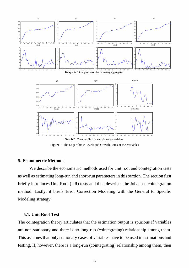
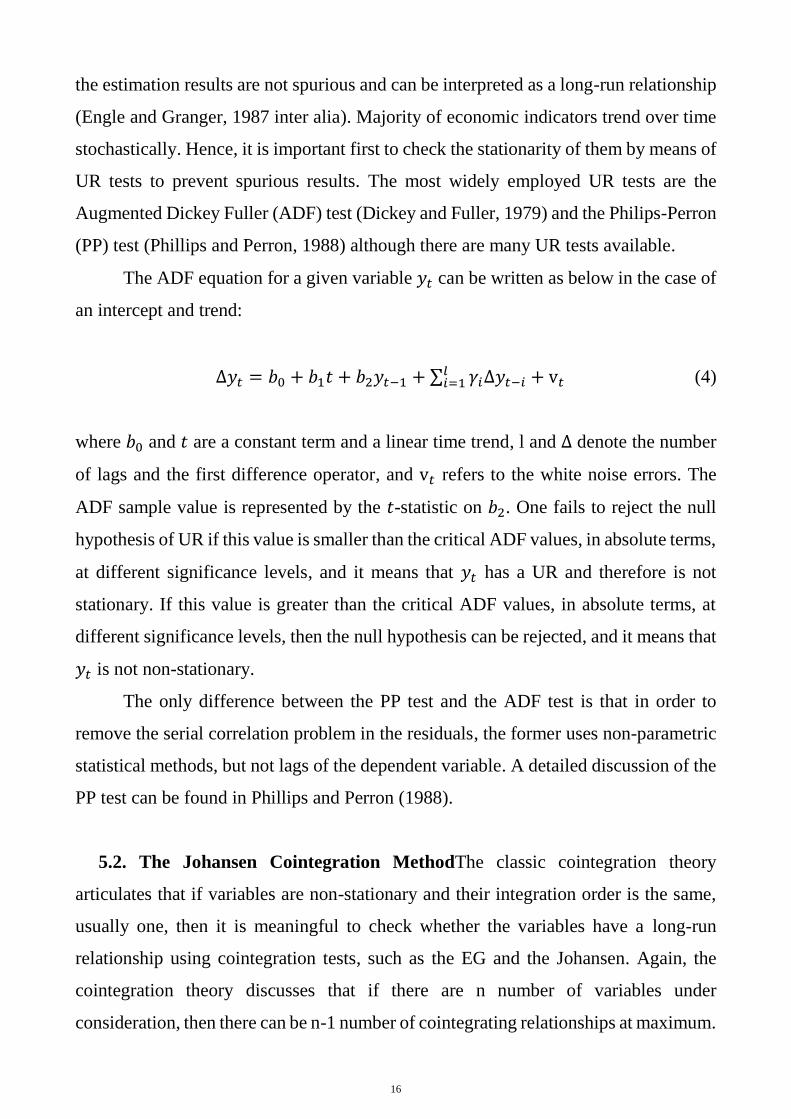
For illustrative purpose, the graphs below portray the logarithmic levels and

growth rates of the variables12.

11 Since government bond rate started in 1994, thereby leaving very small sample for econometric estimations where we use VAR

which is very degree of freedom consuming, we did not consider this interest rate measure. 12 Again, these are level and first difference for RLEND as it is not in logarithmic expression.

15

7

8

9

10

11

12

13

70 75 80 85 90 95 00 05 10 15

m0

7

8

9

10

11

12

13

14

70 75 80 85 90 95 00 05 10 15

m1

8

9

10

11

12

13

14

15

70 75 80 85 90 95 00 05 10 15

m2

8

9

10

11

12

13

14

15

70 75 80 85 90 95 00 05 10 15

m3

-.1

.0

.1

.2

.3

.4

.5

.6

70 75 80 85 90 95 00 05 10 15

d(m0)

-.2

.0

.2

.4

.6

.8

70 75 80 85 90 95 00 05 10 15

d(m1)

-.1

.0

.1

.2

.3

.4

.5

.6

70 75 80 85 90 95 00 05 10 15

d(m2)

.0

.1

.2

.3

.4

.5

.6

70 75 80 85 90 95 00 05 10 15

d(m3)

Graph A. Time profile of the monetary aggregates.

12.8

13.2

13.6

14.0

14.4

14.8

70 75 80 85 90 95 00 05 10 15

gdp

1

2

3

4

5

70 75 80 85 90 95 00 05 10 15

pgdp

0

2

4

6

8

10

70 75 80 85 90 95 00 05 10 15

RLEND

-.3

-.2

-.1

.0

.1

.2

.3

70 75 80 85 90 95 00 05 10 15

d(gdp)

-0.4

0.0

0.4

0.8

1.2

70 75 80 85 90 95 00 05 10 15

d(pgdp)

-3

-2

-1

0

1

2

3

70 75 80 85 90 95 00 05 10 15

d(RLEND)

Graph B. Time profile of the explanatory variables.

Figure 1. The Logarithmic Levels and Growth Rates of the Variables

5. Econometric Methods

We describe the econometric methods used for unit root and cointegration tests

as well as estimating long-run and short-run parameters in this section. The section first

briefly introduces Unit Root (UR) tests and then describes the Johansen cointegration

method. Lastly, it briefs Error Correction Modeling with the General to Specific

Modeling strategy.

5.1. Unit Root Test

The cointegration theory articulates that the estimation output is spurious if variables

are non-stationary and there is no long-run (cointegrating) relationship among them.

This assumes that only stationary cases of variables have to be used in estimations and

testing. If, however, there is a long-run (cointegrating) relationship among them, then

16

the estimation results are not spurious and can be interpreted as a long-run relationship

(Engle and Granger, 1987 inter alia). Majority of economic indicators trend over time

stochastically. Hence, it is important first to check the stationarity of them by means of

UR tests to prevent spurious results. The most widely employed UR tests are the

Augmented Dickey Fuller (ADF) test (Dickey and Fuller, 1979) and the Philips-Perron

(PP) test (Phillips and Perron, 1988) although there are many UR tests available.

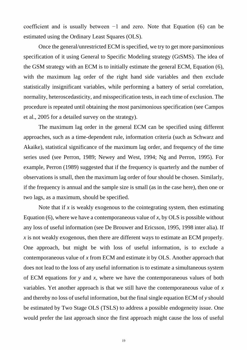
The ADF equation for a given variable 𝑦𝑡 can be written as below in the case of

an intercept and trend:

Δ𝑦𝑡 = 𝑏0 + 𝑏1𝑡 + 𝑏2𝑦𝑡−1 + ∑ 𝛾𝑖Δ𝑦𝑡−𝑖𝑙𝑖=1 + v𝑡 (4)

where 𝑏0 and 𝑡 are a constant term and a linear time trend, l and Δ denote the number

of lags and the first difference operator, and v𝑡 refers to the white noise errors. The

ADF sample value is represented by the 𝑡-statistic on 𝑏2. One fails to reject the null

hypothesis of UR if this value is smaller than the critical ADF values, in absolute terms,

at different significance levels, and it means that 𝑦𝑡 has a UR and therefore is not

stationary. If this value is greater than the critical ADF values, in absolute terms, at

different significance levels, then the null hypothesis can be rejected, and it means that

𝑦𝑡 is not non-stationary.

The only difference between the PP test and the ADF test is that in order to

remove the serial correlation problem in the residuals, the former uses non-parametric

statistical methods, but not lags of the dependent variable. A detailed discussion of the

PP test can be found in Phillips and Perron (1988).

5.2. The Johansen Cointegration MethodThe classic cointegration theory

articulates that if variables are non-stationary and their integration order is the same,

usually one, then it is meaningful to check whether the variables have a long-run

relationship using cointegration tests, such as the EG and the Johansen. Again, the

cointegration theory discusses that if there are n number of variables under

consideration, then there can be n-1 number of cointegrating relationships at maximum.

17

However, only the Johansen test is enable to discover number of cointegrating

relationship among the variables if such relationships is more than one (Engle and

Granger, 1986; Johansen, 1988; Enders, 2010). Once the Johansen test suggests only

one cointegrating relationship among the variables, then other cointegration tests such

as the EG and the ARDLBT can be used or their long- and short-run estimations can

be performed as a robustness check.

The full information maximum likelihood of the Vector Error Correction Model

(VECM) of Johansen (1988) and Johansen and Juselius (1990) can be expressed as

follows:

∆𝑧𝑡 = Π𝑧𝑡−1 + ∑ Γ𝑖∆𝑧𝑡−𝑖𝑘−1𝑖=1 + c + e𝑡 (5)

where, 𝑧𝑡 is a (n × 1) vector of the n endogenous/modeled variables, c is a (n × 1) vector

of constants, Γ represents a (n × (k − 1)) matrix of short-run coefficients, e𝑡 denotes a

(n × 1) vector of white noise residuals, and Π is a (n × n) coefficient matrix. If the

matrix Π has reduced rank (0 < r < n), it can be split into a (n × r) matrix of loading

coefficients α, and a (n × r) matrix of cointegrating vectors β. The former indicates the

importance of the cointegration relationships in the individual equations of the system

and of the speed of adjustment to disequilibrium, while the latter represents the long-

term equilibrium relationship, so that Π = αβ′.

Johansen’s reduced rank regression approach of testing for cointegration

estimates the matrix Π in an unrestricted form first and then tests whether the restriction

implied by the reduced rank of Π can be rejected. In particular, the number of the

independent cointegrating vectors depends on the rank of Π, which in turn is

determined by the number of its characteristic roots that are different from zero. Max-

eigenvalue and Trace test statistics are used to test for nonzero characteristic roots.

Note that significance, stationarity, and weak exogeneity tests are usually

conducted in the Johansen framework, using estimated VECM (Johansen, 1992a, b). If

a given variable in the long-run space is significant, then the null hypothesis of

corresponding β is zero can be rejected. Multivariate stationarity or trend stationarity

of a given variable assumes that (1 0 0)’ restriction on long-run coefficients cannot be

18

rejected. If a given variable is weakly exogenous, it implies that the null hypothesis of

corresponding α is zero cannot be rejected. The weak exogeneity indicates that

deviations from the long-run relationship does not feed back to the variable.

Small Sample Bias Correction in the Johansen Method

Johansen (2002) discussed that in the case of small samples, the Max-eigenvalue or

Trace test statistics are biased to reject the null hypothesis of no cointegration.

Regarding this issue, Reinsel and Ahn (1992) developed a 𝑇−𝑘𝑛

𝑇 correction to the Max-

eigenvalue or Trace test statistics; where k is the lag length of the underlying Vector

Autoregressive (VAR) model in levels and n and T are the number of endogenous

variables and observations, respectively.

5.3. Error Correction Model with the General to Specific Modeling Strategy

This sub-section briefly describes that if the variables are cointegrated, then how short-

run relationships among variables can be estimated using an ECM13.

In the case of single explanatory variable, x, for simplicity, a general or

unrestricted ECM of the dependent variable, y, is as follows:

∆𝑦𝑡 = φ0 + φ𝑦ε̂𝑡−1 + ∑ φ1𝑖∆𝑦𝑡−𝑖𝑝𝑖=1 + ∑ φ2𝑖∆𝑥𝑡−𝑖

𝑝𝑖=0 + 𝑣𝑡 (6)

where 𝑝 indicates the maximum lag order and 𝑣𝑡 is the residuals that are assumed to

be white noise. Engle and Granger (1986) showed that if variables are cointegrated,

then there should be an ECM representation of them which is represented by Error

Correction Term (ECT), ε̂𝑡−1. Furthermore, according to cointegration theory, if there

is a stable cointegration relationship between the variables, then the coefficient on

ECT, i.e., φ𝑦 must be negative and statistically significant (see Engle and Granger,

1986 among others). This coefficient is known as the Speed of Adjustment (SoA)

13 Shortly note that the short-run relationship should be estimated using a VAR or an ARDL of stationary conditions of

the variables, where an error correction term is dropped, if the variables are not cointegrated.

19

coefficient and is usually between −1 and zero. Note that Equation (6) can be

estimated using the Ordinary Least Squares (OLS).

Once the general/unrestricted ECM is specified, we try to get more parsimonious

specification of it using General to Specific Modeling strategy (GtSMS). The idea of

the GSM strategy with an ECM is to initially estimate the general ECM, Equation (6),

with the maximum lag order of the right hand side variables and then exclude

statistically insignificant variables, while performing a battery of serial correlation,

normality, heteroscedasticity, and misspecification tests, in each time of exclusion. The

procedure is repeated until obtaining the most parsimonious specification (see Campos

et al., 2005 for a detailed survey on the strategy).

The maximum lag order in the general ECM can be specified using different

approaches, such as a time-dependent rule, information criteria (such as Schwarz and

Akaike), statistical significance of the maximum lag order, and frequency of the time

series used (see Perron, 1989; Newey and West, 1994; Ng and Perron, 1995). For

example, Perron (1989) suggested that if the frequency is quarterly and the number of

observations is small, then the maximum lag order of four should be chosen. Similarly,

if the frequency is annual and the sample size is small (as in the case here), then one or

two lags, as a maximum, should be specified.

Note that if x is weakly exogenous to the cointegrating system, then estimating

Equation (6), where we have a contemporaneous value of x, by OLS is possible without

any loss of useful information (see De Brouwer and Ericsson, 1995, 1998 inter alia). If

x is not weakly exogenous, then there are different ways to estimate an ECM properly.

One approach, but might be with loss of useful information, is to exclude a

contemporaneous value of x from ECM and estimate it by OLS. Another approach that

does not lead to the loss of any useful information is to estimate a simultaneous system

of ECM equations for y and x, where we have the contemporaneous values of both

variables. Yet another approach is that we still have the contemporaneous value of x

and thereby no loss of useful information, but the final single equation ECM of y should

be estimated by Two Stage OLS (TSLS) to address a possible endogeneity issue. One

would prefer the last approach since the first approach might cause the loss of useful

20

information while the second approach has some system-specific complications in

estimation and disadvantages (e.g. if there is an issue in one equation, it will

contaminate others in the system). Note that it is important first to check whether

contemporaneous value of x in the final ECM specification causes an endogeneity

issue. For this purpose, endogeneity test, e.g. Durbin-Wu-Hausman test, can be applied.

If the test indicates that the contemporaneous value of x is not endogenous, then there

is no gain from the TSLS estimation and it is econometrically proved that the OLS is

the best estimator.

6. Empirical Analysis

Following the conventional sequence of the procedures for cointegration and

error correction analyses, we first perform unit root tests to determine order of

integration of the variables and then check whether or not they are cointegrated. If the

variables are cointegrated, then we estimate parameters of this cointegrated

relationship. As a next step, we estimate error correction representation of this long-

run relationship, using general to specific modeling approach. Finally, we perform a

number of residuals and stability diagnostics tests to make sure that our final ECM

specification has well-behaved residuals and does not suffer from any instability

related to coefficients and/or relationship.

6.1. Unit Root Tests Results

We ran the ADF and PP equations in all the three possible combinations of the

deterministic variables, i.e. intercept and trend, intercept and no trend as well as no

intercept and no trend. Table 3 reports results from those test specifications, in which

the deterministic regressors are included or excluded, conditioned upon their statistical

significance.

21

Table 3: The URT Test Results

Variable The ADF Test The PP Test

Test Value C t None k Test Value C t None

m0 -1.39 x x 0 -1.39 x x

m1 -1.42 x x 0 -1.48 x x

m2 -1.98 x x 0 -1.93 x x

m3 -1.82 x x 0 -1.80 x x

gdp -2.05 x x 0 -2.11 x x

pgdp -0.68 x 0 -0.69 x

RLEND -5.24*** x x 1 -1.52 x x

Δm0 -6.30*** x x 0 -7.53*** x x

Δm1 -3.29*** x 0 -3.34** x

Δm2 -3.31** x 0 -3.24** x

Δm3 -3.18** x 0 -3.30** x

Δgdp -6.90*** x 0 -6.90*** x

Δpgdp -6.49*** x 0 -6.47*** x

ΔRLEND -5.48 *** 1 -2.91*** x Notes. ADF and PP denote the Augmented Dickey-Fuller and Phillips-Perron tests, respectively. Maximum lag order is set to two, and optimal lag

order (k) is selected based on the Schwarz criterion in the tests. ***, **, and * indicate rejection of the null hypotheses of unit root at the 1%, 5%, and 10% significance levels, respectively. The critical values for the tests are taken from MacKinnon (1996). Estimation period: 1987-2016. None

means that neither intercept nor trend is included in test equation. Note again that final UR test equation can include one of the three: intercept (C),

intercept and trend (t), and none of them (None). x indicates that the corresponding option is selected in the final UR test equation.

The PP test sample statistics decisively fail to reject the null hypothesis of unit

root for the log levels of the variables, i.e. monetary aggregates, income, price, and

interest rate. The ADF test statistics also reach up the same conclusion for the variables,

except for RLEND. According to the ADF test, RLEND is trend-stationary since the

sample value of -5.24 is greater than even the critical value at the 1 percent significance

level in absolute term. However, graphical illustration of the variable in Graph B in

Figure 1 strongly rejects trend stationarity of the variable and instead suggests non-

stationarity. Moreover, the PP test also indicates that the variable is a unit root process.

Thus, we conclude that RLEND is non-stationary, i.e. follows unit root process like

other variables above.

The tests statistics profoundly reject the null hypothesis for the first difference

of the log levels of all the variables as indicated in the bottom part of Table 3.

Thus, as a summary of the unit root exercise, we conclude that all the variables

are non-stationary in their log level but stationary in their first difference. In other

words, their integration order is one, i.e. they are I(1) variables.

22

6.2. Cointegration Tests Results

We should conduct the cointegration test to see whether a long-run relationship exists

among the variables as they are all I(1) process. As discussed in the methodological

section, in case of more than two variables, only the Johansen method can properly

reveal out the number of cointegrated relationships. Therefore, we check the existence

of cointegration using the Johansen method as we have four variables in this analysis14.

Following the Johansen method (see Johansen, 1988; Johansen and Juselius, 1990;

Juselius, 2006), we first specify a VAR of the four endogenous variables with the lag

order of two as a maximum as we have a small number of observations15. We also

include intercept and trend in the VAR as exogenous variables. Then we perform the

Lag Exclusion test and Lag Order Selection Criteria to identify optimal lag order. The

former test indicates that two lags cannot be reduced to one lag without loss of

information. Regarding the latter, all the information criteria, i.e. Likelihood Ratio,

Final Prediction Error, Akaike, and Hanna-Quinn, indicate that two lag is optimal while

Schwarz prefers one lag. In order to make proper decision and more robust results, we

estimate both VARs, i.e. one with two lags and another with one lag, and inspect them.

The VAR with two lags has well-behaved residuals in terms of having serial

correlation, normal distribution, and homoscedasticity as well as it is also stable over

time as documented in panels A through D of Table 4. As for the VAR with one lag,

its residuals have first-order autoregressive process which is a serious problem.

Therefore, we opt the VAR with two lags for our further tests and estimations.

To conduct the Johansen cointegration test, we transformed the VAR to VECM.

The test results are reported in panels E and F of Table 4.

14 It is worth noting that we used all the monetary aggregates in turn as a measure of money demand along with income,

price, and interest rate. However, long-run as well as short-run analyses show that M2 aggregate is a more suitable

measure for the Saudi Arabian economy in the given period of time. 15 Estimation sample covers 1989-2016 as our data start in 1987, and we select lag order of two for the VAR.

23

Table 4: The VAR Residual Diagnostics and Cointegration Tests Results

Panel A: Serial Correlation LM Test a Panel E: Johansen Cointegration Test Summary

Lags LM-Statistic P-value Data Trend: None None Linear Linear Quadratic

1 18.64 0.29 Test Type: (a) No C and t (b) Only C (c) Only C (d) C and t (e) C and t

2 21.84 0.15 Trace: 1 2 1 1 1

3 9.77 0.88 Max-Eig: 1 0 0 1 1

Panel B: Normality Test b Panel F: Johansen Cointegration Test Results for type (d)

Statistic χ2 d.f. P-value Null hypothesis: r =0 r ≤ 1

r ≤ 2

r ≤ 3

Skewness 4.53 4 0.34 λtrace 83.72*** 41.06*

16.04

6.62

Kurtosis 3.18 4 0.53 λa trace 59.80* 29.33 11.46 4.73

Jarque-Bera 7.70 8 0.46 λmax 42.66*** 25.02* 9.42 6.62

λa max 30.47* 17.87 6.73 4.73

Panel C: Heteroscedasticity Test c Panel D: VAR Stability Test

White χ2 d.f. P-value No root lies outside the unit circle.

Statistic 204.37 180 0.10

Notes. a The null hypothesis in the Serial Correlation LM Test is that there is no serial correlation at lag order h of the residuals; b System normality test with

the null hypothesis of the residuals are multivariate normal. c White Heteroscedasticity Test takes the null hypothesis of no cross terms heteroscedasticity in the

residuals. χ2is Chi-squared. d.f. means degree of freedom. C and t indicate intercept and trend. r is rank of Π matrix, i.e., number of cointegrated equations. λtrace and λmax

are the Trace and Max-Eigenvalue statistics, while λa trace and λa

max are adjusted version of them. *** and * denote rejection of null hypothesis at

the 1% and 10% significance levels. Critical values for the cointegration test are taken from MacKinnon et al. (1999); Estimation period: 1989-2016.

Although we reportd the test results for all the possible five versions, social and

economic processes are usually better represented by versions (c) and (d) in panel E of

Table 4. Versions (a) and (e) should not be considered because neither m2 has zero

autonomous level nor it has quadratic trend. Version (b) indicates either two or no

cointegrated relationship, both of them are not relevant as usually there is only one

long-run relationship between money and its fundamentals. Moreover, this version

implies that the average growth rate of Δm2 is zero, which is not the case from the

variable’s time profile in Graph A of Figure 1 and its ADF and PP test specification in

Table 3. Thus, we have only versions (c) and (d) to consider. We prefer (d) to (c)

because of the following reasons. First, (d) contains trend in the long-run relation of

the money demand. One should argue economically that time trend captures

innovations and developments in the financial and monetary sectors over time and

hence should be allowed in the long-run space. Additionally, time profile of m2 as well

as the selected ADF and PP unit root test specification for the variable contain time

trend. Furthermore, the trend is statistically significant in the long-run equation as

reported in panel B of Table 5. Moreover, the Trace and the Max-eigenvalue statistics

are consistent each other and indicate one cointegrated relationship. It is also worth

noting that apart from our explanation above, we estimate the long-run equation in all

the versions for robustness check purposes. Only version (d) produces statistically

24

significant coefficients with economically meaningful signs and sizes for the

explanatory variables as well as speed of adjustment16.

Thus, we conclude that long-run equation estimated in version (d) produces

reasonable and consistent results. Hence we will use this specification for further

testing and interpretation purposes.

Both the Trace and Max-Eigenvalue statistics indicate only one cointegrated

relationship after adjusting the statistics for small sample bias in version (d) as

documented in panel D of Table 4.

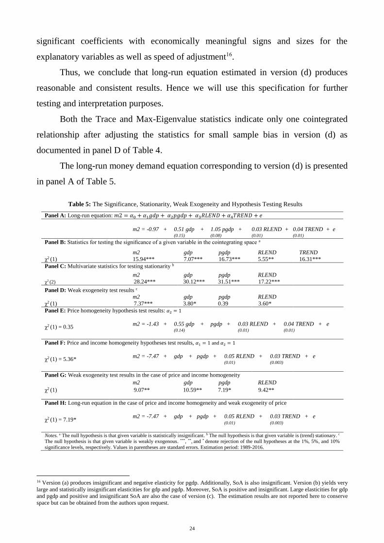
The long-run money demand equation corresponding to version (d) is presented

in panel A of Table 5.

Table 5: The Significance, Stationarity, Weak Exogeneity and Hypothesis Testing Results

Panel A: Long-run equation: 𝑚2 = 𝛼0 + 𝛼1𝑔𝑑𝑝 + 𝛼2𝑝𝑔𝑑𝑝 + 𝛼3𝑅𝐿𝐸𝑁𝐷 + 𝛼4𝑇𝑅𝐸𝑁𝐷 + 𝑒

m2 = -0.97 + 0.51 gdp + 1.05 pgdp + 0.03 RLEND + 0.04 TREND + e (0.15) (0.08) (0.01) (0.01)

Panel B: Statistics for testing the significance of a given variable in the cointegrating space a

m2 gdp pgdp RLEND TREND

χ2 (1) 15.94*** 7.07*** 16.73*** 5.55** 16.31***

Panel C: Multivariate statistics for testing stationarity b

m2 gdp pgdp RLEND

χ2 (2) 28.24*** 30.12*** 31.51*** 17.22***

Panel D: Weak exogeneity test results c

m2 gdp pgdp RLEND

χ2 (1) 7.37*** 3.80* 0.39 3.60*

Panel E: Price homogeneity hypothesis test results: 𝛼2 = 1

χ2 (1) = 0.35 m2 = -1.43 + 0.55 gdp + pgdp + 0.03 RLEND + 0.04 TREND + e (0.14) (0.01) (0.01)

Panel F: Price and income homogeneity hypotheses test results, 𝛼1 = 1 and 𝛼2 = 1

χ2 (1) = 5.36* m2 = -7.47 + gdp + pgdp + 0.05 RLEND + 0.03 TREND + e (0.01) (0.003)

Panel G: Weak exogeneity test results in the case of price and income homogeneity

m2 gdp pgdp RLEND

χ2 (1) 9.07** 10.59** 7.19* 9.42**

Panel H: Long-run equation in the case of price and income homogeneity and weak exogeneity of price

χ2 (1) = 7.19* m2 = -7.47 + gdp + pgdp + 0.05 RLEND + 0.03 TREND + e

(0.01) (0.003)

Notes. a The null hypothesis is that given variable is statistically insignificant. b The null hypothesis is that given variable is (trend) stationary. c The null hypothesis is that given variable is weakly exogenous. ***, **, and * denote rejection of the null hypotheses at the 1%, 5%, and 10%

significance levels, respectively. Values in parentheses are standard errors. Estimation period: 1989-2016.

16 Version (a) produces insignificant and negative elasticity for pgdp. Additionally, SoA is also insignificant. Version (b) yields very

large and statistically insignificant elasticities for gdp and pgdp. Moreover, SoA is positive and insignificant. Large elasticities for gdp

and pgdp and positive and insignificant SoA are also the case of version (c). The estimation results are not reported here to conserve

space but can be obtained from the authors upon request.

25

Panel B shows that all the explanatory variables as well as trend are statistically

significant at the higher level while panel C indicates that the variables are not trend-

stationary. In other words, they are unit root process. The results here from the

multivariate statistics for stationarity confirm those from the ADF and PP, univariate

unit root tests, reported in Table 3. This signifies robustness of our conclusion on the

integration properties of the variables.

The weak exogeneity tests’ results presented in panel D indicate that all the

variables are weakly exogenous except for m2 at the 5 percent or higher significance

level. However, if one goes for the lower significance level, i.e. 10 percent, then gdp

and RLEND are not weakly exogenous.

Testing theoretical assumptions.

The money demand theory articulates that money demanded and price can be in one-

to-one relationship in the long run. In other words, a 1 percent rise in price level should

translate into 1 percent increase in demand for nominal money balance. We tested this

assumption, and the results are documented in panel E of Table 5. Chi-square values

of 0.35 strongly suggest the null hypothesis of the coefficient on price level being unity

cannot be rejected. In the case of price homogeneity hypothesis, the coefficients on

RLEND and TREND have the same values that they have in the unrestricted long-run

equation, while that for gdp is very similar to each other. Additionally, all of the

coefficients keep their sign and statistical significance. It appears that it is very

reasonable to assume price homogeneity.

Then we tested another hypothesis coming from the money demand theory,

stating that it may be possible that money demanded and income are in one-to-one

relationship in the long run. We tested this hypothesis in the case of price homogeneity.

The results reported in panel F of the table show that the assumption/restriction can be

rejected at the 5 percent level but accepted at the 10 percent significance level. Given

that we have a small number of observation points, one should go for 10 percent

significance level. We did the same and accepted the restriction as a research decision.

Another reason that led us to accept the assumption is that the values of the coefficients

26

on RLEND and TREND are still similar to what they were in the un-restricted case. We

would prefer this specification of the long-run equation, where we have homogeneity

hypothesis for price and income incorporated.

We tested weak exogeneity of the variables for this specification. It appears that

only price is weakly exogenous to the system at the 10 percent significance level as

shown in panel G of the table. Finally, we reached the long-run money demand

specification, where we have price and income homogeneity and weak exogeneity of the

price. The results presented in panel H of Table 5 show that the restrictions are acceptable

at the 10 percent, and RLEND and TREND have statistically significant coefficients with

the same magnitudes as they had before. Although it is at the 10 percent significance

level, because of the above given explanations, we would accept it as a research decision.

Thus, we will calculate the residuals from the long-run specification given in

panel H for our ECM estimation.

6.3. Short-run Analysis

Following the methodological discussion above, we specify our general ECM for 𝛥m2

with the maximum lag order of one since this lag length is satisfactory to remove serial

correlation from the residuals17. Recall that one lag was also optimal in the VECM

estimation above and provided serially uncorrelated residuals. Then we try to get more

parsimonious ECM specification by following GSM strategy. Our final ECM

specification contains the contemporaneous values of 𝛥gdp and 𝛥pgdp along with ECT

term and intercept. Recall that the weak exogeneity test results presented in panel G of

Table 5 show that 𝛥gdp and 𝛥pgdp are not weakly exogenous to the long-run

relationship. Therefore, we estimate the final ECM specification with TSLS as well and

run the Durbin-Wu-Hausman test to see whether 𝛥gdp and 𝛥pgdp are still endogenous.

Difference in J-statistic with the null hypothesis of the variables are exogenous, given

the sample value of 2.52 with the p-value of 0.2818. Thus, we conclude that the variables

17 We also estimated our general ECM with the maximum lag order of two. However, this general ECM yields exactly the same final

specification in terms of number of regressors (and also almost exactly the same signs, sizes, significance of the coefficients, etc.) as the

general ECM with one lag does. However, in the case of general ECM with two lags, we are forced to start estimation from 1990 while it

is 1989 for the general ECM with one lag. Therefore, we preferred the general ECM with one lag as it has one more observation point. 18 We also ran the test for each variable separately, and the test statistics again failed to reject the null hypothesis of exogeneity.

27

are exogenous. Hence there is no endogeneity issue, and the OLS is a better estimator

than the TSLS.

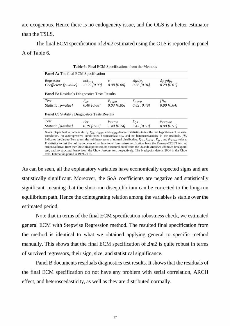
The final ECM specification of 𝛥m2 estimated using the OLS is reported in panel

A of Table 6.

Table 6: Final ECM Specifications from the Methods

Panel A: The final ECM Specification

Regressor 𝑒𝑐𝑡𝑡−1 𝑐 𝛥𝑔𝑑𝑝𝑡 𝛥𝑝𝑔𝑑𝑝𝑡 Coefficient [p-value] -0.29 [0.00] 0.08 [0.00] 0.36 [0.04] 0.29 [0.01]

Panel B: Residuals Diagnostics Tests Results

Test 𝐹𝐴𝑅 𝐹𝐴𝑅𝐶𝐻 𝐹𝐻𝐸𝑇𝑅 𝐽𝐵𝑁

Statistic [p-value] 0.40 [0.68] 0.03 [0.85] 0.82 [0.49] 0.90 [0.64]

Panel C: Stability Diagnostics Tests Results

Test 𝐹𝐹𝐹 𝐹𝐶𝐻𝑂𝑊 𝐹𝑄𝐴 𝐹𝐶𝐻𝑂𝑊𝐹

Statistic [p-value] 0.19 [0.67] 1.49 [0.24] 3.47 [0.53] 0.99 [0.51]

Notes. Dependent variable is 𝛥𝑚2𝑡. 𝐹𝐴𝑅, 𝐹𝐴𝑅𝐶𝐻, and 𝐹𝐻𝐸𝑇𝑅 denote F statistics to test the null hypotheses of no serial

correlation, no autoregressive conditioned heteroscedasticity, and no heteroscedasticity in the residuals. 𝐽𝐵𝑁

indicates the Jarque-Bera to test the null hypotheses of normal distribution. 𝐹𝐹𝐹 , 𝐹𝐶𝐻𝑂𝑊 , 𝐹𝑄𝐴 , and 𝐹𝐶𝐻𝑂𝑊𝐹 refer to

F statistics to test the null hypotheses of no functional form miss-specification from the Ramsey-RESET test, no structural break from the Chow breakpoint test, no structural break from the Quandt-Andrews unknown breakpoint

test, and no structural break from the Chow forecast test, respectively. The breakpoint date is 2004 in the Chow

tests. Estimation period is 1989-2016.

As can be seen, all the explanatory variables have economically expected signs and are

statistically significant. Moreover, the SoA coefficients are negative and statistically

significant, meaning that the short-run disequilibrium can be corrected to the long-run

equilibrium path. Hence the cointegrating relation among the variables is stable over the

estimated period.

Note that in terms of the final ECM specification robustness check, we estimated

general ECM with Stepwise Regression method. The resulted final specification from

the method is identical to what we obtained applying general to specific method

manually. This shows that the final ECM specification of 𝛥m2 is quite robust in terms

of survived regressors, their sign, size, and statistical significance.

Panel B documents residuals diagnostics test results. It shows that the residuals of

the final ECM specification do not have any problem with serial correlation, ARCH

effect, and heteroscedasticity, as well as they are distributed normally.

28

Stability of the Money Demand Relationship

Finally, we performed different tests to check stability of the final ECM specification of

money demand. We first ran residuals and coefficient recursive estimation tests. The

results are illustrated in Figure 2.

-.15

-.10

-.05

.00

.05

.10

.15

94 96 98 00 02 04 06 08 10 12 14 16

Recursive Residuals ± 2 S.E.

-0.4

-0.2

0.0

0.2

0.4

0.6

0.8

1.0

1.2

1.4

94 96 98 00 02 04 06 08 10 12 14 16

CUSUM of Squares 5% Significance Graph A. Recursive residuals Graph B. CUSUM of Squares test

0

-.15

-.10

-.05

.00

.05

.10

.15

94 96 98 00 02 04 06 08 10 12 14 16

N-Step Probability

Recursive Residuals

-0.4

-0.2

0.0

0.2

0.4

0.6

0.8

1.0

94 96 98 00 02 04 06 08 10 12 14 16

Recursive C(1) Estimates

± 2 S.E.

-6

-4

-2

0

2

4

94 96 98 00 02 04 06 08 10 12 14 16

Recursive C(2) Estimates

± 2 S.E.

-4

-3

-2

-1

0

1

2

3

94 96 98 00 02 04 06 08 10 12 14 16

Recursive C(3) Estimates

± 2 S.E.

-4

-2

0

2

4

6

8

94 96 98 00 02 04 06 08 10 12 14 16

Recursive C(4) Estimates

± 2 S.E. Graph C. N-step Forecast test Graph D. Recursive Coefficients

Figure 2: Recursive Estimation Tests Results for the Final ECM.

The first three recursive residuals test results demonstrate that the residuals are quite

well-behaved over time, except a spike in 2004. The last graph illustrates that all the

estimated four coefficients of the final ECM specification are very stable over time. The

coefficients as well as residuals stability are very important in using the model for policy

analysis and forecasting purposes. Since the recursive coefficient estimate shows that

the coefficients are time invariant and the Ramsey-Reset misspecification test indicates

that the final ECM specification does not have any functional form problem, we are only

concerned about the spike occurred in 2004 in the residuals. To further address this issue,

we ran different breakpoint tests to investigate whether the spike in 2004 causes a

structural break. Panel C of Table 6 presents the tests’ results.

We ran Chow breakpoint test and Chow forecast tests to check whether there is a

breakpoint in 2004. Both tests’ results failed to reject the null hypothesis of no breakpoint

29

as panel C documents that estimated sample F-statistics of 1.49 and 0.99 respectively

are quite smaller than the critical F-values. As a further robustness, we also ran the

Quandt-Andrews unknown breakpoint test and let the test determine endogenously if

there is a break. The obtained sample value of the Average Wald F-statistic of 3.47 with

the quite high p-value indicate that there is no break in the money demand relationship.

The rest five statistics of the Quandt-Andrews test, such as the Average and Maximum

Likelihood Ratio F-statistics and Maximum Wald F-statistic, also show that no break

occur in the relationship. Thus, we conclude that the spike in 2004 does not cause any

structural change either in the estimated parameters or in the relationship between money

demand and its drivers.

7. Discussion of the Empirical Results

The Unit Root tests’ results show the natural logarithmic expressions of the

monetary aggregates, GDP, GDP Deflator, and RLEND are non-stationary in levels

and stationary in their first difference. In other words, they are all I(1) processes. The

non-stationarity of the variables means that they do not return to their previous mean,

and the mean value changes from one time period to another as they are trending over

time. There are two main implications, among others, for the non-stationarity of the

variables. The future values of the variables form randomly and thus it is difficult to

forecast them accurately. If there is a shock affecting the variables, it might have a

permanent effect on their time profile. Inversely, stationarity of the variables, in our

case the first difference of them, implies that they are mean reverting in the sense that

past, present, and future mean values will be very close to each other19. Hence, it is

easier to predict future trajectory of the variables when they are in stationary form.

These features should be taken into consideration especially when undertaken research

does forecasting exercise.

The Johnsen cointegration tests conclude that there is a cointegrated relationship

among the M2 monetary aggregate, GDP, GDP Deflator, and RLEND. It means that

19 Theoretical definition of the stationarity assumes that mean, variance, and covariance values of given variables do not change over

time. It is called strict stationarity, which is not the case for the socio-economic variables. Therefore, stationarity in economics is

characterized as weak stationarity (Enders, 2010; Guajarati and Porter, 2009).

30

the variables move together over time. To put it differently, there is a common/shared

trend among them. This implies that the relationship between the levels of the variables

is not spurious, meaning that the estimated coefficients from the level relationship are

valid for analysis and forecasting. In this regard, estimated unrestricted long-run

equation of the money demand, reported in panel A of Table 6, indicates that ceteris

paribus, a 1 percent increase in GDP, PGDP, and RLEND, leads to 0.51 percent, 1.05

percent, and 3 percent (0.03*100) increase in the demand for M2 monetary aggregate

in the long-run. The equation also shows that the factors changing over time, which are

not included in the equation, caused 4 percent increase in the M2 demand each year

over the period 1989-2016. After testing the theoretical predictions, we conclude that

M2 can be in one-to-one relationship with PGDP and GDP in the long -run in panel F.

It means that a 1 percent increase in price and income is associated with 1 percent

increase in demand for broad money.

What follows is the explanation of the impact of the explanatory variables on

M2. Note that we have a brief explanation here as our results are consistent with money

demand theory as well as being in line with the empirical studies on money demand.

Again, as theoretically expected, income has statistically significant and positive

impact on the money demand. It can be interpreted as a transaction motive for money

works in the Saudi economy, meaning that when economic agents have more income,

then they will need more money to spend on goods and services. Our finding is in line

with the findings of other money demand studies for the Saudi economy, such as

Bahmani (2008) and Banafea (2012). Additionally, the empirical analysis shows that

this transaction motive has one-to-one relationship with M2 in the long -run.

The positive effect of price level on money demand can be explained in a way

that when price level is higher in the Saudi economy, then goods and services will be

more expensive to purchase than they were before. This finding of our research is also

in line with the earlier money demand studies on the Saudi Arabia.

We found that demand for M2 monetary aggregate is positively influenced by

the 3-month SAIBOR rate. Whether interest rate has negative (or positive) impact on

money demand depends on both the interest rate and money demand considered in the

31

empirical analysis. For example, there should be a negative relationship if one

considers demand deposit rate and M0, i.e. cash in circulation, measures of interest rate

and money, respectively, simply because an increase in return on demand deposit will

induce economic agents to put their cash in demand deposits. However, if one

considers demand deposit rate and M1 that is narrow money aggregate, which is sum

of cash in circulation and demand deposits, then the relationship should be positive.

The reason is that raising the interest rate will increase demand deposits, which is a

part of M1. In this regard, we would explain the positive relationship found in our

analysis as follows. When loan rate is high, then deposit rate will be high too as these

two are closely linked to each other. For instance, if loan rate is high, then commercial

banks will increase deposit rate to attract more money from the economic agents and

thereby offer more loans. Higher deposit rate will induce economic agents to put more

money in their deposit accounts. In order to do so, they will be interested in converting

their other assets, such as real state, land area, and jewelry, into money and putting it

in their deposit accounts, which will result in an increase in M2 monetary aggregate.

Finally, we found a positive effect of time trend on M2. The time trend can be

considered a storage of factors that changes over time, such as institutional and

technological developments, innovations, and others in the economy, especially in the

money market.

Regarding the short-run relationship, the obtained final ECM specification

reported in panel A of Table 6 shows that only ECT, the growth rates of GDP, and

PGDP have statistically significant impact on the growth rate of demand for M2.

Statistically significant SoA on ECT is theoretically expected as it has a negative sign.

Interpretation of it is that any shocks causing the relationship, between the money and

its fundamentals, to deviate from the long-run equilibrium path will be corrected back

to this equilibrium. The size of SoA indicates that 29 percent of the deviation will be

corrected back to the equilibrium level within one year, meaning that the complete

correction will take slightly more than three years. All this shows that long-run

relationship between M2 and its determinants is stable, and any shocks to this

relationship will be temporary in the Saudi economy.

32

The final ECM further shows that contemporaneous values of income and price

are positively related to M2 growth rate. Precisely speaking, a 1 percentage point

increase in GDP and PGDP will result in 0.36 and 0.29 percentage points increase in

demand for M2 respectively. It is theoretically and empirically expected as we

explained for the long-run results above. It is worth noting that short-run effects of the

income and price appear smaller than those in the long -run.

Finally, we conduct a battery of different stability tests, as a robustness check,

to see whether there is any break in money demand relationship in Saudi Arabia. The

general conclusion from these tests, documented in panel C and Figure 2, is that the

relationship between M2 and its drivers, such as income, price, and interest rate, is

stable over the period considered.

8. Conclusion

For policymakers, it is important to understand how money demand behaves in

order to design the suitable monetary and fiscal policies. Consequently, there has been

continuous effort from researchers in academia and analysts from government and

private entities, aiming to comprehend the influential elements that could explain the

variation in money demand. Observing the current literature on money demand

indicates that there are an inadequate number of studies estimating the demand for

money in Saudi Arabia. This in turn has encouraged us to fill out the gap in the

literature by employing the most recent data, up to 2016, as well as relying on advanced

econometric procedures to opt the most appropriate form of money demand function.

In specific, in this paper, we attempted to examine long-run relationship between

money demand and its determinants as well as short-run dynamics among them in the

Saudi economy. We employed the Johansen cointegration test with small sample bias

correction in order to properly address the existence of long-run relationship between

demand for money and its fundamentals. The result indicates that there is a long-run

relationship among broad money, income, price, and interest rate. We also tested the

theoretical predictions and revealed out that both income and price homogeneity

hypotheses hold for the Saudi money demand function. In the short-run analysis, we

33

applied the GtSMS to our ECM estimation to properly specify set of explanatory

variables and found that growth rate of money demand is associated with error

correction term as well as growth rates of income and price. Additionally, it is found

that long-run relationship is stable over time as short-run deviations can be adjusted

towards the long-run equilibrium level. Finally, we applied different structural break

tests to our final ECM as it is important to know whether a given money demand

relationship is stable over time. The tests show that the estimated money demand

relationship is stable over time.

Lastly, being able to understand how money demand in Saudi Arabia behaves

over both short and long runs is essential for policymakers. In particular, maintaining

a stable money demand function is a key requirement to forecast the nominal exchange

rate based on the monetary model of exchange rate. Likewise, observing money

demand fluctuations enables monetary authorities to watch the liquidity level. By doing

so, monetary authorities may need to use their available policy instruments to sustain

stable liquidity levels.

Acknowledgments

The views expressed in this study are those of the authors and do not necessarily

represent the views of their affiliated institutions. The authors are responsible for all

errors and omissions.

34

Reference

Abdulkheir, A. Y. (2013). An analytical study of the demand for money in Saudi Arabia.

International Journal of Economics and Finance, 5 (4), 31 – 38.

Al-Bassam, K.A. (1990). Money demand and supply in Saudi Arabia: An empirical

analysis (PhD Thesis, University of Leicester).

Al-Jasser, M., & Banafe, A. (2005). Monetary policy transmission mechanism in Saudi

Arabia. BIS Papers No. 35, 439- 442.

AlKaswani, M., & Al-Towaijari, H. (1999). Cointegration, error correction, and the

demand for money in Saudi Arabia. Economia Internazionale/ International

Economics, 52 (3), 299-308.

Al Rasasi, M. (2016). On the stability of money demand in Saudi Arabia. Saudi Arabian

Monetary Agency Working Paper, WP/16/6.

Alsamara, M., Mrabet, Z., Dombrecht, M., & Barkat, K. (2017). Asymmetric responses

of money demand to oil price shocks in Saudi Arabia: A non-linear ARDL

approach. Applied Economics, 49 (37), 3758-3769.

Andrews, D.W.K. (1993). Tests for parameter instability and structural-change with

unknown change point. Econometrica, 61 (4), 821-856.

Andrews, D.W.K., & Ploberger, W. (1994). Optimal tests when a nuisance parameter is

present only under the alternative. Econometrica, 62 (6), 531-549.

Arrau, P., & De Gregorio, J. (1993). Financial innovation and money demand: Application

to Chile and Mexico. Review of Economics & Statistics, 75 (3), 524-530.

Bahmani, S. (2008). Stability of the demand for money in the Middle East. Emerging

Markets Finance & Trade, 44 (1), 62 – 83.

Bahmani-Oskooee, M. (2001). How stable is M2 money demand function in Japan? Japan

and the World Economy, 13 (4), 455-461.

Bahmani-Oskooee, M., & Barry, M.P. (2000). Stability of the demand for money in an

unstable country: Russia. Journal of Post Keynesian Economics, 22 (4), 619-629.

Bahmani-Oskooee, M., & Gelan, A. (2009). How stable is the demand for money in

African countries? Journal of Economic Studies, 36 (3), 779-792.

Bahmani-Oskooee, M., & Rahman, H. (2005). Stability of the money demand function in

Asian developing countries. Applied Economics, 37 (7), 216-235.

35

Banafea, W.A. (2012). Essays on structural breaks and stability of the money demand

function (PhD Thesis, Kansas State University).

Banafea, W. A. (2014). Endogenous structural breaks and stability of the money demand

function in Saudi Arabia. International Journal of Economics and Finance, 6 (1),

155 – 164.

Basher, S.A., & Fachin, S. (2014). Investigating long-run demand for broad money in the

Gulf Arab countries. Middle East Development Journal, 6 (2), 199-214.

Breitung, J. (2000). The local power of some unit root tests for panel data. In B. Baltagi,

(Ed.), Advances in Econometrics: Vol. 15. Nonstationary panels, panel

cointegration, and dynamic panels (pp. 161-178). Amsterdam: JAY Press.

Campos, J., Ericsson, N.R., & Hendry, D.F. (2005). General-to-specific modeling: An

overview and selected bibliography. Board of Governors of the Federal Reserve

System. International Finance Discussion Papers, 838. Retrieved from

http://www.federalreserve.gov/pubs/ifdp/2005/838/ifdp838.pdf (accessed on 25

September 2016).

Chow, G.C. (1960). Tests of equality between sets of coefficients in two linear regressions.

Econometrica, 28 (3), 591-605.

Coenen, G., & Vega, J-L. (2001). The demand for M3 in the Euro Area. Journal of Applied

Econometrics, 16 (6), 727-748.

De Brouwer, G., & Ericsson, N. (1995). Modeling inflation in Australia (Research

Discussion Paper 9510, International Finance Discussion Paper 530). Sydney,

Australia: Reserve Bank of Australia.

De Brouwer, G., & Ericsson, N. (1998). Modeling inflation in Australia. Journal of

Business & Economic Statistics, 16 (4), 433–449.

Di Iorio, F., & Fachin, S. (2014). Saving and investments in the OECD: A panel

cointegration study with a new bootstrap test. Empirical Economics, 46 (4), 1271-

1300.

Dickey, D., & Fuller, W. (1979). Distribution of the estimators for autoregressive time

series with a unit root. Journal of the American Statistical Association, 74 (366),

427–431.

Elliot, G., Rothenberg, T.J., & Stock, J.H. (1996). Efficient tests for an autoregressive unit

root. Econometrica, 64 (4), 813-836.

Enders, W. (2010). Applied econometrics time series (Wiley Series in Probability and

Statistics). Tuscaloosa, AL: University of Alabama.

36

Engle, R.F., & Granger, C.W.J. (1987). Co-integration and error correction:

Representation, estimation, and testing. Econometrica, 55 (2), 251-276.

Gregory, A., & Hansen, B. (1996). Residual-based tests for cointegration in models with

regime shifts. Journal of Econometrics, 70(1), 99–126.

Gujarati, D.N., & Porter, D.C. (2009). Basic econometrics (5th Edition). New York:

McGraw Hill Inc.

Hamdi, H., Said, A., & Sbia, R. (2015). Empirical evidence on the long-run money

demand function in the Gulf Cooperation Council countries. International Journal

of Economics and Financial Issues, 5 (2), 603 – 612.

Hansen, B. (1992). Tests for parameter instability in regressions with I(1) processes.

Journal of Business and Economic Statistics, 10 (3), 321-335.

Harb, N. (2004). Money demand function: A heterogeneous panel application. Applied

Economics Letters, 11 (9), 551 – 555.

Haug, A., & Tam, J. (2007). A closer look at the long-run U.S. money demand: Linear or

nonlinear error correction with M0, M1, or M2? Economic Inquiry, 45 (2), 363-367.

Hondroyiannis, G., Swamy, P.A.V.B., & Tavlas, G.S. (2001). Modelling the long-run

demand for money in the United Kingdom: A random coefficient analysis.

Economic Modelling, 18 (1), 475-501.

Im, K., Pesaran, H., & Shin, Y. (2003). Testing for unit roots in heterogeneous panels.

Journal of Econometrics, 115 (1), 53-74.

Jiang, J. (2016). Modeling money demand in China: Evidence from cointegration analysis.

China Economic Policy Review, 5 (1), 1-8.

Johansen, S. (1988). Statistical analysis of cointegration vectors. Journal of Economic

Dynamics and Control, 12 (2-3), 231-254.

Johansen, S. (1992a). Testing weak exogeneity and the order of cointegration in UK

money demand data. Journal Policy Model, 14 (3), 313–334.

Johansen, S. (1992b). Cointegration in partial systems and the efficiency of single-

equation analysis. Journal of Econometrics, 52 (3), 389–402.

Johansen, S. (2002). A small sample correction for the test of cointegrating rank in the

vector autoregressive model. Econometrica, 70 (5), 1929–1961.

Johansen, S., & Juselius, K. (1990). Maximum likelihood estimated and inference on

cointegration with application to the demand for money. Oxford Bulletin of

Economics and Statistics, 52 (2), 169-210.

37

Juselius, K. (2006). The cointegrated VAR model: Methodology and applications.

Oxford: Oxford University Press.

Kao, C., & Chiang, M. H. (2000). On the estimation and inference of a cointegrated

regression in panel data. In B. Baltagi, (Ed.), Advances in Econometrics: Vol. 15.

Nonstationary panels, panel cointegration, and dynamic panels (161-178).

Amsterdam: JAY Press.

Kia, A. (2006). Economic policies and demand for money: Evidence from Canada.

Applied Economics, 38 (12), 1389-1407.

Kwiatkowski, D., Phillips, P.C.B., Schmidt, P., & Shin, Y. (1992). Testing the null

hypothesis of stationarity against the alternative of a unit root. Journal of

Econometrics, 54 (1-3), 159-178.

Larson, R., Lyhagen, J., & Lothgren, M. (2001). Likelihood-based cointegration tests in

heterogenous panels. Econometrics Journal, 4 (1), 109-142.

Lee, C., Chang, C., & Chen, P. (2008). Money demand function versus monetary

integration: Revisiting panel cointegration among GCC countries. Mathematics and

Computers in Simulation, 79(1), 85-93.

Levin, A., Lin, C., & Chu, C. J. (2002). Unit root tests in panel data: Asymptotic and finite-

sample properties. Journal of Econometrics, 108(1), 1-24.

MacKinnon J. (1996). Numerical distribution functions for unit root and cointegration

tests. Journal of Applied Econometrics, 11 (6), 601–618.

MacKinnon J.G., Alfred A.H., & Leo M. (1999). Numerical distribution functions of

likelihood ratio tests for cointegration. Journal of Applied Econometrics, 14 (5),

563–577.

Maddala, G. S., & Wu, S. (1999). A comparative study of unit root tests with panel data

and a new simple test. Oxford Bulletin of Economics and Statistics, 61(S1), 631–

652.

Masih, M., & Algahtani, I. (2008). Estimation of long-run demand for money: An

application of long-run structural modeling to Saudi Arabia. Economia

Internazionale/ International Economics, 61 (1), 81–99.

Newey, W., & West, K.D. (1992). Automatic lag selection in covariance matrix

estimation. Wisconsin Madison - Social Systems, working paper, Vol. 61.

Ng, S., & Perron, P. (1995). Unit root tests in ARMA models with data-dependent

methods for the selection of the truncation lag. Journal of the American Statistical

Association, 90 (429), 268-281.

38

Nielsen, H.B. (2007). UK money demand 1873-2001: A long-run time series analysis and

event study. Cliometrica, 1 (1), 45-61.

Özdemir, K.A., & Saygılı, M. (2013). Economic uncertainty and money demand stability

in Turkey. Journal of Economic Studies, 40 (3), 314-333.

Pedroni, P. (2001). Fully modified OLS for heterogeneous cointegrated panels. In B.

Baltagi, T. Fomby, & R. Carter Hill (Eds.), Advances in Econometrics: Vol. 15.

Nonstationary panels, panel cointegration, and dynamic panels (pp.93 - 130).

Emerald Group Publishing Limited.

Pedroni, P. (2004). Panel cointegration: Asymptotic and finite sample properties of pooled

time series tests with an application to the PPP hypothesis. Economic Theory, 20

(3), 597-625.

Perron, P. (1989). The great crash, the oil price shock, and the unit root hypothesis.

Econometrica, 57 (6), 1361–1401.

Pesaran, M.H., & Shin, Y. (2002). Long-run structural modelling. Econometric Review,

21 (1), 49-87.

Pesaran, M.H., Shin, Y., & Smith, R.P. (2001). Bounds testing approaches to the analysis

of level relationships. Journal of Applied Econometrics, 16 (3), 289-326.

Phillips, P. (1992). Hyper-consistent estimation of a unit root in time series regression.

Cowles Foundation Discussion Paper, No. 1040.

Phillips, P.C.B, & Hansen, B.E. (1990). Statistical inference in instrumental variables

regression with i(1) processes. Review of Economics Studies, 57 (1), 99-125.

Phillips, P.C.B., & Perron, P. (1988). Testing for unit roots in time series regression.

Biometrika, 75 (2), 335-346.

Rao, B.B., & Singh, R. (2006). Demand for money in India: 1953-2003. Applied

Economics, 38 (11), 1319-1326.

Reinsel, G.C., & Ahn, S.K. (1992). Vector autoregressive models with unit roots and

reduced rank structure: Estimation, likelihood ratio test, and forecasting. Journal of

Time Series Analysis, 13 (4), 353–375.

Said, S.E., & Dickey, D.A. (1984). Testing for unit roots in autoregressive-moving

average models of unknown order. Biometrika, 71(3), 599-607.

Singh, P., & Pandey, M.K. (2012). Is long-run demand for money stable in India? An

application of the Gregory-Hansen model. The IUP Journal of Applied Economics,

XI (2), 59-69.

39

Tümtürk, O. (2017). Stability of money demand function in Turkey. Business and

Economics Research Journal, 8 (1), 35-48.

Wang, Y. (2011). The stability of long-run money demand in the United States: A new

approach. Economics Letters, 111 (1), 60-63.

Zivot, E., & Andrews, D. (1992). Further evidence on the great crash, the oil–price shock,

and the unit root hypothesis. Journal of Business & Economics, 10 (3), 251–270.

Zuo, H., & Park, S.Y. (2011). Money demand in China and time-varying cointegration.

China Economic Review, 22 (3), 330-343.