My goal from the very inception of this project, as reflected in the book’s title, has been to teach researchers how to conduct both mediation and moderation analyses, with an emphasis on the “how to.” I have tried to emphasize hands-on procedures for performing these analyses so that someone reading this book can quickly and readily acquire the set of skills necessary for these analyses. I hope that students who are learning the essentials of statistical analyses will be able to learn from this book what mediation and moderation can do and to more quickly integrate these approaches into their theory, research, and writings.
As I say later in the book, I am convinced that the best learning in statistics occurs through the hands-on experience of setting up a dataset, doing computations, reading the statistical output, graphing the results, and interpreting the resulting patterns. We learn by doing. So I want you, dear reader, to learn these techniques by conducting analyses on sample datasets that I have provided while you are reading this book. In addition, I have provided extra exercises and problems at the end of the substantive chapters so that you can practice these techniques and expand your expertise. (Suggested answers to exercises appear at the end of the book.) Appendix A relates SPSS, Amos, and Mplus syntax for conducting the key types of analyses, and Appendix B contains URLs for useful online material and applets to run related analyses. I have a very pragmatic, practical streak in my personality; I learned from an early age, growing up on a dairy farm in the Midwestern United States, that theory is nice and all, but it is not worth much if it cannot be applied.
I have written this book to encompass both mediation and moderation, harking back to Baron and Kenny’s (1986) seminal article that alerted many of us to the benefit of jointly considering these two statistical techniques.
It is true that both methods describe interesting relationships among three variables (in the simpler versions of both), so it is natural to discuss them together; but it is also true that they sit next to each other uneasily, like teenage boys and girls at a school-sponsored dance. It is not clear how they are similar and different, and although I have taken some pains to explicate this enduring issue in this book, I remain unconvinced that we have utterly resolved the tension between these two techniques. Still, I believe that understanding one assists in the understanding of the other, and this is particularly germane once we begin to learn about and use combinations such as moderated mediation and mediated moderation.
The last issue that I would like to raise concerns the level of this book. For whom is this book written? I believe that higher-level undergraduates and graduate students will benefit chiefly from Chapters 2 (Historical Background), 3 (Basic Mediation), and 5 (Basic Moderation). The other chapters— Chapters 4 (Special Topics in Mediation), 6 (Special Topics in Moderation), and 7 (Mediated Moderation and Moderated Mediation)—will prove more difficult for these readers because they are written with the assumption that the reader knows structural equation modeling and multilevel modeling. Established researchers who know the basics of mediation and moderation and want to be stimulated to learn cutting-edge variations in these techniques (e.g., latent variable moderation) may wish to skim or skip the basic chapters and focus on the three higher-level chapters. I believe that a single book can encompass both entry-level instruction in mediation and moderation and instruction in advanced techniques, and that book is now in your hands. However, I do not believe that all readers will read and benefit from everything in this book; some will read only the basic material and some will read only the advanced material. I want the book to be used in statistics classes, and I also want it to function as a reference book to be taken down and perused from time to time to refresh one’s memory as to how to do a particular analysis. These are my hopes for this progeny of mine that I am launching into the world, and whether it fulfills all of these goals remains to be seen. I realize that certain errors may remain in the book (even after careful vetting from multiple readers), so I would appreciate feedback from readers concerning these issues. If this book serves a useful function, I will be keen to revise, improve, and polish the book for another edition in a few years (after I recover from the exhaustion caused by this one). Finally, I hope that you benefit from reading this book, and enjoy learning about these techniques.
This chapter describes the basic procedures for conducting mediation with multiple regression. This approach is based on the Baron and Kenny (1986) recommendations, and it is the conventional technique that most researchers use today. The sections are as follows:
1. Review of basic rules for mediation
2. How to do basic mediation
3. An example of mediation with experimental data
4. An example of null mediation
5. Sobel’s z versus reduction of the basic relationship
6. Suppressor variables in mediation
7. Investigating mediation when one has a nonsignificant correlation
8. Understanding the mathematical “fine print”: Variances and covariances
9. Discussion of partial and semipartial correlations
10. Statistical assumptions
The reader who perseveres through all of this material will achieve one of the chief goals of the present book, namely, to learn how to perform a mediational analysis with multiple regression. This method is referred to as “basic mediation” because it is the simplest form of mediation that one can perform. Further, if you read all of the auxiliary material that follows (points 6, 7, and 8 in the preceding list), you will understand at a deeper level the mathematical underpinnings of this analytical technique. I suppose that this order of topics to some extent gives you “the dessert before the vegetables,” but I present the material this way to give you a chance to enjoy the thrill of conducting mediation before
moving on to the more mundane issues of understanding the statistical details. In my experience, students are more interested in the latter details if they can actually perform the mediation analysis. And I would strongly encourage you to “eat your vegetables” and learn or review the statistical foundation for this technique.
REVIEW Of BASIC RULES fOR MEdIATION
This chapter is devoted to describing in great detail how to perform a basic mediational analysis. I begin with a straightforward example, progress through several other instances of mediation, show how to make an interpretation of a mediation result, discuss problems and pitfalls with conducting mediational analyses, and conclude by describing the statistical assumptions that must be satisfied in order to perform a valid mediational analysis.
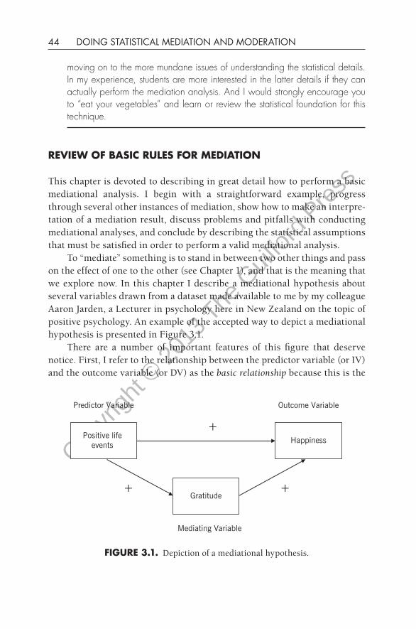
To “mediate” something is to stand in between two other things and pass on the effect of one to the other (see Chapter 1), and that is the meaning that we explore now. In this chapter I describe a mediational hypothesis about several variables drawn from a dataset made available to me by my colleague Aaron Jarden, a Lecturer in psychology here in New Zealand on the topic of positive psychology. An example of the accepted way to depict a mediational hypothesis is presented in Figure 3.1.
There are a number of important features of this figure that deserve notice. First, I refer to the relationship between the predictor variable (or IV) and the outcome variable (or DV) as the basic relationship because this is the
Predictor Variable Outcome Variable
+ Positive life
events
+
Happiness
+Gratitude
Mediating Variable
fIgURE 3.1. Depiction of a mediational hypothesis.
association that we are trying to understand in greater depth. This relationship is what we suspect is being mediated by a third (or more) variable(s).
Second, researchers should predict all three relationships depicted here. I have inserted plus signs to indicate my hypotheses about the direction of these relationships. (Minus signs can be used to indicate a negative relationship.) In this particular case, I believed that the basic relationship would be positive in sign: The more one experiences positive life events (e.g., getting a promotion), the happier one is likely to be. I also believed that higher numbers of positive life events would positively predict a sense of gratitude, and I believed that gratitude, in turn, would positively predict happiness. Taken together, these several hypotheses compose a single mediational hypothesis. The last thing I would like to say about this hypothesis may seem a bit subtle, but it lies at the heart of what mediation is about: The proposed indirect path is anticipated to reduce the strength of the basic relationship once it is included in the analytical model. I return to this essential point several times in this chapter.
HOW TO dO BASIC MEdIATION
Before we examine the empirical data, I need to lay out the customary nomenclature for mediation (following MacKinnon, 2008, and others) that will help you make connections between this treatment of mediation and other descriptions. The first model (see Figure 3.2) to consider is the “basic relationship” I referred to before. The regression equation that describes this relationship is
Y = i1 + cX + e1 (3.1)
The important information here is that c refers to the coefficient of the relationship between the IV and the DV and that e1 refers to the variance in Y that is not explained by X (i.e., the residual). The i1 term refers to the intercept, and it will not figure in our discussion at this juncture. Now we add in the third variable and create the mediational triangle (see Figure 3.3). The two new regression equations that describe this model are
fIgURE 3.2. First model with statistical notation.
Predictor Variable Outcome Variable
Gratitude (M)
b
c′ Positive life events (X)
a
e3
e2
Happiness (Y)
Mediating Variable
fIgURE 3.3. Second model with statistical notation.
The most important elements of these three equations are a, b, c, and c′, and I now focus on what they mean. Note that the coefficient for the X-to-Y relationship (c) in the first model becomes c prime (c′) in the mediated model to represent the fact that it is adjusted for the inclusion of the mediating variable. In other words, this latter c′ coefficient is different from the original c coefficient because we now have an indirect path in the model that is likely to reduce the strength of the basic relationship. The original relationship, c, is usually termed the total effect, and it is the starting point of the mediation analysis. The c′ coefficient, in contrast, represents the X-to-Y relationship after removing the indirect effect that goes through the mediating variable, and it is termed the direct effect. You will note that the X-to-M coefficient is named a and the M-to-Y coefficient is named b, and together they lay down the path of what we refer to as the mediated (or “indirect”) effect. How does one determine the size of this mediated effect? There are two methods, and they yield the same result in basic linear regression: a*b or c – c′. The first method, a*b, relies on the multiplicative rule of path analysis, which I think
is one of the most underappreciated aspects of mediation: One simply multiplies a by b to obtain the indirect effect. (We revisit the mechanics of this later, when we have actual results.) You now have the basic facts of these mediation equations, so we press on to an empirical analysis, and you will see how to compute mediation.
The first step is to determine whether the preconditions set down by Baron and Kenny (1986) are met, namely, (1) the predictor variable (X) is significantly associated with the outcome variable (Y); (2) X is significantly associated with the mediating variable (M); and (3) M is significantly associated with Y when X is also included in the regression equation. I generated a Pearson correlation matrix involving these three variables to check the first two preconditions; it is presented in Table 3.1. The last precondition is checked when one computes a multiple regression with X and M as joint predictors of Y (see Table 3.3 presented later).
These data, by the way, were taken at one point in time from respondents to the International Wellbeing Study (IWS) devised by Aaron Jarden and five other positive psychology researchers (including myself). For more information, visit: http://www.wellbeingstudy.com/index.html. An international sample of 364 adults between the ages of 17 and 79 went online to respond to a collection of positive psychology measures taken at five times of
TABLE 3.1. Zero-Order Correlations among the Three Variables Included in a Mediation Analysis
Subjective Positive Life Happiness Scale Gratitude Survey Events
measurement separated by 3 months each. The data analyzed here all came from Time 1. For the first measure, individuals responded to five questions such as “your living conditions improved” on a 5-point Likert scale from “none” (0) to “a lot” (4). Responses were summed to create a total score for “positive life events.” The second measure was the Gratitude Questionnaire by McCullough, Emmons, and Tsang (2002). Six questions, such as “I have so much in life to be thankful for,” were answered on a 7-point Likert scale, from “strongly disagree” (1) to “strongly agree” (7). These responses were summed as well to create a total score. The third measure was the Subjective Happiness Scale (Lyubomirsky & Lepper, 1999) in which four questions such as “In general, I consider myself: [not a happy person] to [a very happy person]” were answered on a 7-point Likert scale. Again, a summed total was generated among these four items.
Helpful Suggestion: It would be helpful if you pulled up the dataset “mediation example.sav” (see http://crmda.ku.edu/guilford/jose) and conducted the following analyses on it as you go through this chapter. I recommend that you do so because, as I argued in the first chapter, I think statistics is one of those activities that is best learned by doing it.
It should be noted at this juncture that in this example X, M, and Y are all continuous variables. To use garden-variety linear regression-based mediation, both the MedV and outcome variable must be continuous in nature, and in most of the analyses that researchers do, the predictor variable is continuous as well. One can use a dichotomous predictor variable in mediation (e.g., gender or experimental condition), but the MedV and outcome variable must be continuous. (If you have dichotomous MedVs or outcomes, then you will wish to read in Chapter 4 about logistic mediation; it involves the use of logistic regression, which is required of categorical outcomes. But for now, we stay with the standard method of computing mediation, so let us go back to our example.)
As just noted, if we have conducted an experimental (or quasi-experimental) study, the X variable is likely to be categorical (e.g., 0 = control; 1 = experimental). This is not a problem with regard to the regression analyses involved in the mediation analyses described later, but sometimes description of this dichotomous variable creates special requirements. I give an example of this type of data later in this chapter.
Another issue is whether the data conform to permissible statistical standards. One should evaluate first whether the distributional requirements are
met for these variables, so I ran descriptive statistics to determine whether problems with skewness or kurtosis would be found. I found that gratitude evidenced slight negative skew (i.e., the scores were more bunched to the right side of the distribution); it also manifested slight kurtosis (peakedness). Neither problem was significant, so I left the variables in their raw form. On occasion, these analyses will yield significant problems, and the researcher is urged to transform his or her variables in a manner to reduce skewness or kurtosis (see Tabachnick & Fidell, 2001, for procedures for doing so) before conducting the mediation analysis.
As I noted before, all three correlations turned out to be significant. And it does not matter whether the direction of association is positive or negative. The results of the Pearson correlations verify the directional predictions that I made, which is good, but this pattern alone does not tell us whether gratitude mediated the basic relationship. This determination requires a special treatment of the data using multiple regression (or other statistical techniques to be described later in the book).
We are now ready for the specific definition of mediation that Baron and Kenny (1986) have popularized: a variable has mediated the relationship between two other variables when the basic relationship is reduced when the mediating variable is included in the regression equation.
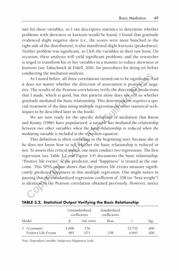
This definition is often confusing to the beginning user, because she or he does not know how to tell whether the basic relationship is reduced or not. To assess this critical matter, one must conduct two regressions. The first regression (see Table 3.2 and Figure 3.4) documents the basic relationship: “Positive life events” is the predictor, and “happiness” is treated as the outcome. This SPSS output shows that the positive life events measure significantly predicted happiness in this multiple regression. One might notice in passing that the standardized regression coefficient of .338 (or “beta weight”) is identical to the Pearson correlation obtained previously. However, notice
TABLE 3.2. Statistical Output Verifying the Basic Relationship
that I am using the unstandardized regression coefficient in the path model here rather than the beta weight because most associated computations involving the indirect effect in mediation use this type of coefficient, and this will be evident later when I describe the computation of Sobel’s z-score.
This step merely demonstrates in a regression format that we have a significant basic relationship. The next step is to perform a simultaneous inclusion regression in which the predictor (positive life events) and the mediating variables (gratitude) are both included in the analytical model as predictors of happiness. In essence, all we are doing is adding the mediating variable to the previous equation. Table 3.3 presents the results.
Notice that gratitude is a significant predictor of happiness and that positive life events, which previously was a significant predictor by itself, is now reduced in its strength as a predictor. The previous definition says that mediation occurs when the basic relationship is reduced when the mediating variable is added. Did it occur? If you compare the initial .338 beta weight with the subsequent .188 beta weight, or the initial .485 B with the subsequent B of .269, it certainly looks as though mediation occurred; that is, the basic relationship between the predictor and the outcome was reduced.
TABLE 3.3. Statistical Output of the Independent and Mediating Variables Predicting the dependent Variable
Unstandardized coefficients
Standardized coefficients
Model B Std. error Beta t Sig.
1. (Constant) Positive Life Events Gratitude Survey
So on the basis of these two regressions, can I assert that mediation occurred? Actually, I cannot. Who is to say that this reduction was significantly large enough to qualify as a statistically significant reduction? As it turns out, Sobel, a statistician, has come up with a way to determine whether it is sufficiently large. Sobel published a paper in 1982 that laid out a statistical test that researchers can use to verify whether the reduction is statistically significant or not. I should mention in this context that it is a test of the size of the indirect effect, that is, the amount of the basic relationship that “goes through” the indirect path from X to MedV to Y. The numerator is the estimate of the indirect effect, and the denominator is the standard error of this estimate. And it might help to be aware that the null hypothesis that the Sobel test is testing is a*b = 0, namely, that the size of the indirect effect is very small.
a*b z-value = (3.4)
2 2SQRT(b2*s + a2*sb)a
To make sense of this equation, you need to know (see Figure 3.5) that a refers to the unstandardized regression coefficient (the B, not the beta) for the path from X to the MedV, b refers to the unstandardized regression coefficient for the path from the MedV to Y in a simultaneous inclusion regression involving X and MedV as predictors of Y, sa refers to the standard error of the a path, and sb refers to the standard error of the b path.
Does anyone want to compute this equation by hand? Although I have hand-computed this equation dozens of times, I find it tedious to do. A great
Positive life events Happiness
Gratitude a b
c′
(sb)(sa)
fIgURE 3.5. Second model with specification of the indirect path with B’s and standard errors.
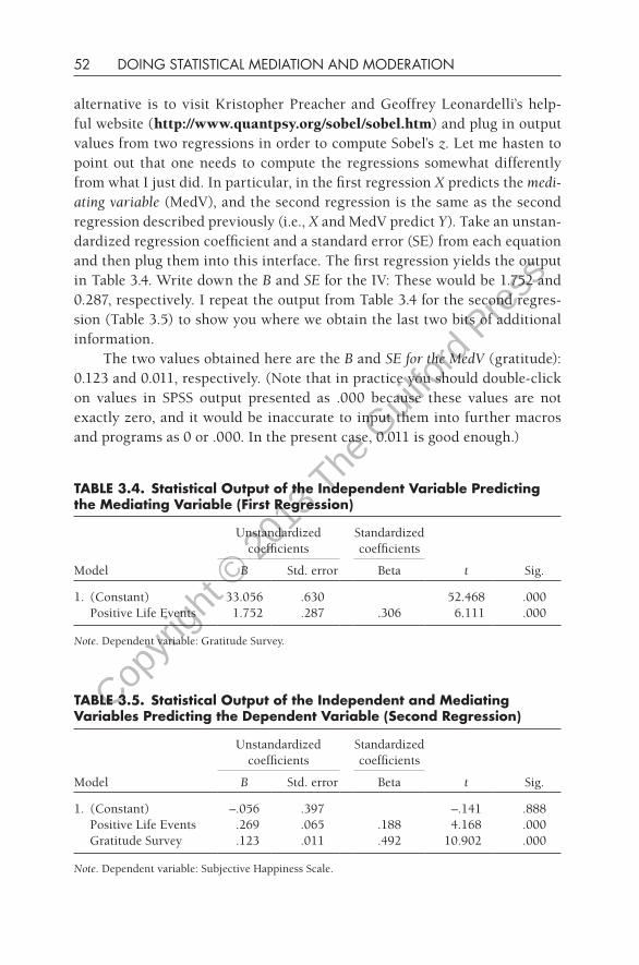
alternative is to visit Kristopher Preacher and Geoffrey Leonardelli’s helpful website (http://www.quantpsy.org/sobel/sobel.htm) and plug in output values from two regressions in order to compute Sobel’s z. Let me hasten to point out that one needs to compute the regressions somewhat differently from what I just did. In particular, in the first regression X predicts the mediating variable (MedV), and the second regression is the same as the second regression described previously (i.e., X and MedV predict Y). Take an unstandardized regression coefficient and a standard error (SE) from each equation and then plug them into this interface. The first regression yields the output in Table 3.4. Write down the B and SE for the IV: These would be 1.752 and 0.287, respectively. I repeat the output from Table 3.4 for the second regression (Table 3.5) to show you where we obtain the last two bits of additional information.
The two values obtained here are the B and SE for the MedV (gratitude): 0.123 and 0.011, respectively. (Note that in practice you should double-click on values in SPSS output presented as .000 because these values are not exactly zero, and it would be inaccurate to input them into further macros and programs as 0 or .000. In the present case, 0.011 is good enough.)
TABLE 3.4. Statistical Output of the Independent Variable Predicting the Mediating Variable (first Regression)
Now you have all of the necessary information. Go ahead and find this website and input these values. I assume that you did visit this site and correctly input the values. You should have obtained the output in Table 3.6.
Excellent! We now have a result. We have a significant Sobel z-value (the p-value, presented as 8e-8, is given in scientific notation, and it tells us that we move the decimal point eight positions to the left, that is, .00000008; as you can see, this value is hugely less than .05), and this result tells us that we have obtained a statistically significant mediation.
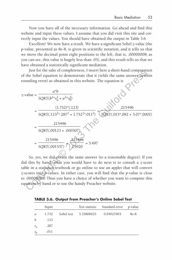
Just for the sake of completeness, I insert here a short-hand computation of the Sobel equation to demonstrate that it yields the same answer (within rounding error) as obtained in this website. The equation is
So, yes, we did obtain the same answer (to a reasonable degree). If you did this by hand, what you would have to do next is to consult a z-score table in a statistics textbook or go online to use an applet that will convert z-scores into p-values. In either case, you will find that the p-value is close to .00000008. Thus you have a choice of whether you want to compute this equation by hand or to use the handy Preacher website.
TABLE 3.6. Output from Preacher’s Online Sobel Test
Let me emphasize at this point that 0.215 is the “size of the mediated effect” or “size of the indirect effect.” It was obtained here by multiplying a by b, and note that these are the unstandardized regression coefficients, not the betas. Further, the value of 0.039 is referred to as the “standard error of the mediated effect.”
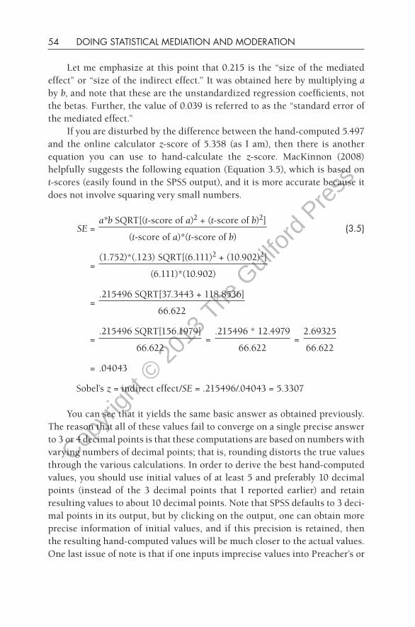
If you are disturbed by the difference between the hand-computed 5.497 and the online calculator z-score of 5.358 (as I am), then there is another equation you can use to hand-calculate the z-score. MacKinnon (2008) helpfully suggests the following equation (Equation 3.5), which is based on t-scores (easily found in the SPSS output), and it is more accurate because it does not involve squaring very small numbers.
a*b SQRT[(t-score of a)2 + (t-score of b)2]SE = (3.5)
Sobel’s z = indirect effect/SE = .215496/.04043 = 5.3307
You can see that it yields the same basic answer as obtained previously. The reason that all of these values fail to converge on a single precise answer to 3 or 4 decimal points is that these computations are based on numbers with varying numbers of decimal points; that is, rounding distorts the true values through the various calculations. In order to derive the best hand-computed values, you should use initial values of at least 5 and preferably 10 decimal points (instead of the 3 decimal points that I reported earlier) and retain resulting values to about 10 decimal points. Note that SPSS defaults to 3 decimal points in its output, but by clicking on the output, one can obtain more precise information of initial values, and if this precision is retained, then the resulting hand-computed values will be much closer to the actual values. One last issue of note is that if one inputs imprecise values into Preacher’s or
my macros, then the resulting values will reflect this imprecision. In practice, enter values at least to 5 decimal points, preferably to 10 decimal points.
Confidence Interval Information
It is useful to know whether the obtained indirect effect is statistically significant with the computation of a confidence interval (CI; these can be computed in addition to Sobel’s formula), and here is how to do this. Once you know the size of the estimate of the indirect effect and the SE (computed previously), you can insert these values into the following lower and upper CI equations and determine whether the range includes the value of zero or not (see Table 3.7). I use the SE determined from the t-score method, as I trust it more than the other method.
Putting all of this information together, one can say this: “The size of the indirect effect was found to be 0.215, SE = 0.04, with 95% CI values of 0.14 to 0.29. Because the CI did not include zero, one can conclude that this mediation result is statistically significant. Therefore, it seems that gratitude functioned as a significant mediator between positive life events and happiness.”
MacKinnon (2008) points out that an indirect effect computed from the product term (a*b) would more validly be evaluated with asymmetrical confidence limits (instead of 1.96 as in Table 3.7, they would be –1.6175 and 2.2540, respectively, for lower and upper limits, adjusting for the distribution of multiplied values). Recomputing these equations, I obtained the new values shown in Table 3.8.
Thus, by adjusting for a slight shift in the distribution caused by multiplying these two values together, the resulting CI boundaries move slightly upward. In the present case, both symmetrical and asymmetrical CIs yield
TABLE 3.7. Calculation of the Symmetrical 95% Confidence Interval
Estimate of indirect effect ± (95% CI coefficient × Standard error)
TABLE 3.8. Calculation of the Asymmetrical 95% Confidence Interval
Estimate of (Asym. 95% CI indirect effect ± coefficient × Standard error)
Lower limit .215496 – (1.62 × .0404)
.215496 – .065448
.150048
Upper limit .215496 + (2.25 × .0404)
.215496 + .09090
.306396
a significant result, but you are advised to use the asymmetrical confidence limits when you obtain the indirect effect by multiplying a by b. And one last issue: The 95% CI is standard because most users adopt the traditional p < .05 cutoff rule, but of course one may adopt different values. A symmetrical 99% CI (p < .01) would use a value of 2.575 instead of 1.96.
For more information about the derivation of asymmetrical confidence limits for mediated effects, read MacKinnon, Fritz, Williams, and Lockwood’s (2007) article on PRODCLIN, a stand-alone program devoted to this topic. The program allows the user to input values for a and b, their standard errors, the correlation between a and b, and the Type I error rate. The program then generates the asymmetric confidence limits, which can be used to identify whether the indirect effect is statistically significant or not. You may also be interested in an R program named RMediation, which can perform similar functions (Tofighi & MacKinnon, 2011).
KNOWLEdgE BOx. Controversy: Calculation of Whether Significant Mediation Has Occurred
The approach described in this chapter is based on the original Baron and Kenny formulation set down in 1986, and I have focused on it simply because it seems to have been adopted by the largest number of people and the widest range of disciplines. It is not the only way to compute whether significant mediation has occurred, however.
Let me be clearer on this point. The so-called “Baron and Kenny causal steps model” enunciated herein is the simplest approach; if the beta weight for the basic relationship goes down when the MedV is included in the regression equation, then significant mediation is assumed to have happened. Many researchers and statisticians are dissatisfied with this method
because (as I noted previously), it is not clear how much of a decrease is necessary.
That’s where Sobel’s test comes in. Baron and Kenny described the use of Sobel’s z-test in their article, and many (but not all) researchers have adopted this additional criterion in order to be more certain that the observed decrease is “statistically significant.” This approach is the basic level of mediation analysis that I want to see from a researcher.
But it is not the final answer. As MacKinnon and colleagues (e.g., Fritz & MacKinnon, 2007; MacKinnon et al., 2002) have pointed out, there are many other options, including the Aroian computation (see Kris preacher’s website for this computation), the joint significance test (determining whether both the a and b paths [X to MedV and MedV to Y] are significant), various confidence limits approaches (see MacKinnon, Lockwood, & Williams, 2004), and a number of different bootstrapping methods.
Which is best? Considerable controversy still exists on this issue, but it seems that the prevailing direction of movement is away from multipleregression-based mediation analyses toward bootstrapping methods (see Kenny, 2008; MacKinnon, Fairchild, & Fritz, 2007). So why am I teaching Sobel’s z-test approach here? The answer is that informed users need to begin with this basic approach, learn it thoroughly, and, when they have acquired sufficient statistical knowledge and expertise with various statistical platforms (e.g., SEM, multilevel modeling, bootstrapping), then they will naturally move on to the more powerful techniques. (you will find a description of bootstrapping in the next chapter, which will take you to this next level, if you are interested and committed.) This book is written to acquaint you with the history and the basics of both mediation and moderation and hopefully to prepare you for a career-long exploration of new developments in these areas over time.
Strength of Indirect Effect
Here is an additional question for you to consider: How strong of a mediational effect did you obtain? You are able to answer that it was statistically significant, but you are not able to say whether the amount of mediation (indirect effect = 0.215) was small, medium, or large. Baron and Kenny (1986) say that perfect mediation is obtained when the basic relationship is reduced to zero, and significant mediation is obtained when the Sobel z-value is significant but the basic relationship is not reduced to zero. As noted in Chapter 2, Baron and Kenny acknowledged that perfect mediation is very unlikely in the social sciences, in which probabilistic data are gathered. That leaves considerable ambiguity about the size of the effect. MacKinnon (MacKinnon, 2008;
MacKinnon, Warsi, & Dwyer, 1995) argues that we need to have a metric for the ratio between the direct and indirect effects because it would clarify the issue about the strength of the mediation effect.
MacKinnon, in his book on mediation (2008), states that there are three different (but related) ways to measure the effect size of the mediated effect: (1) ratio and proportion measures; (2) R2 measures; and (3) standardized effect measures. The first approach computes various ratios between different effects. For example, Sobel (1982) suggested that one could divide the indirect effect by the direct effect; in the present case, it would be 0.215/0.269 = 0.80. Another ratio computation is to determine the proportion of the total effect that is mediated: [1 – (c′/c)] or [ab/c], which in the present case would be 0.44. (See Kenny’s discussion of these two ratios at http://davidakenny. net/cm/mediate.htm.) Problems arise, however, if one has both negative and positive estimates. Absolute values are recommended for use in these equations. The second approach, R2 measures, requires the computation of the amounts of variance in Y explained by X alone (variance of the direct effect) and by X and MedV together (allowing identification of the variance of the indirect effect). The most useful index, perhaps, from this approach is the proportion of the variance of the indirect effect to the variance of the total effect. In the present case, it is 0.728 (see the upcoming section on semipartial correlations for instructions about how to compute this ratio). A ratio of 0.73 suggests that almost three-fourths of the variance in the total effect is composed of the indirect effect, a sizable proportion. And the third and last approach yields an effect size in standardized units, dividing the indirect effect by the standard deviation of the DV. In the present case, this is 0.215/1.344 = 0.159. Which of these indices is the best? My view is that they all tell us something useful about the relationships in the mediational triangle, but they illuminate different aspects of the mediational triangle. I think two indices are particularly illuminating: (1) the ratio of the indirect effect to the total effect based on standardized regression coefficients and (2) the same ratio using R2 measures. On the other hand, these two methods yield differing estimates of the “size of the indirect effect,” so one must be careful in explaining which method one is reporting in a given context.
It is probably helpful to point out at this juncture that recent work by Preacher and Kelley (2011) suggests several more effect size indices that should be considered by the research community. One new effect size index is an index based on residuals; in particular, it is based on the amount of variance explained in both the mediator and the outcome. The other new effect size index assesses the indirect effect as a proportion of the maximum possible indirect effect that could have been obtained given the variables
involved. Although these are new developments, these indices are promising and deserve attention in future work.
I created a website in 2004 that I designed to provide a graphical depiction of the mediational triangle to the user and to provide information on effect sizes. Let us consider output generated by MedGraph on the present mediational pattern, and in this fashion you can see how these effect size values are generated. Go to http://www.vuw.ac.nz/psyc/staff/paul-jose/files/ medgraph/medgraph.php and input the necessary output values into Med-Graph. You will notice that it asks for more information than the previous website does, and the reason for this is that these other sources of information are needed to create a full graph or figure of the mediational triangle. In particular, you need to provide the correlation matrix, the size of the sample, the B’s and standard errors stipulated previously, and the altered betas in the final regression. If you input all of these values, you will obtain a figure that looks like Figure 3.6.
My intent was to create a website that would provide the user with more information than just Sobel’s z-score so that he or she would be able to make a more appropriate interpretation of the finding. Beyond Sobel’s z-score, this website also reports the associated significance level and the 95% symmetrical CI. Also in the figure, output provides information to allow the user to determine the strength of the mediational effect in three ways. The first is based on unstandardized regression coefficients, and the total effect refers to the original bivariate relationship between the IV and the DV, 0.485 in this case. (You should take absolute values of these estimates, rendering negative numbers positive.) The total effect is partitioned into two components: direct and indirect effects. The direct effect is the regression coefficient after inclusion of the MedV, 0.269 in this case, and the indirect effect is the total effect minus the direct effect, 0.215 in this case. The indirect/total ratio computed on the basis of unstandardized coefficients refers to 0.215/0.485, or 0.443. The ratio value varies from 0 to 1 and tells the user how much of the original basic relationship is explained by the indirect effect; in this case it turned out to be somewhat less than half (i.e., 44%).
The second column reports the same values in terms of standardized regression coefficients (see also the values reported in the mediational triangle, which are the same). You should notice that the indirect/total ratio (0.150/0.338 = 0.443) is identical, whether one computes it with unstandardized or standardized coefficients.
The last set of values report the R2 estimates (based on variances), which allows a different (but related) way to identify the size of the indirect effect. These values are generated by using the semipartial correlations of the predictor variable and MedV with the outcome. In addition to other statistical output described before, MedGraph asks the user to input “part correlations” (also known as semipartial correlations) generated by the hierarchical regression analysis described earlier in this chapter. This analysis enters the predictor on the first step and then adds the MedV on the second step. The resulting semipartial correlations are used in several simple computations (see pp. 82–86 later in this chapter that describe these conversions) that yield these three reported values in the MedGraph output. It is important to notice—and it is fairly obvious—that these values differ from the estimates of effect sizes generated by standardized regression coefficients, but let me assure the reader that they are based on the same statistical outputs. The values in the left column are perhaps easier to understand because they refer to relative sizes of regression coefficients, whereas the values in the right column are more opaque because they are based on relative amounts of explained variance in the outcome, which are not obvious
and apparent. I have designed MedGraph to report all three types because all are valid ways to examine the mediational results, and I leave it to the user to decide which of these two approaches best suits his or her particular mode of explanation.
And last, below these outputs is the graph of the mediational triangle, and it succinctly tells the researcher everything that he or she needs to know about the dynamic interplay of these variables. I suppose the graph is not entirely necessary, but I am a very visual person, and I like to see the entire mediational triangle laid out in its entirety to facilitate my understanding of what the result means. It forces the researcher to double-check that he or she has entered the data correctly (which does not always happen).
Did the Multiplicative Rule Work?
Remember that I said that a*b = c – c′? How did that work out? Focusing on the unstandardized regression coefficients, the numbers I obtained are: 1.752 * 0.123 = 0.215 and 0.485 – 0.269 = 0.216, which are close, given rounding errors. The same computations with standardized regression coefficients are: 0.306 * 0.492 = 0.150 and 0.338 – 0.188 = 0.150. Thus the multiplicative rule works regardless of whether you use unstandardized or standardized coefficients, but it should be clear that the two methods yield different absolute values for the size of the indirect effect. I have focused on computing the indirect effect with unstandardized regression coefficients because this is the customary way to derive it and because this value is used in other equations (such as computation of the confidence intervals). I showed you the numbers generated by the standardized coefficients only to point out that the indirect/ total ratio is identical for these two sets of numbers.
Interpretation of the Result
I think we are ready to interpret the outcome. The results generated by Med-Graph tell us that gratitude acted as a significant mediator between positive life events and happiness. The statistical output, after being transformed by several equations, tell us that the basic relationship was significantly reduced by the introduction of a third variable (unstandardized indirect effect = 0.215; ratio of indirect/total = 0.44). The ratio tells us that the path through the mediating variable accounted for almost half of the basic relationship between the predictor and the outcome, and the R2 estimate of the indirect effect tells us that about three quarters of this relationship was explained by the indirect effect.
How might we interpret this result? I would say the following. “The results show that if someone experiences a high level of positive life events, then he or she is likely to report greater happiness. This relationship can be partially explained by detailing the involvement of gratitude. In essence, individuals who reported higher levels of positive life events reported feeling more grateful, and, in turn, grateful individuals reported higher levels of happiness.” These results make intuitive sense, and I am not aware of any published report that includes all three of these particular constructs in this particular fashion, so this may be a unique finding. Nevertheless, researchers (Emmons & McCullough, 2003; Watkins, Woodward, Stone, & Kolts, 2003) have noted that gratitude is positively associated with happiness, one link in this triangle.
The estimates of direct and indirect effects tell us how strongly this mediator operated. In this particular case, the indirect effect was relatively large compared with the direct effect. The ratio tells us that almost half (in the case of regression coefficients) of the effect of positive life events on happiness was “explained by” the intervening variable of gratitude. In other words, a considerable amount of the shared variance between positive life events and happiness was explained by the indirect route through gratitude. Researchers say that mediation tells us about the “operating mechanism” that exists among three variables, and this interpretation is relevant here in that we can say that we have discovered that gratitude seems to explain a significant part of the relationship between positive life events and happiness.
AN ExAMPLE Of MEdIATION WITH ExPERIMENTAL dATA
The previous example was based on survey data collected at one point in time (often called “concurrent”), and some of you will have data of this type. However, in the social and physical sciences, a researcher often will have experimental or quasi-experimental data. MacKinnon has written extensively about this subject (2008; MacKinnon & Dwyer, 1993), and reading his various papers will provide a more detailed treatment of this topic than I can present here, but I would like to briefly touch on this method. The two chief differences from the mediation example presented here are:
1. The IV is often a dichotomous categorical variable that represents the enactment of an intervention.
2. Temporal order of the variables allows for an unambiguous placement of the variables within the mediational triangle.
On the first point, I noted at the outset of this chapter that an experimental manipulation will usually yield a categorical dichotomous variable in which 1 = experimental group and 0 = control group. The values should be 0 and 1, not 1 and 2, because this variable is technically a dummy code (see a fuller explanation concerning dummy codes in Chapter 5). If we create more than two groups, as can happen when we are manipulating dosage levels of an intervention, then the IV will be more complex and can be composed of several dummy codes. In the present case, I keep it simple and focus on a single dichotomous categorical IV.
On the second point, let me note that when we have three concurrent variables, as in the previous mediation example, we can juggle the order of the variables in the three slots in the mediational triangle; but when we have experimental data, the design constrains the placement of variables. Presumably the IV is enacted at the outset of the study, so it would naturally be located in the leftmost slot. The mediation variable is obtained subsequent to the manipulation and would come next in order; and finally, the outcome, usually temporally obtained last, would fall into the final slot. Sometimes the researcher measures the mediating and outcome variables simultaneously at the end of the study, and this may create problems (see Baron & Kenny, 1986, on this point).
Helpful Suggestion: If you access the dataset titled “experimental mediation example.sav,” you can perform the analyses that I report next.
The present dataset came from a quasi-experimental study of resilience in 13-year-old adolescents conducted by one of my PhD students, Olivia Notter. She enacted a positive psychology-based program named PAL that sought to orient these teenagers to identify strengths, savor pleasant experiences, find flow in their lives, and practice feeling gratitude about the positive things in their lives. We predicted that students who participated in the PAL program would, as a consequence, report greater life satisfaction. Further, we expected to find a mediational pathway through increased gratitude that would lead to greater life satisfaction. The predicted mediational pattern is depicted in Figure 3.7.
We screened a large group of 13-year-olds and selected individuals with mildly to moderately elevated depression scores (i.e., individuals who were “at risk”). We solicited students in this range to volunteer for a program to help with living skills. Those who volunteered were randomly assorted into either the experimental or the control group. Pretest depression scores
64 DOING STATISTICAL MEDIATION AND MODERATION
indicated that the two groups did not differ significantly. Due to the time-consuming and extensive nature of the program, the two groups ended up with relatively small numbers (compared with other datasets described in this book). The experimental group constituted 38 teenagers, and the control was composed of 30 teenagers. The program ran for 12 weeks, 1 hour per week, and at the conclusion of the program (time 2) various measures were taken, including self-reported gratitude. Life satisfaction was assessed at this point as well as 6 months later, at time 3. We used the equations described earlier to conduct the analyses:
The correlations and the two regression equations yielded the outputs presented in Tables 3.9, 3.10. 3.11, and 3.12 and in Figure 3.8. Selecting values from these outputs, one can compute Sobel’s test by hand in this fashion:
TABLE 3.11. Statistical Output for the Relationship between the Independent Variable and Mediating Variable of the Experimental Mediation Example (first Model)
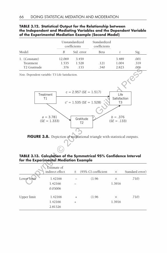
TABLE 3.12. Statistical Output for the Relationship between the Independent and Mediating Variables and the dependent Variable of the Experimental Mediation Example (Second Model)
Taken together, these results tell me that I obtained significant mediation with these three variables across this period of time. The interpretation would be:
“Support was found for the hypothesis that gratitude significantly mediated between the treatment effect of the PAL program and resulting life satisfaction 6 months after the conclusion of the program. Specifically, a measurable treatment effect was greater gratitude among the experimental group participants noted at the conclusion of the 12-week program, and this difference differentially predicted greater life satisfaction 6 months later. The mediational analysis yielded a Sobel z-score of 2.003, p = .045, asymmetrical 95% CI was .03 to 2.81. The standardized effect size indicated that about 48% of the total effect of the treatment on resulting life satisfaction was explained by the indirect effect through gratitude.”
AN ExAMPLE Of NULL MEdIATION
According to Baron and Kenny, one should not examine a mediation triangle in which at least one of the three relationships is statistically nonsignificant. According to this rule, the easiest example of null mediation that you will run across is a dataset in which at least one of the three preconditions is not met. (People have questioned whether this is a sound procedure, though, so see the upcoming section “Suppressor Variables in Mediation” for a reexamination of this assumption.)
However, there is a slightly more interesting example of null mediation—if there is such a thing—in which the three variables display significant zero-order correlations with each other but Sobel’s z-score is nonsignificant. Following is an example of this latter type of no (or null) mediation that I found in a dataset supplied to me by my colleague, Dr. Taciano Milfont, in my home institution (i.e., the School of Psychology, Victoria University of Wellington, New Zealand). He has described these variables and this dataset (Milfont, Duckitt, & Wagner, 2010), but for obvious reasons he did not describe this particular relationship—I had to go looking for it to find it.
Helpful Suggestion: Just as I suggested earlier with basic mediation, if you would like to analyze the present dataset and conduct the following analyses on it as you go through this section, find and download “null mediation example.sav.”
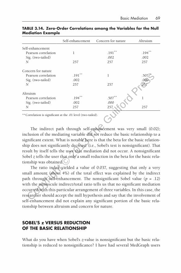
Taciano is interested in how personal values inform and affect attitudes and behaviors concerned with preservation and protection of the environment. The hypothesis to be tested was that the effect of altruism on environmental values (the degree to which individuals endorsed items measuring unity with nature, protecting the environment, and respecting the Earth, taken from the Schwartz Value Scale; Schwartz, 1994) would be mediated by the value of self-enhancement. In essence, one’s general altruism should predict concern for nature, and it might be mediated by a general orientation toward doing things to enhance one’s own self. I thought this might make sense insofar as an altruistic person might be motivated by self-enhancement to be concerned about nature. The researchers obtained data from three countries (South Africa, New Zealand, and Brazil), but in this particular case I focused only on the South African group (N = 257). I proceeded to compute the regressions and obtain the MedGraph result (see Figure 3.9). The correlation matrix that I obtained is presented in Table 3.14.
Type of Mediation Null Sobel z-value 1.537598 significance p =.124147 Standardized coefficient of Altruism on Concern for Natu re
Concern for nature Pearson correlation .191** 1 .507**
Sig. (two-tailed) .002 .000 N 257 257 257
Altruism Pearson correlation .194** .507** 1 Sig. (two-tailed) .002 .000 N 257 257 257
**Correlation is significant at the .01 level (two-tailed).
The indirect path through self-enhancement was very small (0.02); inclusion of the mediating variable did not reduce the basic relationship to a significant extent. What is notable here is that the beta for the basic relationship does not significantly decrease (i.e., Sobel’s test is nonsignificant). That result by itself tells the user that mediation did not occur. A nonsignificant Sobel z tells the user that only a small reduction in the beta for the basic relationship was obtained.
The ratio index yielded a value of 0.037, suggesting that only a very small amount (about 4%) of the total effect was explained by the indirect path through self-enhancement. The nonsignificant Sobel value (p = .12) with the minuscule indirect/total ratio tells us that no significant mediation occurred with this particular arrangement of three variables. In this case, the researcher should accept the null hypothesis and say that the involvement of self-enhancement did not explain any significant portion of the basic relationship between altruism and concern for nature.
SOBEL’S z VERSUS REdUCTION Of THE BASIC RELATIONSHIP
What do you have when Sobel’s z-value is nonsignificant but the basic relationship is reduced to nonsignificance? I have had several MedGraph users
raise this issue. In essence, what happens is that the beta for the basic relationship is initially statistically significant, but when the mediating variable is included, the basic relationship decreases to nonsignificance. At the same time, Sobel’s z-test yields a nonsignificant z-value. According to some people’s thinking (based on reading Baron and Kenny, I think), the reduction of the basic relationship to nonsignificance suggests that one has obtained significant mediation. However, I think that most mediation cognoscenti (that means “people in the know”) would agree that the Sobel test takes precedence in this case: if Sobel’s z is nonsignificant, then one has obtained null mediation. End of the story.
This situation is usually obtained when the original basic relationship is barely significant, for example, p = .04, and although the subsequent Sobel test might show that the mediating variable explains a small portion of the basic relationship—for example, the p-value for the Sobel test might be .08— Sobel’s z will not be sufficiently large to obtain that all-important “p less than .05” outcome. My advice in this situation is to acknowledge the nonsignificant Sobel test and admit that null mediation was obtained. A result such as this can be frustrating to the researcher, and she or he may be inclined to ignore Sobel’s z result, but its use has been adopted into general practice now, and I do not think it can be ignored. The researcher may wish to report this result as “suggestive of a possibility that a trend might have happened” or such, but there are some statisticians who would say that even that is too bold. My advice: Be honest about what you found. Do not overinterpret the result, even if it is very enticing for you to find a significant result.
SUPPRESSOR VARIABLES IN MEdIATION
Can the strength of the basic relationship increase when the mediating variable is included? Yes. Occasionally we find the paradoxical situation in which we obtain significant mediation (as determined by the Sobel test) but the beta for the basic relationship actually goes up when the mediating variable is included. Following is a case in point. I am again using the dataset provided by my colleague Taciano Milfont, which was described in the previous section on “null mediation.” Although he has published a report from these data (see Milfont et al., 2010), he did not report this particular aspect of the data. I found this relationship when I began examining the mediational relationships among the variables. As deep background, you may wish to read their report to obtain a greater understanding of what these variables measure and why I might have obtained a suppressor effect in this case. They obtained
data from three countries (South Africa, New Zealand, and Brazil), and the present analyses were performed only on the South African data.
Helpful Suggestion: Find the dataset “suppressor mediation example.sav” if you would like to analyze this dataset, and conduct the following analyses on it as you go through this section.
In this case, altruism is the predictor variable (the degree to which individuals endorsed items measuring a desire for equality, a world at peace, and social justice, taken from the Schwartz Value Scale; Schwartz, 1994), the mediating variable is self-enhancement (the degree to which individuals endorsed being wealthy, wielding authority, and being influential, also taken from the Schwartz Value Scale), and the outcome is a summed score of generalized environmental attitudes (assessed by the Milfont & Duckitt Environmental Attitudes Inventory, 2010). The basic correlations are presented in Table 3.15. Right away the astute researcher should be able to note that something is out of the ordinary. There is an implicit logic to correlation matrices in that variables that are correlated in a positive direction with each other should generalize that direction of correlation to a new variable. In other words, if X and Y are positively correlated with each other, then a third vari-
TABLE 3.15. Zero-Order Correlations for the Variables in the Suppressor Variable Example
General Environmental Altruism Self-enhancement Atts
able Z should be “consistent” and correlate in the same direction with both X and Y. This pattern is not found in the previous example. Altruism and self-enhancement are positively correlated, but when I add the third variable, I find that although altruism is positively correlated with general environmental attitudes, surprisingly self-enhancement is negatively correlated with general environmental attitudes.
In this case I consider altruism to be my predictor, self-enhancement to be my MedV, and general environmental attitudes to be my outcome. I run my mediational analysis, and Figure 3.10 presents what I obtained. Hmmm, that’s interesting. MedGraph tells me that I have obtained significant mediation, yet the basic relationship becomes stronger. And note that the direct, indirect, and total effects (and ratio) do not make sense because the indirect effect has a different sign than the direct effect. So what is going on here? What we have here is a suppressor variable (Conger, 1974; Darlington, 1968; Horst, 1941; Krus & Wilkinson, 1986; Paulhus, Robins, Trzesniewski, & Tracy, 2004). A suppressor variable is defined differently by different authors, but Conger defines it as “a variable that increases regression weights and, thus, increases the predictive validity of other variables in a regression equation” (Conger, 1974, pp. 36–37). One can notice that both the X-to-Y and the
Type of Mediation Significant Sobel z-value -2.553226 significance p = .010673 Standardized coefficient of Collectivism on Depression
MedV-to-Y relationships are increased here. Several types of suppressor variables have been identified (see Krus & Wilkinson, 1986, or Gaylord-Harden, Cunningham, Holmbeck, & Grant, 2010), but this discussion is not pursued here because of a concern for space.
Some authors argue that this phenomenon reveals spuriousness, that is, false or misleading correlations, but some writers (and I agree with this point of view) think that these relationships may reveal important information about the ways in which these variables are related. For example, in the mediational triangle in Figure 3.10 we see that self-enhancement has a paradoxical (enigmatically termed “quasiparadoxical” by Cohen & Cohen, 1975) relationship with the other two variables. Altruism positively predicts self-enhancement, suggesting that an altruistic person is enjoying some self-enhancing aspect of being altruistic (“Aren’t I a good person for helping out others?”), but self-enhancement, in turn, is a negative predictor of general environmental attitudes, suggesting that a person high in self-enhancement is relatively uninterested in helping the environment. These two relationships suggest that there is a counterintuitive indirect path between the X and Y relationship—namely, that being altruistic is positively predictive of having more positive environmental attitudes through the intervening variable of self-enhancement.
Some people think that suppressor relationships are false and spurious, and maybe some are, but I do not think that there is anything false or spurious about the present set of relationships. I think that they make perfect sense, in that self-enhancement is related to altruistic impulses in some people, and this psychological dynamic seems to work against a person having more proenvironment attitudes. I would suggest in the present case that this obtained finding is potentially valuable because it points out the danger of making altruism a salient reason for people to care for the environment: Some may espouse altruistic views to enhance their own sense of self, but this strategy might not increase positive environmental attitudes. By the way, these data were concurrent, taken at one point in time, and the present set of findings cries out for a longitudinal study to be done to probe the causal relationships hinted at by this mediation result.
In sum, I think that evidence of a suppressor variable is a marvelous motivation to probe the relationships more closely and identify the hidden currents swirling below the surface. I recommend that if and when you find evidence of a suppressor effect you take the opportunity to examine the relationships more closely in order to unpack the reasons that the X-to-Y beta weight increased. In my experience one is more likely to find a suppressor
effect when one obtains either one or three negative correlations (in the case of three-variable mediation), when the researcher is using a large sample size, and when the measures involved are composed of multiple items.
INVESTIgATINg MEdIATION WHEN ONE HAS A NONSIgNIfICANT CORRELATION
Is it feasible to examine mediation when one does not have three significant relationships? As it has been laid out by Baron and Kenny, the dogma (repeated by me at the beginning of this chapter) is that one must have three significant correlations before one can examine mediation. However, I also noted that this stipulation is controversial, and MacKinnon (2008), among others, has argued that mediation can be found in triads of variables in which the X-to-Y relationship is not statistically significant.
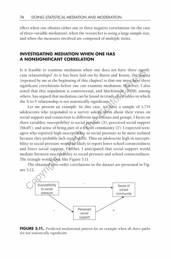
Let me present an example. In this case, we have a sample of 1,774 adolescents who responded to a survey asking them about their views on social support and connection to different institutions and groups. I focus on three variables: susceptibility to social pressure (X), perceived social support (MedV), and sense of being part of a school community (Y). I expected teenagers who reported high susceptibility to social pressure to be more isolated because they probably lack social skills. Thus an adolescent high in susceptibility to social pressure would be likely to report lower school connectedness and lower social support. Further, I anticipated that social support would mediate between susceptibility to social pressure and school connectedness. The triangle would look like Figure 3.11.
The obtained zero-order correlations in the dataset are presented in Figure 3.12.
fIgURE 3.11. Predicted mediational pattern for an example when all three paths are not statistically significant.
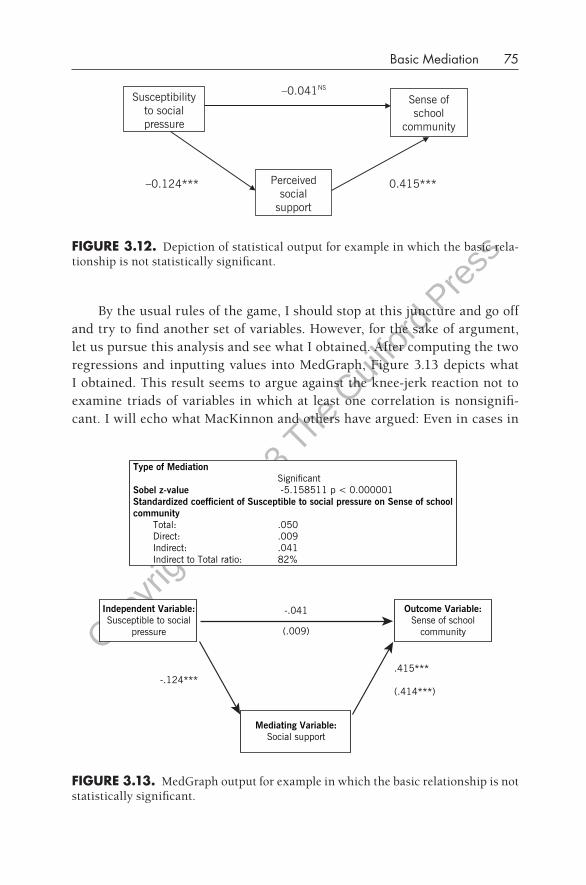
By the usual rules of the game, I should stop at this juncture and go off and try to find another set of variables. However, for the sake of argument, let us pursue this analysis and see what I obtained. After computing the two regressions and inputting values into MedGraph, Figure 3.13 depicts what I obtained. This result seems to argue against the knee-jerk reaction not to examine triads of variables in which at least one correlation is nonsignificant. I will echo what MacKinnon and others have argued: Even in cases in
fIgURE 3.12. Depiction of statistical output for example in which the basic relationship is not statistically significant.
Susceptibility to social pressure
Sense of school
community
Perceived social
support
–0.124*** 0.415***
–0.041NS
fIgURE 3.13. MedGraph output for example in which the basic relationship is not statistically significant.
Type of Mediation Significant
Sobel z-value -5.158511 p < 0.000001 Standardized coefficient of Susceptible to social pressure on Sense of school community
Total: .050 Direct: .009 Indirect: .041 Indirect to Total ratio: 82%
which one obtains a nonsignificant relationship, significant mediation might be found. In my experience, significant mediation is sometimes found in cases in which the X-to-Y relationship (c) is weak but the a and b links are strong (as in the preceding case).
You have now seen a case in which three significant correlations did not yield significant mediation (pp. 67–69), juxtaposed against this example in which significant mediation was obtained in a case in which a nonsignificant correlation was manifested in the mediational triangle. These examples should highlight to you that significant mediation is likelier to be found in cases in which the a and b links are strong, and it is likelier not to be found in cases in which either (or both) of the a and b links are weak.
UNdERSTANdINg THE MATHEMATICAL “fINE PRINT”: VARIANCES ANd COVARIANCES
I have found that it is easier to teach students how to conduct mediational analyses than it is to teach them how to make clear and unambiguous interpretations of the mediational findings. And one of the murky issues that students typically struggle with is the matter of what the indirect effect actually measures. I tell them helpful things such as “Well, the size of the indirect effect tells you the amount of variance in the total effect left over after you take out the direct effect.” The point I have gotten to now is to say “You know, you need to learn the mathematical stuff underlying the computations of hierarchical regressions.” And then I begin with Venn diagrams to ease them into the process. If you are interested in learning about some of the underlying foundation for mediational analyses, then I would recommend that you try to make it through the rest of this chapter, because I think that learning this material will make you a more informed user of mediation, and it will enable you to make clearer interpretations of your findings.
Before We get to Venn diagrams: Learning about Variances and Covariances
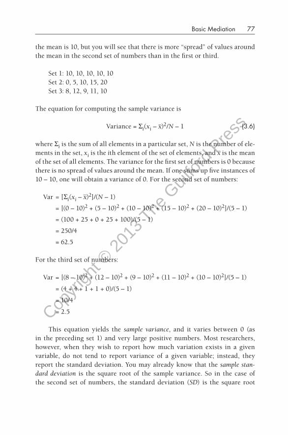
I think it might be useful to digress for a brief journey into the world of variance and covariance for a moment, because many people (including seasoned researchers, if truth be told) do not precisely understand what these terms mean. Here is a definition of variance: “the total amount of distribution of obtained values around the mean.” In the three following sets of numbers,
the mean is 10, but you will see that there is more “spread” of values around the mean in the second set of numbers than in the first or third.
Set 1: 10, 10, 10, 10, 10 Set 2: 0, 5, 10, 15, 20 Set 3: 8, 12, 9, 11, 10
The equation for computing the sample variance is
Variance = Si(xi – x)2/N – 1 (3.6)
where Si is the sum of all elements in a particular set, N is the number of elements in the set, xi is the ith element of the set of elements, and x is the mean of the set of all elements. The variance for the first set of numbers is 0 because there is no spread of values around the mean. If one sums up five instances of 10 – 10, one will obtain a variance of 0. For the second set of numbers:
This equation yields the sample variance, and it varies between 0 (as in the preceding set 1) and very large positive numbers. Most researchers, however, when they wish to report how much variation exists in a given variable, do not tend to report variance of a given variable; instead, they report the standard deviation. You may already know that the sample standard deviation is the square root of the sample variance. So in the case of the second set of numbers, the standard deviation (SD) is the square root
of 62.5, or 7.91, and in the case of the third set of numbers, it is the square root of 2.5, or 1.58.
Let us turn to covariance now. Covariance is an index of the degree to which two variables covary, or are related to each other. That sounds a lot like a correlation, so it is important to detail how these two constructs are similar and different. They are mathematically related, so it will probably be instructive to define each before we move on. Here is the usual definition of covariance in equation form:
Where x and y are the means of two variables:
S(xi – x)(yj – y)Cov(x, y) = (3.7)
N – 1
Using the second and third sets of values identified earlier, we have the values in Table 3.16 to consider. The sum of the products, 15, is divided by N – 1 (i.e., 4), which yields a covariance of 3.75. This result by itself is not very illuminating, but let’s move on to correlation now.
A definition of correlation, jumping off from the previous derivation of a covariance, is the following:
Cov(x,y) rx,y = (3.8)
s sx y
This equation is not meant to be daunting, and in fact it’s quite simple. What it means is that the correlation (r is the Greek letter rho) between variable x and variable y is equal to the covariance between two variables divided by the product of the two SDs (s is the Greek letter sigma, which commonly rep-
TABLE 3.16. Calculation of Covariance
xi – x yi – y Products xi yi
Subj. 1 0 8 –10 –2 20
Subj. 2 5 12 –5 2 –10
Subj. 3 10 9 0 –1 0
Subj. 4 15 11 5 1 5
Subj. 5 20 10 10 0 0
Mean 10 10 S = 15
Standard SQRT(62.5) = 7.91 SQRT(2.5) = 1.58 deviation
resents the SD). What this conversion accomplishes is to place the obtained values for correlations between the values of +1.0 and –1.0, thereby putting them on a metric that is easy to understand and appreciate. Most beginning statistics students readily grasp that positive correlation values indicate that things go along together, that negative correlation values indicate that things go in opposite directions, and that values near zero indicate that things are not associated very much at all. In the case given here, the covariance (3.75) is divided by the product of the two SDs (7.91 * 1.58 = 12.4978), which yields a correlation of .30. Most of us can understand how these two columns of numbers are related to each other with a correlation of .30 better than we can if we are told that they manifest a covariance of 3.75. But it is important to realize that the correlation is merely the covariance divided by the product of the two SDs.
Let’s consider a larger dataset. In this case I’ve correlated two variables, individualism and collectivism. Collectivism is the tendency to value one’s participation in groups and collectives and to be interdependent with others, and, in contrast, individualism describes the tendency to value competition, self-reliance, and independence (see Triandis, 1995). The analysis I requested yielded a covariance value of –.017 between individualism and collectivism in a sample of about 1,900 New Zealand adolescents. If I reported this statistic in a paper, most readers would be confused and would want to know what the Pearson correlation value was. One can see in Table 3.17 that the correlation is –.05, and with a sample of this size, this correlation is deemed to be statistically significant at p < .05, although it is obviously not very strong.
TABLE 3.17. Example of Correlation and Covariance between Individualism and Collectivism
Individ. Collect.
Individ. Pearson correlation 1 –.050* Sig. (two-tailed) .029 Covariance .417 –.017 N 1921 1921
Collect. Pearson correlation –.050* 1 Sig. (two-tailed) .029 Covariance –.017 .288 N 1921 1921
*Correlation is significant at the .05 level (two-tailed).
TABLE 3.18. descriptive Statistics of Individualism and Collectivism
N Mean Std. Deviation Variance
Individ. 1921 3.0013 .64574 .417
Collect. 1921 3.7967 .53693 .288
Valid N (listwise) 1921
I have also appended descriptive statistics (see Table 3.18) for the two variables in question. SPSS generated the variance and SDs of both variables, and these are reprinted in Table 3.18. You may notice a curious inconsistency between these two tables of findings. The covariance of individualism is reported to be .417 in Table 3.17, and the variance of the same variable is reported to be .417 in Table 3.18. So which is it? The answer is that the covariance of a variable with itself is known as the variance. It is customary to refer to the variance of a variable by itself but to covariances among pairs of variables.
What does all of this have to do with mediation? I want to make sure that you understand what the Venn diagrams in the next subsection depict as I go through this explanation. In essence, the circles represent variances of variables, and the graphical overlap between two variables defines the size of the covariance between any two variables.
graphical depiction of Mediation with Venn diagrams
Now that we have a clearer idea of what covariance, correlation, and variance are, we can now delve into the illuminating world of Venn diagrams. John Venn, a British philosopher and mathematician, introduced his system of diagrams in 1881 to illustrate set theory, that is, making clear distinctions about membership of unique or shared elements among sets. More than 100 years later, we are still using his invention to good effect. Venn diagrams are a good way to understand the various strengths of correlation, and Figure 3.14 presents four depictions of different-sized correlations.
Now we are ready to depict mediations, which require three variables. There are essentially two types of these: null and significant mediations. We begin with a typical example of significant mediation based on the example given at the outset of this chapter. We assume that the relationship between positive life events and happiness described earlier would look something like Figure 3.15, which depicts a moderate relationship. The area of overlap represents the shared variance between these two variables, and the fact
fIgURE 3.14. Graphical depiction of different correlation strengths with Venn diagrams.
Positive Happiness life events
fIgURE 3.15. Moderate correlation between positive life events and happiness.
that it is of moderate size indicates that a moderate correlation was obtained between these two variables.
When we add in the variable of gratitude (the mediating variable; see Figure 3.16), notice that this new variable partially overlaps the shared variance between the X and Y variables. In fact, it covers about half of the overlapping area between positive life events and happiness. You may recall that the ratio indicated that the indirect effect accounted for about 44% of the total effect, so I have depicted this percentage about right in the figure. This figure signifies that we have mediation in which about half of the basic relationship between positive life events and happiness is explained by the involvement of this third variable, gratitude.
The case of null mediation is fairly clear (see Figure 3.17), because you can see that the third variable covers only a very small amount of the overlap between the X and Y variables. Further, in the “very strong” mediation case, you can see that the third variable covers the majority of the overlapping area between X and Y.
fIgURE 3.17. Venn diagram depictions of null and very strong mediation.
What I hope that these Venn diagrams show is that significant mediation occurs when a substantial amount of the shared variance between the X and Y variables is also covered by the third variable, the proposed mediator (MedV). And I hope that these pictures demystify for the reader the process of identifying whether a third variable significantly shares variance with two other variables.
dISCUSSION Of PARTIAL ANd SEMIPARTIAL CORRELATIONS
For those of you who have had a good grounding in correlational methods, the preceding discussion will remind you of the terms partial correlation and semipartial correlation. If you would like to review these concepts or to learn
them for the first time, read this section. For the beginning student of statistics, this section may pose a bit of tough going, but an understanding of both mediation and moderation is undergirded by this foundation, so it is definitely worth learning.
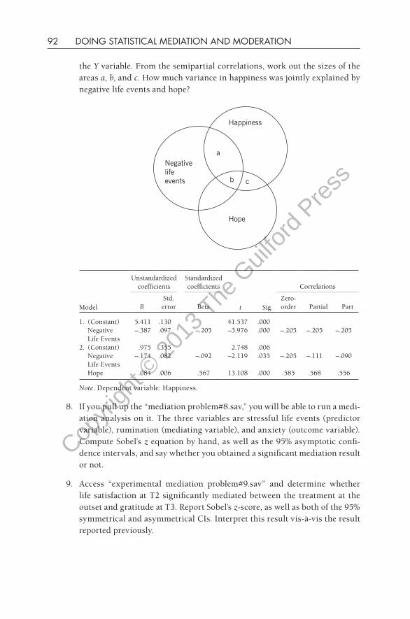
When one is interested in examining the ability of two predictor variables to predict an outcome (as in the case of mediation), one needs to be concerned about the potential overlap between the two predictors. In commonsense language, if we want to know how positive life events and gratitude predict happiness uniquely, then we need to consider how positive life events and gratitude are correlated. If they are significantly correlated (which will necessarily be the case in mediation), then there is a part of each that uniquely predicts happiness and a part in common with the other predictor that predicts happiness. Looking at Figure 3.18, the reader can discern that area b reflects the shared variance of positive life events and gratitude that also predicts happiness, whereas area a is the unique variance in happiness predicted by positive life events, and area c is the unique variance in happiness predicted by gratitude.
Tabachnick and Fidell (2001) present a nice exposition of these issues in their book (see also Cohen, Cohen, West, & Aiken, 2003). Tabachnick and Fidell examined the issue of two X variables predicting a single Y variable, which is exactly the case that we are considering here. They noted that “The total relationship of the IV with the DV and the correlations of the IVs with each other are given in the correlation matrix. The unique contribution of an IV to predicting a DV is generally assessed by either partial or semipartial correlation” (p. 139). (Note: The term semipartial correlation is considered to
a
b
d
Positive life events
Gratitude
Happiness
c
fIgURE 3.18. Shared and unique variance in mediation: the role of semipartial correlations.
be equivalent to the term part correlation, and statisticians and researchers use these terms interchangeably.) So it looks as though it would be useful to understand what semipartial correlations involve.
If I run a hierarchical regression in which happiness is the DV, positive life events is the first IV, and gratitude is the second IV, I obtain useful information about the ability of these two IVs to predict the DV. Specifically, I find that positive life events alone (in the first step) yields an R2 value of .115. This tells me that positive life events accounts for 11.5% of the variance in happiness by itself. The areas a and b together in the figure would represent 11.5% of the variance in happiness. Let us consider the second step: I find that the second IV gives us an R2 change value of .219. This means that area c in the figure represents 21.9% of the variance in happiness that gratitude explains above and beyond positive life events. In other words, gratitude uniquely explains 21.9% of happiness. But what about the ability of positive life events to uniquely explain happiness?
To determine this fact, we run the hierarchical regression with a reverse order of IV entry: gratitude first and positive life events second (see Table 3.19). This regression tells me that 30.2% of the variance in happiness is explained by gratitude in the first step (areas b and c), and in the second step positive life events uniquely predicts only 3.2% of the variance in happiness (area a). We now know the sizes of a (3.2%) and c (21.9%), and we can now mathematically determine the size of b by subtracting these two values from the total R2
(33.4%). After doing this computation, we obtain a value of 8.3% for area b. That is well and good, but how does this tell us anything useful about
semipartial correlations? This discussion is germane because SPSS and other statistics programs derive R2 values from squaring semipartial correlations. The R2 values tell the researcher about amounts of variance in the DV explained by the IVs, so this knowledge is helpful in determining the relative sizes of the direct and indirect effects in mediation. How does one obtain semipartial correlations, and what do they mean? Let us take a closer look at our data.
TABLE 3.19. derivation of the Amount of Shared Variance between the Two Predictor Variables (Area b)
I now return to the first step of the regression reported at the beginning of this chapter: Happiness is the DV and positive life events is the IV. I ask SPSS under STATISTICS for “part and partial correlations.” This option allows me to see these estimates in the output. (As noted earlier, terminology about semipartials is somewhat confusing, so it is important to know that SPSS uses “part” for what other writers refer to as “semipartial.”) Table 3.20 is what I obtained.
The partial and part (semipartial) correlations in the second step are illustrative in our current discussion. The partial correlation is the value we get when we hold constant some third variable from two other variables. Thus positive life events is correlated .214 with happiness, holding gratitude constant; and gratitude is correlated .498 with happiness, holding positive life events constant. However, our emphasis at this juncture is on the part (semipartial) correlation, and we can see that the part correlation for positive life events decreases from .338 on the first step to .179 on the second step. If we square these values, we see that positive life events goes from explaining 11.5% of the variance (area a + b) in happiness to 3.2% (area a) of the variance. Gratitude, entered at step 2, yields a part correlation of .468, and that value squared tells us that it uniquely explains 21.9% of the variance in happiness (area c). The remaining portion of variance explained in happiness by the two IVs, 8.3%, refers to area b, that portion explained jointly by the two IVs. We know that the total variance explained is .334, so removing .032 and .219 from the total yields .083. Thus positive life events and gratitude jointly explain about 8% of a person’s happiness.
TABLE 3.20. Statistical Output displaying Part (Semipartial) Correlations in a Hierarchical Regression
TABLE 3.21. Use of Part (Semipartial) Correlations in determining R2 Estimates of the Size of the Indirect Effect
Areas Part correlations Variances R2 estimates
a + b .338 .114 Total effect
a .179 .032 Direct effect
c .468 .219
b .083 Indirect effect
What is important to learn from this? The semipartial correlations provide another way to derive the R2 values necessary for computing the amounts of variance depicted in Figure 3.18. And by extension, they allow us to compute the R2 size of the indirect effect (see Table 3.21).
STATISTICAL ASSUMPTIONS
Now let us take up the issue of whether your data are appropriate for the linear regression analyses specified herein. One should not launch into these analyses without first determining whether one’s dataset satisfies a number of preconditions.
Power
Is your sample sufficiently large to give you enough statistical power to find a result of a reasonable size? To answer this question, according to Cohen (1992), four interrelated variables must be determined simultaneously: (1) the significance criterion (i.e., the alpha, usually set at .05 or .01); (2) sample size; (3) effect size; and (4) power level (usually set at 0.80). Using Cohen’s tables, one can determine a reasonable range for one’s sample size given values for the other three dimensions. For example, if I were to compute a linear regression for a mediational analysis—I’m trying to be relevant here—I would have two independent variables (the IV and the MedV), I would choose an alpha level of .05, I would assume a power level of 0.80, and I would assume that I would be looking for a medium effect size (based on previous analyses with the same variables). Looking through the table provided by Cohen, I would find that a sample of 67 should be sufficient. However, note that if I were seeking to obtain information for a small effect size, the sample size would swell to 481. Consequently, it makes a huge difference what types
of assumptions one makes for these analyses. In addition to Cohen’s tables in his article (1992) and his book (1988), there are other books that discuss this important issue (e.g., Kraemer & Thiemann, 1987), as well as online applets (e.g., G*Power, 2011; http://www.psycho.uni-duesseldorf.de/aap/projects/ gpower/). I would also recommend that interested readers examine two key articles written specifically about power in mediation analyses: MacKinnon et al. (2002) and Fritz and MacKinnon (2007). The essential conclusion of these latter investigations into various ways to compute mediation is that most studies of this type are underpowered (i.e., the sample is too small). In general, I recommend that researchers use samples that are somewhat larger than the “minimum number required” by these sources to give themselves some protection against this criticism.
distributions of Mediator and Outcome Variables
Tabachnick and Fidell (2001) have written a good chapter on “preparing one’s data,” and they argue that researchers need to examine their data to determine whether the variables adequately display normal distributions. The key issues are whether the distributions are skewed (i.e., the bulk of the scores are “smushed” against the left side or the right side of the scale) and whether they are kurtotic (i.e., the shape of the “hill” of scores is too flat or too peaked). They provide several equations that can be used to determine skewness and kurtosis, as well as a number of suggested transformations that can be used to normalize non-normal distributions. Severely skewed or kurtotic data can yield biased estimates when one performs statistical operations; that is, regression analyses for mediation or moderation might be “inefficient” or provide erroneous results. Word to the wise: Check your data to see whether they conform to basically normal distributions, and correct them if they do not.
Bivariate Assumptions
Even if you have verified that individual variables exhibit characteristics of a normal distribution, you are not necessarily out of the woods yet. Statisticians have identified a number of problems that can occur when one uses these variables in correlation or regression analyses. I briefly mention two issues of which a researcher should be aware: (1) Is there a linear relationship between the IV and DV? and (2) Are there normally distributed errors? When one computes a linear regression one is testing for a linear relationship, a fact that is sometimes lost on the beginning researcher. In practice, nonlinear
relationships are infrequently investigated. Examples of nonlinear relationships are quadratic (U-shaped) or cubic (S-shaped) patterns, and these can be probed by including additional terms in the basic regression equation (x2
and x3, respectively). See the section on quadratic moderation in Chapter 6 for more information. I believe that researchers should more often investigate whether nonlinear relationships between predictors and outcomes occur in their data, and this can be done by inspecting the pattern of residual versus predicted values (one should see a symmetrical pattern, not a bowed pattern).
The other issue mentioned concerns the distribution of residual errors. Just as with distributions of individual variables, there can also be outliers in the scatterplot of X-by-Y values of a correlation/regression. These outliers, if sufficiently extreme, have the power to significantly distort or bias obtained estimates, and we can identify them because they yield non-normal distributions of residual errors. In particular, if we obtain a normal probability plot of the residuals, we should see a normal distribution of residuals; but if the pattern is bow-shaped or s-shaped, then we may have a problem. These issues typically arise when the base distributions of individual variables are problematic and/or the relationship between them is not solely linear. So the way forward is simple: Make sure that the distributions of your individual variables are reasonably normal, and make sure that the relationships between predictor(s) and the outcome are principally linear.
SUMMARy
We have covered a lot of ground in this chapter. I have related how to compute the regressions necessary to test mediation (using the Baron and Kenny approach); I have laid out a number of examples; I have identified the potential problem of suppressor variables; and I have given the reader considerable information about the mathematical and statistical underpinnings of these regressions. Hopefully this chapter gives you a clear path forward in terms of accurately performing these analyses and drawing valid conclusions from the findings.
fURTHER REAdINg
I would suggest that the key readings to extend your understanding and knowledge in basic mediation analytical techniques would be the following:
Baron, R. M., & Kenny, D. A. (1986). The moderator–mediator variable distinction in social psychological research: Conceptual, strategic, and statistical considerations. Journal of Personality and Social Psychology, 51, 1173–1182.
Holmbeck, G. N. (1997). Toward terminological, conceptual, and statistical clarity in the study of mediators and moderators: Examples from the child-clinical and pediatric psychology literatures. Journal of Consulting and Clinical Psychology, 65, 599–610.
MacKinnon, D. P. (2008). Introduction to statistical mediation analysis. Mahwah, NJ: Erlbaum.
MacKinnon, D. P., Fairchild, A. J., & Fritz, M. S. (2007). Mediation analysis. Annual Review of Psychology, 58, 593–614.
IN-CHAPTER ExERCISES
1. Significant mediation. If you would like practice in computing basic linear regression-based mediation analyses, go to http://crmda.ku.edu/guilford/ jose and download the dataset named “mediation example.sav.” This is the first dataset described in this chapter; it concerns three variables from the positive psychology subdiscipline, namely positive life events, gratitude, and happiness.
2. Experimental mediation. The chief difference with experimental data, usually, is that the IV is a dichotomous categorical variable, and one can logically place variables into the three slots on the basis of temporal occurrence.
3. Null mediation. Again, if you would like to practice conducting mediation, and in this case obtain null mediation (how exciting!), you can download the dataset named “null mediation example.sav” and hopefully obtain the same results that I detailed herein.
4. Mediation with a suppressor variable. If you download the dataset named “suppressor mediation example.sav,” you can have a go at duplicating the results obtained in this chapter.
AddITIONAL ExERCISES
1. Examine the following correlation matrix. Obviously, gender is a dichotomous categorical variable (1 = females; 0 = males), and the remainder are continuous variables. These variables were all measured at a single point of measurement (i.e., concurrent), and no variable was manipulated in an experimental fashion. How many and which specific possible mediational
relationships could be tested with this particular group of variables? Assume that a significant relationship must be noted between variables for them to be included in these models. (Bonus point: If we loosen the assumptions to allow for a nonsignificant IV-to-DV relationship, do any more mediation analyses become possible?)
2. What can we conclude from this result? In this case, Sobel’s z = 2.02, p < .05, beta weights are reported, and coefficients in parentheses were taken from the X, M predicting Y regression.
Intelligence Problem solving
Accuracy of long-term memory
0.467 0.378 (0.538)
(0.343)
0.286
3. Given the standardized regression coefficients depicted in the following figure, identify the values for (a) the direct effect, (b) the indirect effect, (c) the total effect, and (d) the ratio of the indirect/total for standardized regression coefficients.
6. Which area (or areas) in the following figure refer to (a) the total effect, (b) the direct effect, and (c) the indirect effect? Bonus point: What does area d refer to?
MedV
7. In the following mediation example, I have set negative life events (stress) to be the X variable, hope the potential mediating variable, and happiness
the Y variable. From the semipartial correlations, work out the sizes of the areas a, b, and c. How much variance in happiness was jointly explained by negative life events and hope?
8. If you pull up the “mediation problem#8.sav,” you will be able to run a mediation analysis on it. The three variables are stressful life events (predictor variable), rumination (mediating variable), and anxiety (outcome variable). Compute Sobel’s z equation by hand, as well as the 95% asymptotic confidence intervals, and say whether you obtained a significant mediation result or not.
9. Access “experimental mediation problem#9.sav” and determine whether life satisfaction at T2 significantly mediated between the treatment at the outset and gratitude at T3. Report Sobel’s z-score, as well as both of the 95% symmetrical and asymmetrical CIs. Interpret this result vis-à-vis the result reported previously.