JML-CT-fl-21

MASTBf

SAMPLI PIOILBf CALCULATIONS IBLA3XD TO

TWO-PHASE fLCW TMMSIBItS » A ^

by

Tons V . Shin and Arn* H. Wicdcraann

• : • • , ; • • • ; / • * <

• - : : : ' - • ' • . » » ' : • : - - - • ; -

S. Di^iiar CMtxact 1

' • " • • • " • • ' • - • ; • • • . : • .

Mt Of1-31-11

Of THIS 20CUMMT IS UCUt

ANL-CT-81-21Oiatribution Category:Light Water Reactor Technology(UC-78)

ARGONNE NATIONAL LABORATORY9700 South Cass Avenue

Argonne, Illinois 60439

SAMPLE PROBLEM CALCULATIONS RELATED TOTWO-PHASE FLOW TRANSIENTS IN A

RELIEF-PIPING NETWORK

by

Yong W. Shin and Arne H. Wiedermann*

Components Technology Division

March 1981

•Consultant; affiliated with ATResearch Associates, Inc.,Glen Ellyn, Illinois

CJ!:";::T;GI! M r--:;s •i ure;;-; is L^

TABLE OF CONTENTS

Page

ABSTRACT vii

I. INTRODUCTION 1

II. NEW BOUNDARY CONDITIONS IMPLEMENTED IN STAC CODE 2

A. Specified-Mass-Flow-Rate Boundary 2

B. Material Interface as Moving Boundary 3

C. New Set of Interpolation Formulas 4

1. Interpolation Formulas for Characteristics at 5Interface Location

2. Other Special Interpolation Formulas 6

III. DESCRIPTION OF SAMPLE PROBLEMS 8

IV. ANALYTICAL SOLUTIONS 9

A. Sample Problem No. 1 9

1. Contoured-Inlet-Geometry Case 9

a. Similarity Solution for Rarefaction Fan 10b. Comparison of Analytical Solutions with Code

Calculation 11

2. Abrupt-Inlet Geometry Case 12

B. Sample Problem No. 2 13

V. CODE CALCULATIONS AND COMPARISON WITH ANALYTICAL SOLUTIONS 15

A. Sample Problem No. 1 15B. Sample Problem No. 2 15

VI. COMPUTATIONAL DIFFICULTY AT MATERIAL INTERFACE WITH LARGE

IMPEDANCE GRADIENT 17

VII. SUMMARY AND CONCLUSIONS 19

ACKNOWLEDGMENTS 20

REFERENCES 20

iii

LIST OF ILLUSTRATIONS

No. Title Page

1 Specified-Mass-Flow Boundary 26

2 Solution Methodology for Specified-Mass-Flow-Rate Boundary 26

3 Material Interface in an Interior Computing Cell 26

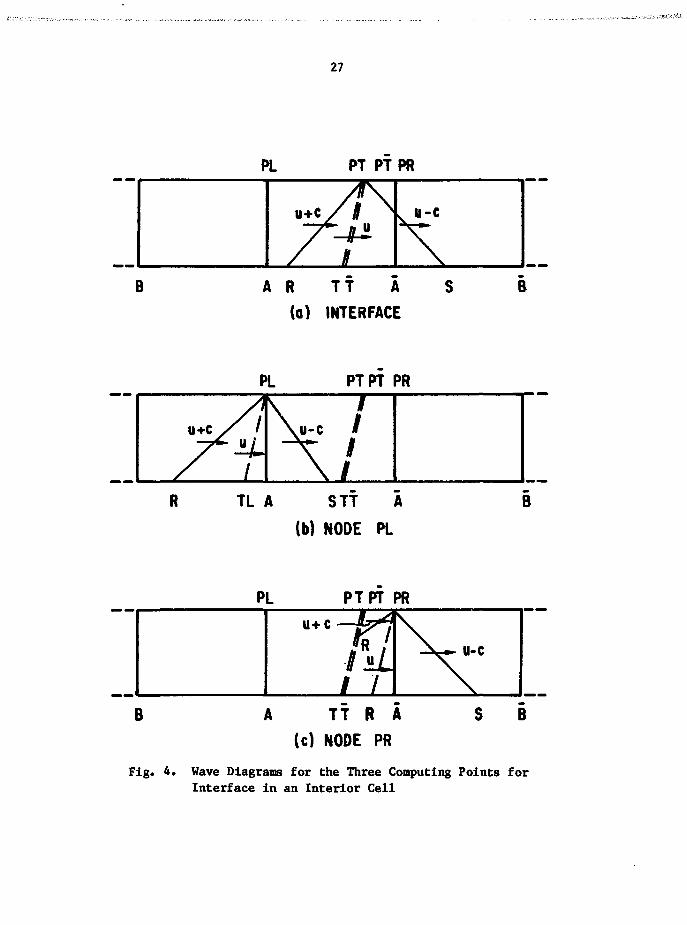
4 Wave Diagrams for the Three Computing Points for Interface

in an Interior Cell 27

5 Solution Methodology for the Interface 28

6 Wave Diagrams for the Interface in the Boundary Cell 28

7 Wave Diagram for a Typical Computing Node 28

8 Characteristics Configurations for the Material Interface 29

9 Characteristics Configurations for Adjacent Node PL 30

10 Characteristics Configurations for Adjacent Node PR 31

11 Sample Problem No. 1 32

12 Solution for the Shocked State (Well-Contoured Inlet) 33

13 Wave Diagram (Well-Contoured Inlet Case) 33

14 Applicable Characteristics and Compatibility Condition forExpansion Fan (Quiescent Initial State) 34

15 Applicable Characteristics and Compatibility Condition forExpansion Fan (Shocked Initial State) 34

16 Shock Wave and Interface Locations 35

17 Pressure and Velocity Profiles at t - 3.85 ms 36

18 Temperature and Sonic Speed Profiles t - 3.85 ms 36

19 Pressure and Velocity Profiles at t * 9.66 ms 37

20 Temperature and Sonic Speed Profiles at t - 9.66 ms 37

21 Pressure and Velocity Profiles at t * 25 ms 38

22 Pressure Histories 38

23 Pressure Histories 39

24 Forces on Segment A-C (F - F ) 39x y

25 Pressure Hisotry at Location B(x * 2.5 ft) 40

26 Velocity History at Location B(x - 2.5 ft) 40

27 Pressure History at Location D(x - 25 ft) 41

28 Velocity History at Location D(x - 25 ft) 41

29 Pressure and Velocity Profiles at t - 9.7 ms 42

30 Temperature and Sonic Speed Profiles at t » 9.7 ms 42

iv

LIST OF ILLUSTRATIONS (Cont'd)

No. Title Page

31 Force on Segment on A-C (F ) 43

32 Solution for the Shocked State (Abrupt Inlet Case) 43

33 Wave Diagram (Abrupt Inlet Case) 44

34 Similarity Solution - Pressure Result 44

35 Similarity Solution - Particle Velocity Result 45

36 Similarity Solution - Temperature Result 45

37 Wave Diagram for Sample Problem No. 2 46

38 p-u Diagram for Sample Problem No. 2 (Ap = 1.63 psi;

Au = 9.14 fps) 46

39 Shock Wave and Interface Locations 47

40 Pressure and Velocity Profiles at t = 0.69 ms 48

41 Temperature and Sonic Speed Profiles at t = 9.69 ms 48

42 Pressure History at x = 2.5 ft 49

43 Pressure History at x = 25 ft 49

44 Force on Segment A-C 50

45 Pressure and Particle Velocity Profiles at t = 10.4 ms 50

46 Pressure and Particle Velocity Profiles at t = 30.4 ms 51

47 Pressure History at x = 2.5 ft 51

48 Particle Velocity History at x * 25 ft 52

49 Force of Segment A-C 5250 Characteristics Configuration with Disturbance Front at the

Interface 53

51 p-u Diagram for Simulant Steam Compared to Nitrogen Gas 54

52 Wave Diagram for the Simulant Superheated Steam 54

53 Pressure Histories Comparison: Steam-N_ vs Simulated System 55

54 Comparison of Forces on Segment A-C: Steam-N_ vs SimulatedSystem 55

LIST OF TABLES

No. Title Page

1 Interpolation Formulas for the Characteristics Configurationsof Material Interface (Refer to Fig. 8 for specific configur-ations) 21

2 Interpolation Formulas for the Characteristics Configurationsof Node PL (Refer to Fig. 9 for specific configurations) 22

3 Interpolation Formulas for the Characteristics Configurationsof Node PR (Refer to Fig. 10 for specific configurations) 23

4 Comparison of Properties of Simulant Superheated Steam andNitrogen Gas 25

vi

SAMPLE PROBLEM CALCULATIONS RELATED TOTWO-PHASE FLOW TRANSIENTS IN A PWR

RELIEF PIPING NETWORK

Yong W. Shin

Conponents Technology DivisionArgonne National Laboratory

9700 S. Cass AvenueArgonne, Illinois 60439

Arne H. Wiedermann

ATResearch Associates, Inc.94 Main Street

Glen Ellyn, Illinois 60137

ABSTRACT

Two sample problems related with the fast transients of water/steamflow in the relief line of a PWR pressurizer were calculated with anetwork-flow analysis computer code STAC (System Transient-Flow An-alysis Code). The sample problems were supplied by EPRI and are de-signed to test computer codes or computational methods to determinewhether they have the basic capability to handle the important flowfeatures present in a typical relief line of a PWB pressurizer. Itwas found necessary to implement into the STAC code a number of ad-ditional boundary conditions in order to calculate the sample prob-lems. This includes the dynamics of the fluid interface that istreated as a -moving boundary. This report describes the methodol-ogies adopted for handling the newly implemented boundary conditionsand the computational results of the two sample problems. In orderto demonstrate the accuracies achieved in the STAC code results, an-alytical solutions are also obtained and used as a basis for compar-ison.

vii

I. INTRODUCTION

ANL participated in an EPRI program in which a number of computer codes

were used to calculate the sample problems that are designed to test the var-

ious codes in their ability to predict the two-phase flow transients in the

relief piping network of a PWR. The computer code used for ANL participation

is the STAC (System Jransient-Flow Analysis Code) code that has been developed

at ANL under a code development program for analysis of large-scale sodium-

water reactions. The STAC code forms a module of the sodium-water reaction

analysis code SWAAM-I (Sodium-Water Advanced Analysis Method - Version I) [1].

The STAC code is a homogeneous two-phase flow-transients analysis code for

piping networks and is based on the finite-difference technique using the ar-

tificial viscosity concept for solution of interior flow field, but on the

method of characteristics to treat the boundary conditions and junction con-

ditions. During the STAC code development, it was recognized that the phase

change, or more specifically the drastic change in the impedance (pc) frequent-

ly existing at the boundary, required a special numerical treatment in order

to successfully carry out the computation. Hence, a new technique is intro-

duced in the STAC code to overcome the difficulty. The technique is a semi-

analytical procedure based on the method of characteristics using a subsize

time-step [2]. It has been proven that very accurate results can be obtained

with the boundary technique.

In the beginning of this work of calculating the EPRI sample problems, a

number of code modifications were necessary in order to carry out the work. A

number of additional boundary condition options had to be implemented in the

code, and that included the material interface boundary treated as a moving

boundary. While the numerical technique implemented in the STAC code is accu-

rate and stable, it requires an extensive amount of coding work. As a result

of this inherent nature of the STAC code, the coding work involved in this

present study was rather major. Nevertheless, the required coding work was

completed and the sample problems calculated. In addition to the code calcu-

lations, analytical solutions were also obtained for reduced problems where

certain second-order effects were neglected. The analytical solutions were

used as a basis of comparison to demonstrate the accuracy of the numerical re-

sults for the sample problems.

II. NEW BOUNDARY CONDITIONS IMPLEMENTED IN STAC CODE

A. Specified Mass-Flow-Rate Boundary

It is often desirable to consider a boundary condition in which the mass-

flow rate is specified, as in this present study. This boundary condition is

especially important in analysis of test results where the mass flow rate is

measured directly or indirectly and would like to maintain that condition at

some point in the system.

Following the basic boundary-condition methodology [2], the entropy at

the boundary, at the advanced time (t + At), s , is first estimated by the

upstream condition following the material characteristic equation (Eq. 10 of

Ref. 2). If the upstream is a reservoir with a large inventory of mass, the

entropy is set to the entropy for the reservoir. Once the entropy is deter-

mined, the remaining task is to compute the remaining two variables of the

three-variable system on hand, namely, the pressure (p) and particle velocity

(u). These are computed in the p - u plane by a substep procedure as described

schematically in Fig. 2. Figure 1 shows the physical configuration and the

wave diagram for the subject boundary condition. Figure 2 shows the mass line

and sonic line for a constant entropy s = s . The compatibility equations for

the u - c characteristics are also drawn in Fig. 2 for the neighboring states

S. When the neighboring state S is at a high pressure, the solution state for

the boundary is subsonic; i.e. P, in Fig. 2. But for a low enough pressure for

state S, the solution state can be supersonic, namely, state P1. The super-

sonic state at the pipe inlet by a specified mass flow rate is only possible

if the inlet section of the pipe is well contoured to permit such flow accel-

eration. Normally, this condition does not exist in the piping system, and

hence it is assumed that the pipe area changes abruptly. The flow at the in-

let then should be limited by choking. The solution state therefore is the

state P for all sufficiently low pressures of the neighboring state S. Note

that the compatibility equations are drawn schematically as straight lines in

Fig. 2, but in the linear scale of p and u, they can be severely curved due to

the large change in the impedance (pc) between one time step (At). This is

the reason the compatibility equations have to be numerically integrated by

substeps (At/N) in order to locate the accurate solution state. This is not

necessary when the impedance does not change much during the step calculation.

The usual water-hammer transient is an example of a nearly constant impedance

[3-5].

B. Material Interface as Moving Boundary

Often the piping system involves more than one fluid, and it is desirable

to follow the dynamics of the material interface without allowing mixing of

the two fluids. For the subject sample problems, for example, the piping had

nitrogen gas in the line, and steam or water is to be introduced at one end

of the piping to initiate the transient. Often when the interface tracking

capability does not exist in a code, an attempt is made to approximate the

two-fluid system by a single fluid at certain adjusted initial conditions.

But this practice is not always very successful, as can be seen from the dis-

cussion later in this report. Also shown in this study is that, even for a

single fluid system when the large change in fluid property is simulated by

an interface, namely the water seal/steam situation in the PWR relief piping,

very accurate results can be obtained.

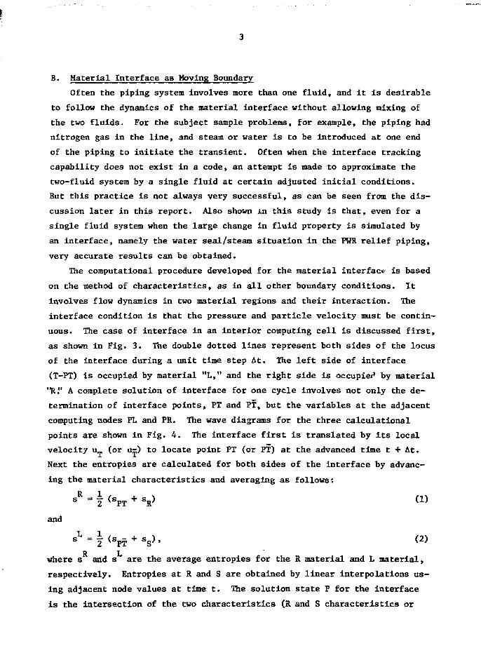
The computational procedure developed for the material interface is based

on the method of characteristics, as in all other boundary conditions. It

involves flow dynamics in two material regions and their interaction. The

interface condition is that the pressure and particle velocity must be contin-

uous. The case of interface in an interior computing cell is discussed first,

as shown in Fig. 3. The double dotted lines represent both sides of the locus

of the interface during a unit time step At. The left side of interface

(T-PT) is occupied by material "L," and the right side is occupier1 by material

"R." A complete solution of interface for one cycle involves not only the de-

termination of interface points, PT and PT, but the variables at the adjacent

computing nodes PL and PR. The wave diagrams for the three calculational

points are shown in Fig. 4. The interface first is translated by its local

velocity u (or u=) to locate point PT (or PT) at the advanced time t + At.

Next the entropies are calculated for both sides of the interface by advanc-

ing the material characteristics and averaging as follows:

sR) (1)

and

s L = | (sp- + ss) , (2)

R Lwhere s and s are the average entropies for the R material and L material,

respectively. Entropies at R and S are obtained by linear interpolations us-

ing adjacent node values at time t. The solution state P for the interface

is the intersection of the two characteristics (R and S characteristics or

rthe compatibility equations) for the two fluid regions at the respective en-

R L

tropies, s = s for the u + c and s = s for the u - c as described in Fig.5.

Again the characteristics are represented schematically by straight lines, but

can be severely curved. The same procedure applies to the adjacent nodes,

node PL and PR, except that the two characteristics are for the same entropy,L Rs or s , since both characteristics lie in the same fluid region. In fact,the representative entropies are averaged as follows:

s = j (sR + s p L + sg) for node PL (3)

and

j (sR + s p R + sg) for node PR, (4)

respectively. Note that the neighboring states R and S can lie on the locus

of interface, such as the point R in Fig. 4c.

The case when the interface is located in the boundary cell is treated

essentially the same way. Figure 6 shows the wave diagrams for the interface

in the inlet and outlet cells. Here, too, the interface is first advanced

and then the adjacent node. Since the interface is done before the boundary

node, when the characteristic hits the boundary no interpolation can be made

along the time line (x = const). In this case an approximation is made as

shown in Fig. 6a, where the neighboring state R is assumed to collapse on

point A. Besides this exception, the procedure is identical to the case of

the interface in the interior cell. The adjacent nodes PR and PL are computed

exactly the same way as discussed above for the interior cell. The solution

methodologies for the boundary nodes, however, are slightly modified. The

neighboring states, state R or S, are now obtained by interpolation along the

interface path or the initial time line, but limited to the appropriate side

of the interface.

C. New Set of Interpolation Formulas

The characteristics applied to a computing point of a finite-difference

system requires evaluation of neighboring states that fall between computing

nodes. As shown in Fig. 7, computation of node P requires determination of

the neighboring states R, T, and S. A linear distribution of variables is

assumed between the nodes. Moreover, the slope of characteristics is approx-

imated by that of the initial plane, namely, at R, T, or S. Under these as-

sumptions, the following can be written for point R, for example:

(c + u ) R = f • (c + u ) c + (1 - f) • (c + u ) A , (5)

(c + u ) D At = f • Ax, (6)

and

f = RA/Ax. (7)

Solving for f by eliminating (u + c ) D results in the desired interpolation

formula for location of point R:

(c + u).f = - . (8)

Ax . , , . , . *"7— + (c + u) — (c + u ) n

Similarly the following formulas may be obtained for points T and S, respec-

tively:

(U)A— (9)Ax . , . - .

A£ + (u)A - (u)cand

(c - u)f = A

f£ + ( c - u ) A - ( c - u ) B

These formulas apply to the neighboring states falling between the spec-

ified computing nodes at the initial plane and are used to evaluate the states

at those points. For the interface procedures discussed above, however, the

neighboring-state points do not always fall between computing nodes and spe-

cial interpolation formulas must be developed.

1. Interpolation Formulas for Characteristics at Interface Location

The u ± c characteristics at the interface location are drawn in

Fig. 8. The u + c characteristic lies on the left of the particle path; the

u - c characteristics lies on the right. As discussed above, the particle

path is advanced first, and hence DIXP of Fig. 8 is known, and the interpola-

tion formulas are applied to locate the neighboring states R and S. There are

two reasons why special formulas must be developed that differ from the stan-

dard formulas applicable to regular nodes (Eqs. 8-10). The first reason is

that the interface lies between the nodes so that the distances DIXP and DIX

enter in the formula. The other reason is that the interpolation to be made

can be between the node point and the interface location, instead of between

nodes only as in the standard case. Figure 8 shows the two possible cases for

each of the two characteristics u t c. For the case 1 configuration of Fig.

8, for example, the following two relations can be written:

(c + u ) R = f • (c + u ) T + (1 - f) • (c + u ) A

and

(c + u)_ • At = - f • DIX + DIXP,K

(12)

where

AR/DIX,

and from these; relations the following interpolation can be obtained:

/ __ -, DIXP

£ (c + U)

A - sr(c - (C

(13)

Similar formulas may be obtained, and the results are given in Table 1 for the

four configurations shown in Fig. 8.

2. Other Special Interpolation Formulas

Calculation of the interrace by the method of characteristics, namely,

points PT and PT of Fig. 3, requires similar calculations for the two adjacent

nodes PL and PR. Again for these calculations, the characteristics may fall

between points that are not always the grid points that are fixed. 3"or compu-

tation of PL, for example, the u - c characteristic may fall between points

A and T, and a special formula is needed. Likewise u + c characteristic for

PR may fall between f and A. In addition, the characteristics can fall on the

interface line, namely, the line connecting T and PT or the line connecting T

and PT.

Nine different configurations are identified for PL-node calculations

for the three characteristics, u + c, u - c, and u, as shown in Fig. 9. The

procedure for determining the interpolation formulas is similar to that used

for the interface and hence is not repeated here, but the formulas are listed

in Table 2. There are two possible configurations, however, as shown in Figs.

9e and 9i where the u + c characteristics intersect the interface and, hence,

require interpolations not only along distance (x), but also along time (t).

The interpolation formula for configuration case 5 is derived below. The

(u + c) characteristic crosses the interface and, hence, extends to the other

side of the material region. In determining the state R, a continuity is

assumed of the right-hand-side-material states, even into the left of the

interface, so that an extrapolation is made for state ft. Then the following

two relations can be written:

(c + u)ft - (c + u ) £ + f . [(c + u ) ^ - (c + u)-] (14)

and

(c + u)z • At = f • DIX - Ax (15)

From these equations the following formula can be written:

£ =

Since the neighboring state in this configuration is the state R located on

the interface, linear interpolations are applied along the interface and the

c + u characteristic. Since both lines are now defined, the intersection of

the two lines are solved, the interpolation formula defining g (see Fig. 9e)

can be obtained:

a = (f - 1) • DIXg (f - 1) • DIX + DIXP - Ax* K '

Similar formulas are obtained for Case i of Fig. 9 and are included in

Table 2.

Another nine configurations are shown in Fig. 10 for node PR, and

the corresponding formulas are derived and shown in Table 3. In essence the

procedure used in deriving the formulas for node PR is the same as that used

for node PL.

III. DESCRIPTION OF SAMPLE PROBLEMS

The sample problems considered here for STAC code calculation are the

blowdown transient from a large pressure vessel and through a connected pip-

ing. The other end of the piping is the low-pressure end exposed to the ambi-

ent at 14.7 psia pressure. The piping is filled initially with nitrogen gas

at room temperature and ambient pressure. Instead of specifying the valve

area, the mass flow rate m is given. The desired results of the calculation

are the pressure-time histories at points B and D of Fig. 11, and the forces

acting on che pipe segment AC (including the elbow).

A. Sample Problem No. 1

Sample problem no. 1 is described in Fig. 11. It consists of the blow-?

down of dry saturated steam at 2400 psia through the safety valve and the down-

stream piping, 9.564-in. ID and 25 ft long. The valve opening is replaced by

a specified mass flow rate m = 560,000 lbm/hr. The piping is filled with low-

pressure nitrogen gas, and hence, the initial transient involves the shock

waves generated at the valve (initial material interface location) and their

propagation and interaction in the pipe. The initial and boundary conditions

are defined, and the problem is ready for numerical solution by STAC code with

the code extensions as discussed above. The code models the pipe in between

the two boundaries, namely, the specified mass-flow-rate boundary and the out-

flow (or break-end) boundary.

B. Sample Problem No. 2

Sample problem no. 2 is identical to the sample problem no. 1 in geometric

configuration, but considers the flow of cold water instead of dry saturated

steam as in the sample problem no. 1. The water condition is at 100°F (0.9

psia saturation pressure); hence, the water is expected to remain as water

(i.e., no phase change). The water flow rate is 200 gpm. Aside from this

difference, the two sample problems are identical.

IV. ANALYTICAL SOLUTIONS

Seeking analytical solutions for the sample problems was an important

part of the task. The analytical solutions not only served as a basis for

comparison with the code results, but also helped in learning the physical

nature of the problems. The STAC code is based on a semianalytical approach

and is capable of producing very accurate results. The accuracies of the STAC

code results are demonstrated by direct comparisons of the results with ana-

lytical solutions as is discussed later in this report. The wave system

involved in the two sample problems were simple, and it was possible to obtain

analytical solutions when certain secondary effects were neglected. The ef-

fects of gravity and friction are neglected in the analytical solutions.

A. Sample Problem No. 1

Sudden opening of the valve develops a shock wave traveling down the pipe

followed by the material interface moving at the particle velocity. Depend-

ing on whether the pipe inlet geometry is well-contoured or sharp-edged, the

inlet rotate of flow can be locally either supersonic or choked. First, the

case of supersonic inlet condition is considered.

1. Contoured-Inlet-Geometry Case

The solution is obtained by a simultaneous solution of the constant

mass line (m = const) and the nitrogen Hugoniot in the p - u diagram at a con-

stant entropy, as shown in Fig. 12. The intersection of the two lines is the

state of the shocked region. The solution obtained is used in the wave dia-

gram shown in Fig. 13. There are three regions of constant state: the undis-

turbed nitrogen region at state S^ (14.7 psia and 70°F), the shocked nitrogen

region at state S-, and the expanded steam region S_. The interface separates

the two materials across which the interface conditions u.. = u« and P. = p_

are maintained. The solution is summarized below:

1

1u =

1

1

P2 =

U2 =

2770

1483

424.

1215

64.64

1408.4

.5 ft/s

.3 ft/s

8°F

ft/s

psia,

ft/s

297.6°F

(18)

10

A narrow fan rarefaction system develops at the end of the pipe,

since the particle velocity in region S.. is slightly less than the sonic speed

when the shock wave reflects from the outlet end. In the steam region, S_,

however, the state is supersonic, and hence, the rarefaction system blows out

of the pipe. The rarefaction system is shown in Fig. 13, and the flow remains

choked at the outflow end during the rarefaction.

a. Similarity Solution for Rarefaction Fan

Consider first an expansion fan at x « 0 propagating into a qui-

escent state of a gas region. The applicable characteristics are the c - u

characteristics and the compatibility condition for the c + u characteristic

as shown in Fig. 14. For an assumed ideal gas, the applicable equations can

be written as

| = c - u (19)

and

(20)

or in a dimensionless form

5 - X " • (21)

and

X + l L f A • - 1. (22)

where

c - F T • <23>o

X - f- . (24)o

• - f- (25)o

Eliminating 4> and x from Eqs. 21 and 22 results in the desired solutions for

X (or <J> after substitution) in terms of the similarity variable £ as follows:

(26)

11

and

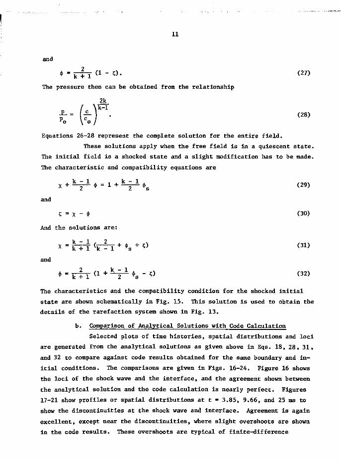
* -j^TT (1 " °- (27)

The pressure then can be obtained from the relationship

And the solutions are:

(28)

Equations 26-28 represent the complete solution for the entire field.

These solutions apply when the free field is in a quiescent state.

The initial field is a shocked state and a slight modification has to be made.

The characteristic and compatibility equations are

(29)

(30)

k + 1 vk - 1 ' *s • "' ( 3 1 )

and

O 1, 1

- C) (32)

The characteristics and the compatibility condition for the shocked initial

state are shown schematically in Fig. 15. This solution is used to obtain the

details of the rarefaction system shown in Fig. 13.

b. Comparison of Analytical Solutions with Code Calculation

Selected plots of time histories, spatial distributions and loci

are generated from the analytical solutions as given above in Eqs. 18, 28, 31,

and 32 to compare against code results obtained for the same boundary and in-

itial conditions. The comparisons are given in Figs. 16-24. Figure 16 shows

the loci of the shock wave and the interface, and the agreement shown between

the analytical solution and the code calculation is nearly perfect. Figures

17-21 show profiles or spatial distributions at t = 3.85, 9.66, and 25 ms to

show the discontinuities at the shock wave and interface. Agreement is again

excellent, except near the discontinuities, where slight overshoots are shown

in the code results. These overshoots are typical of finite-difference

12

techniques using artificial viscosity and results from the interior field

procedure that is based on the Lax-Wendroff scheme (see Ref. 2). The inter-

face discontinuities are well represented in the code results, and this indi-

cates the general capability of the semianalytical boundary technique imple-

mented in STAC code. The procedure used in the interface calculation is based

en the same general boundary procedure, and the accuracy shown in these fig-

ures near the interface is to be expected. Pressure-history plots are given

in Figs. 22 and 23. The history plot for point D (outlet end) shown in Fig.

22b shows the effect of the rarefaction system. Again the slight numerical

overshoots are evident. Finally, the fluid forces acting on the segment A-C

including the elbow are shown in Fig. 24. The longitudinal force F is iden-

tical to the lateral force F in the absence of gravity and friction as in the

case here.

It was of interest to see the effects of gravity and friction, although

they are considered second-order effects, at least for the early time trans-

ients, when most important wave effects take place. An additional code cal-

culation was therefore made for the same left-end boundary condition allowing

the supersonic inflow. The results are presented in Figs. 25-31. These re-

sults are similar to the results discussed above where the second-order ef-

fects of gravity and friction are neglected. Therefore no additional discus-

sion is necessary, except to note the effects of the gravity and friction.

Comparison of the plots with the corresponding ones for the simplified problem

(no gravity-no friction) indicates that the relaxation is longer with gravity

and friction than without. This is shown by the wavy nature of the plots, as

can be seen in Figs. 25 and 26. The secondary effects add long-wavelength os-

cillation to the solution.

2. Abrupt-Inlet-Geometry Case

Abrupt geometry is more common in piping systems than the contour-

ed geometry. The abrupt-geometry assumption was therefore adopted for STAC

code development. In the sample problems under investigation, the inlet of

the pipe (downstream section of the valve) may be closely modeled by an abrupt-

inlet geometry and the basic assumption is well justified. The difference be-

tween this inlet boundary condition and the contoured-inlet case is that the

flow chokes at the inlet with the expansion taking place in the pipe for the

case of the abrupt inlet while the inlet flow is supersonic in the contoured-

inlet case. This difference is clearly seen by comparison of Figs. 13 and 33.

13

First the shocked state is to be determined. As shown in the cen-

tered rarefaction wave system developed at the pipe inlet as shown in Fig. 33,

the sonic condition at the inlet expands further into a supersonic state. The

choked inlet state S. is the intersection of the constant mass-flow line and

sonic line as shown in Fig. 32. Further expansion from the inlet choked state

follows C characteristic in the solution plane (the compatibility condition

for u + c characteristic). The shocked state or the solution state is then

the simultaneous solution of the C characteristic for steam and the nitrogen

Hugoniot. This means that the solution state is the intersection of the C

characteristic and nitrogen Hugonoit in the p - u diagram Fig. 32. The pres-

sure and velocity are continuous across the material interface. The solution

is as follows:

Px = P2 = 63.97 psia

u± = u 2 = 1396.5 ft/s

U = 2259 ft/s

C;L = 1217.7 ft/s ^ (32)

Tx = 296.9°F

c2 = 1479.8 ft/s

T2 = 420.6°F

The solution is plotted in terms of the similarity variable x/t as shown in

Figs. 34-36. The inlet expansion fan region is solved by computer. The ex-

pansion waves expressed by

- = u - c (33)

correspond to points on the C characteristic of Fig. 32. Therefore a com-

plete solution is obtained for the rarefaction wave system at the inlet. The

small rarefaction system at the outflow end is also solved. The procedure

used here is similar to the one discussed in Sec. 1 above. The complete ana-

lytical solution is given later in the report where the code result is dis-

cussed and compared with the analytical result.

B. Sample Problem No. 2

Because of the low flow rate, the disturbance level is very low. For this

low-disturbance system, the water-hammer waves in the water region may be

14

neglected, and the interface may simply be treated as a constant-velocity

boundary like a piston. For this simple system, the wave system is simply a

reverberation of waves between the piston at one end and the constant pressure

boundary at the other. The solution obtained is shown in the wave diagram of

Fig. 37 and the p - u diagram of Fig. 38. It is essentially an acoustic sys-

tem with pressure disturbance Ap = 0.163 psi and corresponding velocity dis-

turbance Au = 9.14 fps.

15

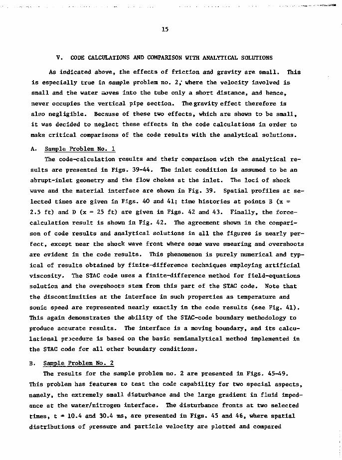
V. CODE CALCULATIONS AND COMPARISON WITH ANALYTICAL SOLUTIONS

As indicated above, the effects of friction and gravity are small. This

is especially true in sample problem no. 2,' where the velocity involved is

small and the water moves into the tube only a short distance, and hence,

never occupies the vertical pipe section. The gravity effect therefore is

also negligible. Because of these two effects, which are shown to be small,

it was decided to neglect these effects in the code calculations in order to

make critical comparisons of the code results with the analytical solutions.

A. Sample Problem No. 1

The code-calculation results and their comparison with the analytical re-

sults are presented in Figs. 39-44. The inlet condition is assumed to be an

abrupt-inlet geometry and the flow chokes at the inlet. The loci of shock

wave and the material interface are shown in Fig. 39. Spatial profiles at se-

lected times are given in Figs. 40 and 41; time histories at points B (x =

2.5 ft) and D (x = 25 ft) are given in Figs. 42 and 43. Finally, the force-

calculation result is shown in Fig. 42. The agreement shown in the compari-

son of code results and analytical solutions in all the figures is nearly per-

fect, except near the shock wave front where some wave smearing and overshoots

are evident in the code results. This phenomenon is purely numerical and typ-

ical of results obtained by finite-difference techniques employing artificial

viscosity. The STAC code uses a finite-difference method for field-equations

solution and the overshoots stem from this part of the STAC code. Note that

the discontinuities at the interface in such properties as temperature and

sonic speed are represented nearly exactly in the code results (see Fig. 41).

This again demonstrates the ability of the STAC-code boundary methodology to

produce accurate results. The interface is a moving boundary, and its calcu-

lational procedure is based on the basic semianalytical method implemented in

the STAC code for all other boundary conditions.

B. Sample Problem No. 2

The results for the sample problem no. 2 are presented in Figs. 45-49.

This problem has features to test the code capability for two special aspects,

namely, the extremely small disturbance and the large gradient in fluid imped-

ance at the water/nitrogen interface. The disturbance fronts at two selected

times, t • 10.4 and 30.4 ms, are presented in Figs. 45 and 46, where spatial

distributions of pressure and particle velocity are plotted and compared

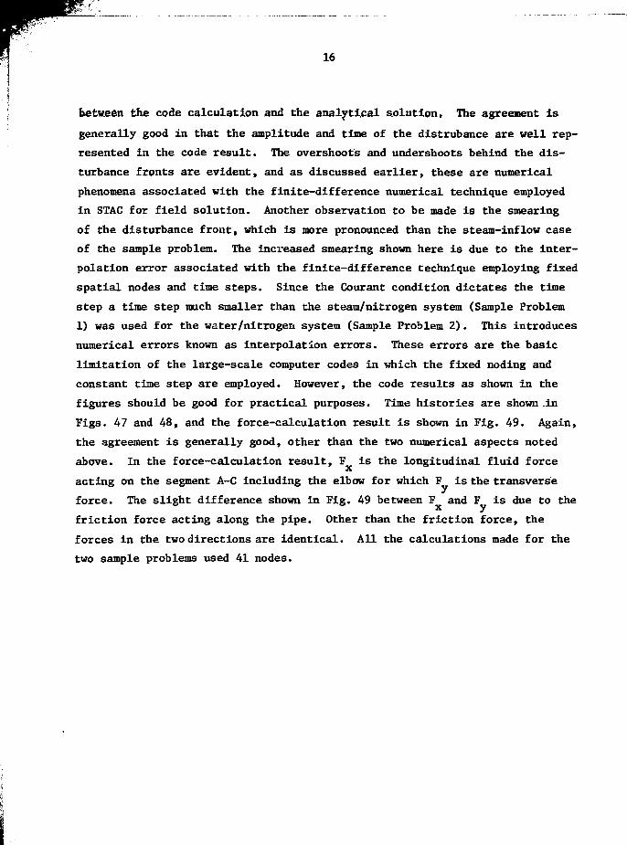
16

between the code calculation and the analytical solution. The agreement is

generally good in that the amplitude and time of the distrubance are well rep-

resented in the code result. The overshoots and undershoots behind the dis-

turbance fronts are evident, and as discussed earlier, these are numerical

phenomena associated with the finite-difference numerical technique employed

in STAC for field solution. Another observation to be made is the smearing

of the disturbance front, which is more pronounced than the steam-inflow case

of the sample problem. The increased smearing shown here is due to the inter-

polation error associated with the finite-difference technique employing fixed

spatial nodes and time steps. Since the Courant condition dictates the time

step a time step much smaller than the steam/nitrogen system (Sample Problem

1) was used for the water/nitrogen system (Sample Problem 2). This introduces

numerical errors known as interpolation errors. These errors are the basic

limitation of the large-scale computer codes in which the fixed noding and

constant time step are employed. However, the code results as shown in the

figures should be good for practical purposes. Time histories are shown .in

Figs. 47 and 48, and the force-calculation result is shown in Fig. 49. Again,

the agreement is generally good, other than the two numerical aspects noted

above. In the force-calculation result, F is the longitudinal fluid force

acting on the segment A-C including the elbow for which F is the transverse

force. The slight difference shown in Fig. 49 between F and F is due to thex y

friction force acting along the pipe. Other than the friction force, the

forces in the two directions are identical. All the calculations made for the

two sample problems used 41 nodes.

17

VI. COMPUTATIONAL DIFFICULTY AT MATERIAL INTERFACE WITH LARGE IMPEDANCEGRADIENT

The numerical schemes employing fixed computing points are common in

large computer codes and the STAC code is not an exception in this respect.

It uses the constant spatial noding system (Ax • constant), and the method of

characteristics is applied for the boundary or junction cells including the

interface as a moving boundary. As described earlier in the discussion of the

interface-boundary-treatment methodology, the neighboring states of character-

istics are evaluated by linear interpolations in the initial plane (e.g.,

state S by interpolation between T and A of Fig. 50). This interpolation

would be safe as long as the state distribution in the initial plane is lin-

ear. However, the distribution can deviate from the linear assumption r.nd

introduces interpolation errors. Normally, this error is not significant and

remains bounded, as long as the fluid impedance does not change too rapidly.

In the interface boundary case such as sample problem no. 2, however, the im-

pedance of the low-temperature water is many orders of magnitude greater than

that of nitorogen gas and there exists a large discontinuity in impedance at

the interface. The small interpolation errors in this case were found to grow

without bounds, and it was necessary to introduce a special technique to rem-

edy the difficulty. In the following, the details of the numerical difficulty

are discussed and the technique to overcome the difficulty is explained.

Consider an interface situation where the left-hand material is very high

in impedance in comparison to the right-hand material as shown in Fig. 50,

i.e.,

H% y> PRCR' (34>When the state between T and A is uniform, as in the sample problem for

0 < t < 43 ms (see Fig. 37), the interpolation for calculation of state S is

exact, and hence, there is no problem. But when the reflected wave comes back

to the interface, t = 43 ms, namely, the distrubance front lies between T

and A (see Fig. 50), the linear interpolation introduces some error in both

the pressure and velocity calculations for the interface. This small error

in velocity, which originated from the soft-material region (material "R"),

induced large errors in pressure in the stiff-material region (material "L"),

specifically, in the PL node calculation. The error amplification is as

follows:

18

This large error in pressure for the PL node calculation is fed back to the

interface calculation and in return creates large errors in velocity for PR

node. The error therefore can grow without bound.

The growth in the error described above is purely numerical and stems

from the inherent numerical procedures. The remedy used in correcting the

problem is one that suppresses the nonphysical response of pressure in the

stiff material. The interaction of the two materials at the interface is

maintained through the velocity while limiting the pressure interaction. The

constancy requirement for pressure across the inlet face is extended to in-

clude nodes PR and PL. Specifically, the technique employed in the STA.C code

is equating pressure at PL with that of the PR node. The result of this cor-

rective technique for sample problem no. 2 is shown in the STAC code result

presented in Figs. 45-49. It is clear that the corrective technique removed

the problem while maintaining all physical phenomena in the results.

19

VII. SUMMARY AND CONCLUSIONS

A number of code modifications have been implemented to result in an ex-

tension of STAC code capabilities. The modifications include the boundary

conditions peculiar to the two sample problems solved and the material inter-

face boundary as a moving boundary. With the extended STAC code, the two

sample problems were successfully solved and the accuracies in the code re-

sults are shown excellent. To demonstrate the accuracies in the code results,

analytical solutions were also obtained with certain second-order effects neg-

lected. The comparison shown between the code and analytical results indi-

cated that the STAC results are nearly exact, except for the numerical smear-

ing and over- or under-shoots near sharp discontinuities. The close compari-

son presented in this report once again demonstrates that the hybrid techni-

que which forms the basis of the STAC code is the most accurate numerical

method known today for the fast transient, two-phase-flow phenomena in a pip-

ing system.

In addition to the extension of code capabilities described above, a spe-

cial technique is developed to overcome the numerical problems arising from

the interface boundary scheme where a large gradient exists in fluid impedance

at the interface. The newly introduced, corrective scheme is shown to sup-

press the error which otherwise can grow without bounds, and, more importantly,

the scheme maintains all important physical features in the results. Large

gradients in fluid impedance exist in the water seal of the PWR relief line,

and the new technique introduced in the STAC code during this study should

form the basis for handling the blowdown transients of the PWR relief piping

with a cold-water seal.

Early in this study, before the code modification for material interface

was completed, it was of interest to examine what the error would be if the

low-pressure nitrogen gas in Sample Problem No. 1 were simulated by a super-

heated steam. The properties of superheated steam at three different temper-

atures (still at the ambient pressure, 14.7 psia) were compared with the ni-

trogen gas. As shown in Table 4, in alx the parameters that influence the

wave characteristics of the fluid, the superheated steam at 220°F simulates

the nitrogen gas the best and is chosen for further examination. The wave

system for the simulated system for sample problem no. 1 was solved analyti-

cally and the results are compared to the analytical solution obtained earlier

for the true system. The comparisons given in Figs. 51-54 indicate that the

20

response of the simulated system is quite different quantitatively from that

of true system, although qualitatively the responses are similar. It was

therefore decided that the interface treatment be implemented in the STAC

code.

ACKNOWLEDGMENTS

We tnank Dr. Anthony T. Wheeler of Electric Power Research

Institute for his support and helpful discussions during the course of this

study. We also thank Beverly H. Sha for her diligent work in the preparation

of graphical outputs of the STAC code results.

REFERENCES

1. Y. W. Shin et al., "SWAAM-I: A Computer Code System for Analysis ofLarge-Scale Sodium-Water Reactions in LMFBR Secondary Systems," ANL-80-4(February 1980).

2. Y. W. Shin and A. H. Wiedermann, "A Hybrid Numerical Method for Homogen-eous Equilibrium Two-Phase Flows in One Space Dimension," ASME J. ofPressure Vessel Technology, Vol. 103, No. 1, pp. 20-26 (February 1981).

3. E. B. Wylie and V. L. Streeter, Hydraulic Transients, McGraw-Hill BookCo., New York (1978).

4. Y. W. Shin and W. L. Chen, "Numerical Fluid-Hammer Analysis by the Methodof Characteristics in Complex Piping Networks," Nucl. Eng. and Design,Vol. 33, pp. 357-369 (September 1975).

5. C. K. Youngdahl, C. A. Kot, and R. A. Valentin, "Pressure TransientAnalysis in Piping Systems Including the Effects of Plastic Deformationand Cavitation," ASME J. of Pressure Vessel Technology, Vol. 102, No. 1,pp. 49-55 (February 1980).

21

TABLE 1. INTERPOLATION FORMULAS FOR THE CHARACTERISTICS CONFIGURATIONS OFOF MATERIAL INTERFACE

(Refer to Fig. 8 for specific configurations)

Configuration Interpolation Formula

r 1Case 1(c +u) A - (c +u)

/ J_ N DIXP, „ f

(C + U)A - ~KTCase 2 f = "T

7— + (c + u) . - (c

/ x DIXP

£ ( c - u > * - —

(c _ u)_ _ (c _ u)_ _ _.

, . DIXP(c " u)A " ~~ETCase 4 f = —— + (c - u)^ (c

22

TABLE 2. INTERPOLATION FORMULAS FOR THE CHARACTERISTICS CONFIGURATIONS OFNODE PL

(Refer to Fig. 9 for specific configurations)

Conf iguration Interpolation Formula

Case 1

Case 7

DIX , , N , xIT + (U)A " (u)T

Ax , , *" At (U)ACase 2 f r

a t A

DIX . , . , x— + (u)-- (u)f

(c + u)Case 3 f = —

At

(c + u)Case 4 f. • DIX , , , . /— + (c + u) A - (c

Ax . , . .,— + (c + u)j

Case 5 f _ At ADIX . , . x / . v- ^ + (c + u)j - (c + u) f

(f - 1) . DIX(f - 1) • DIX + DIXP - Ax

(c - u),Case 6 f ~ A

DIX . , . , .-Er+ ( c - u ) A - ( c - u ) T

DIX , , v , ,-g-+ (c -u)j- (c - u)-

23

TABLE 2. INTERPOLATION FORMULAS FOR THE CHARACTERISTICS CONFIGURATIONS OFNODE PL

(Refer to Fig. 9 for specific configurations)(Cont*d)

Configuration Interpolation Formula

(c - u)Case 8 f = — r

(c - u)Case 9 f - DEC . , * , x- S F + ( c - u ) A - ( c - u ) T

(f - 1) • DIX(f - 1) • DIX + DIXP

TABLE 3. INTERPOLATION FORMULAS FOR THE CHARACTERISTICS CONFIGURATIONS OFNODE PR

(Refer to Fig. 10 for specific configurations)

Configuration Interpolation Formula

<u)ACase 1 f =DIXAt

Ax

DIX , . . / \

~KT - ( U )A + ( U )T

(cCase 3 t « p g

24

TABLE 3. INTERPOLATION FORMULAS FOR THE CHARACTERISTICS CONFIGURATIONS OFNODE PR

(Refer to Fig. 10 for specific configurations)(Cont*d)

Configuration Interpolation Formula

Case 4

Case 5(c + u)j

" I f + ( C + U ) A - ( C + U ) B

Case 6

Case 7

(c + u)-

DIXAt

(f -

+ (c

(f -- 1)

(c

+ u)-

1) •. DIX

- u ) -

t - (c + a ) ;

DIX+ DIXP

Case 8(c -

Case 9 f =H5 (c . U,A -

(f - 1) • DIXg " (f - 1) • DIX - DIXP

25

TABLE 4. COMPARISON OF PROPERTIES OF SIMULANTSUPERHEATED STEAM AMD NITROGEN GAS

Properties

Fluids 3

p(T = 220°F)

Superheated Steam(T = 250°F)

Superheated Steam(T = 400°F)

p, lbm/ft3

0.0725

0.0368

0.0350

0.029

s, ft/s

1148

1551

1587

1753

2pc, lbm/ft -s

83.23

57.08

55.55

50.85

k

1.4

1.3

1.3

1.3

•war

\m

(a) PHYSICAL CONFIGURATION

(b) WAVE DIAGRAM

Fig. 1. Specified-mass-flow Boundary

CONSTANTMASS LINE

SONIC LINE

Fig. 2. Solution Methodology for Specified-mass-flow-rate Boundary

MATERIAL Y

PL PT

-MATERIAL V

PT PRI

1I

B TT A B

Fig. 3. Material Interface in an InteriorComputing Cell

27

B

PT PTPR

A R T T A S

(a) INTERFACE

B

PTPT PR

TL A STT A

(b) NODE PL

B

B

PTPT PR

A TT R A

(c) NODE PR

S B

Fig. 4. Wave Diagrams for the Three Computing Points forInterface In an Interior Cell

PL PT PT PR

X R- CHARACTERISTIC(s=sR)

S-CHARACTERISTIC(s--sS)

Fig. 5. Solution Methodology for theInterface

A TT AS

(o) LEFT BOUNDARY

PL PT PT

B

R A TT

(b) RIGHT BOUNOARY

Fig. 6. Wave Diagrams for the Interface inthe Boundary Cell

oo

Fig. 7. Wave Diagram for a TypicalComputing Node

(b) CASE 2

(c) CASE 3

-i

(d) CASE 4Fig. 8. Characteristics Configurations for the Material Interface

_ P L h- D I X M

(d) CASE 4

(b) CASE 2

(•) CASE 5

c+u /

| — — f - A x -Ax

PL

y

A

— • ^

DlXPf-

T/f

(c) CASE 3

(f) CASE 6

A B

(ti) CASE 8 ( i ) CASE 9

Fig. 9. Characteristics Configurations for Adjacent Node PL

o

PLI — DIXP — |

(d) CASE 4

DIXPH hi

(b) CASE 2 (c) CASE 3

PLh-DIXPH

PR

A \ ?

<«> CASE 7 (h) CASE 8 (i) CASE 9

Fig. 10. Characteristics Configurations for Adjacent Node PR

32

DRY SAT. STEAMP0=2400psioTo = 662.11 °FVo= 0.14076 ft3/lbmho= M03.7 Btu/lbmso= 1.2460 Btu/lbm-°R

m = 560,000 Ibm/hr

20 ft.

(14.7 psia;70°F)

J I_D -1 -

Fig. 11. Sample Problem No. 1

3000

1000 -

300 -

CO

LJ

RESERVOIR STATE

s=CONSTANT

CONSTANT MASS FLOW LINE= 560.000 Ibm/hr)

SOLUTION STATE= 64.64psia; u= 1408.4fps)

No HUGONIOT

N 2 CONDITION

1000 2000VELOCITY, fps

Fig. 12. Solution for the Shocked State (Well-contoured Inlet)

10 15TUBE LENGTH, ft

\INTERFACE/Ill I 1.1*1

r

25

1 SHOCK WAVESTEAM " V

Fig. 13. Wave Diagram (Well-contouredInlet Case)

10

34

C-U

SONIC LINE

I

Fig. 14. Applicable Characteristics and Compatibility Condition forExpansion Fan (QUIESCENT INITIAL STATE)

SONIC LINE

I

Fig. 15. Applicable Characteristics and Compatibility Condition forExpansion fan (SHOCKED INITIAL STATE)

35

CM

SUi

uJ 10

1

o o

1 i

ANALYTICAL SOLUTIONCODE CALCULATION

INTERFACED

y

i

^ S H O C K WAVE

1

1

PA

15 10 15 20

TUBE LENGTH, ft

Fig. 16. Shock Wave and Interface Locations

25

too

50h

2000

t 1000|—p

1 1 1 1

r- INTERFACE

i

:

—

ANALYTICAL SOLUTIONo - - - o CODE CALCULATION

LaOOOOOOOOQOOOOOOQQOOOOWO

\ —, y- INTE

1—1RFACE

1 11—

LPOOUOUU •—«J—

1

•

—

1

1oooooooo

100-000000

TUBE LENGTH, ft

Fig. 17. Pressure and Velocity Profiles atT - 3.85 ms

UJ

too

I

3 U U

400

ZOO

100

2000

1000

1

—

\

1

8

—

! ANALYTICAL SOLUTION| 0 - - - . 0 CODE CALCULATION

1

1 11 1

1 1 110 15

TUBE LENGTH, ft20 25

Fig. 18. Temperature and Sonic Speed Profilesat T « 3.85 ms

VELOCITY, fpt

00

N3O

8» 1-3I T (D

0)so rr

aCO

§

en

•gAO.T)

O

SONIC SPEED, fps

o

8

TEMPERATURE, °F

oo

inOO

i

11

—

1

I

1

1

1

1

1

11

>*>*i —>

»

•

» —

— ^ -

, r

i

j— 6

o >o z

.YTIC

A

: CALCI

= i—^ CO I

ii ION

1_]_.. 1

I

>ii

i

100

50

2000

afc 1000

3

ANALYTICAL SOLUTION0 - - - - o CODE CALCULATION

uouooooooooooooooooooo-oooooooo-ooooot

I10 IS

TUBE LENGTH, ft20 25

Fig. 21. Pressure and Velocity Profilesat T - 25 ms

75

50

25

50

25

(o) LOCATION B (X =2.5 ft)

ANALYTICAL SOLUTION

CODE CALCULATION

(b) LOCATION D (X*25ff)

1 110 20 30 40

TIME, ms

Fig. 22. Pressure Histories

50

50

0

50

0

1 1(a) LOCATION B

(b) LOCATION E

—

1

1 1 1 1(X=2.5 ft)

—

ANALYTICAL SOLUTION0 - - - 0 CODE CALCULATION

1

(X=25 f t )

—

1 1 1 1 I30 40 50 60 70

TIME, us80 90 100

10,000

5,000

i

i

i i i

— ANALYTICAL SOLUTION ~~o — o CODE CALCULATION

1 1 110 20 30

TIME, ms40 50

Fig. 23. Pressure Histories Fig. 24. Forces on Segment A-C (Fx - Fy)

2000

o

Fig. 25. Pressure History at Location B (x2.5 ft)

Fig. 26. Velocity History at Location B (x • 2.5 ft)

2000

Fig. 27. Pressure History at Location D (x »25 ft)

1000 -

0'000

000

n

5

I

10

1

15

1

20

1

25

1

30 35

—

130 40 50 60 70

TIME, m

80 90 100

Fig. 28. Velocity History at Location D (x - 25 ft)

VELOCITY, fps

0001

PRESSURE, psio

3 8

29

• 30)

VO 01

g. s °(t> z

S" Ift ^

o

roen

1 1

1 1

1

1

1. • • •

ri

i i

i i

0Q

COO

"1

O

re01

SONIC SPEED, fpsooo

3oo

TEMPERATURE, °F

8 8 8(A

s

O

1

- 1ER

FAC

E-/

1

.f

1 1

zrER

FA

CE

-

1

i

—

n i

15,000

10,000

5,000 -

10,000

015,000

10,000

5,000

n

10

—

1

20

1

30

1

40 5(

—

150 60 70 80 90

TIME, ms

Fig. 31. Force on Segment on A-C (Fx)

100

1,000

cr

10

= CONST.

RESERVOIR STATE

SONIC LINE(STEAM)

I \ CONST. MASS-FLOW LINE- \ ( m = 560,000 Ibm/hr)

SOLUTION STATE( P =64.97 psia, U =1396.51 fps)

C+ CHARACTERISTIC

HU60NI0T

INITIAL N z CONDITION 11,000 2,000

VELOCITY.fps

Fig. 32. Solution for the Shocked State(Abrupt Inlet Case)

00

COco

fp

O P

i t

n>

PRESSURE, psia PRESSURE, psio

0 9

C O

COO

O

0)

inc

- I X

HOQ

PARTICLE VEUKITY.fps PARTICLE VEUDCITY.fps

93 COIt H-ca gC H-h-» I-"ft B>

H

COO

rt

o

!?<:n>Mon

—

SHOCK WAV

m

\

—

m

\

H WAVE

1

—

—

—

s -

TEMPERATURE.°F TEMPERATURE, °FOQ

en

l-t

CO

o

O -~

(D

nrt

i?0>

o°oo

er>

Ooo

en

8

—

J

1m

SHOC

\

1 1

1

m

——

,p=l4.7p*lo

S 10 IS

TUBE LENGTH, f t

20 25

Fig. 37. Wave Diagram for Sample Problem No. 2

rco

i ^.BOUNDARY CONDITION

Fig. 38. p-u Diagram for Sample Problem No. 2(Ap -1.63 PSI; Au - 9.14 FPS)

20

10

t

m

47

I I I Io CODE RESULT

-ANALYTICAL SOLUTION

INTERFACE

Fig. 39. Shock Wave and Interface Locations

s

SI

go.

80(

60

40

20

A

Xja;

—

0

°0

1

50O0OOOC

1

>OOOGOOOOOCX

— ANALYTICAL SOLUTION0 CODE CALCULATION

15

110

1

xxxxx

115

1

yeooofi—

120

1

—

—

—

125

500

400

100

ft5555000000064

3009°OOOOOOC)OOOOC)OOOOOOOO

200

ANALYTICAL SOLUTIONO O CODE CALCULATION

L-toooo

10 15 20 25

2000

1000

—ANALYTICAL SOLUTIONO CODE CALCULATION

I I I10 15

TUBE LENGTH,ft.

20

Fig. 40. Pressure and Velocity Profiles atT • 0.69 ms

2000

poooooooooocA,

)OOOOOOOOCX30000000000ol LQOTOO

1000

I I I I

—ANALYTICAL SOLUTIONO CODE CALCULATION

I I I

10 15

TUBE LENGTH,ft.

20 25

Fig. 41. Temperature and Sonic Speed Profilesat T « 9.69 ms

.e-

PRESSURE, psia

8 8 8 8

\DO

01

5

RII

KHirt

s-

PRESSURE, psi»8 £ 8 8

PRESSURE, psia

00

i

03tn

fto

(IIrt

M l

8-

8-

PRESSURE, psia8 S 8 8

FORCE, lbf FORCE, lbf

H00

o

8

CO

x

PARTICLE VELOCITY, fps PRESSURE, pi ioH

00

It

HN

O

*-Sto

cessurn>

10)

r tLcle

<3

•UBE

r*PI

i

o

CD

15.0

14.9 —

I4.« -

14.7 -

24

20 -

16 —

12 -

—

— — ANALYTICAL SOLUTION

o o CODE CALCULATION

..J

\

1o'

1

>

—

10 15

TUBE LENGTH, ft

20 25

Fig. 46. Pressure and Particle Velocity Profilesat T * 30.4 ms

40 50 •TIME, msec

Fig. 47. Pressure History at x - 25 ft

FORCE, lbf

5-

00

9 3s-

I 1

wII H

Hi (0

oP

PARTICLE VELOCITY, f p s

S &

II. IIMATERIAL H L"( /> L I C L ) MATERIAL V ( ^ , ^

/_ PR

A / TT / S A

MATERIAL INTERFACE DISTURBANCE FRONT

Fig. 50. Characteristics Configuration with Disturbance Front at the Interface

10.000

1000

s.

1

RY STEAM AT RESERVOIR STATE(2400 psio ; T M , * 662.11 »F; s , , , = 1.246)

-STEAM ISENTROPE FOR* x 560,000 Ibm/hr

SOLUTION STATE FOR INTERFACEPi = 52.6 psio

= l700fps

800 1600VELOCITY, fps

2400

Fig. 51. p-u Diagram for Simulant Steam Com-pared to Nitrogen Gas

20

vt

J 10

1 ICENTERED RAREFACTIONSYSTEM

MATERIAL INTERFACE

(WET STEAM)

10 15 20TUBE LENGTH,ft.

Fig. 52. Wave Diagram for the Simulant Super-heated Steam

PRESSURE, PRESSURE , p t l |

in

CO * drt Hfl> nU CO

IIto A

d 5CO

co rt

isreCO '

oo

§

FORCE, Ibf

8o

"o

s00

In

CO Ort O(V S

tooS

en

M 1B) O

(D COCL

CO§

01 CO

rt i*

§<§

1 , 11 1=.

—

sK

1 1

11

11111 ^ 1

1

-STEAM

-STEAM

1 -11 •1