1

Sampling and Inference

The Quality of Data and Measures

2

Why we talk about sampling

• General citizen education• Understand data you’ll be using• Understand how to draw a sample, if you

need to• Make statistical inferences

3

Why do we sample?

N

Cost/benefit Benefit

(precision)

Cost(hassle factor)

4

How do we sample?

• Simple random sample– Variant: systematic sample with a random start

• Stratified• Cluster

5

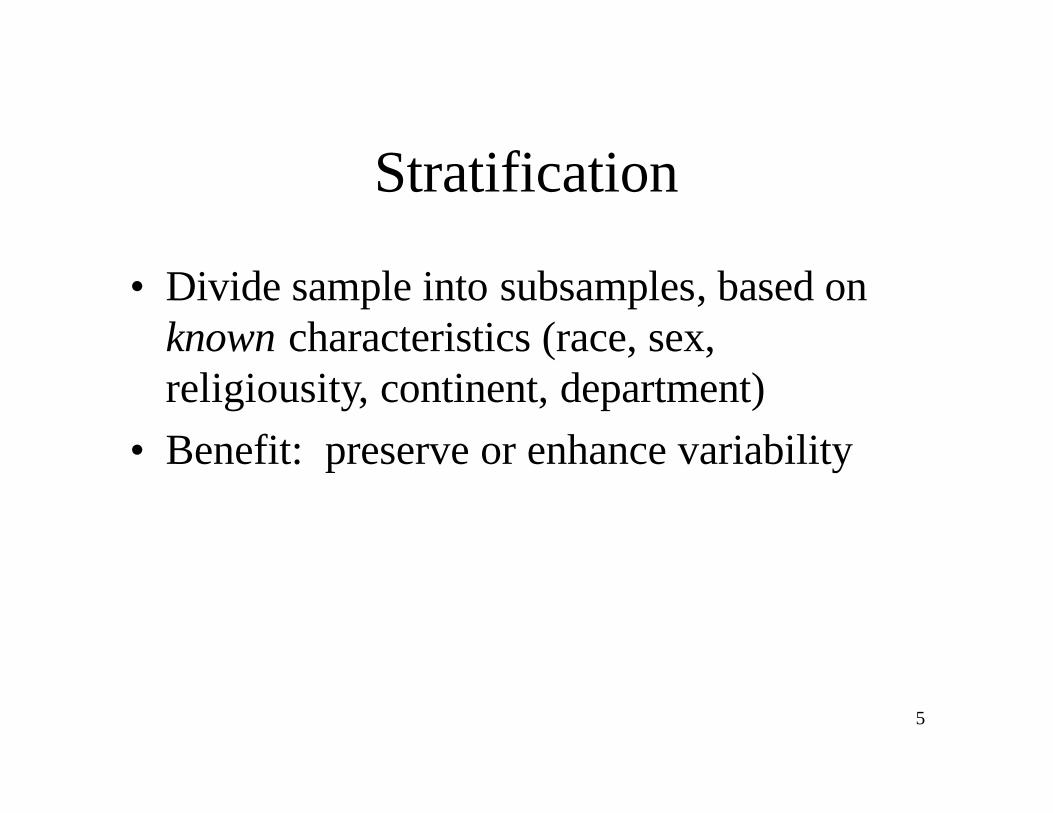
Stratification

• Divide sample into subsamples, based on known characteristics (race, sex, religiousity, continent, department)

• Benefit: preserve or enhance variability

6

Stratification example

0.6%(on 1,487 valid obs.)

1,714Total

n.a.227Missing

Hypothetical sampleNES

2.7%873.4%53Other race/religion

1.3%35017.7%2Black Jews

30

1871,215

N

1.3%3504.6%White Jews

1.3%3501.8%Black Christians1.3%3500.7%White Christians

s.e. @ 50%Ns.e. @ 50%

7

Cluster sampling

Block

HH Unit

Individual

8

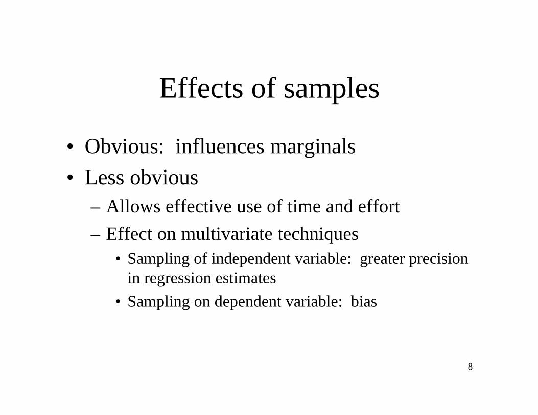
Effects of samples

• Obvious: influences marginals• Less obvious

– Allows effective use of time and effort– Effect on multivariate techniques

• Sampling of independent variable: greater precision in regression estimates

• Sampling on dependent variable: bias

9

Sampling on Independent Variable

x

y

x

y

10

Sampling on Dependent Variable

x

y

x

y

11

Sampling

Consequences for Statistical Inference

12

Statistical Inference:Learning About the Unknown From the

Known• Reasoning forward: distributions of sample

means, when the population mean, s.d., and n are known.

• Reasoning backward: learning about the population mean when only the sample, s.d., and n are known

13

Reasoning Forward

14

Exponential Distribution Example

Fra

ction

inc0 500000 1.0e+06

0

.271441

Mean = 250,000Median=125,000s.d. = 283,474Min = 0Max = 1,000,000

15

Consider 10 random samples, of n = 100 apiece

meanSample

212,137.310

210,593.49

226,422.78

249,036.77

241,369.86

280,657.35

238,928.74

271,074.23

198.789.62

253,396.91

Fra

ctio

n

inc0 250000 500000 1.0e+06

0

.271441

16

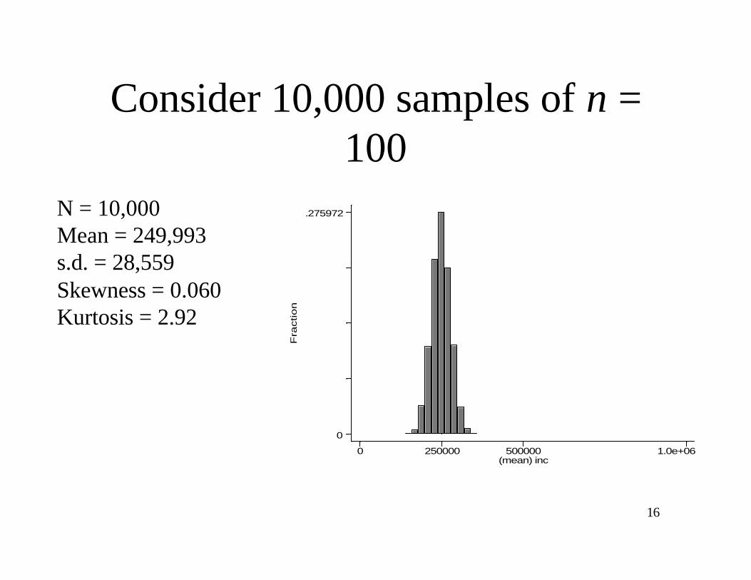
Consider 10,000 samples of n = 100

Fra

ctio

n

(mean) inc0 250000 500000 1.0e+06

0

.275972N = 10,000Mean = 249,993s.d. = 28,559Skewness = 0.060Kurtosis = 2.92

17

Consider 1,000 samples of various sizes

Mean = 249,938s.d.= 9,376Skew= -0.50Kurt= 6.80

Mean = 250,498s.d.= 28,297Skew= 0.02Kurt= 2.90

Mean =250,105s.d.= 90,891Skew= 0.38Kurt= 3.13

100010010

Fra

ctio

n

(mean) inc0 250000 500000 1.0e+06

0

.731

Fra

ctio

n

(mean) inc0 250000 500000 1.0e+06

0

.731

Fra

ctio

n

(mean) inc0 250000 500000 1.0e+06

0

.731

18

Difference of means example

Fra

ctio

n

inc0 250000 500000 1.0e+06

0

.280203

Fra

ctio

n

inc20 250000 500000 1.0e+06

0

.251984

State 1Mean = 250,000

State 2Mean = 300,000

19

Take 1,000 samples of 10, of each state, and compare them

First 10 samples

><

<<

<>

<>

<

<

152,312222,72510314,882152,6789

333,208253,8858210,970127,1157

284,309270,4006189,674220,9345

557,909253,3744438,336468,5743

243,062184,5712

365,224311,4101

State 2State 1Sample

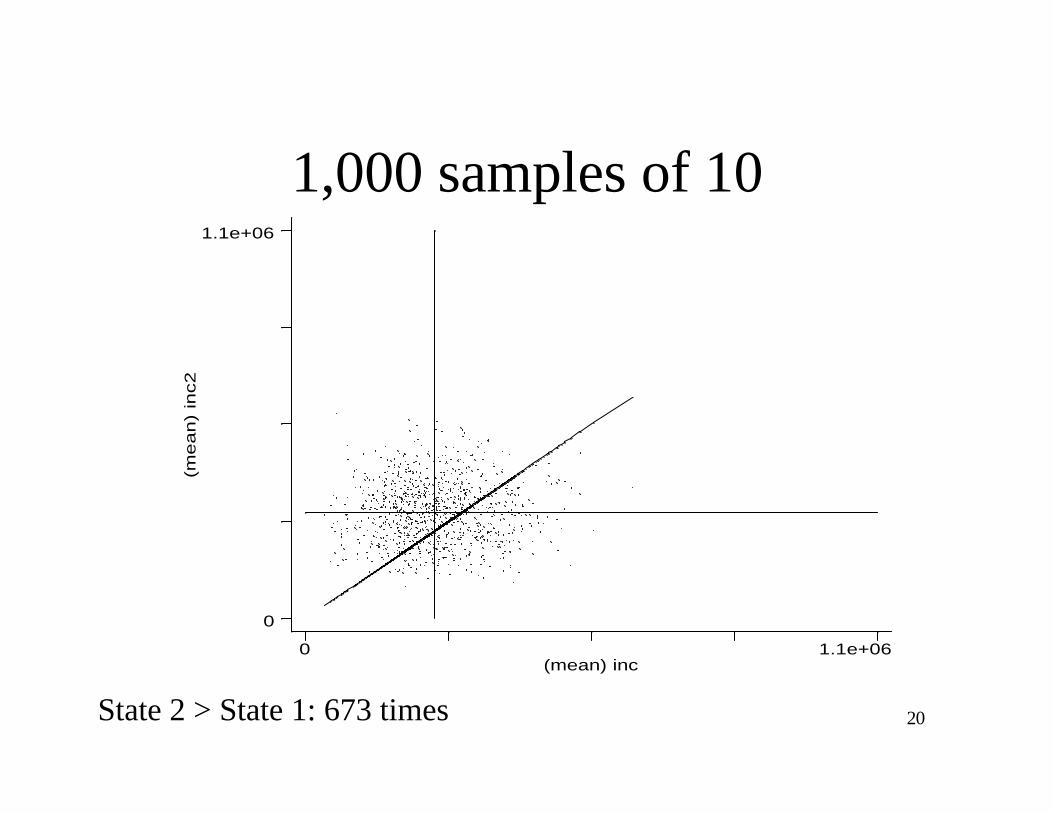
20

1,000 samples of 10(m

ea

n)

inc2

(mean) inc0 1.1e+06

0

1.1e+06

State 2 > State 1: 673 times

21

1,000 samples of 100(m

ea

n)

inc2

(mean) inc0 1.1e+06

0

1.1e+06

State 2 > State 1: 909 times

22

1,000 samples of 1,000

State 2 > State 1: 1,000 times

(me

an

) in

c2

(mean) inc0 1.1e+06

0

1.1e+06

23

Another way of looking at it:The distribution of Inc2 – Inc1

Mean = 49,816s.d. = 13,932

Mean = 49,704s.d. = 38,774

Mean = 51,845s.d. = 124,815

n = 1,000n = 100n = 10

Fra

ctio

n

diff-400000 0 600000

0

.565

Fra

ctio

n

diff-400000 050000 600000

0

.565

Fra

ctio

n

diff-400000 050000 600000

0

.565

24

Reasoning Backward

µabout somethingsay obut want t , and ,X , knowyou When sn

25

Central Limit Theorem

As the sample size n increases, the distribution of the mean of a random sample taken from practically any population approaches a normaldistribution, with mean : and standard deviation

X

nσ

26

Calculating Standard Errors

In general:

ns

=err. std.

27

Most important standard errors

Regression (slope) coeff.

Diff. of 2 means

Proportion

Meanns

npp )1( −

21

11nn

s p +

xsnres 1... ×

28

If you know the sample mean, s.d., and n, what can you say about the population

mean?

error standard intervalarbitrary mean sample mean population

general,In

×±=

29

If n is sufficiently large, choose the interval using the normal curve

y

Mean

.000134

.398942

σ σ2 σ3 σ4σ−σ2−σ3−σ4− 68%

95%99%

30

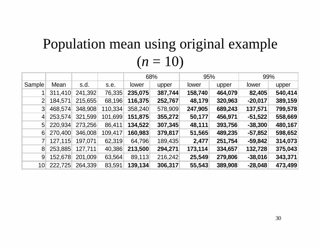
Population mean using original example (n = 10)

Sample Mean s.d. s.e. lower upper lower upper lower upper1 311,410 241,392 76,335 235,075 387,744 158,740 464,079 82,405 540,4142 184,571 215,655 68,196 116,375 252,767 48,179 320,963 -20,017 389,1593 468,574 348,908 110,334 358,240 578,909 247,905 689,243 137,571 799,5784 253,574 321,599 101,699 151,875 355,272 50,177 456,971 -51,522 558,6695 220,934 273,256 86,411 134,522 307,345 48,111 393,756 -38,300 480,1676 270,400 346,008 109,417 160,983 379,817 51,565 489,235 -57,852 598,6527 127,115 197,071 62,319 64,796 189,435 2,477 251,754 -59,842 314,0738 253,885 127,711 40,386 213,500 294,271 173,114 334,657 132,728 375,0439 152,678 201,009 63,564 89,113 216,242 25,549 279,806 -38,016 343,371

10 222,725 264,339 83,591 139,134 306,317 55,543 389,908 -28,048 473,499

68% 95% 99%

31

Population mean using original example (n = 1000)

Sample Mean s.d. s.e. lower upper lower upper lower upper1 238,226 277,492 8,775 229,450 247,001 220,675 255,776 211,900 264,5512 260,658 290,954 9,201 251,458 269,859 242,257 279,060 233,056 288,2613 253,374 277,022 8,760 244,614 262,134 235,853 270,894 227,093 279,6554 242,002 283,772 8,974 233,028 250,975 224,055 259,949 215,081 268,9235 244,437 279,343 8,834 235,603 253,271 226,770 262,104 217,936 270,9386 248,896 279,213 8,829 240,067 257,726 231,237 266,555 222,408 275,3857 267,218 291,150 9,207 258,011 276,425 248,804 285,632 239,597 294,8398 244,138 276,490 8,743 235,394 252,881 226,651 261,624 217,908 270,3689 247,996 275,994 8,728 239,268 256,723 230,540 265,451 221,813 274,179

10 255,023 287,118 9,079 245,944 264,103 236,864 273,182 227,785 282,262

68% 95% 99%

32

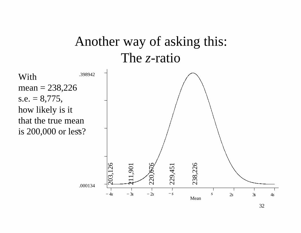
Another way of asking this:The z-ratio

Withmean = 238,226s.e. = 8,775, how likely is itthat the true meanis 200,000 or less?y

Mean

.000134

.398942

σ σ2 σ3 σ4σ−σ2−σ3−σ4−23

8,22

6

229,

451

220,

676

211,

901

203,

126

33

Z

37.48,775

200,000) - (238,226z

case, in this

,error standard

)test value-mean (Sample

==

=z

34

t (when the sample is small)

z-4 -2 0 2 4

.000045

.003989

t-distribution

z (normal) distribution

35

Reading a z table

36

Reading a t table

37

Doing a t-testQ: How likely is it that the residual vote rate n 1996 was 2.5%or less?

Fra

ctio

n

blank960 .025 .1 .2 .3

0

.2

Mean: 0.02618s.d.: 0.02140N: 1905

00049.01905/02140.0

/..

==

= nses

38

The pictureMean: 0.02618s.d.: 0.02140N: 1905

00049.01905/02140.0

/..

==

= nsesy

newz.026181.02569.0252

.000134

.398942

408.200049.0

025.026181.0

=

−=t

39

The STATA output

. ttest blank96=.025

One-sample t test

------------------------------------------------------------------------------

Variable | Obs Mean Std. Err. Std. Dev. [95% Conf. Interval]

---------+--------------------------------------------------------------------

blank96 | 1905 .0261806 .0004903 .0213979 .0252191 .0271421

------------------------------------------------------------------------------

Degrees of freedom: 1904

Ho: mean(blank96) = .025

Ha: mean < .025 Ha: mean ~= .025 Ha: mean > .025

t = 2.4082 t = 2.4082 t = 2.4082

P < t = 0.9919 P > |t| = 0.0161 P > t = 0.0081

40

Doing another t-testQ: How likely is it that the residual vote rate in 1996 equal to the rate in 1992 (I.e., blank96-blank92= 0)?

Fra

ctio

n

diff9692-.2 0 .2 .4

0

.429558

Mean: 0.003069s.d.: 0.02323N: 1448

00061.01448/02323.0

/..

==

= nses

41

The picture

028.500061.0

0003069.0

=

−=t

Mean: 0.003069s.d.: 0.02323N: 1448

00061.01448/02323.0

/..

==

= nsesy

newz.003069.00246.00185.00124.000627.000017-.00059

.000134

.398942

42

The STATA output. ttest blank96=blank92Paired t test------------------------------------------------------------------------------Variable | Obs Mean Std. Err. Std. Dev. [95% Conf. Interval]---------+--------------------------------------------------------------------blank96 | 1448 .0242941 .0005116 .0194689 .0232904 .0252977blank92 | 1448 .021225 .0005382 .0204813 .0201692 .0222808---------+--------------------------------------------------------------------

diff | 1448 .003069 .0006104 .0232279 .0018717 .0042664------------------------------------------------------------------------------

Ho: mean(blank96 - blank92) = mean(diff) = 0Ha: mean(diff) < 0 Ha: mean(diff) ~= 0 Ha: mean(diff) > 0

t = 5.0278 t = 5.0278 t = 5.0278P < t = 1.0000 P > |t| = 0.0000 P > t = 0.0000

. ttest diff9692=0One-sample t test------------------------------------------------------------------------------Variable | Obs Mean Std. Err. Std. Dev. [95% Conf. Interval]---------+--------------------------------------------------------------------diff9692 | 1448 .003069 .0006104 .0232279 .0018717 .0042664------------------------------------------------------------------------------Degrees of freedom: 1447

Ho: mean(diff9692) = 0Ha: mean < 0 Ha: mean ~= 0 Ha: mean > 0t = 5.0278 t = 5.0278 t = 5.0278

P < t = 1.0000 P > |t| = 0.0000 P > t = 0.0000.

43

Final t-testQ: Was there a relationship between residual vote and countySize in 1996?

Slope coeff: -0.07510s.e.r: 0.7115N: 1861Sx: 1.4788

01115.06762.001649.0

4788.11

18617115.0

1....

=×=

×=

×=xsn

reses

blan

k96

vap96_to

blank96 Fitted values

326 6.5e+06

.000281

.298789

44

Calculating t

7319.601115.

07510.0

−=

−=t

45

The STATA output

. reg lblank96 lvap96

Source | SS df MS Number of obs = 1861-------------+------------------------------ F( 1, 1859) = 45.32

Model | 22.941515 1 22.941515 Prob > F = 0.0000Residual | 941.080329 1859 .506229332 R-squared = 0.0238

-------------+------------------------------ Adj R-squared = 0.0233Total | 964.021844 1860 .518291314 Root MSE = .7115

------------------------------------------------------------------------------lblank96 | Coef. Std. Err. t P>|t| [95% Conf. Interval]

-------------+----------------------------------------------------------------lvap96 | -.0750985 .0111556 -6.73 0.000 -.0969774 -.0532197_cons | -3.129858 .1113781 -28.10 0.000 -3.348298 -2.911419

------------------------------------------------------------------------------