Sampling-based Path Planning on Configuration-Space CostmapsLeonard Jaillet, Juan Cortes and Thierry Simeon

Abstract—This paper addresses path planning considering acost function defined over the configuration space. The proposedTransition-based RRT planner computes low-cost paths that fol-low valleys and saddle points of the configuration-space costmap.It combines the exploratory strength of RRTs with transition testsused in stochastic optimization methods to accept or to reject newpotential states. The planner is analyzed and shown to computelow-cost solutions with respect to a path quality criterion basedon the notion of mechanical work. A large set of experimentalresults is provided to demonstrate the effectiveness of the method.Current limitations and possible extensions are also discussed.

I. INTRODUCTION

Sampling-based path planning has proven to be an effectiveframework suitable for a large class of problems in domainssuch as robotics, manufacturing, computer animation and com-putational biology (see [1], [2] for a survey). These techniqueshandle complex problems in high-dimensional spaces butusually operate in a binary world aiming to find out collision-free solutions rather than the optimal path.

Specific path planning methods have been developed infield robotics for outdoor navigation, where the goal is to findoptimal paths according to a cost function, usually computedfrom a model of the terrain. Classical grid-based methods suchas A* or D* [3] can be used to compute resolution-optimalpaths over a costmap. However, compared to sampling-basedalgorithms, these methods are limited to problems involvinglow-dimensional spaces that can be discretized and searchedusing grid search techniques.

Some recent works [4]–[8] have tried to bridge the gapbetween sampling-based planners and grid-based costmapplanners. They mainly rely on the RRT algorithm [9], andare generally focused on specific applications (e.g. real timeproblems [7], [10] or statistical learning of feasible paths [8])in the context of 2D robot navigation problems.

This paper presents a general algorithm, called Transition-based RRT (T-RRT),1 for path planning on configuration-spacecostmaps. The algorithm considers a user-given cost functiondefined over the configuration space as an additional input tothe standard path planning problem, and it produces solutionpaths that are not only feasible (e.g. collision-free), but alsohave a good quality with respect to the input costmap. Forinstance, the costmap may correspond in outdoor navigation

Leonard Jaillet is with the Institut de Robotica i Informatica IndustrialCSIC-UPC; c/ Llorens i Artigas 4-6, 08028 Barcelona, Spain (e-mail: ljail-let@iri.upc.edu). Juan Cortes and Thierry Simeon are with CNRS; LAAS; 7avenue du colonel Roche, F-31077 Toulouse, France, and with Universite deToulouse; UPS, INSA, INP, ISAE; LAAS; F-31077 Toulouse, France (e-mail:jcortes@laas.fr; nic@laas.fr).

1The T-RRT planner was introduced in a shorter version published in [11].

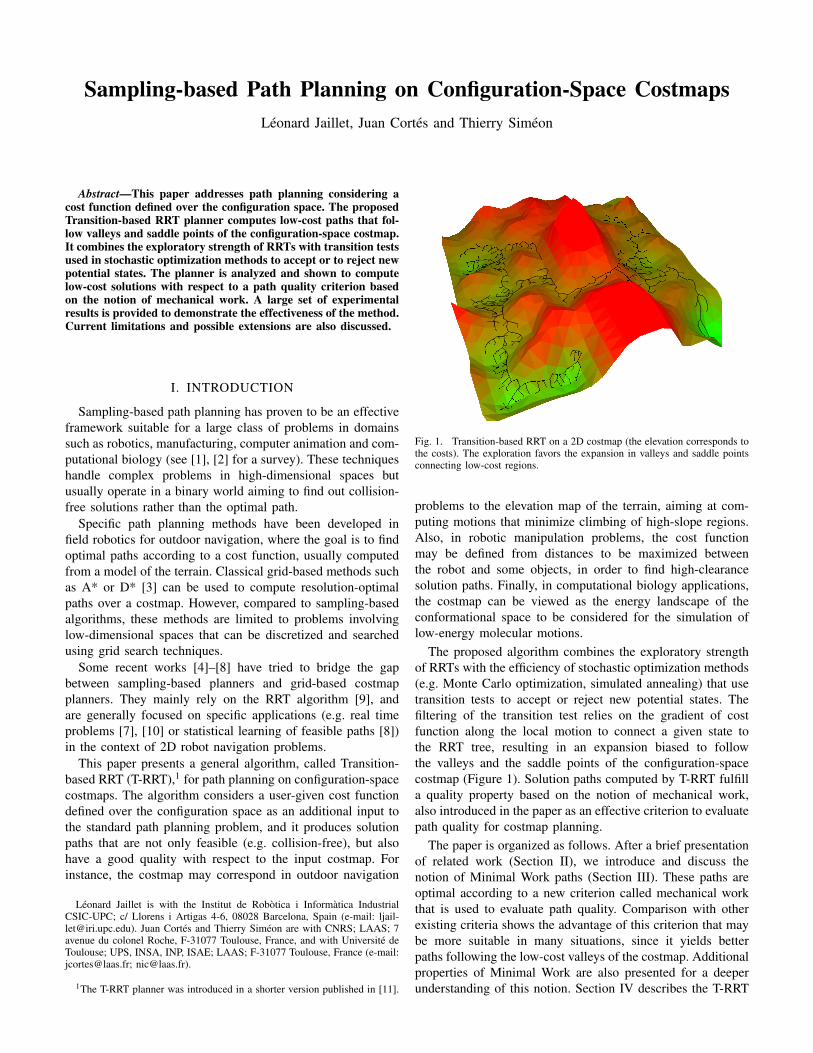
Fig. 1. Transition-based RRT on a 2D costmap (the elevation corresponds tothe costs). The exploration favors the expansion in valleys and saddle pointsconnecting low-cost regions.

problems to the elevation map of the terrain, aiming at com-puting motions that minimize climbing of high-slope regions.Also, in robotic manipulation problems, the cost functionmay be defined from distances to be maximized betweenthe robot and some objects, in order to find high-clearancesolution paths. Finally, in computational biology applications,the costmap can be viewed as the energy landscape of theconformational space to be considered for the simulation oflow-energy molecular motions.

The proposed algorithm combines the exploratory strengthof RRTs with the efficiency of stochastic optimization methods(e.g. Monte Carlo optimization, simulated annealing) that usetransition tests to accept or reject new potential states. Thefiltering of the transition test relies on the gradient of costfunction along the local motion to connect a given state tothe RRT tree, resulting in an expansion biased to followthe valleys and the saddle points of the configuration-spacecostmap (Figure 1). Solution paths computed by T-RRT fulfilla quality property based on the notion of mechanical work,also introduced in the paper as an effective criterion to evaluatepath quality for costmap planning.

The paper is organized as follows. After a brief presentationof related work (Section II), we introduce and discuss thenotion of Minimal Work paths (Section III). These paths areoptimal according to a new criterion called mechanical workthat is used to evaluate path quality. Comparison with otherexisting criteria shows the advantage of this criterion that maybe more suitable in many situations, since it yields betterpaths following the low-cost valleys of the costmap. Additionalproperties of Minimal Work are also presented for a deeperunderstanding of this notion. Section IV describes the T-RRT

algorithm, including the methods for self-tuning of parametersand for the expansion rate control. Section V shows how T-RRT implicitly computes Minimal Work paths and discussesits probabilistic completeness. An experimental validation ofthe planner is conducted in Section VI. The overall efficacyof T-RRT is shown on different problems and positivelycompared with other existing techniques [4], [6]. This sectionalso analyzes the influence of the intrinsic parameters of thealgorithm on the overall performance, and results indicate thatno specific tuning is actually needed. Section VII presentssome extensions of T-RRT, and conclusions are outlined inSection VIII.

II. RELATED WORK

Early potential field methods [12], as well as their com-bination with strategies for escaping local minima, e.g. therandomized planner of [13], rely on some numerical fielddefined over the configuration space that may be viewed asa specific kind of costmap. Note however that the artificialpotential field of these methods is only defined as a wayfor planning collision-free paths, without considering pathoptimality. Thus, these methods do not address the problemconsidered here of computing low-cost, feasible paths from anarbitrarily complex costmap given as input to the planner.

Recent sampling-based planners have proven to be veryeffective at finding feasible solutions that can be locallyoptimized in a post-processing stage. Local path optimizationmethods such as the shortcut algorithm [14] are generallyused to improve path quality with respect to simple criteria,like path length, clearance, or a combination of both [15].These smoothing methods only aim to locally improve asolution path, as opposed to the global exploration algorithmproposed in the paper. Moreover, their extension to arbitrarycost functions has not yet been addressed, and the resultingefficacy of such extension remains to be further evaluated.

Only few papers consider sampling-based path planningon arbitrary cost spaces. In [4], an adaptation of the RRT-Connect planner is used to find low-cost paths for rough terrainnavigation. The idea is to keep new configurations only if theircost is under a given threshold, first initialized to a low value,and then iteratively increased during the search. One limitationof this technique comes from the non-decreasing threshold,which limits the efficiency of low-cost search to the vicinityof the root nodes. To overcome this issue, the extensionproposed in [5] considers multiple RRTs trees grown fromrandomly sampled root configurations. However, this solutionstill expects an appropriate number of initial samples in orderto get enough low-cost seeds among the space. Moreover, itrequires a manual tuning of the parameter that controls thecost threshold growth rate. This tuning is highly problem-dependent.

In [6], the heuristically-guided RRT (hRRT) biases thesearch using a quality measure based on the integral of thecost along the path from the root node and an estimation ofthe optimal cost to the goal. Such an approach, inspired fromgraph search techniques, can also be found in the contextof real-time applications [7], [10] and statistical learning

of feasible paths [8]. However, with these techniques, theestimated cost to goal is heuristic and tends to bias thesearch straight toward the goal at the expense of lower-qualitysolution paths. Moreover, the aforementioned methods haveonly been demonstrated on simple low-dimensional exampleswith discrete cost states (invalid, low cost, high cost). Theirscalability and performance for problems involving complexcost spaces in higher dimensions are yet to be established.

The T-RRT algorithm introduced below is inspired byMonte Carlo optimization techniques. Developed in order tofind global optima in very complex spaces [16], they introducerandomness as a means to avoid local minima traps. Manyvariants have been developed (e.g. random walk, simulatedannealing [17]). The basic exploration process typically relieson successive transition tests, performed using the Metropoliscriterion (see Section IV-B). Note also that the ProbabilisticConformational Roadmap [18] developed for exploring molec-ular energy landscapes in computational biology applicationsintegrates a similar transition test in the PRM framework [19].

III. MINIMAL WORK PATHS

This section introduces the mechanical work criterion tomeasure path quality in a space that is mapped by a givencost function. Paths that are optimal according to this criterionare called Minimal Work (MW) paths. The T-RRT algorithmpresented in the next section tends to produce such MW paths,as shown by the theoretical analysis and the experimental re-sults in Sections V and VI respectively. First, we introduce thenotion of MW paths and illustrate how this criterion generallyyields more natural solution paths (i.e. paths following well thelow-cost valleys of the costmap) compared to other existingpath quality measures.

A. Notation

Let us consider a system with a configuration space C,possibly constrained by “binary” obstacle regions. Let us alsoconsider a cost function c : C→ R∗+ mapping this space, i.e.a cost c(q) > 0 can be computed for each q ∈ C. This costfunction c is assumed to be continuous. A path P of length l isrepresented by a unit-speed parametric function2 τ : [0, l]→ C

with τ(s) = qs ∈ P. Then, we define the parametric costfunction v : [0, l]→ R∗+ of a path as v(s) = c◦ τ(s) = c(qs).

B. Classical Path Quality Measures

Several criteria have been proposed to evaluate the qualityof a path from its parametric cost function, e.g. maximalcost [5], average cost [5]–[7], or costs sum over discrete pathconfigurations [5], [8] (as a way to approximate the integralof the cost along the path). The maximal cost criterion isthe most limited one since it only relies on a point value ofthe parameterized cost function. The average cost can also bemisleading since it does not account for path length (a pathinvolving many detours inside a low-cost region will have anaverage cost smaller than a path going straight through this

2This representation assumes that the parameterized curve representing thepath is regular, which simplifies the notation.

Fig. 2. Decomposition of a path into portions of monotonic cost variation. αi

and βi correspond respectively to local minima and maxima. The mechanicalwork (right) is the sum of positive cost variations between consecutive extremaplus a small value εl proportional to the path length.

region). Thus, the integral of the cost along a path appears tobe a more reliable criterion. It is mathematically defined as:

S(P) =∫ l

0

v(s)ds.

A discrete approximation of the integral leads to:

S(P) ∼ l

n

n−1∑k=0

v(sk), with sk =(

k

n− 1

)l.

In what follows, optimal paths according to the Integral of theCost criterion are called IC Paths. The next section introducesan alternative way for measuring path quality based on thenotion of mechanical work.This alternative technique will thenbe compared to IC paths in Subsection III-D.

C. Mechanical Work of a Path

The key idea is that positive variations of the parametriccost function can be seen as forces acting against motion andthus producing mechanical work. We propose to use this lossof “energy” induced by the mechanical work for measuring thequality of a path. In the case of negative variation of costs,the system does not lose any energy. Then, a small penaltyproportional to the distance is added in order to favor shortestpaths of equal mechanical energy. Based on this principle, themechanical work of a path is defined as:

W (P) =∫

P+

∂v

∂sds+ ε

∫P

ds, (1)

where P+ represents the portions of path with positive slopes(i.e. where the parametric cost function is strictly increasing),and ε is assumed to be very low compared to cost values.

The continuous expression of W in Equation (1) can betransformed into a discrete formulation expressed from thelocal extrema values along the path:

W (P) =∑

i

(v(βi)− v(αi)) + εl

=∑

i

∆v+i + εl,

(2)

Fig. 3. Minimal Work solution paths. The paths are computed using the A∗algorithm within a 2D grid discretizing the space (a). The examples illustraterespectively down-to-down (b), top-to-top (c), and top-to-down (d) queries.

where αi and βi are consecutive minima and maxima of thecosts along the paths and ∆v+

i = v(βi)−v(αi) are the positivevariations between two consecutive extrema (Figure 2). Themechanical work of a path is simply obtained by summing upthe positive differences between extrema of its parameterizedcost function and adding εl in order to favor shortest pathsamong the ones having equally positive cost variations. Pathsthat minimize the mechanical work for a given query are calledMinimal Work (MW) paths.

Figure 3 shows examples of MW paths for several querieson a 2D hilly costmap. The paths were computed using astandard A∗ search performed on a grid discretizing the two-dimensional landscape. As one can see, the shapes of the MWpaths appear to be suitable in the sense that they follow asmuch as possible the low-cost regions of the space. In orderto better state the pertinence of the mechanical work criterion,we first compare it with the IC criterion in the next subsection.Then, we state some interesting properties of the MW criterionin Subsection III-E.

D. Minimal Work vs. Integral of the Cost

This section compares the optimal solutions for the integralof the cost S (IC paths) and for the mechanical work W(MW paths) on representative cost spaces.

1) Constant Slope: Let us first consider the example ofa planar landscape with a constant slope. In this simplecase, IC solutions can be numerically characterized fromcalculus of variations. As shown in Figure 4, the solutionsobtained for two different slopes show that IC paths (inblack) are not intuitive and moreover depend on the planeinclination. In contrast, the MW path is in both cases thetrivial straight-line path (in blue). Indeed, the cost of MWpaths is always lower-bounded by the cost variation betweenthe initial and final configurations. In situations for which thequery configurations can be connected through a set of pathshaving a monotonic cost variation (as for the specific case ofa constant slope landscape), the MW path will be the shortest

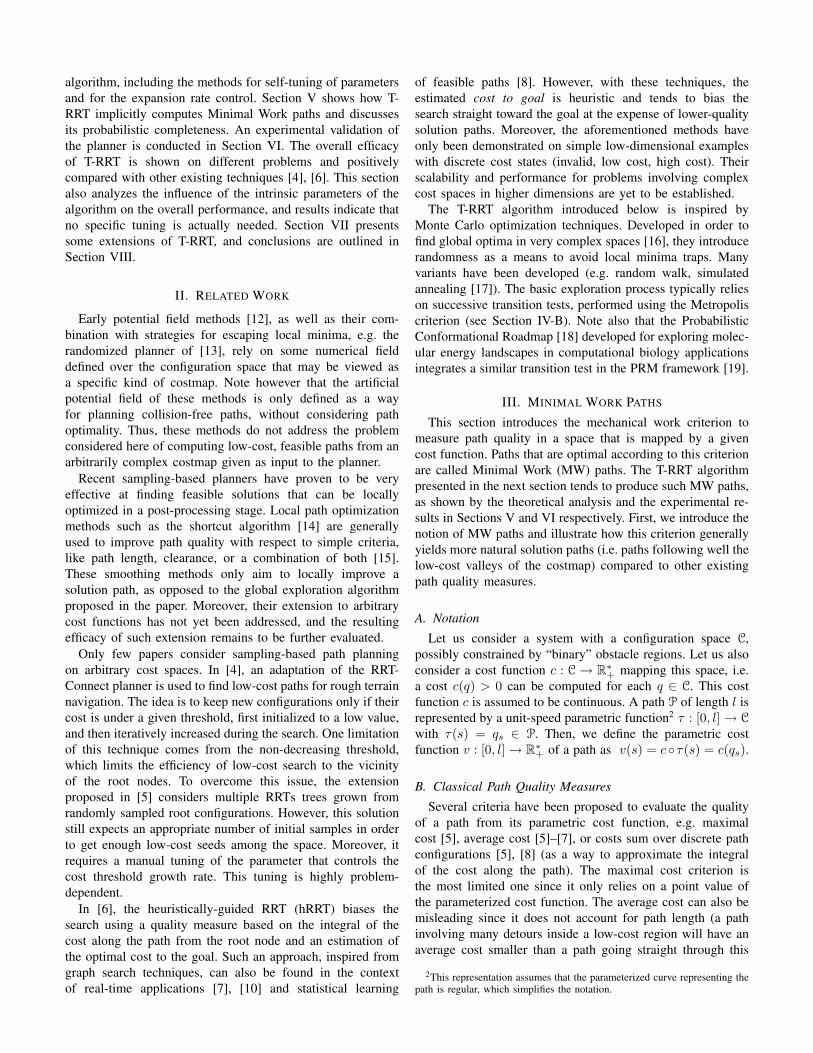
Fig. 4. The straight-line MW path (blue) and two different IC paths for twodifferent inclinations of the plane representing the cost function.

Fig. 5. High-cost barrier problem: (a) MW path, (b) IC path.

one among the set of minimal cost variation paths, yielding astraight-line solution for the planar slope example.

2) High-Cost Barrier: This example corresponds to a flatcost surface with a high-cost barrier that should be preferablyavoided (Figure 5). In this case, the MW path is the shortestpath getting around the barrier (Figure 5a) while the ICsolution is a direct path that crosses the barrier (Figure 5b).This example highlights another possibly negative feature ofthe integral of the cost criterion that may favor undesirablepaths with short high-cost portions.

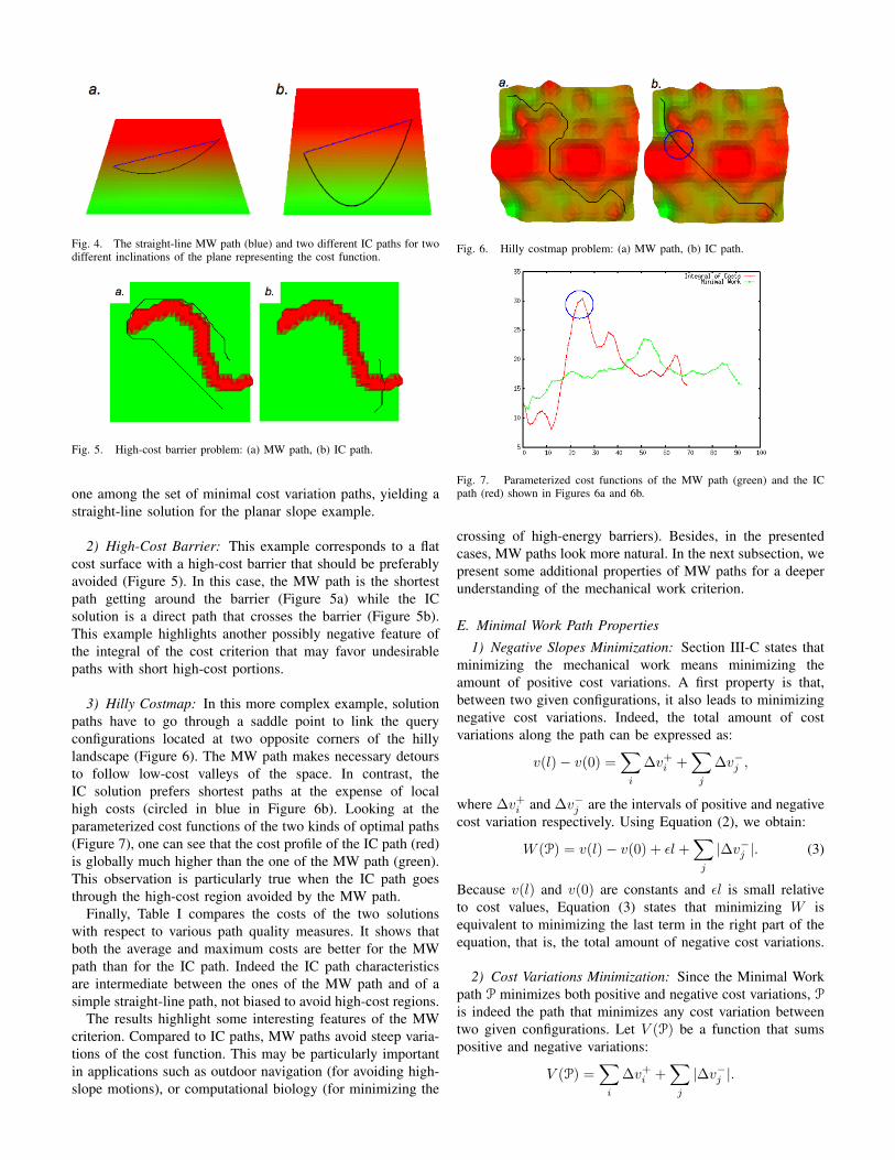
3) Hilly Costmap: In this more complex example, solutionpaths have to go through a saddle point to link the queryconfigurations located at two opposite corners of the hillylandscape (Figure 6). The MW path makes necessary detoursto follow low-cost valleys of the space. In contrast, theIC solution prefers shortest paths at the expense of localhigh costs (circled in blue in Figure 6b). Looking at theparameterized cost functions of the two kinds of optimal paths(Figure 7), one can see that the cost profile of the IC path (red)is globally much higher than the one of the MW path (green).This observation is particularly true when the IC path goesthrough the high-cost region avoided by the MW path.

Finally, Table I compares the costs of the two solutionswith respect to various path quality measures. It shows thatboth the average and maximum costs are better for the MWpath than for the IC path. Indeed the IC path characteristicsare intermediate between the ones of the MW path and of asimple straight-line path, not biased to avoid high-cost regions.

The results highlight some interesting features of the MWcriterion. Compared to IC paths, MW paths avoid steep varia-tions of the cost function. This may be particularly importantin applications such as outdoor navigation (for avoiding high-slope motions), or computational biology (for minimizing the

Fig. 6. Hilly costmap problem: (a) MW path, (b) IC path.

Fig. 7. Parameterized cost functions of the MW path (green) and the ICpath (red) shown in Figures 6a and 6b.

crossing of high-energy barriers). Besides, in the presentedcases, MW paths look more natural. In the next subsection, wepresent some additional properties of MW paths for a deeperunderstanding of the mechanical work criterion.

E. Minimal Work Path Properties

1) Negative Slopes Minimization: Section III-C states thatminimizing the mechanical work means minimizing theamount of positive cost variations. A first property is that,between two given configurations, it also leads to minimizingnegative cost variations. Indeed, the total amount of costvariations along the path can be expressed as:

v(l)− v(0) =∑

i

∆v+i +

∑j

∆v−j ,

where ∆v+i and ∆v−j are the intervals of positive and negative

cost variation respectively. Using Equation (2), we obtain:

W (P) = v(l)− v(0) + εl +∑

j

|∆v−j |. (3)

Because v(l) and v(0) are constants and εl is small relativeto cost values, Equation (3) states that minimizing W isequivalent to minimizing the last term in the right part of theequation, that is, the total amount of negative cost variations.

2) Cost Variations Minimization: Since the Minimal Workpath P minimizes both positive and negative cost variations, P

is indeed the path that minimizes any cost variation betweentwo given configurations. Let V (P) be a function that sumspositive and negative variations:

V (P) =∑

i

∆v+i +

∑j

|∆v−j |.

Length Cave Cmax S WMW path 186 17.9 23.6 3324 15.9IC path 139 18.6 30.4 2592 32.5Str. Line 127 22.6 39.6 2877 41.0

TABLE IMW AND IC OPTIMAL PATHS OF FIGURE 6 COMPARED TO A REFERENCE

STRAIGHT-LINE SOLUTION.

Using Equations (2) and (3), we get:

V (P) = 2.W (P)− (v(l)− v(0) + 2εl). (4)

Thus, the ordering of the paths remains the same regardlessof the criterion (V or W ), which, indeed, means that theyare equivalent. However we will keep the formulation ofMinimal Work path since this notion facilitates the analysisof the T-RRT algorithm.

3) Reversibility of Minimal Work Paths: Let −1P be thereverse path of P. Since the parametric cost functions v and−1v have opposed variations, i.e. ∆−1v+ = |∆v−|, we have:

W (−1P) =∑

j

|∆v−j |+ εl,

and using Equation (3), we get:

W (−1P) = W (P) + v(0)− v(l). (5)

Consequently, the mechanical work of a path is equal to themechanical work of its inverse, except for a constant. Thisproperty allows us to speak about the MW path between twoconfigurations without the need for orienting the path.

IV. TRANSITION-BASED RRT

A. Main Algorithm

The T-RRT algorithm combines the advantages of twomethods. First, it benefits from the exploratory strength ofRRT-like algorithms resulting from their expansion bias towardlarge Voronoi regions of the space. Additionally, it integratesfeatures of stochastic optimization methods developed forcomputing global minima in complex spaces: it uses transitiontests to accept or reject potential states.

Algorithm 1 shows the pseudo-code of the T-RRT planner.Similarly to the Extend version of the basic RRT algorithm[20], a randomly sampled configuration qrand is used todetermine both the nearest tree node qnear to be extendedand the extension direction. The extension from qnear isperformed toward qrand with an increment step δ. In thecase of T-RRT, δ has to be small enough to avoid cost picksto be missed by the linear interpolation between qnear andqnew. This stage also integrates collision detections in thepresence of “binary obstacles.” Thus, if the new portion ofpath leads to a collision, a null configuration is returned andthe extension fails, independently of the associated costs. Thisextension process ensures the bias toward unexplored freeregions of the space. The goal of the second stage is tofilter irrelevant configurations regarding the search of low-cost paths before inserting qnew in the tree. Such filteringis performed by the TransitionTest function. It relies

Algorithm 1: Transition-based RRT

input : the configuration space C;the cost function c : C→ R∗+;the root qinit and the goal qgoal;

output : the tree T ;beginT ← InitTree(qinit);while not StopCondition(T , qgoal) do

qrand ← SampleConf(C) ;qnear ← NearestNeighbor(qrand, T );qnew ← Extend(T , qrand, qnear);if qnew 6= NULLand TransitionTest(c(qnear), c(qnew), dnear−new)and MinExpandControl(T , qnear, qrand) then

AddNewNode(T , qnew);AddNewEdge(T , qnear, qnew);

end

on the Metropolis criterion commonly used in stochastic opti-mization methods. This test integrates a self-tuning techniquein order to automatically control its filtering strength, andthus to ensure continuous growth of the tree. Finally,the MinExpandControl function forces the planner tomaintain a minimal rate of expansion toward unexploredregions of the space, and avoids possible blocking situa-tions during the search. The following subsections detail theTransitionTest and MinExpandControl functions.

B. Transition Test

The TransitionTest function is presented in Algo-rithm 2. First, configurations with a higher cost than themaximum cost threshold cmax are filtered. The probability ofacceptance of a new configuration is defined by comparing itscost cj relatively to the cost ci of its parent in the tree. Thistest is based on the Metropolis criterion initially introducedin statistical physics and molecular modeling. The transitionprobability pij is defined as:

pij ={

exp(−∆cij

K·T ) if ∆cij > 0,1 otherwise,

(6)

where:• ∆cij = cj−ci

dij, is the slope of the cost, i.e. the cost varia-

tion divided by the distances between the configurations.3

• K is a constant value used to normalize the expression.It is based on the order of magnitude of the consideredcosts. K is taken as the average cost of the queryconfigurations since they are the only cost values knownat the beginning of the search process.

• T is a parameter called temperature that is used to controlthe difficulty level of transition tests, as further explainedbelow. Note that the term temperature is employed inanalogy with methods in statistical physics, but in ourcase it does not have any physical meaning.

3Contrarily to classical Monte Carlo methods, the cost variation is normal-ized by the distance to the previous state since this distance is not necessarilyconstant.

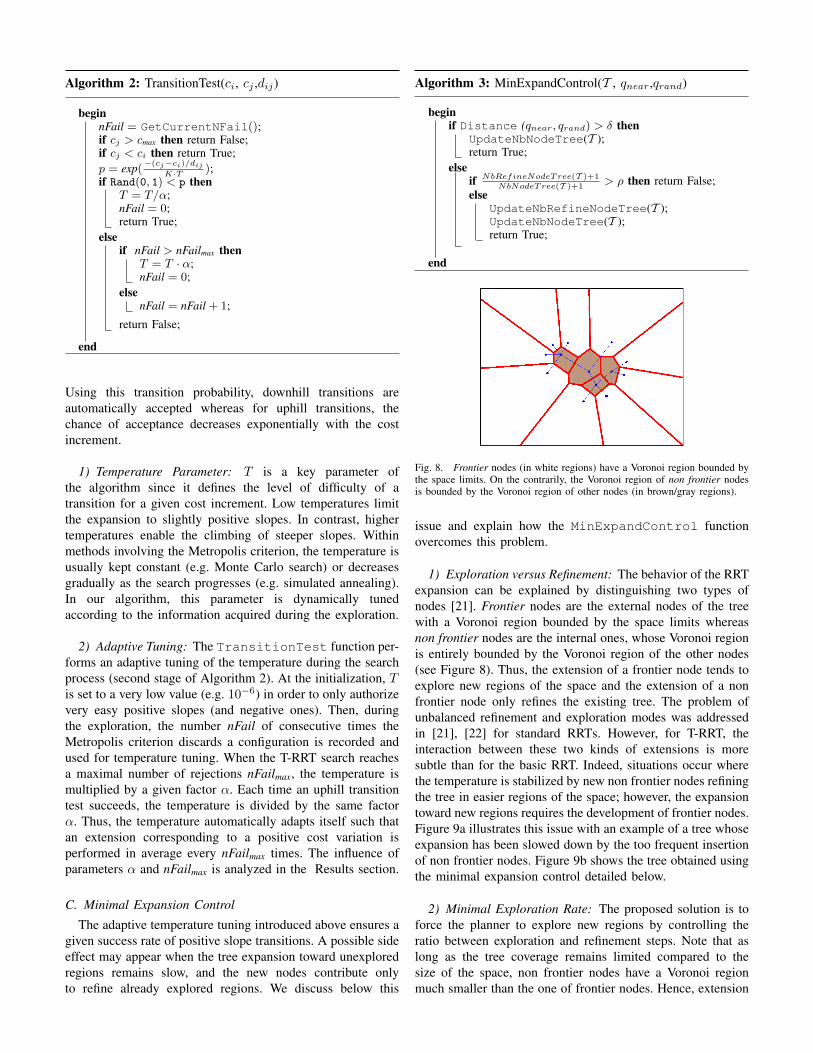
Algorithm 2: TransitionTest(ci, cj ,dij)

beginnFail = GetCurrentNFail();if cj > cmax then return False;if cj < ci then return True;p = exp(

−(cj−ci)/dij

K·T );if Rand(0, 1) < p then

T = T/α;nFail = 0;return True;

elseif nFail > nFailmax then

T = T · α;nFail = 0;

elsenFail = nFail + 1;

return False;

end

Using this transition probability, downhill transitions areautomatically accepted whereas for uphill transitions, thechance of acceptance decreases exponentially with the costincrement.

1) Temperature Parameter: T is a key parameter ofthe algorithm since it defines the level of difficulty of atransition for a given cost increment. Low temperatures limitthe expansion to slightly positive slopes. In contrast, highertemperatures enable the climbing of steeper slopes. Withinmethods involving the Metropolis criterion, the temperature isusually kept constant (e.g. Monte Carlo search) or decreasesgradually as the search progresses (e.g. simulated annealing).In our algorithm, this parameter is dynamically tunedaccording to the information acquired during the exploration.

2) Adaptive Tuning: The TransitionTest function per-forms an adaptive tuning of the temperature during the searchprocess (second stage of Algorithm 2). At the initialization, Tis set to a very low value (e.g. 10−6) in order to only authorizevery easy positive slopes (and negative ones). Then, duringthe exploration, the number nFail of consecutive times theMetropolis criterion discards a configuration is recorded andused for temperature tuning. When the T-RRT search reachesa maximal number of rejections nFailmax, the temperature ismultiplied by a given factor α. Each time an uphill transitiontest succeeds, the temperature is divided by the same factorα. Thus, the temperature automatically adapts itself such thatan extension corresponding to a positive cost variation isperformed in average every nFailmax times. The influence ofparameters α and nFailmax is analyzed in the Results section.

C. Minimal Expansion Control

The adaptive temperature tuning introduced above ensures agiven success rate of positive slope transitions. A possible sideeffect may appear when the tree expansion toward unexploredregions remains slow, and the new nodes contribute onlyto refine already explored regions. We discuss below this

Algorithm 3: MinExpandControl(T , qnear,qrand)

beginif Distance (qnear, qrand) > δ then

UpdateNbNodeTree(T );return True;

elseif NbRefineNodeTree(T )+1

NbNodeTree(T )+1> ρ then return False;

elseUpdateNbRefineNodeTree(T );UpdateNbNodeTree(T );return True;

end

Fig. 8. Frontier nodes (in white regions) have a Voronoi region bounded bythe space limits. On the contrarily, the Voronoi region of non frontier nodesis bounded by the Voronoi region of other nodes (in brown/gray regions).

issue and explain how the MinExpandControl functionovercomes this problem.

1) Exploration versus Refinement: The behavior of the RRTexpansion can be explained by distinguishing two types ofnodes [21]. Frontier nodes are the external nodes of the treewith a Voronoi region bounded by the space limits whereasnon frontier nodes are the internal ones, whose Voronoi regionis entirely bounded by the Voronoi region of the other nodes(see Figure 8). Thus, the extension of a frontier node tends toexplore new regions of the space and the extension of a nonfrontier node only refines the existing tree. The problem ofunbalanced refinement and exploration modes was addressedin [21], [22] for standard RRTs. However, for T-RRT, theinteraction between these two kinds of extensions is moresubtle than for the basic RRT. Indeed, situations occur wherethe temperature is stabilized by new non frontier nodes refiningthe tree in easier regions of the space; however, the expansiontoward new regions requires the development of frontier nodes.Figure 9a illustrates this issue with an example of a tree whoseexpansion has been slowed down by the too frequent insertionof non frontier nodes. Figure 9b shows the tree obtained usingthe minimal expansion control detailed below.

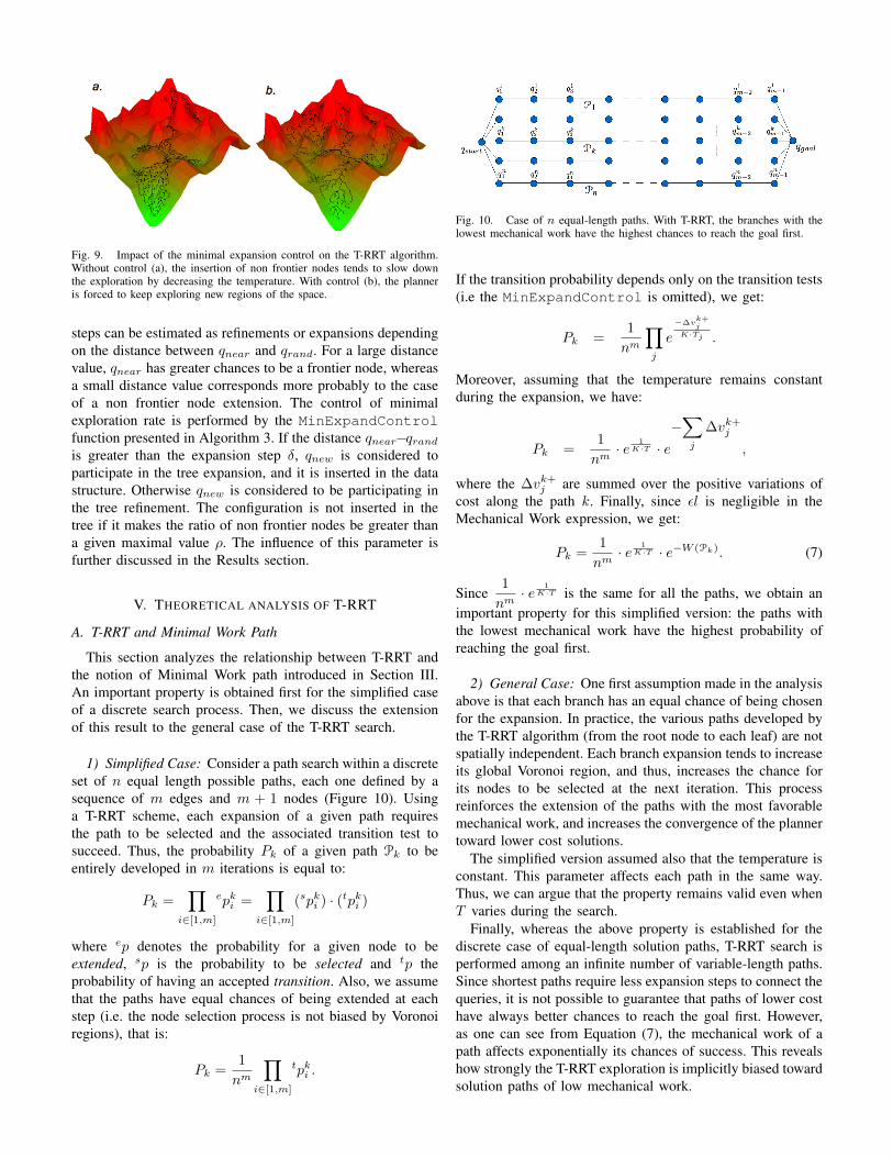
2) Minimal Exploration Rate: The proposed solution is toforce the planner to explore new regions by controlling theratio between exploration and refinement steps. Note that aslong as the tree coverage remains limited compared to thesize of the space, non frontier nodes have a Voronoi regionmuch smaller than the one of frontier nodes. Hence, extension

Fig. 9. Impact of the minimal expansion control on the T-RRT algorithm.Without control (a), the insertion of non frontier nodes tends to slow downthe exploration by decreasing the temperature. With control (b), the planneris forced to keep exploring new regions of the space.

steps can be estimated as refinements or expansions dependingon the distance between qnear and qrand. For a large distancevalue, qnear has greater chances to be a frontier node, whereasa small distance value corresponds more probably to the caseof a non frontier node extension. The control of minimalexploration rate is performed by the MinExpandControlfunction presented in Algorithm 3. If the distance qnear−qrand

is greater than the expansion step δ, qnew is considered toparticipate in the tree expansion, and it is inserted in the datastructure. Otherwise qnew is considered to be participating inthe tree refinement. The configuration is not inserted in thetree if it makes the ratio of non frontier nodes be greater thana given maximal value ρ. The influence of this parameter isfurther discussed in the Results section.

V. THEORETICAL ANALYSIS OF T-RRT

A. T-RRT and Minimal Work Path

This section analyzes the relationship between T-RRT andthe notion of Minimal Work path introduced in Section III.An important property is obtained first for the simplified caseof a discrete search process. Then, we discuss the extensionof this result to the general case of the T-RRT search.

1) Simplified Case: Consider a path search within a discreteset of n equal length possible paths, each one defined by asequence of m edges and m + 1 nodes (Figure 10). Usinga T-RRT scheme, each expansion of a given path requiresthe path to be selected and the associated transition test tosucceed. Thus, the probability Pk of a given path Pk to beentirely developed in m iterations is equal to:

Pk =∏

i∈[1,m]

epki =

∏i∈[1,m]

(spki ) · (tpk

i )

where ep denotes the probability for a given node to beextended, sp is the probability to be selected and tp theprobability of having an accepted transition. Also, we assumethat the paths have equal chances of being extended at eachstep (i.e. the node selection process is not biased by Voronoiregions), that is:

Pk =1nm

∏i∈[1,m]

tpki .

Fig. 10. Case of n equal-length paths. With T-RRT, the branches with thelowest mechanical work have the highest chances to reach the goal first.

If the transition probability depends only on the transition tests(i.e the MinExpandControl is omitted), we get:

Pk =1nm

∏j

e−∆v

k+j

K·Tj .

Moreover, assuming that the temperature remains constantduring the expansion, we have:

Pk =1nm· e 1

K·T · e−∑

j

∆vk+j

,

where the ∆vk+j are summed over the positive variations of

cost along the path k. Finally, since εl is negligible in theMechanical Work expression, we get:

Pk =1nm· e 1

K·T · e−W (Pk). (7)

Since1nm· e 1

K·T is the same for all the paths, we obtain animportant property for this simplified version: the paths withthe lowest mechanical work have the highest probability ofreaching the goal first.

2) General Case: One first assumption made in the analysisabove is that each branch has an equal chance of being chosenfor the expansion. In practice, the various paths developed bythe T-RRT algorithm (from the root node to each leaf) are notspatially independent. Each branch expansion tends to increaseits global Voronoi region, and thus, increases the chance forits nodes to be selected at the next iteration. This processreinforces the extension of the paths with the most favorablemechanical work, and increases the convergence of the plannertoward lower cost solutions.

The simplified version assumed also that the temperature isconstant. This parameter affects each path in the same way.Thus, we can argue that the property remains valid even whenT varies during the search.

Finally, whereas the above property is established for thediscrete case of equal-length solution paths, T-RRT search isperformed among an infinite number of variable-length paths.Since shortest paths require less expansion steps to connect thequeries, it is not possible to guarantee that paths of lower costhave always better chances to reach the goal first. However,as one can see from Equation (7), the mechanical work of apath affects exponentially its chances of success. This revealshow strongly the T-RRT exploration is implicitly biased towardsolution paths of low mechanical work.

B. Probabilistic Completeness

The T-RRT algorithm is a probabilistically complete planner[19]. This property is directly inherited from the probabilisticcompleteness of the RRT planner (see Section 4 of [9]).The only difference is that in the present case, the extensionsteps can be rejected because of the transition tests, evenin the case of a convex, open, n-dimensional subset of ann-dimensional configuration space. However, we argue thatthe success probability of the transitions is always strictlypositive since the cost function takes finite values in thissubset, and thus, the cost variations are bounded. As a result,the planner converges eventually toward an entire coverage ofthe considered subset, and the transition tests affect only theconvergence rate of the algorithm.

VI. EXPERIMENTAL RESULTS

A large set of experiments has been conducted to evaluatethe performance of the planner. First, the general behaviorof the method is presented on various problems. Second, itsperformance is compared to the one of existing methods,highlighting the good quality of the T-RRT solutions. Finally,we investigate the influence of some intrinsic parameterson the overall efficacy of the method. All the algorithmshave been implemented within the path planning softwareMove3D [23]. The performance results summarized in thetables are values averaged over 10 runs.

A. General Performance

A variety of problems are proposed to illustrate thegenerality of the method. The examples vary not only inthe geometrical complexity and the configuration spacedimensionality, but also in the nature of the cost function.Two settings of T-RRT are considered: a greedy version of theplanner referred to as T-RRTg that takes nFailmax = 10, and atempered version, referred to as T-RRTt, with nFailmax = 100.The latter leads to higher quality solution paths, but ismore computationally expensive. We used α = 2 in all theexamples. The results obtained with the Extend version ofthe basic RRT planner are given as references. The tablesalso present comparative results with two existing cost-basedmethods that will be discussed in the next subsection.

The first set of experiments is performed on the two-dimensional cost space of Figure 1. In this example, thesolution paths have to go through a saddle point to link thequery configurations located at two opposite corners of thelandscape. Figure 11 shows snapshots of the exploration treeand the solution path found (Figure 11c), which is close to theoptimal one (Figure 11d). Table II presents the characteristicsof the paths obtained with each planner.4 It provides alsovalues for the MW and IC optimal paths (computed with anA∗ search within a 128×128 grid discretizing the landscape).

The mechanical work of solutions obtained by the differentmethods is reported in the W column. The numbers in

4In the case of RRT, since there is no obstacle in the scene, connectionattempts to the goal are only performed when d(qnew, qgoal) < 15δ toavoid getting a trivial straight-line solution.

Fig. 11. Construction process of the Transition-based RRT planner (a-b).The solution path (c), is close to the optimal one (d) computed from a spacediscretization.

Length Cave Cmax S × 10−3 W TimeRRT 148 22.6 41.2 3.3 45.1 (36.9) 0.1T-RRTg 182 18.2 25 3.9 28.0 (19.7) 0.9T-RRTt 214 17.1 23.2 4.0 23.1 (16.9) 11.0MW path 186 17.9 23.6 3.3 15.9 -IC path 139 18.6 39.6 2.6 41.0 -Thresh. 157-192 17.8-20.9 23.7-32.7 3.3-3.4 27-30 (21-24) 0.3-329

hRRT 155 20.9 33.3 3.2 41.4 (32.9) 0.6

TABLE IICOMPARATIVE RESULTS FOR THE COSTMAP PROBLEM.

parentheses integrate the effect of some local smoothingof the solution path with a simple procedure based on theshortcut algorithm [14]. As one can see from the table,the mechanical work of the reference RRT path is almost3 times higher than for the optimal MW solution, andsmoothing does not successfully get close to the optimalvalue (36.9 vs. 15.9). In comparison, the mechanical workof the path obtained with the tempered version of T-RRTis only 45% higher than for the MW path, and it becomesonly 6% higher than the optimal value after smoothing.Most importantly, the overall shape of the T-RRT solutionis very close to the optimal-MW path and follows the samelow-cost regions. Also, note that the relatively slight lossof path quality of the greedy version is compensated by amuch smaller computing time (0.9s vs. 11.0s). Comparativeresults obtained with other existing costmap planners (Thresh.and hRRT rows in the table) are discussed in Subsection VI-B.

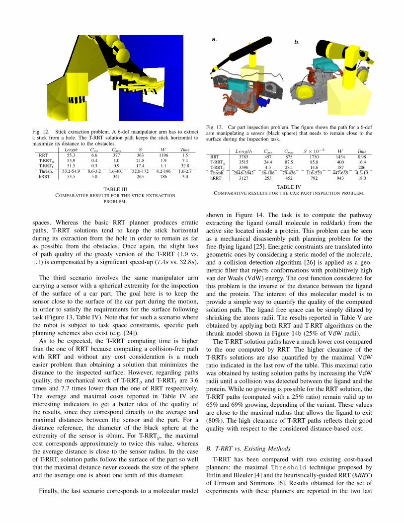
In the next experiment, a 6-dof manipulator arm is carryinga stick in a 3D workspace with obstacles (Figure 12). Here, thegoal is to extract the stick from a hole, while keeping the stickas far as possible from the obstacles. Thus, the cost functionconsidered here is the inverse of the distance between the stickand the obstacles. Results are presented in Table III.

The costs of the T-RRT solution paths are considerablylower than the ones of RRT. This shows the effectiveness ofthe planner for finding low-MW paths in higher-dimensional

Fig. 12. Stick extraction problem. A 6-dof manipulator arm has to extracta stick from a hole. The T-RRT solution path keeps the stick horizontal tomaximize its distance to the obstacles.

Length Cave Cmax S W TimeRRT 55.3 6.6 377 363 1196 1.5T-RRTg 53.9 0.4 1.0 21.8 1.9 7.4T-RRTt 51.5 0.3 0.9 17.4 1.1 32.8Thresh. 53.2-54.9 0.6-3.2 1.6-40.1 32.0-172 4.2-196 1.6-2.7hRRT 53.5 5.0 341 265 786 3.0

TABLE IIICOMPARATIVE RESULTS FOR THE STICK EXTRACTION

PROBLEM.

spaces. Whereas the basic RRT planner produces erraticpaths, T-RRT solutions tend to keep the stick horizontalduring its extraction from the hole in order to remain as faras possible from the obstacles. Once again, the slight lossof path quality of the greedy version of the T-RRT (1.9 vs.1.1) is compensated by a significant speed-up (7.4s vs. 32.8s).

The third scenario involves the same manipulator armcarrying a sensor with a spherical extremity for the inspectionof the surface of a car part. The goal here is to keep thesensor close to the surface of the car part during the motion,in order to satisfy the requirements for the surface followingtask (Figure 13, Table IV). Note that for such a scenario wherethe robot is subject to task space constraints, specific pathplanning schemes also exist (e.g. [24]).

As to be expected, the T-RRT computing time is higherthan the one of RRT because computing a collision-free pathwith RRT and without any cost consideration is a mucheasier problem than obtaining a solution that minimizes thedistance to the inspected surface. However, regarding pathsquality, the mechanical work of T-RRTg and T-RRTt are 3.6times and 7.7 times lower than the one of RRT respectively.The average and maximal costs reported in Table IV areinteresting indicators to get a better idea of the quality ofthe results, since they correspond directly to the average andmaximal distances between the sensor and the part. For adistance reference, the diameter of the black sphere at theextremity of the sensor is 40mm. For T-RRTg , the maximalcost corresponds approximately to twice this value, whereasthe average distance is close to the sensor radius. In the caseof T-RRT, solution paths follow the surface of the part so wellthat the maximal distance never exceeds the size of the sphereand the average one is about one tenth of this diameter.

Finally, the last scenario corresponds to a molecular model

Fig. 13. Car part inspection problem. The figure shows the path for a 6-dofarm manipulating a sensor (black sphere) that needs to remain close to thesurface during the inspection task.

Length Cave Cmax S × 10−3 W TimeRRT 3785 457 875 1730 1434 0.98T-RRTg 3515 24.4 87.5 85.8 400 16.4T-RRTt 3396 4.3 28.1 14.6 187 206Thresh. 2848-3942 36-186 79-436 116-529 447-635 4.3-19hRRT 3127 253 452 792 943 18.0

TABLE IVCOMPARATIVE RESULTS FOR THE CAR PART INSPECTION PROBLEM.

shown in Figure 14. The task is to compute the pathwayextracting the ligand (small molecule in red/dark) from theactive site located inside a protein. This problem can be seenas a mechanical disassembly path planning problem for thefree-flying ligand [25]. Energetic constraints are translated intogeometric ones by considering a steric model of the molecule,and a collision detection algorithm [26] is applied as a geo-metric filter that rejects conformations with prohibitively highvan der Waals (VdW) energy. The cost function considered forthis problem is the inverse of the distance between the ligandand the protein. The interest of this molecular model is toprovide a simple way to quantify the quality of the computedsolution path. The ligand free space can be simply dilated byshrinking the atoms radii. The results reported in Table V areobtained by applying both RRT and T-RRT algorithms on theshrunk model shown in Figure 14b (25% of VdW radii).

The T-RRT solution paths have a much lower cost comparedto the one computed by RRT. The higher clearance of theT-RRTs solutions are also quantified by the maximal VdWratio indicated in the last row of the table. This maximal ratiowas obtained by testing solution paths by increasing the VdWradii until a collision was detected between the ligand and theprotein. While no growing is possible for the RRT solution, theT-RRT paths (computed with a 25% ratio) remain valid up to65% and 69% growing, depending of the variant. These valuesare close to the maximal radius that allows the ligand to exit(80%). The high clearance of T-RRT paths reflects their goodquality with respect to the considered distance-based cost.

B. T-RRT vs. Existing Methods

T-RRT has been compared with two existing cost-basedplanners: the maximal Threshold technique proposed byEttlin and Bleuler [4] and the heuristically-guided RRT (hRRT)of Urmson and Simmons [6]. Results obtained for the set ofexperiments with these planners are reported in the two last

Fig. 14. Two representations of the same ligand-protein “disassembly”problem, with different van der Waals radii: (a) maximal radius and (b) shrunkradius. The goal is to compute paths that maximize the clearance and thusremain valid for large van der Waals radii.

Length Cave Cmax S W Time V dWm

RRT 59 14 2236 826 471 0.7 25T-RRTg 62 0.4 1.0 22 1.25 8.39 65T-RRTt 64 0.3 0.9 22 1.0 426 69Thresh. 58-62 .4-.7 1.1-3.7 25-42 1.4-4.3 4.8-73.5 34-62hRRT 59 8.3 733 490 353 15.2 26

TABLE VCOMPARATIVE RESULTS FOR THE LIGAND-PROTEIN PROBLEM.

rows of Tables II to V. In the case of the threshold method,results are highly sensitive to the threshold growing speed, andthus, reported data correspond to the extremal values obtainedwhen varying this parameter in the range (1-100).

Regarding the mechanical work criterion, results show thatT-RRTt provides significantly better solutions than existingmethods in all tests. Remarkably, T-RRT solutions are alsobetter with respect to the IC criterion in the three more difficultproblems involving a six-dimensional cost space.

The bad overall performance of the hRRT method is dueto the strong bias introduced by the heuristic that steers theexploration toward the goal, resulting in a poor exploratoryability, making it unable to circumvent high-cost regionsand find higher quality paths. Comparatively, the thresholdtechnique can provide solution paths whose quality is close tothe one of T-RRTg , but its performance is highly sensitiveto the parameter that regulates the variation speed of thethreshold. Depending on the value of this parameter, therunning time increases up to 1000 times for the costmapproblem, the mechanical work increases up to 47-fold for thestick extraction problem, and both the running time and themechanical work are notably affected by the threshold speedvalue for the car part inspection problem. Furthermore, thissensitive parameter is problem-dependent and has to be tunedfor each application, whereas T-RRT parameters remain robustto problem changes, as shown in the next subsection.

C. Influence of Intrinsic Parameters

We analyze now the influence of the main parameters ofthe T-RRT algorithm. Experiments are performed on threeproblems that correspond to three different types of costfunctions: the hilly costmap (Figure 11), the stick extractionproblem (Figure 12), and the car part inspection problem(Figure 13). The results are presented in Tables VI and VII.

Hilly costmapTime W

nFailmax nFailmaxα 10 100 1000 10 100 10002 0.9 11.0 121 28.0 23.1 23.410 0.7 7.1 93.4 32.1 26.6 24.450 0.7 7.0 85.5 32.0 28.7 24.8

Stick extractionTime W

nFailmax nFailmaxα 10 100 1000 10 100 10002 7.4 32.8 226 1.9 1.1 1.110 8.2 31.0 218 5.5 2.9 2.450 7.0 29.8 226 3.5 3.3 1.2

Car part inspectionTime W

nFailmax nFailmaxα 10 100 1000 10 100 10002 16.4 206 2012 400 187 16610 14.3 171 1697 439 188 16550 15.9 167 1583 507 212 203

TABLE VIINFLUENCE OF THE α AND nFailmax PARAMETERS.

Bold values are the default settings used in previous tests.

1) Temperature Variation Control: nFailmax and α are thetwo parameters that control the derivative of the temperature,and hence the selectivity of the transition test (as explained inSection IV-B).

Table VI shows that nFailmax is an important parameter thatdetermines the appropriate balance between time performanceand solution path quality. In the costmap problem, whennFailmax is increased by a factor of 10, the running timealso increases 9 to 13-fold. Its influence on the runtimeperformance is less direct on the two manipulator problems(due to the additional cost of collision checking), even thoughthe tendency is the same. Finally, note that higher values ofnFailmax improve path quality, but only up to a point: thequality increases when nFailmax varies from 10 to 100, butremains approximately constant from 100 to 1000.

Regarding the α parameter, results show that it affects onlyslightly the behavior of the algorithm even if higher valuestend to increase the time performance while decreasing thepath quality. Overall, values nFailmax = 100 and α = 2provide the best results for the three examples and are usedas default setting for all tests.

2) Expansion vs. Refinement Control: Table VII presentsresults for various values of the ρ parameter used in theMinExpandControl function to set the maximal ratio ofrefinement nodes.

In the first line of the table, ρ = 1 means that theMinExpandControl function is inactive. The results for the2D hilly costmap highlight the importance of this function, thecomputing time being much higher when ρ = 1. This exampleillustrates the case where the refinement process slows downthe exploration by decreasing the temperature. This effect isless visible in the two other examples where refinement stepsare less likely to happen because of the large size of the space.Results for the other settings (i.e. ρ 6= 1) are quite similar,meaning that ρ does not require to be tuned precisely. In all

Hilly costmap Stick extraction Car part inspectionρ Time W Time W Time W1 420 19.6 30.3 1.1 201 1921/2 16.7 23.7 33.4 1.2 198 2021/10 11.0 23.1 32.8 1.1 206 1871/100 9.7 23.8 32.0 1.2 269 263

TABLE VIIINFLUENCE OF THE ρ PARAMETER.

Fig. 15. A tricky problem for T-RRT. A large low-cost region has to beexplored before deciding to cross the high-cost barrier: useless in (a) or leadingto a better solution (b).

experiments, the default setting ρ = 1/10 appears to be a goodcompromise between computing time and path quality.

VII. EXTENSIONS

A. Bi-directional T-RRT

Similarly to the bi-directional version of the RRT planner[9], a bi-directional T-RRT can be envisaged. However, anaive approach using the same transition test for both treeswould lead to poor quality solutions. It would tend to createpaths with consecutive downhill and uphill cost variations,corresponding to branches expanded from the init-tree andgoal-tree respectively, and may fail to find a more flat so-lution path of lower-MW cost. A better alternative, using theproperty of Subsection III-E2, which states that the MW pathsminimize any cost variations, is to modify transition testsin order to filter both positive and negative cost variationswhen expanding the two trees. This can be achieved easily byreplacing the transition probability pij of Equation (6) by theexpression pij = exp(− |∆c∗ij |

K.T ). Preliminary results show thatthis approach performs well in problems where positive andnegative cost variations for the best cost paths are globally ofthe same amplitude. However, in problems where the profileof the cost between query nodes is asymmetric, it turns out toreject too many configurations during the transition test, whichdegrades the performance. In that case, a method based on amore sophisticated transition test should be designed.

B. Toward a Greedy Anytime T-RRT

In this section, we discuss a possible extension of T-RRTfor performance improvement in tricky situations such as theone illustrated in Figure 15. In this example, the large low-costregion has to be fully explored before determining the needto cross the higher cost barrier (a) or discovering the low-costpassage that yields a better solution (b). In both cases, the

Fig. 16. (a) Initial tree built using a greedy T-RRT version. (b) The additionof cycles (in red) leads to higher quality paths.

greedy T-RRTg version may rapidly cross the barrier, and thusspeed-up the computation compared to the tempered T-RRTt.However, it may miss the preferred detour path in problem (b),for which a longer exploration is needed to find the passage.To keep the performance of an aggressive exploration whileavoiding this issue, we propose to combine the greedy versionof the planner with a cycle addition mechanism. The idea isto create cycles in the tree when good paths initially missedduring the search are discovered afterwards. The idea has beentested using the technique of [27] for cycle addition, leadingto early results. Figure 16 shows an initial tree built using agreedy version of T-RRT that goes through a medium costregion (circled in blue on Figure 16a) that could have beenavoided. The addition of cycles provides alternative paths andyields higher quality solutions (Figure 16b).

VIII. CONCLUSION AND FUTURE WORK

We have presented a sampling-based algorithm to computepaths in problems involving high-dimensional cost spaces.The proposed method combines the exploratory strength ofRRTs, with the efficiency of stochastic optimization methods.It integrates an adaptive mechanism that helps to ensure a goodperformance for a large set of problems.

The notion of Minimal Work path has been proposed toquantify the quality of solution paths. By design, the proposedT-RRT algorithm computes paths that tend to satisfy such aquality property. A large set of experiments were performedto show the efficacy of the T-RRT planner.

Experimental results have shown that the planner is generalenough to be applied, at least, to 6-dimensional spaces con-strained by obstacles. Future work concerns the applicationof T-RRT to new classes of problems such as the integrationof human-robot interaction constraints within path planning orthe exploration of energy landscapes in computational biologyproblems. Extensions discussed in the previous section alsoneed to be further explored for performance improvement.Furthermore, another direction is to incorporate in the plannerother methods inspired by Monte Carlo optimization tech-niques, such as stochastic tunneling [28] or parallel tempering[29]. Finally, it would be interesting to test our approach onbenchmark problems of the stochastic optimization commu-nity, since T-RRT could be used as a generic optimizationtool and, in principle, applied to any metric cost space.

IX. ACKNOWLEDGMENTS

This work has been partially supported by the the FrenchNational Research Agency under project “GlucoDesign”, bythe European Community under FP7-ICT project 216239“DEXMART”, and by the Spanish Ministry of Science andInnovation under project DPI2007-60858. Leonard Jaillet wassupported by CSIC under JAE-Doc fellowship.

REFERENCES

[1] H. Choset, K. Lynch, S. Hutchinson, G. Kantor, W. Burgard, L. Kavraki,and S. Thrun, Principles of Robot Motion: Theory, Algorithms, andImplementations. Cambridge: MIT Press, 2005.

[2] S. LaValle, Planning Algorithms. New York: Cambridge UniversityPress, 2006.

[3] A. Stentz, “Optimal and efficient path planning for partially-knownenvironments,” Proc. IEEE Int. Conf. on Robotics and Automation, pp.3310–3317, 1994.

[4] A. Ettlin and H. Bleuler, “Rough-terrain robot motion planning basedon obstacleness,” Proc. Int. Conf. on Control, Automation, Robotics andVision, pp. 1–6, 2006.

[5] ——, “Randomised rough-terrain robot motion planning,” Proc.IEEE/RSJ Int. Conf. on Intelligent Robots and Systems, pp. 5798–5803,2006.

[6] C. Urmson and R. Simmons, “Approaches for heuristically biasing RRTgrowth,” Proc. IEEE/RSJ Int. Conf. on Intelligent Robots and Systems,pp. 1178–1183, 2003.

[7] D. Ferguson and A. Stentz, “Anytime RRTs,” Proc. IEEE/RSJ Int. Conf.on Intelligent Robots and Systems, pp. 5369 – 5375, 2006.

[8] R. Diankov and J. Kuffner, “Randomized statistical path planning,” Proc.IEEE/RSJ Int. Conf. on Intelligent Robots and Systems, pp. 1–6, 2007.

[9] J. Kuffner and S. LaValle, “RRT-connect: An efficient approach tosingle-query path planning,” Proc. IEEE Int. Conf. on Robotics andAutomation, pp. 995–1001, 2000.

[10] J. Lee, C. Pippin, and T. Balch, “Cost based planning with RRT inoutdoor environments,” Proc. IEEE/RSJ Int. Conf. on Intelligent Robotsand Systems, pp. 684–689, 2008.

[11] L. Jaillet, J. Cortes, and T. Simeon, “Transition-based RRT for pathplanning in continuous cost spaces,” Proc. IEEE/RSJ Int. Conf. onIntelligent Robots and Systems, pp. 2145–2150, 2008.

[12] J.-C. Latombe, Robot Motion Planning. Boston: Kluwer AcademicPublishers, 1991.

[13] J. Barraquand and J.-C. Latombe, “A Monte-Carlo algorithm for pathplanning with many degrees of freedom,” Proc. IEEE Int. Conf. onRobotics and Automation, pp. 1712–1717, 1990.

[14] S. Sekhavat, P. Svestka, and M. Overmars, “Multi-level path planning fornonholonomic robots using semi-holonomic subsystems,” InternationalJournal of Robotics Research, vol. 17(8), pp. 840–857, 1998.

[15] R. Geraerts and M. H. Overmars, “Creating high-quality paths formotion planning,” International Journal of Robotics Research, vol. 26,pp. 845–863, 2007.

[16] J. Spall, Introduction to Stochastic Search and Optimization. New York:Wiley, 2003.

[17] S. Kirkpatrick, C. Gelatt, and M. Vecchi, “Optimization by simulatedannealing,” Science, vol. 220, pp. 671–680, 1983.

[18] M. Apaydin, A. Singh, D. Brutlag, and J.-C. Latombe, “Captur-ing molecular energy landscapes with probabilistic conformationalroadmaps,” Proc. IEEE Int. Conf. on Robotics and Automation, pp. 932–939, 2001.

[19] L. Kavraki, P. Svestka, J.-C. Latombe, and M. Overmars, “Probabilisticroadmaps for path planning in high-dimensional configuration spaces,”IEEE Transactions on Robotics and Automation, vol. 12(4), pp. 566–580, 1996.

[20] S. LaValle, “Rapidly-Exploring Random Trees: A New Tool for PathPlanning,” 1998, TR 98-11, CS Dept., Iowa State University.

[21] A. Yershova, L. Jaillet, T. Simeon, and S. LaValle, “Dynamic-domainRRTs: Efficient exploration by controlling the sampling domain,” Proc.IEEE Int. Conf. on Robotics and Automation, pp. 3867–3872, 2005.

[22] L. Jaillet, A. Yershova, S. LaValle, and T. Simeon, “Adaptive tuning ofthe sampling domain for dynamic-domain RRTs,” Proc. IEEE/RSJ Int.Conf. on Intelligent Robots and Systems, pp. 4086–4091, 2005.

[23] T. Simeon, J.-P. Laumond, and F. Lamiraux, “Move3D: A genericplatform for path planning,” Proc. IEEE Int. Symp. on Assembly & TaskPlanning, pp. 25–30, 2001.

[24] M. Stilman, “Task constrained motion planning in robot joint space,”Proc. IEEE/RSJ Int. Conf. on Intelligent Robots and Systems, pp. 3074–3081, 2007.

[25] J. Cortes, L. Jaillet, and T. Simeon, “Disassembly path planning forcomplex articulated objects,” IEEE Transactions on Robotics and Au-tomation, pp. 475–481, 2008.

[26] V. Ruiz de Angulo, J. Cortes, and T. Simeon, “BioCD: An efficientalgorithm for self-collision and distance computation between highlyarticulated molecular models,” in Robotics: Science and Systems, S. T.snd G. Sukhatme, S. Schaal, and O. Brock, Eds. Cambridge: MITPress, 2005, pp. 6–11.

[27] D. Nieuwenhuisen and M. Overmars, “Useful cycles in probabilisticroadmap graphs,” Proc. IEEE Int. Conf. on Robotics and Automation,pp. 446– 452, 2004.

[28] K. Hamacher and W. Wenzel, “Scaling behavior of stochastic minimiza-tion algorithms in a perfect funnel landscape,” Phys. Rev. E, vol. 59,no. 1, pp. 938–941, Jan 1999.

[29] D. J. Earl and M. W. Deem, “Parallel tempering: Theory, applications,and new perspectives,” Physical Chemistry Chemical Physics, vol. 7, pp.3910–3916, 2005.

Leonard Jaillet received the Eng. degree in me-chanical engineering from the Institut Superieurde Mecanique de Paris and the Ph.D. degree inrobotics from the University of Toulouse, France,in 2001 and 2005, respectively. Since 2008, he isPostdoctoral Fellow at the Institut de Robotica iInformatica Industrial, Spanish National ResearchConcil, Barcelona. His research interest includesmotion planning for complex robotic systems andmolecular simulations for structural biology.

Juan Cortes received the engineering degree in con-trol and robotics from the Universidad de Zaragoza(Spain) in 2000. In 2003, he received the Ph.D. de-gree in robotics from the Institut National Polytech-nique de Toulouse (France). From 2004, he is CNRSresearcher at LAAS (Toulouse, France). His researchinterest is focused around the development of algo-rithms for computing and analyzing the motion ofcomplex systems in robotics and structural biology.He co-chairs the IEEE-RAS TC on Algorithms forPlanning and Control of Robot Motion.

Thierry Simeon received the engineering degreein computer science from INSA, Toulouse, Franceand the Ph.D degree in robotics from the Universityof Toulouse, in 1985 and 1989, respectively. Since1990, he has been with LAAS-CNRS, Toulouse,France. His primary research interest includes robotmotion planning and applications to structural bioin-formatics. He is co-author of more than 100 papersand was a co-founder of the LAAS spin-off KineoCAM. He is currently an Associate Editor of theIEEE Transactions on Robotics.