Sampling Theorem Notes Class: Digital Communications Dentato 2012 Sampling Theorem We will show that a band limited signal () || can be reconstructed exactly from its discrete time samples. Recall: That a time sampled signal is like taking a snap shot or picture of signal periodically. Consider the signal () as follows Figure 1: Sampled Signal Multiplying () by a pulse train (), which is periodic with period , we get the signal ̅() which is a sampled version of (). We find that ̅() () () ∑ ( )( )
Transcript
Sampling Theorem Notes
Class: Digital Communications Dentato 2012
Sampling Theorem
We will show that a band limited signal
( ) | |
can be reconstructed exactly from its discrete time samples.
Recall: That a time sampled signal is like taking a snap shot or picture of signal periodically.
Consider the signal ( ) as follows
Figure 1: Sampled Signal
Multiplying ( ) by a pulse train ( ), which is periodic with period , we get the signal ( ) which
is a sampled version of ( ). We find that
( ) ( ) ( ) ∑ ( ) ( )
Sampling Theorem Notes
Class: Digital Communications Dentato 2012
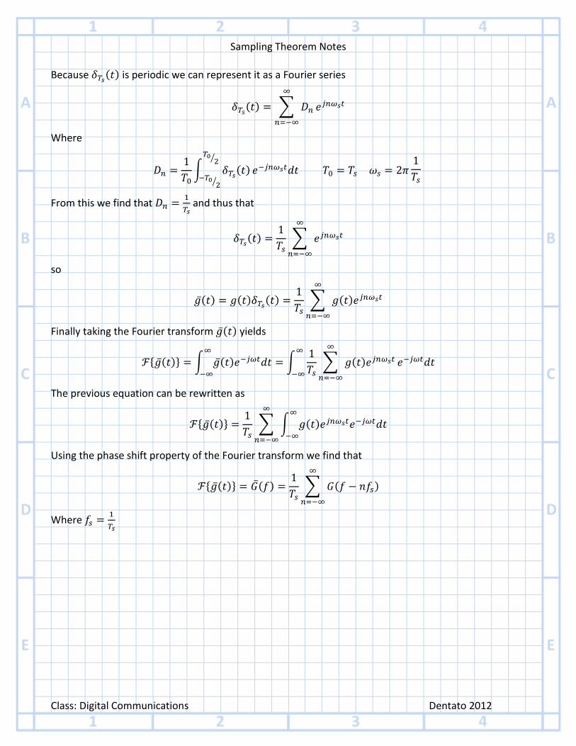
Because ( ) is periodic we can represent it as a Fourier series
( ) ∑
Where
∫ ( )
⁄
⁄
From this we find that
and thus that
( )
∑
so
( ) ( ) ( )
∑ ( )
Finally taking the Fourier transform ( ) yields
{ ( )} ∫ ( )
∫
∑ ( )
The previous equation can be rewritten as
{ ( )}
∑ ∫ ( )
Using the phase shift property of the Fourier transform we find that
{ ( )} ( )
∑ ( )
Where
Sampling Theorem Notes
Class: Digital Communications Dentato 2012
Figure 2: Spectrum of a Sampled Signal ( )
The interesting result of this exercise is that we find the sampled signal ( ) has a spectrum that contains copies of the transform ( ) centered at every . To recover this signal ( ) in entirety we simply have to place a low-pass filter of bandwidth centered at . Notice that we could also place a band-pass filter of bandwidth around any to get a modulated version of the signal where the carrier would be .
What we also need to take note of is that if is less than the signal spectrum will have the copies overlapping or aliasing each other. In order to have no overlap we must
have or
which is referred to as the Nyquist rate.
For a look at an aliased spectrum take a look at Figure 3.
Sampling Theorem Notes
Class: Digital Communications Dentato 2012
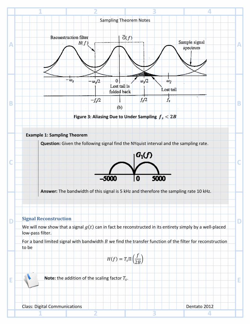
Figure 3: Aliasing Due to Under Sampling
Signal Reconstruction
We will now show that a signal ( ) can in fact be reconstructed in its entirety simply by a well-placed low-pass filter.
For a band limited signal with bandwidth we find the transfer function of the filter for reconstruction to be
( ) (
)
Note: the addition of the scaling factor .
Example 1: Sampling Theorem
Question: Given the following signal find the NYquist interval and the sampling rate.
Answer: The bandwidth of this signal is 5 kHz and therefore the sampling rate 10 kHz.
Sampling Theorem Notes
Class: Digital Communications Dentato 2012
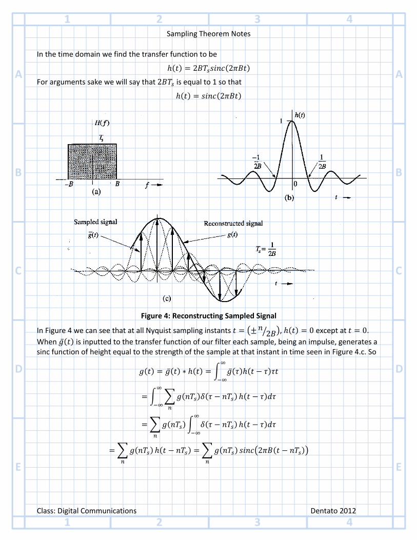
In the time domain we find the transfer function to be
( ) ( )
For arguments sake we will say that is equal to 1 so that
( ) ( )
Figure 4: Reconstructing Sampled Signal
In Figure 4 we can see that at all Nyquist sampling instants ( ⁄ ), ( ) except at .
When ( ) is inputted to the transfer function of our filter each sample, being an impulse, generates a sinc function of height equal to the strength of the sample at that instant in time seen in Figure 4.c. So
( ) ( ) ( ) ∫ ( ) ( )
∫ ∑ ( ) ( )
( )
∑ ( )
∫ ( )
( )
∑ ( )
( ) ∑ ( )
( ( ))
Sampling Theorem Notes
Class: Digital Communications Dentato 2012
Recall: The integral of a delta function is ∫ ( ) ( )
( )
We also find that
( ) ∑ ( )
( ( ))
∑ ( )
( ( ))
What we showed above is that the reconstruction of the signal ( ) from ( ) is an interpolation formula which yields ( ) as a weight sum of all the samples.
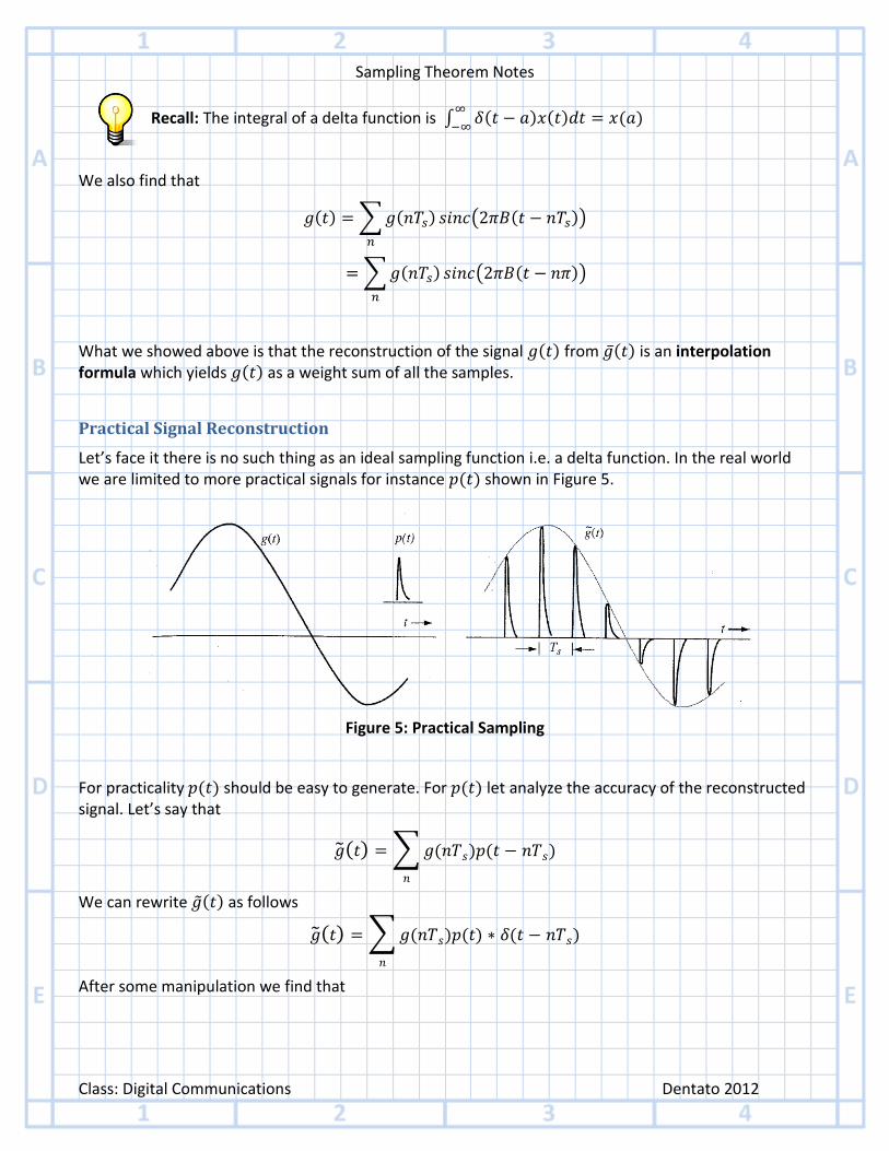
Practical Signal Reconstruction
Let’s face it there is no such thing as an ideal sampling function i.e. a delta function. In the real world we are limited to more practical signals for instance ( ) shown in Figure 5.
Figure 5: Practical Sampling
For practicality ( ) should be easy to generate. For ( ) let analyze the accuracy of the reconstructed signal. Let’s say that
( ) ∑ ( ) ( )
We can rewrite ( ) as follows
( ) ∑ ( ) ( ) ( )
After some manipulation we find that
Sampling Theorem Notes
Class: Digital Communications Dentato 2012
( ) ( ) ∑ ( ) ( )
The Fourier transform yields
( ) ( ) ( ) ( )
∑ (
)
This is an interesting result because what it says is that rather than having to walk through a barrage of mathematically equations to determine how to reconstruct ( ), we can simply find a transfer function that will essentially undue the results of sampling a signal with a non-ideal sampling function in this case ( ). We will refer to this transfer function as an equalizer. The end result of apply an equalizer is that afterwards the signal simply becomes ( ).
Recall: We showed earlier that ( ) can be extracted by a simple, well placed, low-pass filter.
( ) (
)
( ) ∑ ( ) (
)
( ) ( )
( ) {
( ) ⁄ | |
| | ( )⁄
| | ( )⁄
Example 2: Non-Ideal Sampling
Let’s consider a simple interpolating pulse generator that generates short (zero-order hold) pulses.
We have
For reconstruction we first have
The transfer function of ( ) is
As a result the equalizer must satisfy
Sampling Theorem Notes
Class: Digital Communications Dentato 2012
Quantization
Figure 6: Quantization
What it means to quantize a signal is to limit the possible values that a signal can take on. For instants, a discrete signal can have any range of amplitudes at a discrete time interval. Well in order to represent such a signal digitally, let’s say, we would have to have an infinite amount of bits to do this. Since no computer exist that can handle an infinite bit data sample we quantize the data to fit within a range that we are comfortable with and fits our requirements for the system.
L =L
eve
ls
Sampling Theorem Notes
Class: Digital Communications Dentato 2012
It turns out that we will not change the signal per se, rather we will increase the noise level of the signal.
Previously we demonstrated the interpolation formula
( ) ∑ ( ) ( )
If we consider the ( ) as to be the sample of the message signal ( ) the interpolation is as follows
( )
Example 3: Quantization
We have a radio receiver that will never receive a signal greater than (p = peak refer to
Figure 6). Well at this point we can say to ourselves we do not need to have a signal greater that so all signals will only take on values between . Our accuracy or resolution of
the signal depends on L. For larger values of L we will have move voltage resolution. Let’s say we later find out that our voltage accuracy is we can use an L value of 8 where
If we decided to represent this signal digitally we could say we need or 3 bits and now any incoming signal will take on values between and in steps. Another way to say it is that we can only detect a change in the incoming signals voltage. For an 8 bit binary number we have
Binary 000 001 010 011 100 101 110 111
Decimal 0 1 2 3 4 5 6 7
x0.25V 0 0.25 0.50 0.75 1 1.25 1.50 1.75
-1V -1.00 -0.75 -0.50 -0.25 0.00 0.25 0.50 0.75
But if we quantize the signal doesn’t that change the
signal all together?
Sampling Theorem Notes
Class: Digital Communications Dentato 2012
( ) ∑ ( ) ( )
And for the quantized signal let ( ) be the sample of the signal ( ) then
( ) ∑ ( ) ( )
The distortion component ( ) is then
( ) ∑[ ( ) ( )] ( )
∑ ( ) ( )
The signal ( ) is an undesired and acts as noise which leads to the term quantization noise.
To calculate the power of the quantization noise we do the following
( )
∫ ( )
∫ [∑ ( ) ( )
]
Where ( ) denotes the mean square power. Since the a since function
( ) and ( ) are orthogonal ever where but at we find that
( )
∫∑ ( )
( )
∑ ( )
∫ ( )
From the orthogonality relationship it follows that
( )
∑ ( )
Assuming that the error is equally likely be anywhere between (
) we will find that the
quantization noise is
( )
Since the power of the message signal
( )
Sampling Theorem Notes
Class: Digital Communications Dentato 2012
It is clear that the Signal to Quantization Noise Ratio (SQNR) is
( )
Quantization will be in addition to whatever other noise is present in the system.
Some Applications of the Sampling Theorem
Sampling theorem is important because it allows a continuous signal to be sampled and then transmitted as a discrete number rather than a continuous time signal. Processing a continuous signal is then equivalent to processing a discrete signal. Discrete values can be transmitted by multiple variations of a pulse train.
Pulse Amplitude Modulation (PAM)
( )
( )
( )
(
( )
)
( ) ( )
( ) ( )
( )
Example 4: Power of Quantized Signal
Question: If an audio signal has average power of 0.1W and a peak voltage of 1V. What is the resulting SQNR if L = 50,000 levels.
Answer: When you see average power think mean square power or ( ) unless otherwise noted. With this we have
Where a the decibel value is calculated as
Question: How many bits would be required to represent one sample from this audio signal?
Answer:
Well there is no such thing as 15.61 bits so we must round up to 16 bits in order to represent the largest possible quantization of the signal.
Sampling Theorem Notes
Class: Digital Communications Dentato 2012
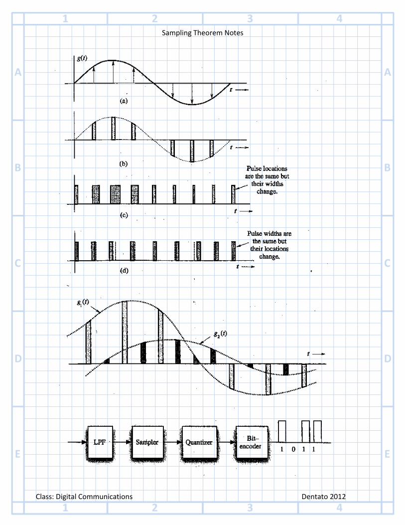
Pulse Width Modulation (PWM)
Pulse Position Modulation (PPM)
Pulse Code Modulation (PCM)
Although the method of creating and representing a quantized signal via a manipulated pulse train may
vary the data being transmitted does not. See the image below.
Sampling Theorem Notes
Class: Digital Communications Dentato 2012
Sampling Theorem Notes
Class: Digital Communications Dentato 2012
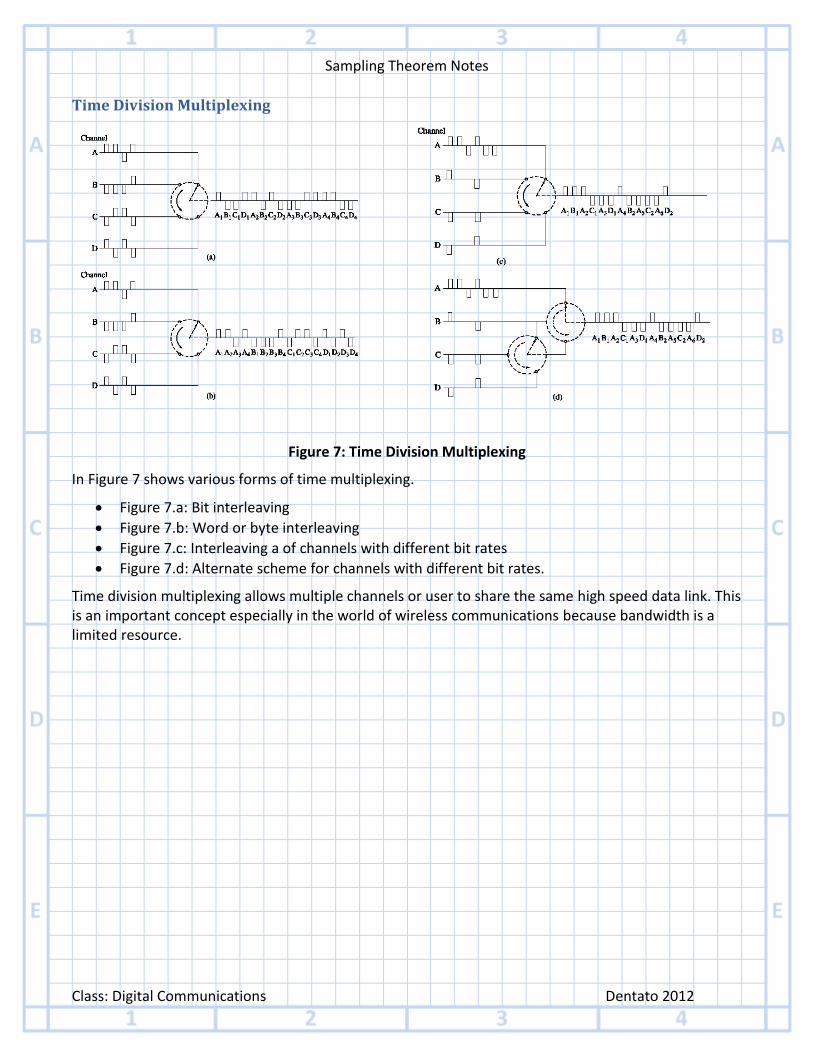
Time Division Multiplexing
Figure 7: Time Division Multiplexing
In Figure 7 shows various forms of time multiplexing.
Figure 7.a: Bit interleaving
Figure 7.b: Word or byte interleaving
Figure 7.c: Interleaving a of channels with different bit rates
Figure 7.d: Alternate scheme for channels with different bit rates.
Time division multiplexing allows multiple channels or user to share the same high speed data link. This is an important concept especially in the world of wireless communications because bandwidth is a limited resource.
Sampling Theorem Notes
Class: Digital Communications Dentato 2012
Example 5: Data Transmission and Time Multiplexing
Question: A wireless communication provider would like to time divide voice data from as many users as possible in order to transmit it over a new wireless link that has a bandwidth of 20MHz. In order to minimize data errors, engineers decide that they must sample data on the link at 20% above the Nyquist rate. If we can only transmit 2bits/s/Hz
(a) What is the maximum sampling rate that can be achieved for this new wireless channel?
(b) How many bits/s can be transmitted on this channel? (c) If each user will be transmitting data at 500Kbs/s how many users can this channel
serve?
Answer: The Nyquist sampling criteria says that we must sample at
. In this case
we have a channel that has so , but we must also account for the 20% over sampling that engineering has advised us of thus ( ) which means that our max bandwidth is really only . Since we can only
transmit 2bits/s/Hz we find the maximum bitrate of the channel is
⁄ .
If each user transmits 500Kbs/s we find that the channel can service 8 users.