105
| Date post: | 09-Mar-2016 |
| Category: |
Documents |
| Upload: | vince-murphy |
| View: | 212 times |
| Download: | 0 times |

2
Acknowledgements We wish to thank the Species at Risk Stewardship Program for funding this work along with the substantial direct and in-kind support from the main partner agencies including the Ontario Ministry of Natural Resources (OMNR) Kemptville and Peterborough offices, Eastern Ontario Model Forest (EOMF), Environment Canada, Raisin River Conservation Authority, Rideau Valley Conservation Authority, South Nation Conservation Authority, City of Ottawa, Nature Conservancy of Canada. We are specifically indebted to the project leaders Linda Touzin and Gary Nielson of OMNR and the members of the steering committee who provided invaluable guidance and feedback throughout the project. Project Steering Committee Members: Linda Touzin, OMNR Gary Nielsen, OMNR Allan Bibby, OMNR Gary Bell, Nature Conservancy of Canada Kerry Coleman, OMNR Kevin Cover, City of Ottawa Christie Curley, OMNR Martin Czarski, OMNR Glenn Desy, OMNR Rudy Dyck, Rideau Valley CA Dorothy Hamilton, Raisin River CA Elizabeth Holmes, EOMF Kathy Lindsay, Environment Canada Rick Moll, Statistics Canada Erin Neave, Environment Canada Cathy Nielsen, Environment Canada Danijela Puric-Mladenovic, OMNR Slivia Strobl, OMNR Julia Sutton, South Nation CA

3
Table of Contents Page #
1.0 Introduction 5 2.0 Methods 6 2.1 Study Area 6 2.2 Thematic Classification 7 2.2.1 Forest Classes 10 2.2.2 Agricultural Classes 10 2.2.3 Wetland Classes 10 2.2.4 Developed and Transportation Classes 10 2.3 Input Data Preparation 10 2.3.1 FRI Compilation 12 2.3.1.1 Consistent Attributes. 13 2.3.1.2 Dissolving Boundaries. 14 2.3.1.3 Parsing Species Strings 15 2.3.1.4 Manually Editing Unclassified Areas 16 2.3.2 Agricultural Classification Data 16 2.3.2.1 AAFC Crop Data 17 2.3.2.2 OLCD Agricultural Data 18 2.3.3 Wetlands 19 2.3.4 Urban and Developed Data 21 2.3.5 Roads, Railways, and Transmission Lines 22 2.3.6 Hedgerows 22 2.3.7 County Soils Data 22 2.3.8 FRI Soil Moisture 23 2.3.8.1 CART Sample Dataset 23 2.3.8.2 CART Algorithm 24 2.3.8.1 CART Analysis Runs 26 2.3.9 Terrain 27 2.3.9.1 Relative Slope Position (RSP) 27 2.3.9.2 Terrain Complexity Index (COMP) 28 2.3.9.3 Topographic Convergence Index (TCI) 28 2.3.9.4 Topographic Relative Moisture Index (TRMI) 30 2.3.10 Combining Terrain, Soils, and FRI Data for Ecosite Prediction 30 2.3.11 Composite Scores for Terrain and Soils Attributes 31 2.3.12 RVCA Reforestation Sites 32 2.3.13 NRVIS Water Layer 32 2.4 Ecosite Assignment Rules 32 2.4.1 Summary Attributes 32 2.4.1.1 Forest Versus Non-forest 33 2.4.1.2 Broad Forest Type 33 2.4.1.3 Plantations 33 2.4.1.4 Swamps 34 2.4.1.5 Dry / Fresh Sites Versus Fresh / Moist Sites 34 2.4.1.6 Organic Dominated Sites 34 2.4.2 Assigning Non-forest and Non-swamp Classes 35 2.4.3 Assigning Forest and Swamp Ecosites 35 2.4.4 Cultural Ecosites 35 2.5 Temporal Updating Using SOLRIS Data 36 2.5.1 FRI Forest, SOLRIS Non-forest 38 2.5.1.1 SOLRIS V1-2 Identification 38 2.5.1.2 Young Forest and Plantations 38 2.5.1.3 Rural Developed Areas (Farmsteads) 39 2.5.1.4 Forest Adjacent to Agriculture 39 2.5.1.5 Older Plantations 39 2.5.1.6 Isolated Forest 40

4
2.5.2 SOLRIS Forest, FRI Non-forest 40 2.6 Final Land Cover Compilation 41 2.6.1 Controlling Spatial Precedence 42 2.6.2 Spatial Filtering 43 2.6.2.1 Identifying Large Slivers and Home / Farmsteads 44 2.6.3 Final Comparison with SOLRIS Version 1-2 45 2.6.4 Seamless Compilation Across EOMF 45 2.6.5 Vector Layers 46 2.6.6 Linkages to Original Input Data 47 2.6.7 Linkages to Data Source Names and Dates 48 2.7 Updating Layer in the Future 48 3.0 Habitat Models and Mapping 51 4.0 Final Deliverables 56 4.1 Key Benefits and Potential Uses of the Deliverables 56 4.2 Limitations of the SAR Layer 56 4.3 Planned Combination of SAR Layer with Predicted Vegetation Mapping 57 5.0 References 58 Appendix I Ecosite Assignment Rules 60 Appendix II Spatial Database Description 65 Appendix III Protocol for Developing Species at Risk Habitat Suitability Models 75

5
1.0 Introduction As part of the Species at Risk Stewardship Fund project to predict habitat for Eastern Ontario Species at Risk (SAR), Spatialworks was contracted to develop a digital layer of Ecological Land Classification (ELC) information and map a series of habitat models developed by project partners. Development of the spatial input layers and the final Ecosite layer was completed following a methodology developed by Spatialworks for the National Agri-Environmental Standards Initiative (NAESI) biodiversity theme project for the counties of Stormont, Dundas and Glengarry. We refer the reader to an earlier comprehensive report on this methodology for many of the background details of the approach taken in the NAESI project (Neave et al. 2008). While many technical steps were similar to the NAESI project, significant modifications and enhancements were made to the methodology to accommodate the much larger study area, differing data sources and mapping requirements for the SAR project. Many of the descriptions here are similar to the NAESI documentation with appropriate changes made to reflect the new methods and details. While this results in some duplication it will prevent the reader from having to refer simultaneously to two documents. Similar to the NAESI project, the new data layer created represents an important improvement in spatial information for SAR and other natural resources mapping. Combining fine-scale vegetation mapping with the surrounding matrix of agricultural, urban and developed and transportation land uses in a single layer is critical to provide an integrated landscape context to SAR and other mapping requirements. The following report will document:
- Technical details adapted from the NAESI methodology to accommodate SAR project goals, data availability, and ecological characteristics of the wider Eastern Ontario Model Forest (EOMF) study area;
- The final deliverables and how these data will be most useful in SAR mapping and other land use and habitat evaluation decisions in the future;
- Limitations of the final data layer; - Examples of how the data layer can be used to map SAR models developed by others
under this project.

6
2.0 Methods Many of the technical methods were applied directly from the NAESI mapping project, however, many changes were required to:
- Accommodate differences in input datasets within the larger study area; - Incorporate new and more detailed information on wetlands available since the
completion of the NAESI mapping project; - Provide explicit links in the final data layer to important source datasets (Forest
Resources Inventory, Evaluated Wetlands data) required for SAR mapping and other future uses;
- Process the data by section and recompile as a single layer to avoid physical hardware and software limits for the large study area.
The following sections outline the broad technical steps used to complete the mapping process and how it can be modified and expanded in the future to facilitate updating as new and updated data becomes available. Detailed technical documentation of exact GIS steps/commands and specific metadata will be provided to custodians and users as the data is distributed. 2.1 Study Area The study area and extent of the final land cover layer is approximately 1.5 million hectares and comprises the entire EOMF, excluding some of the islands in the St. Lawrence River where basic input data was not available (Figure 1). Final land cover information was compiled for the entire study area by combining data from a set of administrative units for which key input datasets were originally derived (e.g. FRI, Ottawa land use etc.). While the EOMF-wide dataset will be useful when this context is required, in many cases, subsets of the data will be used for practical purposes such as limiting processing / drawing times for analyses and mapping. Following consultation with the steering committee, subsets based on the original administrative units as well as Conservation Authority (CA) boundaries were created. The original administrative units included:
- Lanark County (Lanark) - City of Ottawa (Ottawa) - United Counties of Prescott and Russell (Prescott) - United Counties of Stormont, Dundas, and Glengarry (SD&G) - United Counties of Leeds and Grenville (Leeds)
CA datasets were created to include the CA boundary plus an addition 5 km of data where possible to ensure the data can be partitioned by the most recent boundaries and to provide context adjacent to the CA boundary. Data subsets were made for the portions of five CA’s within the study area including:
- Cataraqui Region Conservation Authority (CRCA) - Mississippi Valley Conservation Authority (MVCA)

7
- Raisin Region Conservation Authority (RRCA) - Rideau Valley Conservation Authority (RVCA) - South Nation Conservation Authority (SNCA)
Figure 1. Project study area. 2.2 Thematic Classification A thematic classification for the final land cover layer was developed based on the NAESI project. Changes were made to accommodate data availability in the larger study area including areas with more detailed information available (e.g. wetlands) as well as areas where data is less detailed or not available (e.g. agricultural classifications). The goal, as in the NAESI project, was to provide as much detail as could be mapped with the given data and nested classes to allow aggregation of the finest classes when this detail is not required for species habitat or other uses. For example, many habitat models recognize that a species will use similar cover types in the same way, allowing these classes to be aggregated to improve processing efficiency and interpretation (e.g. forest ecosites aggregated to deciduous, coniferous, mixed if there is no preference within these categories).

8
The final thematic classification represents the highest level of detail that the project team was confident mapping with the given input data (Table 1). The classification provides a hierarchy of classes to accommodate differences in thematic detail currently available from the input data that can be expanded as new information becomes available. For example, certain areas have no information to differentiate agricultural types. These areas remain mapped as Agriculture (Class 69) but can be subdivided in the future, as new information is available. Table 1. Final thematic classification for the SAR mapping project.
Class # Class Name 101 Forest 10 Ecosite FOC1 - Dry-Fresh Pine Coniferous Forest 11 Ecosite FOC2 - Dry-Fresh Cedar Coniferous Forest 12 Ecosite FOC3 - Fresh-Moist Hemlock Coniferous Forest 13 Ecosite FOC4 - Fresh-Moist White Cedar Coniferous Forest 14 Ecosite FOM1 - Dry Oak-Pine Mixed Forest 15 Ecosite FOM2 - Dry-Fresh White Pine-Maple-Oak Mixed Forest 16 Ecosite FOM3 - Dry-Fresh Hardwood-Hemlock Mixed Forest 17 Ecosite FOM4 - Dry-Fresh White Cedar Mixed Forest 18 Ecosite FOM5 - Dry-Fresh White Birch-Poplar-Conifer Mixed Forest 19 Ecosite FOM6 - Fresh-Moist Hemlock Mixed Forest 20 Ecosite FOM7 - Fresh-Moist White Cedar-Hardwood Mixed Forest 21 Ecosite FOM8 - Fresh-Moist Poplar-White Birch Mixed Forest 22 Ecosite FOD1 - Dry-Fresh Oak Deciduous Forest 23 Ecosite FOD2 - Dry-Fresh Oak-Maple-Hickory Deciduous Forest 24 Ecosite FOD3 - Dry-Fresh Poplar-White Birch Deciduous Forest 25 Ecosite FOD4 - Dry-Fresh Deciduous Forest 26 Ecosite FOD5 - Dry-Fresh Sugar Maple Deciduous Forest 27 Ecosite FOD6 - Fresh-Moist Sugar Maple Deciduous Forest 28 Ecosite FOD7 - Fresh-Moist Lowland Deciduous Forest 29 Ecosite FOD8 - Fresh-Moist Poplar-Sassafras Deciduous Forest 30 Swamps 31 Comm. Series SWC - Coniferous Swamp 32 Ecosite SWC1 - White Cedar Mineral Coniferous Swamp 33 Ecosite SWC2 - White Pine-Hemlock Mineral Coniferous Swamp 34 Ecosite SWC3 - White Cedar Organic Coniferous Swamp 35 Ecosite SWC4 - Tamarack-Black Spruce Organic Coniferous Swamp 36 Comm. Series SWM - Mixed Swamp 37 Ecosite SWM1 - White Cedar Mineral Mixed Swamp 38 Ecosite SWM2 - Maple Mineral Mixed Swamp 39 Ecosite SWM3 - Birch-Poplar Mineral Mixed Swamp 40 Ecosite SWM4 - White Cedar Organic Mixed Swamp 41 Ecosite SWM5 - Maple Organic Mixed Swamp 42 Ecosite SWM6 - Birch-Poplar Organic Mixed Swamp 43 Comm. Series SWD - Deciduous Swamp 44 Ecosite SWD1 - Oak Mineral Deciduous Swamp

9
45 Ecosite SWD2 - Ash Mineral Deciduous Swamp 46 Ecosite SWD3 - Maple Mineral Deciduous Swamp 47 Ecosite SWD4 - Mineral Deciduous Swamp 48 Ecosite SWD5 - Ash Organic Deciduous Swamp 49 Ecosite SWD6 - Maple Organic Deciduous Swamp 50 Ecosite SWD7 - Birch-Poplar Organic Deciduous Swamp 51 Fens 52 Comm. Series FEO - Open Fen 53 Comm. Series FES - Shrub Fen 54 Comm. Series FET - Treed Fen 55 Bogs 56 Comm. Series BOO - Open Bog 57 Comm. Series BOS - Shrub Bog 58 Comm. Series BOT - Treed Bog 59 Marshes 60 Comm. Series MAM - Meadow Marsh 61 Comm. Series MAS - Shallow Marsh 62 Comm. Series SAS - Submerged Shallow Aquatic 63 Comm. Series SAM - Mixed Shallow Aquatic 64 Comm. Series SAF - Floating-leaved Shallow Aquatic 65 Comm. Series OAO - Open Aquatic 66 Comm. Series SWT - Thicket Swamp 67 Thicket Swamp - Mineral 68 Thicket Swamp - Organic 69 Agriculture 70 Agriculture - Row Crops (Corn soybeans etc.) 71 Agriculture - Pasture, Hay, Cereal, Alfalfa 72 Agriculture - Cereals (Wheat, Barley, etc.) 73 Agriculture - Hay, Pasture 74 Agriculture - Alfalfa 75 Agriculture - Other intensive (Orchard, horticulture) 76 Coniferous Forest Plantations (Cedar) 102 Plantation 77 Mixed Forest Plantations 78 Pine Plantation 79 Larch Plantation 80 Spruce Plantation 81 Poplar Plantation 82 Tolerant Hardwood Plantation 83 Cultural Meadow/Thicket 84 Cultural Savannah 85 Cultural Woodland 86 Hedgerows 87 Water 88 Urban Areas 89 Rock Barren 90 Sand Barren 91 Road Primary

10
92 Road Secondary and Tertiary 93 Transmission Line 94 Railway 95 Rural Developed 96 Lakes 97 Rivers 99 Unclassified
2.2.1 Forest Classes Forest areas were classified based on the Ontario Ministry of Natural Resources (OMNR) Ecological Land Classification for Southern Ontario (Lee et al. 1998) to the Ecosite level. While there are many differences in forest composition across the EOMF study area compared to the NAESI study area, the original NAESI classification was designed to accommodate the Ecosites found in Eastern Ontario. Minor changes were made to the Ecosite prediction algorithms to ensure that specific species combinations not found in the original NAESI study area were accommodated (See Section 2.4). 2.2.2 Agricultural Classes Agricultural classes developed for the NAESI project were maintained with the addition of aggregated classes to accommodate areas where less detailed or no agricultural classification information was available. Class 69 was added where no differentiating data was available and class 70 was added for areas where alfalfa could not be distinguished from pasture and hay. 2.2.3 Wetland Classes The largest change from the NAESI classification was the addition of detailed wetland classes to the Community Series level of the ELC classification (Lee et al. 1998). This was made possible by the recent completion of a detailed wetland dataset compiled by OMNR staff based on the combination of the existing Evaluated Wetlands spatial layer and the field notes of the wetland evaluation process (Section 2.3.3). Similar to agriculture, in areas where this level of information was not available, the aggregated classes for swamps (30), fens (51), bogs (55), and marshes (59) were used. 2.2.4. Developed and Transportation Classes Developed areas and transportation classes remained the same as the NAESI project with the addition of classes for lakes (96), rivers (97) where these could be differentiated from a general water class based on the input data. 2.3 Input Data Preparation Many of the input spatial data layers required for mapping the EOMF study area were obtained during the NAESI project (Table 2). The majority of the remaining data were received from

11
OMNR in Kemptville through the assistance of Allan Bibby. The new Evaluated Wetlands dataset was also received from OMNR Kemptville with the assistance of Allan Bibby and Melody Green. Land use data for the city of Ottawa were provided by Brian Cover at the City of Ottawa. Soils data for much of the EOMF area were provided by Eric Wilson with the Ontario Ministry of Agriculture Food and Rural Affairs (OMAFRA). Reforestation data for the Rideau Valley Conservation Authority were provided Rudy Dyck and Julie Forget. All data received were projected to a consistent UTM Zone 18 NAD 83 spatial reference. The following sections outline specific steps and processes used to prepare the various input layers for final compilation Table 2. Input data sources used in the SAR project. Category Dataset(s) Used Source
Forest and Woodlands
- 1991 Enhanced Ontario Forest Resources Inventory (FRI)
- 1980 FRI - 2003 Southern Ontario Land Resource
Information System (SOLRIS)
- Obtained from EOMF for SD&G and from OMNR Kemptville for Lanark
- Obtained from OMNR Kemptville
for Prescott, Leeds, Ottawa - Obtained from OMNR Kemptville
for Prescott, Ottawa, SD&G and portions of Leeds and Lanark
Agriculture - 2001 Landsat-based crop classification of agricultural land use from Agriculture and Agri-Food Canada (AAFC)
- 2001 field polygons based on high
resolution satellite-data from AAFC - Landsat-based land cover classification
(28-class version) based on 1990-1992 imagery
- Obtained from EOMF for SD&G, Prescott, and portion of Ottawa
- Obtained from EOMF for SD&G,
Prescott, and portion of Ottawa - Obtained from OMNR SSM for
EOMF
Water Features - 1991 FRI data for polygon data (lakes, large rivers) for Lanark, SDG
- OMNR Natural Resources Values
Information System (NRVIS) data will be used for water features
- See forest and woodlands above - Obtained from OMNR Kemptville
for EOMF

12
Category Dataset(s) Used Source
Wetlands - FRI data used for defining swamp classes - OMNR evaluated wetlands layer including
new dominant vegetation and translation to ELC community series was used to define bogs, fens, marshes, open aquatics and assist in swamp classification
- Ontario Base Map (OBM) water polygons
layer will be used to help define small marshes
- See forest and woodlands above - Obtained from OMNR
Kemptville for EOMF - Obtained from OMNR
Kemptville for EOMF
Urban, Rural Developed, and Hedgerows
- 2002 SOLRIS satellite-based data - 1978 / 1991 FRI data - City of Ottawa land use from official plan
- See forest and woodlands above - See forest and woodlands above - Obtained from City of Ottawa for
OT (K. Cover)
Building points and Footprints
- OMNR NRVIS building point and footprint data
- Obtained from OMNR Kemptville for EOMF
Roads - OMNR NRVIS detailed road segments and Ontario Road Network
- Obtained from OMNR Kemptville for EOMF
Railways and Transmission Corridors
- OMNR NRVIS rail and transmission corridor
- Obtained from OMNR Kemptville for EOMF
Soils - County-based soils data from the Ontario Ministry of Food and Rural Affairs
- Additional attributes linked by soil name
from CanSIS National Soil Database
- Obtained from Ontario Ministry of Agriculture Food and Rural Affairs (OMAFRA) (E. Wilson) for SD&G, Prescott, Lanark, Leeds
- Obtained from OMNR
Kemptville for OT - Obtained from CanSIS website
http://sis.agr.gc.ca/cansis/nsdb /detailed/name/snames.html
Digital Elevation Model (DEM)
- OMNR Water Resources Inventory Project (WRIP) 10m DEM tiles
- Obtained from EOMF for EOMF
Reforestation Sites
- Polygon-based locations for reforestation projects in the RVCA
- Obtained from RVCA (R. Dyck)
2.3.1 FRI Compilation FRI data were compiled across the study area using 1992 Enhanced FRI for SD&G and Lanark and FRI based on 1978 photography, updated to 1980, for the remainder of the study area (Figure 2). Pre-processing of the FRI data was required to create consistent attribute and spatial data to compile across the study area including:

13
- Creating consistent field types and names for key attributes - Dissolving OBM Tile boundaries - Parsing species strings into separate fields - Manually editing unclassified areas
Figure 2. Compiled FRI showing broad polygon type. 2.3.1.1 Consistent Attributes Consistent attributes among FRI data were required to compile data and apply Ecosite assignment rules consistently across the study area. The original FRI datasets received vary considerably in terms of field and attribute structure depending on the compilation date and source. Some consistency exists in some of the basic attributes, however, field names and types are often different by administrative unit. Consistent fields were created in each FRI dataset for a limited set of attributes common to all of the FRI datasets. These consistent fields were populated for each FRI dataset directly when possible (e.g. copying from the original attribute) or through appropriate manipulation to fit standards (e.g. converting 3-digit year of origin values such as 946 to four digit values such as 1946). Standard fields were created for eight key FRI attributes as well as a series of fields to define species composition:

14
- TYPE: OMNR stand type - MNRCODE: OMNR polygon code - WG: Working Group - HEIGHT: Average canopy height - STKG: Stand stocking (estimate of stand basal area as a percentage of an ideal for the
stand based on its site class) - SITE: Site Class (indication of growing condition based on age/height ratio) - AGE_2008: Stand age (based on age value at year of update for SD&G and year of origin
for all other units) - SOIL_MST: Soil moisture regime (See 2.3.8) - SP1: First Dominant Species (SP1-SP10 extracted from species composition – Section
2.3.1.3) - PERC1: Percentage in First Dominant Species (PERC1-PERC10 extracted from species
composition – Section 2.3.1.3) - S_X: Individual species percentage in stand for species X (Separate fields created for 46
species – Section 2.3.1.3) Copies of the original FRI datasets were used to create standardized datasets to compile into the final land cover layer and the final combined standardized table to link to the final land cover layer (Section 2.6.5). 2.3.1.2 Dissolving OBM Boundaries FRI data was typically constructed by OBM tile, creating separate polygons in each mapsheet for stands that span OBM tile boundaries (Figure 3a). This situation creates problems when attributes from other datasets are overlaid and assigned to individual FRI polygons. For example, in this project, we assigned area-based dominance of certain terrain characteristics from layers derived from a DEM to individual FRI polygons. These dominance values are often different for the two portions of a stand that cross the boundary when they should be based on the entire forest stand. Without correcting this problem, the OBM boundaries would be emphasized by all of the attributes assigned to the polygons. A new composite attribute was created in the FRI datasets to allow the OBM boundaries to be dissolved. This composite attribute was based on all relevant thematic attributes (e.g. WG, Age, Height, etc.) other than the individual stand number and mapsheet. Each FRI dataset was dissolved based on this new item resulting in pieces of a stand straddling OBM boundaries being combined based on the common combination of attributes (Figure 3b). Dissolving was performed in ArcGIS workstation after converting the FRI shapefile into a coverage. Coverage topology allows the individual polygons to remain separate whereas ArcMap’s dissolve combines all polygons with the same combination of attributes across the extent into multi-part shapes.

15
Figure 3. Result of dissolving OBM tile boundaries. Polygons at intersection of 4 OBM tiles are
colour-coded by individual polygons before dissolve (A) and after dissolve (B). 2.3.1.3 Parsing Species Strings Species composition was represented differently in the Enhanced FRI areas (SD&G, Lanark) compared to the older FRI areas (Ottawa, Prescott, Leeds). In SD&G species composition was represented by a series of 10 fields listing the species in order of dominance (e.g. SP1 field contains most dominant, SP2 field contains next most dominant etc.) and another set of ten text fields listing the percentage composition as a single digit integer (e.g. 1 for 10%, 2 for 20% etc. with 0 representing 100%). While this structure is appropriate for many applications of FRI, the rules built for this project rely on adding the composition values of several species, often regardless of their relative dominance within the stand. For example, some rules require that the composition for all deciduous species added together >= 50%. This is difficult to extract from the existing structure as all 10 species fields must be queried and the corresponding percentage values extracted and added together. A routine was written to convert this structure into a single numeric field for each species possible across the EOMF (46 found) and populated with its corresponding percentage within the stand. Although this structure adds a large number of fields, it is more efficient for extracting additive percentages for complex combinations of species. In the older FRI areas, species composition was represented by a list of species and their percentages within a single text string. This structure is very difficult to manipulate to create logical queries. A routine was written to parse this string and create the dominance structure found in the Enhanced FRI (e.g. SP1, PERC1, SP2, PERC2 …) and then the same routines applied to the Enhanced FRI areas were used to create fields for each species. This process was complicated by the fact that in Prescott the original species string did not list species in order of dominance.

16
2.3.1.4 Manually Editing Unclassified Areas In each FRI dataset, a small number of polygons contained little or no attribute information. Visual inspection was performed on these polygons to determine any obvious cases where appropriate SAR class assignments could be made. For example, any obvious streams, railways, transmission corridors, and subdivisions were coded in the FRI datasets to assist in the final classification. Remaining unclassified areas were examined further using Southern Ontario Land Resource Information System (SOLRIS) data after the compilation process (Section 2.6.3). 2.3.2 Agricultural Classification Data Agricultural classes were derived from three datasets from Agriculture and Agri-Food Canada (AAFC): Farm field polygon boundaries from 2001; a Landsat-based crop classification from 2001; and a Landsat-based land cover classification from 2003 as well as the Ontario Land Cover Database (OLCD) Landsat-based classification of Ontario (1992) obtained from OMNR. The more detailed and recent AAFC data was used where available (Figure 4) with OLCD data used beyond these areas. Figure 4. Extent of Agriculture and Agri-Food crop classification data.

17
2.3.2.1 AAFC Crop Data AAFC polygon-based field boundaries provided accurate boundary delineation of farm fields, however, this dataset does not contain agricultural/crop type information. In contrast, the raster-based crop classification contains crop type information but the field boundaries are very coarse due to the original satellite resolution (28 m pixels). A raster-based approach was used to combine the attributes from the crop type image with the field boundary polygons. Field boundary polygons were converted to a 5m-resolution grid with values based on the unique identifiers of the field boundary polygons. ESRI’s Zonalstats function was used to determine the dominant (by area) crop type from the crop type grid for each unique field boundary. Dominant crop type was then related back to the field boundary polygons based on the same unique identifier used to make the unique field boundary grid (Figure 5). Figure 5. Crop types from the Landsat-based data (A) are transferred to polygon-based field
boundaries based on dominant values (B). SAR class numbers were assigned to a new field in the field boundary shapefile based on the following scheme: Crop Type Name NAESI Class -------------- -------------------- --------------------------------------------------------------------- 1 Hay and Pasture 73 - Agriculture - Hay, Pasture 3 Alfalfa 74 - Agriculture - Alfalfa 8 Cereals 72 - Agriculture - Cereals (Wheat, Barley, etc.) 9 Corn 70 - Agriculture - Row Crops (Corn soybeans etc.) 10 Soybeans 70 - Agriculture - Row Crops (Corn soybeans etc.) 11 Other 75 - Agriculture - Other intensive (Orchard, horticulture) 0 Unknown 69 - Agriculture - Unclassified

18
Class 69 was used for cases where fields were dominated by unclassified area from the crop type data. The AAFC 2003 land cover image data was used to attempt to fill in data for some of these unclassified areas. While the land cover classification does not include information about crop type, it does classify agricultural land into pasture and cropland. Field polygons that were unclassified based on the crop type analysis were extracted and compared to the land cover image in a similar raster-based approach described for crop type. Fields with unclassified crop type were assigned to the Agriculture – Pasture, Hay, Cereal, Alfalfa class (71) if they were dominated by the pasture class from the land cover image and the Agriculture – Row Crop class (70) if they were dominated by the cropland class from the land cover image (Figure 6). Figure 6. Field polygons remaining unclassified from the crop type analysis (black outlines on
A) were assigned dominant land cover values if they were either cropland or pasture. The pasture class was assigned if they were dominantly pasture and the row crop class assigned if they were dominantly cropland (B).
2.3.2.1 OLCD Agricultural Data In areas where AAFC data were not available, the OLCD was used to delineate cropland (class 70) versus pasture, hay, cereal, and alfalfa (class 71). The 28m resolution OLCD data was filtered to fill patches less than patches less than 0.5 ha with surrounding types The dataset was resampled to 2m resolution and a 7x7 cell majority filter was used to smooth the boundaries to make this dataset more compatible with the FRI and other data in the final land cover layer (Figure 7). The OLCD data was only used where no other data was available to fill areas defined as Developed Agricultural Lands in FRI and where no wetland or developed information existed.

19
Figure 7. Example of Ontario Land Cover agriculture classes in raw form (A), after filtering and smoothing (B) and as incorporated in final layer (C). 2.3.3 Wetlands OMNR Evaluated Wetlands used in the NAESI project were updated for the SAR project by an intensive data effort by OMNR to join field notes from the evaluation process to the existing spatial data on wetland boundaries (Appendix III). Tabular data from this exercise was joined to the spatial data based on a unique polygon identifier. In order to consolidate the detailed species information into classes appropriate for the SAR mapping project, a translation scheme was developed by OMNR staff (Glenn Desy, Christie Curley, Martin Czarski) to convert Ontario Wetland Evaluation System (OWES) species codes into standard ELC Community Series codes (Table 3). Community Series level information (Figure 8) was used directly in the final classification, however, a link to the detailed wetland information was maintained for users to access this information to make more detailed wetland classifications in the future (Section 2.6.5). Table 3. Conversion table from OWES to ELC provided by OMNR.
Bogs ELC Fens ELC Marshes ELC Swamps ELC Water ELC OWES Comm. OWES Comm. OWES Comm. OWES Comm. OWES Comm.
cB BOT beF FEO beM MAS chS SWM beW SAM dcB BOT cF FET dhM MAS cS SWC dtW OAO dsB BOS dcF FET dsM MAS dcS SWC ffW SAF hB BOT ffF FEO ffM MAS dhcS SWM fW SAF lsB BOS gcF FEO fM MAS dhS SWD neW SAM mB BOO lsF FES gcM MAM dsS SWT suW SAS neB BOO neF FEO lsM MAS dtS SWM uW OAO reB BOO reF FEO neM MAM fS SWM tsB BOS tsF FES reM MAS gcS SWM
srM MAS hcS SWM suM MAS hS SWD tM MAM lsS SWT

20
tsM MAM neS SWM reS SWM srS SWT suS SWM tS SWM tsS SWT
Figure 8. ELC Wetland classification based on conversion from OWES in Evaluated Wetlands. Addition wetlands were identified using the OMNR Ontario Base Map (OBM) water polygon layer. Unfortunately, the OBM layer does not differentiate among swamps, fens, bogs, and marshes. Visual inspection by the project team indicated that the Evaluated Wetland layer did a good job of identifying bogs and fens in the area. Wetland areas shown in the OBM layer that did not overlap with the fens and bogs were therefore most likely marshes and swamps. Ecosite-level classes were developed for swamps using attributes including soils, terrain indices, and forest composition (Section 2.4.3). Areas in the OBM layer that were not captured in the preliminary swamp layer were assumed to be marshes. Visual inspection of these areas confirmed that most of these areas were small marshes, primarily on agricultural lands.

21
2.3.4 Urban and Developed Data Urban areas were represented by the SOLRIS Interim Urban layer received from OMNR. Urban polygons were assigned the Urban class (88) and converted to a 2m grid for incorporation in the final land cover compilation process. Land use data from the City of Ottawa (2005) was used to update SOLRIS data in this portion of the study area. Original land use classes were assigned to the Urban class (88) and the Rural Developed class (95) as follows: Table 4. Land use classes for the City of Ottawa.
Class Class Name SAR Code AG Agriculture 0 C1 Regional shopping centre 88 C2 Community shopping centre 88
COM Other commercial 88 COMM Communications 88
FT Forest 0 I1 Elementary school 88 I2 Secondary school 88 I3 Post-secondary school 88
I3-r Post-secondary residence 88 I4 Hospital 88 I5 Other institution 88
M1 Industrial 88 M2 Industrial condominium 88 OF Office 88 OS Open Space 95 QS Pits and quarries 0 R1 Residential - single detached 95 R2 Residential - semi-detached 88 R3 Residential - row / townhomes 88 R4 Residential - apartments 88 R5 Residential - mobile 95
RE-A Active recreation 88 RE-A-s Active recreation on school 88
RE-P Passive recreation 0 RE-P-s Passive recreation on school 88
ROS Idle and shrub land 0 TR Transportation 88 UT Utility 88 V1 Vacant land 0 V2 Vacant building 88
WL Wetland 0

22
2.3.5 Roads, Railways, and Transmission Lines Corridors for roads, railways, and transmission lines were often identified as unclassified areas in the agricultural data and were usually not explicitly defined in the FRI data. When these layers are combined, slight misalignments between layers generate a large number of slivers leading to inconsistent representations of these corridors (Section 2.6). Roads, railways, and transmission corridor lines were buffered to add into the final land cover compilation process to provide a consistent representation of these rights of ways. Primary roads were defined using the Ontario Road Network (ORN) and buffered by 10m on either side to form a 20m wide right of way. Any additional primary roads identified on the NRVIS road segment data were buffered 10m either side and combined with the ORN primary roads. Secondary and tertiary roads from the NRVIS road segment layer were buffered by 5 m on either side to form 10m wide right of ways. A single 2m grid was created for roads by combining primary roads (class 91) and secondary/tertiary roads (class 92) giving primary roads spatial precedence in any overlap areas. Transmission corridors and railways were buffered 10m either side and assigned codes 93, and 94 respectively. Each layer was converted to its own 2m grid to include in the final land cover compilation. Separate grids were created to control how these layers overlap with each other and other classes. For example, transmission corridors were only imposed on forested and wetland classes. In most cases, agricultural activity continues beneath the power corridors while forest is generally brushed to maintain a grass or shrub state. 2.3.6 Hedgerows Hedgerows were obtained from the SOLRIS Interim Forest layer received from EOMF. Hedgerows were assigned the Hedgerow class (86) and converted to a 2m grid for incorporation in the final land cover compilation process. 2.3.7 County Soils Data County-based soils data were obtained from OMAFRA to aid in the ecosite assignment process. Similar to the process of standardizing FRI attributes, a limited set of common soils attributes were populated in each administrative unit by directly copying attributes from existing fields or manipulating field names and formats to create consistent attributes. Using soil names, additional soil attributes were added from CanSIS National Soil Database Detailed Soil Surveys on the AAFC website http://sis.agr.gc.ca/cansis/nsdb/detailed/name/snames.html. Datasets for all administrative units were merged to form a single EOMF-wide vector layer (shapefile). Grids were created at 2m resolution for CanSIS soil drainage (Figure 9), CanSIS parent material texture, CanSIS soil type (organic vs. mineral) and soil by name.

23
Figure 9. Soil drainage classes. 2.3.8 FRI Soil Moisture Broad soil moisture regime was included for each forested polygon as part of the enhanced FRI process in Lanark and SD&G. FRI moisture regime played an important role in the development of Ecosite assignment rules in the NAESI project, helping to differentiate between Dry-fresh and Fresh-moist Ecosite types. Rather than reconstruct the rules to accommodate the older FRI areas, an attribute equivalent to FRI moisture regime was predicted in the other areas using a statistical approach. Classification and Regression Tree (CART) analysis was used to predict FRI moisture class based on samples of FRI moisture class from known areas (Lanark and SD&G) and underlying soils attributes (Section 2.3.7), terrain attributes (Section 2.3.9) and broad species composition attributes from FRI. 2.3.8.1 CART Sample Dataset Spatial samples were created from all forest and swamp polygons in Lanark and SD&G with valid FRI moisture values. A unique grid was created for these patches based on the polygon identifier to perform summaries against the other attributes using ESRI’s Zonalstats functions. Soil and terrain attributes were added to each patch using spatial dominance and related back to the sample polygons (Figure 10).

24
Figure 10. Example of assigning attributes to FRI polygons. Raster of organic soil type is shown
overlaid by individual FRI polygons (A). Organic dominated polygons are determined by overlaying a grid based on polygon identifiers, identifying organic dominated areas and relating back to the original polygon layer (B).
FRI attributes including Working group, Site Class and individual species percentages were also included in the final sample dataset to develop relationships between known FRI moisture values and the soil, terrain, and species composition attributes. The final sample dataset consisted of the FRI moisture class and measures of:
- Soil drainage - Soil texture - Soil type (organic/mineral) - Terrain complexity index - Topographic convergence index - Topographic relative moisture index - Relative slope position - Working group - Site class - Individual species percentages (46 species)
2.3.8.2 CART Algorithm CART analysis has been used in several studies create classifications (Perera et al. 1996, Robertson et al. 2005, Graef et al. 2005) and predict distributions or behaviour of a response variable to both categorical and continuous predictor variables (Michaelsen et al. 1994, Iverson and Prasad 1998, De’ath and Fabricius 2000, Lawler and Edwards 2002, Taverna et al. 2004, Cohen et al. 2006, Cardille and Clayton 2007).

25
CART’s main advantages for this project include its ability to: - Work simultaneously with continuous (e.g. slope) and categorical (e.g. soil name)
explanatory variables; - Quantify complex non-linear relationships and compensatory relationships that may have
similar results for several different combinations of environmental variables (Taverna et al. 2004);
- Provide explicit logical statements to map predicted variables based on complex combinations of mixed variable types;
- Extract useful information from cross-correlated variables unlike other parametric models such as logistic regression (Lawler and Edwards, 2002).
CART partitions observations into homogeneous groups based on recursive splits in the predictor variable that provide the most homogeneous grouping of the response variable (FRI moisture class). The CART algorithm continuously examines which predictor variable makes the next most homogeneous groupings at each step, forming a tree (Figure 11). Tree growth stops when each grouping meets homogeneity criteria while maintaining a preset minimum number of observations. Figure 11. Simplified representation of the CART algorithm (Neave et al. 2008). Predictor variables can be used more than once along the branches. For example, an early split may be made based on relative slope position; relative slope position may also provide the best split of a later sub-branch. It is this “local” evaluation of variables at each step in the tree that allows the algorithm to extract useful information from many variables, even those that are cross-classified (Lawler and Edwards, 2002).

26
Terminal nodes of the tree can be represented as a complex set of logical statements. These logical statements document the combination of predictor variable conditions which lead to each terminal node and consequently the specific value of the response variable at the terminal node (e.g. FRI moisture class). In our analysis, these statements were used to assign the predicted FRI mositure class to FRI polygons attributed with the same suite of physical variables used to create the model. 2.3.8.3 CART Analysis Runs SPSS Answer Tree was run using the final sample database to build a predictive model for FRI moisture class based on the suite of predictor variables. The final model, resulted in a prediction success rate of 79.2%. In addition, most of the errors in prediction seen in the misclassification matrix were not severe. For example, most confusion for Dry Mesic was with Dry or Mesic with very few misclassifications of Wet Mesic or Wet. Final CART results were captured in a set of SQL statements that identified the combinations of physical variable values that lead to the predicted FRI moisture classes. These SQL statements were programmed to run against the FRI polygons attributed with the same physical variables as the sample dataset used to create the model. Predictions were made for FRI polygons in Leeds, Prescott, and Ottawa as well as a small number of stands in Lanark that were missing the FRI moisture information, resulting in a consistent attribute across the study area (Figure 12). Figure 12. FRI moisture regime based on original values from Lanark and SD&G and predicted
values for Leeds, Ottawa, and Prescott.

27
2.3.9 Terrain Preliminary analysis with soils data indicated that many of the soils attributes were too coarse to provide adequate information for Ecosite prediction. A suite of terrain indices was calculated to add spatial and thematic detail and refine characterization of wet versus dry sites. Tiles of 10m Digital Elevation Model (DEM) data from the OMNR WRIP data were combined to create a DEM for the study area (Figure 13). The NAESI project identified four key indices appropriate for helping characterize wet versus dry sites:
1. Relative Slope Position 2. Terrain Complexity Index 3. Topographic Convergence Index 4. Topographic Relative Moisture Index
Figure 13. Elevation based on OMNR WRIP 10m DEM. 2.3.91 Relative Slope Position (RSP) Relative Slope Position was generated by extracting streams, ridges, upslope and downslope flow characteristics from the DEM. Each location is assigned a value from 0 for streams or valley bottoms through to 100 for ridges. The algorithm used to calculate RSP was adapted from Wilds (1996).

28
Raw RSP output is often noisy and difficult to visualize as a continuous surface. A 5x5 mean filter was applied to smooth the raw values. Ranges were developed based on visual inspection to group RSP values into classes of Lowland (< 30) Mid-slope (30-70) and Upland (>70) (Figure 14). These ranges provided useful groupings to assign as dominant terrain characteristics to each FRI polygon for use in assigning Ecosites. Figure 14. Example of Relative Slope Position draped over hillshaded DEM (Neave et al. 2008). 2.3.9.2 Terrain Complexity Index (COMP) A simple terrain complexity index was calculated using ESRI’s Focalvariety function with a 9x9 cell moving window. This function counts the number of different values for the 81 cells surrounding each pixel. The original DEM was converted to an integer value grid to count only changes of 1m or more in the moving window. Again, ranges were developed through visual inspection for Low (< 2.83) Moderate (2.83 – 4.84) and High (> 4.84) local terrain complexity (Figure 15) to be assessed for dominance within each FRI polygon. 2.3.9.3 Topographic Convergence Index (TCI) The Topographic Convergence Index (Wolock and McCabe 1995) uses slope, aspect and flow accumulation to define net drainage in and out of each location. Similar to relative slope position, raw values are difficult to visualize and were therefore smoothed with a 5x5 mean filter and classified into areas with net outward drainage (< -0.5) and areas of inward drainage (> -0.5) (Figure 16).

29
Figure 15. Example of the Terrain Complexity Index draped over hillshaded DEM (Neave et al.
2008). Figure 16. Example of the Topographic Convergence Index (Wolock and McCabe1995) draped
over hillshaded DEM (Neave et al. 2008).

30
2.3.9.4 Topographic Relative Moisture Index (TRMI) The Topographic Relative Moisture Index (Parker 1982) attempts to quantify relative moisture potential on the landscape by combining topographic position, aspect, steepness, and slope configuration (curvature). Raw values ranging from 0 to 60 were smoothed using a 5x5 mean filter and classified into Low (Dry, < 28), Med (Med (28-42), and High (Wet, > 42) relative moisture (Figure 17). Classified values were assigned to the FRI polygons based on dominance and used in the ecosite assignment process. Figure 17. Example of the Topographic Relative Moisture Index (Parker 1982) draped over
hillshaded DEM (Neave et al. 2008). 2.3.10 Combining Terrain, Soils and FRI Data for Ecosite Prediction Forest and swamp Ecosite assignment methods developed for the NAESI project were based on forest composition information from FRI, soil attributes, and terrain index attributes. As in the NAESI project, FRI polygons formed the minimum-mapping units to which the other attributes were assigned to avoid splitting forest composition and other FRI attributes (e.g. age, canopy closure, etc.) among new mapping units. FRI polygons are already generalizations of forest cover throughout each polygon and further splitting would introduce further error. For example, if new mapping units crossed several FRI polygons, complex area-weighted schemes would be required to estimate the species composition, age, etc. from all of the FRI polygons within the new mapping unit.

31
The same raster-based approach used to assign physical variables to the FRI polygons used in the FRI moisture class prediction process (Section 2.3.8.1) was used to assign all of the soil attributes (Section 2.3.7) and terrain attributes (Section 2.3.9) to the FRI polygons to create a final dataset for ecosite prediction. Grids for drainage and parent material texture were compared to the FRI unique identifier grid using the Zonalmajority function. Individual binary grids were made for mineral and organic soil types from the soil type grid and compared separately to the FRI unique identifier grid using the Zonalstats function. This allowed the flexibility of recording the actual cell count for each soil type in separate fields rather than a simple dominance value for one or the other. The degree to which one soil type or another was dominant in a stand could be measured in addition to simple dominance. Terrain attributes were assigned to the FRI polygons using a similar approach to the soils attribute assignment. Individual binary grids were made for each of the two or three classes present in each terrain index grid and compared separately to the FRI unique identifier grid using the Zonalstats function. Actual cell counts for each class could then be used to examine dominance of the types in detail rather than identifying a single dominant class. (e.g. Lowland area > Upland can be identified despite overall dominance of Mid-slopes). 2.3.11 Composite Scores for Terrain and Soils Attributes Developing Ecosite rules based on the full suite of soil and terrain attributes would be very difficult given the complexity of these data. The primary purpose of including the soil and terrain information is to make many of the upper level site moisture decisions in the Ecosite assignment process (e.g. dry-fresh versus fresh-moist Ecosites). Composite scores were derived from these attributes to provide simple, relative measures of wet site characteristics or dry site characteristics (Table 5). Table 5. Scoring system for dry and fresh/wet sites based on soils and terrain attributes (Adapted from Neave et al. 1008). Attribute Dry Site Criteria Statements Score
Relative Slope Position RSP Upland > RSP Lowland 1
RSP Upland > RSP Lowland and RSP Upland > RSP Mid-slope 1
Terrain Complexity COMP High > COMP Low 1
Topo Convergence TCI Drains Out > TCI Drains In 1
Topo Relative Moisture TRMI Low > TRMI High 1
TRMI Low > TRMI High and TRMI Low > TRMI Moderate 1
Soil Drainage * Drainage > 0 and Drainage <= 3 1
Parent Material Texture ** Texture > 0 and Texture <= 3 1
Total Possible 8

32
Attribute Fresh/Wet Site Criteria Statements Score
Relative Slope Position RSP Lowland > RSP Upland 1
RSP Lowland > RSP Upland and RSP Lowland > RSP Mid-slope 1
Terrain Complexity COMP Low > COMP High 1
Topo Convergence TCI Drains In > TCI Drains Out 1
Topo Relative Moisture TRMI High > TRMI Low 1
TRMI High > TRMI Low and TRMI High > TRMI Moderate 1
Soil Drainage * Drainage >= 4 1
Parent Material Texture ** Texture >= 4 1
Total Possible 8
* Drainage codes: 1= Rapidly, 2=Well, 3=Moderately Well, 4=Imperfectly, 5=Poorly, 6=Very Poorly
** Texture codes: 1= Very Coarse, 2=Coarse, 3=Moderately Coarse, 4=Medium, 5=Mod. Fine, 6=Fine
2.3.12 RVCA Reforestation Sites RVCA provided a layer of recent reforestation projects. A 2m grid was made based on a unique identifier for each reforestation Project / Compartment Number combination combined with the SAR class 102 identifying plantations. The unique identifiers allowed the original data to be linked to the final SAR layer similar to FRI and Evaluated Wetland data (Section 2.6.5). 2.3.13 NRVIS Water Layer Water features were well defined in the Enhanced FRI area, however, in the older FRI areas, water features were often not incorporated directly within the FRI. The NRVIS water polygon layer was used, selecting non-wetland features (e.g. GUT_NUMBER = 1281) and creating a 2m raster for compilation with the other input layers. These layers were also compared with the Enhanced FRI areas to capture any missing permanent water features in these areas. 2.4 Ecosite Assignment Rules Logical rules developed in the NAESI project to combine FRI, wetland, soils, and terrain attributes were used to predict forest and swamp Ecosites. Final ecosite assignment rules were edited to ensure that species combinations found outside the original SD&G NAESI study area were accommodated for the larger EOMF study area (Appendix I). 2.4.1 Summary Attributes A set of summary attributes was calculated prior to running the Eecosite rules including attributes to define:
- Forest versus non-forest;

33
- Broad forest type (deciduous, coniferous, mixed); - Plantations; - Potential Swamps; - Dry / fresh sites versus fresh / moist sites; - Organic dominated sites.
2.4.1.1 Forest Versus Non-forest A binary attribute was added to define polygons that met the crown closure requirements for forested Ecosites. Ecosite criteria define forest as > 60% tree cover (Lee et al. 1998). In the NAESI project 60% was found to be too restrictive for defining forest areas and values of >= 50 were used to better reflect the intent of the forested Ecosites types. Crown closure was available directly in the Enhanced FRI areas (Lanark, SD&G). Stocking was used a proxy for crown closure in the older FRI areas (Leeds, Ottawa, Prescott). In many cases, forest polygons in the older FRI areas did not have stocking values. Consulting with OMNR staff, it was determined that there were a number of possibilities for the lack of data including the stands being new plantations at the time of inventory as well as physical data errors in the original conversion to digital format. The reason for missing could not easily be identified for each stand using the FRI itself. Forested polygons with no stocking value were compared to the SOLRIS Version1-2 layer to identify polygons that were dominantly forest using a similar method described earlier (Section 2.3.8.1). We assumed that areas dominated by forest in the SOLRIS layer were eligible to proceed through the forest or swamp Ecosite classification process. 2.4.1.2 Broad Forest Type Deciduous, coniferous, and mixed forest types were identified in a summary attribute to assist in Ecosite prediction. Individual species fields developed earlier (Section 2.3.1.3) allowed addition of species in each category. Deciduous forest (1) was assigned where the total composition of deciduous species was >= 70 %, coniferous forest (2) was assigned where the total composition of coniferous species was >= 70 %, and mixed forest (3) was assigned where the total composition of deciduous species was >= 30% and the total composition of coniferous species was >= 30%. 2.4.1.3 Plantations Plantations were identified directly in the Enhanced FRI areas (Lanark, SD&G) through existing stand modifier attributes (cvr_typ and std_mod). In the older FRI areas (Leeds, Ottawa, Prescott), FRI polygons were compared to the SOLRIS Version1-2 layer to identify polygons that were dominantly plantation using a similar method described earlier (Section 2.3.8.1). A binary summary attribute was added to define plantations. FRI species composition was later used to separate the plantations into the final SAR classes.

34
2.4.1.4 Swamps Polygons destined for the swamp Ecosite classification process were identified three ways: through a combination of stocking and height criteria combined with soil moisture and the composite attributes derived from soil and terrain conditions; through comparison with SOLRIS Version 1-2 swamp information; and through comparison with Evaluated Wetland information. Stocking and height criteria were based on Ecosite definitions of crown closure (or stocking) >= 20% and height > 5 m. Stands that met these criteria were assigned as potential swamp if the FRI moisture regime was Wet or the FRI moisture regime was Wet Mesic and the wet site score was >= 4 and greater than the dry site score. Similar to the forest type composite attribute, many stands did not have height and or stocking information in the older FRI areas. These stands were compared to the SOLRIS Version1-2 layer to identify polygons that were dominantly forest or swamp using a similar method described earlier (Section 2.3.8.1). We assumed that areas dominated by forest or swamp in the SOLRIS layer were eligible to proceed through the swamp Ecosite classification process if they met the other wet site criteria. All polygons were compared to the SOLRIS Version1-2 layer to identify polygons that were dominantly swamp using a similar method described earlier (Section 2.3.8.1). Stands dominated by swamp were automatically eligible for swamp Ecosite classification. Similarly, all polygons were compared with the Evaluated Wetlands layer to identify polygons dominated by swamp classes. These polygons were also eligible for swamp Ecosite classification if they had not already been identified in one of the earlier swamp designations. 2.4.1.5 Dry-fresh Sites Versus Fresh-moist Sites Differentiating between dry-fresh and fresh-moist sites is critical for determining forest Ecosites. A summary attribute was created to make this decision based on the FRI moisture regime and the composite attributes derived from the soils and terrain data. Dry-fresh sites were defined by Dry (D) or Dry Mesic (DM) FRI moisture regimes. Mesic (M) FRI moisture regimes were also classified dry-fresh when the dry site score > wet site score. Conversely fresh-moist sites were defined by Wet (W) or Wet Mesic (WM) FRI moisture regimes or Mesic (M) FRI moisture regime where the wet site score >= the dry site score. 2.4.1.6 Organic Dominated Sites Dominance of organic soils is important in many swamp ecosite assignment decisions. Preliminary analysis showed that the soil type layer was too course to assign stands as organic dominated, generally overestimating organic soils at the stand level. FRI moisture regime was used to refine the designation of organic dominated stands. Stands that had a Wet (W) FRI moisture regime and were dominated by organic soil type were considered organic dominated sites. A binary summary attribute was used to reflect organic dominance.

35
2.4.2 Assigning Non-Forest and Non-Swamp Classes Prior to assigning forest and swamp Ecosites, several of the SAR classes were assigned directly from the FRI attributes and used in the land cover compilation process. Exposed bedrock (89) was extracted directly from the text interpretation of the MNRCODE attribute. Area designated Developed and Agricultural was assigned to class 69 to identify areas if they are not accounted for by the agricultural layers in the compilation/filtering processes. These areas are manipulated later in the filtering process to be reassigned with adjacent land cover classes or converted to default values. Grass and Meadow were assigned directly to the agricultural pasture class (73). Open Muskeg designated areas were assigned to the Marsh class (59). Treed Muskeg was also assigned to this class if no species composition information was present; otherwise it was allowed to continue into the swamp classification process (Section 2.4.1.4) based on its forest composition and other attributes. 2.4.3 Assigning Forest and Swamp Ecosites Forest and swamp areas were assigned Ecosites based on the summary attributes described earlier (Section 2.4.1) in combination with detailed queries of the forest composition information. Individual forest and swamp Ecosites will not be discussed, however, the attributes and queries used to assign Ecosites and corresponding NAESI codes are presented in Appendix I. Forest and swamp stands were first assigned to broad Ecosite groups based on swamp designation, forest type, dry-fresh or fresh-moist designation, and organic dominance. Logical statements based on species composition were then executed to assign Ecosites and corresponding SAR codes. By assigning stands to the broad groups first, these statements were simplified as they only applied to stands within the broad group. For example, the composition statements did not need to accommodate deciduous compositions within a coniferous Ecosite group. Efforts were made to capture as many combinations of species composition that best defined each Ecosite within the logical statements, however, all possible permutations of species composition could not be anticipated. The small number of stands (558 of 96086) that “fell through” the logical statements (usually due to complex composition strings where several species were present in equal proportions) were examined manually and assigned Ecosites by biologist Erin Neave. An attribute was added to the FRI layer to indicate where these manual assignments were made. 2.4.4 Cultural Ecosites Stands that did not meet crown closure / stocking limits or were not assigned in the forest and swamp Ecosite processes were assigned to one of three cultural ecosites. Stands with crown closure or stocking < 20 % were assigned to the Cultural Meadow / Thicket class (83); stands with crown closure or stocking >= 20 % and <= 30% were assigned to the Cultural Savannah

36
class (84); and stands with crown closure or stocking >= 40 and <= 50 were assigned to the Cultural Woodland class (85). 2.5 Temporal Updating Using SOLRIS Data SOLRIS data was used to identify areas that have changed significantly in forest cover since the 1992 and 1980 inventories were completed. SOLRIS data was available for most of the study area with the exception of the western half of Lanark and a small portion in the northwest corner of Leeds (Figure 18). The SOLRIS Interim forest layer and SOLRIS Version 1-2 layers used to examine two broad cases (Figure 19):
1. Areas where FRI indicated forest and SOLRIS indicated non-forest 2. Areas where SOLRIS indicated forest and FRI indicated non-forest
Figure 18. Extent of SOLRIS data in the study area. The SOLRIS Interim forest layer was overlayed with FRI to identify each case. The Interim forest layer is spatially more detailed than the coarser Version 1-2 layer received from OMNR. SOLRIS Version 1-2 was incorporated to identify some of the conditions where FRI and SOLRIS showed different results. Small slivers (< 1ha) resulting from overlaying the datasets

37
were identified and eliminated from the analysis (Figure 20). Methods were developed to update the final land cover layer where significant areas of each condition (FRI=forest, SOLRIS=Non-forest and SOLRIS=forest, FRI=Forest) existed. Figure 19. Overlay of SOLRIS and FRI showing temporal update cases. Figure 20. Example of raw areas where FRI indicates forest and SOLRIS does not (A) and
overlay results filtered to 1 ha minimum size (B).

38
2.5.1 FRI Forest, SOLRIS Non-forest Cases where FRI indicated forest cover and SOLRIS did not most likely occur due to one of three conditions:
1. Young forest or plantations that SOLRIS does not consider forest 2. Forest harvest for timber or rural/urban expansion 3. Natural stand decay or succession.
A process was developed to identify these areas and assign SAR codes based on rules developed in conjunction with other data sources. A layer was created by spatially identifying areas where FRI data was classified to SAR forest or plantation types and where SOLRIS indicated non-forest. Resulting areas were filtered to remove overlay slivers (Figure 20), and then compared with other datasets to give them addition context to construct logical rules. In addition to their original SAR class, attributes were added to each area for:
1. SOLRIS Version 1-2 class 2. Proximity to roads 3. Proximity to agriculture 4. Age
Using these attributes, SAR class assignment rules were developed based on the NAESI project with the addition of SOLRIS Version 1-2 rules to assist in classifying areas identified as non-forest. 2.5.1.1 SOLRIS V1-2 Identification SOLRIS Version 1-2 data was not available during the original NAESI project. In the SAR project SOLRIS Version 1-2 was used as a first screening of areas identified as non-forest by SOLRIS that were forest in FRI. The first step was to identify areas that were seen as non-forest on the SOLRIS Interim forest layer that were dominated by forest, plantation or wetlands on the newer Version 1-2 layer. These patches were eliminated and allowed to be classified by the original FRI data. In the cases of wetland dominated patches these were coded with broad wetland classes, potentially updated by Evaluated wetlands in the compilation process. Patches dominated by hedgerow were assigned to the Hedgerow class (86). Patches identified as Built-up were assigned to the Rural Developed class (95) 2.5.1.2 Young Forest and Plantations Young forest and plantations at the time of inventory often have full forest attributes in FRI but most likely did not show up in SOLRIS due to low height and stocking, especially in the 1992 inventory areas. Forest < 30 years old was left as its original SAR class to reflect growing forest.

39
2.5.1.3 Rural Developed Areas - Home / Farmsteads Small areas (< 4 ha) that were adjacent to roads were assigned to the Rural Developed class (95). Based on preliminary inspection of the data these areas generally reflected farmsteads and other roadside development. Manual assignments were made to capture subdivisions that became large polygons joined by their road networks. 2.5.1.4 Forest Adjacent to Agriculture Larger areas (> 4ha) that were immediately adjacent to agricultural fields were classified to one of the agricultural classes based on rules developed under the NAESI project (Table 6). It was assumed that these areas were cleared to expand existing agricultural operations. Table 6. Classes assigned to areas where FRI indicates forest and SOLRIS indicates non-forest
that is adjacent to agriculture. SAR Code Description New SAR Code
10 Ecosite FOC1 - Dry-Fresh Pine Coniferous Forest 73 11 Ecosite FOC2 - Dry-Fresh Cedar Coniferous Forest 73
12 Ecosite FOC3 - Fresh-Moist Hemlock Coniferous Forest 73
13 Ecosite FOC4 - Fresh-Moist White Cedar Coniferous Forest 73
14 Ecosite FOM1 - Dry Oak-Pine Mixed Forest 73
15 Ecosite FOM2 - Dry-Fresh White Pine-Maple-Oak Mixed Forest 73
16 Ecosite FOM3 - Dry-Fresh Hardwood-Hemlock Mixed Forest 73
17 Ecosite FOM4 - Dry-Fresh White Cedar Mixed Forest 73
18 Ecosite FOM5 - Dry-Fresh White Birch-Poplar-Conifer Mixed Forest 73
19 Ecosite FOM6 - Fresh-Moist Hemlock Mixed Forest 73
20 Ecosite FOM7 - Fresh-Moist White Cedar-Hardwood Mixed Forest 70 21 Ecosite FOM8 - Fresh-Moist Poplar-White Birch Mixed Forest 70
22 Ecosite FOD1 - Dry-Fresh Oak Deciduous Forest 70
23 Ecosite FOD2 - Dry-Fresh Oak-Maple-Hickory Deciduous Forest 70
24 Ecosite FOD3 - Dry-Fresh Poplar-White Birch Deciduous Forest 70
25 Ecosite FOD4 - Dry-Fresh Deciduous Forest 70
26 Ecosite FOD5 - Dry-Fresh Sugar Maple Deciduous Forest 70
27 Ecosite FOD6 - Fresh-Moist Sugar Maple Deciduous Forest 70
28 Ecosite FOD7 - Fresh-Moist Lowland Deciduous Forest 70
29 Ecosite FOD8 - Fresh-Moist Poplar-Sassafras Deciduous Forest 70
2.5.1.5 Older Plantations We assumed plantations that were > 30 years old on the FRI not present on SOLRIS have been harvested or have decayed. These areas were returned to their original SAR class to reflect planting with the same species. More detailed rules may be developed in the future to assign these areas to other ecosites based on planting patterns.

40
2.5.1.6 Isolated Forest Areas remaining that were not adjacent to agriculture were assumed to have gone through natural succession. SAR classes were assigned based on simple successional trends developed under the NAESI project (Table 7). Table 7. Classes assigned to areas where FRI indicates forest and SOLRIS indicates non-forest
that isolated from agriculture. SAR Code Description New SAR Code
10 Ecosite FOC1 - Dry-Fresh Pine Coniferous Forest 10 11 Ecosite FOC2 - Dry-Fresh Cedar Coniferous Forest 11 12 Ecosite FOC3 - Fresh-Moist Hemlock Coniferous Forest 12 13 Ecosite FOC4 - Fresh-Moist White Cedar Coniferous Forest 13 14 Ecosite FOM1 - Dry Oak-Pine Mixed Forest 18 15 Ecosite FOM2 - Dry-Fresh White Pine-Maple-Oak Mixed Forest 18 16 Ecosite FOM3 - Dry-Fresh Hardwood-Hemlock Mixed Forest 16 17 Ecosite FOM4 - Dry-Fresh White Cedar Mixed Forest 18 18 Ecosite FOM5 - Dry-Fresh White Birch-Poplar-Conifer Mixed Forest 18 19 Ecosite FOM6 - Fresh-Moist Hemlock Mixed Forest 21 20 Ecosite FOM7 - Fresh-Moist White Cedar-Hardwood Mixed Forest 20 21 Ecosite FOM8 - Fresh-Moist Poplar-White Birch Mixed Forest 21 22 Ecosite FOD1 - Dry-Fresh Oak Deciduous Forest 24 23 Ecosite FOD2 - Dry-Fresh Oak-Maple-Hickory Deciduous Forest 24 24 Ecosite FOD3 - Dry-Fresh Poplar-White Birch Deciduous Forest 24 25 Ecosite FOD4 - Dry-Fresh Deciduous Forest 25 26 Ecosite FOD5 - Dry-Fresh Sugar Maple Deciduous Forest 24 27 Ecosite FOD6 - Fresh-Moist Sugar Maple Deciduous Forest 29 28 Ecosite FOD7 - Fresh-Moist Lowland Deciduous Forest 28 29 Ecosite FOD8 - Fresh-Moist Poplar-Sassafras Deciduous Forest 29
2.5.2 SOLRIS Forest, FRI Non-forest The second case of SOLRIS updates included areas where SOLRIS showed forest and FRI did not. These areas reflect cases new plantations or where FRI stocking information may be missing or where young or barren and scattered areas have grown sufficiently to be recognized as forest in the SOLRIS data. Most of these areas were initially coded as the Cultural Meadow class (83) based on low or missing stocking information despite having FRI composition and other attributes. We assumed these areas could now be moved to forested Ecosites given that they are now recognized as forest in SOLRIS. A layer was created to identify areas where SOLRIS indicates forest and FRI does not that were originally designated cultural meadow. This layer was filtered to a minimum size of 1 ha to eliminate slivers due to boundary inconsistencies during overlay. Remaining areas were then

41
sent though the complete Ecosite assignment process described earlier (Section 2.4.3) to assign appropriate forest or swamp ecosites. Areas not originally classified as Cultural Meadow were evaluated with the SOLRIS Version1-2 layer to add as much detail as possible. Patches identified as forest were assigned to the general Forest class (101). Patches identified as plantations were assigned to the the general Plantation class (102). Hedgerow dominated patches were assigned to the Hedgerow class (86). Swamps were assigned to the generalized class for Swamps (30). Other classes were included to capture discrepancies between the SOLRIS Interim layer and the SOLRIS Version 1-2 layer. For example if the SOLRIS Interim Layer had identified a bog area as forest, the SOLRIS Version 1-2 layer would indicate dominance of bog and the Bog class (55) was assigned. Similarly codes were applied for any patches dominated by fens (51), marshes (59), and built-up area (95). 2.6 Final Land Cover Compilation Overlaying the wide variety of layers of various dates and compilation methods and accuracies results in significant sliver polygon creation. (Figure 21). Methods were developed to logically eliminate these slivers to create the final consistent land cover layers across the study area. In addition, methods were developed to explicitly control the spatial precedence of various layers (e.g. roads on top of all, transmission lines beneath roads but on top of forest and not imposed on agricultural land, etc.) in order to repeat the process consistently as new or updated datasets become available. Figure 21. Example of overlap issues with FRI, agricultural and road/transmission data.

42
A series of algorithms were coded to:
- Explicitly control the spatial precedence of attributes from different input datasets; - Provide flexible means to deal with slivers between datasets using filtering based on size
and attributes; - Provide means to assign default values to missing data and create final land cover layers.
2.6.1 Controlling Spatial Precedence Controlling the order in which layers and even specific attributes within layers are combined was important to create the land cover layer. All of the input layers were first converted to 2m resolution grids based on their SAR class number. The raster data structure allowed much more flexible and rapid overlay of input layers as well as control of specific classes within layers (raster data structures were also critical to the filtering capabilities outlined next in Section 2.6.2). The initial combination portion of the routines combined the various input layers according to user defined rule statements to control the spatial precedence of specific classes among layers (Figure 22).
Figure 22. Example of initial overlay of input layers (forest ecosites have been simplified to a
single class in this example).

43
Spatial order reflected a number of logical decisions (e.g. roads on top of water to reflect bridges) but also the date of each of the input sources. For example, in areas where the recent detailed agricultural data was available, this superceded the FRI where these datasets overlapped. In Lanark however the Enhanced FRI superceded the only agricultural data available, the coarse and similar aged Ontario Land Cover data. Spatial precedence varied by administrative unit due to these differences in input data sources (Table 8). Table 8. Spatial precedence of input layers by administrative unit. Lanark Leeds Ottawa SD&G Prescott Roads (NRVIS) Roads (NRVIS) Roads Roads (NRVIS) Roads (NRVIS) Railway (NRVIS) Railway (NRVIS) Railway Railway (NRVIS) Railway (NRVIS) Urban (SOLRIS) Urban (SOLRIS) Urban (Land Use) Urban (SOLRIS) Urban (SOLRIS) RVCA Rfor. Sites RVCA Rfor. Sites Urban (SOLRIS) Wetlands* Wetlands* Wetlands* Wetlands* RVCA Rfor. Sites Water (FRI, NRVIS) Water (NRVIS) Water (FRI, NRVIS) Water (NRVIS) Wetlands* Hedges (SOLRIS) Hedges (SOLRIS) Hedges (SOLRIS) Hedges (SOLRIS) Water (NRVIS) SOLRIS Updates SOLRIS Updates SOLRIS Updates SOLRIS Updates Hedges (SOLRIIS) Agriculture *** Agriculture *** FRI (1992) FRI (1980) SOLRIS Updates FRI (1992) FRI (1980) Agriculture ** Agriculture ** Agriculture *** Agriculture ** Agriculture ** FRI (1980) Agriculture **
* Bogs, Fens, and Marshes from Evaluated Wetlands ** Agriculture Based on Ontario Land Cover *** Agriculture based on AAFC Crop classification Power transmission corridors were imposed as a second step beneath roads and railways but on top of forest or wetlands. Power transmission corridors were not imposed on agricultural classes. In the current spatial order, explicit gaps between agricultural classes defining forest were filled with Ecosite values. The opportunity was also taken to fill any of the missing data agriculture polygons that may represent areas with valid ecosites from the FRI input layer. 2.6.2 Spatial Filtering Following the initial overlay, many areas that reflect the spatial misalignment of the various datasets remained. The second set of algorithms was used to filter these areas based on user specified class and area tolerance combinations. For example, for the current land cover approximation, an initial filter was run to remove very small slivers and isolated features resulting from the initial overlay. These patches were filled on a cell-by-cell basis by the closest valid class using the ESRI Nibble function. A unique grid of all patches was constructed prior to filtering to identify the size of each patch to compare with the specified size threshold. All classes were filtered except roads, railways, power corridors, and lakes, which were removed from the image to be filtered so that they were not filtered out or spread into other classes. Classes that will / will not be filtered and the size threshold can all be controlled in the program. Classes that were not filtered were added back into the final grid later, again following the predefined spatial precedence.

44
2.6.2.1 Identifying Large Slivers and Home/Farmsteads Once the initial filtering for small patches was completed, larger slivers usually composed of areas where FRI indicated Development or Agriculture but no agricultural data was specified in the agricultural layer, most of which occurred along roads. Preliminary analysis indicated that many of these areas represented home / farmsteads. Spatially the home / farmsteads were not separated from long adjoining slivers along roads. To identify the home / farmsteads, roads were buffered to 25m and used to separate the large obliquely shaped patches from the slivers adjacent to roads. NRVIS data for building footprints (point locations buffered by 5 m and polygons) were used to identify which of the larger patches were home / farmsteads (Figure 23). Home / farmsteads were classified as Rural Developed (95). Remaining slivers and patches not identified as home / farmsteads up to 4 ha were filled with adjacent cover types and patches > 4 ha remained as the generalized agriculture class (69) to create the final filtered layer (Figure 24). Figure 23. NRVIS buildings used to identify home / farmsteads

45
Figure 24. Example of final filtered land cover layer (forest ecosites have been simplified to a
single class in this example). 2.6.3 Final Comparison with SOLRIS Version 1-2 All remaining unclassified areas were compared with SOLRIS Version 1-2 as a final attempt to add detail. Unclassified areas that were dominated by the SOLRIS Undifferentiated class remained unclassified. Patches dominated by various SOLRIS classes were assigned to appropriate generalized classes (e.g. forest, plantation, wetland types, rural developed). 2.6.4 Seamless Compilation Across EOMF Processing was completed using by the original administrative units (Section 2.1). The resulting layers were combined and filtered again for strips 5km wide straddling each of the FRI dataset boundaries (e.g. between SD&G and Prescott and Russell). This ensured that filtering “filled in” and joined the datasets straddling the administrative unit boundaries. Moving away from the boundaries, the data became identical to the data within the administrative unit datasets, allowing the strips to be combined with the administrative unit datasets to form a seamless 2m raster layer across the EOMF (Figure 25).
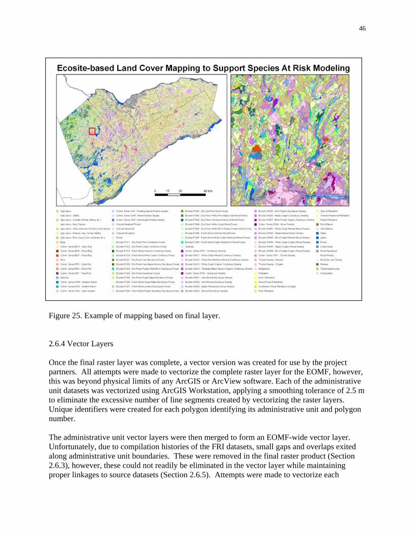
46
Figure 25. Example of mapping based on final layer. 2.6.4 Vector Layers Once the final raster layer was complete, a vector version was created for use by the project partners. All attempts were made to vectorize the complete raster layer for the EOMF, however, this was beyond physical limits of any ArcGIS or ArcView software. Each of the administrative unit datasets was vectorized using ArcGIS Workstation, applying a smoothing tolerance of 2.5 m to eliminate the excessive number of line segments created by vectorizing the raster layers. Unique identifiers were created for each polygon identifying its administrative unit and polygon number. The administrative unit vector layers were then merged to form an EOMF-wide vector layer. Unfortunately, due to compilation histories of the FRI datasets, small gaps and overlaps exited along administrative unit boundaries. These were removed in the final raster product (Section 2.6.3), however, these could not readily be eliminated in the vector layer while maintaining proper linkages to source datasets (Section 2.6.5). Attempts were made to vectorize each

47
administrative unit and a 5 km area beyond each boundary and then “trim” these back using a new common boundary. The smoothing of polygons was slightly different for each area however, creating as many or more slivers than when the datasets were originally combined. A different smoothing algorithm available in ArcMap was explored but created unpredictable slivers throughout the resulting vector datasets. In the end, the raster product provides a seamless layer across the EOMF while the vector product contains small gaps between administrative units but has many other advantages such as linkages to original input data. 2.6.5 Linkages to Original Input Data In the NAESI project, adjacent polygons with the same resulting ecosite class were aggregated in the final layer as a single patch. Modeling that required other attributes from FRI such as age were handled by creating separate grids of the attribute and overlaying to obtain results. For the SAR project we felt a more direct link to the original input data was needed for detailed species modeling and ease of use by the project partners. During the overlay process, a system of coding was devised to maintain the ability to link directly with the original FRI data. The final SAR class was multiplied by 1000. Patches that were derived primarily from FRI, including forest and swamp Ecosites were given an added code created by adding the age, height and stocking of the original FRI polygon. For example, if two adjacent patches were both FOC1 – Dry Fresh Pine Coniferous Forest, their SAR code of 10 was multiplied by 1000 to become 10000. Each patch’s age, height, and stocking values were added together and then added to 10000 to create new unique classes (e.g. 10151 and 10123) to separate the patches while maintaining their identity as an FOC1 patch. The final grid was vectorized based on the new 5-digit codes. The resulting polygons forced the patches to remain separate but by dividing the codes by 1000 and removing remainders, the SAR code was restored. In the final polygon dataset, the adjacent patches maintained their shapes and were not aggregated into a larger patch of FOC1 and could therefore be linked to their original FRI information showing different ages and heights etc. despite the fact that they have the same SAR classification code. The original FRI data was linked to the final SAR polygon dataset by performing an identity overlay of the centroids of the SAR layer polygons with the original FRI layer. With the FRI attribute table joined to the final SAR polygon layer, users now have full access to all of the FRI attributes for polygons that were derived primarily from FRI information (e.g. forest and swamp ecosites). The exact shapes of these polygons vary slightly in the SAR layer due to the filtering and combining with adjacent classes in the overlay process with agriculture, road and other information, however, information about the dominant underlying FRI polygon for each SAR polygon is maintained. A similar identity overlay was used to link the final SAR layer with the new Evaluated Wetland information, allowing users to query and work with the detailed wetland information for SAR polygons derived primarily from the Evaluated Wetland information (e.g. fens, bogs, marshes, aquatics). In the case of swamps, information from both FRI and Evaluated Wetlands often overlap and can be queried together. The boundaries of swamps were defined primarily by FRI information, however, the related wetland polygons for swamps were linked for users to access.

48
This will be important for evaluating cases where discrepancies may exist between the wetland data and the often more spatially detailed FRI data (e.g. wetland data may consider a large area as deciduous swamp while the FRI may show pockets of dominantly conifer swamp). With the linked tables joined to the SAR layer, queries and attribute-based analyses can be performed on SAR classes as well as any of the associated FRI or Evaluated Wetland attributes (Figure 26). A full description of the technical details of joining the linked tables to the SAR layer is provided in the spatial data description (Appendix II). 2.6.6 Linkage to Data Source Names and Dates Examining a detailed section of the final layer (Figure 27) shows the relationship of patches based on FRI, wetlands and other information sources. Attributes were added to the final polygon layer to indicate the source dataset and date of the source polygon or imagery-based data. Some shapes are altered on the landscape due to filtering and filling processes described earlier. All source information is based on the dominant source for each patch and in cases where filling has occurred, the dominant source of the fill is captured. Users should remember this case when comparing the SAR layer with input datasets. For example, if an unknown agricultural area is filled from an adjoining forest class based on FRI, comparing this new shape with the original FRI will not match exactly, however, the dominant source for the filling class is still the FRI-based forest type. 2.7 Updating Layer in the Future One of the primary goals of the mapping project was to create a documented, repeatable process to provide scientific rigour, but also to allow the future custodian of the data a means to update the layer as new information becomes available. The entire process listed above has been captured in a series of GIS scripts and steps to allow data managers in the future to insert new or updated layers, and compile new layers by administrative unit and then across the EOMF as needed. For example, if new Evaluated Wetland information becomes available, this new layer can be inserted in place of the existing layer, combined using the logic and processes in place with the other unchanged layers to create the updated product. While the process is programmed and documented, it remains a very processing intensive task that requires some user inputs and knowledge to complete. We would suggest collecting new information of an annual or semi-annual basis to maintain strict version control of the layer for future distribution. Technical documentation of the process, GIS steps and scripts will be distributed to the final data custodian in a separate technical documentation package.
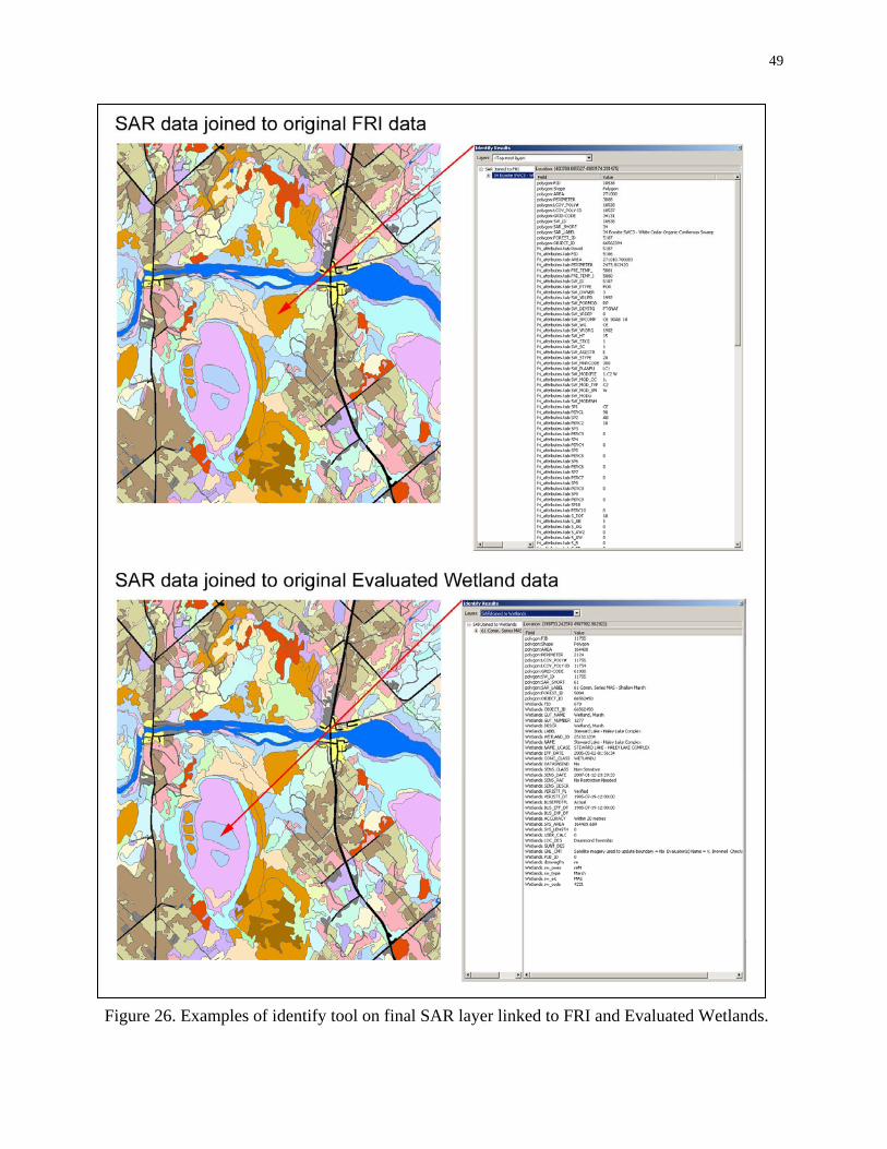
49
Figure 26. Examples of identify tool on final SAR layer linked to FRI and Evaluated Wetlands.
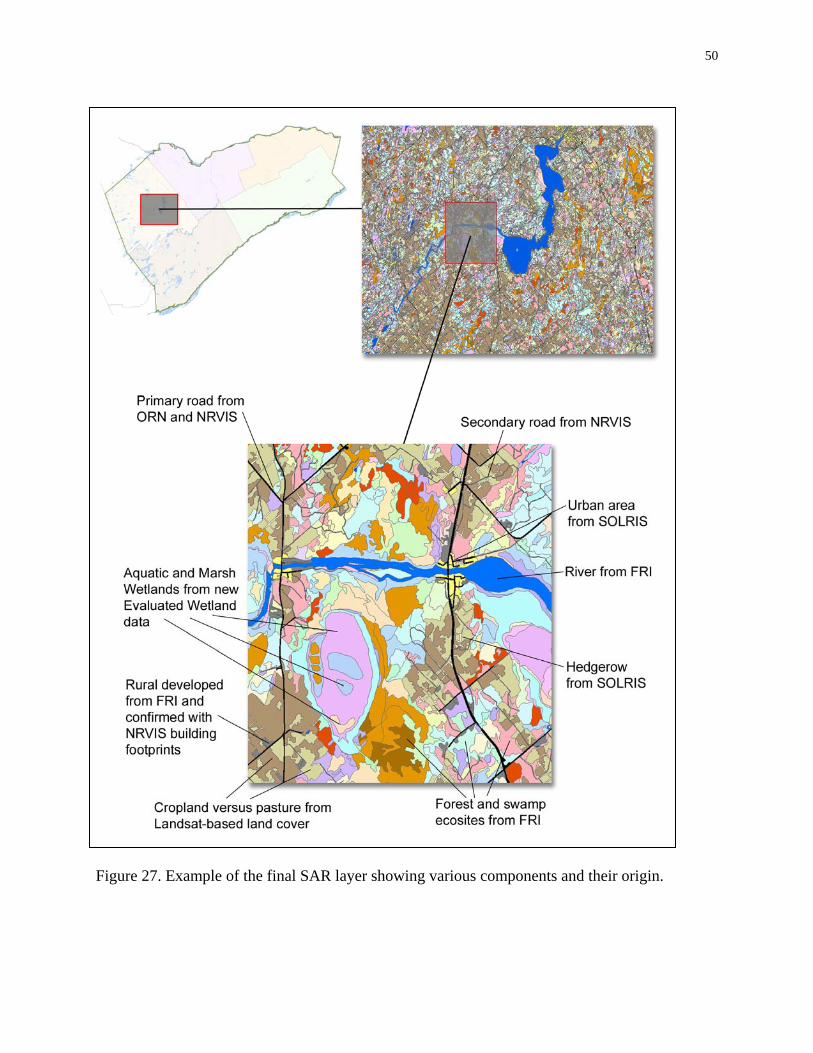
50
Figure 27. Example of the final SAR layer showing various components and their origin.

51
3.0 Habitat Models and Mapping The primary use of the new SAR layer will be for habitat supply mapping / modeling, particularly for Species at Risk. As an example of how the new layer can be used for this purpose, a separate project team (Glenn Desy, Christie Curley, Erin Neave with input from other biologists and steering committee members) developed habitat supply models for four Species at Risk:
- Least Bittern - Red-Headed Woodpecker - Southern Flying Squirrel - Eastern Prairie Fringed-Orchid
Details of these models are included in a separate document (Appendix III). Model descriptions were translated and programmed into spatial habitat models to run against the new SAR layer, including the linked FRI and wetland attributes to create the final habitat maps. Modeling was completed using the seamless raster layer and raster layers created from the polygon layer linked to the FRI data. Processing was completed at 7.5 m resolution to accommodate intermediate floating-point layers less than 2 Gbytes. Once the raster layers of potential, utilized, and preferred habitats were created, raster-based dominance assessment allowed linkage of these values back to the polygon layer for simplified mapping across the EOMF (Appendix III) Examples of these maps (Figures 28-31) show the level of spatial detail that can be achieved using the new layer. While these preliminary models represent relatively simple habitat definitions, more detailed processes and habitat components can be modeled as they are defined for species in the future (e.g. distance functions to water, roads, number and quality of habitat patches within a specified distance of each habitat patch).
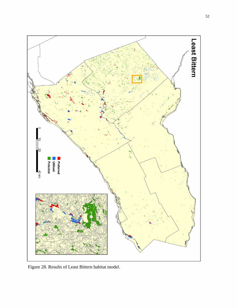
52
Figure 28. Results of Least Bittern habitat model.

53
Figure 29. Results of Red-Headed Woodpecker habitat model.

54
Figure 30. Results of Southern Flying Squirrel habitat model.

55
Figure 31. Results of Eastern Prairie Fringed Orchid habitat model.

56
4.0 Final Deliverables As outlined above, the final deliverables include:
- Spatially referenced Grid format SAR Ecosite-based land cover layer (2m minimum resolution);
- Spatially referenced, Shapefile format polygon version of the SAR Ecosite-based land cover layer including linked tables for FRI, Evaluated Wetlands, and RVCA reforestation site attribute information;
- A documented, repeatable process to allow updating of the SAR land cover layers as new data becomes available;
- GIS-based models for 4 species at risk and output maps and summary values;
4.1 Key Benefits and Potential Uses of the Deliverables The new SAR Ecosite-based land cover layers represent a significant step in bringing together a wide array of natural and anthropogenic land cover data to provide a single integrated context layer for habitat mapping and modeling. Combining forest and wetlands with anthropogenic land uses such as agriculture and roads within the same layer greatly simplifies modeling of spatial constraints among potential habitat and potential barriers or detrimental landscape components for a species. The integrated nature of the new data is also particularly important for modeling movement through the landscape and defining corridors. The information from this project will also support education and outreach and demonstrate the utility of a systems approach to all of the partners of the EOMF by:
- Identifying best potential areas for locating species at risk - Flagging potential habitat for Environmental Impact Assessment in the municipal
planning process - Supporting project-based and landscape-based recovery planning· - Supporting restoration efforts by identifying potential locations of important habitats - Supporting the habitat supply component of population viability analysis (PVA) for
species at risk. All processes used to create the layers are documented and repeatable, facilitating future updating of the complete layer as new input layers become available (e.g. updated FRI, wetland, agricultural classification data). 4.2 Limitations of the SAR Layer As with any data compilation exercise, limitations are closely tied to the input data sources. While the new SAR layers represent a compilation of the best available data for each landscape component, many of these input sources are dated and have limited spatial and thematic resolution, varying across the study area. While we have no control over the quality of the original sources, we have documented the source data used to create each patch and polygon of

57
the new layers so that future updates can be examined against the current state of the data in each location to assess the relative improvement a new data source will offer at that location. Limitations in the spatial accuracy of the source data are represented in spatial misalignments along adjacent land cover or land use types (e.g. where FRI forest meet detailed agricultural classification data). We have employed an innovative approach to combine the various layers and filter out slivers and other anomalies created along boundaries to a significant degree but this can never be completely accurate given the variation in spatial accuracy of the original sources. For this reason the new layers should never be used as an indication of exact land cover composition at a specific location such as a single farm or lot boundary. While many of the input dataset are very spatially accurate, the combination of sources forces the layers to be used as a representation of the best available information to map habitat and other landscape values at a landscape level. 4.3 Planned Combination of SAR Layer with Predicted Vegetation Mapping It was the original intent of the project team to incorporate the recent Predicted Vegetation Mapping (PVM) conducted by the Information Management and Spatial Analysis (IM&SA) Unit, Southern Science and Information Section of OMNR as the most recent forest ecosite information where PVM overlapped with the SAR layer in the south west half of Leeds and Grenville Counties. Upon further analysis, the project team decided that it was more appropriate to keep the two datasets separate given that:
1. PVM covers 39.2 % of the Leeds and Grenville area, resulting in mixed sources and dates of Ecosite information across the administrative unit.
2. The PVM classification provides more detailed classes in many cases that would have to be aggregated to the ecosite level, adding a new component of uncertainty to the forest ecosite information.
3. PVM mapping does not include predictions for transitional types (e.g. Poplar) and coniferous forest that would require a mix of the PVM and FRI-based Ecosite information within the PVM overlap area.
4. Methods and assumptions used to develop the FRI-based and PVM-based forest information are quite different from each other. Combining these sources in the same area would make tracking of sources and their appropriate assumptions and limitations difficult for users if combined within a single layer.
The project team decided it would be more appropriate to keep these layers separate so that their inputs, assumptions, strengths and limitations could be better understood, documented and used for the various mapping and spatial analysis requirements of end users.

58
References Cardille, J.A., and M.K. Clayton. 2007. A regression tree-based method for integrating land-cover and land-use data collected at multiple scales. Environmental and Ecological Statistics. 14: 161-179. Cohen, M.J., Dabral S., Graham W.D., and J.P. Prenger. 2006. Evaluating ecological conditions using soil biogeochemical parameters and near infrared reflectance spectra. Environmental Monitoring and Assessment 116: 427-457. De’ath, G., and K.E. Fabricus. 2000. Classification and regression trees: a powerful yet simple technique for ecological data analysis. Ecology. 81: 3178-3192. Graef, F., Schmidt G., Schroeder W., and U. Stachow. 2005. Determining ecoregions for environmental and GMO monitoring networks. Environmental Monitoring and Assessment. 108: 189-203. Iverson, L.R., and A.M. Prasad. 1998. Predicting abundance of 80 tree species following climate change in the eastern United States. Ecological Monographs. 68: 465-485. Lawler, J.J., and T.C. Edwards. Jr. 2002a. Landscape patterns as predictors of nesting habitat: building and testing models for four species of cavity nesting birds. Landscape Ecology. 17: 233-245. Lee, H.T., W.D. Bakowsky, J. Riley, J. Bowles, M. Puddister, P. Uhlig and S. McMurray. 1998. Ecological Land Classification for Southern Ontario: First Approximation and Its Application. Ontario Ministry of Natural Resources, Southcentral Science Section, Science Development and Transfer Branch. SCSS Field Guide FG-02. Michaelsen, J., Schimel D.S., Friedl M.A., Davis F.W., and R.C. Dubayah. 1994. Regression tree analysis of satellite and terrain data to guide vegetation sampling and surveys. Journal of Vegetation Science. 5: 673-686. Neave E., Baldwin D., Nielsen C. 2008. Tiers 2 and 3 Standards: Habitat-based biodiversity standards decision support process and results of Eastern Ontario Pilot Project - Full Technical Report. National Agri-Environmental Standards Initiative Technical Series. Draft. 633 pages. Perera, A.H., Baker J.A., Band L.E. and D.J.B. Baldwin. 1996. A Strategic Framework to Eco-Regionalize Ontario. Environmental Monitoring and Assessment. 39: 85-96. Robertson, D.M., Saad D.A., and D.M. Heisey. 2005. A Regional Classification Scheme for Estimating Reference Water Quality in Streams Using Land-Use-Adjusted Spatial Regression-Tree Analysis. Environmental Management. 37(2): 209-229.

59
Taverna, K., Urban D.L., and R.I. McDonald. 2004. Modeling landscape vegetation pattern in response to historic land-use: a hypothesis driven approach for the North Carolina Piedmont, USA. Landscape Ecology. 20: 689-702. Wilds., S.P. 1996. Gradient analysis of the distribution of flowering dogwood (Cornus florida L.) and dogwood anthracnose (Discula destructiva Redlin.) in western Great Smoky Mountains National Park. M.S. Thesis, Univ. of North Carolina, Chapel Hill. 151pp.
Wolock, D.M., and G.J McCabe, Jr. 1995. Comparison of single and multiple flow direction algorithms for computing topograhic parameters in TOPMODEL. Water Resources Research 31:1315-1324.

60
Appendix I
Ecosite Assignment Rules


62
NAESI Ecosite Assignment Rules – July 2006VDDT Forest Forest Swamp DF/FM Organic Species Composition Category Class
Num Type Site Dominated Logical Statements FOC1 - Dry-Fresh Pine Coniferous Forest 1001 Yes(1) Conif. (2) No(0) DF (1) No(0) R1: PJ+PW+PR >= 5 or sp1 = 'PW' or sp1 = 'PR' or sp1 = 'PJ'
R2: PW + PJ + PR > 0 and ( PW + PJ + PR ) >= ( CE + SW + B ) FOC2 - Dry-Fresh Cedar Coniferous Forest 1002 Yes(1) Conif. (2) No(0) DF (1) No(0) R1: ( CE + SW + B >= 5 ) or sp1 = 'CE' or sp1 = 'SW' or sp1 = 'B'
R2: ( CE + SW + B ) > ( PW + PJ + PR ) C1: -> 1004 if sw_cl_new = 1002 and ( MS + BD + EW + AB >= 3 )
FOC3 - Fresh-Moist Hemlock Coniferous Forest 1003 Yes(1) Conif. (2) No(0) FM (2) No(0) R1: HE >= 5 and CE <= 2 R2: HE > 0 and HE >= ( CE + B + L + SW + PW )
FOC4 - Fresh-Moist White Cedar Coniferous Forest 1004 Yes(1) Conif. (2) No(0) FM (2) No(0) R1: CE >= 3 or SP1 = 'CE' R2: ( CE + B + SW ) > ( HE + PW ) C1: -> 4004 if sw_cl_new = 1004 and ( sp1 = 'L' or sp1 = 'SB' )
FOM1 - Dry Oak-Pine Mixed Forest 2001 Yes(1) Mixed (3) No(0) DF (1) No(0) R1: ( OW + OR + PW + PR >= 5 ) and ( OW + OR >= 2 ) and ( PW + PR < 8 ) R2: (OW + OR + PW + PR + PS >= 5) and ( ( OW + OR ) > ( PW + PR + PS ) )
FOM2 - Dry-Fresh White Pine-Maple-Oak Mixed Forest 2002 Yes(1) Mixed (3) No(0) DF (1) No(0) R1: PW + MH + OR >= 5 and PW > MH and PW > OR R2: sp1 = 'PW' or ( PW > MH and PW > HE and pw > CE ) or PW >= 3
FOM3 - Dry-Fresh Hardwood-Hemlock Mixed Forest 2003 Yes(1) Mixed (3) No(0) DF (1) No(0) R1: HE + MH + OR >= 5 and HE >= 4 R2: sp1 = 'HE' or sp1 = 'MH' or ( ( HE > PW and HE > CE ) or ( MH > PW and MH > CE ) )
FOM4 - Dry-Fresh White Cedar Mixed Forest 2004 Yes(1) Mixed (3) No(0) DF (1) No(0) R1: CE + BW + PO + PL + MH + AW >= 5 and CE >= 3 R2: sp1 = 'CE' or ( CE > PW and CE > HE and CE > MH ) C1: -> 2007 if sw_cl_new = 2004 and ( MS + BD + EW + AB + BY >= 3 ) C2: -> 2005 if sw_cl_new = 2004 and ( po > ce )
FOM5 - Dry-Fresh White Birch-Poplar-Conifer Mixed Forest
2005 Yes(1) Mixed (3) No(0) DF (1) No(0) R1: BW + PO + PL + B + PW + SW >= 5 and BW + PO + PL >= 3 R2: sp1 = 'BW' or sp1 = 'PO' or sp1 = 'PL' or sp1 = 'B' C1: -> 2004 if sw_cl_new = 2005 and CE >= 3
FOM6 - Fresh-Moist Hemlock Mixed Forest 2006 Yes(1) Mixed (3) No(0) FM (2) No(0) R1: HE + MH + BY >= 5 and ( HE + MH > BY ) and he >= 3 R2: sp1 = 'HE' or sp1 = 'MH' or sp1 = 'MS' C1: -> 4004 if sw_cl_new = 2006 and sp1 = 'MS' and HE <= 2
FOM7 - Fresh-Moist White Cedar-Hardwood Mixed Forest 2007 Yes(1) Mixed (3) No(0) FM (2) No(0) R1: CE + BY + MS >= 5 and CE >= 3 and MS + AB <= 2 R2: sp1 = 'CE' or sp1 = 'BY' or sp1 = 'B'
FOM8 - Fresh-Moist Poplar-White Birch Mixed Forest 2008 Yes(1) Mixed (3) No(0) FM (2) No(0) R1: PO + PL + BW >= 5 and B + HE + SB >= 3 R2: sp1 = 'PO' or sp1 = 'PL' or sp1 = 'BW' or sp1 = 'B' C1: -> 2007 if sw_cl_new = 2008 and CE >= 3
FOD2 - Dry-Fresh Oak-Maple-Hickory Deciduous Forest 3002 Yes(1) Decid. (1) No(0) DF (1) No(0) R1: ( sp1 = 'OW' or sp1 = 'OR' ) and ( HI + AW + BE + BD + IW > 1 ) and MH <= 3 and OW + OR >= 4 C1: -> 3005 if sw_cl_new = 3002 and ( OR + OW < 1 )
FOD1 - Dry-Fresh Oak Deciduous Forest 3001 Yes(1) Decid. (1) No(0) DF (1) No(0) R1: sp1 = 'OW' or sp1 = 'OR' or OR + OW >= 4 R2: sp1 = 'OW' or sp1 = 'OR'
Forest
FOD3 - Dry-Fresh Poplar-White Birch Deciduous Forest 3003 Yes(1) Decid. (1) No(0) DF (1) No(0) R1: sp1 = 'PO' or sp1 = 'PL' or sp1 = 'BW' and PO + PL + BW >= 4 R2: sp1 = 'PO' or sp1 = 'PL' or sp1 = 'BW' or sp1 = 'EW' or sp1 = 'BG' C1: -> 3007 if sw_cl_new = 3003 and ( MS + BD + EW + AB + BY >= 3 )

63
FOD4 - Dry-Fresh Deciduous Forest 3004 Yes(1) Decid. (1) No(0) DF (1) No(0) R1: sp1 = 'AW' or sp1 = 'BE' C1: -> 3005 if sw_cl_new = 3004 and MH >= 2
FOD5 - Dry-Fresh Sugar Maple Deciduous Forest 3005 Yes(1) Decid. (1) No(0) DF (1) No(0) R1: MH + BE + OR + OW + IW + BD + CB + HI + PO + PL + AW >= 5 and ( sp1 = 'MH' or sp2 = 'MH' ) R2: sp1 = 'MH' or sp1 = 'IW' or sp1 = 'BD' or sp1 = ‘HI’
FOD7 - Fresh-Moist Lowland Deciduous Forest 3007 Yes(1) Decid. (1) No(0) FM (2) No(0) R1: EW + W + WB + WI + AB + AG + BD >= 5 and MH < 3 R2: sp1 = 'EW' or sp1 = 'AG' or sp1 = 'AB' or sp1 = 'BD' C1: -> 3008 if sw_cl_new = 3007 and sp1 = ‘PO’ C2: -> 4012 if sw_cl_new = 3007 and AB + AG >= 5 C3: -> 4005 if sw_cl_new = 3007 and sp1 = ‘CE’ C4: -> 4013 if sw_cl_new = 3007 and sp1 = ‘MS’
FOD6 - Fresh-Moist Sugar Maple Deciduous Forest 3006 Yes(1) Decid. (1) No(0) FM (2) No(0) R1: MH + MS + AB + EW + BY + BD + BE >= 5 and ( MH >= 3 or SP1 = 'MH' or SP2 = 'MH' ) and MS + AB <= 2 R2: sp1 = 'BY' or sp1 = 'BE' or sp1 = 'MH' C1: -> 3004 if sw_cl_new = 3006 and (AW >= 4 ) and ( MS + BD + EW + AB + BY < 2 ) C2: -> 4013 if sw_cl_new = 3006 and MH < 2
FOD8 - Fresh-Moist Poplar-Sassafras Deciduous Forest 3008 Yes(1) Decid. (1) No(0) FM (2) No(0) R1: sp1 = ( 'PO' or sp1 = 'PL' ) and PO + PL >= 4 R2: sp1 = 'PO' or sp1 = 'PL' or sp1 = 'BW' or sp1 = 'BG'
SWC1 - White Cedar Mineral Coniferous Swamp 4001 - Conif. (2) Yes(1) -
No(0) R1: CE > 0 and ( ( CE + L + SW + B >= 5 ) or ( sp1 = 'CE' or sp1 = 'B' or sp1 = 'SW' ) ) R2: ( CE + B + SW ) > 0 and ( ( CE + SW + B ) >= ( PW + HE ) or ( CE + SW + B ) >= ( L ) )
SWC2 - White Pine-Hemlock Mineral Coniferous Swamp 4002 - Conif. (2) Yes(1) - No(0) R1: ( PW + HE >= 5 ) or sp1 = 'PW' or sp1 = 'HE' R2: ( PW + HE ) > ( CE + B + SW )
SWC4 - Tamarack-Black Spruce Organic Conifer. Swamp 4004 - Conif. (2) Yes(1) - Yes(1) R1: ( L + SB >= 5 ) or sp1 = 'SB' or sp1 = 'L' R2: ( L + SB > 0 ) and ( L + SB ) >= ( CE + SW + B + PW )
SWC3 - White Cedar Organic Coniferous Swamp 4003 - Conif. (2) Yes(1) - Yes(1) R1: CE > 0 and ( ( CE + L + SW + B >= 5 ) or ( sp1 = 'CE' or sp1 = 'B' or sp1 = 'SW' ) ) R2: ( CE + B + SW ) > 0 and ( ( CE + SW + B ) >= ( PW + HE ) or ( CE + SW + B ) >= ( L ) )
SWM1 - White Cedar Mineral Mixed Swamp 4005 - Mixed (3) Yes(1) - No(0) R1: ( ( CE + AB + AG + EW + BY + MS >= 3 ) and CE >= 3 and MS < 4 ) or sp1 = 'CE' R2: sp1 = 'CE' or sp1 = 'AB' or sp1 = ‘B’ or sp1 = ‘AG’ or ( CE > MS and CE > BW and CE > BY and CE > PO )
SWM2 - Maple Mineral Mixed Swamp 4006 - Mixed (3) Yes(1) - No(0) R1: ( MS >= 5 ) or sp1 = 'MS' R2: sp1 = 'MS' or ( MS > CE and MS > BW and MS > BY and MS > PO ) C1: -> 4005 if sw_cl_new = 4006 and CE >= 3
SWM3 - Birch-Poplar Mineral Mixed Swamp 4007 - Mixed (3) Yes(1) - No(0) R1: ( BW + BY + PO >= 5 ) or sp1 = 'BW' or sp1 = 'BY' or sp1 = 'PO' R2: sp1 = 'BY' or sp1 = 'PO' or ( ( BY + BW + PO + PB + PW ) > ( MS + CE) )
Swamp
SWM4 - White Cedar Organic Mixed Swamp 4008 - Mixed (3) Yes(1) - Yes(1) R1: ( ( CE + AB + AG + EW + BY + MS >= 3 ) and CE >= 3 and MS < 4 ) or sp1 = 'CE' R2: sp1 = 'CE' or sp1 = 'AB' or sp1 = ‘B’ or sp1 = ‘AG’ or ( CE > MS and CE > BW and CE > BY and CE > PO )

64
SWM5 - Maple Organic Mixed Swamp 4009 - Mixed (3) Yes(1) - Yes(1) R1: ( MS >= 5 ) or sp1 = 'MS' R2: sp1 = 'MS' or ( MS > CE and MS > BW and MS > BY and MS > PO ) C1: -> 4008 if sw_cl_new = 4009 and CE > 2
SWM6 - Birch-Poplar Organic Mixed Swamp 4010 - Mixed (3) Yes(1) - Yes(1) R1: ( BW + BY + PO >= 5 ) or sp1 = 'BW' or sp1 = 'BY' or sp1 = 'PO' R2: sp1 = 'BY' or sp1 = 'PO' or ( ( BY + BW + PO + PB + PW ) > ( MS + CE) )
SWD1 - Oak Mineral Deciduous Swamp 4011 - Decid. (1) Yes(1) - No(0) R1: OW + MS + EW + HI >= 5 and sp1 = 'OW'
SWD3 - Maple Mineral Deciduous Swamp 4013 - Decid. (1) Yes(1) - No(0) R1: sp1 = 'MS' C1: -> 4014 if sw_cl_new = 4013 and sp1 = ‘PO’ or sp1 = ‘BY’
SWD2 - Ash Mineral Deciduous Swamp 4012 - Decid. (1) Yes(1) - No(0) R1: AB + AG + EW + MS >= 5 or sp1 = 'AB' or sp1 = 'AG' R2: sp1 = 'AW' and MS + BD + AB >= 3 C1: -> 4014 if sw_cl_new = 4012 and sp1 = ‘BY’ or sp1 = ‘BW’ or sp1 = ‘BG’ or sp1 = ‘PO’ or sp1 = ‘EW’ C2: -> 4005 if sw_cl_new = 4012 and CE >= 3 or sp1 = ‘CE’ C3: -> 3006 if sw_cl_new = 4012 and sp1 = ‘MH’
SWD4 - Mineral Deciduous Swamp 4014 - Decid. (1) Yes(1) - No(0) R1: W + WI + EW + BW + BY + PO + PB >= 5 R2: sp1 = 'BW' or sp1 = 'BY' or sp1 = 'PO' or sp1 = 'PB' or sp1 = 'BG' R3: sp1 = 'EW' and MH <= 2 C1: -> 3004 if sw_cl_new = 4014 and sp1 = ‘AG’ and MH > 0 C2: -> 3005 if sw_cl_new = 4014 and sp1 = ‘AW’ and MH = 0 C3: -> 3006 if sw_cl_new = 4014 and sp1 = ‘MH’
SWD6 - Maple Organic Deciduous Swamp 4016 - Decid. (1) Yes(1) - Yes(1) R1: sp1 = 'MS' C1: -> 4015 if sw_cl_new = 4016 and sp1 = ‘AW’ or sp1 = ‘AB’ C2: -> 4017 if sw_cl_new = 4016 and sp1 = ‘BW’
SWD5 - Ash Organic Deciduous Swamp 4015 - Decid. (1) Yes(1) - Yes(1) R1: AB + AG + EW + MS >= 5 or sp1 = 'AB' or sp1 = 'AG' C1: -> 4017 if sw_cl_new = 4015 and sp1 = ‘PO’ or sp1 = ‘BW’
SWD7 - Birch-Poplar Organic Deciduous Swamp 4017 - Decid. (1) Yes(1) - Yes(1) R1: W + WI + EW + BW + BY + PO + PB >= 5 R2: sp1 = 'BW' or sp1 = 'BY' or sp1 = 'PO' or sp1 = 'PB' or sp1 = 'BG'
Notes - Stands are assigned to their broad groups(colours) before species queries are executed
- R1 queries are executed in order shown within broad group
- Once stands are assigned an ecosite they are not available for further selection
- R2,3,.. N queries are executed after all group R1 queries are complete
- C1,2,.. N adjust initial results to other classes after R1 and R2,3 queries are complete
- Minor manual assignments are made for stands that remain unclassified within a broad group

65
65
Appendix II
Spatial Database Description

66
66
1.0 Introduction The following describes the structure of spatial data products for the Species at Risk (SAR) mapping project for the Eastern Ontario Model Forest (EOMF) including:
- Seamless raster (ESRI GRID format) of ecosite-level classes across the EOMF and divided by administrative units and Conservation Authority boundaries
- Polygon datasets (ESRI Shapefile format) for the entire EOMF and divided by administrative units and Conservation Authority boundaries containing fields for:
o Ecosite-level numeric classes and character class names o Dominant data source name (e.g. FRI, Evaluated Wetlands, NRVIS)
and source date for each polygon o Area in hectares o Key fields to link to:
Original FRI attributes Standardized FRI across the EOMF Evaluated Wetlands Rideau Valley Conservation Authority reforestation sites SAR model outputs
- Species at Risk model outputs in both raster (ESRI GRID format) and linked tables (Dbase format) for polygon datasets
- Tabular data (Dbase format) for all linked data (FRI, Wetlands, RVCA reforestation sites, SAR model outputs)
Complete documentation for how these spatial products were derived is available in the main project report.
67
67
2.0 Data Structure The data distribution set contains three main directories: /SAR_Grids /SAR_Shapefiles /SAR_Linked_Data 2.1 SAR Grids The /SAR_Grids directory contains all of the raster-based of the final ecosite-level classification as well as the model outputs from the four sample SAR habitat models. 2.1.1 Ecosite-level Classification Grids Rasters were created based on the SAR project Ecosite-level classification (Appendix I). Note that the classes are hierarchical, to reflect the best available data in each location. For example, in some cases swamps may be classified to the Ecosite-level while in others, data may only have been available to classify to the Community Series or to the Swamp class. Users should determine which level of classification they wish to aggregate the data depending on the level available in their study area. All rasters are in ESRI GRID format at 2m resolution. Each raster has been coded with numeric classes corresponding to the final SAR ecosite-based classification. Ecosite-level Classification Grids are contained within the /SAR_Grids directory in three ArcGIS workspaces: /SAR_Grids/Administrative_Units /SAR_Grids/Conservation_Authorities /SAR_Grids/EOMF_Wide Each workspace consists of the directories for each grid (containing grid internal files) and an info directory (containing internal tabular and referencing information). This structure must be maintained for GRIDS to be accessible. GRIDS should only be moved as a unit (e.g. entire workspace structure) or copied within ArcGIS. For example, copying only the lanark_sar directory to a new location will not allow users to access the GRID data. GRIDS have been created for a variety of extents to allow users to work with their study area or the entire EOMF as required. GRIDS available in this distribution include: /SAR_Grids/EOMF_Wide/eomf_sar - 2m grid for the entire EOMF /SAR_Grids/Administrative_Units/lanark_sar

68
68
- 2m grid for Lanark County /SAR_Grids/Administrative_Units/leeds_sar - 2m grid for Leeds and Grenville Counties /SAR_Grids/Administrative_Units/ottawa_sar - 2m grid for City of Ottawa /SAR_Grids/Administrative_Units/prescott_sar - 2m grid for Prescott and Russell Counties /SAR_Grids/Administrative_Units/sdg_sar - 2m grid for Stormont, Dundas, and Glengarry Counties /SAR_Grids/Conservation Authorities/crca_sar - 2m grid for Cataraqui Region Conservation Authority, including a 5km buffer of data /SAR_Grids/Conservation Authorities/mvca_sar - 2m grid for Mississippi Valley Conservation Authority, including a 5km buffer of data /SAR_Grids/Conservation Authorities/rrca_sar - 2m grid for Raisin Region Conservation Authority, including a 5km buffer of data /SAR_Grids/Conservation Authorities/rvca_sar - 2m grid for Rideau Valley Conservation Authority, including a 5km buffer of data /SAR_Grids/Conservation Authorities/snca_sar - 2m grid for South Nation Conservation Authority, including a 5km buffer of data Please note that many of the extents represent significantly large areas and corresponding file sizes at 2m resolution. In many cases, using these grids in modeling where floating-point values are required (e.g. calculating a grid of distance from water bodies) will result in grids greater than 2Gbytes in size. This is beyond a physical limit for ArcGIS versions 8.X and users will have to subset the original grid prior to analysis or use ArcGIS version 9.X 2.1.2 SAR Habitat Model Output GRIDS Rasters have been included for the results of the four example SAR habitat models across the EOMF. Modeling was carried out using a resolution of 7.5 m to allow floating point grids < 2Gbytes while providing sufficient spatial detail for model outputs. Details of the habitat model development and implementation are contained in the complete project report. GRIDS contain binary values for Potential, Utilized, and Preferred for Eastern Fringed Prairie Orchid, Least Bittern and Southern Flying Squirrel and binary values for

69
69
Utilized and Preferred for Red-Headed Woodpecker. Model results were also associated with the final polygon dataset using a raster-based dominance method to create tables of model results to link with each polygon (Section 2.2). The GRIDS available in this distribution include: /SAR_Grids/SAR_Habitat_Models/eomf_bit_po - 7.5 m grid of Potential Habitat (value=1) for Least Bittern across the EOMF /SAR_Grids/SAR_Habitat_Models/eomf_bit_ut - 7.5 m grid of Utilized Habitat (value=1) for Least Bittern across the EOMF /SAR_Grids/SAR_Habitat_Models/eomf_bit_pr - 7.5 m grid of Preferred Habitat (value=1) for Least Bittern across the EOMF /SAR_Grids/SAR_Habitat_Models/eomf_orch_po - 7.5 m grid of Potential Habitat (value=1) for Eastern Fringed Prairie Orchid across the EOMF /SAR_Grids/SAR_Habitat_Models/eomf_orch_ut - 7.5 m grid of Utilized Habitat (value=1) for Eastern Fringed Prairie Orchid across the EOMF /SAR_Grids/SAR_Habitat_Models/eomf_orch_pr - 7.5 m grid of Preferred Habitat (value=1) for Eastern Fringed Prairie Orchid across the EOMF /SAR_Grids/SAR_Habitat_Models/eomf_squir_po - 7.5 m grid of Potential Habitat (value=1) for Southern Flying Squirrel across the EOMF /SAR_Grids/SAR_Habitat_Models/eomf_squir_ut - 7.5 m grid of Utilized Habitat (value=1) for Southern Flying Squirrel across the EOMF /SAR_Grids/SAR_Habitat_Models/eomf_squir_pr - 7.5 m grid of Preferred Habitat (value=1) for Southern Flying Squirrel across the EOMF /SAR_Grids/SAR_Habitat_Models/eomf_wpk_ut - 7.5 m grid of Utilized Habitat (value=1) for Red-Headed Woodpecker across the EOMF /SAR_Grids/SAR_Habitat_Models/eomf_wpk_pr - 7.5 m grid of Preferred Habitat (value=1) for Red-Headed Woodpecker across the EOMF 2.2 SAR Shapefiles

70
70
The /SAR_Shapefiles directory contains all of the polygon-based data for the SAR Ecosite-based classification. These shapefiles were created following the raster-based processing of the various source datasets (described in detail in the full project report). The compilation process maintained direct links to many of the source datasets and consequently key fields were added to the shapefiles to link to many of the original source datasets including FRI, Evaluated Wetlands, RVCA reforestation sites and SAR habitat model results. All shapefiles contain the following field structure: FID Internal ESRI field SHAPE Internal ESRI field GRID_CODE Original coding from the compilation process to assign ecosite
classes and maintain linkages SAR_ID Unique identifier within administrative unit SAR_UNIT Administrative Unit name OBJECT_ID Key field to link with Evaluated Wetlands data (Section 2.3) SAR_RFID Key field to link with RVCA Reforestation data (Section 2.3) SAR_NUM SAR Ecosite-based Classification numeric code (See Appendix I) SAR_NAME SAR Ecosite-based Classification name (See Appendix I) SAR_FRISTD Key field to link with Standardized FRI data (Section 2.3) SAR_FRI_ID Key field to link with original Administrative Unit FRI data (Section 2.3) SRC_NUM Dominant source dataset numeric code (Section 2.3) SRC_DATE Dominant source dataset year (Section 2.3) SRC_NAME Dominant source dataset name (Section 2.3) AREA_HA Area in hectares MODEL_ID Key field to link with SAR habitat model outputs (Section 2.3).
This field is included only in the EOMF-wide shapefile Shapefiles were created for the same extents as the GRIDS to allow use by study area. Again, users should be aware of the large size of many of these datasets when attempting detailed spatial modeling and analyses. Shapefiles available in this distribution include: /SAR_Shapefiles/EOMF_Wide/eomf_sar - Polygon shapefile for the entire EOMF /SAR_Shapefiles/Administrative_Units/lanark_sar - Polygon shapefile for Lanark County /SAR_Shapefiles/Administrative_Units/leeds_sar - Polygon shapefile for Leeds and Grenville Counties /SAR_Shapefiles/Administrative_Units/ottawa_sar - Polygon shapefile for City of Ottawa /SAR_Shapefiles/Administrative_Units/prescott_sar

71
71
- Polygon shapefile for Prescott and Russell Counties /SAR_Shapefiles/Administrative_Units/sdg_sar - Polygon shapefile for Stormont, Dundas, and Glengarry Counties /SAR_Shapefiles/Conservation Authorities/crca_sar - Polygon shapefile for Cataraqui Region Conservation Authority, including a 5km buffer of data /SAR_Shapefiles/Conservation Authorities/mvca_sar - Polygon shapefile for Mississippi Valley Conservation Authority, including a 5km buffer of data /SAR_Shapefiles/Conservation Authorities/rrca_sar - Polygon shapefile for Raisin Region Conservation Authority, including a 5km buffer of data /SAR_Shapefiles/Conservation Authorities/rvca_sar - Polygon shapefile for Rideau Valley Conservation Authority, including a 5km buffer of data /SAR_Shapefiles/Conservation Authorities/snca_sar - Polygon shapefile for South Nation Conservation Authority, including a 5km buffer of data 2.3 SAR Linked Tabular Data The compilation process employed in this project (detailed in the complete project report) allowed direct linkages with many of the input source datasets. For example in forested areas, FRI was usually the definitive source dataset and the patch shapes were essentially maintained through a coding system in the raster-based process. In cases where datasets overlapped, filtering often changed some of the original boundaries, however the coding system and various logical and spatial queries were used to determine the dominant source for the resulting patches. The dominant source and its date were included directly in the polygon shapefiles (Section 2.2) to allow users to determine the confidence level of the information based on the source’s known/perceived accuracy and its date (e.g. FRI varies from 1980 to 1991 across the study area). Complete references and source descriptions are found in the full project report. The following numeric codes and source names and dates are included in the polygons:
Code Source Name Year1 Enhanced FRI Lanark 19912 Enhanced FRI SDG 19913 FRI Prescott Russell 19804 FRI Ottawa 1980

72
72
5 FRI Leeds Grenville 19806 SOLRIS Interim Woodlands 20027 SOLRIS Interim Urban 20028 SOLRIS Version 1-2 20029 AAFC Detailed Crop Classification 2001
10 Ontario Land Cover (Landsat) 199211 Ottawa Land Use 200512 Evaluated Wetlands Various13 Ontario Road Network 200714 RVCA Reforestation Data 200815 NRVIS Base Data 199016 SAR Rural Developed Rule 200817 SAR SOLRIS Rule 200818 Unknown 9998
Actual attribute data for many of these sources can be accessed for each polygon by joining one or more of the included series of tables (Dbase format) within ArcGIS. Once tables are linked users can access the external attributes to perform more detailed and powerful queries than those based on the SAR Ecosite-based classification alone. For example, users could query to find a specific forest Ecosite and then refine the search based on a specific species component from the FRI attribute table. The following tables have been included in this distribution: \SAR_Linked_Data\Evaluated_Wetlands\Evaluated_Wetlands.dbf - OMNR Evaluated Wetlands data, linked to shapefiles based on OBJECT_ID field \SAR_Linked_Data\FRI_Original\FRI_Lanark.dbf - Original FRI data for Lanark County, linked to shapefiles based on SAR_FRI_ID field \SAR_Linked_Data\FRI_Original\FRI_Leeds.dbf - Original FRI data for Leeds and Grenville Counties, linked to shapefiles based on SAR_FRI_ID field \SAR_Linked_Data\FRI_Original\FRI_Ottawa.dbf - Original FRI data for City of Ottawa, linked to shapefiles based on SAR_FRI_ID field \SAR_Linked_Data\FRI_Original\FRI_Prescott.dbf - Original FRI data for Prescott and Russell Counties, linked to shapefiles based on SAR_FRI_ID field \SAR_Linked_Data\FRI_Original\FRI_SDG.dbf - Original FRI data for Stormont, Dundas, and Glengarry Counties, linked to shapefiles based on SAR_FRI_ID field \SAR_Linked_Data\FRI_Standardized\FRI_Standardized_EOMF.dbf

73
73
- A standardized set of FRI attributes across the EOMF, linked to shapefiles based on SAR_FRISTD field \SAR_Linked_Data\RVCA_Reforestation\RVCA_Reforestation.dbf - RVCA_Reforestation Site identifiers, linked to shapefiles based on SAR_RFID field Results of the SAR species habitat models have also been included as tables that can be linked to the EOMF-wide polygon shapefile. SAR habitat result tables included in this distribution include: \SAR_Linked_Data\SAR_Habitat_Models\Eastern_Fringed_Prairie_Orchid.dbf - SAR species habitat model for Eastern Fringed Prairie Orchid, linked to EOMF_SAR shapefile based on MODEL_ID field \SAR_Linked_Data\SAR_Habitat_Models\Least_Bittern.dbf - SAR species habitat model for Least Bittern, linked to EOMF_SAR shapefile based on MODEL_ID field \SAR_Linked_Data\SAR_Habitat_Models\Sothern_Flying_Squirrel.dbf - SAR species habitat model for Southern Flying Squirrel, linked to EOMF_SAR shapefile based on MODEL_ID field \SAR_Linked_Data\SAR_Habitat_Models\Red-Headed_Woodpecker.dbf - SAR species habitat model for Red-Headed Woodpecker, linked to EOMF_SAR shapefile based on MODEL_ID field

74
74
3.0 Questions, Contact Information Users are urged to read the complete project report to obtain details on the compilation and history of the data in this distribution as well as the strengths and limitation of the various datasets. For further information contact: Allen Bibby Geomatics Coordinator OMNR Kemptville District 10 Campus Drive Kemptville, ON (613) 258-8372 Fax: (613)258-3920 [email protected] or David Baldwin Spatialworks 1232 Old Garden River Road Sault Ste. Marie, ON (705) 253-4487

75
75
Appendix III
Protocol for Developing Species at Risk Habitat Suitability Models

76
76
2007 / 08 Protocol for Developing Species at Risk Habitat Suitability Models
for the 2007 / 08 SAR Stewardship Fund Project titled: Predicting Habitat for Eastern Ontario Species at Risk
Protocols and this summary document created by: Glenn Desy, Natural Heritage Biologist Intern, and Christie Curley, Area Biologist for Kemptville District MNR Outline:
1. Goals
2. Species selection
3. Development of wetland data (OWES conversion to ELC)
4. Species-specific parameter selection and model development
5. Sources cited
6. Appendices
Shaun Thompson’s species selection documentation
Final models for the four species
Draft working-table for selecting species-specific parameters
Sample HSM maps for Least Bittern

77
77
GOALS
Overall project goals, excerpt from the 2007 / 08 SAR Stewardship Application:
To develop a coordinated, landscape approach for species at risk habitat mapping for the identification of stewardship opportunities for species at risk in eastern Ontario through the application of the best available science and information. and To promote a Natural Heritage Systems approach to species at risk conservation that:
takes into account the entire landscape when identifying priorities, informs decision making on matters that affect species at risk, and identifies opportunities to ensure effective use of limited resources for stewardship
and recovery.
SAR habitat mapping goals, paraphrased from the 2007 / 08 SAR Stewardship Application:
To develop potential habitat maps for four proposed SAR to demonstrate and test the proposed approach: Butternut, Southern Flying Squirrel, Short-eared Owl, and Red-headed Woodpecker. The species selected may change, but these are suggested because:
They can be mapped using current information. They have a range in habitat requirements (grasslands and forests, area
sensitivities). There is existing habitat relationship information for developing habitat models for
demonstration.

78
78
SPECIES SELECTION
The four species selected for habitat suitability modelling (HSM) in 2007 / 08 were:
1. Least Bittern – Threatened, wetland dwelling bird
2. Southern Flying Squirrel – Special Concern, forest dwelling mammal
3. Eastern Prairie White-fringed Orchid – Endangered, wetland occurring plant
4. Red-headed Woodpecker – Special Concern, forest dwelling bird
Species were selected in accordance with input received from a Species Selection Steering Committee that included representatives from the Kemptville MNR, Rideau Valley Conservation Authority, Parks Canada, and a SAR habitat modelling consultant. A list of relevant criteria were developed against which potential species were evaluated, with the goal of choosing species that would provide a strong demonstration of the functionality of the newly developed “seamless Ecological Land Classification (ELC) digital data layer.” The selection criteria included:
Official Ontario species designation Extent of geographic distribution in district Availability of necessary data Are existing HSM’s available? Is the species a habitat specialist? Is the species influenced by habitat stressors? Does the species display area sensitivity? Are there landscape-level influences to the species’ distribution? Are there stand-level influences to the species’ distribution?
Ideal demonstration species would represent a range of species designations, occur across varied geographic areas of the District, have appropriate data relatively available for modelling, have accessible existing habitat models for reference, be habitat specialists, be influence by habitat stressors, be area sensitive, and have both landscape and stand-level habitat influences. Refer to the following pages for a presentation of the selection criteria as applied to Kemptville District SAR in 2007 / 08. Note that particular consideration was also given to a document developed by Shaun Thompson for use in selecting species for a concurrent SAR habitat modelling project for an area around St. Lawrence Islands National Park (see Appendix 1).
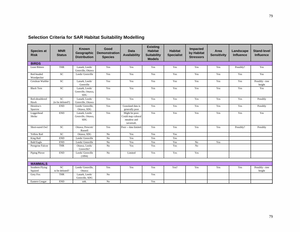
79
79
Selection Criteria for SAR Habitat Suitability Modelling
Species at Risk
MNRStatus
Known Geographic Distribution
Good Demonstration
Species
Data Availability
Existing Habitat
Suitability Models
Habitat Specialist
Impacted by Habitat Stressors
Area Sensitivity
Landscape Influence
Stand-level Influence
BIRDSLeast Bittern THR Lanark, Leeds/
Grenville, OttawaYes Yes Yes Yes Yes Yes Possibly? Yes
Red-headed Woodpecker
SC Leeds/ Grenville Yes Yes Yes Yes Yes Yes Yes Yes
Cerulean Warbler SC Lanark, Leeds/ Grenville
Yes Yes Yes Yes Yes Yes Yes Possibly - tree height
Black Tern SC Lanark, Leeds/ Grenville, Ottawa,
SDG
Yes Yes Yes Yes Yes Yes Yes Yes
Red-shouldered Hawk
SC(to be delisted?)
Lanark, Leeds/ Grenville, Ottawa
Yes Yes Yes Yes Yes Yes Yes Possibly
Henslow's Sparrow
END Leeds/ Grenville, Ottawa, SDG
Yes Grassland data is generally poor
Yes Yes Yes Yes Yes Possibly
Loggerhead Shrike
END Lanark, Leeds/ Grenville, Ottawa,
SDG
Yes Might be poor. Could map cultural
meadow and savannah.
Yes Yes Yes Yes Yes Yes
Short-eared Owl SC Ottawa, Prescott/ Russell
Yes Poor -- data limited. Yes Yes Yes Yes Possibly? Possibly
Yellow Rail SC Ottawa, SDG No Yes Yes Yes
King Rail END Leeds/ Grenville No Yes Yes Yes
Bald Eagle END Leeds/ Grenville No Yes Yes Yes No YesPeregrine Falcon THR Ottawa, Leeds/
Grenville?No Yes Yes Yes No
Piping Plover END Leeds/ Grenville (1894)
No Limited Yes Yes Yes
MAMMALSSouthern Flying Squirrel
SCto be delisted?
Leeds/ Grenville, Ottawa
Yes Yes Yes Yes? Yes Yes Yes Possibly - tree height
Grey Fox THR Lanark, Leeds/ Grenville, SDG
No Yes
Eastern Cougar END unk. No Yes

80
80
Species at Risk
MNR StatusKnown
Geographic Distribution
Good Demonstration
Species
Data Availability
Existing Habitat
Suitability Models
Habitat Specialist
Impacted by Habitat
Stressors
Area Sensitivity
Landscape Influence
Stand-level Influence
REPTILESFive-lined Skink SC Lanark, Leeds/
GrenvilleYes Somewhat Yes Yes? Yes No? No? microhabitat
requirements are impossible to model
Blanding's Turtle THR Lanark, Leeds/ Grenville, Ottawa
No No Yes
Spiny Softshell THR Leeds/ Grenville, Prescott/ Russell
No No Yes
Eastern Ratsnake SC Lanark, Leeds/ Grenville
No No Yes No Yes May be limited by available nesting
sites
Spotted Turtle END Leeds/ Grenville, Ottawa, Prescott/
Russell
No No Yes
Stinkpot THR Lanark, Leeds/ Grenville, Ottawa
No No Might be similar to painted turtle,
which did not work well for Erin Neave.
Wood Turtle END Lanark, Ottawa, Leeds/ Grenville
No No Yes No
Eastern Ribbon Snake
SC Lanark, Leeds/ Grenville, Ottawa
No No Yes
Milksnake SC Lanark, Leeds/ Grenville, Ottawa
No No Yes No
Northern Map Turtle
SC Lanark, Leeds/ Grenville, Ottawa
No No No? Unclear Apparently

81
81
Species at Risk
MNR StatusKnown
Geographic Distribution
Good Demonstration
Species
Data Availability
Existing Habitat
Suitability Models
Habitat Specialist
Impacted by Habitat
Stressors
Area Sensitivity
Landscape Influence
Stand-level Influence
INSECTSMonarch SC Throughout? No No?
West Virginia White
SC Throughout? No No?
PLANTSEastern Prairie Fringed Orchid
END Lanark, Leeds/ Grenville, Ottawa,
SDG
Yes Yes, in evaluated wetlands
Yes Yes
Blunt-lobed Woodsia
END Leeds/ Grenville Yes? Possibly No? Yes Yes No? No? Micro-habitat factors may be
critical in mapping.
Deerberry THR Leeds/ Grenville No Yes No? Yes generally xeric sites.
Broad Beech Fern SC Leeds/ Grenville No Yes No?
American Ginseng END Throughout? No Possibly Yes no. Micro-habitat factors may be
critical in mapping.
Butternut END Throughout? No Yes Yes? No no.
Flooded Jellyskin THR Ottawa No No No?

82
82
DEVELOPMENT OF WETLAND DATA
Since numerous SAR that occur in the Kemptville District occur in wetlands, the ability to create reasonable HSMs for these species requires detailed data on key wetland attributes. At the initiation of this project, it was realized that the only internal-polygon attribute data available in NRVIS for wetlands in the Kemptville District was for broad wetland types: marsh, swamp, bog, and fen. This was deemed unsuitable for development of HSMs for wetland species. A multi-partner effort was made to improve the depth and detail in the available wetland data – the “Wetland Data Blitz”. Individuals and staff from numerous partner organizations and local community groups participated in a one-day effort to enter as much of the detailed wetland data from the MNR’s hardcopy Ontario Wetland Evaluation System (OWES) evaluated wetland files into a digital, geo-referenced form to facilitate the modelling process. Maps of all evaluated wetlands (~340) in the Kemptville District were ortho-rectified into GIS and additional attribute values were assigned to each wetland polygon. Values were entered by data-blitzers in their original form, as OWES Wetland Types combined with the Dominant Vegetation Form for each polygon. (An attempt was made to enter all available vegetation species data, but there was too great a volume of data given our resources, and this became a “scoping” exercise.) In order for this new data to be incorporated into the larger SAR / ELC project, it had to be transformed from OWES terminology into the (as close to) equivalent ELC terminology (Community Series). This was done through consultation with an official Task Team headed by Martin Czarski of the Rideau Valley Conservation Authority, and with much reference to the OWES manual and the ELC for Southern Ontario Guide. See the table on the following page for a presentation of the OWES to ELC conversion that was utilized in 2007 / 08. Note: Assumptions had to be made in performing this conversion of data systems, and this more highly-detailed wetland data only corresponds to the formally evaluated wetlands that occur in the District (~15% of the total).

83
83
Conversion of OWES dominant Vegetation Form to ELC Community Series
Bogs ELC Fens ELC Marshes ELC Swamps ELC Water ELC
OWES Comm. OWES Comm. OWES Comm. OWES Comm. OWES Comm.
cB BOT beF FEO beM MAS chS SWM beW SAMdcB BOT cF FET dhM MAS cS SWC dtW OAOdsB BOS dcF FET dsM MAS dcS SWC ffW SAFhB BOT ffF FEO ffM MAS dhcS SWM fW SAFlsB BOS gcF FEO fM MAS dhS SWD neW SAMmB BOO lsF FES gcM MAM dsS SWT suW SASneB BOO neF FEO lsM MAS dtS SWM uW OAOreB BOO reF FEO neM MAM fS SWMtsB BOS tsF FES reM MAS gcS SWM
srM MAS hcS SWMsuM MAS hS SWDtM MAM lsS SWTtsM MAM neS SWM
reS SWMsrS SWTsuS SWMtS SWMtsS SWT

84
84
SPECIES-SPECIFIC PARAMETER SELECTION AND MODEL DEVELOPMENT
Models were developed for each species by consulting a variety of relevant references:
Eastern Ontario Matrices Linking Wildlife to Habitat: a Wildlife Management Tool (Bouvier and Howes 1998)
Habitat Relationships of Wildlife in Ontario: Revised Habitat Suitability Models for the Great Lakes-St. Lawrence and Boreal East Forests (Holloway et al. 2004)
A Silvicultural Guide to Managing Southern Ontario Forests (Strobl and Bland 2000) Draft documents from the National Agri-Environmental Standards Initiative (NAESI)
project provided by Erin Neave All available, existing, credible (peer-reviewed, thesis research, or government-based)
habitat and population models for the species (through an internet and library search) All available Recovery Strategies and Species Assessments Atlas of the Breeding Birds of Ontario, 2001-2005 (Cadman et al 2007) Expert, professional experience / judgement (Glenn Desy for Least Bittern)
Habitat suitability models were developed in a hierarchical manner for each species. Models identifying the most likely habitat were defined as “Preferred Habitat.” The next most likely habitat areas were labelled as “Utilized Habitat”. And the least restrictive models, identifying the broadest habitat areas, were termed “Potential Habitat”. The designations of preferred and utilized habitat were based on the work of Bouvier and Howes (1998). See Appendix 2 for a presentation of the final models developed for these four species. See Appendix 3 for a draft of a working-table that was used in selecting species-specific parameters.

85
85
SOURCES CITED
Bouvier, J., and L. Howes. 1998. Eastern Ontario Matrices Linking Wildlife to Habitat: a Wildlife Management Tool. Eastern Ontario Model Forest, Information Report No. 47. 297pp. Cadman, M.D., D.A. Sutherland, G.G. Beck, D. Lepage, and A.R. Couturier, editors. 2007. Atlas of the Breeding Birds of Ontario, 2001-2005. Bird Studies Canada, Environment Canada, Ontario Field Ornithologists, Ontario Ministry of Natural Resources, and Ontario Nature, Toronto, xxii + 706pp. Holloway, G.L., B.J. Naylor, and W.R. Watt, editors. 2004. Habitat Relationships of Wildlife in Ontario: Revised Habitat Suitability Models for the Great Lakes-St. Lawrence and Boreal East Forests. Ontario Ministry of Natural Resources, Science and Information Branch, Southern Science and Information and Northeast Science and Information Joint Technical Report #1. 110pp. Lee, H.T., W.D. Bakowsky, J. Riley, J. Bowles, M. Puddister, P. Uhlig, and S. McMurray. 1998. Ecological Land Classification for Southern Ontario: First Approximation and Its Application. Ontario Ministry of Natural Resources, Southern Science Section, Science Development and Transfer Branch. SCSS Field Guide FG-02. Ontario Ministry of Natural Resources. 1994. Ontario Wetland Evaluation System: Southern Manual, 3rd edition. Ontario Ministry of Natural Resources. Strobl, S., and D. Bland, editors. 2000. A Silvicultural Guide to Managing Southern Ontario Forests. Ontario Ministry of Natural Resources, Southern Science Section. Technical Series.

86
86
A summary of thought processes behind selection of SAR for FABR habitat modeling As a starting point to determine which species to model for within the study area a thought process was required to identify and rationalize a ‘first-cut’ list of species at risk (SAR). The thinking was to consider species that made sense within the landscape from an occurrence, or likelihood of occurrence, perspective. Following that it was recognized that any list would need to be pared down due to limitations of funding availability, time constraints, level of knowledge of the species habitat requirements, availability of required data, etc. A brief summary of the thought path to come up with the ‘first-cut’ list is described immediately below.
Is the species known to be or potentially within FABR region based on documented or inherent knowledge of PC/MNR staff and other local expertise?
Focus this larger list down based on subset of the above using COSEWIC or COSSARO designation looking at those with special concern or higher status – first prioritization or filter.
This subset produced 15 initial species that were endangered, threatened or special concern by COSEWIC and/or MNR
The species are as follows:
1. butternut – COSEWIC (END), MNR (END-NR) 2. least bittern – COSEWIC (THR), MNR(THR) 3. golden-winged warbler – COSEWIC(THR), MNR(NAC) 4. stinkpot turtle – COSEWIC(THR), MNR(THR) 5. Blanding’s turtle – COSEWIC(THR), MNR(THR) 6. deerberry –COSEWIC(THR), MNR(THR) 7. blunt-lobed woodsia – COSEWIC(END), MNR(END) 8. cerulean warbler – COSEWIC(SC), MNR(SC) 9. Louisiana waterthrush – COSEWIC(SC), MNR(SC) 10. broad beech fern – COSEWIC(SC), MNR(SC) 11. map turtle – COSEWIC(SC), MNR(SC) 12. eastern milksnake – COSEWIC(SC), MNR(SC) 13. five-lined skink – COSEWIC(SC), MNR(SC) 14. American ginseng – COSEWIC(END), MNR(END-NR) 15. eastern prairie fringed orchid – COSEWIC(END), MNR(END-NR)
Following the development of this initial list some basic habitat requirements where characterized for each of the above species from available knowledge at hand (staff knowledge of species (project manager)) and review of existing status report or recovery strategy. This process kept in mind the ultimate task of having to be able to model for habitat with available data sets such as vegetation community, surficial geology, soils, hydrology, DEM, roads, wetlands, etc. Therefore habitat characteristics were considered as to whether they would be identifiable and workable in a GIS analysis.

APPENDIX 1: Shaun Thompson’s rationale for species selection for SLINP modelling
87
A summary is provided below for each of the fifteen species in an attempt to briefly characterize habitat in light of the above considerations. Butternut (Juglans cinerea)
broad range of habitats with respect to soil types, moisture regimes, degree and aspect of slope, canopy closure and associated species
observed on dry limestone plains with thin soils in old field to mature, closed-canopy, tolerant forests in rich, mesic well-drained sites to poorly drained flood plains along river corridors to hot, dry granitic outcrops in full sun.
problematic to typify or characterize typical or preferred habitat known to be scattered throughout the study area
Least bittern (Ixobrychus exilis)
inhabits extensive cattail marsh need to research relationship, if any, to minimum size of marsh, open water configuration, specific
vegetation type within marsh, susceptibility to disturbance does adjacent land use or type affect presence? the above are things that can be modeled for if they are determined to be relevant
Golden-winged warbler (Vermivora chrysoptera)
early succesional habitat adjacent to mature forest high herb cover present proximity to mature forest minimum patch size – 2-4 acres (?)
Stinkpot turtle (Sternotherus odoratus)
very aquatic species need knowledge on bottom types, water depths?, aquatic vegetation communities habitat possibly to general to model for link to current watershed distribution might be simplest way to predict
Blanding’s turtle (Emydoidea blandingii)
wetland community types – shrubby marshes or swamps link to other known occurrences? again, as with stinkpot, suitable habitats may be to hard to nail down or non-specific terrestrial component to life cycle – does it have any preferences or requirements wrt proximity to
certain terrestrial community types or land uses? For example, does the wetland have to be within 100m of mature deciduous forest of a minimum size, and/or does there need to be a minimum number of suitable wetlands comprising a minimum percent of the landscape within its home range in order to support a population?
Deerberry (Vaccinium stamineum)
generally xeric sites Frontenac sites typically granite rock barrens Soils mostly acidic Associated species or co-dominants are pitch pine, red oak, white pine
Blunt-lobed woodsia (Woodsia obtusa)
Semi-open, wooded slopes Avg. 22% openness, 52 slope, south-southwest aspect Numerous rock outcrops

88
88
Calcareous bedrock or abundant rock of calcareous composition to give growing substrate a circum-neutral pH
Warmer microclimate Associated species – Ow, Mh, Bd, ironwood, red cedar, fragrant sumac, fragile fern
Cerulean warbler (Dendroica cerulea)
Mature deciduous forest or older second growth stands Large trees, dense canopy above 12-18m, tall trees, well-spaced Open understory and internal canopy gaps Min. 10-30 ha patch size (?) Spatial distribution of patches on landscape ? Core areas dominated by bitternut hickory seem important for calling territory for males
Louisiana waterthrush (Seiurus motacilla)
deciduous mixed forest (maple-hemlock), mature, rich and with a strong hemlock component steep-sided talus slopes – south facing pristine headwater streams and associated wetlands; favours running water within 50m of these streams? area sensitive sp. – min. of 100 ha for MVP? Elevations <300m and regions above 6C mean isotherm
Broad beech fern (Phegopteris hexagonoptera)
Shady, moist-wet Rich beech-maple (Mh) Prefers undisturbed conditions Soils- very rich; majority of occurrences in luvisol, some in brunisol and gleysol Depression at base of maple covered slope Other associated spp. are; basswood, red maple, red oak, white oak, butternut, bitternut and
shagbark hickory, dog-tooth vilolet, maidenhair fern, spring beauty and jack-in-the-pulpit
Northern map turtle (Graptemys geographica)
Generally larger lakes and rivers Basking sites such as exposed shoals, rocks, deadheads and rocky shores Known from certain watersheds and waterbodies – direct, hydrological links to those systems best
bet for occurrence prediction? Eastern milksnake (Lampropeltis triangulum triangulum)
Habitat generalist – forest, old fields, disturbed sites, homesteads, farmsteads, rock barrens Lots of ground cover and structure important – natural or anthropogenic Hard to narrow down specific habitat elements to model for
Five-lined skink (Eumeces fasciatus)
In eastern Ontario – rock barren habitats; larger, more extensive and contiguous systems as opposed to small, isolated patches of rock outcrops
Warmer microclimates, open canopy Rock ridges with abundant, loose, flat rocks for cover, woody debris of secondary importance
(logs, stumps, chicots) Scrubby vegetation typical of ridge environment – red oak, white pine, ground juniper, mosses,
grasses, pin cherry, hickory, white oak American ginseng (Panax quinquefolius)

APPENDIX 1: Shaun Thompson’s rationale for species selection for SLINP modelling
89
Habitat can be somewhat diverse in eastern Ontario ranging from rich, mature forested slopes to wetland-edge habitats on limestone plains
Generally rich sites, circum-neutral soils, well drained Predominantly deciduous stands of a mature, undisturbed nature Associated overstory species: sugar maple, basswood, white ash, butternut, yellow birch diverse herbaceous component including blue cohosh, trillium, maidenhair fern, Aralia
nudicaulus, wood nettle, Eastern prairie fringed-orchid (Platanthera leucophaea)
in eastern Ontario predominately in open, graminoid fens typically with Carex lasiocarpa, pitcher plant, bogbean, white cedar, tamarack, shrubby
cinquefoil, grass pink and dragon’s mouth orchids occupied fens are located over limestone bedrock
The number of species chosen needed to be reduced from fifteen to a more manageable list given the time and money it takes to model for any one species. Also added to the need to pare the initial list down was the recently identified and unexpected need to collect more plot data in the upcoming field season (2007). This was going to add costs to the project and reduce the availability of time for modeling for actual species’ habitats. It was felt that five species might be manageable in terms of development and running of models and be representative of a number of different and key ecosystem types found within the study area. Should time and resources permit additional species could be selected for modeling from the original list by following a similar selection process. The species chosen would also aid in the selection of plot location since it would now become critical to ensure adequate sampling of vegetation communities that would make up habitat for the selected species. The next step therefore was to reduce the list further to wind up with a prioritized list of five species from the original fifteen. What follows is an attempt to capture some of the elements of the process by which the original suite of species was reduced to what was felt to be the best five suited for the project. These existing fifteen were considered and scoped down to five based on the following:
landscape, species conservation, project objectives, knowledge level of the species and its habitat, data available to model with as it relates to habitat, known occurrences and probability of finding new habitat and or occurrences, umbrella species? Will identification of habitat for a species identify that for other SAR or
significant habitats The decision to not include some species had a bearing on the end result to some extent as well. In other words the process of determining why a species should make it to the final cut described above included, to some degree, a rationalization as to why some were not good candidates for inclusion. For example, some species were considered habitat generalists, relatively speaking. Butternut and milksnake fell into this category. Within restricted geographic ranges these species can be found in a number of different habitat types making it difficult to define vegetation community types or other aspects such as soils, geology, etc. that would characterize their preferred habitats. Even if it were possible to define and run models for such generalists the results would likely show a significant portion of the landscape as being ‘significant’ or ‘preferred’ habitat. Such a result would not be particularly useful in advancing our knowledge of the species’ habitat distribution or areas with a high potential for the species beyond what is already intuitively known. As well, habitat availability may not be considered to be a limiting factor to the recovery of either of these species at a site-specific level – especially true for butternut. A second category that a couple of species fell into was one were it was perceived that there was a lack of either knowledge of specific habitat characteristics or a lack of data available to support modeling. The turtles generally fell under this thinking. Map turtles for example are very aquatic, utilizing larger waterbodies such as lakes and larger rivers. Beyond that there is little known regarding habitat selection. Does water depth or “quality” factor into their distribution? Are there maximum water current thresholds?

90
90
Is food species availability a determining factor or direct connectivity to other populations in the same watershed? Are bottom substrate types important? What role does availability and type of basking sites play and how much needs to be available? What are the characteristics of hibernating areas? And are they consistent and predictable? Even if we knew the answers for some of these we don’t have data available for all of them for a GIS model to constructively predict habitat in a fashion that would advance our knowledge of suitable habitat beyond what a quick mining of current knowledge would give us. Some of the other species fell under a combination of these concerns and/or to one degree or another it was felt that some might be swept along with the modeling results for those species that were selected – broad beech fern for example. The habitat maps generated through modeling for Louisiana waterthrush might result in finding habitat for broad beech fern or ginseng during the groundtruthing phase. The above-described part of the species review began the process of reducing the list toward the target of five. A summary of the key points considered in the selection of each of the final five species and some future (perceived) information needs is captured below. Least bittern The status of this species was considered – threatened - and the fact that several documents suggest recent declines in the Ontario numbers. There are documented occurrences in the FABR. It is a bird of extensive marsh habitats. This type of habitat forms an important ecosystem and is constantly at risk due to direct losses and degradation – particularly large cattail communities and those along great lakes coast areas. These communities are important for other species including king rail. Identification of this habitat type through modeling could lead to increased knowledge of distribution of least bittern, additional occurrences of the species and may lead to possible observations of king rail habitat and occurrences within the FABR. King rail is endangered and one record exists within E. Ontario for a single bird in 1973 from Grenadier Island. The habitat type, extensive cattail marsh, should be readily identifiable through a GIS modeling exercise. Visually it stands out in imagery. There is existing mapped data through MNR wetland files. Some questions regarding other habitat parameters need answers – if they exist:
what is minimum size of wetland community type required?, is there a preference for a certain open water configuration (edge)?, disturbance factors such as proximity to development, surrounding landscape influence.
These are characteristics that should they be relevant, they could be built into the model and refine the output thereby narrowing down predicted areas. Blunt-lobed woodsia Status for this species was also a major consideration for selection. It is endangered. As well, the only known occurrences for the Ontario populations (4) being very close to or within the FABR. There was recently a vague reference to an occurrence within PCA lands that has been unconfirmed to date as to the precise nature of the comment or its source. It is felt that the potential for other sites with appropriate habitat exists within the FABR and interest has been expressed in modeling for this species’ habitat by MNR for a couple of years. Discovery of new occurrences of this species is one of the main objectives contained in the draft recovery strategy. The development of a tool such as a predictive habitat model would be a big step toward achieving this and would be significant to the conservation and understanding of the species and its habitat. The habitat for this species in Ontario – warmer microclimate, steep, well-drained with associated talus and rock outcrops – is unique in its own right and can provide habitat for other interesting plants and animals. It will be valuable to identify the occurrence of other such sites simply due to the relative significance and scarcity of them within the landscape. Many of the characteristics known for the habitat of this species such as degree of slope, aspect, soils and geology as well as associated forest type are generally available as existing data for GIS modeling. It is anticipated that the results of the ELC extrapolation will be extremely useful in characterizing and identifying appropriate vegetation community associated with this species.

APPENDIX 1: Shaun Thompson’s rationale for species selection for SLINP modelling
91
Louisiana waterthrush The status of this species is special concern meeting the initial screening criterion or objective of modeling for COSEWIC or COSSARO designated species of SC or higher status. The NHIC reports that there are no occurrences of the species east of Frontenac County but that there is a population within Frontenac County. It is felt therefore that the possibility exists for the discovery of new occurrences of this species within the FABR that could be aided by the identification of potential habitat through predictive modeling. It has been stated that there is a possibility that this species has been overlooked in some areas. Given the rugged nature of portions of the FABR the possibility of the existence forested creek valleys within it exists. New occurrences of this species in eastern Ontario would be significant. The habitat for the species could also provide habitat for other significant species or be found adjacent to other related habitat types through associated topographical and vegetation characteristics. Examples include: American ginseng (END) and broad beech fern (SC) along rich, mature deciduous slopes or within areas surrounding creek bottoms and associated wetlands; butternut (END) is often associated with rich forested ravines and gulley formations along forested creek valleys; blunt-lobed woodsia is typically known from drier, warmer slopes but some of the sites currently known for this species contain smaller areas of wooded stream valleys and the potential exists to find a site suitable for blunt-lobed woodsia adjacent to (upslope for example) or contained within a larger tract of forest containing suitable Louisiana waterthrush habitat. Groundtruthing of outputs of modeling could result in the discovery and recording of these or other SAR as a byproduct. Such forested stream valleys of any significant size and condition, especially with respect to stream water quality are a habitat type that is likely quite restricted and threatened within the FABR and the identification of such sites is important simply from the standpoint of an opportunity for representation and protection objectives through stewardship or other means. Some of the parameters defining the habitat for Louisiana waterthrush would seem to be conducive to GIS modeling. Valleys could be identified through DEM data, forest cover types could be defined and queried for, watercourses are also readily identifiable through existing topographical information. Other criteria such as proximity to stream courses (eg. Within 50 m); territory size; minimum, contiguous forest size can be put into the model design refining outputs. Five-lined skink This is Ontario’s only lizard. Its status is special concern. The occurrences at Mallorytown Landing, Rockport and Landons Bay/Fitzsimmons Mountain, within the FABR, are the easternmost ones for Ontario. A better understanding of their numbers and distribution within eastern Ontario is needed. Typical skink habitat in eastern Ontario is granitic rock barrens along ridges and outcrops. These are significant ecosystem types in the east and are known to host a number of provincial and regional rarities and SAR due to warmer than normal microclimate provision, extreme conditions especially in the FABR because of the intersection of several ecozones. Pitch pine, a featured species at SLINP and a provincial rarity (S2S3), is found in similar habitat conditions as the five-lined skink in eastern Ontario and there is likely to be considerable overlap between occurrences of the two species if thoroughly investigated. Predictive modeling for one may result in better knowledge regarding the distribution of the other. These rock barren habitats are relatively easy to discern from remote imagery and should therefore be detectable through GIS analysis once enhanced vegetation community information is available. Existing DEM information will be useful in identifying potential habitat as well as refining the search results. Due to microhabitat characteristics that are extremely important to the presence of skink but cannot be modeled for, such as available cover rocks, results from the modeling will be useful in narrowing search efforts to more likely, potential habitat for skink but will not be capable of truly ‘nailing down’ the predicted sites. However given the significance of these general site types and associated interesting flora and fauna the exercise of modeling for five-lined skink habitat, and in the process identifying rock barren communities, has other tangible benefits. Eastern prairie fringed-orchid

92
92
Eastern prairie fringed-orchid (EPFO) is a COSEWIC endangered species and a priority species for regulation under Ontario legislation. There are currently four extant populations within eastern Ontario. One of these sites is adjacent, just to the east, of the FABR. The preferred habitat for EPFO in eastern Ontario is graminoid fens occurring over limestone bedrock. There are a number of these fen types within the FABR that have not been explored for the species and the use of a habitat model to predict the location of these potential sites would be helpful in narrowing search efforts aimed at determining the extent and distribution of EPFO in the east. Fens themselves are rare habitats in southern Ontario. As such the confirmation of their existence can serve as the beginning of protection and stewardship efforts towards these unique and sensitive habitats. Fens are also home to other plant and animal rarities. Efforts to explore sites identified through habitat modeling could lead to the discovery of some unique fen communities and potentially to some rare species occurrences – species such as spotted turtle for example. Graminoid fens have distinct visual characteristics discernible through remote imagery interpretation. There are a number of fens identified in MNR wetland evaluations. A number of these have been visited recently and described in detail including those occupied by EPFO. This information coupled with the ELC plot data should make it relatively easy to characterize and construct a model to pick out similar fen areas. Next Steps In the above discussions regarding individual species and their habitat characteristics it has become apparent that there are still some unknowns that need to be investigated. For example, we know that least bittern prefer extensive cattail marshes. But how extensive? Is there information existing that suggests minimum thresholds that are required to support a breeding pair or population? Are there relationships to the surrounding land-cover types that affect a marsh’s capability to support the species? Is the species sensitive to disturbances that would require a buffer placed around a marsh from highways for example? Do they prefer wetlands with a particular type of open-water : cattail configuration or ratio? It is intended that over the next while, during the non-field season, that this type of information will be sought and analyzed for its implications on the development of species specific habitat models. Much of the data required to answer such questions should it be deemed applicable, is available in standard data or can be applied through setbacks or buffers or designing algorithms. The project manager will be researching the requirements of each of the five species in more detail through contact with experts and review of existing studies in order to gather as much information as is currently known. A synthesis of this knowledge will then occur to boil down the facts regarding habitat characteristics and requirements to those that have applicability to GIS model development. In addition however it is recognized that some of the parameters regarding habitat for a species may not be available in existing datasets or cannot otherwise be determined through GIS analysis. For example, loose rock in rock barren habitats is critical for the presence and survival of five-lined skink. This type of fine-scale information is not available for GIS modeling. This leads nicely into the next discussion regarding ‘next steps’. It is proposed that we work with a consultant (EOMF) to start the process of determining what type of modeling software is best suited to the project and selected species. This would include an investigation and analysis of the information gleaned for each species and relating that to some realities regarding existing data, cost and accessibility of data, suitability to software, etc. These steps should ensure that once the vegetation data (collected over the 2005-2007 field seasons) and resulting extrapolation/modeling outputs are ready (fall 2007) the preparations have been done so that predictive habitat modeling can ensue immediately.

APPENDIX 2: Final Habitat Suitability Models for four species modelled
93
LEAST BITTERN: Dense, tall emergent aquatic vegetation with equal amounts of open water (Bouvier and Howes 1998). Habitat Model for Breeding / Foraging Habitat: Preferred (Bouvier and Howes 1998):
Wetland – Palustrine – Shallow Marsh MAS (Shallow Marsh Community Series) that is directly adjacent to one or more of the following water sources:
SAF (Floating-leaved Shallow Aquatic Community Series) SAM (Mixed Shallow Aquatic Community Series) SAS (Submerged Shallow Aquatic Community Series) OAO (Open Water Aquatic Community Series) Rivers (Class 97, from SAR_Final_Classes) Lakes (Class 96, from SAR_Final_Classes) – Dave, I’m not sure if we
should put some minimum size on the Lake polygons to remove little “slivers” that are probably artifacts of merging of various layers as opposed to actual water bodies distinct from the surrounding marsh
Utilized (Bouvier and Howes 1998):
Wetland – Palustrine – Deep Marsh, Pond SAF (Floating-leaved Shallow Aquatic Community Series) SAM (Mixed Shallow Aquatic Community Series)
SAS (Submerged Shallow Aquatic Community Series) Potential:
All unevaluated ‘Marsh’ wetlands in eastern Ontario All wetlands identified as ‘Marsh’ through SOLRIS or other means i.e. excluding:
MAS (Shallow Marsh Community Series) MAM (Meadow Marsh Community Series)
Species is area sensitive. Requires a 2-5 ha patch for breeding season occupancy (FON 1994); occurs most regularly in marshes that exceed 5 ha in area (www.speciesatrisk.gc.ca/search/speciesDetails_e.cfm?SpeciesID=51) Minimum area for preferred and utilized habitat will be >= 2 ha. Calculation of patch size can include preferred, utilized, or a combination of the two. Minimum area for potential habitat will be >= 2 ha. Calculation of patch size can include preferred, utilized, potential, or any combination of the three. Note: Do not merge patches of identical habitat that are separated by linear features (i.e. roads) for the sake of patch size calculation. Provide map along with figure of total area in preferred habitat, total area in utilized habitat, and total in potential habitat.

94
94
RED-HEADED WOODPECKER: Thinly treed deciduous forests, woodland and field edges, along rivers and roads with a few large trees - likes open areas with snags and lush herbaceous ground cover, does not like woods with closed canopies (http://www.speciesatrisk.gc.ca/search/speciesDetails_e.cfm?SpeciesID=57). Forages and nests in fencerows and upland fields (Bouvier and Howes 1998). Habitat Model for Breeding Habitat (assumes food availability is never more limiting than reproductive requirements (as in Schroeder 1982): ELC Forest
Type Stand age from FRI mapping
Canopy Closure (where data available) or Stocking (elsewhere)
Bouvier and Howes forest types (structural stage)
Preferred habitat SWD1, SWD2,
SWD3, SWD4, SWD5, SWD6, SWD7, SWM1, SWM2, SWM3, SWM4, SWM5, SWM6, FOD6, FOD7
>35 years Canopy closure <40% or Stocking <0.4
Swamp hardwood (sawlog, large sawlog)
CUM, CUT, CUW
Canopy closure <40% or Stocking <0.4
Old field / shrubland
CUS Cultural savannah Utilized habitat FOD4, FOD5,
FOM3-2, FOM6, FOM7
>35 years Canopy closure <70% or Stocking <0.7
Tolerant hardwood (sawlog, large sawlog, uneven-aged)
FOD3-1, FOD8, FOM5-2, FOM8, FOM4-2, CUP1-4
>65 years Canopy closure <70% or Stocking <0.7
Poplar (large sawlog)
FOD1, FOD2, FOM1, FOM2
>35 years Canopy closure <70% or Stocking <0.7
Red oak (sawlog, large sawlog)
CUW Canopy closure 40 -70% or Stocking <0.7
Old field / shrubland
SWD1, SWD2, SWD3, SWD4, SWD5, SWD6, SWD7, SWM1, SWM2, SWM3, SWM4, SWM5, SWM6, FOD6, FOD7
>35 years Canopy closure 40 - 70% or Stocking 0.4 - 0.7
Swamp hardwood (sawlog, large sawlog)
Species is area sensitive and prefers open forest. Nesting occurred in woodlots in Virginia ranging from 0.5 to 20 ha (Conner 1976 in DeGraaf and Rudis 1983). Preserves need to include

APPENDIX 2: Final Habitat Suitability Models for four species modelled
95
woodlot fragments greater than 1.99 hectares (Gutzwiller and Anderson 1987). Minimum area for model will be >= 2 ha. Patch-level parameters: Uses canopy 16-30% (Bouvier and Howes 1998). Provide Map along with figure of total area in preferred habitat and total area in utilized habitat.

96
96
SOUTHERN FLYING SQUIRREL: ELC Forest
Type Stand age from FRI mapping
Stand composition from FRI mapping
Bouvier and Howes forest types (structural stage)
Preferred habitat: FOD4, FOD5,
FOM3 >75 years with >10% oak, hickory,
or beech Tolerant hardwood (large sawlog, uneven-aged)
FOD1, FOD2, FOM1, FOM2
>70 years with >10% oak, hickory, or beech
Red oak (large sawlog)
Utilized habitat: SWD1, SWD2,
SWD3, SWD4, SWD5, SWD6, SWD7, SWM2, SWM3, SWM5, SWM6, FOD6, FOD7
>35 years Swamp hardwood (sawlog, large sawlog)
FOD3, FOD8, FOM8
>25 years Poplar (sawlog, large sawlog)
CUP1 >25 years with >10% poplar Polar plantation (sawlog, large sawlog)
FOM5 >25 years White birch (sawlog, large sawlog)
FOC3, FOM6 >45 years Hemlock (sawlog, large sawlog)
SWC1, SWC2, SWC3, SWC4, SWM1, SWM4, FOC4, FOM4, FOM7, CUP3-5
>35 years Swamp Cedar-Fir and/or Upland Cedar-Fir (sawlog, large sawlog)
FOD4, FOD5, FOM3
35-74 years Tolerant hardwood (sawlog)
FOD1, FOD2, FOM1, FOM2
35-69 years Red oak (sawlog)
Potential habitat: FOD4, FOD5,
FOM3 15-34 years Tolerant hardwood (polewood)
SWD1, SWD2, SWD3, SWD4, SWD5, SWD6, SWD7, SWM2, SWM3, SWM5, SWM6, FOD6, FOD7
15-34 years Swamp hardwood (polewood)
FOD3, FOD8, FOM8
10-24 years Poplar (polewood)
CUP1 10-24 years with >10% poplar Polar plantation (polewood) FOM5 10-24 years White birch (polewood) FOD1, FOD2,
FOM1, FOM2 15-34 years Red Oak (polewood)

APPENDIX 2: Final Habitat Suitability Models for four species modelled
97
Species is area sensitive – prefers woodlots at least 20 ha (OMNR 2000) Minimum area for model will be >= 20 ha. For preferred habitat, calculation of patch size only includes preferred habitat. For utilized habitat, calculation of patch size can include preferred, utilized, or a combination of the two. For potential habitat, calculation of patch size can include preferred, utilized, potential, or a combination of the three. Provide map along with figure of total area in preferred habitat, total area in utilized habitat, and total in potential habitat.

98
98
EASTERN PRAIRIE FRINGED-ORCHID: In eastern ON, predominantly in open and shrubby gramminoid fens (Brownell 1986, draft EPFO RS 2007). Limited by landscape conversion, succession, competition, and shading from shrubs or forest canopy (Bowles 1983). Requires full sunlight for optimal growth (Bowles 1993, taken from updated EPFO RS) Habitat Model: Preferred (Brownell 1986, draft EPFO RS 2007): Open graminoid fen (and open pockets in shrub fen)
FEO (Open Fen Community Series) Utilized (Brownell 1986, Bowles 1993): Shrub and Treed fen
FES (Shrub Fen Community Series) FET (Treed Fen Community Series) This should also include any Fens (Class 51, from SAR_Final_Classes) that exist
on the landscape but are not represented as FEO, FES, or FET. I do not believe that there should be anything that falls within this category.
Potential (Brownell 1986, draft EPFO RS 2007, SWHTG 2000):
Open Bog – Boggy mats BOO (Open Bog Community Series)
Meadow Marsh – Wet meadows MAM (Meadow Marsh Community Series)
Cultural Meadow – Old fields CUM (Cultural Meadow Community Series) No patch size or patch definition criteria. Provide Map along with figure of total area in preferred habitat, total area in utilized habitat, and total area in potential habitat.

APPENDIX 3: Draft working-table for selecting species-specific parameters
99
Species at Risk
MNR Status
Known Geographic Distribution
Good Demo Species
Data Availability
Existing Habitat Suitability and Population Models
Habitat SpecialistImpacted by Habitat Stressors
Area Sensitivity
Landscape Influence
Stand-level influence
BIRDSLeast Bittern THR Lanark, Leeds/
Grenville, Ottawa(NHIC)
OBBA suggests wider distib.
Yes Yes, especially for evaluated wetlands, using recently entered OWES Dominant Veg Community data
Yes(Giguère et al 2005)http://www.losl.org/twg/pi/pi_leastbittern-e.html
Yes
Nest in marshes, where dense tall aquatic vegetation is interspersed with clumps of woody vegetation and open water - are most strongly associated with cattails. http://www.speciesatrisk.gc.ca/search/speciesDetails_e.cfm?SpeciesID=51
Yes
Main factor in decline in the numbers is loss of habitat due to the drainage of wetlands and natural succession.http://www.speciesatrisk.gc.ca/search/speciesDetails_e.cfm?SpeciesID=51
Yes
area sensitive – associated with extensive marshes (2-5 ha or more) (FON 1994)
They are most regular in marshes that exceed 5 ha in area. http://www.speciesatrisk.gc.ca/search/speciesDetails_e.cfm?SpeciesID=51
Influence of surrounding landscape?
Aversion to disturbance or development?
habitat is adversely affected by marsh drainage, pollution, insecticides, and development activities http://www.inhs.uiuc.edu/chf/pub/ifwis/birds/least-bittern.html
Edge configuration: prefer areas dominated by emergents, but with small, isolated openings (http://www.on.ec.gc.ca/wildlife/docs/habitatframework-e.html)
maximum density when cover-water ratio is 50:50 (Weller and Spatcher 1965). Classified as a “water’s edge” species,associated with the deeper, more permanent waters at the edge of vegetation (Weller andSpatcher 1965, Frederick et al. 1990, Bogner and Baldasarre 2002).
Hydrological factors: Needs flooeded marshes.Ideal is interface of deep water and cattail (robust emergent) edges.Need long-term water supply; % of marsh flooded and amplitude / rate of water level change. Do not want changes >20cm in short time period. Mean water depths (during breeding season) 10-100cm.
Nests susceptible to strong winds.

100
100
Species at Risk
MNR Status
Known Geographic Distribution
Good Demo Species
Data Availability
Existing Habitat Suitability and Population Models
Habitat SpecialistImpacted by Habitat Stressors
Area Sensitivity
Landscape Influence
Stand-level influence
Red-headed Woodpecker
SC Leeds/ Grenville(NHIC)
OBBA suggests wider distrib.
Yes Yes
Good forest data. Could use stocking or canopy closure to incorporate "open areas". Not lots of swamp hardwood outside of SD&G.
Yes Yes
thinly treed deciduous forests, woodland and field edges, along rivers and roads with a few large trees. - likes open areas with snags and lush herbaceous ground cover, does not like woods with closed canopies http://www.speciesatrisk.gc.ca/search/speciesDetails_e.cfm?SpeciesID=57
Yes
Reasons for decline since 1967 include: competition for nest sites and especially usurption by European Starlings (Speirs 1985); loss of suitable nest trees (i.e dead elms have been removed from the landscape) (Ridout 1995 in Page 1996); increase in automobile traffic leading to roadkills (Speirs 1985); gradual reclamation of the land by forest (especially in northern parts of its range) (Mills 1981 in Page 1996); the use of pesticide has been implicated in the near disappearance of this species during the 1950's from Manitoulin Island (Nicholson 1981). http://nhic.mnr.gov.on.ca/MNR/nhic/elements/el_report.cfm?elid=180283
Yes
"Preserves need to include woodlot fragments greater than 1.99 hectares (Gutzwiller and Anderson 1987) with a diverse size selection of dead limbs and snags, preferably in groups because birds require multiple snags for roosting and/or foraging (Conner 1976, Sedgewick and Knopf 1990). Open areas above and on the ground are needed for flycatching and ground foraging (Conner and Adkisson 1977)" (from Brown et al. 1999a). Nesting occurred in woodlots in Virginia ranging from 0.5 to 20 ha (Conner 1976 in DeGraaf and Rudis 1983).
Yes
requires habitat adjacent to open areas
Yes
Limited by snags within patches.

APPENDIX 3: Draft working-table for selecting species-specific parameters
101
Species at Risk
MNR Status
Known Geographic Distribution
Good Demo Species
Data Availability
Existing Habitat Suitability and Population Models
Habitat SpecialistImpacted by Habitat Stressors
Area Sensitivity
Landscape Influence
Stand-level influence
MAMMALSSouthern Flying Squirrel
SCTo be delisted?
Leeds/ Grenville, Ottawa
Yes Yes Yes.
NFSQ model
Yes?
mature deciduous forests, cavity trees, feeds on nuts and seeds
Yes
It is at the northern limits of its range in Ontario and was likely never widespread or abundant here - Small populations in remnant woodlots are at risk due to forestry practices which remove old trees required by flying squirrels for sleeping, nesting and storing food http://www.rom.on.ca/ontario/risk.php?doc_type=fact&lang=&id=138
Yes
area sensitive – prefers woodlots at least 20 ha (OMNR 2000)
Yes
flying squirrel recorded only in riparian forest; woodlotswere NOT appropriate habitat
Possibly - tree height
PLANTSEastern Prairie Fringed Orchid
END Lanark, Leeds/ Grenville, Ottawa, SDG
Yes Yesin evaluated wetlands
Yes Yes
In eastern ON, predominantly in gramminoid and shrub fens (Brownell 1986, COSEWIC SR).In eastern ON, predominantly in open gramminoid fens with full exposure to light (draft EPFO RS 2007).
Limited by shading from tall shrubs or forest canopy (Bowles 1983).
(USFWS 2001, http://www.fws.gov/r5gomp/gom/habitatstudy/metadata/eastern_prairie_fringed_orchid_model.htm)
Yes.
Habitat loss from drainage and conversion as well as from fire suppression and succession. Conmpetition from invading woody plants and shading (Brownell 1986.)
Drought and flooding.
No? Influence of surrounding landscape?
Aversion to disturbance or development?Is small and inconspicuous when not in bloom; therefore easily damaged by foot traffic.
Graminoid fens (sedge meadows)
occurring over limestone bedrock
ELC: open fen as opposed to shrub fen or treed fen

Screen capture for 30 x 30km area of Kemptville District displaying various ELC habitat types.

APPENDIX 3: Draft working-table for selecting species-specific parameters
103
Screen capture for 30 x 30km area of Kemptville District displaying Potential Habitat as identified in this modelling effort (e.g. all Marsh habitat).

104
104
Screen capture for 30 x 30km area of Kemptville District displaying Preferred Habitat as identified in this modelling effort (e.g. shallow marsh adjacent to foraging areas).

APPENDIX 3: Draft working-table for selecting species-specific parameters
105
Screen capture for 30 x 30km area of Kemptville District displaying Preferred Habitat as identified in this modelling effort (e.g. shallow marsh adjacent to foraging areas) with Area Sensitivity restriction applied (minimum area > 2 ha).