86
SAS ® Demand Classification and Clustering 6.1 User’s Guide SAS ® Documentation

SAS® Demand Classification and Clustering 6.1User’s Guide
SAS® Documentation

The correct bibliographic citation for this manual is as follows: SAS Institute Inc. 2014. SAS® Demand Classification and Clustering 6.1: User's Guide. Cary, NC: SAS Institute Inc.
SAS® Demand Classification and Clustering 6.1: User's Guide
Copyright © 2014, SAS Institute Inc., Cary, NC, USA
All rights reserved. Produced in the United States of America.
For a hard-copy book: No part of this publication may be reproduced, stored in a retrieval system, or transmitted, in any form or by any means, electronic, mechanical, photocopying, or otherwise, without the prior written permission of the publisher, SAS Institute Inc.
For a web download or e-book: Your use of this publication shall be governed by the terms established by the vendor at the time you acquire this publication.
The scanning, uploading, and distribution of this book via the Internet or any other means without the permission of the publisher is illegal and punishable by law. Please purchase only authorized electronic editions and do not participate in or encourage electronic piracy of copyrighted materials. Your support of others' rights is appreciated.
U.S. Government License Rights; Restricted Rights: The Software and its documentation is commercial computer software developed at private expense and is provided with RESTRICTED RIGHTS to the United States Government. Use, duplication or disclosure of the Software by the United States Government is subject to the license terms of this Agreement pursuant to, as applicable, FAR 12.212, DFAR 227.7202-1(a), DFAR 227.7202-3(a) and DFAR 227.7202-4 and, to the extent required under U.S. federal law, the minimum restricted rights as set out in FAR 52.227-19 (DEC 2007). If FAR 52.227-19 is applicable, this provision serves as notice under clause (c) thereof and no other notice is required to be affixed to the Software or documentation. The Government's rights in Software and documentation shall be only those set forth in this Agreement.
SAS Institute Inc., SAS Campus Drive, Cary, North Carolina 27513-2414.
August 2014
SAS provides a complete selection of books and electronic products to help customers use SAS® software to its fullest potential. For more information about our offerings, visit support.sas.com/bookstore or call 1-800-727-3228.
SAS® and all other SAS Institute Inc. product or service names are registered trademarks or trademarks of SAS Institute Inc. in the USA and other countries. ® indicates USA registration.
Other brand and product names are trademarks of their respective companies.


Contents
Using This Book . . . . . . . . . . . . . . . . . . . . . . . . . . . . . . . . . . . . . . . . . . . . . . . . . . . . . . . viiRecommended Reading . . . . . . . . . . . . . . . . . . . . . . . . . . . . . . . . . . . . . . . . . . . . . . . . . ix
Chapter 1 • Introduction to SAS Demand Classification and Clustering . . . . . . . . . . . . . . . . . . 1Overview of SAS Demand Classification and Clustering . . . . . . . . . . . . . . . . . . . . . . . . 1How Does SAS Demand Classification and Clustering Work? . . . . . . . . . . . . . . . . . . . . 1Components of SAS Demand Classification and Clustering . . . . . . . . . . . . . . . . . . . . . . 2SAS Demand Classification and Clustering High-Level Process Flow . . . . . . . . . . . . . . 3Running Macros in SAS Demand Classification and Clustering . . . . . . . . . . . . . . . . . . . 4
Chapter 2 • Classification Module . . . . . . . . . . . . . . . . . . . . . . . . . . . . . . . . . . . . . . . . . . . . . . . . . . 5Overview . . . . . . . . . . . . . . . . . . . . . . . . . . . . . . . . . . . . . . . . . . . . . . . . . . . . . . . . . . . . . . 6Classification Process . . . . . . . . . . . . . . . . . . . . . . . . . . . . . . . . . . . . . . . . . . . . . . . . . . . . 6Demand Classes . . . . . . . . . . . . . . . . . . . . . . . . . . . . . . . . . . . . . . . . . . . . . . . . . . . . . . . . 8Time Series Decision Flows . . . . . . . . . . . . . . . . . . . . . . . . . . . . . . . . . . . . . . . . . . . . . . 17Input and Output Parameters for Configuration . . . . . . . . . . . . . . . . . . . . . . . . . . . . . . . 19Macro for the Application Programming Interface . . . . . . . . . . . . . . . . . . . . . . . . . . . . 29Data Preparation Process . . . . . . . . . . . . . . . . . . . . . . . . . . . . . . . . . . . . . . . . . . . . . . . . 31Algorithms for Classification . . . . . . . . . . . . . . . . . . . . . . . . . . . . . . . . . . . . . . . . . . . . . 32Modeling Strategy for Demand Classes . . . . . . . . . . . . . . . . . . . . . . . . . . . . . . . . . . . . . 37
Chapter 3 • Pattern Clustering Module . . . . . . . . . . . . . . . . . . . . . . . . . . . . . . . . . . . . . . . . . . . . . 39Overview . . . . . . . . . . . . . . . . . . . . . . . . . . . . . . . . . . . . . . . . . . . . . . . . . . . . . . . . . . . . . 39Approaches to Clustering . . . . . . . . . . . . . . . . . . . . . . . . . . . . . . . . . . . . . . . . . . . . . . . . 39Input and Output Parameters for Configuration . . . . . . . . . . . . . . . . . . . . . . . . . . . . . . . 43Macro for Application Programming Interface . . . . . . . . . . . . . . . . . . . . . . . . . . . . . . . 47
Chapter 4 • Volume Grouping Module . . . . . . . . . . . . . . . . . . . . . . . . . . . . . . . . . . . . . . . . . . . . . 49Overview . . . . . . . . . . . . . . . . . . . . . . . . . . . . . . . . . . . . . . . . . . . . . . . . . . . . . . . . . . . . . 49The Volume Grouping Process . . . . . . . . . . . . . . . . . . . . . . . . . . . . . . . . . . . . . . . . . . . . 49Approaches to Volume Grouping . . . . . . . . . . . . . . . . . . . . . . . . . . . . . . . . . . . . . . . . . . 50Input and Output Parameters for Configuration . . . . . . . . . . . . . . . . . . . . . . . . . . . . . . . 57Macro for Application Programming Interface . . . . . . . . . . . . . . . . . . . . . . . . . . . . . . . 59
Chapter 5 • Segmenting Demand . . . . . . . . . . . . . . . . . . . . . . . . . . . . . . . . . . . . . . . . . . . . . . . . . 61Overview of Demand Segmentation . . . . . . . . . . . . . . . . . . . . . . . . . . . . . . . . . . . . . . . . 61Input and Output Parameters for Configuration . . . . . . . . . . . . . . . . . . . . . . . . . . . . . . . 61Workflow for Segmentation . . . . . . . . . . . . . . . . . . . . . . . . . . . . . . . . . . . . . . . . . . . . . . 67Example of the Demand Segmentation Process . . . . . . . . . . . . . . . . . . . . . . . . . . . . . . . 68Code Structure for Segmentation . . . . . . . . . . . . . . . . . . . . . . . . . . . . . . . . . . . . . . . . . . 72Macro for Application Programming Interface . . . . . . . . . . . . . . . . . . . . . . . . . . . . . . . 72
Index . . . . . . . . . . . . . . . . . . . . . . . . . . . . . . . . . . . . . . . . . . . . . . . . . . . . . . . . . . . . . . . 75

vi Contents

Using This Book
Audience
This book contains usage information about SAS Demand Classification and Clustering. It provides users with a data-driven approach to enhance the planning hierarchy so that forecast accuracy can be improved.
This book is designed for users of SAS Demand Classification and Clustering, and for all those who are responsible for demand planning, scenario modeling, and designing the forecasting strategy. The intended audience for this book is forecast analysts, business planners in sales, marketing and finance, and senior-level managers responsible for creating sales forecasts that provide input into the consensus forecasting process.
vii

viii

Recommended Readingn SAS Forecast Analyst Workbench
n SAS Demand Forecasting for Retail
n SAS Forecast Server
n SAS Demand-Driven Forecasting
For a complete list of SAS books, go to support.sas.com/bookstore. If you have questions about which titles you need, please contact a SAS Book Sales Representative:
SAS BooksSAS Campus DriveCary, NC 27513-2414Phone: 1-800-727-3228Fax: 1-919-677-8166E-mail: [email protected] address: support.sas.com/bookstore
ix

x Recommended Reading
1Introduction to SAS Demand Classification and Clustering
Overview of SAS Demand Classification and Clustering . . . . . . . . . . . . . . . . . . . . . . 1
How Does SAS Demand Classification and Clustering Work? . . . . . . . . . . . . . . . . 1
Components of SAS Demand Classification and Clustering . . . . . . . . . . . . . . . . . . 2Classification Module . . . . . . . . . . . . . . . . . . . . . . . . . . . . . . . . . . . . . . . . . . . . . . . . . . . . . . 2Pattern Clustering Module . . . . . . . . . . . . . . . . . . . . . . . . . . . . . . . . . . . . . . . . . . . . . . . . . . 2Volume Grouping Module . . . . . . . . . . . . . . . . . . . . . . . . . . . . . . . . . . . . . . . . . . . . . . . . . . 2
SAS Demand Classification and Clustering High-Level Process Flow . . . . . . . . . 3
Running Macros in SAS Demand Classification and Clustering . . . . . . . . . . . . . . . 4
Overview of SAS Demand Classification and Clustering
SAS Demand Classification and Clustering is an analytical component that is designed to analyze demand patterns and improve forecast accuracy. It uses analytical and statistical methods to classify demand patterns based on synchronized internal and external time series data.
SAS Demand Classification and Clustering contains three modules: a classification module, a pattern clustering module, and a volume grouping module.
With SAS Demand Classification and Clustering you can ensure the efficacy of the demand forecasting process, and help improve overall sales and operational planning effectiveness.
How Does SAS Demand Classification and Clustering Work?
The primary challenge in demand forecasting is to plan a forecasting strategy that minimizes forecast error. By using the available demand history, you can get in-depth information about the demand patterns for a time series.
SAS Demand Classification and Clustering enables you to classify demand patterns, group the time series based on certain criteria, and then apply the most
1

suitable modeling techniques to forecast demand for various levels in the hierarchy.
Advanced analytics identify and shape the demand to calibrate models and also to create a more accurate and reliable forecast, which supports the sales and operational planning process.
Components of SAS Demand Classification and Clustering
SAS Demand Classification and Clustering contains three modules.
Classification Module
The classification module classifies demand patterns based on characteristics such as demand lifecycle, intermittence, and seasonality. The time series are analyzed and segmented using user-defined class BY variables. Appropriate modeling methods and data aggregations are then applied, based on the classification output. Outputs include classification results, some statistics, and some derived information, based on user selection.
For example, in a retail food store all types of candy do not have the same demand patterns. You might segment some brands of regular candy as a product with a long time span that sells all year round. However, Valentines' day chocolates have a different demand pattern. Such products need to be segmented as a seasonal product with a short time span, which sells only around Valentines' day. Therefore, to generate a suitable modeling strategy for producing accurate demand forecasts, products must be segmented appropriately, based on their demand patterns.
Pattern Clustering Module
The pattern clustering module segments the time series into different clusters based on similar demand patterns for a period of time. The cluster defines the aggregate series and establishes the forecasting hierarchy. The forecast accuracy can be improved by using a clustering-based forecasting approach.
For example, winter apparel such as jackets, and summer apparel such as swim suits are both products with short time spans, but they have different demand patterns. A combined forecast approach for apparel might result in summer sales forecasts for winter wear items and winter sales forecasts for swimwear. However, clustering such items separately ensures that the demand forecasts for the right seasons are considered.
Volume Grouping Module
Demand volumes at lower levels in the hierarchy might often be insufficient to generate accurate forecasts, or the series might contain some noise. Volume grouping enables you to set a threshold level to aggregate sales, establish reconciliation levels, and calibrate forecast models to generate reliable forecasts. The volume grouping module eliminates noise at lower levels in the hierarchy, so that stronger demand signals can be generated.
2 Chapter 1 / Introduction to SAS Demand Classification and Clustering

SAS Demand Classification and Clustering High-Level Process Flow
The classification component classifies time series that are at specified levels into different classes, generates some selected statistics for the time series, and derives information about the demand patterns for the time series.
The pattern clustering module segments the time series based on the demand patterns. Demand series with common demand pattern are grouped together and clusters are formed.
Pattern clustering can be run stand-alone or after demand classification. If classification is run first, then the pattern clustering process is run for the time series for the user-defined list of classes. Pattern clusters are generated within the scope defined by the classification process, that is, pattern clustering is run for each selected class and the time series within the same class are clustered based on their demand pattern.
The process of volume grouping can be run stand-alone or after classification and pattern clustering. Volume groups are generated within the scope defined by the classification and pattern clustering modules, depending on whether you run one module or both.
The volume grouping module aggregates the demand series until the volume groups that you want are reached. Demand series within a group have the same forecast reconciliation level. If you have run the pattern clustering module, then volume grouping is run for each cluster. Otherwise, volume grouping is run for all the demand classes. You specify a volume threshold, and the series is aggregated up through the hierarchy, until it reaches the level at which the volume threshold is satisfied. With the help of the volume grouping module, you can generate forecasts for the recommended level.
SAS Demand Classification and Clustering High-Level Process Flow 3

Running Macros in SAS Demand Classification and Clustering
To run the macros after installing SAS Demand Classification and Clustering, your administrator must run the following command in a SAS session:
%dc_class_fcmp_fnc();
This command needs to be run only once after installing SAS Demand Classification and Clustering. The command generates the timefnc dataset in the sashelp library. Once the dataset is populated in the library, you can run all the macros available in SAS Demand Classification and Clustering.
4 Chapter 1 / Introduction to SAS Demand Classification and Clustering
2Classification Module
Overview . . . . . . . . . . . . . . . . . . . . . . . . . . . . . . . . . . . . . . . . . . . . . . . . . . . . . . . . . . . . . . . . . . . . 6
Classification Process . . . . . . . . . . . . . . . . . . . . . . . . . . . . . . . . . . . . . . . . . . . . . . . . . . . . . . . 6Preliminary Classification . . . . . . . . . . . . . . . . . . . . . . . . . . . . . . . . . . . . . . . . . . . . . . . . . . . 6Reclassification . . . . . . . . . . . . . . . . . . . . . . . . . . . . . . . . . . . . . . . . . . . . . . . . . . . . . . . . . . . . 8
Demand Classes . . . . . . . . . . . . . . . . . . . . . . . . . . . . . . . . . . . . . . . . . . . . . . . . . . . . . . . . . . . . . 8Short History . . . . . . . . . . . . . . . . . . . . . . . . . . . . . . . . . . . . . . . . . . . . . . . . . . . . . . . . . . . . . . 9Low Volume . . . . . . . . . . . . . . . . . . . . . . . . . . . . . . . . . . . . . . . . . . . . . . . . . . . . . . . . . . . . . . . 9Short Time Span – Non-Intermittent . . . . . . . . . . . . . . . . . . . . . . . . . . . . . . . . . . . . . . . . 10Short Time Span – Intermittent . . . . . . . . . . . . . . . . . . . . . . . . . . . . . . . . . . . . . . . . . . . . 11Long Time Span – Seasonal . . . . . . . . . . . . . . . . . . . . . . . . . . . . . . . . . . . . . . . . . . . . . . 12Long Time Span – Non-Seasonal . . . . . . . . . . . . . . . . . . . . . . . . . . . . . . . . . . . . . . . . . . 13Long Time Span – Intermittent . . . . . . . . . . . . . . . . . . . . . . . . . . . . . . . . . . . . . . . . . . . . . 14Long Time Span – Seasonal Intermittent . . . . . . . . . . . . . . . . . . . . . . . . . . . . . . . . . . . 15Long Time Span – Unclassifiable . . . . . . . . . . . . . . . . . . . . . . . . . . . . . . . . . . . . . . . . . . 16Unclassifiable . . . . . . . . . . . . . . . . . . . . . . . . . . . . . . . . . . . . . . . . . . . . . . . . . . . . . . . . . . . . 17
Time Series Decision Flows . . . . . . . . . . . . . . . . . . . . . . . . . . . . . . . . . . . . . . . . . . . . . . . . . 17Decision Flows for Reclassification . . . . . . . . . . . . . . . . . . . . . . . . . . . . . . . . . . . . . . . . 17
Input and Output Parameters for Configuration . . . . . . . . . . . . . . . . . . . . . . . . . . . . . 19Input Parameters . . . . . . . . . . . . . . . . . . . . . . . . . . . . . . . . . . . . . . . . . . . . . . . . . . . . . . . . . 19Output Parameters . . . . . . . . . . . . . . . . . . . . . . . . . . . . . . . . . . . . . . . . . . . . . . . . . . . . . . . 25Supported Output Variables . . . . . . . . . . . . . . . . . . . . . . . . . . . . . . . . . . . . . . . . . . . . . . . 27
Macro for the Application Programming Interface . . . . . . . . . . . . . . . . . . . . . . . . . . . 29Demand Classification Wrapper . . . . . . . . . . . . . . . . . . . . . . . . . . . . . . . . . . . . . . . . . . . 29Data Preparation Wrapper . . . . . . . . . . . . . . . . . . . . . . . . . . . . . . . . . . . . . . . . . . . . . . . . 30
Data Preparation Process . . . . . . . . . . . . . . . . . . . . . . . . . . . . . . . . . . . . . . . . . . . . . . . . . . . 31Process Flow . . . . . . . . . . . . . . . . . . . . . . . . . . . . . . . . . . . . . . . . . . . . . . . . . . . . . . . . . . . . . 31
Algorithms for Classification . . . . . . . . . . . . . . . . . . . . . . . . . . . . . . . . . . . . . . . . . . . . . . . . 32Preliminary Classification . . . . . . . . . . . . . . . . . . . . . . . . . . . . . . . . . . . . . . . . . . . . . . . . . 32Example of Default Classification Logic . . . . . . . . . . . . . . . . . . . . . . . . . . . . . . . . . . . . 35Horizontal Reclassification . . . . . . . . . . . . . . . . . . . . . . . . . . . . . . . . . . . . . . . . . . . . . . . . 36Top-down (Vertical) Reclassification . . . . . . . . . . . . . . . . . . . . . . . . . . . . . . . . . . . . . . . 37
Modeling Strategy for Demand Classes . . . . . . . . . . . . . . . . . . . . . . . . . . . . . . . . . . . . . 37
5

Overview
The classification module uses time series information, hierarchical information, and configuration information as input and executes the classification processes based on user-defined class-process by-variables. After all the BY processes are completed, the outputs can be merged with the original input data.
The classification module runs the preliminary classification process at a user-defined Class_High level and Class_Low level, respectively. Based on the preliminary classification results, the time series data at the Class_Low level is reclassified to generate the final output tables, which provide the demand classes.
Figure 2.1 Demand Classification Process Flowchart
Classification ProcessThere are three phases in the classification process that generate the final classification result.
Preliminary Classification
The preliminary classification process is used to classify the time series based on their own characteristics. After the preliminary classification results are obtained, some statistics and derived information is produced for each level in this step.
The preliminary process classifies the time series into any of the following classes:
n Short History
n Low Volume
n Short Time Span – Non-Intermittent
n Short Time Span – Intermittent
n Long Time Span – Seasonal
n Long Time Span – Non-Seasonal
6 Chapter 2 / Classification Module

n Long Time Span – Intermittent
n Long Time Span – Unclassifiable
n Unclassifiable
n Deactive (Retired)
In preliminary classification, first the time series is analyzed to identify zero demands. Zero demands are demands below a specified threshold. These demands are considered as no demand when the time series is analyzed. Next, the time series is analyzed after leading and trailing zeros are removed, to ascertain whether there is a demand gap. Demand gaps are consecutive zero demand periods that are longer than the pre-defined threshold. Demand gaps are used to identify demand cycles.
The following figure shows the components of the time series. The purple arrows indicate the demand cycles. The demand gap is shown as the time period with zero demand, which occurs between the two demand cycles.
Display 2.1 Demand Cycles and Demand Gap
First, the series with short history (for example, new series with only a few observations), and series with low volumes are identified. Then, based on the length of the demand cycles, the time series data is classified into long time span series or short time span series. By analyzing the demand cycles, attributes such as seasonality or intermittence are also identified. This enables further classification of the time series. Based on the demand patterns that are analyzed for the time series, the preliminary classification output is generated.
However, some time series data might be hard to classify due to lack of observations. For example, it is difficult to determine whether a long time span time series is seasonal or non-seasonal, based on 56 weeks of data, which might be insufficient for conducting a seasonality test. In this case, the time series is categorized as a long time span, unclassifiable series in the preliminary classification process.
Classification Process 7

Reclassification
Overview
After preliminary classification, for some demand classes the time series is reclassified by borrowing information from other nodes in the hierarchy in order to assign a different demand class. This is based on the assumption that child nodes under the same parent node, or sibling nodes of a child node, must have a similar demand pattern.
Figure 2.2 Reclassification Process Flowchart
Horizontal Reclassification
Time series data that is categorized as long time span unclassifiable, unclassifiable, or short, can be reclassified by borrowing information from sibling time series data in the hierarchy. This process is termed horizontal reclassification. This reclassification method is based on the assumption that sibling nodes of a product node must have a similar demand pattern.
Top-Down (Vertical) Reclassification
Due to scarcity of observations it is difficult to test seasonality for some types of time series, such as for an intermittent series. Hence, seasonality information is borrowed from a parent node in the hierarchy. This is called vertical reclassification. It is based on the assumption that child nodes under the same parent node must have a similar seasonal demand pattern.
If the demand pattern of the parent series is classified as long time span seasonal, and the child node is classified as seasonal, then the child series can be reclassified as long time span seasonal intermittent.
Demand ClassesThe classification component generates the following eleven demand class types.
8 Chapter 2 / Classification Module

Short History
In this type, there is too little historical data to make any classification decision. Products that have been newly introduced in the market are classified in this category.
Display 2.2 Short History Demand Graph
Low Volume
For some types of products such as luxury items, the volume of demand is too low to accurately indicate a demand pattern. For products with low demand volume, you can consider aggregating the demand to generate stronger demand signals, or use a naive model for forecasting. For example, limited-edition watches have a low volume of demand.
Demand Classes 9

Display 2.3 Low Volume Demand Graph
Short Time Span – Non-Intermittent
Products that belong to this demand class have seasonal sales, or sales that occur for a short duration. However, the demand for such products is continuous during that short time span or season. Fast-moving winter jackets belong to this demand class.
10 Chapter 2 / Classification Module

Display 2.4 Short Time Span Non-Intermittent Demand Graph
Short Time Span – Intermittent
Products that belong to this demand class have sporadic sales during a season, or during a short period of time. The demand for such products is inconsistent during that short time span. Slow-moving winter jackets belong to this demand class.
Demand Classes 11

Display 2.5 Short Time Span Intermittent Demand Graph
Long Time Span – Seasonal
Products that belong to this class sell all year round and also have a seasonal pattern (for example, ice cream).
12 Chapter 2 / Classification Module

Display 2.6 Long Time Span Seasonal Demand Graph
Long Time Span – Non-Seasonal
For this type of demand, historical observations over a long time span indicate that the product has a consistent demand throughout the year (for example, essential grocery items).
Demand Classes 13

Display 2.7 Long Time Span Non-Seasonal Demand Graph
Long Time Span – Intermittent
For this type of demand, the products sell all year round or sell for a relatively long period of time. The time periods between the periods of demand is significantly larger than the unit of time that is used for the forecast period. Herbs, spices, or sauces used for exotic cuisines belong to this demand classification.
14 Chapter 2 / Classification Module

Display 2.8 Long Time Span Intermittent Demand Graph
Long Time Span – Seasonal Intermittent
For this type of demand, the products sell all year round or sell for a relatively long period of time. However, the time periods between the demands is larger than the unit of time used for the forecast period, and some seasonal patterns are also observed in the intermittent series. For example, a lawn mower has a long time span seasonal intermittent demand pattern. The lawn mower might sell at any time of the year, but during some seasons the sales are higher.
Demand Classes 15

Display 2.9 Long Time Span Seasonal Intermittent Demand Graph
Long Time Span – Unclassifiable
For this type of demand, the demand pattern has been established as long time span, but there is insufficient historical data to determine whether the series is seasonal or non-seasonal. Therefore, it is classified as long time span unclassifiable. An example of long time span products are products with 56 weeks of history.
Display 2.10 Long Time Span Unclassifiable Demand Graph
16 Chapter 2 / Classification Module

Unclassifiable
For this type of demand, the demand pattern is not low volume or short series, but due to insufficient historical data it is difficult to determine whether the demand occurs over a long time span or short time span.
Display 2.11 Unclassifiable Demand Graph
Time Series Decision Flows
Decision Flows for Reclassification
In preliminary demand classification, the time series data is classified into any type other than Long Time Span Seasonal Intermittent, based on the characteristics of the time series.
In horizontal reclassification, the series that are preliminarily determined to be of the type Long Time Span Unclassifiable are reclassified into the following types. This reclassification is based on the data that is borrowed from their sibling series in the hierarchy:
n Long Time Span– Seasonal
n Long Time Span – Non-seasonal
The series that are preliminarily determined to be of the type Unclassifiable are reclassified into the following types:
n Long Time Span– Seasonal
n Long Time Span – Non-seasonal
n Long Time Span – Intermittent
Time Series Decision Flows 17

n Short Time Span – Non-Intermittent
n Short Time Span – Intermittent
Time series data that is preliminarily determined to be of the type Short can be optionally reclassified into the following types, based on their sibling time series data:
n Low Volume
n Short Time Span – Non-Intermittent
n Short Time Span – Intermittent
n Long Time Span– Seasonal
n Long Time Span – Non-seasonal
n Long Time Span – Intermittent
In vertical reclassification, the Class_Low level series that is classified as Long Time Span – Intermittent type. A Class_High level parent series of Long Time Span – Seasonal type, is reclassified as Long Time Span – Seasonal Intermittent type.
Figure 2.3 Demand Classification Decision Flow
18 Chapter 2 / Classification Module

Input and Output Parameters for Configuration
Input Parameters
Overview
Input data contains demand-related information, including time dimension and BY variables, for processing or for building a hierarchy. Input data must include variables such as Time_Id_Var, Demand_Var, one or more Input_Variables (flags to indicate events), BY variables for BY processing (optional ), and BY variables to represent the hierarchy. The order in which these variables are selected represents the hierarchy.
Input Parameters for Hierarchy Configuration
The following input parameters are supported for hierarchy configuration:
Parameter Name Description
Indata_Table Specifies the input data.
Demand_Var This variable records the demand. It contains character values.
Time_Id_Var This variable represents the time ID. It contains character values.
Class_Input_Vars Input variables with numeric values, which indicate events. Observations with input variables that are not equal to 0 are removed in the seasonality test.
Hier_By_Vars BY variables in a specific order, which represent the hierarchy.
Input Parameters for Process Configuration
The following input parameters are supported for process configuration:
Parameter Name Description
Process_Lib Specifies the library for processing temporary data and output. The default value is work.
Input and Output Parameters for Configuration 19

Parameter Name Description
Use_Package Flag that indicates whether the Time Series Analysis (TSA) package for PROC TIMEDATA should be used. Possible values are 0 or 1. Default value is 0.
Note: Using this package might enhance performance. However, it requires the second maintenance release or later of SAS 9.4.
Need_Sort Flag that specifies whether the Indata_Table needs to be sorted by all BY variables that identify Class_Low level. Possible values are 0 or 1. Default value is 1.
Class_Process_By_Var Variables that are used for BY processing.
Class_Low_By_Var One BY variable in the hierarchy of BY variables. It represents the Class_Low level. It defines the lowest level at which the data should be aggregated and analyzed.
Class_High_By_Var One BY variable in the hierarchy of BY variables. It is either at or before the Class_Low_Level variable in the ordered list of BY variables, which are used to build a hierarchy. It is the highest level of the data in the hierarchy that is used for demand classification, clustering, and volume grouping. It is the recommended level with strong seasonality signals and sufficient volume.
Class_Time_Interval Specifies the frequency of the accumulated time series. The method of accumulation is total. For possible values, see PROC TIMEDATA documentation.
Short_Reclass Flag to indicate whether the short time span series should be reclassified or not. Possible values are 0 or 1. Default value is 1.
Horizontal_Reclass_Measure Measurement for horizontal reclassification. Possible values are Mode, Max_Demand, and None. If None is selected, horizontal reclassification is not initiated. Default value is Mode.
Classify_Deactive Flag to indicate whether the series with Deactive_Flg = 1 should be classified into a separated class type, Deactive. Possible values are 0 or 1. Default value is 0.
20 Chapter 2 / Classification Module

Parameter Name Description
Debug Flag to indicate whether the system should run in debug mode. Possible values are 0 or 1. The default value is 0.
Input Parameters for Analytical Configuration
The following input parameters are supported for analytical configuration:
Parameter Name Description
Setmissing The value for the Setmissing argument in the ID statement, when PROC TIMEDATA is called. The default value is 0. For possible values, see PROC TIMEDATA documentation.
Zero_Demand_Flag Flag to indicate whether the zero demand method should be applied. Possible values are 0 or 1. Default value is 1.
Zero_Demand_Threshold_Pct A user-specified percentage threshold to indicate zero demand. It is used when the Zero_Demand_Flag has a value of 1. Any number less than or equal to this percentage value, is treated as zero demand. No default value is provided. If no value is specified for this parameter, then Zero_Demand_Threshold is used.
Zero_Demand_Threshold A user-specified value that is used as a threshold to indicate zero demand. If the Zero_Demand_Flag has a value of 1, and if Zero_Demand_Threshold_Pct is not specified, then any number less than, or equal to this value is treated as zero demand. The default value is 0. Possible values are any number.
Gap_Period_Threshold The value for this column is a number, which is a user-specified threshold for indicating that a period is a demand gap period. Possible values are any number equal to or greater than 0. The default value is Ceil (Calendar_Cyc_Period/4). Ceil rounds up a real number to the next larger integral real number.
Short_Series_Period Time series with a total number of observations less than or equal to this number are classified as short time series. Possible values are any number greater than or equal to 0. The default value is Ceil (Calendar_Cyc_Period/4). Ceil rounds up a real number to the next larger integral real number.
Input and Output Parameters for Configuration 21

Parameter Name Description
Low_Volume_Period_Interval Indicates an interval period that is used to classify a series as a Low Volume series. Possible values are any values that indicate a time interval. The default value is Year.
Low_Volume_Period_Max_Tot Indicates a maximum period total for low volume test. The default value is 5.
Low_Volume_Period_Max_Occur The maximum occurrence period for low volume test. Possible values are any number less than or equal to 0. The default value is 0.
LTS_Min_Demand_Cyc_Len The minimum length of a demand cycle that is required to be classified as a long time span series. Possible values are any number greater than or equal to 0. The default value is Ceil (3 * Calendar_Cyc_Period/4). Ceil rounds up a real number to the next larger integral real number.
LTS_Seasontest_Siglevel The significance level for seasonality test. Possible values are in the range 0–1. Default value is 0.01.
Intermit_Measure Measurement for intermittence test. Possible values are Mean and Median. Default value is Median.
Intermit_Threshold Threshold value for intermittence test. Possible values are any number greater than or equal to 0. The default value is 2.
Deactive_Threshold Threshold for deriving the deactive attribute. That is, a series with trailing zero lengths. Anything beyond this value is treated as deactive. Possible values are any numbers greater than or equal to 0, or not specified. A different method is used if this value is not specified. The default value is 5.
Deactive_Buffer_Period A buffer period used for deriving the deactive attribute when the value of Deactive_Threshold is not specified. Possible values are any numbers greater than or equal to 0. The default value is 2.
Calendar_Cyc_Period Indicates the number of periods for each calendar cycle. The number of periods is used to establish a deactive status or to perform a seasonality test. Possible values are any number greater than or equal to 0. The default value is equal to the length of the seasonal cycle based on the value of Class Time_Interval.
22 Chapter 2 / Classification Module

Parameter Name Description
Lts_Seasontest_Siglevel The significance level for seasonality test. Possible values are in the range 0–1. Default value is 0.01.
Input Parameters for Output-Related Configuration
The following input parameters are supported for output-related configuration:
Parameter Name Description
Out_Class Specifies which classification results are requested in the output. Possible values are None, All, and Default (Dc_By only). Default value is Default.
Out_Stats Specifies which statistics results are requested in the output. Possible values are None, All, and Default (provides some supported statistics). Default value is None.
Output_Profile Flag that indicates that the demand profile is requested for output. Possible values are 0 or 1. Default value is 0.
Profile_Type If Output_Profile is 1, then this value indicates the type of demand profiles. Possible values are: Dow, Woy, Moy, or Qoy. Default value is Moy
_Input_Lvl_Result_Table Indicates the output table for all selected classification results at the input data level. This value is not included in the output if not specified, or if the value of Out_Class is None.
_Input_Lvl_Stats_Table Specifies output table for all selected statistics results specified by Out_Stats and Out_Profile at the input data level. This value is not included in the output if not specified, or if the statistics results are not requested.
_Class_Merge_Result_Table Specifies the optional output table for merging the input data with the Dc_By column at Class_Low level. This value is not included in the output if not specified, or if the value of Out_Class is None.
_Class_Low_Result_Table Specifies the optional output table for all selected classification results that are specified by Out_Class at Class_Low level. This value is not included in the output if not specified, or if the value of Out_Class is None.
Input and Output Parameters for Configuration 23

Parameter Name Description
_Class_High_Result_Table Specifies the optional output table for all selected classification results that are specified by Out_Class at Class_High level. This value is not included in the output if not specified, or if the value of Out_Class is None.
_Class_Low_Stats_Table Specifies the optional output table for all selected statistics results that are specified by Out_Stats and Out_Profile at Class_Low level. This value is not included in the output if not specified, or if the statistics results are not requested.
_Class_High_Stats_Table Specifies the optional output table for all selected statistics results that are specified by Out_Stats and Out_Profile at Class_High level. This value is not included in the output if not specified, or if the statistics results are not requested.
_Class_Low_Array_Table Specifies the optional output table for the active demand array results at Class_Low level. This value is not included in the output if not specified, or if the statistics results are not requested.
_Class_High_Array_Table Specifies the optional output table for the active demand array results at Class_High level. This value is not included in the output if not specified, or if the statistics results are not requested.
_Class_Low_Calib_Table Specifies the optional output table for calibration results at Class_Low level. This value is not included in the output if not specified, or if the statistics results are not requested.
_Class_High_Calib_Table Specifies the optional output table for calibration results at Class_High level. This value is not included in the output if not specified, or if the statistics results are not requested.
Input Parameters for Classification Logic-Related Configuration
The following parameter is related to classification logic configuration:
24 Chapter 2 / Classification Module

Parameter Name Description
Class_Logic_File Specifies the external classification logic file. If this file is specified, the system uses the classification logic that is provided, instead of the system default classification logic to classify the series. For possible values (an existing filename and directory path in a specified format), see “Preliminary Classification” on page 32.
Output Parameters
Classification Result Output Parameters at the Input Data Level
The _Input_Lvl_Result_Table contains the following columns:
n BY variables that are used to identify the series
n All the requested classification results computed at Class_Low level
Statistical Output Parameters at the Input Data Level
The _Input_Lvl_Stats_Table contains the following columns:
n BY variables that are used to identify the time series
n All the requested statistics that are selected in Output_Stats are computed at Class_Low level
n If requested, the demand profile is computed at Class_Low level (_Profile_#)
Input Data with an Additional Column
The _Class_Merge_Result_Table contains input data for which the following additional column is added:
n Dc_By. This column contains the final classification results that are computed at Class_Low level.
Classification Result Output at Class_Low Level
The _Class_Low_Result_Table contains the following columns:
n BY variables that are used to identify the series
n All the requested classification results are computed at the Class_Low level
Classification Result Output at Class_High Level
The _Class_High_Result_Table contains the following columns:
n BY variables that are used to identify the series.
n All the requested classification results are computed at the Class_High level, except _Dc_Parent_By
Input and Output Parameters for Configuration 25

Statistical Output at Class_Low Level
The _Class_Low_Stats_Table contains the following columns:
n BY variables that are used to identify the series
n All the requested statistics that are selected in Output_Stats, which is computed at the Class_Low level. (_Profile_#)
n If requested, the demand profile is computed at Class_Low level (_Profile_#)
Statistical Output at Class_High Level
The _Class_High_Stats_Table contains the following columns:
n BY variables that are used to identify the series
n All the requested statistics that are selected in Output_Stats, which is computed at the Class_High level. (_Profile_#)
n If requested, the demand profile is computed at Class_High level (_Profile_#)
Array Output at Class_Low Level
The _Class_Low_Array_Table contains the following columns:
n Time_Id_Var
n Demand_Var
n BY variables to represent Class_Low level in the hierarchy
n (optional) BY variables for BY-processing
n Selected array output
Array Output at Class_High Level
The _Class_High_Array_Table contains the following columns:
n Time_Id_Var
n Demand_Var
n BY variables to represent Class_High level in the hierarchy
n (optional) BY variables for BY-processing
n Selected array output
Calibration Data Output at Class_Low Level
The _Class_Low_Calib_Table contains the following columns:
n Time_Id_Var
n Demand_Var
n BY variables to represent Class_Low level in the hierarchy
n (optional) BY variables for BY-processing
Note: This is optional output, and can be used for debugging.
Calibration Data Output at Class_High Level
The _Class_High_Calib_Table contains the following columns:
26 Chapter 2 / Classification Module

n Time_Id_Var
n Demand_Var
n BY variables to represent Class_High level in the hierarchy
n (optional) BY variables for BY-processing
Note: This is optional output, and can be used for debugging.
Supported Output Variables
Supported Variables for Classification Results
The following variables are supported for classification results:
Name Description
_Dc_Prelim_By Preliminary classification results
_Dc_Interm_By Classification results after horizontal reclassification
Dc_By The final classification results
_Dc_Parent_By The final classification results for the parent node at Class_High_Lvl
Supported Variables for Statistical Output
For statistical output the following variables are supported:
Note: All statistics are computed at the corresponding hierarchy level (Class_Low_Lvl or Class_High_Lvl) with the specified Class_Time_Interval frequency. The missing values are imputed based on the Setmissing specification before computing the statistics.
Name Description
_Tot_nobs Total number of observations.
_Trim_Nobs Total number of observations in the trimmed series, in which the leading and trailing zero demands are removed.
_Leading_Zero_Len Leading zero length, which is the number of observations in the leading zero demands.
_Trailing_Zero_Len Trailing zero length, which is the number of observations in the trailing zero demands.
Input and Output Parameters for Configuration 27

Name Description
_Current_Cyc_Index Current cycle index, which indicates the position of the last observation in the current demand cycle. For example, if the observations from the start of the current demand cycle to the last observation in the series is [1, 2, 3, 0, 0], the current cycle index should be 5.
_Intermit_Flg Flag that indicates whether the series is intermittent
_Seasonal_Flg Flag that indicates whether the series is seasonal. Possible values are 1, 0, or missing. The value 1 means that the series is seasonal, 0 means that the series is not seasonal, and missing if _Trim_Nobs< Calendar_Cyc_Period.
_Deactive_Flg Flag that indicates the derived deactive status. Possible values are 1 (deactive) or 0.
_Abs_Demand_Max The maximal absolute value of the demands. This value is used to compute the zero demand threshold value when the Zero_Demand_Threshold_Flg is turned on, and Zero_Demand_Threshold_Pct is specified.
_Seasontest_Obs The number of nonmissing observations that are used for the season test. This value is equal to the number of nonmissing observations in the Active_Demand array.
_Period_Count Number of periods based on Low_Volume_Period_Interval.
_Period_Demand_Tot_* Statistics about the total demand in each period defined by Low_Volume_Period_Interval. Possible values for * are: Mean, Stdev, Min, Median, Max, Count.
_Period_Demand_Occur_* Statistics about the number of nonzero demand occurrence in each period as defined by Low_Volume_Period_Interval. Possible values for * are: Mean, Stdev, Min, Median, Max, Count.
_Nonzero_Demand_* Statistics about all nonzero demands. Possible values for * are: Mean, Stdev, Min, Median, Max, Count.
28 Chapter 2 / Classification Module

Name Description
_Demand_* Statistics about all active demands, which excludes the leading zero demands, trailing zero demands, and gap period demands. Possible values for * are: Mean, Stdev, Min, Median, Max, Count.
_Demand_Int_* Statistics about all demand interval lengths within active demand periods. Demand interval length measures the distance between two nonzero demands. For example, if a series is [1, 0, 2, 3] with Zero_Demand_Threshold as 0, then the demand interval lengths are 2 (for the distance between 1 and 2) and 1 (for the distance between 2 and 3). Possible values for * are: Mean, Stdev, Min, Median, Max, Count.
_Demand_Cyc_Len_* Statistics about the length of each full active demand cycle period. Possible values for * are: Mean, Stdev, Min, Median, Max, Count.
_Gap_Int_Len_* Statistics about the length of each gap interval period length. Possible values for * are: Mean, Stdev, Min, Median, Max, Count.
_Active_Demand Time series array with leading, trailing, and gap periods observations that are set to missing. This array is used to compute _Demand_*.
Macro for the Application Programming Interface
Demand Classification Wrapper
The following application programming interface macro is used for demand classification:
%dc_class_wrapper(indata_table=,time_id_var=,demand_var=,input_vars=,process_lib=,use_package=,need_sort=,hier_by_vars=,
Macro for the Application Programming Interface 29
class_process_by_vars=,class_low_by_var=,class_high_by_var=,class_time_interval=,short_reclass=,horizontal_reclass_measure=,classify_deactive=,setmissing=,zero_demand_flg=,zero_demand_threshold=,zero_demand_threshold_pct=,gap_period_threshold=,short_series_period=,low_volume_period_interval=,low_volume_period_max_tot=,low_volume_period_max_occur=,lts_min_demand_cyc_len=,lts_seasontest_siglevel=,intermit_measure=,intermit_threshold=,deactive_threshold=,deactive_buffer_period=,calendar_cyc_period=,out_arrays=,out_class=,out_stats=,out_profile=,profile_type=,class_logic_file=,debug=,_input_lvl_result_table=,_input_lvl_stats_table=,_class_merge_result_table=,_class_low_result_table=,_class_high_result_table=,_class_low_stats_table=,_class_high_stats_table=,_class_low_array_table=,_class_high_array_table=,_class_low_calib_table=,_class_high_calib_table=,_rc=);
Data Preparation Wrapper
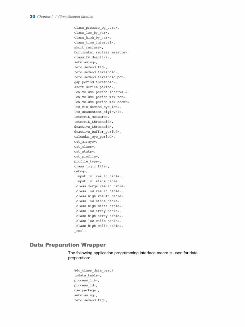
The following application programming interface macro is used for data preparation:
%dc_class_data_prep(indata_table=,process_lib=,process_id=,use_package=,setmissing=,zero_demand_flg=,
30 Chapter 2 / Classification Module

zero_demand_threshold=,zero_demand_threshold_pct=,gap_period_threshold=,short_series_period=,low_volume_period_interval=,low_volume_period_max_tot=,low_volume_period_max_occur=,lts_min_demand_cyc_len=,lts_seasontest_siglevel=,intermit_measure=,intermit_threshold=,deactive_threshold=,deactive_buffer_period=,calendar_cyc_period=,need_sort=,time_id_var=,demand_var=,input_vars=,lvl_by_vars=,class_time_interval=,out_arrays=,out_stats=,out_profile=,profile_type=,debug=,_scalar_table=,_array_table=,_calib_table=,_rc=);
Data Preparation Process
Process Flow
For the data preparation process, each time series is analyzed, and then the required statistics are computed.
The following data preparation process flow is implemented for each selected level in the hierarchy:
1 Aggregate the data to the desired level, based on BY variables and the time interval that is selected.
2 Identify the components of the time series.
3 Compute the requested statistics.
4 Make a classification decision.
Data Preparation Process 31

Algorithms for Classification
Preliminary Classification
The preliminary classification process is based on the following default classification logic:
If CLASSIFY_DEACTIVE and DEACTIVE_FLG=1=>DEACTIVEElse if _TOT_NOBS<=SHORT_SERIES_PERIOD=>SHORTElse if _PERIOD_COUNT=0or_PERIOD_DEMAND_TOT_MAX<=LOW_VOLUME_PERIOD_MAX_TOTALor_PERIOD_DEMAND_OCCUR_MAX<=LOW_VOLUME_PERIOD_MAX_OCCUR=>LOW VOLUMEElse if _DEMAND_CYC_LEN_COUNT>0If _DEMAND_CYC_LEN_MAX<=LTS_MIN_DEMAND_CYC_LENand _CURRENT_CYC_INDEX-_TRAILING_ZERO_LEN<=LTS_MIN_DEMAND_CYC_LEN=>STSElse =>LTSElse if _TRIM_NOBS> LTS_MIN_DEMAND_CYC_LEN =>LTSElse =>UNCLASSIFIABLE
If STSIf _INTERMIT_FLG=>STS_INTERMITElse =>STS_NON_INTERMIT
If LTSIf _INTERMIT_FLG=>LTS_INTERMITElse If _SEASONAL_FLG=1=>LTS_SEASONALElse If _SEASONAL_FLG=0=>LTS_NON_SEASONALElse =>LTS_UNCLASS
You can replace the default classification logic with a user-provided classification logic file, which must conform to the supported format as shown in the following image:
The file should contain a macro for the logic, and must call the macro at the end of the file. The logic macro should use the PROC TIMEDATA programming statement language to assign values to the column, _Dc_Prelim_By_N, which is converted to different classes at a later time. The values and corresponding classes are listed in the following table:
_Dc_Prelim_By_N Class
1 Short
32 Chapter 2 / Classification Module

_Dc_Prelim_By_N Class
2 Low_Volume
3 STS_Non_Intermit
4 STS_Intermit
5 LTS_Season
6 LTS_Non_Season
7 LTS_Intermit
8 LTS_Season_Intermit
9 LTS_Unclass
10 Unclass
11 LTS
12 STS
13 Deactive
The macro can use all the supported statistics and analytical parameters (as a macro variable) listed in the following table:
Algorithms for Classification 33
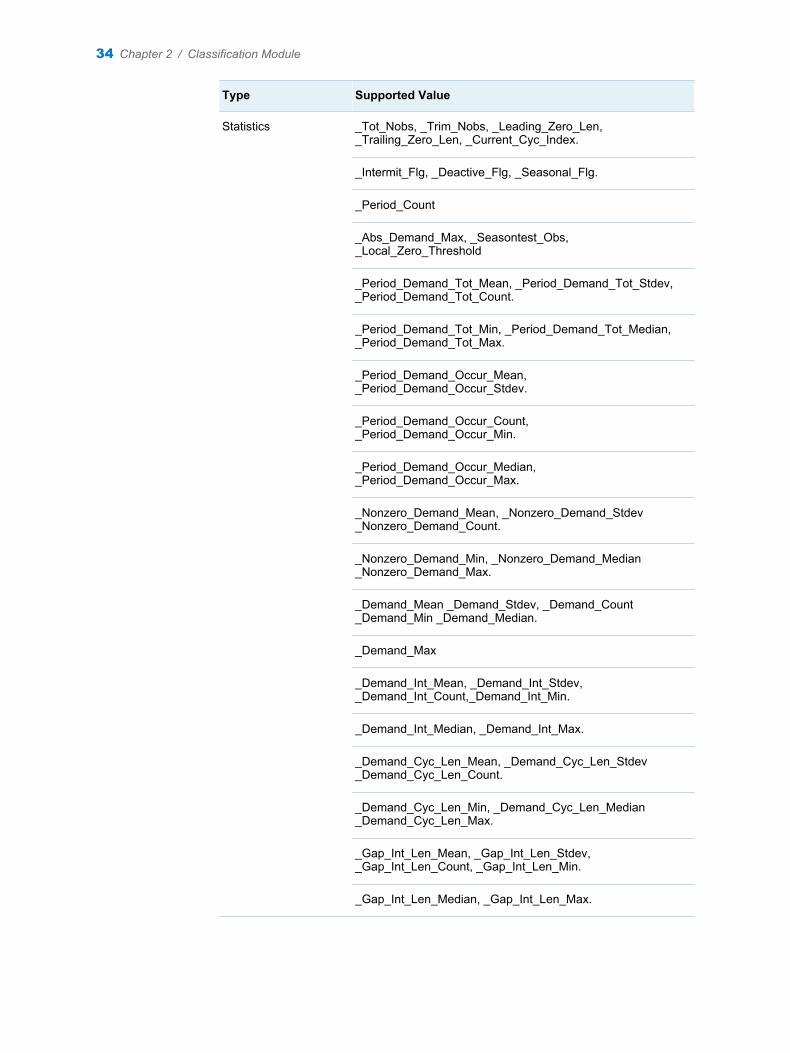
Type Supported Value
Statistics _Tot_Nobs, _Trim_Nobs, _Leading_Zero_Len, _Trailing_Zero_Len, _Current_Cyc_Index.
_Intermit_Flg, _Deactive_Flg, _Seasonal_Flg.
_Period_Count
_Abs_Demand_Max, _Seasontest_Obs, _Local_Zero_Threshold
_Period_Demand_Tot_Mean, _Period_Demand_Tot_Stdev, _Period_Demand_Tot_Count.
_Period_Demand_Tot_Min, _Period_Demand_Tot_Median, _Period_Demand_Tot_Max.
_Period_Demand_Occur_Mean, _Period_Demand_Occur_Stdev.
_Period_Demand_Occur_Count, _Period_Demand_Occur_Min.
_Period_Demand_Occur_Median, _Period_Demand_Occur_Max.
_Nonzero_Demand_Mean, _Nonzero_Demand_Stdev _Nonzero_Demand_Count.
_Nonzero_Demand_Min, _Nonzero_Demand_Median _Nonzero_Demand_Max.
_Demand_Mean _Demand_Stdev, _Demand_Count _Demand_Min _Demand_Median.
_Demand_Max
_Demand_Int_Mean, _Demand_Int_Stdev, _Demand_Int_Count,_Demand_Int_Min.
_Demand_Int_Median, _Demand_Int_Max.
_Demand_Cyc_Len_Mean, _Demand_Cyc_Len_Stdev _Demand_Cyc_Len_Count.
_Demand_Cyc_Len_Min, _Demand_Cyc_Len_Median _Demand_Cyc_Len_Max.
_Gap_Int_Len_Mean, _Gap_Int_Len_Stdev, _Gap_Int_Len_Count, _Gap_Int_Len_Min.
_Gap_Int_Len_Median, _Gap_Int_Len_Max.
34 Chapter 2 / Classification Module

Type Supported Value
Analytical Parameters &zero_demand_threshold
&zero_demand_flg
&zero_demand_threshold_pct
&gap_period_threshold
&short_series_period
&low_volume_period_interval
&low_volume_period_max_tot
&low_volume_period_max_occur
<s_min_demand_cyc_len
<s_seasontest_siglevel
&intermit_measure
&intermit_threshold
&deactive_threshold
&deactive_buffer_period
&calendar_cyc_period
Example of Default Classification Logic
The default classification logic can be written in the following way:
%macro dc_class_default_logic;_DC_PRELIM_BY_N = 10; /*UNCLASS*/if &classify_deactive; and _DEACTIVE_FLG=1then _DC_PRELIM_BY_N=13; /*DEACTIVE*/else if _TOT_NOBS<=&short_series_period;then _DC_PRELIM_BY_N = 1; /*SHORT*/else if _PERIOD_COUNT=0 or _PERIOD_DEMAND_TOT_MAX<=&low_volume_period_max_tot;or _PERIOD_DEMAND_OCCUR_MAX<=&low_volume_period_max_occur;then _DC_PRELIM_BY_N=2; /*LOW VOLUME*/else if _DEMAND_CYC_LEN_COUNT>0 then do;if _DEMAND_CYC_LEN_MAX<=<s_min_demand_cyc_len;and _CURRENT_CYC_INDEX-_TRAILING_ZERO_LEN<=<s_min_demand_cyc_len;then _DC_PRELIM_BY_N=12; /*STS*/else _DC_PRELIM_BY_N=11; /*LTS*/end;
Algorithms for Classification 35

else if _TRIM_NOBS><s_min_demand_cyc_len;then _DC_PRELIM_BY_N=11; /*LTS*/if _DC_PRELIM_BY_N=12 then do;if _INTERMIT_FLG=0then _DC_PRELIM_BY_N = 3; /*STS_NON_INTERMIT*/else if _INTERMIT_FLG=1then _DC_PRELIM_BY_N = 4; /*STS_INTERMIT*/end;else if _DC_PRELIM_BY_N=11 then do;if _INTERMIT_FLG=1then _DC_PRELIM_BY_N = 7; /*LTS_INTERMIT*/else if _SEASONAL_FLG=1then _DC_PRELIM_BY_N = 5; /*LTS_SEASON*/else if _SEASONAL_FLG=0then _DC_PRELIM_BY_N = 6; /*LTS_NON_SEASON*/else _DC_PRELIM_BY_N = 9; /*LTS_UNCLASS*/end;%if &syscc; > 4 %then %do; /* NO_COVERAGE */%put ERROR: in &SYSMACRONAME.; /*sasmsg*/%end;%mend dc_class_default_logic;
Horizontal Reclassification
The types Lts_Unclass, Unclass, and Short might be reclassified in the horizontal reclassification process. When the value of Horizontal_Relcass_Measure is None, the horizontal reclassification process is not initiated. When the value of Horizontal_Relcass_Measure is not None, the horizontal reclassification process is run and the following reclassification results are generated.
The Lts_Unclass type is reclassified into the following classes:
n Lts_Season
n Lts_Non_Season
The Unclass type is reclassified into of the following classes:
n Lts_Season
n Lts_Non_Season
n Lts_Intermit
n Sts_Intermit
n Sts_Non_Intermit
If the configuration setting Short_Reclass is turned on, then the Short type is reclassified into one of the following classes:
n Lts_Season
n Lts_Non_Season
n Lts_Intermit
n Sts_Intermit
n Sts_Non_Intermit
n Low_Volume
36 Chapter 2 / Classification Module

The Horizontal_Relcass_Measure configuration parameter also controls the measurement that is used to determine the reclassification results. The values for this configuration parameter are Mode or Max_Demand. If you specify Mode, then the preliminary classification results are analyzed to identify all the sibling time series under the same parent node. The class type follows the reclassification rule that occurs most often for the reclassification results, that is, for the intermediate classification result.
If you specify Max_Demand , then the total _Demand_Mean for the sibling series is computed with the same class type. The class type that follows the reclassification rule that has the largest Total _Demand_Mean for the reclassification result.
If there is a match in using the selected measures, the leftover measure is considered. For example, if mode is selected and two eligible class types occur equal number of times, the one with largest total _Demand_Mean is considered as the reclassification result.
The system searches for the reclassification results from all the sibling time series. If there are no qualified classification results (for example, there is no sibling times series classified as Lts_Non_Season or Lts_Season for a Lts_Unclass time series), then the system considers the nodes one level above the parent node, and looks for all sibling or cousin time series with the same grandparent node in the hierarchy. The procedure continues until a qualified reclassification result is found, or the system reaches the top level.
Top-down (Vertical) Reclassification
If the Class_High level is specified, then top-down reclassification might be performed. The reclassification is done at the Class_Low level, based on the intermediate classification results for both Class_Low and Class_High level. If the parent series at the Class_High level has been classified as LTS_Season, and the child series at the Class_Low level has been classified as LTS_Intermit, then the top-down reclassification process reclassifies the Class_Low level child series as LTS_Season_Intermit.
Modeling Strategy for Demand Classes
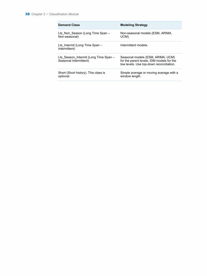
The following modeling strategies are recommended for these demand classes:
Demand Class Modeling Strategy
Low_Volume Simple average or moving average with a window length.
Sts_Non_Intermit (Short Time Span – Non-Intermittent)
Simple regression model with seasonal dummies.
Sts_Intermit (Short Time Span – Intermittent)
Simple regression model with seasonal dummies. IDM models for the in-season periods and 0 for other periods.
Lts_Season (Long Time Span – Seasonal)
Seasonal models (ESM, ARIMA, UCM).
Modeling Strategy for Demand Classes 37
Demand Class Modeling Strategy
Lts_Non_Season (Long Time Span – Non-seasonal)
Non-seasonal models (ESM, ARIMA, UCM).
Lts_Intermit (Long Time Span – Intermittent)
Intermittent models.
Lts_Season_Intermit (Long Time Span – Seasonal Intermittent)
Seasonal models (ESM, ARIMA, UCM) for the parent levels, IDM models for the low levels. Use top-down reconciliation.
Short (Short history). This class is optional.
Simple average or moving average with a window length.
38 Chapter 2 / Classification Module

3Pattern Clustering Module
Overview . . . . . . . . . . . . . . . . . . . . . . . . . . . . . . . . . . . . . . . . . . . . . . . . . . . . . . . . . . . . . . . . . . . 39
Approaches to Clustering . . . . . . . . . . . . . . . . . . . . . . . . . . . . . . . . . . . . . . . . . . . . . . . . . . . 39Overview . . . . . . . . . . . . . . . . . . . . . . . . . . . . . . . . . . . . . . . . . . . . . . . . . . . . . . . . . . . . . . . . 39Hierarchical Clustering Method . . . . . . . . . . . . . . . . . . . . . . . . . . . . . . . . . . . . . . . . . . . . 40K-means Clustering Method . . . . . . . . . . . . . . . . . . . . . . . . . . . . . . . . . . . . . . . . . . . . . . . 41Computing the Silhouette Coefficient . . . . . . . . . . . . . . . . . . . . . . . . . . . . . . . . . . . . . . . 42
Input and Output Parameters for Configuration . . . . . . . . . . . . . . . . . . . . . . . . . . . . . 43Input Data . . . . . . . . . . . . . . . . . . . . . . . . . . . . . . . . . . . . . . . . . . . . . . . . . . . . . . . . . . . . . . . 43Supported Output Results . . . . . . . . . . . . . . . . . . . . . . . . . . . . . . . . . . . . . . . . . . . . . . . . . 46
Macro for Application Programming Interface . . . . . . . . . . . . . . . . . . . . . . . . . . . . . . . 47
Overview
The pattern clustering module groups series with similar demand pattern together. This process helps build the forecast hierarchy and improves forecast accuracy.
For example, winter clothes and summer swimming suits are both products with short life span, but they have different demand patterns. Forecasting them together would result in forecast summer sales for winter clothes and winter sales for summer wear, such as swim suits, which is inaccurate. However, forecasting them separately ensures that the right seasons are considered.
Approaches to Clustering
Overview
The clustering process is used to group time series data with similar demand patterns into clusters. For example, winter apparel such as winter jackets and winter sweaters are both products that have peak sales in winter. Therefore, these products belong to the same cluster.
After the classification process is run, for each long time span seasonal and short time span class, demand series with similar patterns are clustered together. There are several techniques that you can use to cluster the time series. SAS Demand Classification and Clustering supports the following clustering methods:
39

n hierarchical clustering
n k-means clustering
Hierarchical Clustering Method
Overview
Hierarchical clustering is a method of cluster analysis that seeks to build a hierarchy of clusters. Strategies for hierarchical clustering are categorized into the following two types:
agglomerativeThis is a bottom-up approach. At the beginning of this method, each observation has its own cluster. Pairs of clusters are merged as you move up in the hierarchy.
divisiveThis is a top-down approach. All observations start in one cluster, and splits are performed recursively as you move down the hierarchy.
Hierarchical clustering has a distinct advantage, because any valid measure of distance can be used. The observations themselves are not required, only a matrix of distances is used. PROC CLUSTER is used for hierarchical clustering. The methods that are used by PROC CLUSTER are based on the agglomerative hierarchical clustering procedure.
Managing Cluster Dissimilarities
To determine which clusters should be combined (for agglomerative), or where a cluster should be split (for divisive), a measure of dissimilarity between sets of observations is required. In most methods of hierarchical clustering, an appropriate metric (a measure of distance between pairs of observations) and a linkage criterion that specifies the dissimilarity of sets as a function of the pairwise distances of observations in the sets are used.
Choosing a Metric for Clustering
Several metrics are commonly used in hierarchical clustering. Choosing an appropriate metric determines the shape of the clusters. Some elements in a cluster might be close to one another according to one distance metric, and farther away according to another metric.
For example, in a 2-dimensional space, the distance between the point (1,0) and the origin (0,0) is always 1, according to the commonly accepted norms. But the distance between the point (1,1) and the origin (0,0) can be 2 or 1, when you use the Manhattan distance metric, Euclidean distance metric, or maximum distance metric.
Linkage Criterion
A linkage criterion determines the distance between sets of observations as a function of the pairwise distances between observations. The following linkage methods are supported:
n average method
n centroid method
40 Chapter 3 / Pattern Clustering Module

n Ward’s method
The Hi_Cluster_Method input parameter determines which method is used.
Workflow for Hierarchical Clustering
The following workflow is implemented for hierarchical clustering:
1 Using the profile data as input, if Hi_Indistance_Flag = 1, then compute the distance matrix.
2 Either use the distance matrix (Hi_Indistance_Flag=1) or use the original profile data (Hi_Indistance_Flag=0). Then, execute PROC CLUSTER to generate the hierarchical clusters:
n Specify the number of clusters. You can specify the exact number of clusters by specifying the value for the Num_Of_Clusters parameter. You can also specify multiple clusters in a range by specifying the values for the Min_Num_Of_Cluster and Max_Num_Of_Cluster parameters.
n Automatically determine the range and number of clusters, based on the following statistics:
o pseudo-F statistic
o pseudo T-squared statistic
o cubic clustering criterion
o R-squared statistic
n If more than one range is given, then based on these statistics, select the one with largest silhouette coefficient as the range of clusters.
3 Compute the silhouette coefficient as the cluster quality measurement.
For more information about computing the silhouette coefficient, see “Computing the Silhouette Coefficient” on page 42.
K-means Clustering Method
Overview
K-means clustering is a quantitative approach to clustering. It measures certain features of the products. For example, suppose you are measuring the percentage of milk and or other components in a product. All products with a high percentage of milk would be grouped together. In general, there are n data points that have to be partitioned in k-clusters. The goal is to assign a cluster to each data point. The k-means clustering method aims to find the positions μi ,i=1...k of the clusters that minimize the distance from the data points to the cluster.
The main advantage of using the k-means clustering method is that it works quickly. However, this approach requires a pre-determined number of clusters. SAS Demand Classification and Clustering uses k-means clustering as the default method for pattern clustering. The optimal number of clusters is automatically determined by hierarchical clustering. For more information, see “Determining the Number of Clusters” on page 42.
Approaches to Clustering 41

Workflow for K-means Clustering
The Lloyd's algorithm, also known as the k-means algorithm, is used to implement the k-means clustering method. The following workflow is implemented:
1 Determine the number of clusters, that is, the value of k.
2 Initialize the center point of the clusters.
3 Assign the closest cluster to each data point.
4 Set the position of each cluster to the mean of all data points that belong to that cluster.
5 Repeat steps two and three until convergence is achieved.
The algorithm eventually converges to a point, although it is not necessarily the minimum of the sum of squares. That is because the problem is non-convex, and the algorithm is just a heuristic, converging to a local minimum. The algorithm stops when the assignments do not change from one iteration to the next.
Determining the Number of Clusters
The number of clusters should match the data. An incorrect choice of the number of clusters invalidates the entire process. Hierarchical clustering is used to determine the optimal number of clusters. Use the following process to determine the number of clusters that you need:
1 Run k-means (PROC FASTCLUS) with the Max_Num_Of_Cluster parameter to generate the initial clusters.
2 Run hierarchical clustering on the initial cluster centers, and determine the optimal number of clusters. (You generated the initial cluster centers in Step 1.)
3 Run k-means clustering again on the original data set with the optimal number of clusters, which was determined in Step 2.
Computing the Silhouette Coefficient
Assume that the data has been clustered by using any technique, such as k-means, into clusters. For each datum i, assume that a (i) is the average dissimilarity of i with all other data within the same cluster. You can use any measure of dissimilarity, but distance measures are the most common.
You can interpret a (i) in terms of how i is suitable for the cluster that it is assigned to. The smaller the value, the better the suitability. Next, find the average dissimilarity of with the data of another single cluster. Repeat this for every cluster of which i is not a member. Denote the lowest average dissimilarity to i of any such cluster by b (i). The cluster with this lowest average dissimilarity is said to be the neighboring cluster of i as it is. Aside from the cluster that i is assigned, it is the cluster in which i fits best. It is computed as follows:
s ( i ) = b (i) − a (i)max { a (i), b (i) }
The above equation can also be expressed as follows:
42 Chapter 3 / Pattern Clustering Module

s ( i) = { 1 − a (i) / b (i), if a (i) < b (i)0, if a (i) = b (i)
b (i) / a (i) − 1, if a (i) > b (i)}
Therefore, − 1 ≤ s (i) ≤ 1
In order for s (i) to be close to 1, the following must be true:
a a ( i )≪ b ( i )
Because a (i) is a measure of how dissimilar i is to its own cluster, a small value means it is well suited. In addition, a large value of b (i) indicates that i is badly suited to its neighboring cluster.
If the value of s (i) is close to 1, the datum is appropriately clustered. If s (i) is close to –1, then it is more appropriate to clusteri in its neighboring cluster. If the value of s (i) is close to 0, then the datum is on the border of the two natural clusters.
The average s (i) of the overall data is a measure of how tightly grouped the data is in the cluster. Thus, the average s (i) of the overall data in the data set is a measure of how appropriately the data is clustered. If there are too many or too few clusters, as might occur when a poor choice of k is used in the k-means algorithm, then some of the clusters might most often display narrower silhouettes than the others. In this way, silhouette plots and averages are used to determine the natural number of clusters within a data set.
Input and Output Parameters for Configuration
Input Data
Input Parameters for Hierarchy Configuration
The following input parameters are supported for hierarchy configuration:
Parameter Name Description
Indata_Table Specifies the input data.
Process_Lib Specifies the temporary library.
Input Parameters for Process Configuration
The following input parameters are supported for process configuration:
Parameter Name Description
Need_Sort Flag that indicates whether a sort functionality is needed.
Input and Output Parameters for Configuration 43

Parameter Name Description
Cluster_Process_By_Vars Variables used for BY-group processin
Transpose_Flag Flag that indicates whether the input table needs to be tranposed.
Id_Vars Observations ID variables.
Profile_Vars A single variable or a set of variables that represent the profile. If the value of Transpose_Flag = 1, then a single variable is parsed, which represents the profile (for example, sales average). If the value of Transpose_Flag = 0, then a set of variables is parsed, which represent the profile (for example, month1, month2, and so on till month12).
Profile_Id_Vars This value is required if the value of Transpose_Flag = 1. An ID variable is parsed to identify each profile input (the month of the year, the week of the year, and so on).
Input Parameters for a Hierarchical Clustering Configuration
The following parameters are supported for a hierarchical clustering configuration:
Parameter Name Description
Hi_Distance_Measure Specifies the distance measure for the hierarchical clustering . Possible values are: Euclid, Disratio, Nonmetric, Canberra, Doverlap, Chisq, Chi, Phisq, Phi, Skldiv, Lamdbadiv, and Jsdiv. The default value is Skldiv.
Hi_Indistance_Flag Specifies whether to use distance matrix as input for hierarchical clustering. Possible values are 0 or 1. The default value is 0.
Cluster_Weight Specifies whether to include weight in the _Distance_Measure_Table.
Hi_Cluster_Method PROC CLUSTER is used for hierarchical clustering. Possible values are: Average, Centroid, and Ward.
44 Chapter 3 / Pattern Clustering Module

Parameter Name Description
Num_Of_Clusters Specifies the number of clusters. Possible values are: Auto or a user-specified number. However, if you specify a value for this parameter, then the Min_Num_Of_Clusters and Max_Num_Of_Clusters parameters are ignored.
Min_Num_Of_Clusters Specifies the minimum number of clusters, when Num_Of_Clusters = Auto. The default value is 1.
Max_Num_Of_Clusters Specifies the maximum number of clusters, when Num_Of_Clusters = Auto. The default value is 40.
Hi_Nosquare This is a PROC CLUSTER option. It is used to specify the value of square, either 0 or 1.
Ccc_Cutoff Specifies the cutoff value for the cubic clustering criteria that is used to determine the number of clusters. This parameter is applicable only when Num_Of_Clusters = Auto. The default value is 3.
Hi_Ncl_Selection Criteria for selecting the number of clusters. Possible values are: 1, 2, 3, 4, 5, and 6.
Hi_Rsq_Changerate Specifies the R-squared rate of change for detecting the number of clusters. Possible values are in the range 0–1. The default value is 0.1.
Hi_Rsq_Min Specifies the minimum R-square of the corresponding number of clusters to be considered. This parameter applies only when Hi_Ncl_Selection = 6 (R-squared method). Possible values are in the range 0–1. The default value is 0.99.
Hi_Rsq_Method Specifies which R-square-based method to use to determine the optimal number of clusters from the hierarchical cluster result. Possible values are Knee_S, Auto, and Backscan. The default value is Knee_S.
Hi_Rsq_Modelcomplexity Specifies the model complexity. Possible values are 0 or 1. The default value is 1.
Input and Output Parameters for Configuration 45

Parameter Name Description
Ncl_Cutoff_Pct_1 Specifies the cutoff percentage for the I2A_flag. To calculate, regress R-square on the number of clusters and pick the cluster number with maximum positive residual (number of clusters considered = 10 % of the number of observations). Possible values are in the range 0–1. Default value is 0.1.
Ncl_Cutoff_Pct_2 Specifies the cutoff percentage for the I2B_flag. To calculate, regress R-square on the number of clusters and pick the cluster number with maximum positive residual (number of clusters considered = 20 % of the number of observations). Possible values are in the range 0–1. Default value is 0.1.
Input Parameters for a K-Means Clustering Configuration
The following parameters are supported for a k-means clustering configuration:
Parameter Name Description
Km_Nomiss Specifies whether to turn on the Nomiss option for PROC FASTCLUS.
Km_Std Specifies the STD= option in PROC FASTCLUS.
Supported Output Results
The following results are supported:
n cluster results
o BY variables to identify series
o Pc_By (Cluster_Id)
n (optional) _Ncl_Range_Table (cluster range that is determined by hierarchical clustering)
n (optional)_Distance_Matrix_Table
n (optional)_Cluster_Quality_Table (silhouette coefficient)
Note: The silhouette coefficient is computed only when the number of series is less than 3000. If the number of series exceeds 3000, the silhouette coefficient is not computed due to memory considerations. A warning message is displayed in the log. The default value for the silhouette coefficient is 0.
46 Chapter 3 / Pattern Clustering Module

Macro for Application Programming Interface
The following application programming interface macro is used to execute the pattern clustering process:
%dc_cluster_wrapper(process_lib =work,indata_table = ,transpose_flag=0,id_vars =,profile_vars=,profile_id_var=,cluster_process_by_vars=,clustering_method=,hi_indistance_flag=,hi_distance_measure=,cluster_weight=0,hi_cluster_method =,num_of_clusters =AUTO,min_num_of_cluster=1,max_num_of_cluster=40,hi_nosquare =,hi_trim_p =,ncl_cutoff_pct_1 =0.1,ncl_cutoff_pct_2 =0.2,ccc_cutoff =3,hi_rsq_min =0.99,hi_rsq_method =KNEE,hi_rsq_changerate =0.1,hi_rsq_modelcomplexity =1,hi_ncl_selection=6,hi_max_obs_threshold=15000, /*hidden spec: always use KMEANS if the number of observations > 15000 to avoid performance issue in PROC CLUSTER*/km_nomiss =,km_std =,_cluster_result_table =,_ncl_range_table =,_cluster_quality_table =,debug = 0,_rc =);
Macro for Application Programming Interface 47

48 Chapter 3 / Pattern Clustering Module
4Volume Grouping Module
Overview . . . . . . . . . . . . . . . . . . . . . . . . . . . . . . . . . . . . . . . . . . . . . . . . . . . . . . . . . . . . . . . . . . . 49
The Volume Grouping Process . . . . . . . . . . . . . . . . . . . . . . . . . . . . . . . . . . . . . . . . . . . . . 49
Approaches to Volume Grouping . . . . . . . . . . . . . . . . . . . . . . . . . . . . . . . . . . . . . . . . . . . 50Overview . . . . . . . . . . . . . . . . . . . . . . . . . . . . . . . . . . . . . . . . . . . . . . . . . . . . . . . . . . . . . . . . 50Dynamic Grouping . . . . . . . . . . . . . . . . . . . . . . . . . . . . . . . . . . . . . . . . . . . . . . . . . . . . . . . . 50Dynamic Grouping with Hierarchy Restriction . . . . . . . . . . . . . . . . . . . . . . . . . . . . . . . 53Post-processing Results . . . . . . . . . . . . . . . . . . . . . . . . . . . . . . . . . . . . . . . . . . . . . . . . . . 56
Input and Output Parameters for Configuration . . . . . . . . . . . . . . . . . . . . . . . . . . . . . 57Input Parameters for Process Configuration . . . . . . . . . . . . . . . . . . . . . . . . . . . . . . . . 57Supported Output Results . . . . . . . . . . . . . . . . . . . . . . . . . . . . . . . . . . . . . . . . . . . . . . . . . 59
Macro for Application Programming Interface . . . . . . . . . . . . . . . . . . . . . . . . . . . . . . . 59
Overview
Demand forecasting for lower levels in the hierarchy might skew statistical forecasts due to insufficient demand volume and large random variation. If there is a sufficient volume of data, you can generate reliable forecasts by using forecasting models. Volume grouping is used to aggregate sales and minimize random variation in data. By aggregating sales, stronger underlying demand signals can be generated. This makes demand patterns easier to analyze.
The volume grouping module enables you to determine the forecast reconciliation level that ensures that the forecasts are generated at a level with sufficient demand volume. Volume grouping also ensures that demand patterns specific to each demand series are retained as far as possible.
The Volume Grouping Process
Volume groups are generated based on the user-specified volume threshold, which is based on the demand average. You can define a level in the hierarchy as the lowest grouping level, below which the hierarchy is unbreakable. All nodes below the lowest grouping level that belong to the same hierarchy node are clustered in the same segment. The aggregated sales volume at each node is compared with the volume threshold. Starting from the lowest grouping level, if a series has sufficient volume, then the forecast is done at the same level to capture any series-specific patterns. Otherwise, the series is aggregated to one
49

level higher with other low volume series until the series reaches a level with sufficient volume, or it reaches the top level.
Volume groups are generated within the scope that is defined by demand classification and pattern clustering, depending on which components you are running. The process of volume grouping can be run stand-alone, or after you have completed the classification and pattern clustering processes. Forecasts are generated at the volume group level and are then disaggregated down to the lowest level.
Approaches to Volume Grouping
Overview
SAS Demand Classification and Clustering supports two hierarchy-based methods for volume grouping:
n dynamic grouping
n dynamic grouping with hierarchy restriction
Dynamic Grouping
In this method, two parameters are defined as the volume threshold: Avg_Demand_Threshold and Min_Frequency_Threshold. If the average demand of an aggregated series is greater than or equal to the Avg_Demand_Threshold, and the number of demand occurrences is greater than or equal to the Min_Frequency_Threshold, then the series is considered to have sufficient volume.
If a series at a lower level has sufficient volume, then the forecast is done at the same level to capture any series-specific patterns. Otherwise, the series is aggregated to one level higher with other low volume series until the series reaches a level with sufficient volume, or it reaches the top level.
The following figure shows the hierarchy of a data set, where volume grouping is to be implemented. The low level is the lowest level of the hierarchy. The lowest grouping level is the user-defined low level for volume grouping.
50 Chapter 4 / Volume Grouping Module

Figure 4.1 Hierarchy of Data for Volume Grouping
First the series is aggregated up to the lowest grouping level. The series is compared with the demand volume (that is, the average demand and demand occurrences of each node) to determine whether it passes the threshold.
Figure 4.2 Lowest Grouping Level
A green node indicates a node that has sufficient volume and that passes the volume threshold. A red node indicates a low-volume node, which does not have sufficient volume to pass the threshold.
In the next step, all the nodes with insufficient volume are aggregated up one level. In this example, node B1 is aggregated with node B2. Node B8 is aggregated with node B9. However, the aggregated node B8+B9 still has insufficient volume. Nodes B3 and B6 move up one level independently. The
Approaches to Volume Grouping 51

figure shows the status of each node at the corresponding level: After aggregation, nodes B1 and B2 have sufficient volume, but the remaining nodes must be aggregated up one more level.
Figure 4.3 Aggregated Nodes
The process is repeated until all the nodes satisfy the volume thresholds, or until the nodes reach the top level.
Figure 4.4 Aggregated Nodes at Top Level
In the example given in the Figure 4.4 on page 52, by using dynamic grouping, you get six groups. Five of these groups pass the volume threshold. Node B3 becomes a low-volume cluster because it reaches the top level.
52 Chapter 4 / Volume Grouping Module

Figure 4.5 Dynamic Grouping Final Outcome
Dynamic Grouping with Hierarchy Restriction
In the example provided in “Dynamic Grouping” on page 50, the grouping results do not retain the integrity of the original hierarchy structure. For example, nodes B5, B6, and B7 are not in the same group, although they are under the same parent node. Sometimes you might want to retain the integrity of the original hierarchy for special cases, such as when there are cross effects within a branch. If you add some hierarchy restrictions when the dynamic grouping is implemented, then you can preserve the integrity of the original hierarchy. The following figure shows the hierarchy of a data set, where volume grouping is to be implemented. The low level is the lowest level of the hierarchy. The lowest grouping level is the user-defined low level for volume grouping.
Figure 4.6 Hierarchy of Data for Volume Grouping
Approaches to Volume Grouping 53

In this approach, if a series at a lower level has sufficient volume, but one or more of its siblings do not have sufficient volume, then all nodes with the same parent are aggregated up. This method of aggregation retains the original hierarchy. A node finds its group if all sibling nodes have sufficient volume.
Figure 4.7 Lowest Grouping Level
A green node indicates a cluster that passes the volume threshold (a qualified node). A red node indicates a low-volume node, which does not pass the threshold (an unqualified node).
At the current level in the hierarchy, each parent node is checked. The level of qualified nodes is the current level. If all children under a parent node are qualified nodes, then all qualified nodes form their own cluster. If there are any unqualified nodes under a parent node, then all children nodes (under the same parent node) are aggregated up to the parent node.
Nodes B4, B5, and B7 are qualified nodes, but all of them have unqualified siblings. Therefore, all nodes are aggregated up one additional level.
54 Chapter 4 / Volume Grouping Module

Figure 4.8 Aggregated Nodes
Node B5+B6+B7 is a qualified node. However, its sibling node B8+B9 is still unqualified. Nodes with sufficient and significant demand volume might still need to aggregate up because one or two nodes do not satisfy the volume criteria. Therefore, node B8+B9 must be aggregated further up, until all siblings are qualified nodes.
Figure 4.9 Aggregated Nodes at Top Level
The final outcome is established with three volume groups and two reconciliation levels.
Approaches to Volume Grouping 55

Figure 4.10 Dynamic Grouping with Hierarchy Restriction Final Outcome
In the example given in the Figure 4.10 on page 56, by using dynamic grouping with the restricted hierarchy approach, you get three groups. This approach is similar to the flexible grouping method, except that the integrity of the branches in the hierarchy is intact.
In some cases, nodes with sufficient and significant demand volume need to aggregate up simply because one or two nodes do not satisfy the volume criteria. In this case, a node with insufficient volume might benefit from the aggregation. However, nodes with maximum demand do not benefit much from the aggregation, or such nodes might get some noise from the aggregation. Therefore, you might want to add some trade-off criteria to determine whether to take the grouping process up one level or to stay at the current level.
The following trade-off criteria are recommended:
1 If the Unqualified_Volume_Percentage value is greater than or equal to the Min_Unqualified_Volume_Pct value, then go up one level.
2 If the Unqualified_Node_Count_Percentage value is greater than or equal to the Min_ Unqualified_Node_Count_Pct value, then go up one level.
3 Otherwise, stay at the current level.
Post-processing Results
After the volume grouping process is complete, each item is assigned to a group and the grouping information is stored in the metadata table. During post-processing, the grouping information is remerged with the original data so that the final output contains all the original information and an additional column, Vg_By. If some items are completely filtered out while data is prepared during post-processing, then _Top_ is assigned as the Vg_By value for those filtered items. If BY variables are specified, a negative _Group_Id with values starting from -1 is assigned for each BY group.
56 Chapter 4 / Volume Grouping Module

Input and Output Parameters for Configuration
Input Parameters for Process Configuration
The following input parameters are used for process configuration:
Parameter Name Description
Process_Lib Specifies the library for processing temporary data and output. The default value is work.
Indata_Table Specifies the input data.
Need_Sort Flag that specifies whether the Indata_Table needs to be sorted by all BY variables that identify Class_Low level. Possible values are 0 and 1. Default value is 1.
Demand_Var This variable records the demand. It contains character values.
Time_Id_Var This variable represents the time ID. It contains character and numeric values.
Group_Time_Interval Specifies the frequency of the accumulated time series. The accumulation method is total. For possible values, see PROC TIMEDATA documentation.
Hier_By_Vars BY variables in a specific order, which represent the hierarchy.
Group_Process_By_Vars Variables that are used for BY processing.
Setmissing The value for the setmissing argument in the ID statement in PROC TIMEDATA. The default value is 0. For possible values, see PROC TIMEDATA documentation. This is a common input parameter that is shared by the demand classification and volume grouping modules.
Input and Output Parameters for Configuration 57
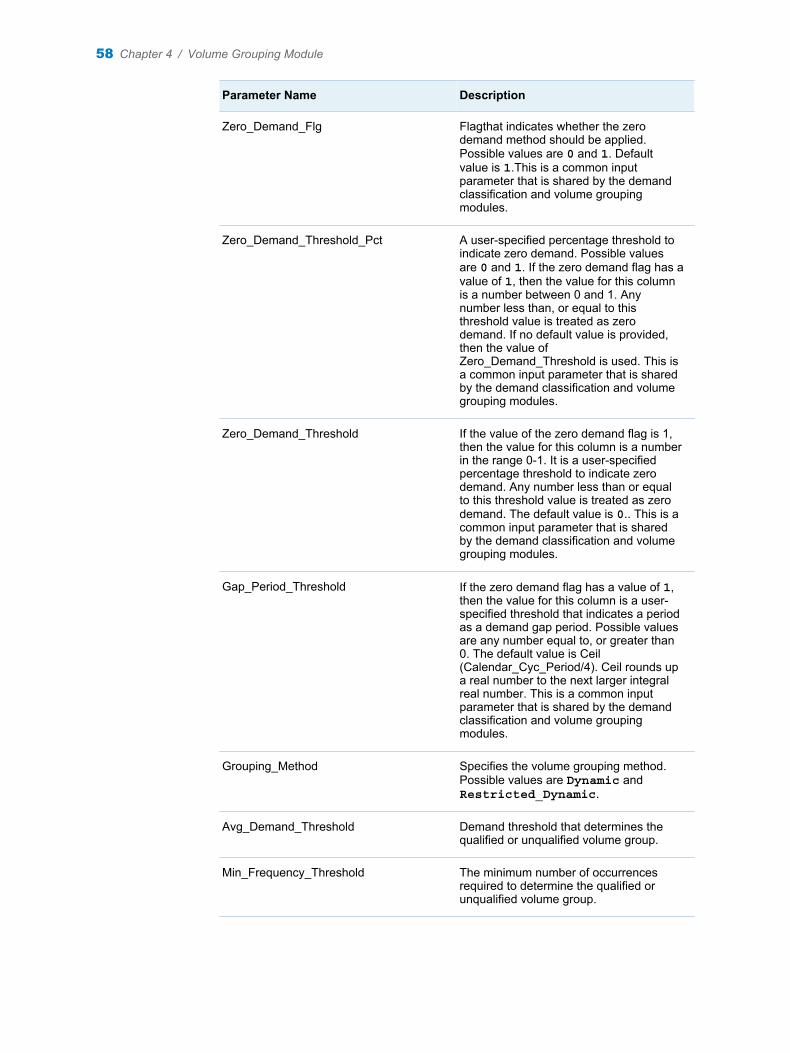
Parameter Name Description
Zero_Demand_Flg Flagthat indicates whether the zero demand method should be applied. Possible values are 0 and 1. Default value is 1.This is a common input parameter that is shared by the demand classification and volume grouping modules.
Zero_Demand_Threshold_Pct A user-specified percentage threshold to indicate zero demand. Possible values are 0 and 1. If the zero demand flag has a value of 1, then the value for this column is a number between 0 and 1. Any number less than, or equal to this threshold value is treated as zero demand. If no default value is provided, then the value of Zero_Demand_Threshold is used. This is a common input parameter that is shared by the demand classification and volume grouping modules.
Zero_Demand_Threshold If the value of the zero demand flag is 1, then the value for this column is a number in the range 0-1. It is a user-specified percentage threshold to indicate zero demand. Any number less than or equal to this threshold value is treated as zero demand. The default value is 0.. This is a common input parameter that is shared by the demand classification and volume grouping modules.
Gap_Period_Threshold If the zero demand flag has a value of 1, then the value for this column is a user-specified threshold that indicates a period as a demand gap period. Possible values are any number equal to, or greater than 0. The default value is Ceil (Calendar_Cyc_Period/4). Ceil rounds up a real number to the next larger integral real number. This is a common input parameter that is shared by the demand classification and volume grouping modules.
Grouping_Method Specifies the volume grouping method. Possible values are Dynamic and Restricted_Dynamic.
Avg_Demand_Threshold Demand threshold that determines the qualified or unqualified volume group.
Min_Frequency_Threshold The minimum number of occurrences required to determine the qualified or unqualified volume group.
58 Chapter 4 / Volume Grouping Module
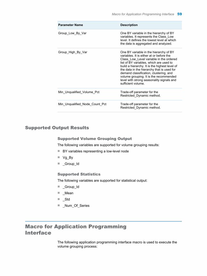
Parameter Name Description
Group_Low_By_Var One BY variable in the hierarchy of BY variables. It represents the Class_Low level. It defines the lowest level at which the data is aggregated and analyzed.
Group_High_By_Var One BY variable in the hierarchy of BY variables. It is either at or before the Class_Low_Level variable in the ordered list of BY variables, which are used to build a hierarchy. It is the highest level of the data in the hierarchy that is used for demand classification, clustering, and volume grouping. It is the recommended level with strong seasonality signals and sufficient volume.
Min_Unqualified_Volume_Pct Trade-off parameter for the Restricted_Dynamic method.
Min_Unqualified_Node_Count_Pct Trade-off parameter for the Restricted_Dynamic method.
Supported Output Results
Supported Volume Grouping Output
The following variables are supported for volume grouping results:
n BY variables representing a low-level node
n Vg_By
n _Group_Id
Supported Statistics
The following variables are supported for statistical output:
n _Group_Id
n _Mean
n _Std
n _Num_Of_Series
Macro for Application Programming Interface
The following application programming interface macro is used to execute the volume grouping process:
Macro for Application Programming Interface 59

%dc_vg_wrapper(process_lib=,need_sort=1,indata_table=,demand_var=,time_id_var=,group_time_interval=,group_process_by_vars=,hier_by_vars=,grouping_method=DYNAMIC,group_low_by_var=,group_high_by_var=, setmissing=,zero_demand_flg=1,zero_demand_threshold_pct=,zero_demand_threshold=,gap_period_threshold=,avg_demand_threshold=,min_frequency_threshold=,min_unqualified_volume_pct=,min_unqualified_node_count_pct=,vg_by_var_length=32,_vg_result_table=,_vg_statistics_table=,_vg_merged_table=,debug=0,_rc=)
60 Chapter 4 / Volume Grouping Module

5Segmenting Demand
Overview of Demand Segmentation . . . . . . . . . . . . . . . . . . . . . . . . . . . . . . . . . . . . . . . . . 61
Input and Output Parameters for Configuration . . . . . . . . . . . . . . . . . . . . . . . . . . . . . 61Input Parameters for General Configuration . . . . . . . . . . . . . . . . . . . . . . . . . . . . . . . . 61Input Parameters for Demand Classification . . . . . . . . . . . . . . . . . . . . . . . . . . . . . . . . 65Input Parameters for Pattern Clustering . . . . . . . . . . . . . . . . . . . . . . . . . . . . . . . . . . . . 66Input Parameters for Volume Grouping . . . . . . . . . . . . . . . . . . . . . . . . . . . . . . . . . . . . . 66Input Parameters for Output Configuration . . . . . . . . . . . . . . . . . . . . . . . . . . . . . . . . . . 67
Workflow for Segmentation . . . . . . . . . . . . . . . . . . . . . . . . . . . . . . . . . . . . . . . . . . . . . . . . . 67
Example of the Demand Segmentation Process . . . . . . . . . . . . . . . . . . . . . . . . . . . . . 68Example Input Data . . . . . . . . . . . . . . . . . . . . . . . . . . . . . . . . . . . . . . . . . . . . . . . . . . . . . . . 68General Configuration . . . . . . . . . . . . . . . . . . . . . . . . . . . . . . . . . . . . . . . . . . . . . . . . . . . . 69Classification Process . . . . . . . . . . . . . . . . . . . . . . . . . . . . . . . . . . . . . . . . . . . . . . . . . . . . 69Pattern Clustering Process . . . . . . . . . . . . . . . . . . . . . . . . . . . . . . . . . . . . . . . . . . . . . . . . 70Volume Grouping Process . . . . . . . . . . . . . . . . . . . . . . . . . . . . . . . . . . . . . . . . . . . . . . . . 71Job Output . . . . . . . . . . . . . . . . . . . . . . . . . . . . . . . . . . . . . . . . . . . . . . . . . . . . . . . . . . . . . . . 71
Code Structure for Segmentation . . . . . . . . . . . . . . . . . . . . . . . . . . . . . . . . . . . . . . . . . . . 72
Macro for Application Programming Interface . . . . . . . . . . . . . . . . . . . . . . . . . . . . . . . 72
Overview of Demand Segmentation
Demand segmentation integrates the classification, pattern clustering, and volume grouping processes by using the %dc_job macro. This integrated approach enables you to run all three modules together. Based on the outcome, you can select and apply suitable modeling techniques and forecasting strategies for each demand segment.
Input and Output Parameters for Configuration
Input Parameters for General Configuration
The %dc_job macro supports the following input parameters:
61

Parameter Name Description
Process_Lib Specifies the library for processing temporary data and output. The default value is work.
Use_Package Flag that indicates whether the Time Series Analysis (TSA) package for PROC TIMEDATA should be used. Possible values are 0 and 1. Default value is 0.
Note: Using this package might enhance performance. However , it requires the second maintenance release or later of SAS 9.4.
Need_Sort Flag that indicates whether the Indata_Table needs to be sorted by all BY variables that identify Class_Low level. Possible values are 0 or 1. Default value is 1.
Indata_Table Specifies the input data.
Time_Id_Var This variable represents the time ID. It contains character and numeric values.
Demand_Var This variable records the demand. It contains character values.
Hier_By_Vars BY variables in a specific order, which represent the hierarchy.
Process_By_Var Variables that are used for BY processing.
Low_By_Var One BY variable in the hierarchy of BY variables. It specifies the lowest level at which the data is aggregated and analyzed. It is the level at which the profiles for pattern clustering are computed. Corresponding input parameters (Class_Low_By_Var and Group_Low_By_Var) are supported for the demand classification and volume grouping modules.
62 Chapter 5 / Segmenting Demand
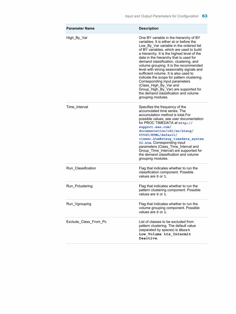
Parameter Name Description
High_By_Var One BY variable in the hierarchy of BY variables. It is either at or before the Low_By_Var variable in the ordered list of BY variables, which are used to build a hierarchy. It is the highest level of the data in the hierarchy that is used for demand classification, clustering, and volume grouping. It is the recommended level with strong seasonality signals and sufficient volume. It is also used to indicate the scope for pattern clustering. Corresponding input parameters (Class_High_By_Var and Group_High_By_Var) are supported for the demand classification and volume grouping modules.
Time_Interval Specifies the frequency of the accumulated time series. The accumulation method is total.For possible values, see user documentation for PROC TIMEDATA at http://support.sas.com/documentation/cdl/en/etsug/65545/HTML/default/viewer.htm#etsug_timedata_syntax02.htm. Corresponding input parameters (Class_Time_Interval and Group_Time_Interval) are supported for the demand classification and volume grouping modules.
Run_Classification Flag that indicates whether to run the classification component. Possible values are 0 or 1.
Run_Pclustering Flag that indicates whether to run the pattern clustering component. Possible values are 0 or 1.
Run_Vgrouping Flag that indicates whether to run the volume grouping component. Possible values are 0 or 1.
Exclude_Class_From_Pc List of classes to be excluded from pattern clustering. The default value (separated by spaces) is Short Low_Volume Lts_Intermit Deactive.
Input and Output Parameters for Configuration 63
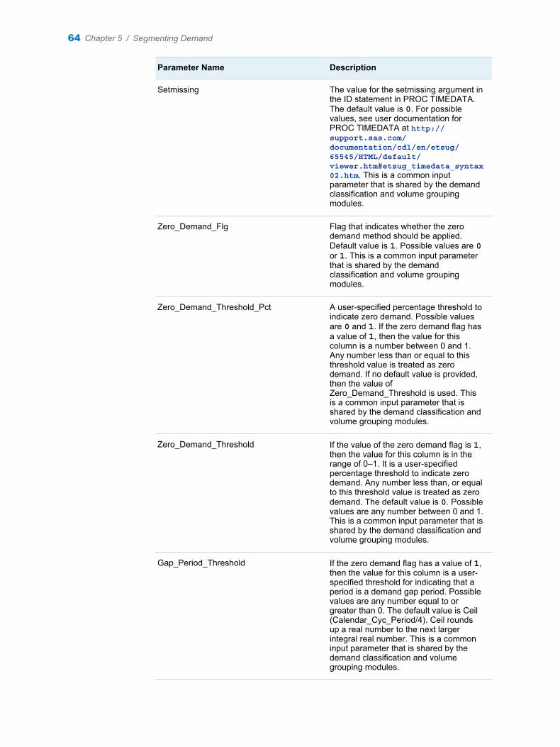
Parameter Name Description
Setmissing The value for the setmissing argument in the ID statement in PROC TIMEDATA. The default value is 0. For possible values, see user documentation for PROC TIMEDATA at http://support.sas.com/documentation/cdl/en/etsug/65545/HTML/default/viewer.htm#etsug_timedata_syntax02.htm. This is a common input parameter that is shared by the demand classification and volume grouping modules.
Zero_Demand_Flg Flag that indicates whether the zero demand method should be applied. Default value is 1. Possible values are 0 or 1. This is a common input parameter that is shared by the demand classification and volume grouping modules.
Zero_Demand_Threshold_Pct A user-specified percentage threshold to indicate zero demand. Possible values are 0 and 1. If the zero demand flag has a value of 1, then the value for this column is a number between 0 and 1. Any number less than or equal to this threshold value is treated as zero demand. If no default value is provided, then the value of Zero_Demand_Threshold is used. This is a common input parameter that is shared by the demand classification and volume grouping modules.
Zero_Demand_Threshold If the value of the zero demand flag is 1, then the value for this column is in the range of 0–1. It is a user-specified percentage threshold to indicate zero demand. Any number less than, or equal to this threshold value is treated as zero demand. The default value is 0. Possible values are any number between 0 and 1. This is a common input parameter that is shared by the demand classification and volume grouping modules.
Gap_Period_Threshold If the zero demand flag has a value of 1, then the value for this column is a user-specified threshold for indicating that a period is a demand gap period. Possible values are any number equal to or greater than 0. The default value is Ceil (Calendar_Cyc_Period/4). Ceil rounds up a real number to the next larger integral real number. This is a common input parameter that is shared by the demand classification and volume grouping modules.
64 Chapter 5 / Segmenting Demand

Parameter Name Description
_Job_Meta_Res_Table Metadata result table for all selected components. Either the Job_Meta_Res_Table or the _Job_Merge_Res_Table should be specified.
_Job_Merge_Res_Table This table merges the input tables with the results for all the selected components. The default is %process_lib..job_merge_res if _Job_Meta_Res_Table and _Job_Merge_Res_Table are not specified.
Input Parameters for Demand Classification
The %dc_job macro supports the following parameters for demand classification:
n Class_Input_Vars
n Short_Reclass
n Horizontal_Reclass_Measure
n Reclassify_Deactive
n Short_Series_Period
n Low_Volume_Period_Interval
n Low_Volume_Period_Max_Tot
n Low_Volume_Period_Max_Occur
n Lts_Min_Demand_Cyc_Len
n Lts_Seasontest_Siglevel
n Intermit_Measure
n Intermit_Threshold
n Deactive_Buffer_Period
n Calendar_Cyc_Period
n Current_Date
n Out_Class
n Out_Stats
n Out_Profile
n Profile_Type
n Class_Logic_File
Note: For descriptions of parameters related to the demand classification module, see “Input and Output Parameters for Configuration” on page 19.
Input and Output Parameters for Configuration 65

Input Parameters for Pattern Clustering
The %dc_job macro supports the following parameters for pattern clustering:
n Clustering_Method
n Hi_Indistance_Flag
n Hi_Distance_Measure
n Cluster_Weight
n Hi_Cluster_Method
n Num_Of_Clusters
n Min_Num_Of_Cluster
n Max_Num_Of_Cluster
n Hi_Nosquare
n Ncl_Cutoff_Pct_1
n Ncl_Cutoff_Pct_2
n Ccc_Cutoff
n Hi_Rsq_Min
n Hi_Rsq_Method
n Hi_Rsq_Changerate
n Hi_Rsq_Modelcomplexity
n Hi_Ncl_Selection
n Km_Nomiss
n Km_Std
Note: For descriptions of parameters related to the pattern clustering module, see “Input and Output Parameters for Configuration” on page 43.
Input Parameters for Volume Grouping
The %dc_job macro supports the following parameters for volume grouping:
n Grouping_Method
n Avg_Demand_Threshold
n Min_Frequency_Threshold
n Min_Unqualified_Volume_Pct
n Min_Unqualified_Node_Count_Pct
n Vg_By_Var_Length
Note: For descriptions of parameters related to the volume grouping module, see “Input and Output Parameters for Configuration” on page 57.
66 Chapter 5 / Segmenting Demand

Input Parameters for Output Configuration
The %dc_job macro supports the following parameters for output configuration:
n _Class_Result_Table
n _Class_Statistics_Table
n _Cluster_Result_Table
n _Cluster_Quality_Table
n _Vg_Result_Table
n _Vg_Statistics_Table
n _Job_Meta_Res_Table
n _Job_Merge_Res_Table
Workflow for Segmentation
The following workflow is implemented for segmenting the time series:
1 Extract the input data, and validate this input data and the input parameters (common parameters). The common input data must include the following data components:
n Raw input data, which contains all the demand-related fact tables that are used as input data by the demand classification, pattern clustering, and volume grouping modules
n Common input parameters that are shared by all the three modules:
o Hier_By_Vars
o Time_Id_Var
o Demand_Var
o Time_Interval
o Low_By_Var
o High_By_Var
o Process_By_Vars
o Run_Classification
o Run_Pclustering
o Run_Vgrouping
o Profile_Type
o Exclude_Class_From_Pc
2 If the value of Run_Classification = 1, then execute the classification component. If the value of Run_Pclustering = 1, then use the output profile table for pattern clustering.
Workflow for Segmentation 67

3 If the value of Run_Pclustering = 1, then generate the output from classification tables (_Class_Low_Results_Table and_Class_Low_Stats_Table) or use the raw input data, and execute the macro, %dc_class_data_prep to generate the output profile. Run the pattern clustering component.
If the value of Run_Classification = 1, then the Cluster_Process_By_Vars = &Process_By_Vars Dc_By. Otherwise, Cluster_Process_By_Vars = &Process_By_Vars.
If the value of High_By_Var is specified, then it must be incorporated into the Cluster_Process_By_Vars. If the value of Run_Classification = 1, then execute the pattern clustering module for those classes that are not listed by the Exclude_Class_From_Pc parameter. After pattern clustering is completed, assign a value of Pc_By = 0 for all the excluded data.
4 If the value of Run_Vgrouping = 1, then execute the volume grouping module. The value of Group_Process_By_Vars = &Process_By_Vars Dc_By (if the value of Run_Classification = 1), and &Process_By_Vars Pc_By (if the value of Run_Clustering = 1).
5 Merge the values of Dc_By, Pc_By, and Vg_By back to the original input table, if required.
Example of the Demand Segmentation Process
The following example explains the segmentation process flow.
Example Input Data
In this example, the following input variables are used to build the hierarchy:
Column Name Column Label
lid_2 Channel
mid_4 Department (BY variable)
mid_5 Label
mid_6 Vendor
mid_7 Vendor or Class (lowest level)
The key performance indicator (KPI) for forecasting is SLS_D_1. The variable name of the Time_Id variable is time_5, for weekly data.
The following figure provides a snapshot of the input data:
68 Chapter 5 / Segmenting Demand

Figure 5.1 Input Data Example
General Configuration
The following general configuration is implemented:
%let indata=&lib..data;%let time_id_var = time_5;%let demand_var = SLS_D_1;%let time_interval = week;%let hier_by_vars=lid_2 mid_4 mid_5 mid_6 mid_7;%let low_by_var =mid_6;%let high_by_var=lid_2;%let setmissing = 0;%let zero_demand_flg=1;%let zero_demand_threshold_pct=;%let zero_demand_threshold=0;%let gap_period_threshold=4;%let exclude_class_from_pc=SHORT LOW_VOLUME STS_INTERMIT;
Classification Process
The following configuration is implemented for the classification process:
%let use_package=0;%let class_input_vars=;%let horizontal_reclass_measure=MODE;%let classify_deactive=0;%let short_series_period=8;%let low_volume_period_interval=year;%let low_volume_period_max_tot=5;%let low_volume_period_max_occur=3;%let lts_min_demand_cyc_len=20;%let intermit_measure=MEDIAN;%let intermit_threshold=1.5;%let deactive_threshold=;%let deactive_buffer_period=4;%let calendar_cyc_period=26;%let current_date=;%let out_class=ALL;%let out_stats=DEFAULT;
Example of the Demand Segmentation Process 69

%let out_profile=0;%let profile_type=MOY;%let class_logic_file=;%let _class_result_table=&out_lib..class_result;%let _class_statistics_table= &out_lib..class_stats;
The following figure provides an example of the result table after the classification process is executed. The table contains all the BY variables and additional columns for classification results (_Dc_Prelim_By, _Dc_Interm_By, _Dc_Parent_By, and Dc_By):
Figure 5.2 Classification Result Example
All the statistics that are computed at the low level are used as output for the input level.
Pattern Clustering Process
The following configuration is implemented for the pattern clustering process:
%let clustering_method=KMEANS;%let _cluster_result_table =&out_lib..cluster_res;%let _cluster_quality_table =&out_lib..cluster_quality;
Default values are used for the remaining configuration parameters. The month of year profiles (_Profile_1 to _Profile_12 at Low_By_Var level) are used as input variables for pattern clustering. Since the High_By_Var parameter value is also specified, it is included in the Cluster_Process_By_Vars. Therefore, the value of Cluster_Process_By_Vars=lid_2 Dc_By. The values for Exclude_Class_From_Pc are Short, Low_Volume, and STS_Intermit. Therefore, series with Dc_By in the excluded demand classes are not considered in the clustering process. They are assigned to class 0 (Pc_By=0) automatically.
Figure 5.3 Clustering Result Example
70 Chapter 5 / Segmenting Demand

The cluster quality table is generated for each distinct value of Cluster_Process_By_Vars.
Figure 5.4 Cluster Quality Table Example
Volume Grouping Process
The following configuration is implemented for the volume grouping process:
%let grouping_method=DYNAMIC;%let avg_demand_threshold=20;%let min_frequency_threshold=1;%let min_unqualified_volume_pct=;%let min_unqualified_node_count_pct=;%let vg_by_var_length=32;%let _vg_result_table=&out_lib..vg_res;%let _vg_statistics_table=&out_lib..vg_stat;
The following figure provides an example of the result table after the volume grouping process is executed:
Figure 5.5 Volume Grouping Result Example
Job Output
The following table provides an example of the _Job_Meta_Res_Table:
Example of the Demand Segmentation Process 71

Figure 5.6 _Job_Meta_Res_Table Example
The following table provides an example of the _Job_Merge_Res_Table:
Figure 5.7 _Job_Meta_Res_Table Example
Code Structure for Segmentation
The time series segmentation process is executed by using the following code structure:
%dc_jobValidate input%dc_class_wrapper%dc_cluster_wrapper%dc_vg_wrapper
Macro for Application Programming Interface
The %dc_job macro is used for time series segmentation. It integrates the demand classification, pattern clustering, and volume grouping processes:
%dc_job(process_lib=,use_package=,need_sort=,
72 Chapter 5 / Segmenting Demand

indata_table=,time_id_var=,demand_var=,hier_by_vars=,process_by_vars=,low_by_var=,high_by_var=, time_interval=, run_classification=,run_pclustering=,run_vgrouping=,exclude_class_from_pc=,setmissing=,zero_demand_flg=,zero_demand_threshold_pct=, zero_demand_threshold=,gap_period_threshold=, class_input_vars=,short_reclass=,horizontal_reclass_measure=,reclassify_deactive=,short_series_period=,low_volume_period_interval=,low_volume_period_max_tot=,low_volume_period_max_occur=,lts_min_demand_cyc_len=,lts_seasontest_siglevel=,intermit_measure=,ntermit_threshold=,deactive_threshold=,deactive_buffer_period=,calendar_cyc_period=,current_date=,out_class=,out_stats=,out_profile=,profile_type=,class_logic_file=,_class_result_table=,_class_statistics_table=,clustering_method=,hi_indistance_flag=,hi_distance_measure=,cluster_weight=,hi_cluster_method =,num_of_clusters =,min_num_of_cluster=,max_num_of_cluster=,hi_nosquare =,ncl_cutoff_pct_1 =,ncl_cutoff_pct_2 =,ccc_cutoff =,hi_rsq_min =,hi_rsq_method =,hi_rsq_changerate =,hi_rsq_modelcomplexity =,
Macro for Application Programming Interface 73

hi_ncl_selection=,km_nomiss =,km_std =,_cluster_result_table =, _cluster_quality_table =,grouping_method=,avg_demand_threshold=,min_frequency_threshold=,min_unqualified_volume_pct=,min_unqualified_node_count_pct=,vg_by_var_length=,_vg_result_table=,_vg_statistics_table=,_job_meta_res_table=,_job_merge_res_table=,debug=,_rc=);
74 Chapter 5 / Segmenting Demand

Index
A
application programming interfacemacro 29, 30, 47, 59, 72
C
classification algorithms 32default classification logic 35horizontal reclassification 36preliminary classification 32top-down reclassification 37
classification process 69clustering approaches 39
D
data preparation process 31data preparation wrapper 30demand classes 8
long time span intermittent 14long time span non-seasonal 13long time span seasonal 12long time span seasonal intermittent
15long time span unclassifiable 16low volume 9modeling strategy 37short history 9short time span intermittent 11short time span non-intermittent 10
demand classification 65horizontal reclassification 8overview 6preliminary classification 6reclassification 8top-down reclassification 8
Demand Classificationclassification process 6
Demand Classification and Clusteringclassification module 2pattern clustering module 2process flow 3running macros 4
volume grouping module 2demand classification wrapper 29demand segmentation
overview 61demand segmentation process 68
classification process 69general configuration 69job output 71pattern clustering process 70volume grouping process 71
dynamic grouping 50hierarchy restriction 53
G
general configuration 61
H
hierarchical clustering 40hierarchical clustering configuration
44hierarchical clustering workflow 41hierarchy configuration 43horizontal reclassification 8
I
input parametersanalytical configuration 21classification logic configuration 24configuration 19, 43, 57, 61demand classification 65general configuration 61hierarchical clustering configuration
44hierarchy configuration 19, 43k-means clustering configuration 46output configuration 67output-related configuration 23pattern clustering 66process configuration 19, 43, 57volume grouping 66
75

K
k-means clustering 41k-means clustering configuration 46k-means clustering workflow 42
L
long time span intermittent 14long time span non-seasonal 13long time span seasonal 12long time span seasonal intermittent
15long time span unclassifiable 16low volume 9
M
modeling strategiesdemand classes 37
O
output configuration 67output parameters 25
configuration 19, 43, 57, 61output results
supported 46, 59output variables
classification results 27statistical output 27supported 27
P
pattern clustering 66overview 39
pattern clustering process 70process configuration 43
input parameters 57
R
reclassification 8
S
SAS Demand Classification and Clustering
components 2overview 1
segmentation code structure 72short history 9short time span intermittent 11short time span non-intermittent 10
T
time series decision flows 17reclassification 17
top-down reclassification 8
V
volume grouping 66overview 49
volume grouping approaches 50, 53volume grouping process 49, 71
W
workflow segmentation 67
76 Index


