Satellite-derived variability in chlorophyll, wind stress, sea surface

height, and temperature in the northern California Current System

Roberto M. Venegas,1 P. Ted Strub,1 Emilio Beier,2 Ricardo Letelier,1,3

Andrew C. Thomas,4 Timothy Cowles,1 Corinne James,1 Luis Soto-Mardones,5

and Carlos Cabrera2

Received 3 August 2007; accepted 23 November 2007; published 14 March 2008.

[1] Satellite-derived data provide the temporal means and seasonal and nonseasonalvariability of four physical and biological parameters off Oregon and Washington(41�–48.5�N). Eight years of data (1998–2005) are available for surface chlorophyllconcentrations, sea surface temperature (SST), and sea surface height, while six years ofdata (2000–2005) are available for surface wind stress. Strong cross-shelf and alongshorevariability is apparent in the temporal mean and seasonal climatology of all fourvariables. Two latitudinal regions are identified and separated at 44�–46�N, where thecoastal ocean experiences a change in the direction of the mean alongshore wind stress, isinfluenced by topographic features, and has differing exposure to the Columbia RiverPlume. All these factors may play a part in defining the distinct regimes in the northernand southern regions. Nonseasonal signals account for �60–75% of the dynamicalvariables. An empirical orthogonal function analysis shows stronger intra-annualvariability for alongshore wind, coastal SST, and surface chlorophyll, with strongerinterannual variability for surface height. Interannual variability can be caused by distantforcing from equatorial and basin-scale changes in circulation, or by more localizedchanges in regional winds, all of which can be found in the time series. Correlations aremostly as expected for upwelling systems on intra-annual timescales. Correlations of theinterannual timescales are complicated by residual quasi-annual signals created bychanges in the timing and strength of the seasonal cycles. Examination of the interannualtime series, however, provides a convincing picture of the covariability of chlorophyll,surface temperature, and surface height, with some evidence of regional wind forcing.

Citation: Venegas, R. M., P. T. Strub, E. Beier, R. Letelier, A. C. Thomas, T. Cowles, C. James, L. Soto-Mardones, and C. Cabrera

(2008), Satellite-derived variability in chlorophyll, wind stress, sea surface height, and temperature in the northern California Current

System, J. Geophys. Res., 113, C03015, doi:10.1029/2007JC004481.

1. Introduction

[2] Upwelling systems in Eastern Boundary Currentsaccount for less than 1% of global ocean surface area butare recognized as some of the most productive marineecosystems on the planet [Pauly and Christensen, 1995;Thomas et al., 2001]. Ocean-atmosphere interactions, char-acterized by latitudinal changes in seasonal wind forcing,solar radiation, periodicity of wind events and nonlocalforcing of the regional circulation, play a principal role in

enhancing primary productivity within these regions. In thenortheast Pacific, off the west coast of the United States,coastal features such as capes, bays and bottom topographyalso play a key role in the development of mesoscalecirculation (i.e., eddies, meanders and colder, richer fila-ments) in this region [Ikeda and Emery, 1984; Strub et al.,1991a, 1991b; Kosro et al., 1991; Huyer et al., 1991; Hill etal., 1998]. For example, shallow banks, such as HecetaBank (about 55 km offshore of Oregon at 44�N, 125�W),provide a topographic disruption to cross and along shelfbiophysical patterns [Castelao et al., 2005]. In addition,large riverine inputs, such as the Columbia River, canmodify the hydrographic patterns along the coast. Confinedto the surface Ekman layer, the Columbia River plume isadvected offshore and southward during summer, andnorthward during winter along the Washington coast[Hickey, 1989; Thomas and Weatherbee, 2006].[3] The California Current System (CCS) traverses this

complex region, displaying variability in physical andbiological properties on timescales ranging from subseaso-nal [Legaard and Thomas, 2008] and seasonal [Huyer et al.,

JOURNAL OF GEOPHYSICAL RESEARCH, VOL. 113, C03015, doi:10.1029/2007JC004481, 2008ClickHere

for

FullArticle

1College of Oceanic and Atmospheric Sciences, Oregon StateUniversity, Corvallis, Oregon, USA.

2Centro de Investigacion Cientıfica y Educacion Superior de Ensenada,Ensenada, Baja California, Mexico.

3Also at Centro de Estudios Avanzados en Ecologıa y Biodiversidad,Universidad Catolica de Chile, Santiago, Chile.

4School of Marine Sciences, University of Maine, Orono, Maine, USA.5Departamento de Fısica, Facultad de Ciencias, Universidad del Bio-

Bio, Concepcion, Chile.

Copyright 2008 by the American Geophysical Union.0148-0227/08/2007JC004481$09.00

C03015 1 of 18

1975, 1979; Strub et al., 1987a, 1987b; Lynn and Simpson,1987; Hickey, 1989, 1998; Strub and James, 2000; Legaardand Thomas, 2006], to interannual [e.g., Chelton, 1982;Huyer and Smith, 1985; Strub and James, 2002; Huyer,2003; Legaard and Thomas, 2006], to decadal [McGowanet al., 1996, 1998; Mantua et al., 1997; Chavez et al.,2003]. Within the northern CCS, the Washington andnorthern Oregon coasts are relatively straight with a narrowcontinental shelf, while the central and southern Oregonshelf has more topographic variation and a major cape(Cape Blanco). These spatial differences suggest that phys-ical, chemical and biological patterns might display similarspatial differences.[4] In addition, temporal variability in distant forcing,

such as El Nino and La Nina conditions, often producestrong anomalies within the CCS domain [Smith et al.,2001; Chavez et al., 2002; Thomas et al., 2003]. This

interaction between local and distant forcing creates tem-poral and spatial variability in both physical and biologicalvariables that complicates the interpretation of relativelysparse, in situ data.[5] The hydrographic conditions within the northern CCS

(Figure 1) have been previously described [e.g., Huyer,1983; Hickey, 1979, 1989, 1998; Smith et al., 1988, 2001;Mackas, 2006; Mackas et al., 2006] and the broad pattern ofsatellite-derived ocean color variability has been docu-mented by several studies, principally examining seasonalpatterns in phytoplankton surface chlorophyll concentration(CHL), and identifying specific bloom events and fronts[Strub et al., 1990; Thomas and Strub, 1989, 1990, 2001;Thomas et al., 2003]. Satellite-derived variability in seasurface height (SSH) has been used to describe seasonal andnonseasonal circulation patterns [Strub and James, 1995,2000, 2002; Kelly et al., 1998] (see also P. T. Strub andC. James, Satellite comparisons of Eastern Boundary Cur-rents: Resolution of circulation features in ‘‘coastal’’ oceans,in Monitoring the Oceans in the 2000s: An IntegratedApproach, preprint, NASA-CNES, Biarritz, France). Theseasonal distribution of fronts has also been described fromsea surface temperature (SST) and CHL [Strub et al., 1990;Castelao et al., 2005]. Aircraft-derived wind stress (TAU)fields have been examined in several areas of the CCS[Enriquez and Friehe, 1995; Munchow, 2000], but scatter-ometer fields have yet to be systematically examined for thisregion of the CCS.[6] Abbott and Zion [1985] and Pelaez and McGowan

[1986] found that satellite-derived surface pigment patterns,corresponded well with coincident satellite-derived SSTfields in both time and space. Abbott and Barksdale[1991] described the coupling of wind forcing and seasonalpatterns of coastal pigment distribution, showing that windforcing, particularly wind stress curl, plays an important rolein their distribution [see Strub et al., 1990]. They also notedthat changes in coastal topography can be an importantfactor in phytoplankton pigment distribution.[7] These earlier studies set the stage for a more detailed

examination of regional and local patterns of physicalforcing and chlorophyll distribution. Here, we examinesatellite ocean color data to improve our understanding ofregional CHL variability along the northern CCS in relationto SST, SSH and TAU. Using the synoptic and repetitivecoverage afforded by satellite data, we seek to provide adetailed description and quantification of variability acrosslocal to regional spatial scales, resolving intra-annual,annual and interannual variability of CHL, SST, SSH andTAU. We focus our analyses on the region from northernCalifornia to Juan de Fuca Straight, using high-resolutionsatellite-derived fields. This study complements the larger-scale analyses of coarser satellite fields covering the entireCalifornia Current by Legaard and Thomas [2006, 2008].

2. Data and Methods

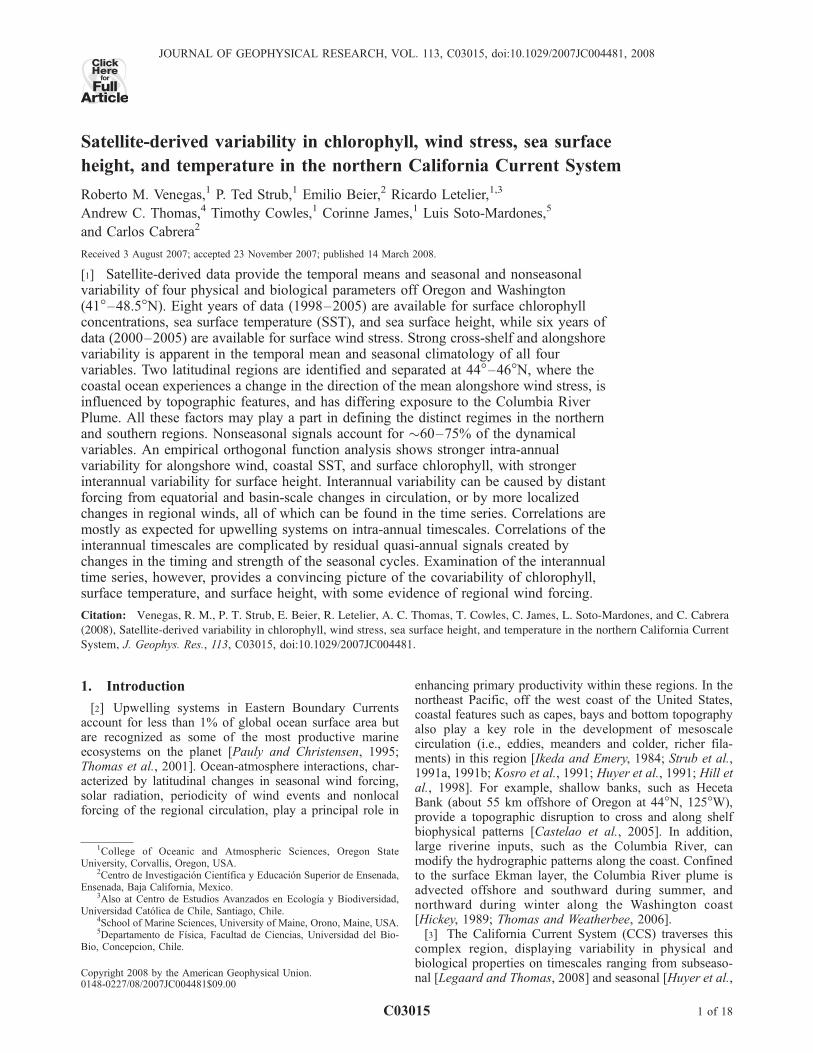
[8] The study region is shown in Figure 1, along with the200-m isobath (the approximate outer edge of the continen-tal shelf) and the identification of geographic featuresreferred to in the text. Over this region, we evaluate eightyears (January 1998 to December 2005) of satellite-derivedsurface CHL, SSH and SST data, and six years (January

Figure 1. Map of study region along the northernCalifornia Current System. The 200-m isobath is shown todenote the outer boundary of the shelf.

C03015 VENEGAS ET AL.: SATELLITE-DERIVED VARIABILITY IN THE NORTHERN CCS

2 of 18

C03015

2000 to December 2005) of TAU data. We examine theirtemporal means and seasonal cycles, then remove theseasonal cycles to analyze at the nonseasonal variability.The nonseasonal variability is, in turn, divided into decadal,interannual and intra-annual timescales.[9] Chlorophyll concentrations come from the Sea View-

ing Wide Field of View Sensor (SeaWiFS), using the OC4version 3 algorithm with standard NASA global coefficients[O’Reilly et al., 1998] at 1.2 km resolution. Daily fields arecomposited to form 8-day fields. SST data come from theAdvanced Very High-Resolution Radiometer (AVHRR) onthe NOAA-14 to NOAA-18 satellites. SST composites at1.1 km resolution were constructed by selecting the clearest(less than 50% cloud coverage) several images in each 8-dayperiod, then using the warmest value at each pixel. Thisdoes not eliminate all clouds but reduces their influence andavoids the large loss of data caused by presently available(very conservative) cloud masks. Sea surface wind stressdata come from daily QuikSCAT data in the Jet PropulsionLaboratory (JPL) archive. Averages are formed from dailyfields over the same 8-day periods used for SST and CHL,with quarter-degree resolution.[10] The along-track altimeter SSH data are also obtained

from the JPL archive and include data from TOPEX andJason-1 (both with a 10-day exact repeat period), GeosatFollow On (GFO) (with a 17.5-day exact repeat period), andERS (with a 35-day exact repeat period) altimeters. Thesewere initially processed using standard atmospheric correc-tions to produce along-track sea level anomalies. Duringthis processing, the temporal means are removed from eachalong-track point to eliminate the unknown marine geoid.Gridded SSH fields are produced from the along-track SSHanomalies for 16-day periods using all available altimeters.Each period contains approximately one-and-a-halfTOPEX/Jason exact repeat cycles, approximately one GFOcycle and one-half ERS cycle. Since the ERS ground trackshave a 17.5-day subcycle, they fill in a GFO-like pattern ineach 16-day period. Before combining data from differentaltimeters into 2-D fields, the spatial mean over the study areafor each altimeter is removed to reduce residual orbit errors.To replace the long-term temporal mean SSH, a climatolog-ical sea surface dynamic height field (SSDH) relative to 500m was formed from the long-term means of temperature andsalinity [Levitus et al., 1998] and added to each along-trackSSH anomaly. Two-dimensional gridded SSH fields areproduced using the method of successive correction [Struband James, 2000] to combine all data from each 16-dayperiod. As a side effect of the processing, removal of thespatial mean for each altimeter in each 16-day period alsoremoves much of the dominant domain-wide annual rise andfall of SSH, caused by the large-scale seasonal steric heightchanges due to seasonal heating and cooling. This processdoes not remove the gradients that correspond to the spatialand temporal changes in geostrophic currents.[11] The long-term (8-year and 6-year) temporal means of

CHL, SST and TAU were formed from the 8-day compo-sites. The climatological SSDH field serves as a very coarsesubstitute for the temporal mean for SSH field. The 8-daySST, CHL and TAU fields were then averaged to formindividual 16-day fields, coincident with the 16-day SSHfields. These 16-day fields were averaged to form climato-logical monthly and bimonthly seasonal cycles.

[12] To form nonseasonal time series, harmonic seasonalcycles were first calculated by fitting annual and semiannualharmonics to each parameter at each grid point, using the16-day time series:

S tð Þ ¼ S0 þ Sa* cos wt � 81ð Þ þ Ss* cos 2wt � 82ð Þ þ res S tð Þ� �

;

where S(t) is time series; S0 is long-term mean; Sa is annualamplitude; Ss is semiannual amplitude; res is residuals; w isannual radian frequency (2p/365.25 days); t is time; and 81and 82 are phase of annual and semiannual harmonics.These seasonal cycles were subtracted from the 16-day timeseries to form nonseasonal fields. Note that this procedureremoves only the stationary component of the seasonality.For this reason, changes in phase and strength of seasonalcycles during the record will contribute to nonseasonalanomalies [Legaard and Thomas, 2008]. Coherent nonsea-sonal variability within these large data sets was simplifiedusing empirical orthogonal function (EOF) analyses basedon singular value decomposition [Preisendorfer, 1988;Emery and Thomson, 1998]. For the vector wind stress,we used a joint EOF analysis of the u and v wind stresscomponents simultaneously.[13] We quantified variance in each of a series of time-

scale bands for each variable over the entire region. Usingthe 16-day time series, temporal variances of each variableat each grid point are calculated from the original timeseries, then they are spatially averaged over the studyregion. The stationary (harmonic) seasonal cycles are thenremoved at each grid point and the variances are recalcu-lated. This quantifies the percent of total variance repre-sented by the stationary seasonal cycles and nonseasonalsignals. The first two EOF modes of the nonseasonal timeseries are then calculated (the nonseasonal EOF’s describedabove). Considering these to represent 100% of the spatiallycoherent nonseasonal ‘‘signal,’’ a quadratic fit and 11-point(176-day) running mean are then sequentially removed fromeach EOF time series, recalculating the variance afterremoving each signal. We refer to the long-period (quadraticfit) variability as the ‘‘decadal’’ variability, recognizing thatthe records are not long enough to characterize the realperiodicity on over these timescales. The 11-point runningmean is considered to represent ‘‘interannual’’ variabilityand the residual is called the ‘‘intra-annual’’ variability.Since the span of this filter is approximately 1=2 year, thehalf-power period is �1 year. Thus the intra-annual timeseries include periods of approximately one month (owingto the 16-day time step) to one year. The ‘‘interannual’’ timeseries have periods of one year and longer, lacking only thestationary harmonic seasonal cycles.[14] The above procedure characterizes the average var-

iance for each of the timescales over the region as a whole.Legaard and Thomas [2006, 2008] take a complementaryapproach, characterizing the seasonal, interannual and intra-seasonal variability at each grid point for SST and CHL.

3. Results

3.1. Temporal Mean Fields

[15] In this section we present the basic characteristics ofthe overall temporal means for the four variables. These areexamined in greater detail later in the manuscript.

C03015 VENEGAS ET AL.: SATELLITE-DERIVED VARIABILITY IN THE NORTHERN CCS

3 of 18

C03015

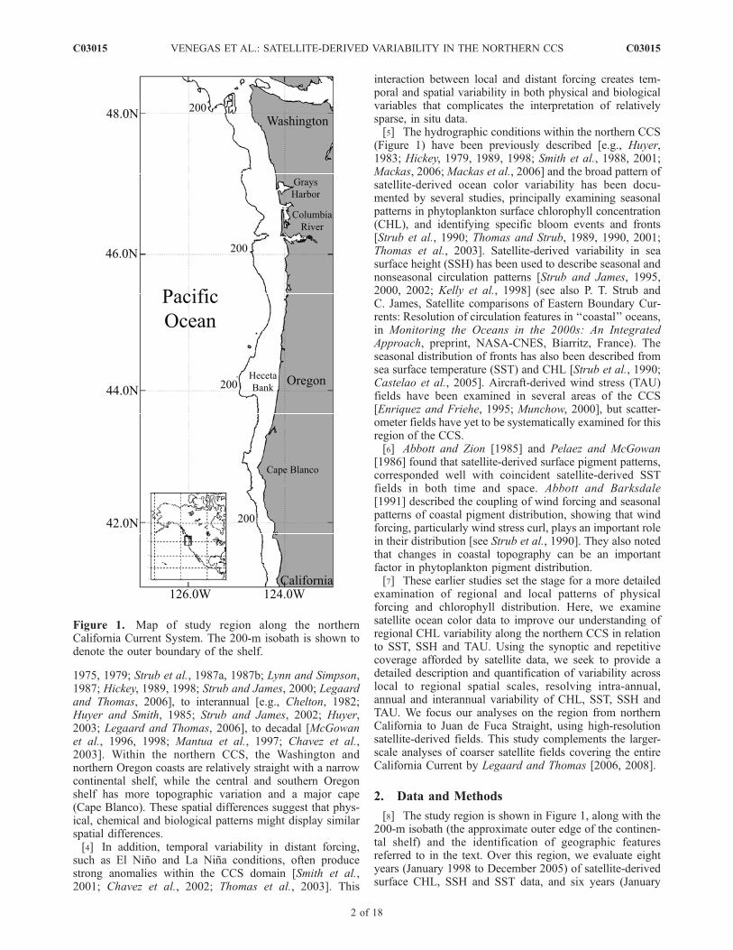
[16] The eight-year mean CHL distribution (Figure 2a)shows a strong onshore/offshore pattern, with a maximumconcentration near the coast, decreasing offshore (Figure 2a).The 200 m isobath generally lies just offshore of a coastalregion of concentrations higher than 5 mg m�3 north of�45�N, while south of �45�N the coastal concentrationsreach a maximum of 3.5 mg m�3. Offshore of the 200 misobath, an intermediate band of �150 km width contains

values between 0.3 and 2.5 mg m�3; farther offshoreconcentrations decrease to below 0.2 mg m�3. Theseregions approximately coincide with offshore zones de-scribed by others [e.g., Kahru and Mitchell, 2000; Legaardand Thomas, 2006; Henson and Thomas, 2007]. Highervalues over the shelf in the north may be partially due tomaterial other than chlorophyll originating from estuariesand the Columbia River.[17] Cold coastal and warm oceanic temperatures charac-

terize the SST temporal mean field (Figure 2b), consistentwith those described by Legaard and Thomas [2006] andothers. The coldest SST values occur close to the coastaround and southwest of Cape Blanco and north of GraysHarbor (47.0�N) over the shelf and in the Juan de FucaStraight (48.2�N, 124�W), while warm offshore wateroccurs south of �47�N (Figure 2b). SST shows the influ-ence of an equatorward summer jet along the 200-m isobatharound Heceta Bank, with colder water inshore of theisobath and jet.[18] As noted above, the mean SSDH relative to 500 m

(see Levitus et al. [1998] and Figure 2c) is calculated andadded to the SSH anomalies as a coarse proxy for thetemporal mean SSH field. In Figure 2c these data (on a 1�grid) have been mapped to the same grid as the othervariables. Although these data are highly smoothed, themean dynamic height field shows lower values around CapeBlanco and extending north along the Oregon Shelf, con-sistent with the wider regions of low SST in southern part ofthe domain (Figure 2b). The contribution of this SSH to thealtimeter fields is a general downward slope toward thecoast south of the Columbia River, consistent with anequatorward current, and a downward slope toward thenorthwest off the coast of Washington, depicting onshoreflow of the North Pacific Current off southern Washingtonand poleward flow off northern Washington.[19] The six-year TAU temporal mean (Figure 2d) shows

downwelling-favorable winds north of the Columbia River(�46.2�N) and upwelling-favorable winds south of 44.0�N.Between 44� and 46�N, the temporal mean of the wind ismostly onshore and upwelling-neutral, with a slightlynorthward component over the shelf.

3.2. Seasonal Climatology Fields

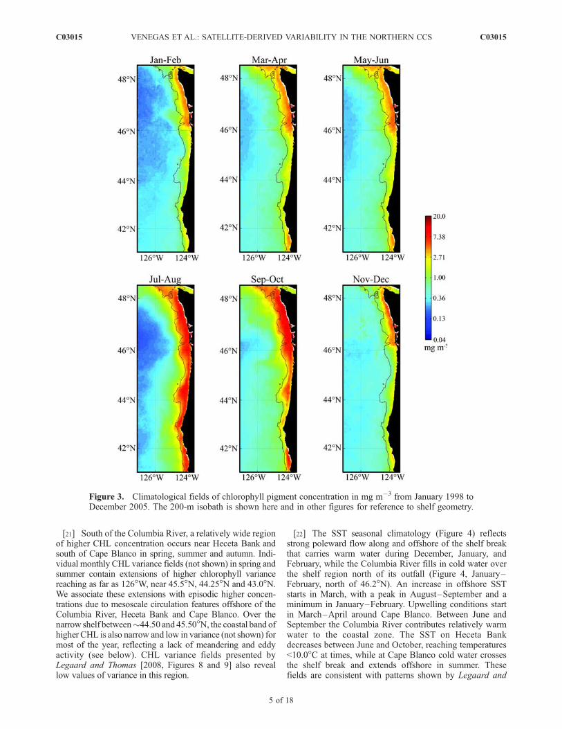
[20] The eight-year (1998–2005) bimonthly CHL sea-sonal climatology (Figure 3) depicts maximum concentra-tions inshore of the 200-m isobath in summer. These valuesdecrease in winter, especially south of the Columbia River(�46.2�N). North of the Columbia River, moderately highconcentrations continue to be seen in winter over the shelf.Individual monthly means for December and January (notshown) display the narrowest bands of elevated CHLconcentrations next to the coast, with the lowest valuesfound during the year (maxima less than 3 mg m�3). Thesevalues may reflect a contribution from CDOM and partic-ulate matter from the large estuaries and the Columbia RiverPlume, which flows northward in winter, trapped over theshelf by onshore Ekman transport [Hickey, 1998; Thomas etal., 2003]. Evidence for this is provided by Thomas andWeatherbee [2006], who show maps of normalized 555 nmwater leaving radiances, an indicator of particulate matter.Their winter patterns are very similar to the winter surfaceCHL distributions presented here.

Figure 2. Eight-year mean of (a) chlorophyll pigmentconcentration in mg m�3, (b) sea surface temperature in �C,(c) sea surface dynamic height derived as a long-term meandynamic topography in cm, with reference to 500 m andderived from Levitus et al. [1998] climatology, and (d) six-yearmean of QuikSCAT wind stress (TAU) in N m�2.

C03015 VENEGAS ET AL.: SATELLITE-DERIVED VARIABILITY IN THE NORTHERN CCS

4 of 18

C03015

[21] South of the Columbia River, a relatively wide regionof higher CHL concentration occurs near Heceta Bank andsouth of Cape Blanco in spring, summer and autumn. Indi-vidual monthly CHL variance fields (not shown) in spring andsummer contain extensions of higher chlorophyll variancereaching as far as 126�W, near 45.5�N, 44.25�N and 43.0�N.We associate these extensions with episodic higher concen-trations due to mesoscale circulation features offshore of theColumbia River, Heceta Bank and Cape Blanco. Over thenarrow shelf between�44.50 and 45.50�N, the coastal band ofhigher CHL is also narrow and low in variance (not shown) formost of the year, reflecting a lack of meandering and eddyactivity (see below). CHL variance fields presented byLegaard and Thomas [2008, Figures 8 and 9] also reveallow values of variance in this region.

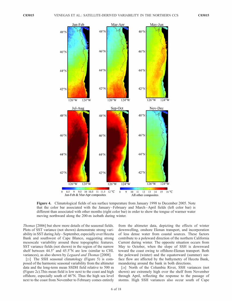
[22] The SST seasonal climatology (Figure 4) reflectsstrong poleward flow along and offshore of the shelf breakthat carries warm water during December, January, andFebruary, while the Columbia River fills in cold water overthe shelf region north of its outfall (Figure 4, January–February, north of 46.2�N). An increase in offshore SSTstarts in March, with a peak in August–September and aminimum in January–February. Upwelling conditions startin March–April around Cape Blanco. Between June andSeptember the Columbia River contributes relatively warmwater to the coastal zone. The SST on Heceta Bankdecreases between June and October, reaching temperatures<10.0�C at times, while at Cape Blanco cold water crossesthe shelf break and extends offshore in summer. Thesefields are consistent with patterns shown by Legaard and

Figure 3. Climatological fields of chlorophyll pigment concentration in mg m�3 from January 1998 toDecember 2005. The 200-m isobath is shown here and in other figures for reference to shelf geometry.

C03015 VENEGAS ET AL.: SATELLITE-DERIVED VARIABILITY IN THE NORTHERN CCS

5 of 18

C03015

Thomas [2006] but show more details of the seasonal fields.Plots of SST variance (not shown) demonstrate strong vari-ability in SST during July–September, especially overHecetaBank and southwest of Cape Blanco, suggesting strongmesoscale variability around these topographic features.SST variance fields (not shown) in the region of the narrowshelf between 44.5� and 45.5�N are low (similar to CHLvariances), as also shown by Legaard and Thomas [2008].[23] The SSH seasonal climatology (Figure 5) is com-

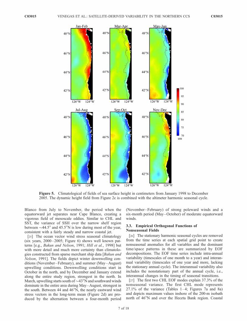
posed of the harmonic seasonal variability from the altimeterdata and the long-term mean SSDH field relative to 500 m(Figure 2c).This mean field is low next to the coast and highoffshore, especially south of 46�N. Thus the high sea levelnext to the coast from November to February comes entirely

from the altimeter data, depicting the effects of winterdownwelling, onshore Ekman transport, and incorporationof less dense water from coastal sources. These factorscontribute to a poleward direction of the northern CaliforniaCurrent during winter. The opposite situation occurs fromMay to October, when the slope of SSH is downwardtoward the coast owing to offshore-Ekman transport. Boththe poleward (winter) and the equatorward (summer) sur-face flow are affected by the bathymetry of Heceta Bank,meandering around the bank in both directions.[24] North of the Columbia River, SSH variances (not

shown) are extremely high over the shelf from Novemberthrough April, reflecting the response to the passage ofstorms. High SSH variances also occur south of Cape

Figure 4. Climatological fields of sea surface temperature from January 1998 to December 2005. Notethat the color bar associated with the January–February and March–April fields (left color bar) isdifferent than associated with other months (right color bar) in order to show the tongue of warmer watermoving northward along the 200-m isobath during winter.

C03015 VENEGAS ET AL.: SATELLITE-DERIVED VARIABILITY IN THE NORTHERN CCS

6 of 18

C03015

Blanco from July to November, the period when theequatorward jet separates near Cape Blanco, creating avigorous field of mesoscale eddies. Similar to CHL andSST, the variance of SSH over the narrow shelf regionbetween �44.5� and 45.5�N is low during most of the year,consistent with a fairly steady and narrow coastal jet.[25] The ocean vector wind stress seasonal climatology

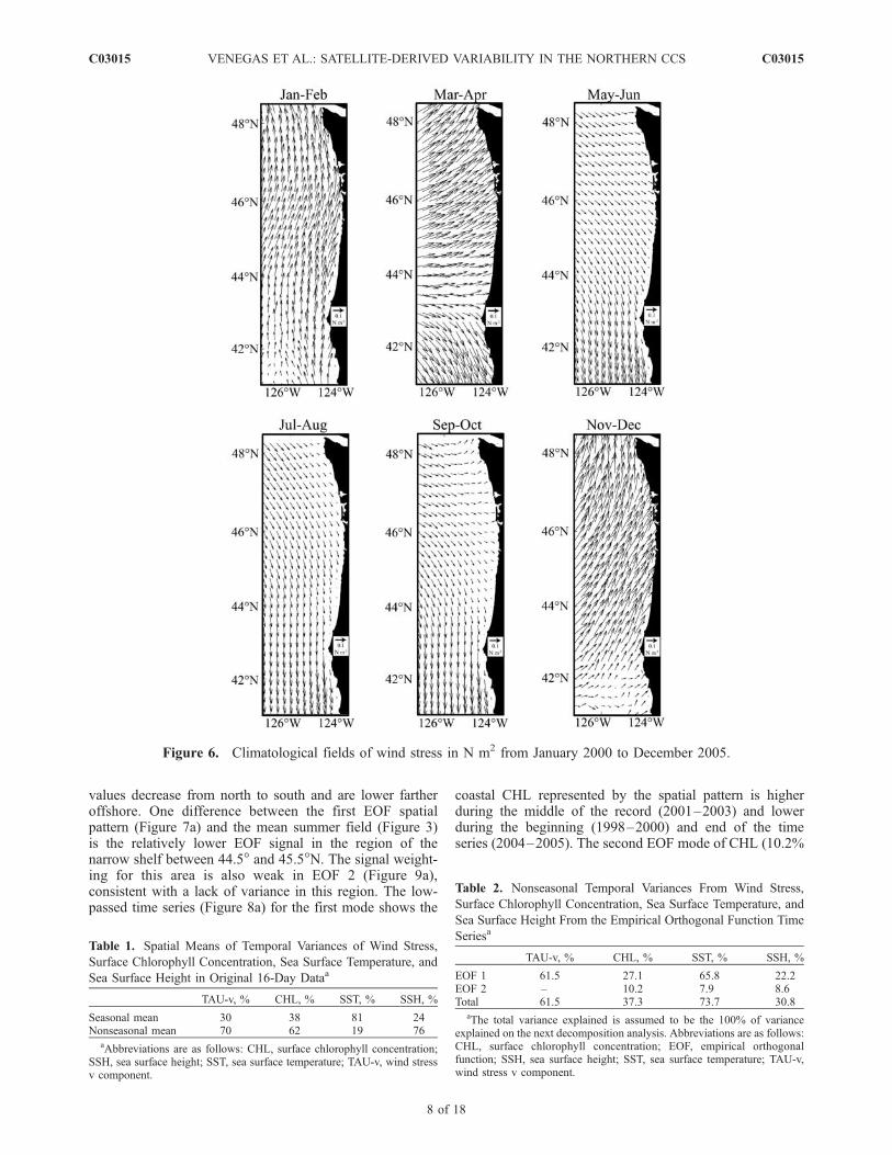
(six years, 2000–2005; Figure 6) shows well known pat-terns [e.g., Bakun and Nelson, 1991; Hill et al., 1998] butwith more detail and much more certainty than climatolo-gies constructed from sparse merchant ship data [Bakun andNelson, 1991]. The fields depict winter downwelling con-ditions (November–February), and summer (May–August)upwelling conditions. Downwelling conditions start inOctober in the north, and by December and January extendalong the entire study region, strongest in the north. InMarch, upwelling starts south of�43�Nand southwardwindsdominate in the entire area during May–August, strongest inthe south. Between 44 and 46�N, the nearly eastward windstress vectors in the long-term mean (Figure 2d) are pro-duced by the alternation between a four-month period

(November–February) of strong poleward winds and asix-month period (May–October) of moderate equatorwardwinds.

3.3. Empirical Orthogonal Functions ofNonseasonal Fields

[26] The stationary harmonic seasonal cycles are removedfrom the time series at each spatial grid point to createnonseasonal anomalies for all variables and the dominanttime/space patterns in these are summarized by EOFdecompositions. The EOF time series include intra-annualvariability (timescales of one month to a year) and interan-nual variability (timescales of one year and more, lackingthe stationary annual cycle). The interannual variability alsoincludes the nonstationary part of the annual cycle, i.e.,interannual changes in the timing of seasonal transitions.[27] The first two CHL EOF modes explain 37.3% of the

nonseasonal variance. The first CHL mode represents27.1% of the variance (Tables 1–4; Figures 7a and 8a)and depicts maximum values inshore of the 200-m isobathnorth of 46�N and over the Heceta Bank region. Coastal

Figure 5. Climatological of fields of sea surface height in centimeters from January 1998 to December2005. The dynamic height field from Figure 2c is combined with the altimeter harmonic seasonal cycle.

C03015 VENEGAS ET AL.: SATELLITE-DERIVED VARIABILITY IN THE NORTHERN CCS

7 of 18

C03015

values decrease from north to south and are lower fartheroffshore. One difference between the first EOF spatialpattern (Figure 7a) and the mean summer field (Figure 3)is the relatively lower EOF signal in the region of thenarrow shelf between 44.5� and 45.5�N. The signal weight-ing for this area is also weak in EOF 2 (Figure 9a),consistent with a lack of variance in this region. The low-passed time series (Figure 8a) for the first mode shows the

coastal CHL represented by the spatial pattern is higherduring the middle of the record (2001–2003) and lowerduring the beginning (1998–2000) and end of the timeseries (2004–2005). The second EOF mode of CHL (10.2%

Figure 6. Climatological fields of wind stress in N m2 from January 2000 to December 2005.

Table 1. Spatial Means of Temporal Variances of Wind Stress,

Surface Chlorophyll Concentration, Sea Surface Temperature, and

Sea Surface Height in Original 16-Day Dataa

TAU-v, % CHL, % SST, % SSH, %

Seasonal mean 30 38 81 24Nonseasonal mean 70 62 19 76

aAbbreviations are as follows: CHL, surface chlorophyll concentration;SSH, sea surface height; SST, sea surface temperature; TAU-v, wind stressv component.

Table 2. Nonseasonal Temporal Variances From Wind Stress,

Surface Chlorophyll Concentration, Sea Surface Temperature, and

Sea Surface Height From the Empirical Orthogonal Function Time

Seriesa

TAU-v, % CHL, % SST, % SSH, %

EOF 1 61.5 27.1 65.8 22.2EOF 2 – 10.2 7.9 8.6Total 61.5 37.3 73.7 30.8

aThe total variance explained is assumed to be the 100% of varianceexplained on the next decomposition analysis. Abbreviations are as follows:CHL, surface chlorophyll concentration; EOF, empirical orthogonalfunction; SSH, sea surface height; SST, sea surface temperature; TAU-v,wind stress v component.

C03015 VENEGAS ET AL.: SATELLITE-DERIVED VARIABILITY IN THE NORTHERN CCS

8 of 18

C03015

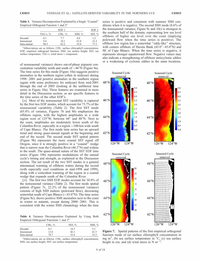
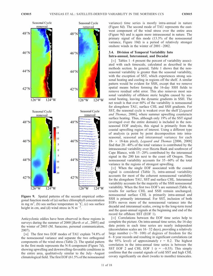
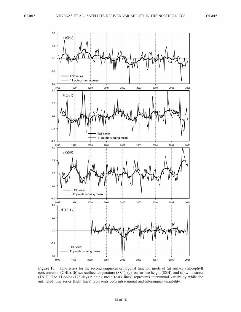
of nonseasonal variance) shows out-of-phase pigment con-centration variability north and south of �46�N (Figure 9a).The time series for this mode (Figure 10a) suggests positiveanomalies in the northern region (often in midyear) during1998–2001 and positive anomalies in the southern region(again with some preference for midyear) from mid-2001through the end of 2005 (looking at the unfiltered timeseries in Figure 10a). These features are examined in moredetail in the Discussion section, as are specific features inthe time series of the other EOF’s.[28] Most of the nonseasonal SST variability is captured

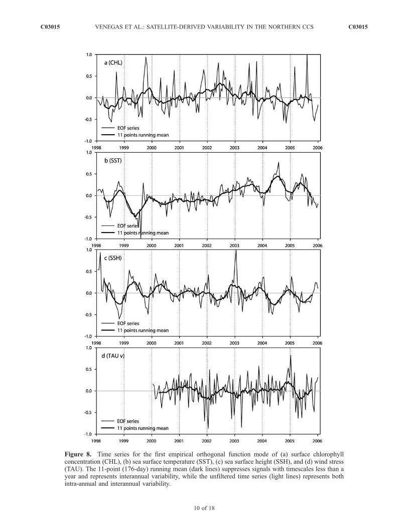
by the first two EOF modes, which account for 73.7% of thenonseasonal variability (Table 2). The first SST mode(65.8% of variance, Figures 7b and 8b) emphasizes theoffshore region, with the highest amplitudes in a wideregion west of 125�W, between 44� and 48�N. Next tothe coast, amplitudes are moderately lower south of theColumbia River, especially in a region �100-km wide southof Cape Blanco. The first mode time series has an upwardtrend and strong quasi-annual signals at the beginning andend of the record. The second mode SST spatial pattern(Figure 9b) represents the more coastal SST signal offOregon, since it is strongly positive in a ‘‘coastal’’ wedgethat is narrow near the Columbia River (46.2�N) and widensto the south. The quasi-annual nature of the SST EOF timeseries (Figure 10b) represents modulations of the annualcycle’s timing and strength, as explained in the Discussionsection. The net result of the two SST modes is a generalinterannual warming of offshore waters during the record(with especially cool conditions in mid-1998 and 1999),along with a coincident warming of the region in a coastalwedge that expands south of the Columbia River.[29] The first two SSH EOF modes account for 30.8% of

the nonseasonal variance (Table 2). The first mode spatialpattern (Figure 7c, 22.2% of the nonseasonal variance)consists of high SSH inshore (poleward flow), decreasingsomewhat south of Cape Blanco (�43.0�N). The time series(Figure 8c), shows positive SSH anomalies next to the coastin winter or autumn, except during 2000–2001. This isconsistent with the winter SSH climatology when the time

series is positive and consistent with summer SSH con-ditions when it is negative. The second SSH mode (8.6% ofthe nonseasonal variance, Figure 9c and 10c) is strongest inthe southern half of the domain, representing low sea leveloffshore of higher sea level over the coast (implyingpoleward flow when the time series is positive). Theoffshore low region has a somewhat ‘‘eddy-like’’ structure,with centers offshore of Heceta Bank (43.0�–45.0�N) andSE of Cape Blanco. When the time series is negative, itrepresents stronger equatorward flow. Negative values mayalso indicate a strengthening of offshore anticyclonic eddiesor a weakening of cyclonic eddies in the same locations.

Table 3. Variance Decomposition Explained by a Single ‘‘Coastal’’

Empirical Orthogonal Function 1 and 2a

EOF 1 EOF 2

TAU-v, % CHL, % SSH, % SST, %

Decadal 0.1 7.7 4.0 1.2Interannual 9.4 10.1 61.0 21.5Intra-annual 90.5 82.2 35.0 77.3

aAbbreviations are as follows: CHL, surface chlorophyll concentration;EOF, empirical orthogonal function; SSH, sea surface height; SST, seasurface temperature; TAU-v, wind stress v component.

Table 4. Variance Decomposition Explained by Using Both

Empirical Orthogonal Functions 1 and 2a

CHL, % SST, % SSH, %

Decadal 8.3 18.5 5.2Interannual 12.0 46.1 61.5Intra-annual 79.7 35.4 33.3

aAbbreviations are as follows: CHL, surface chlorophyll concentration;SSH, sea surface height; SST, sea surface temperature.

Figure 7. Spatial patterns of the first empirical orthogonalfunction mode of (a) surface chlorophyll concentration inmg m3, (b) sea surface temperature in �C, (c) sea surfaceheight in cm; and (d) wind stress in N m�2.

C03015 VENEGAS ET AL.: SATELLITE-DERIVED VARIABILITY IN THE NORTHERN CCS

9 of 18

C03015

Figure 8. Time series for the first empirical orthogonal function mode of (a) surface chlorophyllconcentration (CHL), (b) sea surface temperature (SST), (c) sea surface height (SSH), and (d) wind stress(TAU). The 11-point (176-day) running mean (dark lines) suppresses signals with timescales less than ayear and represents interannual variability, while the unfiltered time series (light lines) represents bothintra-annual and interannual variability.

C03015 VENEGAS ET AL.: SATELLITE-DERIVED VARIABILITY IN THE NORTHERN CCS

10 of 18

C03015

Anticyclonic eddies have been observed in these regions insurveys during the summer of 2000 [Barth et al., 2005] andthe winter of 2003 (M. Saraceno, personal communication,2007).[30] The first two EOF modes of TAU explain 74.8% of

the nonseasonal variance and separate the two orthogonalcomponents of the wind stress (Table 2). The spatial patternin the first mode represents the N-S component (Figure 7d),showing upwelling and downwelling-favorable conditions inthe entire area, qualitatively similar to the July–Augustclimatological field. The first EOF (61.5% of the nonseasonal

variance) time series is mostly intra-annual in nature(Figure 8d). The second mode of TAU represents the east-west component of the wind stress over the entire area(Figure 9d) and is again more intraseasonal in nature. Theprimary signal of this mode (13.3% of the nonseasonalvariance, Figure 10d) is a period of relatively strongeronshore winds in the winter of 2001–2002.

3.4. Division of Temporal Variability IntoIntra-annual, Interannual, and Decadal

[31] Tables 1–4 present the percent of variability associ-ated with each timescale, calculated as described in themethods section. In general, Table 1 shows that the non-seasonal variability is greater than the seasonal variability,with the exception of SST, which experiences strong sea-sonal heating and cooling in regions off the shelf. A similarpattern would be evident for SSH, except that we removespatial means before forming the 16-day SSH fields toremove residual orbit error. This also removes most sea-sonal variability of offshore steric heights caused by sea-sonal heating, leaving the dynamic gradients in SSH. Thenet result is that over 60% of the variability is nonseasonalfor alongshore TAU, surface CHL and SSH gradients. ForSST, the seasonal cycle is weakest over the shelf [Legaardand Thomas, 2006], where summer upwelling counteractssurface heating. Thus, although only 19% of the SST signal(averaged over the entire domain) is included in the non-seasonal EOF analysis, this signal is primarily from thecoastal upwelling region of interest. Using a different typeof analysis (a point by point decomposition into intra-seasonal, seasonal and interannual variance for each18- � 18-km pixel), Legaard and Thomas [2006, 2008]find that 20–40% of the total variance is contributed by theintraseasonal variability over Heceta Bank and southwest ofCape Blanco, with 15–20% contributed by the interannualsignal in the 200 km next to the coast off Oregon. Thusnonseasonal variability accounts for 35–60% of the totalvariance in the regions of strongest upwelling.[32] When the single EOF associated with the coastal

signal is considered (Table 3), intra-annual variabilityaccounts for most of the coherent nonseasonal variabilityfor the alongshore TAU, SST and surface CHL. Interannualvariability accounts for the majority of the SSH nonseasonalvariability. When the first two EOF’s are summed (Table 4),results for surface CHL and SSH remain unchanged;nonseasonal surface CHL is primarily intra-annual andSSH is primarily interannual. For SST, inclusion of bothEOFs moves more of the nonseasonal variance into thedecadal and interannual scales, owing to the long-term trendand the quasi-annual signals at the beginning and end of therecord for offshore SST (EOF 1).[33] Correlations between the EOF time series help to

complete the picture. On intra-annual time series, the 16-daydata points in each time series are nearly independent(decorrelation scales are 16–32 days), providing a relativelylarge number (�70–100) of degrees of freedom for the6–8 year records and resulting in significant correlations (atthe 95% level) of approximately r = 0.2. The highestcorrelation in the intra-annual time series is between theSST EOF 2 and CHL EOF 1 (r = �0.55). This simplyconfirms that the coastal signals of cold SST and high CHLcovary significantly on short (weeks to months) timescales.

Figure 9. Spatial patterns of the second empirical ortho-gonal function mode of (a) surface chlorophyll concentrationin mg m3, (b) sea surface temperature in �C, (c) sea surfaceheight in cm, and (d) wind stress in N m�2.

C03015 VENEGAS ET AL.: SATELLITE-DERIVED VARIABILITY IN THE NORTHERN CCS

11 of 18

C03015

Figure 10. Time series for the second empirical orthogonal function mode of (a) surface chlorophyllconcentration (CHL), (b) sea surface temperature (SST), (c) sea surface height (SSH), and (d) wind stress(TAU). The 11-point (176-day) running mean (dark lines) represents interannual variability while theunfiltered time series (light lines) represents both intra-annual and interannual variability.

C03015 VENEGAS ET AL.: SATELLITE-DERIVED VARIABILITY IN THE NORTHERN CCS

12 of 18

C03015

This variability is presumably driven by winds but we findmarginal correlations between the intra-annual time series ofsouthward alongshore TAU and the other variables at zerolag: CHL EOF 1 (r = +0.30), SST EOF 2 (r = �0.21) andSSH EOF 1 (r = �0.19). Correlations drop to near zero atlags of 1–2 time step (16–32 days). Although the signif-icance level and amount of variance explained are low, thesecorrelations are consistent with expected relationships inupwelling systems on timescales of weeks to months. Notethat the synoptic scale (3–10 days) is not resolved by the16-day composites/averages used in this study.[34] On interannual timescales, the time series are dom-

inated by residual quasi-annual signals discussed furtherbelow, which result in long decorrelation timescales and asmall number of degrees of freedom. Lagged correlationcoefficients are cyclical, making it difficult to assign statis-tical reliability. With this caveat, the highest correlationswith minimal lags are as follows: CHL EOF 1 and SST EOF2 (�0.56, lag of 16 days); CHL EOF 1 and SSH EOF 1(�0.52, lag of 16 days); SST EOF 2 and SSH EOF 1(+0.58, lag of 32 days); and CHL EOF 2 and SST EOF 2(�0.54, zero lag). No significant correlations betweenalongshore TAU and the other variables were present atlags of 0 to 48 days. There are higher correlations at longerlags between TAU EOF 1 and the other variables, but theymake little physical sense: CHL EOF 1 (�0.43, lag of twomonths); SST EOF 2 (+0.52, lag of 4 months); SSH 1(�0.21, lag of 5 months).

4. Discussion

4.1. Spatial Variability: Two Major Dynamical Regionsand Their Annual Cycles

[35] In general, the patterns of coastal CHL are consistentwith previous views of the large-scale chlorophyll patternsalong the northern California Current [Strub et al., 1990;Thomas and Strub, 1989, 1990, 2001; Thomas et al., 1994,2001, 2003; Legaard and Thomas, 2006], where high CHLvalues are evident north of 46�N, with seasonal maxima inspring and summer and minima in winter (Figure 3).Extending this to SSH, SST and alongshore TAU, we findspatial and temporal patterns that divide this domain intotwo dynamic northern and southern regions, separatedsomewhere between Cape Blanco and the mouth of theColumbia River (43–46�N), depending on the variableconsidered.[36] Considering surface forcing, upwelling-favorable

winds (Figure 6) begin first in spring south of Cape Blanco,spreading to the north in summer; downwelling-favorablewinds begin first in autumn north of the Columbia River,extending to the south in winter. The fields of SSH (Figure 5)next to the coast follow this forcing fairly directly, droppingfirst south of 45�N in March–April and rising first north of45�N in November–December. The largest region of lowSSH is around and south of Cape Blanco, where there areeight months of upwelling-favorable and four months ofdownwelling-favorable TAU. The offshore movement ofthe SSH gradient corresponds to the offshore movementand separation from the coast of the equatorward jet insummer [Barth et al., 2000; Strub and James, 2000].[37] One of the new and interesting aspects of the SSH

analysis is the degree to which it confirms the topographic

control of both poleward and equatorward flow around theHeceta Bank region. Previous studies have demonstratedthe topographic deflection of the equatorward summer jetby capes and subsurface topography [Haidvogel et al.,2001; Barth et al., 2005; Castelao et al., 2005]. Haidvogelet al. [1991] modeled this deflection around an idealizedcape for equatorward flow, but also found a deflection of themean flow around the cape for poleward flow. The meanaltimeter SSH fields in winter are consistent with this modelresult. The model also shows that the deflection of thepoleward flow in winter produces filaments and meanderswith an order of magnitude less EKE than the deflection ofthe equatorwad flow, consistent with the seasonal variationsin altimeter EKE (lower values in winter next to the coast)described by Kelly et al. [1998], Strub and James [2000]and quantified by Keister and Strub [2008].[38] Interpretation of the relation between SSH and SST

(Figure 4) fields is complicated by the presence of the coldColumbia River plume over the Washington shelf in winterand the coincidence of summer warming and upwelling.Thus lower SST values occur in the north over the shelf inwinter, coincident with higher SSH values caused bydownwelling, while lower SST values occur in the southover the shelf in summer, coincident with lower SSH valuesproduced by the denser, upwelled water. Offshore, we findthe expected pattern of relatively higher SST in late sum-mer, with lower values in late winter (Figure 4).[39] The Columbia River plume also complicates inter-

pretation of the CHL fields, due to CDOM (and suspendedsediments) over the Washington shelf. These contribute tothe appearance (Figure 3) of high CHL in winter [Thomasand Weatherbee, 2006]. How much of this is real chloro-phyll pigments remains to be determined, especially giventhe low values of chlorophyll pigment concentrations ob-served by in situ measurements over the Washington shelfin winter [Hermann et al., 1989]. The summer spatialpattern of CHL is probably more realistic, showing highvalues everywhere over the shelf, again revealing theinfluence of Heceta Bank and Cape Blanco in creatingregions of expanded high concentrations inshore and off-shore of the 200 m isobath (respectively), coincident withlower SST and SSH values. Maximum CHL values occur inAugust–September and reach more than 10 mg m�3 in thenorth. Similar CHL concentrations for the Washington shelfhave been reported previously by Hermann et al. [1989],with blooms in excess of 20 mg m�3 on the Washingtonmidshelf during the summer months.[40] South of the Columbia River, CHL shows expected,

consistent, inverse relationships with SST and SSH over theshelf: lower (higher) CHL values correspond to higher(lower) SST and SSH values in autumn-winter (spring-summer), as lower SSH fields over colder, denser andnutrient-rich water upwelled in spring-summer change tohigher SSH values over the warmer, less dense and nutrientpoor offshorewater that is transported next to the coast duringwinter downwelling. This inverse relationship between CHLand both SSH and SST is also reflected in the correlationcoefficients on both intra-annual and interannual timescales.[41] The point by point analysis of Legaard and Thomas

[2006] provides some context for the wedge-like pattern ofnonseasonal SST EOF 2 south of the Columbia River. Thispattern is similar to the northern end of the region with the

C03015 VENEGAS ET AL.: SATELLITE-DERIVED VARIABILITY IN THE NORTHERN CCS

13 of 18

C03015

lowest magnitude of the annual harmonic over the entireCalifornia Current, and a greater percent of variance in thenonseasonal signals. The larger pattern shown by Legaardand Thomas continues to expand as one moves south alongthe California coast. The region with the highest annualamplitude is found offshore of Oregon and Washington, asalso found here.[42] The division of the coastal region between 41� and

48.5�N into two dynamic regimes is similar to the divisionsuggested by Huyer et al. [2005]. Using repeated hydro-graphic transects off 44.6�N and 41.9�N, Huyer et al.[2005] describe Cape Blanco (42.9�N) as dividing the fieldsfrom the two latitudes during summer upwelling. They findstronger upwelling winds south of the cape, similar to thefields in Figure 6 (May–October). Likewise, they describean upwelling front and jet that is farther offshore south ofthe Cape, similar to the satellite SST and SSH fields for thesame months presented in Figures 4 and 5 and consistentwith climatological cross-shelf pigment patterns [Thomasand Strub, 2001]. The higher phytoplankton biomass theyfind in the south is represented in the satellite surfacechlorophyll fields in May–June, but is not apparent in theJuly–August fields. This may reflect a difference betweenintegrated biomass values from their in situ data, comparedto the surface pigment fields from satellite data presentedhere. The satellite fields, however, make it clear that there isconsiderable alongshore variability in the width of thehigher surface pigment fields, especially north of CapeBlanco. On a larger scale, Legaard and Thomas [2008]identify Cape Mendocino (40�–41�N) as the dividing pointfor regions in the entire California Current. Thus, on anyscale examined, statistical analyses will divide the Califor-nia Current into a few latitudinal subdomains. This is usefulas a first-order characterization, but it will always oversim-plify and ignore the large degree of alongshore and cross-shore variability on smaller and larger scales.[43] A final note concerning spatial variability draws

attention to the region of narrow shelf and low variabilitybetween 44.5� and 45.5�N. Seasonal monthly mean fields ofCHL, SST and SSH are typically narrower in this region, asare the spatial fields for the nonseasonal EOF’s. Likewise,monthly mean variance fields (not shown) for CHL, SSTand SSH have distinct minima in this region. This is theregion chosen for observation by the Coastal UpwellingExperiments (CUE) in the early 1970’s, which resulted infairly simple (and useful) first-order descriptions of 2-D(onshore-offshore) coastal upwelling [Huyer et al., 1978].The location was chosen by examining the bottom topog-raphy and selecting the region with the simplest localvariability, after initial surveys farther south, which proveddifficult to interpret (A. Huyer, personal communication,2007). We can see now that the location selected for CUEwas the best choice for steady seasonal (summer) conditionsand a lack of temporal variability. Choice of regions 100 kmto the north or south would have resulted in a much morecomplicated initial picture of coastal upwelling.

4.2. Interannual Temporal Variability: El NinoSouthern Oscillation, Other Distant Forcing, andChanges in Seasonal Timing

[44] On the shorter, intra-annual (monthly and to annual)timescales, we find the expected covariabilities between

TAU, CHL, SST and SSH. SST and CHL are negativelycorrelated, as described by Abbott and Zion [1985]. Equa-torward alongshore wind stress is (moderately or marginal-ly) correlated with higher CHL, lower SST and lower SSH.We concentrate below on the interannual timescales.[45] Some of the interannual variability represents the

midlatitude expression of the equatorial El Nino SouthernOscillation (ENSO) cycle [Huyer and Smith, 1985; Struband James, 2002]. During the period studied here, therewere strong and moderate El Nino events in 1997–1998and 2002–2003, respectively. Our time series only margin-ally catch the end of the strong event. A strong La Ninaoccurred from late 1998 at least until early 2000 (or into2001, depending on the variable examined). However, thereare also factors other than the ENSO cycle that createinterannual variability in the northern California Current.[46] In Figure 11, we have overlaid some of the interan-

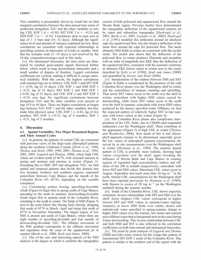
nual time series, after removing the quadratic fit, which wewill refer to as the trend. Unfortunately, the 11-point filterused to define the interannual timescale also eliminates theend of the 1997–1998 El Nino. This is seen by comparingthe first EOF of SSH (Figure 11a, dark line) with theMultivariate ENSO Index (MEI; Figure 11d). The MEIdrops from high values to 0 by mid-1998, when the SSHEOF 1 time series begins (the SSH EOF 1 time series showsthe final fall to zero in mid-1998). However, the unfilteredSSH EOF 1 time series in Figure 8c clearly shows the dropin SSH during the end of the El Nino in the first half of1998. The unfiltered SSH EOF 1 also shows a spike in early2003, while the filtered SSH-1 in Figure 11 is high inautumn and winter, 2002–2003, during the moderate event.There do not appear to be strong signatures of the 2002–2003 event in the interannual time series for coastal SST,CHL or alongshore TAU. The cold SST values associatedwith the La Nina (1999–2001) are seen primarily in thetime series for SST EOF 1 (Figures 8b and 11b), whichrepresents the more offshore SST signal (note that inFigures 8 and 10, trends are not removed; in Figure 11, they are).[47] The MEI and NINO4 time series in Figure 11d have

not been detrended and show a shift from cooler La Ninaconditions in 1999 to warmer, more El Nino-like conditionsduring 2002 + 2005. Comparisons to (un-detrended) timeseries for SST EOF 1 (Figure 8) and CHL EOF 2 (Figure10) show trends that indicate warming of the offshorewaters (SST EOF 1) and a shift from higher CHL in thenorth to higher CHL in the south (CHL EOF 2). However,correlations between the MEI and NINO4 indices and theinterannual time series shown in Figure 11 are not enhancedby the trends, since the EOF time series have beendetrended. The correlations between SST EOF 2 and theMEI and NINO4 are +0.32 and +0.39, respectively, withhighest correlations at zero lag. The correlations betweenSSH EOF 1 and the MEI and NINO4 are +0.35 and +0.37with lags of 16 and 48 days, respectively. These are lowerthan the approximate 0.50 values needed for significance atthe 95% level (for 15 df), although they are of the right signfor expected teleconnections between the equator and thePacific Northwest.[48] In the northern part of the California Current, there

are interannual changes in conditions that are not due toENSO changes. One is a well documented equatorward andonshore intrusion of colder and nutrient-rich subarctic water

C03015 VENEGAS ET AL.: SATELLITE-DERIVED VARIABILITY IN THE NORTHERN CCS

14 of 18

C03015

within the pycnocline during 2002 [Freeland et al., 2003;Huyer, 2003; Wheeler et al., 2003; Thomas et al., 2003;Strub and James, 2003]. The interannual SST EOF 2 timeseries in Figure 11a and 11d shows the coldest summer SSTvalues in mid-2002, excepting the late drop in SST in 2005.

These are due to strong summer spikes of negative SSTvalues in mid-2002 in the unfiltered SST EOF 2 time series(Figure 10), also present in mid-2003. The interannual CHLEOF 1 time series in Figures 8 and 11 shows generally highvalues through most of 2002 that were produced by a

Figure 11. Overlays of the interannual (176-day running mean filter) time series for a number of theempirical orthogonal functions (EOFs). (a) Coastal sea surface height (SSH) EOF 1 (dark line), coastalsea surface temperature (SST) EOF 2 (light line), and alongshore wind stress (TAU) EOF 1 (dashed line);(b) coastal SSH EOF 1 (dark line) and offshore SST EOF 1 (light line); (c) coastal surface chlorophyllconcentration (CHL) EOF 1 (dark line) and coastal SSH EOF 1 (light line); (d) coastal CHL EOF 1 (darkline) and coastal SST EOF 2 (light line); and (e) Multivariate ENSO Index (MEI) (dotted line) andNINO4 SST (solid line) El Nino indices.

C03015 VENEGAS ET AL.: SATELLITE-DERIVED VARIABILITY IN THE NORTHERN CCS

15 of 18

C03015

number of unfiltered (Figure 8) positive peaks, with fewnegative values. A period of negative values for the timeseries of SSH EOF 1 in Figure 11a during the first half of2002 has been interpreted to indicate stronger equatorwardflow of the subarctic water [Strub and James, 2003], priorto lower SST and higher CHL values.[49] Another period of unusual conditions off Oregon and

Washington was the ‘‘warm anomaly’’ of spring 2005[Hickey et al., 2006]. This event is attributed to weak andintermittent upwelling-favorable winds during spring andearly summer off Oregon and northern California [Hickey etal., 2006; Barth et al., 2007]. The time series for the EOF ofalongshore (equatorward) TAU (Figures 8d and Figure 11a)shows strong equatorward wind anomalies in autumn-winter 2004 (indicating weaker downwelling than usual),followed by strong poleward wind anomalies in spring-summer 2005 (indicating weaker upwelling). The interan-nual time series for SST EOF 1 (offshore SST, Figure 8) andSST EOF 2 (coastal SST, Figure 10) both show warmanomalies extending from mid-2004 through mid-2005.The unfiltered coastal CHL values (CHL EOF 1, Figure 8)depict lower CHL values in fall 2004 and spring 2005. Twospikes of CHL in the unfiltered 2005 data follow brief periodsof upwelling-favorable winds in late January–February andJuly 2005 [see also Henson and Thomas, 2007]. The timeseries are consistent with weak regional wind forcing inautumn-winter (weak downwelling), followed by late andweak upwelling during spring and the first half of summer,during this (approximately) one-year event.[50] Perhaps the most notable feature of the interannual

time series is the presence of quasi-annual cycles, even afterremoving the stationary harmonic seasonal cycles. Thisaffects the calculations of the correlations between theinterannual time series, producing correlation coefficientsthat cycle from high-to-low-to-high with a period of approx-imately one year. In our discussions of correlations betweenthe interannual time series, we only used peaks in correlationwith lags of zero to two 16-day time periods (one month lag,maximum). The primary purpose for Figure 11 is to showthese time series overlaid, in order to allow a clear picture andevaluation of the relationships that create those correlations.[51] Figure 11 shows two periods during which the quasi-

annual cycles are fairly well related, 1998–2000 and 2002–2005, separated by a period when these relationships breakdown (late 2000 through 2001). Perhaps more importantly,the timing of the quasi-annual signals changes after 2001.For example, SSH EOF 1 and SST EOF 2 are positivelycorrelated (r = +0.55), with peaks in the first half of the yearprior to 2001 and peaks in the second half of the year after2001. The cycles are not as clear for SST EOF 1 (Figure11b) and CHL EOF 1 (Figure 11c), but they change frompeaks occurring approximately late in the year in the earlyrecord to midyear at the end of the record. CHL EOF 1 alsocovaries out of phase with SSH EOF 1 (Figure 11c) andSST EOF 2 (Figure 11d). These represent changes in thetiming of the seasonal cycles, which cannot be fit by thephase-locked harmonic seasonal cycles, producing the qua-si-annual cycles in the interannual variability. Thus thecorrelations of the interannual time series do not representonly interannual variability with timescales of 2–7 years,but also include interannual variability in the timing andstrength of the annual seasonal cycles.

[52] Although the quasi-annual nature of the signals makesinterpretations of cyclical correlations problematic, the timeseries in Figure 11 demonstrate a high degree of covariabilityon scales shorter than quasi-annual. Examples include CHLEOF 1 and SST EOF 2 (Figure 11d; late 1998 and early 1999and 2003) and CHL EOF 1 and SSH EOF 1 (Figure 11c; late2002 to 2003). Even TAU EOF 1, although not significantlycorrelated over the entire record, shows covariability withSST EOF 2 (Figure 11a; 2000–2003). The wind stress timeseries is short and the relation appears to break down inwinter 2004–2005, yet 2005 is the best documented case inwhich regional winds were clearly responsible for a delayin the upwelling season, the 2005 warm event [Hickey et al.,2006;Kosro et al., 2006; Barth et al., 2007]. Thus winds playan important role. Although attributing the change in sea-sonal cycle timing to a single cause with statistical certainty isnot possible with the present, short data set, the time series inFigure 11 provide examples demonstrating that interannualchanges in the circulation, SST and CHL can be driven bycombinations of distant forcing from ENSO (1997–1998),effects of non-ENSO basin-scale circulation [2002] andregional winds (2005). Even using longer data sets (notsatellite), with other years showing delayed or weak upwell-ing (similar to 2005), Schwing et al. [2006] find it difficult toattribute the cause to a single large-scale climate index. Theyconclude that the CCS upwelling system is too complex todescribe with one such index.[53] We note, however, that identifying changes in the

timing of the seasonal cycles is an important result in itself.Variability in the timing of the circulation (SSH) and waterproperties (SST and CHL) have important ecological con-sequences, creating mismatches between different parts ofthe food chain (phytoplankton productivity, emergence ofresting stages of zooplankton, migrations of juvenile fish,seabird breeding and feeding of young, etc.), as discussedby Cushing [1990], Barth et al. [2007], Sydeman et al.[2006] and Brodeur et al. [2006]. These types of changesare also hypothesized as possible consequences of climatechange [Snyder et al., 2003]. Further analyses of presentdata sets which examine the mechanisms in detail may helpto improve our understanding of how climate change mayaffect ecosystems in the northern California Current, alongwith our ability to model those effects.

5. Conclusions

[54] Using 8 years of satellite-derived CHL, SSH, SSTdata and 6 years of TAU data over the northern CaliforniaCurrent, we draw the following conclusions:[55] 1. The mean fields and seasonal cycles of circulation

(SSH) and water properties (SSH, SST) are mostly asexpected, with an emphasis on the importance of topo-graphic forcing by the Heceta Bank and Cape Blanco duringboth winter and summer (Figures 3–6).[56] 2. The latitude band where the mean wind stress

switches from upwelling to downwelling-favorable is be-tween 44� and 46� N (Figure 2). Mean alongshore windstress is approximately upwelling-neutral in this band,owing to the cancellation of seasonally alternating windsof equal strength (Figure 6).[57] 3. The region from northern California to the Cana-

dian border separates into two general areas, with a dividing

C03015 VENEGAS ET AL.: SATELLITE-DERIVED VARIABILITY IN THE NORTHERN CCS

16 of 18

C03015

region around 44�–46� N. This may be due to wind forcing,topography or the presence of the Columbia River Plume(Figures 7 and 9). However, detailed fields show a greatdeal of alongshore and cross-shelf variability, including aregion of low variability over the narrow shelf between44.5� and 45.5� N (the classic 2-D upwelling system).[58] 4. In general, variability is dominated by nonseasonal

variability (60–75%) compared to seasonal variability (Ta-ble 1). The exception is SST, but that is controlled byoffshore seasonal warming, rather than dynamical signals.[59] 5. Nonseasonal variability in the coastal fields is

dominated by intra-annual variability (75–90%), comparedto interannual variability (Table 3; Figures 8 and 10). Theexception is coastal SSH (EOF1), where interannual vari-ability accounts for 60% of the nonseasonal variability.[60] 6. On intra-annual scales, the correlations are as

expected, with highest correlations between coastal CHLand SST, weaker correlations between alongshore TAU andthe other variables.[61] 7. On interannual timescales, the period of study

includes moderate ENSO variability, but is not dominatedby it. There are several non-ENSO interannual events,forced by changes in large-scale circulation (the 2002subarctic intrusion) and by local-regional changes in windforcing (the 2005 warm anomaly).[62] 8. Statistically, on interannual timescales, alongshore

TAU is not correlated significantly with the other variables.However, the TAU record is short and includes the apparentinfluence of the alongshore TAU on the 2005 warm anom-aly, as well as covariability with interannual fluctuations inSST during most of the record. All of the other variables arecorrelated at about jrj = 0.5–0.6.[63] 9. However, the correlations between coastal SSH,

SST and CHL on interannual timescales are difficult toevaluate owing to a residual quasi-annual signal in each record(Figure 11), caused by a change in the timing of the seasonalcycles. Visually, the time series appear correlated on severaltimescales, not just quasi-annual, providing evidence that thecovariability is real, although the forcing is still uncertain.[64] 10. The changes in timing of the seasonal cycles

need further study.

[65] Acknowledgments. Support for R. V. and P. T. S. was providedby the U.S. GLOBEC program in the northeast Pacific (National ScienceFoundation (NSF) grant OCE-0000900). Additional support for P. T. S. andR. L. was provided by the U.S. GLOBEC program (NOAA grantNA03NES00001), with partial support for P. T. S. also provided by NASAJet Propulsion Laboratory (JPL) (grant JPL-1206714-OSTM). Participationby E. B. is part of Consejo Nacional de Ciencia y Tecnologia (CONACYT)project SEP-2003-C02-42941/A-1. A. C. T. was supported by NSF grantsOCE-0535386 and OCE-0531289. Support for T. C. came from the NSF(U.S. GLOBEC program grant OCE-0001035). Altimeter data were pro-vided by JPL (http://podaac.jpl.nasa.gov/ost/). Scatterometer data wereprovided by Mike Freilich at Oregon State University and the JPL archive(http://winds.jpl.nasa.gov/). Sea surface temperature and Sea Viewing WideField of View Sensor (SeaWiFS) data were provided by the U.S. GLOBECprogram North East Pacific (NEP) project (http://coho.coas.oregonstate.edu/), the West Coast CoastWatch node (http://coastwatch.pfel.noaa.gov/)and the NASA Goddard Space Flight Center archive (http://oceancolor.gsfc.nasa.gov/). The manuscript benefited from the comments of two anonymousreviewers. This is contribution 561 of the U.S. GLOBEC program, jointlyfunded NSF and NOAA.

ReferencesAbbott, M. R., and B. Barksdale (1991), Phytoplankton pigment patternsand wind forcing off central California, J. Geophys. Res., 96, 14,649–14,667.

Abbott, M. R., and P. M. Zion (1985), Satellite observation of phytoplank-ton variability during an upwelling event, Cont. Shelf Res., 4, 661–680.

Bakun, A., and C. S. Nelson (1991), The seasonal cycle of wind stress curlin subtropical eastern boundary current regions, J. Phys. Oceanogr., 21,1815–1834.

Barth, J. A., S. D. Pierce, and R. L. Smith (2000), A separating upwellingcoastal jet at Cape Blanco, Oregon, and its connection to the CaliforniaCurrent System, Deep Sea Res., Part II, 47, 783–810.

Barth, J. A., S. D. Pierce, and R. J. Cowles (2005), Mesoscale structure andits seasonal evolution in the northern California Current System, DeepSea Res., Part II, 52, 5–28.

Barth, J. A., B. A.Menge, J. Lubchenco, F. Chan, J.M. Bane, A. R. Kirincich,M. A. McManus, J. Nielsen, S. D. Pierce, and L. Washburn (2007), De-layed upwelling alters nearshore coastal ocean ecosystems in the northernCalifornia current, Proc. Natl. Acad. Sci. U. S. A., 104, 3719–3724.

Brodeur, R. D., S. Ralston, R. L. Emmett, M. Trudel, T. D. Auth, and A. J.Phillips (2006), Anomalous pelagic nekton abundance, distribution, andapparent recruitment in the northern California Current in 2004 and 2005,Geophys. Res. Lett., 33, L22S08, doi:10.1029/2006GL026614.

Castelao, R. M., J. A. Barth, and T. P. Mavor (2005), Flow-topographyinteractions in the northern California Current System observed from geos-tationary satellite data, Geophys. Res. Lett., 32, L24612, doi:10.1029/2005GL024401.

Chavez, F. P., J. T. Pennington, C. G. Castro, J. P. Ryan, R. P. Michisaki,B. Schlining, P. Walz, K. R. Buck, A. McFayden, and C. A. Collins(2002), Biological and chemical consequences of the 1997–1998 ElNino in central California waters, Prog. Oceanogr., 54, 205–232.

Chavez, F. P., J. Ryan, S. E. Lluch-Cota, and M. Niguen (2003), Fromanchovies to sardine and back: Multidecadal changes in the PacificOcean, Science, 299, 217–221.

Chelton, D. B. (1982), Large-scale response of the California Current toforcing by wind stress curl, Rep. 23, pp. 130–148, Calif. Coop. OceanicFish. Invest., Univ. of Calif., San Diego, La Jolla, Calif.

Cushing, D. H. (1990), Plankton production and year-class strength in fishpopulations: An update on the match/mismatch hypothesis, Adv. Mar.Biol., 26, 249–293.

Emery, W. J., and R. E. Thomson (1998), Data and their analysis methodsin physical oceanography, 1st and 2nd eds., 634 pp., Pergamon Press,Amsterdam.

Enriquez, A. G., and C. A. Friehe (1995), Effects of wind stress andwind stresscurl variability on coastal upwelling, J. Phys. Oceanogr., 25, 1651–1671.

Freeland, H. J., G. Gatien, A. Huyer, and R. L. Smith (2003), Cold halo-cline in the northern California Current: An invasion of subarctic water,Geophys. Res. Lett., 30(3), 1141, doi:10.1029/2002GL016663.

Haidvogel, D. B., J. Wilkin, and R. Young (1991), A semi-spectral primi-tive equation ocean circulation model using vertical sigma and horizontalorthogonal curvilinear coordinates, J. Comp. Phys., 94, 151–185.

Haidvogel, D. B., A. Beckmann, and K. S. Hedstrom (2001), Dynamicalsimulations of filament formation and evolution in the Coastal TransitionZone, J. Geophys. Res., 96, 15,017–15,040.

Henson, S. A., and A. C. Thomas (2007), Interannual variability in timingof bloom initiation in the California Current System, J. Geophys. Res.,112, C08007, doi:10.1029/2006JC003960.

Hermann, A. J., B. M. Hickey, M. R. Landry, and D. F. Winter (1989),Coastal upwelling dynamics, in Coastal Oceanography of Washingtonand Oregon, edited by M. R. Landry and B. M. Hickey, pp. 211–254,Elsevier, New York.

Hickey, B. M. (1979), The California Current System-Hypotheses and facts,Prog. Oceanogr., 8, 191–279.

Hickey, B. M. (1989), Pattern and processes of circulation over the con-tinental shelf of Washington, in Coastal Oceanography of Washingtonand Oregon, edited by M. R. Landry and B. M. Hickey, pp. 41–115,Elsevier, New York.

Hickey, B. M. (1998), Coastal oceanography of western North Americafrom the tip of Baja California to Vancouver Island, in The Sea, vol.11, edited by A. R. Robinson and K. H. Brink, pp. 345–393, HarvardUniv. Press, Cambridge, Mass.

Hickey, B., A. MacFadyen,W. Cochlan, R. Kudela, K. Bruland, and C. Trick(2006), Evolution of chemical, biological, and physical water propertiesin the northern California Current in 2005: Remote or local wind for-cing?, Geophys. Res. Lett., 33, L22S02, doi:10.1029/2006GL026782.

Hill, A. E., B. M. Hickey, F. A. Shillington, P. T. Strub, K. H. Brink, E. D.Barton, and A. C. Thomas (1998), Eastern ocean boundaries, in The Sea,vol. 11, edited by A. R. Robinson and K. H. Brink, pp. 29–67, HarvardUniv. Press, Cambridge, Mass.

Huyer, A. (1983), Coastal upwelling in the California Current System,Prog. Oceanogr., 12, 259–284.

Huyer, A. (2003), Preface to special section on enhanced Subarctic influ-ence in the California Current, 2002, Geophys. Res. Lett., 30(15), 8019,doi:10.1029/2003GL017724.

C03015 VENEGAS ET AL.: SATELLITE-DERIVED VARIABILITY IN THE NORTHERN CCS

17 of 18

C03015

Huyer, A., and R. L. Smith (1985), The signature of El Nino of Oregon,1982–1983, J. Geophys. Res., 90, 7133–7142.

Huyer, A., R. D. Pillsbury, and R. M. Smith (1975), Seasonal variation ofalongshore velocity field over the continental shelf off Oregon, Limnol.Oceanogr., 20, 90–95.

Huyer, A., R. L. Smith, and E. J. C. Sobey (1978), Seasonal differences inlow-frequency current fluctuations over the Oregon continental shelf,J. Geophys. Res., 83, 5077–5089.

Huyer, A., E. J. Sobey, and R. L. Smith (1979), The spring transition in currentsover the Oregon continental shelf, J. Geophys. Res., 84, 6995–7011.

Huyer, A., P. M. Kosro, J. Fleischbein, S. R. Ramp, T. Stanton, L. Washburn,F. P. Chavez, T. J. Cowles, S. D. Pierce, and R. L. Smith (1991), Currentsand water masses of the Coastal Transition Zone off northern California,June to August 1988, J. Geophys. Res., 96, 14,809–14,832.

Huyer, A., J. H. Fleischbein, J. Keister, P. M. Kosro, N. Perlin, R. L. Smith,and P. A. Wheeler (2005), Two coastal upwelling domains in the northernCalifornia Current system, J. Mar. Res., 63, 901–929.

Ikeda, M., and W. J. Emery (1984), Satellite observations in modeling ofmeanders in the California Current System of Oregon and northernCalifornia, J. Phys. Oceanogr., 14, 1434–1450.

Kahru, M., and G. Mitchell (2000), Influence of 1997–1998 El Nino on thesurface chlorophyll in the California Current, Geophys. Res. Lett., 27,2937–2940.

Keister, J. E., and P. T. Strub (2008), Spatial and interannual variability inmesoscale circulation in the northern California Current System, J. Geo-phys. Res., doi:10.1029/2007JC004256, in press.

Kelly, K. A., R. C. Beardsley, R. Limeburner, K. H. Brink, J. D. Paduan,and T. K. Chereskin (1998), Variability of the near-surface eddy kineticenergy in the California Current based on altimeter, drifter, and mooredcurrent data, J. Geophys. Res., 103, 13,067–13,083.

Kosro, P. M., et al. (1991), The structure of the transition zone betweencoastal waters and the open ocean off northern California, winter andspring 1987, J. Geophys. Res., 96, 14,707–14,730.

Kosro, P. M., W. T. Peterson, B. M. Hickey, R. K. Shearman, and S. D.Pierce (2006), Physical versus biological spring transition: 2005,Geophys.Res. Lett., 33, L22S03, doi:10.1029/2006GL027072.

Legaard, K. R., and A. C. Thomas (2006), Spatial patterns in seasonaland interannual variability of chlorophyll and sea surface temperaturein the California Current, J. Geophys. Res., 111, C06032, doi:10.1029/2005JC003282.

Legaard, K. R., and A. C. Thomas (2008), Spatial patterns of intraseasonalvariability of chlorophyll and sea surface temperature in the CaliforniaCurrent, J. Geophys. Res., 112, C09006, doi:10.1029/2007JC004097.

Levitus, S., T. P. Boyer, M. E. Conkright, T. O’Brien, J. Antonov,C. Stephens, L. Stathopolos, D. Johnson, and R. Gelfeld (1998), WorldOcean Database 998, vol. 1, Introduction, NOAA Atlas NESDIS 18, Natl.Oceanic and Atmos. Admin., Silver Spring, Md.

Lynn, R. J., and J. J. Simpson (1987), The California Current System: Theseasonal variability of physical characteristics, J. Geophys. Res., 92,12,947–12,966.

Mackas, D. L. (2006), Interdisciplinary oceanography of the western NorthAmerican continental margin: Vancouver Island to the tip of Baja Cali-fornia, in The Sea, vol. 14, edited by A. R. Robinson and K. H. Brink, pp.441–502, Harvard Univ. Press, Cambridge, Mass.

Mackas, D. L., P. T. Strub, A. C. Thomas, and V. Montecino (2006), East-ern ocean boundaries, in The Sea, vol. 14, edited by A. R. Robinson andK. H. Brink, pp. 21–60, Harvard Univ. Press, Cambridge, Mass.

Mantua, N. J., S. R. Hare, Y. Zhang, J. M. Wallace, and R. C. Francis(1997), A Pacific decadal climate oscillation with impacts on salmon,Bull. Am. Meteorol. Soc., 78, 1069–1079.

McGowan, J. A., D. B. Chelton, and A. Conversi (1996), Plankton pattern,climate and change in the California Current, Rep. 37, pp. 45–68, Calif.Coop. Ocean. Fish. Invest., Univ. of Calif., San Diego, Calif.

McGowan, J. A., D. R. Cayan, and L. M. Dorman (1998), Climate-oceanvariability and ecosystem response in the northeast Pacific, Science, 281,210–217.

Munchow, A. (2000), Wind stress curl forcing of the coastal ocean nearPoint Conception, California, J. Phys. Oceanogr., 30, 1265–1280.

O’Reilly, J. E., S. Maritorena, B. G. Mitchell, D. A. Siegel, K. L. Carder,S. A. Garver, M. Kahru, and C. McClain (1998), Ocean color chlorophyllalgorithms for SeaWiFS, J. Geophys. Res., 103, 24,937–24,953.

Pauly, D., and V. Christensen (1995), Primary production required to sus-tain global fisheries, Nature, 374, 255–257.

Pelaez, J., and J. A. McGowan (1986), Phytoplankton pigment patterns inthe California Current as determined by satellite, Limnol. Oceanogr., 31,927–950.

Preisendorfer, R. W. (1988), Principal Component Analysis in Meteorologyand Oceanography, Elsevier, New York.

Schwing, F. B., N. A. Bond, S. J. Bograd, T. Mitchell, M. A. Alexander,and N. Mantua (2006), Delayed coastal upwelling along the U.S. West

Coast in 2005: A historical perspective, Geophys. Res. Lett., 33, L22S01,doi:10.1029/2006GL026911.

Smith, R. C., X. Zhang, and J. Mickelsen (1988), Variability of pigmentbiomass in the California Current System as determined by satellite ima-gery, 1. Spatial variability, J. Geophys. Res., 93, 10,863–10,882.

Smith, R. L., A. Huyer, and J. Fleischbein (2001), The coastal ocean offOregon from 1961 to 2000: Is there evidence of climate change or only ofLos Ninos?, Prog. Oceanogr., 49, 63–93.

Snyder, M. A., L. C. Sloan, N. S. Diffenbaugh, and J. L. Bell (2003), Futureclimate change and upwelling in the California Current, Geophys. Res.Lett., 30(15), 1823, doi:10.1029/2003GL017647.

Strub, P. T., and C. James (1995), The large-scale summer circulation of theCalifornia Current, Geophys. Res. Lett., 22, 207–210.

Strub, P. T., and C. James (2000), Altimeter-derived variability of surfacevelocities in the California Current System: 2. Seasonal circulation andeddy statistics, Deep Sea Res., Part II, 47, 831–870.

Strub, P. T., and C. James (2002), The 1997–1998 Oceanic El Nino signalalong the southeast and northeast Pacific boundaries-An altimetry view,Prog. Oceanogr., 54, 439–458.

Strub, P. T., and C. James (2003), Altimeter estimates of anomalous trans-ports into the northern California Current during 2000–2002, Geophys.Res. Lett., 30(15), 8025, doi:10.1029/2003GL017513.

Strub, P. T., J. S. Allen, A. Huyer, R. L. Smith, and R. C. Beardsley(1987a), Seasonal cycles of currents, temperatures, winds, and sea levelover the northeast pacific continental shelf: 35�N to 48�N, J. Geophys.Res., 92, 1507–1526.

Strub, P. T., J. S. Allen, A. Huyer, and R. L. Smith (1987b), Large-scalestructure of the spring transition in the coastal ocean off western NorthAmerica, J. Geophys. Res., 92, 1527–1544.

Strub, P. T., C. James, A. Thomas, and M. Abbott (1990), Seasonal andnonseasonal variability of satellite-derived surface pigments concentra-tion in the California Current, J. Geophys. Res., 95, 11,501–11,530.

Strub, P. T., P. M. Kosro, A. Huyer, and CTZ Collaborators (1991a), Thenature of the cold filaments in the California Current system, J. Geophys.Res., 96, 14,743–14,768.

Strub, P. T., P. M. Kosro, and A. Huyer (1991b), The nature of cold filamentsin the California Current Systems, J. Geophys. Res., 96, 14,743–14,768.

Sydeman, W. J., R. W. Bradley, P. Warzybok, C. L. Abraham, J. Jahncke,K. D. Hyrenbach, V. Kousky, J. M. Hipfner, and M. D. Ohman (2006),Planktivorous auklet Ptychoramphus aleuticus responses to ocean cli-mate, 2005: Unusual atmospheric blocking?, Geophys. Res. Lett., 33,L22S09, doi:10.1029/2006GL026736.

Thomas, A. C., and P. T. Strub (1989), Interannual variability in phyto-plankton pigment distribution during the spring transition along the westcoast of North America, J. Geophys. Res., 94, 18,095–18,117.

Thomas, A. C., and P. T. Strub (1990), Seasonal and interannual variabilityof pigment concentrations across a California Current frontal zone,J. Geophys. Res., 95, 13,023–13,042.

Thomas, A. C., and P. T. Strub (2001), Cross-shelf phytoplanktonpigment variability in the California Current, Cont. Shelf Res., 21,1157–1190.

Thomas, A. C., and R. A. Weatherbee (2006), Satellite-measured temporalvariability of the Columbia River plume, Remote Sens. Environ., 100,167–178.

Thomas, A. C., F. Huang, P. T. Strub, and C. James (1994), Comparison ofthe seasonal and interannual variability of phytoplankton pigment con-centrations in the Peru and California Current Systems, J. Geophys. Res.,99, 7355–7370.

Thomas, A. C., M.-E. Carr, and P. T. Strub (2001), Chlorophyll variabilityin eastern boundary currents, Geophys. Res. Lett., 28, 3421–3424.

Thomas, A. C., P. T. Strub, and P. Brickley (2003), Anomalous satellite-measured chlorophyll concentrations in the northern California Currentin 2001 – 2002, Geophys. Res. Lett., 30(15), 8022, doi:10.1029/2003GL017409.

Wheeler, P. A., A. Huyer, and J. Fleischbein (2003), Cold halocline, in-creased nutrients and higher chlorophyll off Oregon in 2002, Geophys.Res. Lett., 30(15), 8021, doi:10.1029/2003GL017395.

�����������������������E. Beier and C. Cabrera, Centro de Investigacion Cientıfica y Educacion

Superior de Ensenada, Km. 107 Carretera Tijuana–Ensenada, CodigoPostal 22860, Apdo. Postal 360, Ensenada, B.C. Mexico.T. Cowles, C. James, R. Letelier, P. T. Strub, and R. M. Venegas, College

of Oceanic and Atmospheric Sciences, Oregon State University, 104 COASAdministration Building, Corvallis, OR 97331-5503, USA. (rvenegas@coas.oregonstate.edu)L. Soto-Mardones, Departamento de Fısica, Facultad de Ciencias, Universidad

del Bio-Bio, Casilla 5-C, Avenida Collao 1202, Concepcion, Chile.A. C. Thomas, School of Marine Sciences, University of Maine, 5706

Aubert Hall, Room 306, Orono, ME 04469-5706, USA.

C03015 VENEGAS ET AL.: SATELLITE-DERIVED VARIABILITY IN THE NORTHERN CCS

18 of 18

C03015