Satellite observations of clouds1: overview

Graeme L Stephens

Colorado Sate University

(1: with an eye toward assimilation)

1. Context2. Overview3. A new dimension4. Model ‘verification’5. Summary

Outline

Influence of satellite observations on forecast skill for NH and SH

Nosat

1958

,1959

VTPR19

73,19

77TOVS &

CMW

1989

,1996

,1998

OPER 20

01

Assimilation of ‘moist physics’ observations

1. Obvious importance of clouds and precipitationSatellite data represent 95% of the data ingested into the ECMWF analysis system, but most of the satellite radiances (about 75 %) are discarded because they are diagnosed as cloud- or rain-affected.

2. Assimilation of moist variables into NWP is challengingdue to the wide range of spatial and temporal scales of (non-linear) moist processes and lack of real model error assigned to them

1 11 1( ( ) ) ( ( ) ) ( ) ( )2 2

T Tb bJ P x y W P x y x x B x x− −= − − + − −

ModelObservations

W B

Retrieval & ‘assimilation’ are essentially the same problem

Φ= [x-xa]T B-1 [x-xa] + [y-f(x)]T Sy-1 [y-f(x)]

Seek x, such that dΦ/dx→0

Xa = background

B-1 = prediction (model) error

f(x)= model of observation

Sy-1(W-1) = ‘observation’ error

1. How? Linear Physics?

2. What? Prognosed variables,time & space filtered?? Whatstatistics?

3. Forecast model error? How is this defined?

4. Improving & understanding observing systems

SGP 500mbtemp

Cloud occurrence

Precipitation

Steps Toward a strategy for operational assimilation of cloud and precipitation obs:

• Optimizing the choice of observations [y(t)]

• Model evaluation using current and new satellite measurements [B-1]

• Development of new and improved ‘moist physics’ (clouds and especially convection) [B-1]

• Develop, test and quantify errors of ‘observational operators associated with moist physics observations’ (i.e. IR, solar and microwave radiative transfer schemes for clouds & precip, radar reflectivity models, etc) [f(x) & W-1]

• Research on the optimal strategy to assimilation (e.gtangent linear, ensemble methods etc…) [i.e. dΦ/dx→0]

Two key components of the ‘transfer function’ – the forward and inverse functions

Measurements y(t) are connected to the ‘state’ Z

The state is inferred (retrieved) given the measurement, a physical model and other ‘knowledge’ about the system.

Key parameters & ‘knowledge’:• Measurement, y(t) and error εy• Model f & its error εf• Model parameter b• Constraint parameters c

A satellite ‘Observing System’

MODIS

PATMOS

Cloud occurrence (e.g. PATMOS, ISCCP, HIRS, MODIS etc)

Decadal cloud amount trends, precipitation variability

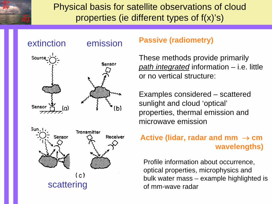
Physical basis for satellite observations of cloud properties (ie different types of f(x)’s)

These methods provide primarily path integrated information – i.e. little or no vertical structure:

Examples considered – scattered sunlight and cloud ‘optical’properties, thermal emission and microwave emission

Passive (radiometry)extinction emission

scattering

Active (lidar, radar and mm → cmwavelengths)

Profile information about occurrence, optical properties, microphysics and bulk water mass – example highlighted is of mm-wave radar

Most cloud & precipitation retrievals are single sensor & ‘physics’ centric – leaving us to ponder which of the seemingly myriad of different approaches is optimal, how accurate is the retrieved information and what is to be gained in combining different types of measurements ?

The future is perhaps with multi-sensor ‘assimilation ‘ of information as, for example, exemplified by the upcoming A-Train

One of the messages conveyed in this overview

0.0

0.2

0.4

0.6

0.8

1.0

0.5 1.0 1.5 2.0 2.5 3.0 3.5 4.0

Sph

eric

al A

lbed

o

Wavelength (µm)

cτ (0.75 µm) = 16

re = 4 µm

re = 8 µm

re = 12 µm

re = 16 µm

re = 20 µm

re = 20 µm + vapor

MODIS Atmosphere Bands

Reflectance variations at these wavelengths →optical depth variations

Cloud optics and ‘microphysics’ : solar scattering

Reflectance variations at these wavelengths → optical depth and re variations

CH. 1

CH

. 2erLWP τ

32

→

(τ,re)

Twomey & Cocks, 1980’sNakajima & King, 1990s

Optical properties

An example: MODIS optical property information

There are three different archived MODIS re products and these are compared to a fourth developed by us at CSU –the differences between them are substantial and beyond our estimated error

Particle Size retrieval examples – low level water clouds

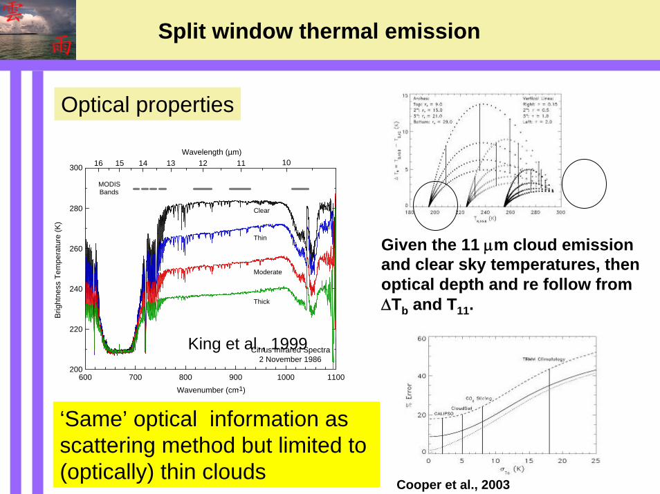
Given the 11 μm cloud emission and clear sky temperatures, then optical depth and re follow from ΔTb and T11.

Cooper et al., 2003

Split window thermal emission

Wavenumber (cm-1)

200

220

240

260

Brig

htne

ss T

empe

ratu

re (K

)

280

300

600 700 800 900 1000 1100

10111213141516Wavelength (µm)

Cirrus Infrared Spectra 2 November 1986

MODIS Bands

Clear

Thin

Moderate

Thick

King et al., 1999

Optical properties

‘Same’ optical information as scattering method but limited to (optically) thin clouds

There is no real attempt to achieve a level of ‘consistency’between different retrieval schemes even using

measurements from the same instrument

Cooper et al., 2005)

Microwave spectrumaround the 22 GHZ water vapor absorption line( )( )

22 oxH/rV/lSw

Wk*/

wkw

*/

Tr)RR(TTlnwkWk

e~ee~e w

−Δμ

=+

−μτ−

−μτ−

l

ll

Measurement of ΔT at two frequencies (19GHz, 37 GHz), estimation of RV/H+ Δkw/l, and Trox allows for simultaneous solution for w and W,

Microwave emission –cloud liquid water path

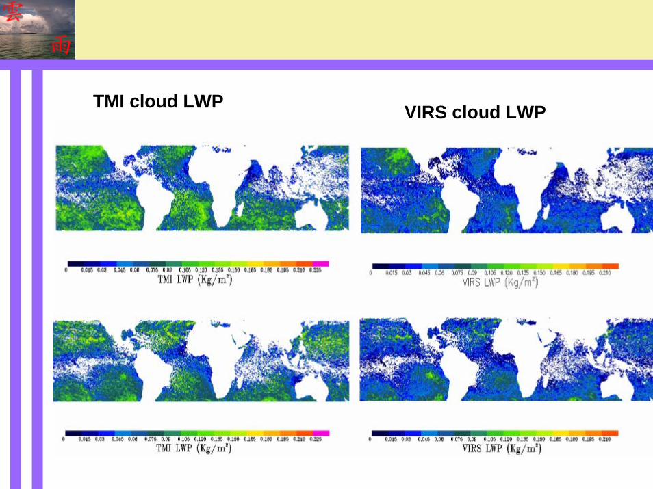
TMI cloud LWP VIRS cloud LWP

Power returned to radar after being scattered from cloud volume is related directly to size of particles in the volume

For a hypothetical cloud (particles allthe same size), the power returned

is proportional to the square of the water and ice content of the (radar) volume

BUT

For real cloud (particles in the volume range insize), the power returned (or Z) is approximatelyproportional to the square of the water and ice content of the (radar) volume.

( )26 6 30 0( )Z n D D dD N D N D= → →∫

Active systems: the mm radar (e.g. CloudSat)

Radar

ln w

ln re

opticaldepth

ln re

ln w

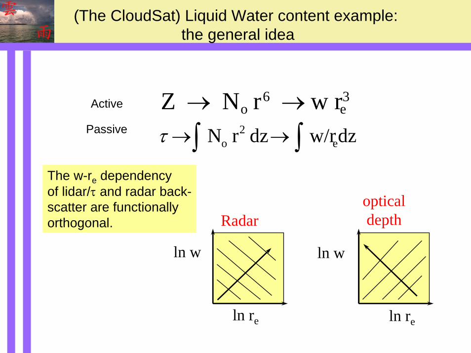
The w-re dependency of lidar/τ and radar back-scatter are functionallyorthogonal.

(The CloudSat) Liquid Water content example: the general idea

Z N r w ro 6

e3→ →dzw/r dz r N e

2o ∫∫ →→τ

Active

Passive

Derived quantities Fractional Uncertainties

re

LWC

LWP

Austin and Stephens, 2001;Austin et al., 2005

No drizzle No drizzle

There is a significant bias in the TMI LWP information (→30%) compared to

VIRS

Courtesy Greenwald and Christophermicrowave

‘opt

ical

’

‘CloudSat algorithm’

‘CloudSat algorithm’ mic

row

ave

‘opt

ical

’

Cloud Liquid Water Path

Stereo example from

The next dimension -adding vertical resolution

AVHRR Multi-layer Cloud Detection Approach

• For single layer clouds, radiative transfer simulation show that as optical depth increase beyond 2, the 11 – 12 micron brightness temperature decreases and approaches an asymptotic value

• Multi-layer clouds exhibit a relationship that can not be modeled (or confused) assuming single layer clouds.

Low Level Water CloudHigh Level Ice CloudCirrus over water cloud (τ = 10)

Courtesy Heidinger & colleagues

• Raining Cloud, mostly, Re_top<Re_base

• Re_top>Re_base could happen for raining cloud because of the non-raining part within the pixel

• For non-raining cloud, mostly R_top>R_bot

• R_top<R_bot could happen for raining cloud because the cloud particle is too small to form rain or the rainfall is too weak for microwave detection

Particle size ‘profile’ retrieval

Chang & Li, 2002;2003

MODIS Retrieved Cloud-top and Cloud-bottom re and TRMM Rainfall Data

Cloud-top re

TRMM rainfall rateCloud-bottom re

Chang & Li, 2002,2003

Model evaluation

Model vs. HIRS 11 μm window (K)

HIRS 11μm window (K)

NOAA-1101/1990 PM orbits(~14:00 LT)

Obs

ERA-40

Recent comparison

15 November 2004

1200 UTOLR

ALBEDO

Model cloud errors can easily be distinguished. Near-real time comparisons are valuable for a wide range of other studies (e.g. outbreaks of Saharan dust)

GERB NWP model

Slingo et al, 2005

Model-observation comparison

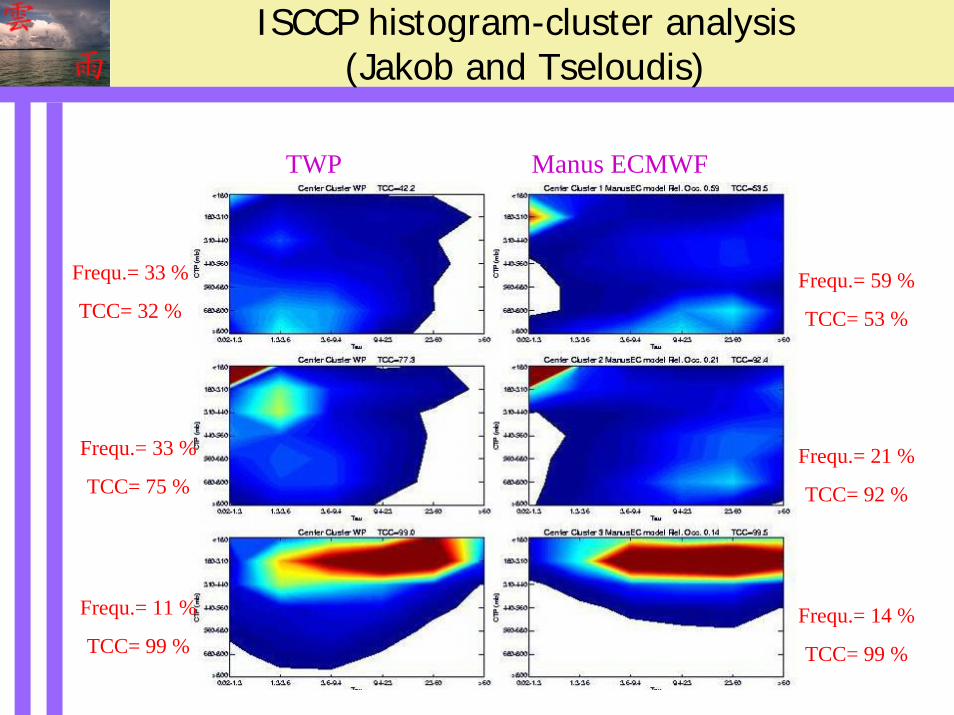
ISCCP histogram-cluster analysis (Jakob and Tseloudis)

TWP Manus ECMWF

Frequ.= 33 %

TCC= 32 %

Frequ.= 33 %

TCC= 75 %

Frequ.= 11 %

TCC= 99 %

Frequ.= 59 %

TCC= 53 %

Frequ.= 21 %

TCC= 92 %

Frequ.= 14 %

TCC= 99 %

Example of the use of orbit data for evaluatingNWP model predicted cloudiness

ECMWF/LITE correlative study Statistics for 60+ LITE Orbits, ±1 bin horizontal and verticalHit Rate = fraction cloudy+clear correctly forecast, =0.896Threat Score = fraction of cloud points correctly forecast = 0.714Probability of Detection = ratio of cloud hits to total # of obs

clouds = 0.796False Alarm rate = rate of forecasting cloud when clear = 0.126

Miller et al., 2000,GRL

Assessment of forecasts of this nature, even just in terms of quantifying cloud occurrence model errors, is presumably an important first step toward eventual assimilation of cloud data.

Many satellite measurements offer redundant information about clouds and precipitation. This is good for the purpose of cross-comparing information as a step to validating knowledge but we cannot be confident about knowing if we are approaching a truth and we have not articulated a clear path to do so.

There is generally little rigor in uncertainty analysis attached to cloud products (if it exists at all), mostly because uncertainties are difficult to validate. This leads to many problems:

• We cannot make meaningful judgments about which of the different approaches is most accurate,

• We have little basis for arguing for small changes in key parameters as being real (e.g. cloud trends)

• We cannot determine the value of combining different measurements such as from multi-sensor observing systems,

• We cannot meaningfully assimilate the observations into dynamical systems

Summary

As we enter an era of the grand challenge, an era of multi-sensor integration and data assimilation, it becomes essential that we develop tools that:

1. Determine more precisely what information resides in measurements of different types as a step to better use of them,

2. Optimally mix information from multiple sources of measurements, and

3. Convert this optimal information to knowledge through (at a minimum) quantification and validation of errors

NW

P co

ntri

butio

n to

clo

ud&

rel

ated

scie

nce

low

high

1960s 1980sAdiabatic Diabatic

This is a period of great optimism but much is left to be done.

…. Well, I think one could always devote more effort. Effort by itself isn’t enough, I think inspiration is also important!

Charney to Platzmann

Better NWP cloud predictions →richer assimilation →more rigorous test of knowledge

By mid 2005, we expect to have a wide range of different sensors, active and passive, optical, infrared and microwave, hyper-spectral to coarse band, all approximately viewing Earth at the same time.

We are left to pose a strategy that optimally combines these measurements, converting them to meaningful information with

verified uncertainties.

Backup

Rain retrieval

4D-Var analysis

Observed Radiances

Model FGT, q

Model FGT, qCloud water + icerain + snow

4D-Var analysis

1D-VarRetrievals of TCWV

Radiative transferFG ‘rainy radiance’

Observed Radiances

(TMI , SSM/I)

Alternative approaches for assimilation of rain information

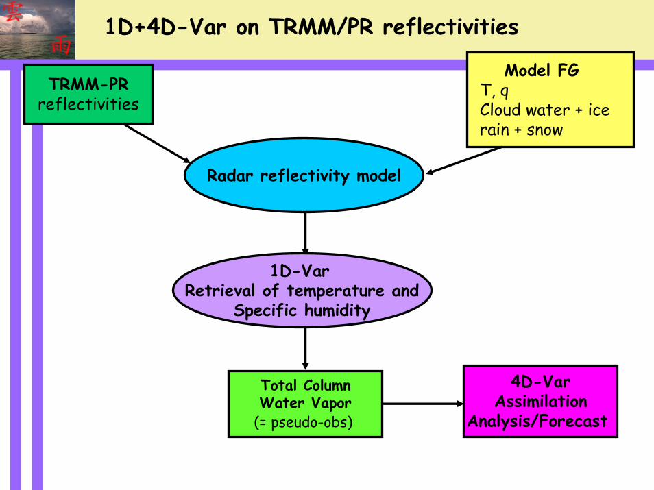
Total ColumnWater Vapor

(= pseudo-obs)

Model FGT, qCloud water + icerain + snow

Radar reflectivity model

1D+4D-Var on TRMM/PR reflectivities

1D-VarRetrieval of temperature and

Specific humidity

TRMM-PRreflectivities

4D-Var Assimilation

Analysis/Forecast

1D-Var retrievals using PR reflectivities with different error assumptions on PR-Z

173OE 174OE 175OE 176OE 177OE 178OE13OS 12OS 11OS 10OS 9OS

400

500

600

700

800

900

TRMM PR reflectivity (dBZ)

15

20

22.5

25

27.5

30

32.5

35

37.5

40

45

173OE 174OE 175OE 176OE 177OE 178OE13OS 12OS 11OS 10OS 9OS

400

500

600

700

800

900

-0.5

- 0.2

-0.2

0.2

0.2

0.2

0.2

0.2

0.2

0.2

0.2

0.2

0.2

0 .20 .2

0.2

0.2

0.2

0.2

0 .2

0 .20.2

0.2

0.2

0.5

0.5

0.5

0.5

0.5

0.5

0 .50.5

0.5

0.5

0.5

0.5

0.5

0.5

0.5

0.5

11

1

1

1 1

1 1

1 1

2

2

2

2

2

3 3

Model reflectivity (dBZ) and humidity increments (g/kg) err=constant 25%, all levels

15

20

22.5

25

27.5

30

32.5

35

37.5

40

45

173OE 174OE 175OE 176OE 177OE 178OE13OS 12OS 11OS 10OS 9OS

400

500

600

700

800

900

0.2

0.2

0 .2

0.2

0.2

0 .2

0.20.2

0.2

0.2

0.2 0.2

0.2

0.2

0.2

0.2

0.2

0 .2

0.2

0.2

0 .2

0.2

0.2

0.50.5

0.5

0.5

0.5

0.5

0.5

0.5

0.5

0.5

0.5

0.5

0.5

0.5

0.5

0.5

0.5

1

1

1

1

1

1

1 1

1

1

1

1

2

2

2

2

Model reflectivity (dBZ) and humidity increments (g/kg) err=constant 50%, all levels

15

20

22.5

25

27.5

30

32.5

35

37.5

40

45

173OE 174OE 175OE 176OE 177OE 178OE13OS 12OS 11OS 10OS 9OS

400

500

600

700

800

900

Model reflectivity (dBZ) fist guess

15

20

22.5

25

27.5

30

32.5

35

37.5

40

45

1D-Var 25% error at all levels

1D-Var 50% error at all levels

173OE 174OE 175OE 176OE 177OE 178OE13OS 12OS 11OS 10OS 9OS

400

500

600

700

800

900

-0.2

-0.20.2

0.2

0.2

0.2

0.2

0.2

0.2

0.2

0.2

0.2

0.2

0.2

0.2

0.5

0.5

0.5

0.5

0.5

0.5

0.5

0.5

0.5

0.5

0.5

0.5

1

1

1

1

1

1

1

2 2

2 2

Model reflectivity (dBZ) and humidity increments (g/kg) err=constant 25%, level 28 only

15

20

22.5

25

27.5

30

32.5

35

37.5

40

45

1D-Var retrievals using PR reflectivities: observations at one level only vs full profile

173OE 174OE 175OE 176OE 177OE 178OE13OS 12OS 11OS 10OS 9OS

400

500

600

700

800

900

TRMM PR reflectivity (dBZ)

15

20

22.5

25

27.5

30

32.5

35

37.5

40

45

173OE 174OE 175OE 176OE 177OE 178OE13OS 12OS 11OS 10OS 9OS

400

500

600

700

800

900

-0.5

- 0.2

-0.2

0.2

0.2

0.2

0.2

0.2

0.2

0.2

0.2

0.2

0.2

0 .20 .2

0.2

0.2

0.2

0.2

0 .2

0 .20.2

0.2

0.2

0.5

0.5

0.5

0.5

0.5

0.5

0 .50.5

0.5

0.5

0.5

0.5

0.5

0.5

0.5

0.5

11

1

1

1 1

1 1

1 1

2

2

2

2

2

3 3

Model reflectivity (dBZ) and humidity increments (g/kg) err=constant 25%, all levels

15

20

22.5

25

27.5

30

32.5

35

37.5

40

45

173OE 174OE 175OE 176OE 177OE 178OE13OS 12OS 11OS 10OS 9OS

400

500

600

700

800

900

Model reflectivity (dBZ) fist guess

15

20

22.5

25

27.5

30

32.5

35

37.5

40

45

1D-Var obs at all levels

1D-Var obs at level 48 (~2km)

15°S 15°S

10°S10°S

170°E

170°E 175°E

175°E

TCWV increments (kg/m2) .ec09.25r4.pr.hpca.0.2_Allkg/m2

-25-20

-10

-5

-3

-2-1

1

23

5

10

20

25

20°S 20°S

10°S10°S

0° 0°

170°E

170°E 180°

180°TCWV guess .ec09.25r4.pr.hpca.0.2_Allkg/m2

20

25

30

35

40

45

50

55

60

65

70

75

TCWV guess (kg/m^2)

Background and 1D-Var increments of Total Column Water Vapour (pseudo-obs for 4D-Var)

Increments indicate an overall moistening confined along the satellite track

TCWV increments (kg/m^2)

168E 170E 172E 174E 176E

168E 170E 172E 174E 176E

18S

16S

14S

12S

10S

18S

16S

14S

12S

10S

0 6

12 18 24

36 48

60

72

84

96

108

OBSCONTROLPR-REFLPR-RAINTMI-RAINTMI-TB

ZOE TRACK FORECAST (BASE: 2002122612)

-As suggested by the MSLP changes, the track forecasts are substantially improved when TRMM observations are assimilated in rainy areas.

-Despite the smaller spatial coverage of TRMM/PR data (200-km swath) compared to that of TMI data (780-km swath), the impact of both types of observations is comparable.

Comparison of track forecasts (started on 26 December 2002 at 1200 UTC) obtained from the control, two TRMM/PR, and two TMI experiments to the observed track.

Concluding comments:

1. The assimilation methods pioneered at the Centre represents an important a bridge linking the traditional factions of the sciences.

2. While assimilation of data on quantities characterized as smooth and continuous, we are now entering a period of assimilation of hydrological parameters

And then, of course, there remains, even in the short-range problem, I think, the physical factors, which are still not adequately understood. The matter of the boundary layer and precipitation process …. Charney to Platzmann

1980

1970The first phase: the

period of great imagination The first 24hr view of global clouds

TIROS-9, February 13, 1965

The launch of TIROS-1, April 1960

2000The third phase: grand

challenge to create ‘knowledge’

Decadal cloud amount trends, precipitation variability

Assimilation of precipitation andcloud radiances

(Heidinger poster)

1990

The second phase: the period of great

information-gathering

1. Global climatologiesof cloud occurrence*, optical properties, 1983-present * Cloud mask/

identification /screeningFirst flight of back-scatter lidar, LITE, 1996

First flight of precipitation radar, TRMM, 1997

Aqua, CO2 slicing AVHRR, split window

MODIS-AVHRR comparisons: Hurricane Ivan

Courtesy, Heidinger

We use different techniques based on the same physics (e.g. emission and scattering) for arriving at the same information

Example application: Aircraft Contrail Detection

““RacetrackRacetrack””flight patternflight pattern

Coutesy S. Miller

CloudSat Examples1. Illustrating simple ideas of Information content

Information is an augmentation of existing knowledge

P(xa) Sa

P(x⏐y) Sx

Therefore we might think that the measurement has added information if the ‘volume’ of the distribution is reduced

Shannon total information)]([)]([ xPsxPsH a −=

The observing system identifies 2H states over and above our background knowledge. It is a measure of system resolution.

MODIS ice cloud optical properties IWP~100

Re=16Ht=9km

IWP~100Re=16Ht=14km

Hi

The point about this is there is no one optimal combination of channels – the combination of channels varies according to conditions

Hi

Cooper et al., 2004

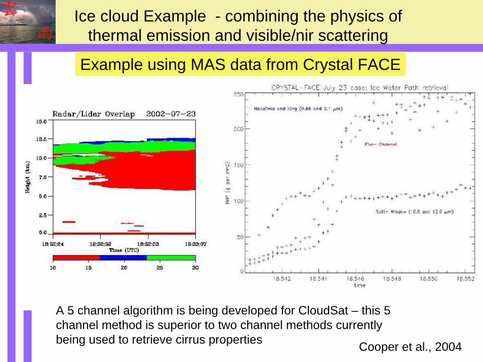
Example using MAS data from Crystal FACE

A 5 channel algorithm is being developed for CloudSat – this 5 channel method is superior to two channel methods currently being used to retrieve cirrus properties Cooper et al., 2004

Ice cloud Example - combining the physics of thermal emission and visible/nir scattering

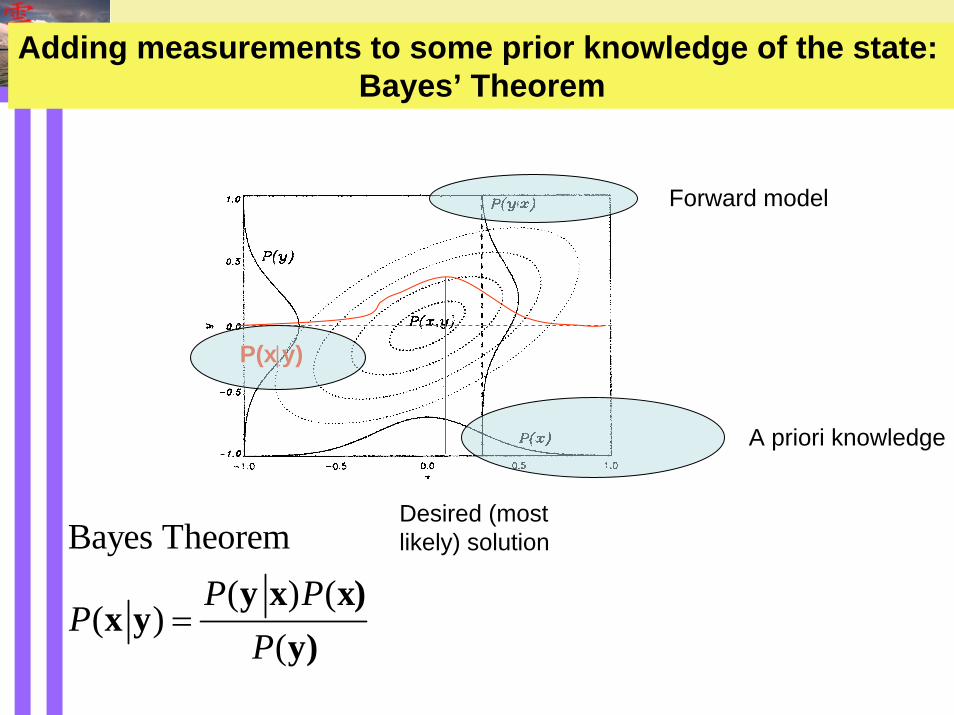
Bayes Theorem( ) (

( )(

P PP

P=

y x x)x y

y)

Forward model

Adding measurements to some prior knowledge of the state: Bayes’ Theorem

A priori knowledge

P(x|y)

Desired (most likely) solution

3. Error Validation

The CloudSat validation goal is to confirm the retrieval error estimates provided by all algorithms- ground truth when possible (ISO GUM*, method A) - component analyses (ISO GUM, method B)- consistency analyses (ISO GUM, method B)

RMS~30%

Total errors derived from actual comparison of retrieved with in situ, method A

* International Organization for Standards (ISO) Guide to the expression of uncertainty in Measurements

As we add channels, we can see how information is increased and how retrieval errors are reduced.

Ice cloud Example - combining the physics of thermal emission and visible/nir scattering

Passive:Passive:EngelenEngelen and Stephens, 1997, JGR,6929and Stephens, 1997, JGR,6929--6939 6939 (ozone)(ozone)HeidingerHeidinger and Stephens, 1998; 2000,J.Atmos.Sci.,57and Stephens, 1998; 2000,J.Atmos.Sci.,57,(cloud),(cloud)Miller, Austin and Stephens, 2001,JGR,106,17981Miller, Austin and Stephens, 2001,JGR,106,17981--17995 17995 (cloud)(cloud)Cooper, Cooper, LL’’EcuyerEcuyer and Stephens,2003, JGR,108and Stephens,2003, JGR,108,(cloud),(cloud)Engelen et al., 2002; COCO22

PassivePassive--PassivePassiveEngelenEngelen and Stephens,1999;QJRMS,125,331and Stephens,1999;QJRMS,125,331--351; 351; water vaporwater vaporChristi and Stephens, 2004;JGR; Christi and Stephens, 2004;JGR; COCO22

Active Active -- Passive:Passive:Stephens, Stephens, EngelenEngelen, Vaughan and Anderson,2001,JGR, , Vaughan and Anderson,2001,JGR, (aerosol/cloud)(aerosol/cloud)Austin and Stephens, 2001, Austin and Stephens, 2001, JGRJGR, , 106106, 28,233 , 28,233 -- 28,242)28,242) (cloud).(cloud).LL’’EcuyerEcuyer and Stephens, 2002, and Stephens, 2002, J.ApplJ.Appl. Met., 41,271. Met., 41,271--285 285 ((precipprecip).).Benedetti, Stephens and Haynes, 2003; JGR, 108 Benedetti, Stephens and Haynes, 2003; JGR, 108 (cirrus)(cirrus)Austin and Stephens, 2004; JGR submitted Austin and Stephens, 2004; JGR submitted (cloud)(cloud)MitrescuMitrescu, Haynes,Stephens, , Haynes,Stephens, HeymsfieldHeymsfield and McGill, 2004 and McGill, 2004 (cirrus)(cirrus)

Information Content:Information Content:EngelenEngelen and Stephens, 2003, and Stephens, 2003, J.Appl.MetJ.Appl.Met..LL’’EcuyerEcuyer, Cooper, , Cooper, Leesman,,StephensLeesman,,Stephens, 2004; In preparation. , 2004; In preparation. Cooper, et al., 2004; in preparation Cooper, et al., 2004; in preparation LabonnoteLabonnote and Stephens, 2004;JGRand Stephens, 2004;JGR

Bayes Theorem( ) (

( )(

P PP

P=

y x x)x y

y)

Forward model

Adding measurements to some prior knowledge of the state: Bayes’ Theorem

A priori knowledge

P(x|y)

Desired (most likely) solution

Example: Return to our ‘simple’ example and apply Optimal Estimation technique

( ) ( )11 1 1 1 1.05ˆ

0.95T T

y a y a a

−− − − − ⎛ ⎞= + + = ⎜ ⎟

⎝ ⎠x K S K S K S y S x

1.2ˆ

1.1a⎛ ⎞

= ⎜ ⎟⎝ ⎠

xA priori assumption

Assume diagonal covariance matrices with 0.001 for the errorin the measurements and 0.5 for the error in the a priori guess.

We also obtain a covariance matrix for the result:

( ) 11 1 0.25 0.250.25 0.25

Tx y a

−− − −⎛ ⎞= = ⎜ ⎟−⎝ ⎠

S K S K + S

So what have we gained???

Assume NT and σlog

are constant in height

The CloudSat Liquid Water content example

Measurements vector

m = p+1 elements

State vector

n = p+2 elements

“forward model” f(x,b)

A priori vector

p+2 elements

Application to ARM data

Old with width parameter specified New with width parameter retrieved

Passive:Passive:EngelenEngelen and Stephens, 1997, JGR,6929and Stephens, 1997, JGR,6929--6939 6939 (ozone)(ozone)HeidingerHeidinger and Stephens, 1998; 2000,J.Atmos.Sci.,57and Stephens, 1998; 2000,J.Atmos.Sci.,57,(cloud),(cloud)Miller, Austin and Stephens, 2001,JGR,106,17981Miller, Austin and Stephens, 2001,JGR,106,17981--17995 17995 (cloud)(cloud)Cooper, Cooper, LL’’EcuyerEcuyer and Stephens,2003, JGR,108and Stephens,2003, JGR,108,(cloud),(cloud)Engelen et al., 2002; COCO22

PassivePassive--PassivePassiveEngelenEngelen and Stephens,1999;QJRMS,125,331and Stephens,1999;QJRMS,125,331--351; 351; water vaporwater vaporChristi and Stephens, 2004;JGR; Christi and Stephens, 2004;JGR; COCO22

Active Active -- Passive:Passive:Stephens, Stephens, EngelenEngelen, Vaughan and Anderson,2001,JGR, , Vaughan and Anderson,2001,JGR, (aerosol/cloud)(aerosol/cloud)Austin and Stephens, 2001, Austin and Stephens, 2001, JGRJGR, , 106106, 28,233 , 28,233 -- 28,242)28,242) (cloud).(cloud).LL’’EcuyerEcuyer and Stephens, 2002, and Stephens, 2002, J.ApplJ.Appl. Met., 41,271. Met., 41,271--285 285 ((precipprecip).).Benedetti, Stephens and Haynes, 2003; JGR, 108 Benedetti, Stephens and Haynes, 2003; JGR, 108 (cirrus)(cirrus)Austin and Stephens, 2004; JGR submitted Austin and Stephens, 2004; JGR submitted (cloud)(cloud)MitrescuMitrescu, Haynes,Stephens, , Haynes,Stephens, HeymsfieldHeymsfield and McGill, 2004 and McGill, 2004 (cirrus)(cirrus)

Information Content:Information Content:EngelenEngelen and Stephens, 2003, and Stephens, 2003, J.Appl.MetJ.Appl.Met..LL’’EcuyerEcuyer, Cooper, , Cooper, Leesman,,StephensLeesman,,Stephens, 2004; In preparation. , 2004; In preparation. Cooper, et al., 2004; in preparation Cooper, et al., 2004; in preparation LabonnoteLabonnote and Stephens, 2004;JGRand Stephens, 2004;JGR

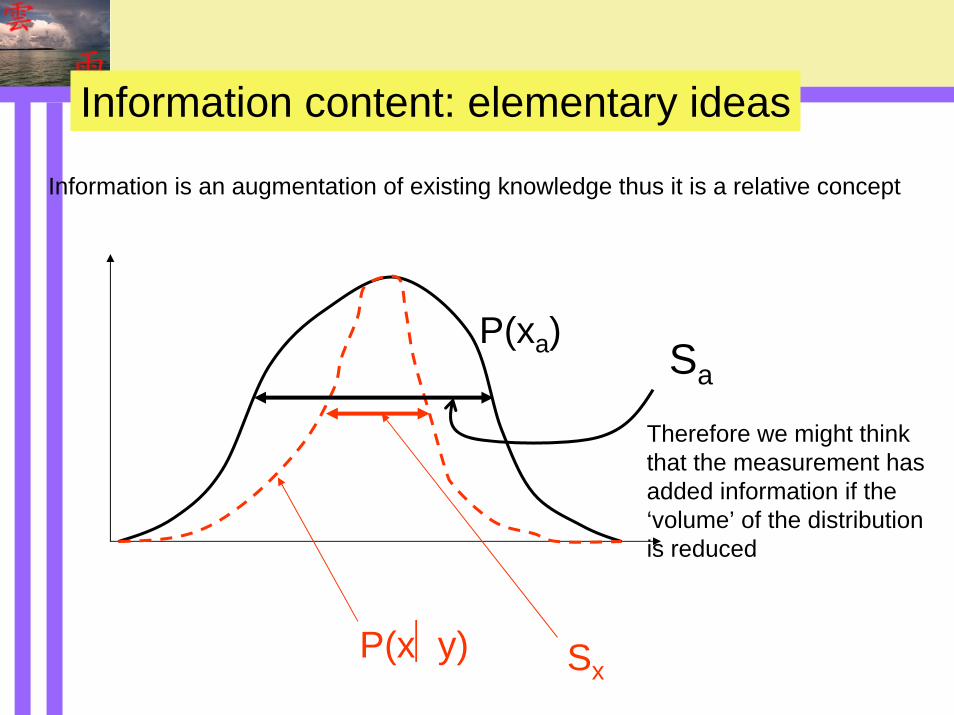
Information content: elementary ideas

Information is an augmentation of existing knowledge thus it is a relative concept

P(xa) Sa

P(x⏐y) Sx

Therefore we might think that the measurement has added information if the ‘volume’ of the distribution is reduced

Shannon’s measure of informationEntropy is a measure of the # of distinct states of a system, and thus a measure of information about that system. If the system is defined by the pdf P(x), then

( ) ( ) ln ( )

forP(x) exp[-(x- x ) (x- x )]

1( ) ln2

Tx

x

s P k P x P x dx

S

s P S

= −

→

=

∫

In our context, information is the change (reduction) in entropy of the ‘system’ after a measurement is made

1

( ( )) ( ( ))1 ln2

a

a x

H s P x s P x

H S S −

= −

=

j

iij

ay

xa

xfK

KSSK

SSITrdfs

H

A

∂∂

=

=

−=

−

−

2/12/1

1

~

)( # of measurements above noise

Singular values of this scaled Jacobean matrix above unity tell us about how many pieces of information are contained in the measurements. The singular vectors tell us what combination of state parameters are retrievable

Summary of information properties

Property Interpretation

The observing system identifies 2H states over and above our background knowledge. It is a measure of system resolution.

Provides a measure of where information comes to produce the retrieved state x