Satellite System and Sensors Satellite System and Sensors Part II Part II Low to Moderate Optical and Low to Moderate Optical and Radar Satellites Radar Satellites Dr. Dr. Kiyoshi Honda Kiyoshi Honda Space Technology Applications and Research Program School of Advanced Technologies Asian Institute of Technology Low to Moderate Resolution Optical Satellites Low to Moderate resolution satellite data with their resolution of 250 to 1km is important to regional to global scale environmental monitoring. The advantage of these data are their frequent observation which covers the whole globe within one day. Some satellites have morning and afternoon satellites which gives us twice a day observation. In spite of its low spatial resolution, its high multi-temporal capability, high-sensitivity sensors, multi-spectral capability provide us with excellent data and application opportunity. Also, recent effort to provide the data in systematic way such as distribution on internet, producing value added data has been enhancing its usability.
Transcript
1
Satellite System and SensorsSatellite System and SensorsPart IIPart IILow to Moderate Optical and Low to Moderate Optical and Radar SatellitesRadar Satellites
Dr. Dr. Kiyoshi HondaKiyoshi Honda
Space Technology Applications and Research ProgramSchool of Advanced TechnologiesAsian Institute of Technology
Low to Moderate Resolution Optical Satellites
Low to Moderate resolution satellite data with their resolution of 250 to 1km is important to regional to global scale environmental monitoring.The advantage of these data are their frequent observation whichcovers the whole globe within one day. Some satellites have morning and afternoon satellites which gives us twice a day observation.In spite of its low spatial resolution, its high multi-temporal capability, high-sensitivity sensors, multi-spectral capability provide us with excellent data and application opportunity.Also, recent effort to provide the data in systematic way such as distribution on internet, producing value added data has been enhancing its usability.
Series of algorithm for estimating environmental physical parameter.
Local Receiving is feasibleFree for receivingS band – X band100,000 US$-500,000US$
Hyper-Spectral Information e.g. 36 ch.Improved Resolution to 250m-500mValue Added Data Product, e.g. MODISNetwork Data Distribution, AIT, UT, NASANear Real time Monitoring, several hrs.
Advantage of High-Resodata from previous LectureHigh-Resolution
Easy for interpretation
Good products lineSystematicHigh-Precision
Good search/ordering system
Commercial Distributor
Easy HandlingCommon formatsSupported by various softwareGood combination with 1/100,00 –1/50,000 mapsPlenty of Application examples
Improved resolutionMulti-Spectral
Limitation Limitation of High-Resodata from previous LectureRe-Visit Time
2 – 18 daysCloud Cover
Project planningSpectral Information
Panchromatic to several bands only
S/NNormally 6-8 bits
Geo-locationDistortion by topographic effect ( edge, high-mountains )Off-Nadir Observation
CoverageSeveral 10km –180km
CostUsually not freeSometimes expensiveSuper-high reso: Expensive
Satellite Geometry Model: sometimes not open
Spatial ResolutionGeo-locationData Handling
Format: Local formatNot enough Support from commercial softwareProjection10bits data
Difficulty in implementing local processing systemOff-Nadir Observation
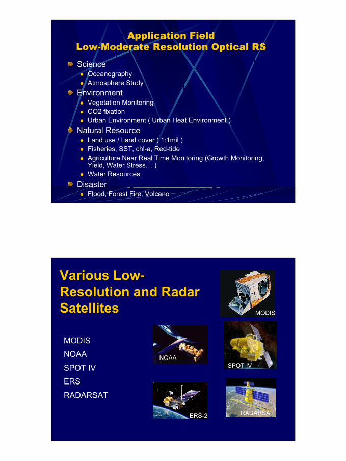
Natural ResourceLand use / Land cover ( 1:1mil )Fisheries, SST, chl-a, Red-tideAgriculture Near Real Time Monitoring (Growth Monitoring, Yield, Water Stress… )Water Resources
DisasterFlood, Forest Fire, Volcano
Various LowVarious Low--Resolution and Radar Resolution and Radar SatellitesSatellites
MODIS
NOAA
SPOT IV
ERS
RADARSAT
MODIS
NOAASPOT IV
ERS-2 RADARSAT
4
High-Reso SatelliteQuick Bird 0.62m
Low-Reso, High-TemporalNOAA/AVHRR 1 km
Trade-off in PerformanceSpatial Resolution ( 1 observation unit on ground surface )
30 m - 250km - 1km
Temporal Resolution16 days - 1day
Spectral Resolution7 channel vs 36 channel
Observation Extent185 km vs 2,300km
S/N8bits vs 10bits
cost1 scene 800US$ vs Free ( Broadcast )
5
0.4 0.6 0.8 1.21.0 1.4 1.6 1.8 2.0 2.2 2.4 2.6
20
40
50
60
70
80
10
0
Vegetation
Soil
Clear River Water Turbid River Water
Wavelength (µm)
Perc
ent R
efle
ctan
ce
30
Spectral ReflectanceSpectral Reflectance
NDVI: Normalized Differential Vegetation Index
NDVI = (NIR - VR)/(NIR+VR) = tanα = y'/x'
NIR
VR
α NIR = VR NDVI = 0
NDVI=1.0
NDVI= -1.0
θ
forestbare land
x'
y'
x'y'
= cos π/4 sin π/4– sin π/4 cos π/4
VRNIR
tan α =y'x' = NIR – VR
NIR + VR
6
EOS ( Earth Observing System ) - A Project by NASA15 years earth observation for Environmental ProblemsWith International Collaboration; Japan, Canada, …
Series of Afternoon and Morning SatellitesEOS-AM1, EOS-PM1, EOS-AM2, EOS-PM2
TERRA ( EOS-AM1)Successfully launched on December 18, 1999Activated for science operations on Feb. 24, 2000
Followed by AQUA(EOS-PM1) in 2002
5 Instruments on TERRA
MODIS (Moderate-resolution Imaging Spectroradiometer : USA)
ASTER (Advanced Spaceborne Thermal Emission and Reflection Radiometer : Japan )
CERES (Clouds and the Earth's Radiant Energy System: USA)
MISR (Multi-angle Imaging Spectro-Radiometer: USA)
MOPITT (Measurements of Pollution in the Troposphere: Canada)
7
Moderate Resolution250m Resolution
Hyper Spectral36 discrete spectral bands.
High Multi-TemporalSees every point on our world every 1-2 days
Successor of Very Popular NOAA/AVHRRNOAA/AVHRR: 1km - 5 Channels – Morning and Afternoon
MODIS is ideal for Global – Regional Environment Monitoring by improving capability of NOAA/AVHRR
250m(bands 1-2)500m(bands 3-7)1000m(bands 8-36)
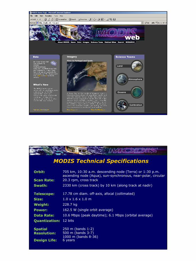
MODIS (or Moderate Resolution Imaging Spectroradiometer) is a key instrument aboard the Terra (EOS AM) and Aqua (EOS PM) satellites. Terra's orbit around the Earth is timed so that it passes from north to south across the equator in the morning, while Aqua passes south to north over the equator in the afternoon. Terra MODIS and Aqua MODIS are viewing the entire Earth's surface every 1 to 2 days, acquiring data in 36 spectral bands, or groups of wavelengths (see MODIS Technical Specifications). These data will improve our understanding of global dynamics and processes occurring on the land, in the oceans, and in the lower atmosphere. MODIS is playing a vital role in the development of validated, global, interactive Earth system models able to predict global change accurately enough to assist policy makers in making sound decisions concerning the protection of our environment.
8
Orbit: 705 km, 10:30 a.m. descending node (Terra) or 1:30 p.m. ascending node (Aqua), sun-synchronous, near-polar, circular
Scan Rate: 20.3 rpm, cross track
Swath: 2330 km (cross track) by 10 km (along track at nadir)
Telescope: 17.78 cm diam. off-axis, afocal (collimated)
Size: 1.0 x 1.6 x 1.0 m
Weight: 228.7 kg
Power: 162.5 W (single orbit average)
Data Rate: 10.6 Mbps (peak daytime); 6.1 Mbps (orbital average)
Quantization: 12 bits
Spatial Resolution:
250 m (bands 1-2)500 m (bands 3-7)1000 m (bands 8-36)
Design Life: 6 years
MODIS Technical Specifications
9
Primary Use Band Bandwidth Spectral Radiance Required SNR
MODIS Standard ProductsThere are 44 products, Some are validated, some are not
validated.Data Products
There are 44 standard MODIS data products that scientists are using to study global change. These products are being used by scientists from a variety of disciplines, including oceanography, biology, and atmospheric science. This section details each product individually, introducing you to the products, explaining the science behind them, and alerting you to known areas of concern with the data products. Also documented is each of the product's latest availability information. To view specific info on a product, select it from the menu below.
Calibration 3 ( Radiance Counts, Calibrated Geolocated Radiances, Geolocation Data set )
( Water Leaving Rad, Pigment Concen. Chl-Fluorescence, Chl-a, PAR, SS, Organic Matter, Coccolith, Ocean Water Attenuation, Ocean Primary Prod., SST, Phycoerythrin Cocent., Total Absorption Coeff., Ocean Aerosol, Clear Water Eps. )( http://modis.gsfc.nasa.gov/data/dataproducts.html )
MODIS Standard Products & its levelBeta Products
Beta Products are minimally validated, early release products that enable users to gain familiarity with data formats and parameters. Product is probably not appropriate as the basis for quantitative scientific publications.
Provisional ProductsProvisional Products are partially validated and improvements are continuing. Provisional products are viewed as early science validated products and useful for exploratory and process scientific studies. Quality may not be optimal since validation and quality assurance are ongoing. Users are expected to review products quality summaries before publication of results.
Validated ProductsValidated Products have well defined uncertainties. These are high quality products suitable for longer term or systematic scientific studies and publication. There may be later
I improved versions. Users are expected to review products quality summaries before publication of results.
Stage 1 Validation: Product accuracy has been estimated using a small number of independent measurements obtained from selected locations and time periods and ground-truth/field program efforts.
Stage 2 Validation: Product accuracy has been assessed over a widely distributed set of locations and time periods via several ground-truth and validation efforts.
Stage 3 Validation: Product accuracy has been assessed and the uncertainties in the product well established via independent measurements in a systematic and statistically robust way representingglobal conditions.
11
MODIS for Flood MonitoringMODIS for Flood Monitoring
MODIS for Forest Fire MODIS for Forest Fire MonitoringMonitoring
MODIS has 16 thermal bands and is well suited for hotspots detection.
Band 21 and band 31, which have wavelengths of 3.959nm and 11.03 nm respectively, are used to determine hotpots. The criteria are:
BT21>360K or
BT21>360K and BT21-BT31>20K
Once a pixel is found to be hotspot, it will be marked in red on the georectified MODIS image
MODIS hotspot image on 7 Sep 2001. Riau Province, Sumatra
12
MODIS for Forest Fire MonitoringMODIS for Forest Fire Monitoring
Zoom-in of Riau Province, Sumatra image in 1-km resolution
The fires captured by SPOT1 on the same day
For details visit: http://www.crisp.nus.edu.sg/~research/#current
http://www.noaa.gov/
NOAA
13
NOAANOAA AVHRRAVHRR Feb 1-10, 1999
(Advanced Very High Resolution Radiometer)
AVHRR is primarily used forvegetation studies -the study and monitoring of drought conditions.
14
AIT NOAA/AVHRR - MODIS/TERRAReception, Archiving and Distribution
• NOAA/AVHRR Since 15 November 1997
• TERRA/MODIS Since 25 May 2001• Archiving all of the received data• Produce 10days and Monthly NDVI• Network Data Distribution over Internet for
Near Real Time Environment Monitoring
(Asia Pacific Advanced Network)
between Thailand -Japan
AITAIT
NECTECNECTEC(THAISARN)(THAISARN)
NIINII(SINET)(SINET)
WIDEWIDE
U. TokyoU. Tokyo
JCSATJCSAT1.5Mbps1.5Mbps
Fiber OpticsFiber Optics2Mbps2Mbps2 Mbps
Thailand
APANAPAN
Japan
GISTDAGISTDA
Min. Min. AgriAgriMaffinMaffin
Fire MapFire Map
SE AsiaSE Asia
15
Cloud Free CompositeTo produce cloud free imagesOverlay certain period of imagesDetect Cloud Free PixelsSelect pixels which has not been influenced by clouds among the candidates in the same locationCriteria
Maximum NDVIScan Angle
Popular period10days, 30 days
NDVI 10-days CompositeBangkok(AIT), Ulaanbaator, Tokyo, Kuroshima
16
Global Mapping Project - Ganges River Basin
Create database covering all the land area on the earth’s surface with uniform accuracy and specifications in order to contribute in formulating regional level policies and planning/regional level strategies to resolve environmental problems such as
•soil erosion/land slide hazard
•food security
•desertification etc.,
In this course, Ganges river basin area which covers 35degree N to 20 degree N and 70 degree E to 95 degree E, is being mapped using
•NOAA AVHRR data
•Elevation data
•Precipitation data
•Temperature data
Monthly Composite of NOAA AVHRR-October 1998
17
Unsupervised Classification of Multi-Temporal NDVI Results
Sample 1
Sample 4
Sample 3
Sample 2
Agriculture area
Vegetation IndexVegetation IndexThe ratio of TM Band 4 to Band 3 or AVHRR Bands 2 to 1 is a simple approximation of the Vegetation Index (VI).
A. April 12-May 2, 1982; B. July 5-25, 1982; C. Sept. 27-Oct. 17, 1982; D. Dec. 20, 1982-Jan. 9, 1983. <http://rst.gsfc.nasa.gov/Sect3/Sect3_4.html>
… area
Left image: Use AVHRR to observe seasonal changes in biomass ("green wave") over all of Africa
18
Crop Stress is indicated by progressive decrease in Near-IR reflectance but a reversal in Short-Wave IR reflectance, as shown in this general diagram:
http://rst.gsfc.nasa.gov/Sect3/Sect3 1.html
dry season in normal year
dry season in drought year
8 Apr 1997 20 May 1997 23 Jun 1997 7 Jul 1997
26 Jul 1997 7 Aug 1997 5 Sept 1997 12 Sept 1997
5 Nov 1997 17 Dec 1997 1 Jan 1998 15 Apr 1998
20 May 1998 25 Jun 1998 3 Jul 1998 2 Aug 1998
6 Sept 1998 9 Oct 1998 26 Nov 1998
-0.79 0.54
Vegetation change of NOAA AVHRR by using NDVI
RS for Drought Monitoring(using NOAA AVHRR) in Indonesia
19
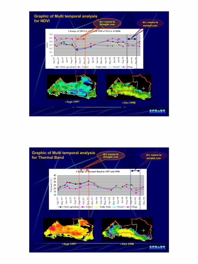
Graphic of Multi temporal analysis for NDVI
Change of NDVI in 1997 and 1998 of NO AA AVHRR
0
0.1
0.2
0.30.4
0.5
0.6
Apr
-97
May
-97
Jun-
97
Jul-9
7
Aug
-97
Sep-
97
Oct
-97
Nov
-97
Dec
-97
Jan-
98
Feb-
98
Mar
-98
Apr
-98
May
-98
Jun-
98
Jul-9
8
Aug
-98
Sep-
98
Oct
-98
Nov
-98
ND
VI
Other agriculture Forest1 Paddy fields Forest2 Village
dry season in drought year
5 Sept 1997
dry season in normal year
9 Oct 1998
Graphic of Multi temporal analysis for Thermal Band
Change of Thermal Band in 1997 and 1998
10152025303540
Apr
-97
May
-97
Jun-
97
Jul-9
7
Aug
-97
Sep-
97
Oct
-97
Nov
-97
Dec
-97
Jan-
98
Feb-
98M
ar-9
8
Apr
-98
May
-98
Jun-
98
Jul-9
8
Aug
-98
Sep-
98
Oct
-98
Nov
-98
Dec
-98
Ther
mal
(o C)
Other agriculture Forest1 Paddy fields Forest2 Village
dry season in drought year
5 Sept 1997
dry season in normal year
9 Oct 1998
20
Flood Monitoring using NOAA
Flood Monitoring in Thailand using NOAA AVHRR Satellite Image
NOAA AVHRR and DEMNOAA AVHRR and DEM
Flight SimulationFlight SimulationBackground for Background for GreenmapGreenmap
21
The VEGETATION instrument on Spot 4 features a wide-field-of-view radiometric imaging instrument operating in four spectral bands (blue, red, near- and short-wave infrared) at a resolution of 1 kilometer; a solid-state onboard recorder able to store 90 minutes of data; image telemetry systems and a computer to manage the instrument's work plan. A dedicated onboard calibration device also monitors radiometric performance of the cameras.
Spot 4-VEGETATION
With a swath width of 2,250 kilometres, the VEGETATION instrument covers almost all of the globe's land masses while orbiting the Earth 14 times a day. Only a few zones near the equator are covered every day. Areas above 35° latitude are seen at least once daily.
Electromagnetic radiationwavelengthλ , frequency ν and the velocityυ have the following relation.
λ = υ/ν
Note: Electro-magnetic radiation has the characteristics of both wave motion and particle motion.
Basic Geometry
28
RADAR Back ScatterSurface Back Scatter
RoughnessVolume Scatter and Target’s Structure
Volume, StructureDielectric Property
MoisturePolarization
Distance
Surface Scattering
29
X-band
C-band
L-band
INTERACTIONS
Penetration intovolume: agriculture
Scattering by Volume & Structure
30
Dielectric Constant
High Dielectric C.(Wet) : High Backscatter
Shown here is a radar image acquired July 7, 1992 by the European Space Agency (ESA) ERS-1 satellite. This synoptic image of an area near Melfort, Saskatchewan details the effects of a localized precipitation event on the microwave backscatter recorded by the sensor. Areas where precipitation has recently occurred can be seen as a bright tone (bottom half) and those areas unaffected by the event generally appear darker (upper half). This is a result of the complex dielectric constant which is a measure of the electrical properties of surface materials. The dielectric property of a material influences its ability to absorb microwave energy, and therefore critically affects the scattering of microwave energy.The magnitude of the radar backscatter is proportional to the dielectric constant of the surface. For dry, naturally occurringmaterials, this is in the range of 3 - 8 , and may reach values as high as 80 for wet surfaces. Therefore the amount of moisture inthe surface material directly affects the amount of backscattering. For example, the lower the dielectric constant, the more incident energy is absorbed, the darker the object will be on the image
This is a three-dimensional view of Isabela, one of the Galapagos Islands located off thewestern coast of Ecuador, South America. This view was constructed by overlaying a Spaceborne Imaging Radar-C/X-band Synthetic Aperture Radar (SIR-C/X-SAR) image on a digital elevation map produced by TOPSAR, a prototype airborne interferometric radar which produces simultaneous image and elevation data.
DEM(II)
This three-dimensional perspective of
Valley in the northern Tibetan Plateau of western China was
createdby combining two spaceborne radarimages using a technique known asinterferometry. Visualizations likethis are helpful to scientists
becausethey reveal where the slopes of thevalley are cut by erosion, as well asthe accumulations of gravel
Soil sample collected at a sampling pointusing a 100-cc core barrel
Soil samples oven-driedfor 24 hours at 105 oC
Quantitative Soil Moisture Measurement Using ERS-2 C-band SAR data in Sukhothai
- Satellite Synchronized Field Survey -
Surface roughness measurement
• A roughness board of 130x45-cm size was used to measure surface roughness.
• First measurement was done during the fallow period (9 May 1998) when the paddy fieldsare assumed to have the smallest root mean square height deviation.
• Second measurement was made during the start of land preparation (6 July 1998) whenthe paddy fields would have their maximum height deviation from the mean.
σ = { 1/ (N-1) [ Σ (zi)2 - N(z)2] }1/2
Where:
z = (1/ N) Σ zi
35
Soil moisture &radar backscatter
-14
-12
-10
-8
-6
-4
-2
0
0 5 10 15 20 25 30 35 40
Vol. SM (%)
back
scat
ter
(dB) 18 18 JulJul
28 28 FebFeb
9 9 MayMay
6 6 SepSep
22 22 AugAug
5 5 DecDec
Radar backscatter plotted against volumetric soil moisture:
Canada – Japan – ThailandWithin 8 hrs after reception
Field locations of reflectors andcorresponding views in the
image(11a) Station No. 1
Reflector: 8.53 dBBackground: -21.22 dB
(11b) Station No. 2
Reflector: 9.89 dBBackground: -2.19 dB
(11c) Station No. 3
Reflector: 9.48 dBBackground: -3.14 dB
(11d) Station No. 4
Reflector: 9.21 dBBackground: -5.08 dB
for geometric correction of RADARSAT
image
For Better Overlay of
Radar Image and Field
Survey Result
37
Geometry of Geometry of InterferometricInterferometric SARSAR
Processing chain for generation of interferometric fringes and coherence
Example of interferometric fringes with average coherence 0.5.
Filtered interferometric fringes
Synthetic interferometric fringes
Rectified height model
Existing height model http://www.geo.unizh.ch/rsl/fringe96/papers/herland/
38
Example, Mapping Example, Mapping MayonMayon Volcano, Volcano, AlbayAlbay, Philippines, Philippines
Interferogram 1996
0 2
Flattened Interferogram 1996
0 2
39
Phase unwrapped image 1996 INSAR DEM with 160-meter cycle
3D image view using INSAR DEM
40
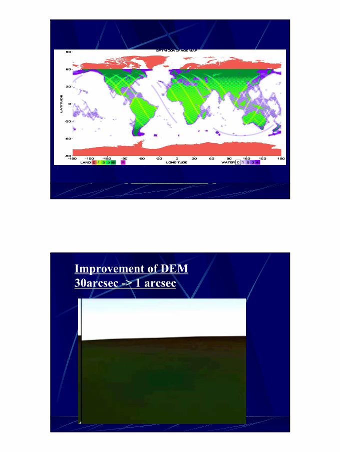
http://www-radar.jpl.nasa.gov/srtm/index.html
The Shuttle Radar Topography Mission (SRTM) is to map the world in three dimensions.
Using the Spaceborne Imaging Radar (SIR-C) and X-Band Synthetic Aperture Radar (X-SAR) hardware that flew twice on Space Shuttle Endeavour in 1994, SRTM will collect the following in a single 11-day shuttle flight:
41
42
43
Improvement of DEM30arcsec -> 1 arcsec
44
Next week LaboTo know what kind of application of RS are going on.To know what kind of researches are going on and why ?Application Review
5 Person / GroupSelect Application Topic
Rice Growth Monitoring in country XSlush and Burn Agriculture Monitoring in LaosFlood Monitoring in country XCarbon Fixation Estimation……
Search materials on Internet and LibraryCreate 5 pages ReportAvoid cut and paste, Citation
45
Next week LaboCreate 5 pages Report
IntroductionBackground: What is the problem, why important
Technical backgroundWhy RS can be applied to the topicWhat we can see from RS
Application ExamplesExisting Application Reviews if anyIf not, propose methodology
Technical ProblemsWhat is the problem ?Why it cannot be operational ?Cost, Frequency, Resolution, Accuracy ?What would be possible solutions ?