Volume title 1 The editors c 2007 Elsevier All rights reserved Chapter 1 Satisfiability solvers Carla P. Gomes, Henry Kautz, Ashish Sabharwal, and Bart Selman The past few years have seen an enormous progress in the performance of Boolean satisfia- bility (SAT) solvers. Despite the worst-case exponential run time of all known algorithms, satisfiability solvers are increasingly leaving their mark as a general-purpose tool in areas as diverse as software and hardware verification [28, 29, 30, 204], automatic test pattern generation [125, 197], planning [118, 177], scheduling [93], and even challenging prob- lems from algebra [214]. Annual SAT competitions have led to the development of dozens of clever implementations of such solvers [e.g. 12, 18, 65, 85, 99, 107, 137, 139, 148, 151, 155, 156, 158, 159, 167, 178, 189, 191, 212], an exploration of many new techniques [e.g. 14, 92, 136, 155, 159], and the creation of an extensive suite of real-world instances as well as challenging hand-crafted benchmark problems [cf. 104]. Modern SAT solvers provide a “black-box” procedure that can often solve hard structured problems with over a million variables and several million constraints. In essence, SAT solvers provide a generic combinatorial reasoning and search plat- form. The underlying representational formalism is propositional logic. However, the full potential of SAT solvers only becomes apparent when one considers their use in applica- tions that are not normally viewed as propositional reasoning tasks. For example, consider AI planning, which is a PSPACE-complete problem. By restricting oneself to polynomial size plans, one obtains an NP-complete reasoning problem, easily encoded as a Boolean satisfiability problem, which can be given to a SAT solver [117, 118]. In hardware and software verification, a similar strategy leads one to consider bounded model checking, where one places a bound on the length of possible error traces one is willing to con- sider [29]. Another example of a recent application SAT solvers is in computing stable models used in the answer set programming paradigm, a powerful knowledge representa- tion and reasoning approach [76]. In these applications – planning, verification, and answer set programming – the translation into a propositional representation (the “SAT encoding”) is done automatically and hidden from the user: the user only deals with the appropriate higher-level representation language of the application domain. Note that the translation
Carla P. Gomes, Henry Kautz,Ashish Sabharwal, and Bart Selman
The past few years have seen an enormous progress in the performance of Boolean satisfia-bility (SAT) solvers. Despite the worst-case exponential run time of all known algorithms,satisfiability solvers are increasingly leaving their markas a general-purpose tool in areasas diverse as software and hardware verification [28, 29, 30, 204], automatic test patterngeneration [125, 197], planning [118, 177], scheduling [93], and even challenging prob-lems from algebra [214]. Annual SAT competitions have led to the development of dozensof clever implementations of such solvers [e.g.12, 18, 65, 85, 99, 107, 137, 139, 148, 151,155, 156, 158, 159, 167, 178, 189, 191, 212], an exploration of many new techniques [e.g.14, 92, 136, 155, 159], and the creation of an extensive suite of real-world instances as wellas challenging hand-crafted benchmark problems [cf.104]. Modern SAT solvers providea “black-box” procedure that can often solve hard structured problems with over a millionvariables and several million constraints.
In essence, SAT solvers provide a generic combinatorial reasoning and search plat-form. The underlying representational formalism is propositional logic. However, the fullpotential of SAT solvers only becomes apparent when one considers their use in applica-tions that are not normally viewed as propositional reasoning tasks. For example, considerAI planning, which is a PSPACE-complete problem. By restricting oneself to polynomialsize plans, one obtains an NP-complete reasoning problem, easily encoded as a Booleansatisfiability problem, which can be given to a SAT solver [117, 118]. In hardware andsoftware verification, a similar strategy leads one to consider boundedmodel checking,where one places a bound on the length of possible error traces one is willing to con-sider [29]. Another example of a recent application SAT solvers is in computing stablemodels used in the answer set programming paradigm, a powerful knowledge representa-tion and reasoning approach [76]. In these applications – planning, verification, and answerset programming – the translation into a propositional representation (the “SAT encoding”)is done automatically and hidden from the user: the user onlydeals with the appropriatehigher-level representation language of the application domain. Note that the translation
2 1. Satisfiability solvers
to SAT generally leads to a substantial increase in problem representation. However, largeSAT encodings are no longer an obstacle for modern SAT solvers. In fact, for many combi-natorial search and reasoning tasks, the translation to SATfollowed by the use of a modernSAT solver is often more effective than a custom search engine running on the originalproblem formulation. The explanation for this phenomenon is that SAT solvers have beenengineered to such an extent that their performance is difficult to duplicate, even when onetackles the reasoning problem in its original representation.1
Although SAT solvers nowadays have found many applicationsoutside of knowledgerepresentation and reasoning, the original impetus for thedevelopment of such solvers canbe traced back to research in knowledge representation. In the early to mid eighties, thetradeoff between the computational complexity and the expressiveness of knowledge repre-sentation languages became a central topic of research. Much of this work originated witha seminal series of papers by Brachman and Levesque on complexity tradeoffs in knowl-edge representation, in general, and description logics, in particular [34, 35, 36, 132, 133].For a review of the state of the art of this work, see Chapter 3 of this handbook. A keyunderling assumption in the research on complexity tradeoffs for knowledge representa-tion languages is that the best way to proceed is to find the most elegant and expressiverepresentation language that still allows for worst-case polynomial time inference. In theearly nineties, this assumption was challenged in two earlypapers on SAT [154, 191]. Inthe first [154], the tradeoff between typical case complexity versus worst-case complexitywas explored. It was shown that most randomly generated SAT instances are actually sur-prisingly easy to solve (often in linear time), with the hardest instances only occurring ina rather small range of parameter settings of the random formula model. The second pa-per [191] showed that many satisfiable instances in the hardest region could still be solvedquite effectively with a new style of SAT solvers based on local search techniques. Theseresults challenged the relevance of the ”worst-case” complexity view of the world.2
The success of the current SAT solvers on many real world SAT instances with millionsof variables further confirms that typical case complexity and the complexity of real-worldinstances of NP-complete problems is much more amenable to effective general purposesolution techniques than worst-case complexity results might suggest. (For some initialinsights into why real-world SAT instances can often be solved efficiently, see [209].)Given these developments, it may be worthwhile to reconsider the study of complexitytradeoffs in knowledge representation languages by not insisting on worst-case polynomialtime reasoning but to allow for NP-complete reasoning sub-tasks that can be handled by aSAT solver. Such an approach would greatly extend the expressiveness of representationlanguages. The work on the use of SAT solvers to reason about stable models is a firstpromising example in this regard.
1 Each year the International Conference on Theory and Applications of Satisfiability Testing hosts a SATcompetition or race that highlights a new group of “world’s fastest” SAT solvers, and presents detailed per-formance results on a wide range of solvers [129, 130, 193, 128]. In the 2006 competition, over 30 solverscompeted on instances selected from thousands of benchmark problems. Most of these SAT solvers can bedownloaded freely from the web. For a good source of solvers,benchmarks, and other topics relevant toSAT research, we refer the reader to the websites SAT Live! (http://www.satlive.org) and SATLIB(http://www.satlib.org).
2 The contrast between typical- and worst-case complexity may appear rather obvious. However, note thatthe standard algorithmic approach in computer science is still largely based on avoiding any non-polynomialcomplexity, thereby implicitly acceding to a worst-case complexity view of the world. Approaches based on SATsolvers provide the first serious alternative.
In this chapter, we first discuss the main solution techniques used in modern SATsolvers, classifying them as complete and incomplete methods. We then discuss recent in-sights explaining the effectiveness of these techniques onpractical SAT encodings. Finally,we discuss several extensions of the SAT approach currentlyunder development. Theseextensions will further expand the range of applications toinclude multi-agent and proba-bilistic reasoning. For a review of the key research challenges for satisfiability solvers, werefer the reader to [116].
1.1 Definitions and Notation
A propositional or Boolean formula is a logic expressions defined over variables (or atoms)that take value in the setFALSE, TRUE, which we will identify with 0,1. A truthassignment(or assignment for short) to a setV of Boolean variables is a mapσ : V →0,1. A satisfying assignmentfor F is a truth assignmentσ such thatF evaluates to 1underσ . We will be interested in propositional formulas in a certain special form:F isin conjunctive normal form(CNF) if it is a conjunction (AND,∧) of clauses, where eachclause is a disjunction (OR,∨) of literals, and each literal is either a variable or its negation(NOT,¬). For example,F = (a∨¬b)∧ (¬a∨c∨d)∧ (b∨d) is a CNF formula with fourvariables and three clauses.
The Boolean Satisfiability Problem (SAT) is the following:Given a CNF formula F,does F have a satisfying assignment?This is the canonical NP-complete problem [45,134]. In practice, one is not only interested in this decision (“yes/no”) problem, but alsoin finding an actual satisfying assignment if there exists one. All practical satisfiabilityalgorithms, known as SAT solvers, do produce such an assignment if it exists.
It is natural to think of a CNF formula as a set of clauses and each clause as a set ofliterals. We use the symbolΛ to denote theempty clause, i.e., the clause that contains noliterals and is always unsatisfiable. A clause with only one literal is referred to as aunitclause. A clause with two literals is referred to as abinary clause. When every clauseof F hask literals, we refer toF as ak-CNF formula. The SAT problem restricted to2-CNF formulas is solvable in polynomial time, which for 3-CNF formulas, it is alreadyNP-complete. Apartial assignmentfor a formulaF is a truth assignment to a subset of thevariables ofF . For a partial assignmentρ for a CNF formulaF , F |ρ denotes thesimplifiedformula obtained by replacing the variables appearing inρ with their specified values,removing all clauses with at least oneTRUE literal, and deleting all occurrences ofFALSE
literals from the remaining clauses.CNF is the generally accepted norm for SAT solvers because ofits simplicity and
usefulness; indeed, many problems are naturally expressedas a conjunction of relativelysimple constraints. CNF also lends itself to theDPLL process to be described next. Theconstruction of Tseitin [201] can be used to efficiently convert any given propositionalformula to one in CNF form by adding new variables corresponding to its subformulas.For instance, given an arbitrary propositional formulaG, one would first locally re-writeeach of its logic operators in terms of∧,∨, and¬ to obtain, say,G = (((a∧ b)∨ (¬a∧¬b))∧¬c)∨d. To convert this to CNF, one possibility is to add four auxiliary variablesw,x,y, andz, construct clauses that encode the four relationsw↔ (a∧b), x↔ (¬a∧¬b),y↔ (w∨x), andz↔ (y∧¬c), and add to that the clause(z∨d).
s
4 1. Satisfiability solvers
1.2 SAT Solver Technology – Complete Methods
A completesolution method for the SAT problem is one that, given the input formulaF ,either produces a satisfying assignment forF or proves thatF is unsatisfiable. One ofthe most surprising aspects of the relatively recent practical progress of SAT solvers isthat the best complete methods remain variants of a process introduced several decadesago: theDPLL procedure, which performs a backtrack search in the space ofpartial truthassignments. The key feature ofDPLL is the efficient pruning of the search space basedon falsified clauses. Since its introduction in the early 1960’s, the main improvementsto DPLL have been smart branch selection heuristics, extensions like clause learning andrandomized restarts, and well-crafted data structures such as lazy implementations andwatched literals for fast unit propagation. This section isdevoted to understanding thesecomplete SAT solvers, also known assystematicsolvers.
1.2.1 The DPLL Procedure
The Davis-Putnam-Logemann-Loveland orDPLL procedure is a complete, systematicsearch process for finding a satisfying assignment for a given Boolean formula or prov-ing that it is unsatisfiable. Davis and Putnam [55] came up with the basic idea behind thisprocedure. However, it was only a couple of years later that Davis, Logemann, and Love-land [54] presented it in the efficient top-down form in which it is widely used today. It isessentially a branching procedure that prunes the search space based on falsified clauses.
Algorithm 1, DPLL-recursive(F,ρ), sketches the basicDPLL procedure on CNFformulas. The idea is to repeatedly select an unassigned literal ℓ in the input formulaFand recursively search for a satisfying assignment forF |ℓ andF¬ℓ. The step where suchanℓ is chosen is commonly referred to as thebranchingstep. Settingℓ to TRUE or FALSE
when making a recursive call is called adecision, and is associated with adecision levelwhich equals the recursion depth at that stage. The end of each recursive call, which takesF back to fewer assigned variables, is called thebacktrackingstep.
A partial assignmentρ is maintained during the search and output if the formula turnsout to be satisfiable. IfF |ρ contains the empty clause, the corresponding clause ofF fromwhich it came is said to beviolatedby ρ . To increase efficiency, unit clauses are immedi-ately set toTRUE as outlined in Algorithm1; this process is termedunit propagation. Pureliterals (those whose negation does not appear) are also set toTRUE as a preprocessing stepand, in some implementations, in the simplification processafter every branch.
Variants of this algorithm form the most widely used family of complete algorithms forformula satisfiability. They are frequently implemented inan iterative rather than recursivemanner, resulting in significantly reduced memory usage. The key difference in the itera-tive version is the extra step ofunassigningvariables when one backtracks. The naive wayof unassigning variables in a CNF formula is computationally expensive, requiring one toexamine every clause in which the unassigned variable appears. However, thewatchedliterals scheme provides an excellent way around this and will be described shortly.
1.2.2 Key Features of Modern DPLL-Based SAT Solvers
The efficiency of state-of-the-art SAT solvers relies heavily on various features that havebeen developed, analyzed, and tested over the last decade. These include fast unit propa-
Gomes et al. 5
Algorithm 1.1: DPLL-recursive(F,ρ)
Input : A CNF formulaF and an initially empty partial assignmentρOutput : UNSAT, or an assignment satisfyingFbegin
(F,ρ)← UnitPropagate(F,ρ)if F contains the empty clausethen return UNSATif F has no clauses leftthen
Outputρreturn SAT
ℓ← a literal not assigned byρ // the branching stepif DPLL-recursive(F|ℓ,ρ ∪ℓ) = SAT then return SATreturn DPLL-recursive(F|¬ℓ,ρ ∪¬ℓ)
end
subUnitPropagate(F)begin
while F contains no empty clause but has a unit clause xdoF ← F |xρ ← ρ ∪x
return (F,ρ)end
gation using watched literals, learning mechanisms, deterministic and randomized restartstrategies, effective constraint database management (clause deletion mechanisms), andsmart static and dynamic branching heuristics. We give a flavor of some of these below.
Variable (and value) selection heuristicis one of the features that vary the most fromone SAT solver to another. Also referred to as thedecision strategy, it can have a signif-icant impact on the efficiency of the solver (see e.g. [147] for a survey). The commonlyemployed strategies vary from randomly fixing literals to maximizing a moderately com-plex function of the current variable- and clause-state, such as the MOMS (MaximumOccurrence in clauses of Minimum Size) heuristic [110] or the BOHM heuristic [cf.31].One could select and fix the literal occurring most frequently in the yet unsatisfied clauses(the DLIS (Dynamic Largest Individual Sum) heuristic [148]), or choose a literal basedon its weight which periodically decays but is boosted if a clause in which it appears isused in deriving a conflict, like in the VSIDS (Variable StateIndependent Decaying Sum)heuristic [155]. Newer solvers likeBerkMin [85], Jerusat [156], MiniSat [65], andRSat [167] employ further variations on this theme.
Clause learning has played a critical role in the success of modern complete SATsolvers. The idea here is to cache “causes of conflict” in a succinct manner (as learnedclauses) and utilize this information to prune the search ina different part of the searchspace encountered later. We leave the details to Section1.2.3, which will be devoted fullyto clause learning. We will also see how clause learning provably exponentially improvesupon the basicDPLL procedure.
The watched literals schemeof Moskewicz et al. [155], introduced in their solverzChaff, is now a standard method used by most SAT solvers for efficient constraint prop-agation. This technique falls in the category of lazy data structures introduced earlier byZhang [212] in the solverSato. The key idea behind the watched literals scheme, as the
6 1. Satisfiability solvers
name suggests, is to maintain and “watch” two special literals for each active (i.e., notyet satisfied) clause that are notFALSE under the current partial assignment; these liter-als could either be set toTRUE or as yet unassigned. Recall that empty clauses halt theDPLL process and unit clauses are immediately satisfied. Hence, one can always find suchwatched literals in all active clauses. Further, as long as aclause has two such literals, itcannot be involved in unit propagation. These literals are maintained as follows. Supposea literalℓ is set toFALSE. We preform two maintenance operations. First, for every clauseC that hadℓ as a watched literal, we examineC and find, if possible, another literal towatch (one which isTRUE or still unassigned). Second, for every previously active clauseC′ that has now become satisfied because of this assignment ofℓ to FALSE, we make¬ℓ awatched literal forC′. By performing this second step, positive literals are given priorityover unassigned literals for being the watched literals.
With this setup, one can test a clause for satisfiability by simply checking whether atleast one of its two watched literals isTRUE. Moreover, the relatively small amount of extrabook-keeping involved in maintaining watched literals is well paid off when one unassignsa literalℓ by backtracking – in fact, one needs to do absolutely nothing! The invariant aboutwatched literals is maintained as such, saving a substantial amount of computation thatwould have been done otherwise. This technique has played a critical role in the successof SAT solvers, in particular those involving clause learning. Even when large numbers ofvery long learned clauses are constantly added to the clausedatabase, this technique allowspropagation to be very efficient – the long added clauses are not even looked at unless oneassigns a value to one of the literals being watched and potentially causes unit propagation.
Conflict-directed backjumping, introduced by Stallman and Sussman [196], allowsa solver to backtrack directly to a decision leveld if variables at levelsd or lower are theonly ones involved in the conflicts in both branches at a pointother than the branch variableitself. In this case, it is safe to assume that there is no solution extending the current branchat decision leveld, and one may flip the corresponding variable at leveld or backtrackfurther as appropriate. This process maintains the completeness of the procedure whilesignificantly enhancing the efficiency in practice.
Fast backjumping is a slightly different technique, relevant mostly to the now-popularFirstUIP learning scheme used in SAT solversGrasp [148] and zChaff [155]. It letsa solver to jump directly to a lower decision leveld when even one branch leads to aconflict involving variables at levelsd or lower only (in addition to the variable at thecurrent branch). Of course, for completeness, the current branch at leveld is not markedas unsatisfiable; one simply selects a new variable and valuefor level d and continueswith a new conflict clause added to the database and potentially a new implied variable.This is experimentally observed to increase efficiency in many benchmark problems. Note,however, that while conflict-directed backjumping is always beneficial, fast backjumpingmay not be so. It discards intermediate decisions which may actually be relevant and in theworst case will be made again unchanged after fast backjumping.
Assignment stack shrinkingbased on conflict clauses is a relatively new techniqueintroduced by Nadel [156] in their solverJerusat, and is now used in other solvers aswell. When a conflict occurs because a clauseC′ is violated and the resulting conflict clauseC to be learned exceeds a certain threshold length, the solverbacktracks to almost thehighest decision level of the literals inC. It then starts assigning toFALSE the unassignedliterals of the violated clauseC′ until a new conflict is encountered, which is expected toresult in a smaller and more pertinent conflict clause to be learned.
Gomes et al. 7
Conflict Clause Minimization was introduced by Een and Sorensson [65] in theirsolverMiniSat. The idea is to try to reduce the size of a learned conflict clauseC byrepeatedly identifying and removing any literals ofC that are implied to beFALSE when therest of the literals inC are set toFALSE. This is achieved using the subsumption resolutionrule, which lets one derive a clauseA from (x∨A) and(¬x∨B) whereB⊆ A (the derivedclauseA subsumes the antecedent(x∨A)). This rule can be generalized, at the expenseof extra computational cost that usually pays off, to a sequence of subsumption resolutionderivations such that the final derived clause subsumes the first antecedent clause.
Randomized restarts, introduced by Gomes et al. [92] and further developed by Bap-tista and Marques-Silva [15], allow clause learning algorithms to arbitrarily stop thesearchand restart their branching process from decision level zero. All clauses learned so far areretained and now treated as additional initial clauses. Most of the current SAT solvers,starting withzChaff [155], employ very aggressive restart strategies, sometimes restart-ing after as few as 20 to 50 backtracks. This has been shown to help immensely in reducingthe solution time. Theoretically, unlimited restarts, performed at the correct step, can prov-ably make clause learning very powerful. We will discuss randomized restarts in moredetails later in the chapter.
1.2.3 Clause Learning and Iterative DPLL
Algorithm 1.2gives the top-level structure of aDPLL-based SAT solver employing clauselearning. Note that this algorithm is presented here in theiterative format (rather thanrecursive) in which it is most widely used in today’s SAT solvers.
Algorithm 1.2: DPLL-ClauseLearning-IterativeInput : A CNF formulaOutput : UNSAT, or SAT along with a satisfying assignmentbegin
else ifstatus = SATthenOutput current assignment stackreturn SAT
else break
end
The procedureDecideNextBranch chooses the next variable to branch on (and thetruth value to set it to) using either a static or a dynamic variable selection heuristic. TheprocedureDeduce applies unit propagation, keeping track of any clauses thatmay becomeempty, causing what is known as a conflict. If all clauses havebeen satisfied, it declares
8 1. Satisfiability solvers
the formula to be satisfiable.3 The procedureAnalyzeConflict looks at the structureof implications and computes from it a “conflict clause” to learn. It also computes andreturns the decision level that one needs to backtrack. Notethat there is no explicit variableflip in the entire algorithm; one simply learns a conflict clause before backtracking, andthis conflict clause often implicitly “flips” the value of a decision or implied variable byunit propagation. This will become clearer when we discuss the details of conflict clauselearning and unique implication point.
In terms of notation, variables assigned values through theactual variable selectionprocess (DecideNextBranch) are calleddecisionvariables and those assigned values asa result of unit propagation (Deduce) are calledimplied variables.Decisionand impliedliterals are analogously defined. Upon backtracking, the last decision variable no longerremains a decision variable and might instead become an implied variable depending onthe clauses learned so far. Thedecision level of a decision variable xis one more than thenumber of current decision variables at the time of branching onx. Thedecision level of animplied variable yis the maximum of the decision levels of decision variables used to implyy; if y is implied a value without using any decision variable at all, y has decision level zero.The decision levelat any step of the underlyingDPLL procedure is the maximum of thedecision levels of all current decision variables, and zeroif there is no decision variableyet. Thus, for instance, if the clause learning algorithm starts off by branching onx, thedecision level ofx is 1 and the algorithm at this stage is at decision level 1.
A clause learning algorithm stops and declares the given formula to be unsatisfiablewhenever unit propagation leads to a conflict at decision level zero, i.e., when no variableis currently branched upon. This condition is sometimes referred to as aconflict at decisionlevel zero.
Clause learning grew out of work in artificial intelligence seeking to improve the per-formance of backtrack search algorithms by generating explanations for failure (backtrack)points, and then adding the explanations as new constraintson the original problem. Theresults of Stallman and Sussman [196], Genesereth [77], Davis [56], Dechter [58], de Kleerand Williams [57], and others proved this approach to be quite promising. Forgeneral con-straint satisfaction problems the explanations are called“conflicts” or “no-goods”; in thecase of Boolean CNF satisfiability, the technique becomes clause learning – the reasonfor failure is learned in the form of a “conflict clause” whichis added to the set of givenclauses. Despite the initial success, the early work in thisarea was limited by the large num-bers of no-goods generated during the search, which generally involved many variables andtended to slow the constraint solvers down. Clause learningowes a lot of its practical suc-cess to subsequent research exploiting efficient lazy data structures and constraint databasemanagement strategies. Through a series of papers and oftenaccompanying solvers, Frostand Dechter [74], Bayardo Jr. and Miranker [16], Marques-Silva and Sakallah [148], Ba-yardo Jr. and Schrag [18], Zhang [212], Moskewicz et al. [155], Zhang et al. [216], andothers showed that clause learning can be efficiently implemented and used to solve hardproblems that cannot be approached by any other technique.
In general, the learning process hidden inAnalyzeConflict is expected to save usfrom redoing the same computation when we later have an assignment that causes conflict
3 In some implementations involving lazy data structures, solvers do not keep track of the actual number ofsatisfied clauses. Instead, the formula is declared to be satisfiable when all variables have been assigned a truthvalue and no conflict is created by this assignment.
Gomes et al. 9
due in part to the same reason. Variations of such conflict-driven learning include differentways of choosing the clause to learn (differentlearning schemes) and possibly allowingmultiple clauses to be learned from a single conflict. We nextdiscuss formalize the graph-based framework used to define and compute conflict clauses.
Implication Graph and Conflicts
Unit propagation can be naturally associated with animplication graphthat captures allpossible ways of deriving all implied literals from decision literals. In what follows, weuse the termknown clausesto refer to the clauses of the input formula as well as to allclauses that have been learned by the clause learning process so far.
Definition 1. Theimplication graph Gat a given stage ofDPLL is a directed acyclic graphwith edges labeled with sets of clauses. It is constructed asfollows:
Step 1: Create a node for each decision literal, labeled withthat literal. These will bethe indegree zero source nodes ofG.
Step 2: While there exists a known clauseC = (l1∨ . . . lk∨ l) such that¬l1, . . . ,¬lklabel nodes inG,
i. Add a node labeledl if not already present inG.
ii. Add edges(l i , l),1≤ i ≤ k, if not already present.
iii. Add C to the label set of these edges. These edges are thought of asgrouped together and associated with clauseC.
Step 3: Add toG a special “conflict” nodeΛ. For any variablex that occurs bothpositively and negatively inG, add directed edges fromx and¬x to Λ.
Since all node labels inG are distinct, we identify nodes with the literals labeling them.Any variablex occurring both positively and negatively inG is aconflict variable, andx aswell as¬x areconflict literals. G contains aconflict if it has at least one conflict variable.DPLL at a given stage has aconflictif the implication graph at that stage contains a conflict.A conflict can equivalently be thought of as occurring when the residual formula containsthe empty clauseΛ.
By definition, an implication graph may not contain a conflictat all, or it may containmany conflict variables and several ways of deriving any single literal. To better understandand analyze a conflict when it occurs, we work with a subgraph of an implication graph,called theconflict graph(see Figure1.1), that captures only one among possibly manyways of reaching a conflict from the decision variables usingunit propagation.
Definition 2. A conflict graph His any subgraph of an implication graph with the follow-ing properties:
(a) H containsΛ and exactly one conflict variable.
(b) All nodes inH have a path toΛ.
(c) Every nodel in H other thanΛ either corresponds to a decision literal or hasprecisely the nodes¬l1,¬l2, . . . ,¬lk as predecessors where(l1∨ l2∨ . . .∨ lk∨ l) isa known clause.
10 1. Satisfiability solvers
a cut corresponding
to clause (¬ a ∨ ¬ b)
¬ p
¬ q
b
a
¬ t
¬ x1
¬ x2
¬ x3
y
¬¬¬¬ y
Λ
reason side conflict side
conflict
variable
Figure 1.1: A conflict graph
While an implication graph may or may not contain conflicts, a conflict graph alwayscontains exactly one. The choice of the conflict graph is partof the strategy of the solver.A typical strategy will maintain one subgraph of an implication graph that has properties(b) and (c) from Definition2, but not property (a). This can be thought of as aunique infer-encesubgraph of the implication graph. When a conflict is reached,this unique inferencesubgraph is extended to satisfy property (a) as well, resulting in a conflict graph, which isthen used to analyze the conflict.
Conflict clauses
For a subsetU of the vertices of a graph, theedge-cut(henceforth called a cut) correspond-ing toU is the set of all edges going from vertices inU to vertices not inU .
Consider the implication graph at a stage where there is a conflict and fix a conflictgraph contained in that implication graph. Choose any cut inthe conflict graph that has alldecision variables on one side, called thereason side, andΛ as well as at least one conflictliteral on the other side, called theconflict side. All nodes on the reason side that have atleast one edge going to the conflict side form acauseof the conflict. The negations of thecorresponding literals forms theconflict clauseassociated with this cut.
Learning Schemes
The essence of clause learning is captured by thelearning schemeused to analyze andlearn the “cause” of a failure. More concretely, different cuts in a conflict graph separatingdecision variables from a set of nodes containingΛ and a conflict literal correspond todifferent learning schemes (see Figure1.2). One may also define learning schemes basedon cuts not involving conflict literals at all such as a schemesuggested by Zhang et al.[216], but the effectiveness of such schemes is not clear. These will not be consideredhere.
It is insightful to think of thenondeterministicscheme as the most general learningscheme. Here we select the cut nondeterministically, choosing, whenever possible, onewhose associated clause is not already known. Since we can repeatedly branch on the
Gomes et al. 11
FirstNewCut clause
(x1 ∨ x2 ∨ x3)
Decision clause
(p ∨ q ∨ ¬ b)
1UIP clause
t
rel-sat clause
(¬ a ∨ ¬ b)
¬ p
¬ q
b
a
¬ t
¬ x1
¬ x2
¬ x3
y
¬¬¬¬ y
Λ
Figure 1.2: Learning schemes corresponding to different cuts in the conflict graph
same last variable, nondeterministic learning subsumes learning multiple clauses from asingle conflict as long as the sets of nodes on the reason side of the corresponding cutsform a (set-wise) decreasing sequence. For simplicity, we will assume that only one clauseis learned from any conflict.
In practice, however, we employ deterministic schemes. Thedecisionscheme [216],for example, uses the cut whose reason side comprises all decision variables.relsat [18]uses the cut whose conflict side consists of all implied variables at the current decisionlevel. This scheme allows the conflict clause to have exactlyone variable from the currentdecision level, causing an automatic flip in its assignment upon backtracking. In the ex-ample depicted in Figure1.2, the decision clause(p∨q∨¬b) hasb as the only variablefrom the current decision level. After learning this conflict clause and backtracking byunassigningb, the truth values ofp andq (both FALSE) immediately imply¬b, flippingthe value ofb from TRUE to FALSE.
This nice flipping property holds in general for allunique implication points(UIPs)[148]. A UIP of an implication graph is a node at the current decision leveld such that anypath from the decision variable at leveld to the conflict variable as well as its negation mustgo through it. Intuitively, it is asinglereason at leveld that causes the conflict. Whereasrelsat uses the decision variable as the obvious UIP,Grasp [148] and zChaff [155]useFirstUIP, the one that is “closest” to the conflict variable.Grasp also learns multipleclauses when faced with a conflict. This makes it typically require fewer branching stepsbut possibly slower because of the time lost in learning and unit propagation.
The concept of UIP can be generalized to decision levels other than the current one.The1UIP schemecorresponds to learning the FirstUIP clause of the current decision level,the 2UIP schemeto learning the FirstUIP clauses of both the current level and the onebefore, and so on. Zhang et al. [216] present a comparison of all these and other learningschemes and conclude that 1UIP is quite robust and outperforms all other schemes theyconsider on most of the benchmarks.
Another learning scheme, which underlies the proof of a theorem to be presented inthe next section, is theFirstNewCutscheme [21]. This scheme starts with the cut that isclosest to the conflict literals and iteratively moves it back toward the decision variablesuntil a conflict clause that is not already known is found; hence the name FirstNewCut.
12 1. Satisfiability solvers
1.2.4 A Proof Complexity Perspective
Propositional proof complexity is the study of the structure of proofs of validity of mathe-matical statements expressed in a propositional or Booleanform. Cook and Reckhow [46]introduced the formal notion of a proof system in order to study mathematical proofs froma computational perspective. They defined a propositional proof system to be an efficientalgorithmA that takes as input a propositional statementSand a purported proofπ of itsvalidity in a certain pre-specified format. The crucial property of A is that for all invalidstatementsS, it rejects the pair(S,π) for all π, and for all valid statementsS, it acceptsthe pair(S,π) for some proofπ. This notion of proof systems can be alternatively formu-lated in terms of unsatisfiable formulas — those that areFALSE for all assignments to thevariables.
They further observed that if there is no propositional proof system that admits short(polynomial in size) proofs of validity of all tautologies,i.e., if there exist computation-ally hard tautologies for every propositional proof system, then the complexity classes NPand co-NP are different, and hence P6= NP. This observation makes finding tautologicalformulas (equivalently, unsatisfiable formulas) that are computationally difficult for vari-ous proof systems one of the central tasks of proof complexity research, with far reachingconsequences to complexity theory and Computer Science in general. These hard formu-las naturally yield a hierarchy of proof systems based on thesizes of proofs they admit.Tremendous amount of research has gone into understanding this hierarchical structure.Beame and Pitassi [22] summarize many of the results obtained in this area.
To understand current complete SAT solvers, we focus on the proof system calledresolution, denoted henceforth asRES. It is a very simple system with only one rulewhich applies to disjunctions of propositional variables and their negations:(a OR b) and((NOT a) OR c) together imply(b OR c). Repeated application of this rule suffices to de-rive an empty disjunction if and only if the initial formula is unsatisfiable; such a derivationserves as a proof of unsatisfiability of the formula.
Despite its simplicity, unrestricted resolution as definedabove (also calledgeneral res-olution) is hard to implement efficiently due to the difficulty of finding good choices ofclauses to resolve; natural choices typically yield huge storage requirements. Various re-strictions on the structure of resolution proofs lead to less powerful but easier to implementrefinements that have been studied extensively in proof complexity. Those of special in-terest to us aretree-like resolution, where every derived clause is used at most once in therefutation, andregular resolution, where every variable is resolved upon at most one in any“path” from the initial clauses to the empty clause. While these and other refinements aresound and complete as proof systems, they differ vastly in efficiency. For instance, in a se-ries of results, Bonet et al. [32], Bonet and Galesi [33], and Buresh-Oppenheim and Pitassi[39] have shown that regular, ordered, linear, positive, negative, and semantic resolutionare all exponentially stronger than tree-like resolution.On the other hand, Bonet et al. [32]and Alekhnovich et al. [6] have proved that tree-like, regular, and ordered resolution areexponentially weaker thanRES.
Most of today’s complete SAT solvers implement a subset of the resolution proof sys-tem. However, till recently, it wasn’t clear where exactly do they fit in the proof systemhierarchy and how do they compare to refinements of resolution such as regular resolution.Clause learning and random restarts can be considered to be two of the most importantideas that have lifted the scope of modern SAT solvers from experimental toy problems
Gomes et al. 13
to large instances taken from real world challenges. Despite overwhelming empirical ev-idence, for many years not much was known of the ultimate strengths and weaknesses ofthe two.
Beame, Kautz, and Sabharwal [21, 179] answered several of these questions in a for-mal proof complexity framework. They gave the first precise characterization of clauselearning as a proof system calledCL and began the task of understanding its power byrelating it to resolution. In particular, they showed that with a new learning scheme calledFirstNewCut, clause learning can provide exponentially shorter proofs than any proper re-finement of general resolution satisfying a natural self-reduction property. These includeregular and ordered resolution, which are already known to be much stronger than the or-dinary DPLL procedure which captures most of the SAT solvers that do not incorporateclause learning. They also showed that a slight variant of clause learning with unlimitedrestarts is as powerful as general resolution itself.
From the basic proof complexity point of view, only familiesof unsatisfiable formulasare of interest because only proofs of unsatisfiability can be large; minimum proofs ofsatisfiability are linear in the number of variables of the formula. In practice, however,many interesting formulas are satisfiable. To justify the approach of using a proof systemCL, we refer to the work of Achlioptas, Beame, and Molloy [2] who have shown hownegative proof complexity results for unsatisfiable formulas can be used to derive timelower bounds for specific inference algorithms, especiallyDPLL, running on satisfiableformulas as well. The key observation in their work is that before hitting a satisfyingassignment, an algorithm is very likely to explore a large unsatisfiable part of the searchspace that corresponds to the first bad variable assignment.
Proof complexity does not capture everything we intuitively mean by the power of areasoning system because it says nothing about how difficultit is to find shortest proofs.However, it is a good notion with which to begin our analysis because the size of proofsprovides a lower bound on the running time of any implementation of the system. In thesystems we consider, a branching function, which determines which variable to split uponor which pair of clauses to resolve, guides the search. A negative proof complexity resultfor a system (“proofs must be large in this system”) tells us that a family of formulas isintractable even with a perfect branching function; likewise, a positive result (“small proofsexist”) gives us hope of finding a good branching function, i.e., a branching function thathelps us uncover a small proof.
We begin with an easy to prove relationship betweenDPLL (without clause learning)and tree-like resolution (for a formal proof, see e.g. [179]).
Proposition 1. For a CNF formula F, the size of the smallestDPLL refutation of F is equalto the size of the smallest tree-like resolution refutationof F.
The interesting part is to understand what happens when clause learning is brought intothe picture. It has been previously observed by Lynce and Marques-Silva [144] that clauselearning can be viewed as adding resolvents to a tree-like resolution proof. The followingresults show further that clause learning, viewed as a propositional proof systemCL, isexponentially stronger than tree-like resolution. This explains, formally, the performancegains observed empirically when clause learning is added toDPLL based solvers.
14 1. Satisfiability solvers
Clause Learning Proofs
The notion of clause learning proofs connects clause learning with resolution and providesthe basis for the complexity bounds to follow. If a given formula F is unsatisfiable, theclause learning basedDPLL process terminates with a conflict at decision level zero. Sinceall clauses used in this final conflict themselves follow directly or indirectly fromF , thisfailure of clause learning in finding a satisfying assignment constitutes a logical proof ofunsatisfiability ofF . In an informal sense, we denote byCL the proof system consisting ofall such proofs; this can be made precise using the notion of abranching sequence [21]. Theresults below compare the sizes of proofs inCL with the sizes of (possibly restricted) reso-lution proofs. Note that clause learning algorithms can useone of many learning schemes,resulting in different proofs.
We next define what it means for a refinement of a proof system tobe natural andproper. LetCS(F) denote the length of the short refutation of a formulaF under a proofsystemS.
Definition 3 ([21, 179]). For proof systemsSandT, and a functionf : N→ [1,∞),
• Sis natural if for any formulaF and restrictionρ on its variables,CS(F|ρ)≤CS(F).
• S is arefinementof T if proofs inSare also (restricted) proofs inT.
• S is f (n)-proper as a refinement ofT if there exists a witnessing familyFn offormulas such thatCS(Fn) ≥ f (n) ·CT(Fn). The refinement isexponentially-proper
if f (n) = 2nΩ(1)andsuper-polynomially-properif f (n) = nω(1).
Under this definition, tree-like, regular, linear, positive, negative, semantic, and or-dered resolution are natural refinements ofRES, and further, tree-like, regular, and orderedresolution are exponentially-proper [32, 6].
Now we are ready to state the somewhat technical theorem relating the clause learningprocess to resolution, whose corollaries are nonetheless easy to understand. The proofof this theorem is based on an explicit construction of so-called “proof-trace extension”formulas, which interestingly allow one to translateanyknown separation result betweenRES and a natural proper refinementSof RES into a separation betweenCL andS.
Theorem 1([21, 179]). For any f(n)-proper natural refinement S ofRES and forCL usingthe FirstNewCut scheme and no restarts, there exist formulas Fn such thatCS(Fn) ≥f (n) ·CCL(Fn).
Corollary 1. CL can provide exponentially shorter proofs than tree-like, regular, and or-dered resolution.
Corollary 2. EitherCL is not a natural proof system or it is equivalent in strength to RES.
We remark that this leaves open the possibility thatCL may not be able to simulateall regular resolution proofs. In this context, MacKenzie [145] has used arguments similarto those of Beame et al. [19] to prove that a natural variant of clause learning can indeedsimulate all of regular resolution.
Finally, let CL-- denote the variant ofCL where one is allowed to branch on a literalwhose value is already set explicitly or because of unit propagation. Of course, such a
Gomes et al. 15
relaxation is useless in ordinaryDPLL; there is no benefit in branching on a variable thatdoesn’t even appear in the residual formula. However, with clause learning, such a branchcan lead to an immediate conflict and allow one to learn a key conflict clause that wouldotherwise have not been learned. This property can be used toprove thatRES can beefficiently simulated byCL-- with enough restarts. In this context, a clause learning schemewill be callednon-redundantif on a conflict, it always learns a clause not already known.Most of the practical clause learning schemes are non-redundant.
Theorem 2 ([21, 179]). CL-- with any non-redundant scheme and unlimited restarts ispolynomially equivalent toRES.
We note that by choosing the restart points in a smart way,CL together with restartscan be converted into acompletealgorithm for satisfiability testing, i.e., for all unsatisfiableformulas given as input, it will halt and provide a proof of unsatisfiability [15, 92]. Thetheorem above makes a much stronger claim about a slight variant of CL, namely, withenough restarts, this variant can always find proofs of unsatisfiability that are as short asthose ofRES.
1.2.5 Symmetry Breaking
One aspect of many theoretical as well as real-world problems that merits attention is thepresence ofsymmetryor equivalenceamongst the underlying objects. Symmetry can bedefined informally as a mapping of a constraint satisfactionproblem (CSP) onto itself thatpreserves its structure as well as its solutions. The concept of symmetry in the context ofSAT solvers and in terms of higher level problem objects is best explained through someexamples of the many application areas where it naturally occurs. For instance, in FPGA(field programmable gate array) routing used in electronicsdesign, all available wires orchannels used for connecting two switch boxes are equivalent; in our design, it does notmatter whether we use wire #1 between connector X and connector Y, or wire #2, orwire #3, or any other available wire. Similarly, in circuit modeling, all gates of the same“type” are interchangeable, and so are the inputs to a multiple fanin AND or OR gate (i.e.,a gate with several inputs); in planning, all identical boxes that need to be moved fromcity A to city B are equivalent; in multi-processor scheduling, all available processors areequivalent; in cache coherency protocols in distributed computing, all available identicalcaches are equivalent. A key property of such objects is thatwhen selectingk of them, wecan choose,without loss of generality, anyk. This without-loss-of-generality reasoning iswhat we would like to incorporate in an automatic fashion.
The question of symmetry exploitation that we are interested in addressing arises wheninstances from domains such as the ones mentioned above are translated into CNF formulasto be fed to a SAT solver. A CNF formula consists of constraints over different kinds ofvariables that typically represent tuples of these high level objects (e.g. wires, boxes, etc.)and their interaction with each other. For example, during the problem modeling phase,we could have a Boolean variablezw,c that isTRUE iff the first end of wirew is attachedto connectorc. When this formula is converted into DIMACS format for a SAT solver,thesemantic meaningof the variables, that, say, variable 1324 is associated with wire #23and connector #5, is discarded. Consequently, in this translation, the global notion of theobvious interchangeability of the set of wire objects is lost, and instead manifests itselfindirectly as a symmetry between the (numbered) variables of the formula and therefore
16 1. Satisfiability solvers
also as a symmetry within the set of satisfying (or un-satisfying) variable assignments.These sets of symmetric satisfying and un-satisfying assignments artificially explode boththe satisfiable and the unsatisfiable parts of the search space, the latter of which can be achallenging obstacle for a SAT solver searching for a satisfying assignment.
One of the most successful techniques for handling symmetryin both SAT and generalCSPs originates from the work of Puget [169], who showed that symmetries can bebro-kenby adding one lexicographic ordering constraint per symmetry. Crawford et al. [49]showed how this can be done adding a set of simple “lex-constraints” orsymmetry breakingpredicates(SBPs) to the input specification to weed out all but the lexically-first solutions.The idea is to identify the group of permutations of variables that keep the CNF formulaunchanged. For each such permutationπ, clauses are added so that for every satisfyingassignmentσ for the original problem, whose permutationπ(σ) is also a satisfying as-signment, only the lexically-first ofσ andπ(σ) satisfies the added clauses. In the contextof CSPs, there has been a lot of work in the area of SBPs. Petrieand Smith [165] extendedthe idea to value symmetries, Puget [171] applied it to products of variable and value sym-metries, and Walsh [207] generalized the concept to symmetries acting simultaneously onvariables and values, on set variables, etc. Puget [170] has recently proposed a techniquefor creating dynamic lex-constraints, with the goal of minimizing adverse interaction withthe variable ordering used in the search tree.
In the context of SAT, value symmetries for the high-level variables naturally manifestthemselves as low-level variable symmetries, and work on SBPs has taken a different path.Tools such asShatter by Aloul et al. [7] improve upon the basic SBP technique by usinglex-constraints whose size is only linear in the number of variables rather than quadratic.Further, they use graph isomorphism detectors likeSaucy by Darga et al. [50] to generatesymmetry breaking predicates only for the generators of thealgebraic groups of symme-try. This latter problem of computing graph isomorphism, however, is not known to haveany polynomial time algorithms, and is conjectured to be strictly between the complexityclasses P and NP [cf.124]. Hence, one must resort to heuristic or approximate solutions.Further, while there are formulas for which few SBPs suffice,the number of SBPs oneneeds to add in order to breakall symmetries can be exponential. This is typically handledin practice by discarding “large” symmetries, i.e., those involving too many variables withrespect to a fixed threshold. This may, however, sometimes result in a much slower SATsolutions in domains such as clique coloring and logistics.
A very different and indirect approach for addressing symmetry is embodied in SATsolvers such asPBS by Aloul et al. [8], pbChaff by Dixon et al. [62], andGalena byChai and Kuehlmann [41], which utilize non-CNF formulations known as pseudo-Booleaninequalities. Their logic reasoning are based on what is called the Cutting Planes proofsystem which, as shown by Cook et al. [47], is strictly stronger than resolution on whichDPLL type CNF solvers are based. Since this more powerful proof system is difficult toimplement in its full generality, pseudo-Boolean solvers often implement only a subset ofit, typically learning only CNF clauses or restricted pseudo-Boolean constraints upon aconflict. Pseudo-Boolean solvers may lead to purely syntactic representational efficiencyin cases where a single constraint such asy1 +y2 + . . .+yk ≤ 1 is equivalent to
(k2
)
binaryclauses. More importantly, they are relevant to symmetry because they sometimes allowimplicit encoding. For instance, the single constraintx1+x2+ . . .+xn≤movern variablescaptures the essence of the pigeonhole formulaPHPn
m overnmvariables which is provablyexponentially hard to solve using resolution-based methods without symmetry consider-
Gomes et al. 17
ations. This implicit representation, however, is not suitable in certain applications suchas clique coloring and planning that we discuss. In fact, forunsatisfiable clique coloringinstances, even pseudo-Boolean solvers provably require exponential time.
One could conceivably keep the CNF input unchanged but modify the solver to detectand handle symmetries during the search phase as they occur.Although this approach isquite natural, we are unaware of its implementation in a general purpose SAT solver besidessEqSatz by Li et al. [138], which has been shown to be effective on matrix multiplicationand polynomial multiplication problems. Symmetry handling during search has been ex-plored with mixed results in the CSP domain using frameworkslike SBDD and SBDS [e.g.66, 67, 79, 82]. Related work in SAT has been done in the specific areas of automatic testpattern generation by Marques-Silva and Sakallah [149] and SAT-based model checking byShtrichman [192]. In both cases, the solver utilizes global information obtained at a stageto make subsequent stages faster. In other domain-specific work on symmetries in prob-lems relevant to SAT, Fox and Long [68] propose a framework for handling symmetry inplanning problems solved using the planning graph framework. They detect equivalencebetween various objects in the planning instance and use this information to reduce thesearch space explored by their planner. Unlike typical SAT-based planners, this approachdoes not guarantee plans of optimal length when multiple (non-conflicting) actions are al-lowed to be performed at each time step in parallel. Fortunately, this issue does not arisein theSymChaff approach for SAT to be mentioned shortly.
Dixon et al. [61] give a generic method of representing and dynamically maintainingsymmetry in SAT solvers using algebraic techniques that guarantee polynomial size un-satisfiability proofs of many difficult formulas. The strength of their work lies in a stronggroup theoretic foundation and comprehensiveness in handling all possible symmetries.The computations involving group operations that underlietheir current implementationare, however, often quite expensive.
When viewing complete SAT solvers as implementations of proof systems, the chal-lenge with respect to symmetry exploitation is to push the underlying proof system up inthe weak-to-strong proof complexity hierarchy without incurring the significant cost thattypically comes from large search spaces associated with complex proof systems. Whilemost of the current SAT solvers implement subsets of the resolution proof system, a differ-ent kind of solver calledSymChaff [179, 180] brings it up closer tosymmetric resolution,a proof system known to be exponentially stronger than resolution [202, 126]. More criti-cally, it achieves this in a time- and space-efficient manner. Interestingly, whileSymChaffinvolves adding structure to the problem description, it still stays within the realm of SATsolvers (as opposed to using a constraint programming (CP) approach), thereby exploitingthe many benefits of the CNF form and the advances in state-of-the-art SAT solvers.
As a structure-aware solver,SymChaff incorporates several new ideas, including sim-ple but effective symmetry representation, multiway branching based on variable classesand symmetry sets, and symmetric learning as an extension ofclause learning to multi-way branches. Two key places where it differs from earlier approaches are in using highlevel problem description to obtain symmetry information (instead of trying to recover itfrom the CNF formula) and in maintaining this information dynamically but without us-ing a complex group theoretic machinery. This allows it to overcome many drawbacksof previously proposed solutions. It is shown, in particular, that straightforward annota-tion in the usual PDDL specification of planning problems is enough to automatically andquickly generate relevant symmetry information, which in turn makes the search for an op-
18 1. Satisfiability solvers
timal plan several orders of magnitude faster. Similar performance gains are seen in otherdomains as well.
1.3 SAT Solver Technology – Incomplete Methods
An incompletemethod for solving the SAT problem is one that does not provide the guar-antee that it will eventually either report a satisfying assignment or prove the given formulaunsatisfiable. Such a method is typically run with a pre-set limit, after which it may or maynot produce a solution. Unlike the systematic solvers basedon an exhaustive branchingand backtracking search, incomplete methods are based onstochastic local searchor SLS.On many classes of problems, such incomplete methods for SATsignificantly outperformDPLL-based methods. Since the early 1990’s, there has been a tremendous amount ofresearch on designing, understanding, and improving localsearch methods for SAT [e.g.71, 94, 95, 99, 102, 103, 105, 139, 166, 186] as well as on hybrid approaches that attemptto combine DPLL and local search methods [e.g.9, 96, 150, 175]. We begin this section bydiscussing two methods that played a key role in the success of local search in SAT, namelyGSAT [191] andWalksat [189]. We will then explore the phase transition phenomenon inrandom SAT and a relatively new local search technique called Survey Propagation. Wenote that there are also solution techniques based on the discrete Lagrangian [205, 211]and on the interior point method [113], which we will not discuss.
The original impetus for trying a local search method on satisfiability problems was thesuccessful application of such methods for finding solutions to largeN-queens problems,first using a connectionist system by Adorf and Johnston [5], and then using greedy localsearch by Minton et al. [153]. It was originally assumed that this success simply indicatedthatN-queens was aneasyproblem, and researchers felt that such techniques would fail inpractice for SAT. In particular, it was believed that local search methods would easily getstuck in local minima, with a few clauses remaining unsatisfied. TheGSAT experimentsshowed, however, that certain local search strategies often do reach global minima, in manycases much faster than any systematic search strategies.
GSAT is based on a randomized local search technique [140, 162]. The basicGSATprocedure, described as Algorithm1.3, starts with a randomly generated truth assignment.It then greedily changes (‘flips’) the assignment of the variable that leads to the greatestdecrease in the total number of unsatisfied clauses. Such flips are repeated until eithera satisfying assignment is found or a pre-set maximum numberof flips (MAX -FLIPS) isreached. This process is repeated as needed, up to a maximum of MAX -TRIES times.
Selman et al. [191] showed thatGSAT substantially outperformed even the best back-tracking search procedures of the time on various classes offormulas, including randomlygenerated formulas and SAT encodings of graph coloring problems [112]. The search ofGSAT typically begins with a rapid greedy descent towards a better assignment, followedby a long sequences of “sideways” moves. Each sequence of sideways moves is referred toas aplateau. Experiments indicate that in practice,GSAT spends most of its time movingfrom plateau to plateau, which motivates studying various modifications in order to speedup this process [187, 188]. One of the most successful strategies is to introduce noise intothe search in the form of uphill moves, which forms the basis of the now well-known localsearch method for SAT calledWalksat [189].
Gomes et al. 19
Algorithm 1.3: GSAT (F)
Input : A CNF formulaFParameters : IntegersMAX -FLIPS, MAX -TRIES
Output : A satisfying assignment forF , or FAILbegin
for i← 1 to MAX -TRIES doσ ← a randomly generated truth assignment forFfor j ← 1 to MAX -FLIPS do
if σ satisfies Fthen return σ // successv← a variable flipping which results in the greatest decrease
(possibly negative) in the number of unsatisfied clausesFlip v in σ
return FAIL // no satisfying assignment found
end
Walksat interleaves the greedy moves ofGSAT with random walk moves of a standardMetropolis search. It further focuses the search by always selecting the variable to flip froman (randomly chosen) unsatisfied clauseC. If there is a variable inC flipping which doesnot turn any currently satisfied clauses to unsatisfied, it flips this variable (the “freebie”move). Otherwise, with a certain probability, it flips a random literal ofC (the “randomwalk” move), and with the remaining probability, it flips a variable inC that minimizesthebreak-count, i.e., the number of currently satisfied clauses that becomeunsatisfied (the“greedy” move).Walksat in presented in detail as Algorithm1.4. One of its parameters,in addition to the maximum number of tries and flips, is thenoise p∈ [0,1], which controlshow often are uphill moves considered during the stochasticsearch.
When one compares the biased random walk strategy ofWalksat on hard random 3-CNF formulas against basicGSAT, the simulated annealing process of Kirkpatrick et al.[120], and a pure random walk strategy, the biased random walk process significantly out-performs the other methods [188]. In the years following the development ofWalksat,many similar methods have been shown to be highly effective on not only random formu-las but on many classes of structured instances, such as encodings of circuit design prob-lems, Steiner tree problems, problems in finite algebra, andAI planning [cf.105]. Variousextensions of the basic process have also been explored, such as dynamic search poli-cies likeadapt-novelty [103], incorporating unit clause elimination as in the solverUnitWalk [99], and exploiting problem structure for increased efficiency [166]. Recently,it was shown that the performance of stochastic solvers on many structured problems canbe further enhanced by using new SAT encodings that are designed to be effective for localsearch [168].
1.3.1 The Phase Transition Phenomenon in Randomk-SAT
One of the key motivations in the early 1990’s for studying incomplete, stochastic meth-ods for solving SAT problems was the finding thatDPLL-based systematic solvers performquite poorly on certain randomly generated formulas. Consider a randomk-CNF formulaF onn variables generated by independently creatingmclauses as follows: for each clause,selectk distinct variables uniformly at random out of then variables and negate each vari-
20 1. Satisfiability solvers
Algorithm 1.4: Walksat (F)
Input : A CNF formulaFParameters : IntegersMAX -FLIPS, MAX -TRIES; noise parameterp∈ [0,1]Output : A satisfying assignment forF , or FAILbegin
for i← 1 to MAX -TRIES doσ ← a randomly generated truth assignment forFfor j ← 1 to MAX -FLIPS do
if σ satisfies Fthen return σ // successC← an unsatisfied clause ofF chosen at randomif ∃ variable x∈C with break-count = 0then
v← x // the freebie move
elseWith probability p: // the random walk move
v← a variable inC chosen at randomWith probability 1− p: // the greedy move
v← a variable inC with the smallest break-countFlip v in σ
return FAIL // no satisfying assignment found
end
able with probability 0.5. WhenF is chosen from this distribution, Mitchell, Selman, andLevesque [154] observed that the median hardness of the problems is very nicely character-ized by a key parameter: theclause-to-variable ratio, m/n, typically denoted byα. Theyobserved that problem hardness peaks in a critically constrained region determined byαalone. The left pane of Figure1.3 depicts the now well-known “easy-hard-easy” patternof SAT and other combinatorial problems, as the key parameter (in this caseα) is varied.For random 3-SAT, this region has been experimentally shownto be aroundα ≈ 4.26 (see[48, 121] for early results), and has provided challenging benchmarks as a test-bed for SATsolvers.
Figure 1.3: The phase transition phenomenon in random 3-SAT. Left: Computational hard-ness peaks atα ≈ 4.26. Right: Problems change from being mostly satisfiable to mostlyunsatisfiable. The transitions sharpen as the number of variables grows.
Gomes et al. 21
This critically constrained region marks a stark transition not only in the computationalhardness of random SAT instances but also in their satisfiability itself. The right pane ofFigure1.3 shows the fraction of random formulas that are unsatisfiable, as a function ofα. We see that nearly all problems withα below the critical region (the under-constrainedproblems) are satisfiable. Asα approaches and passes the critical region, there is a suddenchange and nearly all problems in this over-constrained region are unsatisfiable. Further,asn grows, this phase transition phenomenon becomes sharper and sharper, and coincideswith the region in which the computational hardness peaks. The relative hardness of theinstances in the unsatisfiable region to the right of the phase transition is consistent with theformal result of Chvatal and Szemeredi [43] who, building upon the work of Haken [98],proved that large unsatisfiable randomk-CNF formulas almost surely require exponentialsize resolution refutations, and thus exponential length runs of anyDPLL-based algorithmproving unsatisfiability. This formal result was subsequently refined and strengthened byothers [cf.23, 20, 44].
Relating the phase transition phenomenon for 3-SAT to statistical physics, Kirkpatrickand Selman [121] showed that the threshold has characteristics typical of phase transitionsin the statistical mechanics of disordered materials. Physicists have studied phase tran-sition phenomena in great detail because of the many interesting changes in a system’smacroscopic behavior that occur at phase boundaries. One useful tool for the analysis ofphase transition phenomena is calledfinite-size scalinganalysis. This approach is based onrescaling the horizontal axis by a factor that is a function of n. The function is such that thehorizontal axis is stretched out for largern. In effect, rescaling “slows down” the phase-transition for higher values ofn, and thus gives us a better look inside the transition. Fromthe resulting universal curve, applying the scaling function backwards, the actual transitioncurve for each value ofn can be derived. This approach also localizes the 50%-satisfiable-point for any value ofn, which allows one to generate the hardest possible random 3-SATinstances.
Interestingly, it is still not formally known whether thereeven exists a critical constantαc such that asn grows, almost all 3-SAT formulas withα < αc are satisfiable and almostall 3-SAT formulas withα > αc are unsatisfiable. In this respect, Friedgut [72] providedthe first positive result, showing that there exists afunctionαc(n) depending onn such thatthe above threshold property holds. In a series of papers, researchers have narrowed downthe gap between upper bounds on the threshold for 3-SAT [e.g.70, 38, 122, 109, 63], thebest so far being 4.596, and lower bounds [e.g.69, 38, 73, 1, 4, 114, 97], the best so farbeing 3.52.
1.3.2 A New Technique for Randomk-SAT: Survey Propagation
We end this section with a brief mention of Survey Propagation (SP), an exciting newalgorithm for solving hard combinatorial problems. It was discovered in 2002 by Mezard,Parisi, and Zecchina [151], and is so far the only known method successful at solvingrandom 3-SAT instances with one million variables and beyond in near-linear time in themost critically constrained region.
The SP method is quite radical in that it tries to approximate, using an iterative processof local “message” updates, certain marginal probabilities related to the set of satisfyingassignments. It then assigns values to variables with the most extreme probabilities, sim-plifies the formula, and repeats the process. This strategy is referred to as SP-inspired dec-
22 1. Satisfiability solvers
imation. In effect, the algorithm behaves like the usualDPLL-based methods, which alsoassign variable values incrementally in an attempt to find a satisfying assignment. How-ever, quite surprisingly, SP almost never has to backtrack.In other words, the “heuristicguidance” from SP is almost always correct. Note that, interestingly, computing marginalson satisfying assignments is strongly believed to be much harder than finding a single sat-isfying assignment (#P-complete vs. NP-complete). Nonetheless, SP is able to efficientlyapproximate certain marginals on random SAT instances and uses this information to suc-cessfully find a satisfying assignment.
SP was derived from rather complex statistical physics methods, specifically, the so-calledcavity methoddeveloped for the study of spin glasses. The method is still far fromwell-understood, but in recent years, we are starting to seeresults that provide importantinsights into its workings [e.g.152, 37, 11, 146, 3, 127]. Close connections to belief prop-agation (BP) methods [164] more familiar to computer scientists have been subsequentlydiscovered. In particular, it was shown by Braunstein and Zecchina [37] (later extended byManeva, Mossel, and Wainwright [146]) that SP equations are equivalent to BP equationsfor obtaining marginals over a special class of combinatorial objects, called covers. In thisrespect, SP is the first successful example of the use of a probabilistic reasoning techniqueto solve a purely combinatorial search problem. The recent work of Kroc et al. [127] em-pirically established that SP, despite the extremely loopynature of random formulas whichviolate the standard tree-structure assumptions underlying the BP algorithm, is remarkablygood at computing marginals over these covers objects on large random 3-SAT instances.
Unfortunately, the success of SP is currently limited to random SAT instances. It is anexciting research area to further understand SP and apply itsuccessfully to more structured,real-world problem instances.
1.4 Runtime Variance and Problem Structure
The performance of backtrack-style search methods can varydramatically depending onthe way one selects the next variable to branch on (the “variable selection heuristic”) andin what order the possible values are assigned to a variable (the “value selection heuris-tic”). The inherent exponential nature of the search process appears to magnify the unpre-dictability of search procedures. In fact, it is not uncommon to observe a backtrack searchprocedure “hang” on a given instance, whereas a different heuristic, or even just anotherrandomized run, solves the instance quickly. A related phenomenon is observed in randomproblem distributions that exhibit an “easy-hard-easy” pattern in computational complex-ity, concerning so-called “exceptionally hard” instances: such instances seem to defy the“easy-hard-easy” pattern, they occur in the under-constrained area, but they seem to beconsiderably harder than other similar instances and even harder than instances from thecritically constrained area. This phenomenon was first identified by Hogg and Willimans ingraph coloring and by Gent and Walsh in satisfiability problems [78, 101]. An instance isconsidered to be exceptionally hard, for a particular search algorithm, when it occurs in theregion where almost all problem instances are satisfiable (i.e., the under constrained area),but, for a given algorithm, is considerably harder to solve than other similar instances, andeven harder than most of the instances in the critically constrained area [78, 101, 194].However, subsequent research showed that such instances are not inherently difficult; forexample, by simply renaming the variables or by consideringa different search heuristic
Gomes et al. 23
such instances can be easily solved [190, 195]. Therefore, the “hardness” of exceptionallyhard instances does not reside in the instancesper se, but rather in the combination of theinstance with the details of the search method. This is the reason why researchers studyingthe hardness of computational problems use the median to characterize search difficulty,instead of the mean, since the behavior of the mean tends to bequiteerratic [87].
1.4.1 Fat and Heavy Tailed behavior
The study of the full runtime distributions of search methods — instead of just the momentsand median — has been shown to provide a better characterization of search methods andmuch useful information in the design of algorithms. In particular, researchers have shownthat the runtime distributions of complete backtrack search methods reveal intriguing char-acteristics of such search methods: quite often complete backtrack search methods exhibitfat andheavy-tailedbehavior [101, 87, 75].
The notion offat-tailednessis based on the concept ofkurtosis. Thekurtosisis definedasµ4/µ2
2 (µ4 is the fourth central moment about the mean andµ2 is the second central mo-ment about the mean,i.e., the variance). If a distribution has a high central peak andlongtails, than the kurtosis is in general large. Thekurtosisof the standard normal distribution is3. A distribution with akurtosislarger than 3 isfat-tailedor leptokurtic. Examples of dis-tributions that are characterized byfat-tailsare the exponential distribution, the lognormaldistribution, and the Weibull distribution.
Heavy-tailed distributions have “heavier” tails than fat-tailed distributions; in fact theyhave some infinite moments,e.g., they can have infinite mean, or infinite variance, etc.More rigorously, a random variableX with probability distribution functionF(·) is heavy-tailed if it has the so-called Pareto like decay of the tails,i.e.:
1−F(x) = Pr[X > x]∼Cx−α , x > 0,
whereα > 0 andC > 0 are constants. When 1< α < 2,X has infinite variance, and infinitemean and variance when 0< α <= 1. The log-log plot of 1−F(x) of a Pareto-like distri-bution (i.e., the survival function) shows linear behaviorwith slope determined byα. Likeheavy-tailed distributions,fat-tailed distributions have long tails, with a considerablymassof probability concentrated in the tails. Nevertheless, the tails offat-tailed distributions arelighter thanheavy-tailed distributions.
DPLL style complete backtrack search methods have been shown to exhibit heavy-tailed behavior, both in random instances and real-world instances. Examples domains areQCP [87], scheduling [89], planning[92], model checking, and graph coloring [206, 111].Several formal models generating heavy-tailed behavior insearch have been proposed [42,209, 210, 111, 86]. If a runtime distribution of a backtrack search method is heavy-tailed,it will produce runs over several orders of magnitude, some extremely long but also someextremely short. Methods like randomization and restarts try to exploit this phenomenon.
1.4.2 Backdoors
Insight into heavy-tailed behavior comes from consideringbackdoor variables. These arevariables which, when set, give us a polynomial subproblem.Intuitively, a small backdoorset explains how a backtrack search method can get “lucky” oncertain runs, where back-door variables are identified early on in the search and set the right way. Formally, the
24 1. Satisfiability solvers
definition of a backdoor depends on a particular algorithm, referred to assub-solver, thatsolves a tractable sub-case of the general constraint satisfaction problem [209].
Definition 4. A sub-solver Agiven as input a CSP,C, satisfies the following:
i. Trichotomy:A either rejects the inputC, or “determines”C correctly (as unsatisfiableor satisfiable, returning a solution if satisfiable),
ii. Efficiency: A runs in polynomial time,
iii. Trivial solvability: A can determine ifC is trivially true (has no constraints) or triviallyfalse (has a contradictory constraint),
iv. Self-reducibility: if A determinesC, then for any variablex and valuev, thenA deter-minesC[v/x].4
For instance,Acould be an algorithm that enforces arc consistency. Using the definitionof sub-solver we can now formally define the concept of backdoor set. LetA be a sub-solver, andC be a CSP. A nonempty subsetSof the variables is abackdoorin C for A iffor someaS : S→ D, A returns a satisfying assignment ofC[aS]. Intuitively, the backdoorcorresponds to a set of variables, such that when set correctly, the sub-solver can solvethe remaining problem. A stronger notion of the backdoor, considers both satisfiable andunsatisfiable (inconsistent) problem instances. A nonempty subsetS of the variables isa strong backdoorin C for A if for all aS : S→ D, A returns a satisfying assignment orconcludes unsatisfiability ofC[aS].
Szeider [199] considers the parameterized complexity of the problem of whether a SATinstance has a weak or strong backdoor set of sizek or less for DPLL style sub-solvers,i.e., subsolvers based on unit propagation and/or pure literal elimination. He shows thatdetection of weak and strong backdoor sets is unlikely to be fixed-parameter tractable.Nishimura et al. [157] provide more positive results for detecting backdoor setswhere thesub-solver solves Horn or 2-CNF formulas, both of which are linear time problems. Theyprove that the detection of such a strong backdoor set is fixed-parameter tractable, whilethe detection of a weak backdoor set is not. The explanation that they offer for such adiscrepancy is quite interesting: for strong backdoor setsone only has to guarantee thatthe chosen set of variables gives a subproblem with the chosen syntactic class; for weakbackdoor sets, one also has to guarantee satisfiability of the simplified formula, a propertythat cannot be described syntactically.
Dilkina et al. [60] study the tradeoff between the complexity of backdoor detection andthe backdoor size. They prove that adding certain obvious inconsistency checks to the un-derlying class can make the complexity of backdoor detection jump from being within NPto being both NP-hard and coNP-hard. On the positive side, they show that this change candramatically reduce the size of the resulting backdoors. They also explore the differencesbetween so-called deletion backdoors and strong backdoors, in particular with respect tothe class of renamable Horn formulas.
Concerning the size of backdoors, random formulas do not appear to have small back-door sets. For example, for random 3-SAT problems, the backdoor set appears to be aconstant fraction (roughly 30%) of the total number of variables [108]. This may explainwhy the current DPLL based solvers have not made significant progress on hard randomly
4We useC[v/x] to denote the simplified CSP obtained by setting the value of variablex to v in C.
Gomes et al. 25
generated instances. Empirical results based on real-world instances suggest a more pos-itive picture. Structured problem instances can have surprisingly small sets of backdoorvariables, which may explain why current state of the art solvers are able to solve verylarge real-world instances. For example the logistics-d planning problem instance, (log.d)has a backdoor set of just 12 variables, compared to a total ofnearly 7,000 variables in theformula, using the polynomial time propagation techniquesof the SAT solver, Satz [135].Hoffmann et al. [100] proved the existence ofstrongbackdoor sets of size justO(logn) forcertain families of logistics planning problems and blocksworld problems.
Figure 1.4: Constraint graph of a real-world instance from the logistics planning domain.The instance in the plot has 843 vars and 7,301 clauses. One backdoor set for this instancew.r.t. unit propagation has size 16 (not necessarily the minimum backdoor set). Left:Constraint graph of the original constraint graph of the instance. Center: Constraint graphafter setting 5 variables and performing unit propagation on the graph. Right: Constraintgraph after setting 14 variables and performing unit propagation on the graph.
Even though computing backdoor sets is typically intractable [199], if we bound thesize of the backdoor, heuristics and techniques like randomization and restarts may never-theless be able to uncover a small backdoor in practice [119]. Dequen and Dubois intro-duced a heuristic for DPLL based solvers that exploits the notion of backbone that outper-forms other heuristics on random 3-SAT problems [59, 64].
1.4.3 Restarts
One way to exploit heavy-tailed behavior is to add restarts to a backtracking procedure. Asequence of short runs instead of a single long run may be a more effective use of compu-tational resources. Gomes et al. proposed a rapid randomization and restart (RRR) to takeadvantage of heavy-tailed behavior and boost the efficiencyof complete backtrack searchprocedures [92]. In practice, one gradually increases the cutoff to maintain completeness([92]). Gomes et al. have proved formally that a restart strategywith a fix cutoff eliminatesheavy-tail behavior and therefore all the moments of a restart strategy are finite [88].
When the underlying runtime distribution of the randomized procedure is fully known,the optimal restart policy is a fixed cutoff [142]. When there is noa priori knowledge aboutthe distribution, Lubyet al. also provide auniversal strategywhich minimizes the expectedcost. This consists of runs whose lengths are powers of two, and each time a pair of runs ofa given length has been completed, a run of twice that length is immediately executed. The
26 1. Satisfiability solvers
universal strategy is of the form: 1,1,2,1,1,2,4,1,1,2,4,8, · · ·. Although the universalstrategy of Lubyet al. is provably within a constant log factor of the optimal fixed cutoff,the schedule often converges too slowly in practice. Walsh introduced a restart strategy,inspired by Lubyet al.’s analysis, in which the cutoff value increases geometrically [ 206].The advantage of such a strategy is that it is less sensitive to the details of the underlyingdistribution. State-of-the-art SAT solvers now routinelyuse restarts. In practice, the solversuse a default cutoff value, which is increased, linearly, every given number of restarts,guaranteeing the completeness of the solver in the limit [155]. Another important featureis that they learn clauses across restarts.
0.0001
0.001
0.01
0.1
1
1 10 100 1000
fraction u
nsolv
ed
total number of backtracks
effect of restarts (cutoff 4)
no restarts
with restarts
1000
10000
100000
1000000
1 10 100 1000 10000 100000 1000000
log( cutoff )
log
( b
acktracks )
(a) (b)
Figure 1.5: Restarts: (a) Tail (1−F(x)) as a function of the total number of backtracksfor a QCP instance, log-log scale; the left curve is for a cutoff value of 4; and, the rightcurve is without restarts. (b) The effect of different cutoff values on solution cost for thelogistics.d planning problem. Graph adapted from [87, 88].
In reality, we will be somewhere between full and no knowledge of the runtime distri-bution. Horvitz et al. [106] introduce a Bayesian framework for learning predictive modelsof randomized backtrack solvers based on this situation. Extending that work, Kautz et al.[115] considered restart policies that can factor in information based on real-time observa-tions about a solver’s behavior. In particular, they introduce anoptimalpolicy for dynamicrestarts that considers observations about solver behavior. They also consider the depen-dency between runs. They give a dynamic programming approach to generate the optimalrestart strategy, and combine the resulting policy with real-time observations to boost per-formance of backtrack search methods.
Variants of restart strategies include randomized backtracking [143], and the randomjump strategy [213] which has been used to solve a dozen previously open problems infinite algebra. Finally, one can also take advantage of the high variance of combinatorialsearch methods by combining several algorithms into a “portfolio,” and running them inparallel or interleaving them on a single processor.
Gomes et al. 27
1.5 Beyond SAT: Quantified Boolean Formulas and Model Counting
We end this chapter with a brief overview of two important problems that extend beyondpropositional satisfiability testing and will lie at the heart of the next generation automatedreasoning systems: Quantified Boolean Formula (QBF) reasoning and counting the num-ber of models (solutions) of a problem. These problems present fascinating challengesand pose new research questions. Efficient algorithms for these will have a significant im-pact on many application areas that are inherently beyond SAT, such as adversarial andcontingency planning, unbounded model checking, and probabilistic reasoning.
These problems can be solved, in principle and to some extentin practice, by extendingthe two most successful frameworks for SAT algorithms, namely, DPLL and local search.However, there are some interesting issues and choices thatarise when extending SAT-based techniques to these harder problems. In general, these problems require the solverto, in a sense, be cognizant ofall solutionsin the search space, thereby reducing the ef-fectiveness and relevance of commonly used SAT heuristics designed for quickly zoomingin on a single solution. The resulting scalability challenge has drawn many satisfiabilityresearchers to these problems.
1.5.1 QBF Reasoning
A Quantified Boolean Formula (QBF) is a Boolean formula in which variables are quan-tified as existential (∃) or universal (∀). We will use the term QBF fortotally quantified(also known as closed) Boolean formulas in prenex formbeginning (for simplicity) with∃:
F = ∃x11 . . .∃xt(1)
1 ∀x12 . . .∀xt(2)
2 . . . Qx1k . . .Qxt(k)
k M
whereM is a Boolean formula referred to as thematrix of F , x ji above are distinct and
include all variables appearing inM, andQ is ∃ if k is odd and∀ if k is even. DefiningVi =
x1i , . . .x
t(i)i
and using associativity within each level of quantification, we can simplify
the notation toF = ∃V1∀V2∃V3 . . . QVk M. A QBF solver is an algorithm that determinesthe truth value of such formulasF , i.e., whether there exist values of variables inV1 suchthat for every assignment of values to variables inV2 there exist values of variables inV3,and so on, such thatM is satisfied (i.e., evaluates toTRUE).
QBF reasoning extends the scope of SAT to domains requiring adversarial analysis,like conditional planning [172], unbounded model checking [174, 25], and discrete games[81]. As a simple applied example, consider a two-player game where each player has adiscrete set of actions. Here a winning strategy for a playeris a partial game tree that,for every possible game play of the opponent, indicates how to proceed so as to guaranteea win. This kind of reasoning is more complex than the single-agent reasoning that SATsolvers offer, and requires modeling and analyzing adversarial actions of another agentwith competing interests. Fortunately, such problems are easily and naturally modeledusing QBF. The QBF approach thus supports a much richer setting than SAT. However, italso poses new and sometimes unforeseen challenges.
In terms of the worst-case complexity, deciding the truth ofa QBF is PSPACE-complete[198] whereas SAT is “only” NP-complete.5 Even with very few quantification levels, the
5Assuming P6= NP, PSPACE-complete problems are significantly harder than NP-complete problems; cf.[163].
28 1. Satisfiability solvers
explosion in the search space is tremendous in practice. Further, as the winning strategyexample indicates, even a solution to a QBF may require exponential space to describe,causing practical difficulties [24].
Nonetheless, several tools for deciding the truth of a givenQBF (QBF solvers) havebeen developed. These includeDPLL-style search based solvers likeQuaffle [217],QuBE [83], Semprop [131], Evaluate [40], Decide [173], and QRSat [160]; localsearch methods likeWalkQSAT [80]; skolemization based solvers likesKizzo [25]; q-resolution [123] based solvers likeQuantor [27]; and symbolic, BDD based tools likeQMRES andQBDD [161]. Most of these solvers extend the concepts underlying SAT solvers.In particular, they inherit conjunctive normal form (CNF) as the input representation, whichhas been the standard for SAT solvers for over a decade. Internally, some solvers also em-ploy disjunctive normal form (DNF) to cache partial solutions for efficiency [218].
We focus here onDPLL-based QBF solvers. The working of these solvers is not verydifferent from that ofDPLL-based SAT solvers. The essential difference is that when theDPLL process branches on an universal variablex by setting it toTRUE and finds that branchto be satisfiable, it must also verify that the branchx = FALSE is also satisfiable. The needto be able to do this “universal reasoning” and explore both branches of universal variableshas, as expected, a substantial impact on the efficiency of the solver.
In a series of papers, Zhang and Malik [217], Letz [131], and Giunchiglia et al. [84]described how the clause learning techniques from SAT can beextended tosolution learn-ing for QBF. The idea is to not only cache small certificates of unsatisfiability of sub-formulas (as learned CNF clauses), but also to cache small certificates of satisfiability ofsub-formulas (as learned DNF “terms”, also referred to ascubes). This can, in principle, bevery useful because not only does a QBF solver need to detect unsatisfiability efficiently,it needs to also detect satisfiability efficiently and repeatedly.
Another interesting change, which is now part of most QBF solvers, is related to unitpropagation. This stems from the observation that if the variables with the deepest quantifi-cation level in a clause are universal, they cannot help satisfy that clause. The clause caneffectively ignore these universal variables. This also plays a role in determining whichclauses are learned upon reaching a conflict, and also has a dual counterpart about existen-tial variables in a DNF term.
While the performance of QBF solvers has been promising, translating a QBF into a(much larger) SAT specification and using a good SAT solver isoften faster in practice — afact well-recognized and occasionally exploited [27, 25, 182]. This motivates the need forfurther investigation into the design of QBF solvers and possible fundamental weaknessesin the modeling methods used.
It has been recently demonstrated by Samulowitz et al. that the efficiency of QBFsolvers can be improved significantly – much more so than SAT solvers – by employingcertain pre-processing techniques to the formula at the very beginning [184] or using in-ference techniques, such as those based on binary clauses, on the fly [183]. These methodstypically involve adding a certain type of easy-to-computeresolvents as redundant con-straints to the problem, with the hope of achieving faster propagation. Results show thatthis works very well in practice.
Any QBF reasoning task has a natural game playing interpretation at a high level.Using this fact, Ansotegui et al. [10] describe a general framework for modeling adversarialtasks as QBF instances. They view a problemP as a two-player gameG with a boundednumber of turns. This is different from the standard interpretation of a QBF as a game
Gomes et al. 29
[163]; in their approach, one must formulate the higher level problemP as a gameG beforemodeling it as a QBF. The sets of “rules” to which the existential and universal players ofG are bound may differ from one player to the other. Ansotegui et al. [10] observe thattypical CNF-based encodings for QBF suffer from the “illegal search space issue” wherethe solver finds it artificially hard to detect certain illegal moves made by the universalplayer. They propose the use of special indicator variablesthat flag the occurrence of suchillegal moves, which is then exploited by their solver to prune the search space.
Another recent proposal by Sabharwal et al. [181], implemented in the QBF solverDuaffle which extendsQuaffle, is a new generic QBF modeling technique that usesa dual CNF-DNF representation. The dual representation considers the above game-theoretic view of the problem. The key idea is to exploit a dichotomy between the players:rules for the existential player are modeled as CNF clauses,(the negations of) rules forthe universal player modeled as DNF terms, and game state information split equally intoclauses and terms. This symmetric dual format places “equalresponsibility” on the twoplayers, in stark contrast with other QBF encodings which tend to leave most work for theexistential player. This representation has several advantages over pure-CNF encodingsfor QBF. In particular, it allows unit propagationacross quantifiersand avoids the illegalsearch space issue altogether.
An independent dual CNF-DNF approach of Zhang [215] converts a full CNF encodinginto a logically equivalent full DNF encoding and provides both to the solver. In contrast,Duaffle exploits the representational power of DNF to simplify the model and make itmore compact, while addressing some issues associated withpure CNF representations.Both of these dual CNF-DNF approaches are different from fully non-clausal encodings,which also have promise but are unable to directly exploit rapid advances in CNF-basedSAT solvers. Recently, Benedetti et al. [26] have proposed “restricted quantification” forpure-CNF encodings for QCSPs. This general technique addresses the illegal search spaceissue and is applicable also to QBF solvers other than those that are search based.
1.5.2 Model Counting
Propositional model counting is the problem of computing the number of models for agiven propositional formula, i.e., the number of distinct variable assignments for whichthe formula evaluates toTRUE. This problem generalizes SAT and is known to be a #P-complete problem, which means that it is no easier than solving a QBF with an unboundednumber of “there exist” and “forall” quantifiers in its variables [200]. For comparison,notice that SAT can be thought of as a QBF with exactly one level of “there exist” quan-tification.
Effective model counting procedures would open up a range ofnew applications. Forexample, various probabilistic inference problems, such as Bayesian net reasoning, canbe effectively translated into model counting problems [cf. 176, 141, 52, 13]. Anotherapplication is in the study of hard combinatorial problems,such as combinatorial designs,where the number of solutions provides further insights into the problem. Even finding asingle solution can be a challenge for such problems: counting the number of solutions ismuch harder yet. Not surprisingly, the largest formulas we can solve the model countingproblem with state-of-the-art model counters are significantly smaller than the formulaswe can solve with the best SAT solvers.
30 1. Satisfiability solvers
The earliest practical approach for counting models is based on an extension of system-aticDPLL-based SAT solvers. The idea is to simply explore the complete search tree for ann-variable formula, associating 2t solutions with a search tree branch if that branch leadsto a solution at decision leveln− t. By using appropriate multiplication factors and contin-uing the search after a single solution is found,Relsat [17] is able to provide incrementallower bounds on the model count as it proceeds, and finally computes the exact modelcount. Newer tools such asCachet [185] often improve upon this by using techniquessuch as component caching [19].
Another approach to model counting is to convert the formulainto a form from whichthe count can be deduced easily. The toolc2d [51] uses this knowledge compilationtechnique to convert the given CNF formula into decomposable negation normal form(DDNF) [53] and compute the model count.
All exact counting methods, especially those based onDPLL search, essentially attacka #P-complete problem “head on” — by searching the raw combinatorial search space.Consequently, these algorithms often have difficulty scaling up to larger problem sizes.We should point out that problems with a higher solution count are not necessarily harderto determine the model count of. In fact,Relsat can compute the true model count ofhighly under-constrained problems with many “don’t care” variables and a lot of modelsby exploiting big clusters in the solution space. The model counting problem is insteadmuch harder for more intricate combinatorial problems where the solutions are spreadmuch more finely throughout the combinatorial space.
Wei and Selman [208] use Markov Chain Monte Carlo (MCMC) sampling to computean approximation of the true model count. Their model counter, ApproxCount, is ableto solve several instances quite accurately, while scalingmuch better than bothRelsatandCachet as problem size increases. The drawback ofApproxCount is that one is notable to provide any hard guarantees on the model count it computes. To output a numberclose to the true count, this counting strategy requires uniform sampling from the set ofsolutions, which is generally very difficult to achieve. Uniform sampling from the solutionspace is much harder than just generating a single solution.MCMC methods can providetheoretical convergence guarantees but only in the limit, generally after an exponentialnumber of steps.
Interestingly, the inherent strength of most state-of-the-art SAT solvers comes actu-ally from the ability to quickly narrow down to a certain portion of the search space thesolver is designed to handle best. Such solvers therefore sample solutions in a highly non-uniform manner, making them seemingly ill-suited for modelcounting, unless one forcesthe solver to explore the full combinatorial space. An intriguing question is whether thereis a way around this apparent limitation of the use of state-of-the-art SAT solvers for modelcounting.
MBound [90] is a new method for model counting, which interestingly uses any com-plete SAT solver “as is.” It follows immediately that the more efficient the SAT solver used,the more powerful its counting strategy becomes.MBound is inspired by recent work onso-called “streamlining constraints” [91], in which additional, non-redundant constraintsare added to the original problem to increase constraint propagation and to focus the searchon a small part of the subspace, (hopefully) still containing solutions. This strategy wasearlier shown to be successful in solving very hard combinatorial design problems, withcarefully created, domain-specific streamlining constraints. In contrast,MBound uses adomain-independent streamlining technique.
Gomes et al. 31
The central idea of the approach is to use a special type of randomly chosen con-strains as streamliners, namelyXOR or parity constraints on the problem variables. Suchconstraints require that an odd number of the involved variables be set toTRUE. (This re-quirement can be translated into the usual CNF form by using additional variables [201].)MBoundworks by repeatedly adding a numbersof such constraints to the formula and feed-ing the result to a state-of-the-art complete SAT solver. Ata very high level, each randomXOR constraint will cut the search space approximately in half.So, intuitively, if after theaddition ofs XOR’s the formula is still satisfiable, the original formula must have at least ofthe order of 2s models. More rigorously, it can be shown that if we performt experimentsof addings randomXOR constraints and our formula remains satisfiable in each case, thenwith probability at least 1−2−αt , our original formula will have at least 2s−α satisfyingassignments for anyα ≥ 1. As a result, by repeated experiments or by weakening theclaimed bound, one can arbitrarily boost the confidence in the lower bound count. Similarresults can also be derived for the upper bound. A surprisingfeature of this approach isthat it does not depend at all on the how the solutions are distributed throughout the searchspace. It relies on the very special properties of random parity constraints, which in effectprovide a good hash function, randomly dividing the solutions into two near-equal sets.Such constraints were first used by Valiant and Vazirani [203] in a randomized reductionfrom SAT to the related problem Unique SAT.
Bibliography
[1] D. Achlioptas. Setting 2 variables at a time yields a new lower bound for random 3-SAT. In32st STOC, pages 28–37, Portland,OR, May 2000.
[2] D. Achlioptas, P. Beame, and M. Molloy. A sharp threshold in proof complexity. In 33rdSTOC, pages 337–346, Crete, Greece, July 2001.
[3] D. Achlioptas and F. Ricci-Tersenghi. On the solution-space geometry of random constraintsatisfaction problems. In38th STOC, pages 130–139, Seattle, WA, May 2006.
[4] D. Achlioptas and G. Sorkin. Optimal myopic algorithms for random 3-SAT. In 41st FOCS,pages 590–600, Redondo Beach, CA, Nov. 2000. IEEE.
[5] H. Adorf and M. Johnston. A discrete stochastic neural network algorithm for constraintsatisfaction problems. InIntl. Joint Conf. on Neural Networks, pages 917–924, San Diego,CA, 1990.
[6] M. Alekhnovich, J. Johannsen, T. Pitassi, and A. Urquhart. An exponential separation betweenregular and general resolution. In34th STOC, pages 448–456, Montreal, Canada, May 2002.
[7] F. A. Aloul, I. L. Markov, and K. A. Sakallah. Shatter: Efficient symmetry-breaking forBoolean satisfiability. In40th DAC, pages 836–839, Anahein, CA, June 2003.
[8] F. A. Aloul, A. Ramani, I. L. Markov, and K. A. Sakallah. PBS: A backtrack-search pseudo-Boolean solver and optimizer. In5th SAT, pages 346–353, Cincinnati, OH, May 2002.
[9] Anbulagan, D. N. Pham, J. K. Slaney, and A. Sattar. Old resolution meets modern SLS. In20th AAAI, pages 354–359, Pittsburgh, PA, July 2005.
[10] C. Ansotegui, C. P. Gomes, and B. Selman. The Achilles’ heel of QBF. In 20th AAAI, pages275–281, Pittsburgh, PA, July 2005.
[11] E. Aurell, U. Gordon, and S. Kirkpatrick. Comparing beliefs, surveys, and random walks. In17th NIPS, Vancouver, Canada, Dec. 2004.
[12] F. Bacchus. Enhancing Davis Putnam with extended binary clause reasoning. In18th AAAI,pages 613–619, Edmonton, Canada, July 2002.
[13] F. Bacchus, S. Dalmao, and T. Pitassi. Algorithms and complexity results for #SAT andBayesian inference. In44nd FOCS, pages 340–351, Cambridge, MA, Oct. 2003.
[14] F. Bacchus and J. Winter. Effective preprocessing with hyper-resolution and equality reduc-tion. In 6th SAT, volume 2919 ofLNCS, pages 341–355, Santa Margherita, Italy, May 2003.
[15] L. Baptista and J. P. Marques-Silva. Using randomization and learning to solve hard real-worldinstances of satisfiability. In6th CP, pages 489–494, Singapore, Sept. 2000.
[16] R. J. Bayardo Jr. and D. P. Miranker. A complexity analysis of space-bounded learning algo-rithms for the constraint satisfaction problem. In13th AAAI, pages 298–304, Portland, OR,Aug. 1996.
[17] R. J. Bayardo Jr. and J. D. Pehoushek. Counting models using connected components. In17thAAAI, pages 157–162, Austin, TX, July 2000.
[18] R. J. Bayardo Jr. and R. C. Schrag. Using CSP look-back techniques to solve real-world SATinstances. In14th AAAI, pages 203–208, Providence, RI, July 1997.
[19] P. Beame, R. Impagliazzo, T. Pitassi, and N. Segerlind. Memoization and DPLL: Formulacaching proof systems. InProc., 18th Annual IEEE Conf. on Comput. Complexity, pages225–236, Aarhus, Denmark, July 2003.
33
34 BIBLIOGRAPHY
[20] P. Beame, R. Karp, T. Pitassi, and M. Saks. On the Complexity of Unsatisfiability Proofs forRandomk-CNF Formulas. In30th STOC, pages 561–571, Dallas, TX, May 1998.
[21] P. Beame, H. Kautz, and A. Sabharwal. Understanding and harnessing the potential of clauselearning.JAIR, 22:319–351, Dec. 2004.
[22] P. Beame and T. Pitassi. Propositional Proof Complexity: Past, Present, Future. InCurrentTrends in Theoretical Computer Science, pages 42–70. World Scientific, 2001.
[23] P. W. Beame and T. Pitassi. Simplified and improved resolution lower bounds. In37th FOCS,pages 274–282, Burlington, VT, Oct. 1996. IEEE.
[24] M. Benedetti. Extracting certificates from quantified Boolean formulas. In19th IJCAI, pages47–53, Edinburgh, Scotland, July 2005.
[25] M. Benedetti. sKizzo: a suite to evaluate and certify QBFs. In20th CADE, volume 3632 ofLNCS, pages 369–376, Tallinn, Estonia, July 2005.
[26] M. Benedetti, A. Lallouet, and J. Vautard. QCSP made practical by virtue of restricted quan-tification. In20th IJCAI, pages 38–43, Hyderabad, India, Jan. 2007.
[27] A. Biere. Resolve and expand. In7th SAT, volume 3542 ofLNCS, pages 59–70, Vancouver,BC, Canada, May 2004. Selected papers.
[28] A. Biere, A. Cimatti, E. M. Clarke, M. Fujita, and Y. Zhu. Symbolic model checking usingSAT procedures instead of BDDs. In36th DAC, pages 317–320, New Orleans, LA, June 1999.
[29] A. Biere, A. Cimatti, E. M. Clarke, and Y. Zhu. Symbolic model checking without BDDs. In5th TACAS, pages 193–207, Amsterdam, the Netherlands, Mar. 1999.
[30] P. Bjesse, T. Leonard, and A. Mokkedem. Finding bugs in an alpha microprocessor usingsatisfiability solvers. InProc. 13th Int. Conf. on Computer Aided Verification, 2001.
[31] M. Bohm and E. Speckenmeyer. A fast parallel SAT-solver – efficient workload balancing.Annals of Math. and AI, 17(3-4):381–400, 1996.
[32] M. L. Bonet, J. L. Esteban, N. Galesi, and J. Johansen. On the relative complexity of resolutionrefinements and cutting planes proof systems.SIAM J. Comput., 30(5):1462–1484, 2000.
[33] M. L. Bonet and N. Galesi. Optimality of size-width tradeoffs for resolution. Comput. Com-plx., 10(4):261–276, 2001.
[34] R. J. Brachman and H. J. Levesque. The tractability of subsumption in frame based descriptionlanguages. InAAAI’84, pages 34–37, 1984.
[35] R. J. Brachman and H. J. Levesque, editors.Readings in Knowledge Representation. MorganKaufmann, 1985.
[36] R. J. Brachman and J. Schmolze. An overview of the KL-ONE knowledge representationsystem.Cognitive Science, 9(2):171–216, 1985.
[37] A. Braunstein and R. Zecchina. Survey propagation as local equilibrium equations.J. Stat.Mech., P06007, 2004. URLhttp://lanl.arXiv.org/cond-mat/0312483.
[38] A. Broder, A. Frieze, and E. Upfal. On the satisfiability and maximumsatisfiability of random3-CNF formulas. InProc., 4th SODA, Jan. 1993.
[39] J. Buresh-Oppenheim and T. Pitassi. The complexity of resolution refinements. In18th AnnualIEEE Symp. on Logic in Comput. Sci., pages 138–147, Ottawa, Canada, June 2003.
[40] M. Cadoli, M. Schaerf, A. Giovanardi, and M. Giovanardi. An algorithm to evaluate quantifiedBoolean formulae and its experimental evaluation.J. Auto. Reas., 28(2):101–142, 2002.
[41] D. Chai and A. Kuehlmann. A fast pseudo-Boolean constraint solver. In 40th DAC, pages830–835, Anahein, CA, June 2003.
[42] H. Chen, C. Gomes, and B. Selman. Formal models of heavy-tailed behavior in combinatorialsearch. In7th CP, 2001.
[43] V. Chvatal and E. Szemeredi. Many hard examples for resolution.J. Assoc. Comput. Mach.,35(4):759–768, 1988.
[44] M. Clegg, J. Edmonds, and R. Impagliazzo. Using the Grobner basis algorithm to find proofsof unsatisfiability. In28th STOC, pages 174–183, Philadelphia, PA, May 1996.
[45] S. A. Cook. The complexity of theorem proving procedures. InConf. Record of 3rd STOC,
pages 151–158, Shaker Heights, OH, May 1971.[46] S. A. Cook and R. A. Reckhow. The relative efficiency of propositional proof systems.
J. Symb. Logic, 44(1):36–50, 1977.[47] W. Cook, C. R. Coullard, and G. Turan. On the complexity of cutting plane proofs.Discr.
Applied Mathematics, 18:25–38, 1987.[48] J. Crawford and L. Auton. Experimental results on the cross-over point in satisfiability prob-
lems. InProc. AAAI-93, pages 21–27, Washington, DC, 1993.[49] J. M. Crawford, M. L. Ginsberg, E. M. Luks, and A. Roy. Symmetry-breaking predicates for
search problems. In5th KR, pages 148–159, Cambridge, MA, Nov. 1996.[50] P. T. Darga, M. H. Liffiton, K. A. Sakallah, and I. L. Markov. Exploiting structure in symmetry
detection for CNF. In41st DAC, pages 518–522, San Diego, CA, June 2004.[51] A. Darwiche. New advances in compiling CNF into decomposable negation normal form. In
Proc., 16th Euro. Conf. on AI, pages 328–332, Valencia, Spain, Aug. 2004.[52] A. Darwiche. The quest for efficient probabilistic inference, July 2005. Invited Talk, IJCAI-
05.[53] A. Darwiche and P. Marquis. A knowledge compilation map.JAIR, 17:229–264, 2002.[54] M. Davis, G. Logemann, and D. Loveland. A machine program for theorem proving.CACM,
5:394–397, 1962.[55] M. Davis and H. Putnam. A computing procedure for quantification theory. CACM, 7:201–
215, 1960.[56] R. Davis. Diagnostic reasoning based on structure and behavior.J. AI, 24(1-3):347–410,
1984.[57] J. de Kleer and B. C. Williams. Diagnosing multiple faults.J. AI, 32(1):97–130, 1987.[58] R. Dechter. Learning while searching in constraint-satisfaction-problems. In5th AAAI, pages
178–185, Philadelphia, PA, Aug. 1986.[59] G. Dequen and O. Dubois. Kcnfs: An efficient solver for random k-SAT formulae. In6th
SAT, 2003.[60] B. Dilkina, C. P. Gomes, and A. Sabharwal. Tradeoffs in the complexity of backdoor detection.
In 13th CP, Providence, RI, Sept. 2007.[61] H. E. Dixon, M. L. Ginsberg, E. M. Luks, and A. J. Parkes. Generalizing Boolean satisfiability
II: Theory. JAIR, 22:481–534, 2004.[62] H. E. Dixon, M. L. Ginsberg, and A. J. Parkes. Generalizing Boolean satisfiability I: Back-
ground and survey of existing work.JAIR, 21:193–243, 2004.[63] O. Dubois, Y. Boufkhad, and J. Mandler. Typical random 3-SAT formulae and the satisfiability
threshold. InProc., 11th SODA, pages 126–127, San Francisco, CA, Jan. 2000.[64] O. Dubois and G. Dequen. A backbone search heuristic for efficient solving of hard 3-SAT
formulae. In18th IJCAI, 2003.[65] N. Een and N. Sorensson. MiniSat: A SAT solver with conflict-clause minimization. In8th
SAT, St. Andrews, U.K., June 2005.[66] T. Fahle, S. Schamberger, and M. Sellmann. Symmetry breaking. In 7th CP, volume 2239 of
LNCS, pages 93–107, Paphos, Cyprus, Nov. 2001.[67] F. Focacci and M. Milano. Global cut framework for removing symmetries. In7th CP, volume
2239 ofLNCS, pages 77–92, Paphos, Cyprus, Nov. 2001.[68] M. Fox and D. Long. The detection and exploitation of symmetry in planning problems. In
16th IJCAI, pages 956–961, July 1999.[69] J. Franco. Probabilistic analysis of the pure literal heuristic for the satisfiability problem.
Annals of Operations Research, 1:273–289, 1983.[70] J. Franco and M. Paull. Probabilistic analysis of the Davis-Putnam procedure for solving the
satisfiability problem.Discr. Applied Mathematics, 5:77–87, 1983.[71] J. Frank, P. Cheeseman, and J. Stutz. Where gravity fails: Local search topology.JAIR, 7:
249–281, 1997.
36 BIBLIOGRAPHY
[72] E. Friedgut. Sharp thresholds of graph properties, and thek-sat problem. Journal of theAmerican Mathematical Society, 12:1017–1054, 1999.
[73] A. Frieze and S. Suen. Analysis of two simple heuristics on a randominstance of k- SAT.J. Alg., 20(2):312–355, 1996.
[74] D. Frost and R. Dechter. Dead-end driven learning. In12th AAAI, pages 294–300, Seattle,WA, Aug. 1994.
[75] D. Frost, I. Rish, and L. Vila. Summarizing CSP hardness with continuous probability dis-tributions. InProceedings of the Fourteenth National Conference on Artificial Intelligence(AAAI-97), pages 327–334, New Providence, RI, 1997. AAAI Press.
[76] M. Gelfond. Answer sets. In F. van Harmelen, V. Lifschitz, and B. Porter, editors,TheHandbook of Knowledge Representation. Elsevier, Oxford, 2006.
[77] M. R. Genesereth. The use of design descriptions in automated diagnosis. J. AI, 24(1-3):411–436, 1984.
[78] I. Gent and T. Walsh. Easy problems are sometimes hard.J. AI, 70:335–345, 1994.[79] I. P. Gent, W. Harvey, T. Kelsey, and S. Linton. Generic sbdd using computational group
theory. In8th CP, volume 2833 ofLNCS, pages 333–347, Kinsale, Ireland, Sept. 2003.[80] I. P. Gent, H. H. Hoos, A. G. D. Rowley, and K. Smyth. Using stochastic local search to solver
[81] I. P. Gent and A. G. Rowley. Encoding Connect-4 using quantifiedBoolean formulae. In2ndIntl. Work. Modelling and Reform. CSP, pages 78–93, Kinsale, Ireland, Sept. 2003.
[82] I. P. Gent and B. M. Smith. Symmetry breaking in constraint programming. InProc., 14thEuro. Conf. on AI, pages 599–603, Berlin, Germany, Aug. 2000.
[83] E. Giunchiglia, M. Narizzano, and A. Tacchella. QUBE: A system for deciding quantifiedBoolean formulas satisfiability. In1st IJCAR, volume 2083 ofLNCS, pages 364–369, Siena,Italy, June 2001.
[84] E. Giunchiglia, M. Narizzano, and A. Tacchella. Learning for quantified Boolean logic satis-fiability. In 18th AAAI, pages 649–654, Edmonton, Canada, July 2002.
[85] E. Goldberg and Y. Novikov. BerkMin: A fast and robust sat-solver. InDATE, pages 142–149,Paris, France, Mar. 2002.
[86] C. Gomes, C. Fernandez, B. Selman, and C. Bessiere. Statisticalregimes across constrained-ness regions. In10th CP, 2004.
[87] C. Gomes, B. Selman, and N. Crato. Heavy-tailed distributions in combinatorial search. In3rd CP, pages 121–135, 1997.
[88] C. Gomes, B. Selman, N. Crato, and H. Kautz. Heavy-tailed phenomena in satisfiability andconstraint satisfaction problems.J. Auto. Reas., 24(1/2):67–100, 2000.
[89] C. Gomes, B. Selman, K. McAloon, and C. Tretkoff. Randomization in backtrack search:Exploiting heavy-tailed profiles for solving hard scheduling problems. In4th Int. Conf. Art.Intel. Planning Syst., 1998.
[90] C. P. Gomes, A. Sabharwal, and B. Selman. Model counting: A new strategy for obtaininggood bounds. In21th AAAI, pages 54–61, Boston, MA, July 2006.
[91] C. P. Gomes and M. Sellmann. Streamlined constraint reasoning. In 10th CP, volume 3258of LNCS, pages 274–289, Toronto, Canada, Oct. 2004.
[92] C. P. Gomes, B. Selman, and H. Kautz. Boosting combinatorial search through randomization.In 15th AAAI, pages 431–437, Madison, WI, July 1998.
[93] C. P. Gomes, B. Selman, K. McAloon, and C. Tretkoff. Randomization in backtrack search:Exploiting heavy-tailed profiles for solving hard scheduling problems. In4th Int. Conf. Art.Intel. Planning Syst., pages 208–213, Pittsburgh, PA, June 1998.
[94] J. Gu. Efficient local search for very large-scale satisfiability problems.Sigart Bulletin, 3(1):8–12, 1992.
[95] J. Gu, P. W. Purdom, J. Franco, and B. J. Wah. Algorithms for the Satisfiability (SAT) Problem:
37
A Survey. InSatisfiability (SAT) Problem, DIMACS, pages 19–151. American MathematicalSociety, 1997.
[96] D. Habet, C. M. Li, L. Devendeville, and M. Vasquez. A hybrid approach for SAT. In8th CP,volume 2470 ofLNCS, pages 172–184, Ithaca, NY, Sept. 2002.
[97] M. Hajiaghayi and G. Sorkin. The satisfiability threshold for random3-SAT is at least 3.52,2003. URLhttp://arxiv.org/abs/math/0310193.
[98] A. Haken. The intractability of resolution.Theoretical Comput. Sci., 39:297–305, 1985.[99] E. A. Hirsch and A. Kojevnikov. UnitWalk: A new SAT solver that uses local search guided
by unit clause elimination.Annals Math. and AI, 43(1):91–111, 2005.[100] J. Hoffmann, C. Gomes, and B. Selman. Structure and problemhardness: Asymmetry and
DPLL proofs in SAT-based planning. In11th CP, 2005.[101] T. Hogg and C. Williams. Expected gains from parallelizing constraint solving for hard prob-
lems. InProceedings of the Twelfth National Conference on Artificial Intelligence (AAAI-94),pages 1310–1315, Seattle, WA, 1994. AAAI Press.
[102] H. Hoos. On the run-time behaviour of stochastic local search algorithms for SAT. InPro-ceedings of AAAI-99, pages 661–666. AAAI Press, 1999.
[103] H. H. Hoos. An adaptive noise mechanism for WalkSAT. In18th AAAI, pages 655–660,Edmonton, Canada, July 2002.
[104] H. H. Hoos and T. Stutzle. SATLIB: An online resource for research on SAT. In I. P. Gent,H. van Maaren, and T. Walsh, editors,SAT2000, pages 283–292. IOS Press, 2000. URLhttp://www.satlib.org.
[105] H. H. Hoos and T. Stutzle. Stochastic Local Search: Foundations and Applications. MorganKaufmann, San Francisco, CA, USA, 2004.
[106] E. Horvitz, Y. Ruan, C. Gomes, H. Kautz, B. Selman, and D. Chickering. A bayesian approachto tackling hard computational problems. In17th UAI, 2001.
[107] M. Huele, J. van Zwieten, M. Dufour, and H. van Maaren. March-eq: Implementing additionalreasoning into an efficient lookahead SAT solver. In7th SAT, volume 3542 ofLNCS, pages345–359, Vancouver, BC, Canada, May 2004. Springer.
[108] Y. Interian. Backdoor sets for random 3-SAT. In6th SAT, 2003.[109] S. Janson, Y. C. Stamatiou, and M. Vamvakari. Bounding the unsatisfiability threshold of
random 3-SAT.Random Struct.s and Alg., 17(2):103–116, 2000.[110] R. G. Jeroslow and J. Wang. Solving propositional satisfiability problems. Annals of Math.
and AI, 1(1-4):167–187, 1990.[111] H. Jia and C. Moore. How much backtracking does it take to color random graphs? rigorous
results on heavy tails. In10th CP, 2004.[112] D. Johnson, C. Aragon, L. McGeoch, and C. Schevon. Optimization by simulated annealing:
an experimental evaluation; part ii.Operations Research, 39, 1991.[113] A. Kamath, N. Karmarkar, K. Ramakrishnan, and M. Resende. Computational experience
with an interior point algorithm on the satisfiability problem. InProceedings of Integer Pro-gramming and Combinatorial Optimization, pages 333–349, Waterloo, Canada, 1990. Math-ematical Programming Society.
[114] A. C. Kaporis, L. M. Kirousis, and E. G. Lalas. The probabilistic analysis of a greedy satisfi-ability algorithm.Random Structures and Algorithms, 28(4):444–480, 2006.
[115] H. Kautz, E. Horvitz, Y. Ruan, C. Gomes, and B. Selman. Dynamic restart policies. In18thAAAI, 2002.
[116] H. Kautz and B. Selman. The state of SAT.Discrete Applied Mathematics, 155(12):1514–1524, 2007.
[117] H. A. Kautz and B. Selman. Planning as satisfiability. InProc., 10th Euro. Conf. on AI, pages359–363, Vienna, Austria, Aug. 1992.
[118] H. A. Kautz and B. Selman. Pushing the envelope: Planning, propositional logic, and stochas-tic search. In13th AAAI, pages 1194–1201, Portland, OR, Aug. 1996.
[119] P. Kilby, J. Slaney, S. Thiebaux, and T. Walsh. Backbones andbackdoors in satisfiability. In20th AAAI, 2005.
[120] S. Kirkpatrick, D. Gelatt Jr., and M. Vecchi. Optimization by simuleated annealing.Science,220(4598):671–680, 1983.
[121] S. Kirkpatrick and B. Selman. Critical behavior in the satisfiability of random boolean ex-pressions.Science, 264:1297–1301, May 1994.
[122] L. M. Kirousis, E. Kranakis, and D. Krizanc. Approximating the unsatisfiability threshold ofrandom formulas. InProceedings of the Fourth Annual European Symposium on Algorithms,pages 27–38, Barcelona, Spain, Sept. 1996.
[123] H. Kleine-Buning, M. Karpinski, and A. Flogel. Resolution for quantified Boolean formulas.Information and Computation, 117(1):12–18, 1995.
[124] J. Kobler, U. Schoning, and J. Toran. The Graph Isomorphism Problem: its Structural Com-plexity. Birkhauser Verlag, 1993. ISBN 0-8176-3680-3.
[125] H. Konuk and T. Larrabee. Explorations of sequential ATPG using Boolean satisfiability. In11th VLSI Test Symposium, pages 85–90, 1993.
[126] B. Krishnamurthy. Short proofs for tricky formulas.Acta Inf., 22:253–274, 1985.[127] L. Kroc, A. Sabharwal, and B. Selman. Survey propagation revisited. In23rd UAI, Vancouver,
BC, July 2007. To appear.[128] D. Le Berre, O. Roussel, and L. Simon (Organizers). SAT 2007 competition, May 2007. URL
http://www.satcompetition.org/2007.[129] D. Le Berre and L. Simon (Organizers). SAT 2004 competition, May 2004. URL
http://www.satcompetition.org/2004.[130] D. Le Berre and L. Simon (Organizers). SAT 2005 competition, June 2005. URL
http://www.satcompetition.org/2005.[131] R. Letz. Lemma and model caching in decision procedures for quantified Boolean formulas.
In Proc. of the TABLEAUX, volume 2381 ofLNCS, pages 160–175, Copenhagen, Denmark,July 2002.
[132] H. J. Levesque and R. J. Brachman. A fundamental tradeoffin knowledge representation andreasoning. In R. J. Brachman and H. J. Levesque, editors,Readings in Knowledge Represen-tation, pages 41–70. Morgan Kaufmann, 1985.
[133] H. J. Levesque and R. J. Brachman. Expressiveness and tractability in knowledge representa-tion and reasoning.Computational Intelligence, 3(2):78–93, 1987.
[134] L. Levin. Universal sequential search problems.Problems of Information Transmission, 9(3):265–266, 1973. Originally in Russian.
[135] C. Li and Anbulagan. Heuristics based on unit propagation for satisfiability problems. In15thIJCAI, 1997.
[136] C. M. Li. Integrating equivalency reasoning into Davis-Putnam procedure. In17th AAAI,pages 291–296, Austin, TX, July 2000.
[137] C. M. Li and Anbulagan. Heuristics based on unit propagation for satisfiability problems. In15th IJCAI, pages 366–371, Nagoya, Japan, Aug. 1997.
[138] C. M. Li, B. Jurkowiak, and P. W. Purdom. Integrating symmetrybreaking into a DLL proce-dure. InSAT, pages 149–155, Cincinnati, OH, May 2002.
[139] X. Y. Li, M. F. M. Stallmann, and F. Brglez. QingTing: A local search sat solver using aneffective switching strategy and an efficient unit propagation. In6th SAT, pages 53–68, SantaMargherita, Italy, May 2003.
[140] S. Lin and B. Kernighan. An efficient heuristic algorithm for the traveling-salesman problem.Operations Research, 21:498–516, 1973.
[141] M. L. Littman, S. M. Majercik, and T. Pitassi. Stochastic Boolean satisfiability. J. Auto. Reas.,27(3):251–296, 2001.
[142] M. Luby, A. Sinclair, and D. Zuckerman. Optimal speedup of Las Vegas algorithms.Inf.Process. Lett., 47:173–180, 1993.
[143] I. Lynce, L. Baptista, and J. Marques-Silva. Stochastic systematic search algorithms for satis-fiability. In 4th SAT, 2001.
[144] I. Lynce and J. P. Marques-Silva. An overview of backtrack search satisfiability algorithms.Annals Math. and AI, 37(3):307–326, 2003.
[145] P. D. MacKenzie, July 2005. Private communication.[146] E. N. Maneva, E. Mossel, and M. J. Wainwright. A new look at survey propagation and its
generalizations. In16th SODA, pages 1089–1098, Vancouver, Canada, Jan. 2005.[147] J. P. Marques-Silva. The impact of branching heuristics in propositional satisfiability algo-
[148] J. P. Marques-Silva and K. A. Sakallah. GRASP – a new search algorithm for satisfiability. InICCAD, pages 220–227, San Jose, CA, Nov. 1996.
[149] J. P. Marques-Silva and K. A. Sakallah. Robust search algorithms for test pattern generation.In 27th FTCS, pages 152–161, Seattle, WA, June 1997.
[150] B. Mazure, L. Sais, and E. Gregoire. Boosting complete techniques thanks to local searchmethods. InProc. Math and AI, 1996.
[151] M. Mezard, G. Parisi, and R. Zecchina. Analytic and Algorithmic Solution of Random Satis-fiability Problems.Science, 297(5582):812–815, 2002.
[152] M. Mezard and R. Zecchina. Random k-satisfiability problem: From an analyticsolution toan efficient algorithm.Phy. Rev. E, 66:056126, Nov. 2002.
[153] S. Minton, M. Johnston, A. Philips, and P. Laird. Solving large-scale constraint satisfaction anscheduling problems using a heuristic repair method. InProceedings AAAI-90, pages 17–24.AAAI Press, 1990.
[154] D. Mitchell, B. Selman, and H. Levesque. Hard and easy distributions of sat problems. InProc. AAAI-92, pages 459–465, San Jose, CA, 1992.
[155] M. W. Moskewicz, C. F. Madigan, Y. Zhao, L. Zhang, and S. Malik. Chaff: Engineering anefficient SAT solver. In38th DAC, pages 530–535, Las Vegas, NV, June 2001.
[156] A. Nadel. The Jerusat SAT solver. Master’s thesis, Hebrew University of Jerusalem, 2002.[157] N. Nishimura, P. Ragde, and S. Szeider. Detecting backdoor sets with respect to horn and
binary clauses. In7th SAT, 2004.[158] E. Nudelman, A. Devkar, Y. Shoham, K. Leyton-Brown, and H. H. Hoos. SATzilla: An
algorithm portfolio for SAT, 2004. In conjunction with SAT-04.[159] R. Ostrowski, E. Gregoire, B. Mazure, and L. Sais. Recovering and exploiting structural
knowledge from cnf formulas. In8th CP, volume 2470 ofLNCS, pages 185–199, Ithaca, NY,Sept. 2002. SV.
[160] C. Otwell, A. Remshagen, and K. Truemper. An effective QBF solver for planning problems.In Proc. MSV/AMCS, pages 311–316, Las Vegas, NV, June 2004.
[161] G. Pan and M. Y. Vardi. Symbolic decision procedures for QBF.In 10th CP, number 3258 inLNCS, pages 453–467, Toronto, Canada, Sept. 2004.
[162] C. Papadimitriou and K. Steiglitz.Combinatorial Optimization. Prentice-Hall, Inc., 1982.[163] C. H. Papadimitriou.Computational Complexity. Addison-Wesley, 1994.[164] J. Pearl. Probabilistic Reasoning in Intelligent Systems: Networks of Plausible Inference.
Morgan Kaufmann, 1988.[165] K. E. Petrie and B. M. Smith. Symmetry breaking in graceful graphs. In8th CP, volume 2833
of LNCS, pages 930–934, Kinsale, Ireland, Sept. 2003.[166] D. N. Pham, J. Thornton, and A. Sattar. Building structure into local search for SAT. In20th
IJCAI, pages 2359–2364, Hyderabad, India, Jan. 2007.[167] K. Pipatsrisawat and A. Darwiche. RSat 1.03: SAT solver description. Technical Report
D–152, Automated Reasoning Group, Computer Science Department, UCLA, 2006.[168] S. D. Prestwich. Variable dependency in local search: Prevention is better than cure. In10th
SAT, Lisbon, Portugal, May 2007.
40 BIBLIOGRAPHY
[169] J.-F. Puget. On the satisfiability of symmetrical constrained satisfaction problems. InInt.Symp. on Method. for Intel. Syst., volume 689 ofLNCS, pages 350–361, Trondheim, Norway,June 1993.
[171] J.-F. Puget. An efficient way of breaking value symmetries. In21th AAAI, Boston, MA, July2006.
[172] J. Rintanen. Constructing conditional plans by a theorem prover.JAIR, 10:323–352, 1999.[173] J. Rintanen. Improvements to the evaluation of quantified Boolean formulae. In16th IJCAI,
pages 1192–1197, Stockholm, Sweden, July 1999.[174] J. Rintanen. Partial implicit unfolding in the Davis-Putnam procedure for quantified Boolean
formulae. In8th Intl. Conf. Logic for Prog., AI, and Reason., volume 2250 ofLNCS, pages362–376, Havana, Cuba, Dec. 2001.
[175] I. Rish and R. Dechter. To guess or to think? hybrid algorithms forSAT. In Proceedings ofthe Conference on Principles of Constraint Programming (CP-96), pages 555–556, 1996.
[176] D. Roth. On the hardness of approximate reasoning.J. AI, 82(1-2):273–302, 1996.[177] S. J. Russell and P. Norvig.Artificial Intelligence: A Modern Approach. Prentice Hall, 2nd
edition, 2002.[178] L. Ryan. Efficient algorithms for clause-learning SAT solvers.Master’s thesis, University of
British Columbia, Vancouver, 2003.[179] A. Sabharwal. Algorithmic Applications of Propositional Proof Complexity. PhD thesis,
University of Washington, Seattle, 2005.[180] A. Sabharwal. SymChaff: A structure-aware satisfiability solver. In 20th AAAI, pages 467–
474, Pittsburgh, PA, July 2005.[181] A. Sabharwal, C. Ansotegui, C. P. Gomes, J. W. Hart, and B. Selman. QBF modeling: Ex-
ploiting player symmetry for simplicity and efficiency. In9th SAT, volume 4121 ofLNCS,pages 353–367, Seattle, WA, Aug. 2006.
[182] H. Samulowitz and F. Bacchus. Using SAT in QBF. In11th CP, volume 3709 ofLNCS, pages578–592, Sitges, Spain, Oct. 2005.
[183] H. Samulowitz and F. Bacchus. Binary clause reasoning in QBF. In 9th SAT, volume 4121 ofLNCS, pages 353–367, Seattle, WA, Aug. 2006.
[184] H. Samulowitz, J. Davies, and F. Bacchus. Preprocessing QBF. In 12th CP, volume 4204 ofLNCS, pages 514–529, Nantes, France, Sept. 2006.
[185] T. Sang, F. Bacchus, P. Beame, H. A. Kautz, and T. Pitassi. Combining component cachingand clause learning for effective model counting. In7th SAT, Vancouver, Canada, May 2004.
[186] D. Schuurmans and F. Southey. Local search characteristicsof incomplete SAT procedures. InProc. of the 17th National Conf. on Articial Intelligence (AAAI-2000), pages 297–302, 2000.
[187] B. Selman and H. Kautz. Domain-independent extensions to GSAT: Solving large structuredsatisfiability problems. In13th IJCAI, pages 290–295, France, 1993.
[188] B. Selman, H. Kautz, and B. Cohen. Noise strategies for local search. InProc. AAAI-94,pages 337–343, Seattle, WA, 1994.
[189] B. Selman, H. Kautz, and B. Cohen. Local search strategies for satisfiability testing. In D. S.Johnson and M. A. Trick, editors,Cliques, Coloring, and Satisfiability: the Second DIMACSImplementation Challenge. DIMACS Series in Discrete Mathematics and Theoretical Com-puter Science, volume 26, pages 521–532. American Mathematical Society, 1996.
[190] B. Selman and S. Kirkpatrick. Finite-Size Scaling of the Computational Cost of SystematicSearch.Artificial Intelligence, 81(1–2):273–295, 1996.
[191] B. Selman, H. J. Levesque, and D. G. Mitchell. A new method for solving hard satisfiabilityproblems. In10th AAAI, pages 440–446, San Jose, CA, July 1992.
[192] O. Shtrichman. Accelerating bounded model checking of safetyproperties.Form. Meth. inSys. Des., 1:5–24, 2004.
41
[193] C. Sinz (Organizer). SAT-race 2006, Aug. 2006. URLhttp://fmv.jku.at/sat-race-2006.
[194] B. M. Smith and S. A. Grant. Sparse constraint graphs and exceptionally hard problems. In14th IJCAI, volume 1, pages 646–654, Montreal, Canada, Aug. 1995.
[195] B. M. Smith and S. A. Grant. Modelling exceptionally hard constraintsatisfaction problems.In 3rd CP, volume 1330 ofLNCS, pages 182–195, Austria, Oct. 1997.
[196] R. M. Stallman and G. J. Sussman. Forward reasoning and dependency-directed backtrackingin a system for computer-aided circuit analysis.J. AI, 9:135–196, 1977.
[197] P. R. Stephan, R. K. Brayton, and A. L. Sangiovanni-Vincentelli.Combinatorial test genera-tion using satisfiability.IEEE Trans. CAD and IC, 15(9):1167–1176, 1996.
[198] L. J. Stockmeyer and A. R. Meyer. Word problems requiring exponential time. InConf.Record of 5th STOC, pages 1–9, Austin, TX, Apr.-May 1973.
[199] S. Szeider. Backdoor sets for DLL solvers.J. Auto. Reas., 2006. Special issue on SAT 2005.To appear.
[200] S. Toda. On the computational power of PP and⊕P. In30th FOCS, pages 514–519, 1989.[201] G. S. Tseitin. On the complexity of derivation in the propositional calculus. In A. O. Slisenko,
editor,Studies in Constructive Mathematics and Mathematical Logic, Part II. 1968.[202] A. Urquhart. The symmetry rule in propositional logic.Discr. Applied Mathematics, 96-97:
177–193, 1999.[203] L. G. Valiant and V. V. Vazirani. NP is as easy as detecting unique solutions. Theoretical
Comput. Sci., 47(3):85–93, 1986.[204] M. N. Velev and R. E. Bryant. Effective use of Boolean satisfiability procedures in the formal
verification of superscalar and vliw microprocessors.J. Symb. Comput., 35(2):73–106, 2003.[205] B. W. Wah and Y. Shang. A discrete Lagrangian-based global-search method for solving
satisfiability problems.J. of Global Optimization, 12(1):61–99, 1998.[206] T. Walsh. Search in a small world. In16th IJCAI, 1999.[207] T. Walsh. General symmetry breaking constraints. In12th CP, volume 4204 ofLNCS, pages
650–664, Sept. 2006.[208] W. Wei and B. Selman. A new approach to model counting. In8th SAT, volume 3569 of
LNCS, pages 324–339, St. Andrews, U.K., June 2005.[209] R. Williams, C. Gomes, and B. Selman. Backdoors to typical case complexity. In18th IJCAI,
2003.[210] R. Williams, C. Gomes, and B. Selman. On the connections between backdoors, restarts, and
heavy-tailedness in combinatorial search. In6th SAT, 2003.[211] Z. Wu and B. W. Wah. Trap escaping strategies in discrete Lagrangian methods for solv-
ing hard satisfiability and maximum satisfiability problems. In16th AAAI, pages 673–678,Orlando, FL, July 1999.
[212] H. Zhang. SATO: An efficient propositional prover. In14th CADE, volume 1249 ofLNCS,pages 272–275, Townsville, Australia, July 1997.
[213] H. Zhang. A random jump strategy for combinatorial search. InInternational Symposium onAI and Math, Fort Lauderdale, FL, 2002.
[214] H. Zhang and J. Hsiang. Solving open quasigroup problems by propositional reasoning. InProceedings of the International Computer Symp., Hsinchu, Taiwan, 1994.
[215] L. Zhang. Solving QBF by combining conjunctive and disjunctive normal forms. In21thAAAI, pages 143–149, Boston, MA, July 2006.
[216] L. Zhang, C. F. Madigan, M. H. Moskewicz, and S. Malik. Efficient conflict driven learningin a Boolean satisfiability solver. InICCAD, pages 279–285, San Jose, CA, Nov. 2001.
[217] L. Zhang and S. Malik. Conflict driven learning in a quantified Boolean satisfiability solver.In ICCAD, pages 442–449, San Jose, CA, Nov. 2002.
[218] L. Zhang and S. Malik. Towards a symmetric treatment of satisfaction and conflicts in quan-tified Boolean formula evaluation. In8th CP, pages 200–215, Ithaca, NY, Sept. 2002.


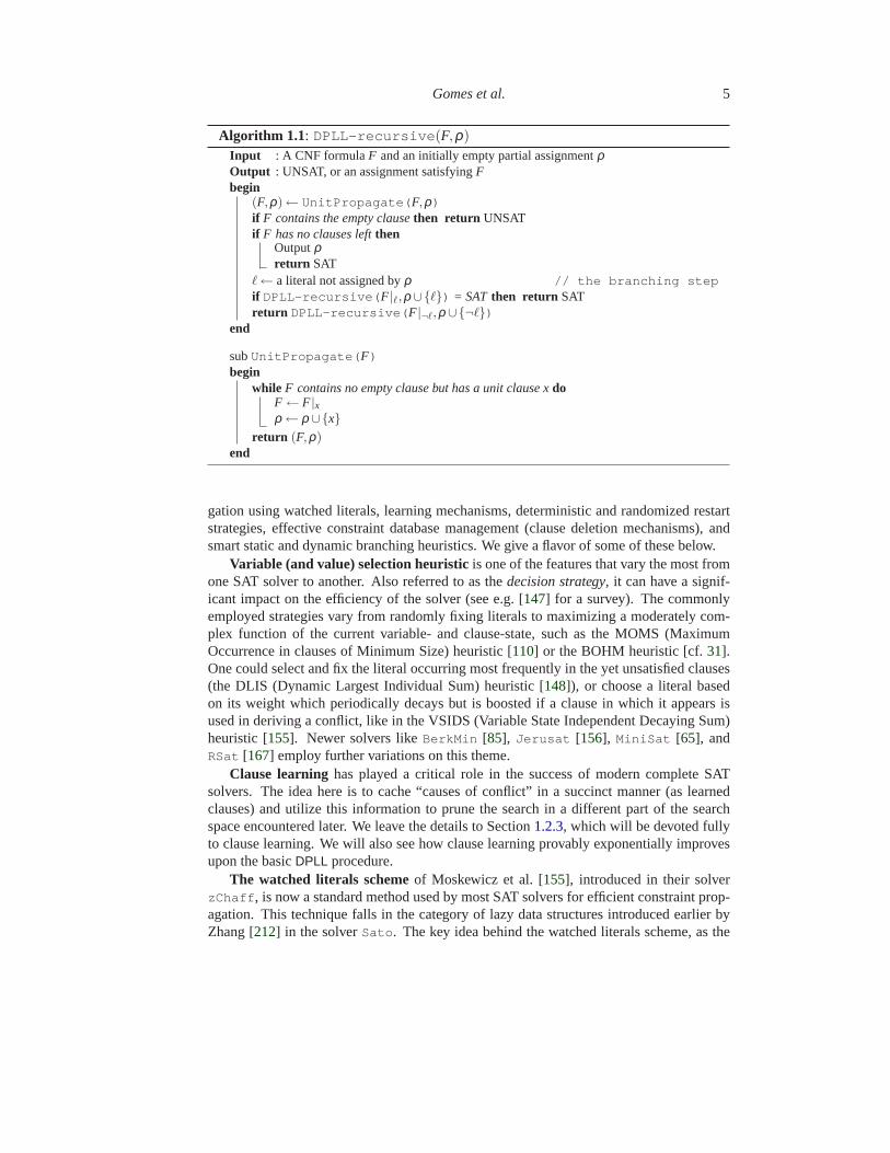


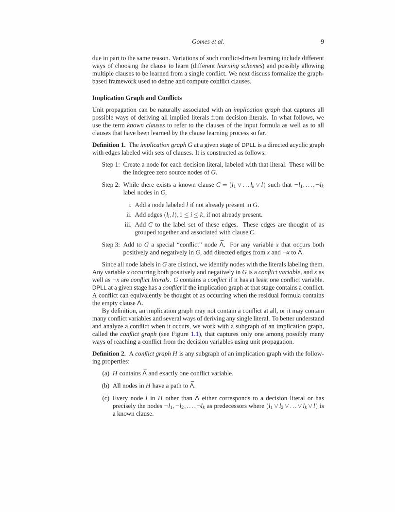


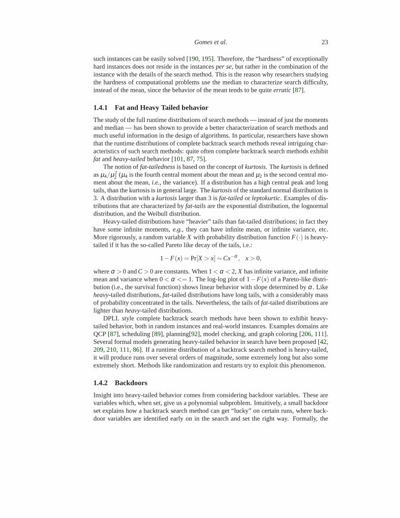


![Solving difficult instances of boolean satisfiability in ...web.eecs.umich.edu/~imarkov/pubs/jour/tcad03-symJ.pdf[21] (DP/DLL) solvers and their derivatives. For example, a recent](https://static.documents.pub/doc/80x56/6074fe8b4ae27e21a1166213/solving-difficult-instances-of-boolean-satisfiability-in-webeecsumicheduimarkovpubsjourtcad03-symjpdf.jpg)


