Saturn’s Rings at True Opposition Author(s): Richard G. French, Anne Verbiscer, Heikki Salo, Colleen McGhee, and Luke Dones Source: Publications of the Astronomical Society of the Pacific, Vol. 119, No. 856 (June 2007), pp. 623-642 Published by: The University of Chicago Press on behalf of the Astronomical Society of the Pacific Stable URL: http://www.jstor.org/stable/10.1086/519982 . Accessed: 19/05/2014 14:05 Your use of the JSTOR archive indicates your acceptance of the Terms & Conditions of Use, available at . http://www.jstor.org/page/info/about/policies/terms.jsp . JSTOR is a not-for-profit service that helps scholars, researchers, and students discover, use, and build upon a wide range of content in a trusted digital archive. We use information technology and tools to increase productivity and facilitate new forms of scholarship. For more information about JSTOR, please contact [email protected]. . The University of Chicago Press and Astronomical Society of the Pacific are collaborating with JSTOR to digitize, preserve and extend access to Publications of the Astronomical Society of the Pacific. http://www.jstor.org This content downloaded from 195.78.109.69 on Mon, 19 May 2014 14:05:17 PM All use subject to JSTOR Terms and Conditions
Transcript
Saturn’s Rings at True OppositionAuthor(s): Richard G. French, Anne Verbiscer, Heikki Salo, Colleen McGhee, and Luke DonesSource: Publications of the Astronomical Society of the Pacific, Vol. 119, No. 856 (June 2007),pp. 623-642Published by: The University of Chicago Press on behalf of the Astronomical Society of the PacificStable URL: http://www.jstor.org/stable/10.1086/519982 .
Accessed: 19/05/2014 14:05
Your use of the JSTOR archive indicates your acceptance of the Terms & Conditions of Use, available at .http://www.jstor.org/page/info/about/policies/terms.jsp
.JSTOR is a not-for-profit service that helps scholars, researchers, and students discover, use, and build upon a wide range ofcontent in a trusted digital archive. We use information technology and tools to increase productivity and facilitate new formsof scholarship. For more information about JSTOR, please contact [email protected].
.
The University of Chicago Press and Astronomical Society of the Pacific are collaborating with JSTOR todigitize, preserve and extend access to Publications of the Astronomical Society of the Pacific.
http://www.jstor.org
This content downloaded from 195.78.109.69 on Mon, 19 May 2014 14:05:17 PMAll use subject to JSTOR Terms and Conditions
Publications of the Astronomical Society of the Pacific, 119: 623–642, 2007 June� 2007. The Astronomical Society of the Pacific. All rights reserved. Printed in U.S.A.
Received 2007 March 9; accepted 2007 May 19; published 2007 June 25
ABSTRACT. On 2005 January 14, the Saturn system was observed at true opposition with the planetary cameraof the Wide Field Planetary Camera 2 (WFPC2) on the Hubble Space Telescope. This was the culmination ofnearly a decade of similar UBVRI observations, yielding a uniform set of over 400 high spatial resolution andphotometrically accurate radial profiles of the rings that spans the full range of ring inclinations and solar phaseangles accessible from the Earth. Using a subset of these images at similar effective ring opening angles
, we measured the normalized ring reflectivity over broad regions of the A, B, and C rings as aB ∼ �23� I/Feff
function of solar phase angle and wavelength. There is a strong surge in brightness near opposition. To measurethe width and amplitude of the opposition effect, we fitted two models to the observations: a simple four-parameterlinear-exponential model and a more complex model (B. Hapke) that incorporates a wavelength-dependentdescription of the coherent backscatter opposition effect, as well as the shadow-hiding opposition effect by aparticulate surface. From fits to the linear-exponential model, the half-width at half-maximum for the rings is∼0.1� at BVRI wavelengths, increasing to ∼0.16� and ∼0.19� for the A and B rings, respectively, in the U filter(338 nm). To assess the contribution of the shadowing of ring particles by each other to the opposition surge,we used Monte Carlo simulations of dynamical models of the rings for a variety of optical depths and particlesize distributions, both with and without self-gravity. Multiple scattering is very weak at low phase angles, andthus these simulations are nearly wavelength independent. The interparticle shadow-hiding opposition surgeincreases in strength with ring optical depth and with broadened size distributions. Self-gravity produces wakesthat somewhat complicate the picture, because mutual shadowing by wakes is strongly dependent on illuminationand viewing geometry. The observed opposition surge in the rings is much stronger and narrower than that causedby interparticle shadowing. We examined regional variations in the opposition surge across the A, B, and C ringsusing linear-exponential model fits. Some of these are most easily explained on the basis of optical depth, volumefilling factor, and the relative width of the particle size distribution. The opposition effect for the A, B, and Crings is substantially narrower than for two nearby icy satellites, Mimas and Enceladus, indicating that they havedistinctly different surface properties.
1. INTRODUCTION
On 2005 January 14, in a rare cosmic alignment, the Earthpassed directly between Saturn and the Sun. Viewed from Sat-urn, this resulted in a transit of the Earth across the center ofthe solar disk. From the Earth, this moment provided an op-portunity to observe the Saturn system at true opposition. Using
the planetary camera (PC) of the WFPC2 on the Hubble SpaceTelescope (HST), we imaged Saturn’s rings at near-zero solarphase angle, the culmination of nearly a decade of such ob-servations spanning more than a full Saturn season, beginningshortly after the 1995–1996 ring plane crossings (southernspring on Saturn) and continuing past Saturn’s southern sum-mer solstice in 2002. Collectively, these observations provide
This content downloaded from 195.78.109.69 on Mon, 19 May 2014 14:05:17 PMAll use subject to JSTOR Terms and Conditions
a uniform set of high spatial resolution and photometricallyaccurate radial profiles of the rings over the full range of ringinclinations and solar phase angles accessible from the Earth.
Variations of ring brightness with ring tilt, phase angle, andwavelength reveal both the scattering properties of individualring particles as well as their collective spatial and size distri-butions. An important test of our understanding of the physicaland dynamical characteristics of Saturn’s rings is our abilityto account for the strong surge in ring brightness near oppo-sition. As a step toward this goal, we present recent HST mea-surements of the opposition surge of the A, B, and C rings forsolar phase angles a from nearly zero to ≤6.38�. In § 2, webriefly summarize previous observations and the HST resultsused for this study. Then in § 3, we develop a suite of modelsfor the opposition surge. We begin by fitting a simple linear-exponential model to the phase-angle–dependent brightness ofselected regions in the A, B, and C rings, primarily to quantifythe wavelength-dependent width and amplitude of the narrowopposition peak. Next, we fit Hapke (2002) photometric modelsfor the opposition effect, which account for shadow hiding atthe surfaces of individual ring particles and for coherent back-scatter, the enhancement of the emergent scattered intensityresulting from constructive interference of the incident andscattered waves. To account for shadowing between ring par-ticles, which is neglected in the Hapke (2002) prescription, wecompare ring brightness measurements to Monte Carlo ray-tracing predictions based on N-body dynamical simulations fora variety of ring optical depths and particle size distributions.We then investigate radial variations in the opposition effectacross the entire ring system and compare our results withmeasurements of the opposition effect for Mimas and Ence-ladus. Finally, in the last section, we discuss our key findings,compare our results to recent findings from Cassini observa-tions, and present our conclusions.
2. OBSERVATIONS
2.1. Previous Results
The strong brightening of Saturn’s rings near opposition hasbeen known for many years. Early investigators relied primarilyon photodensitometry of photographic plates, with varying re-sults. Franklin & Cook (1965) presented the first detailed anal-ysis of observations of the opposition effect in Saturn’s rings,based on a large series of two-color photographic plates ob-tained in 1959. They found some evidence for a slight wave-length dependence of the phase curve, a finding supported byIrvine & Lane (1973) using observations taken during the 1963apparition, and by Lumme & Irvine (1976) from an extensivestudy of over 200 photographic plates obtained during a30 year period. These purported wavelength trends were con-tradicted by Lumme et al. (1983), who observed the B ring atsmall tilt angle and found no wavelength dependenceB ∼ 6�for the phase function for phase angles . They con-a 1 0.26�cluded that the opposition effect resulted from mutual shad-
owing of ring particles in a classical many-particles-thick layer,with a very low volume filling factor, although Brahic (1977),Goldreich & Tremaine (1978), and Cuzzi et al. (1979) hadestablished that the rings should be one or only a few particlesthick and consequently have a relatively high volume fillingfactor, a conclusion supported by later, more detailed studies(Salo 1987, 1992; Wisdom & Tremaine 1988; Richardson 1994;Salo et al. 2004; Karjalainen & Salo 2004). Salo & Karjalainen(2003, henceforth SK2003) showed that the apparent contra-diction between the observations and the simulations is largelyremoved when the ring particle size distribution and the de-pendence of the vertical scale height on particle size are takeninto account.
All of the foregoing studies ignored the potentially largecontribution of coherent backscatter to the strong oppositionsurge at very low phase angles. The coherent backscatter op-position effect (CBOE) has been studied extensively, both the-oretically and in the laboratory (Akkermans et al. 1988; Shkur-atov 1988; Muinonen et al. 1991; Mishchenko 1992; Nelsonet al. 2000), and Hapke (2002) developed a detailed model forthe bidirectional reflectance of a surface, accounting both forcoherent backscatter and shadow hiding due to surface mi-crostructure. The models of CBOE are highly idealized, andthus far, agreement between the theory and experiments hasbeen elusive (see Shepard & Helfenstein 2007 for a review).Poulet et al. (2002) presented the first detailed analysis of highspatial resolution, photometrically precise measurements of theopposition effect in Saturn’s rings, using Hubble Space Tele-scope images. They estimated ring particle roughness and po-rosity by analyzing the observed ring phase curves in terms ofintraparticle shadow hiding, multiple scattering, and coherentbackscattering, but they ignored mutual shadowing betweenparticles. Their observations were restricted to phase angles10.3� and thus required extrapolation of the steep oppositionbrightening to zero phase angle, undersampling the narrowestpart of the solar phase curve. Here we present HST measure-ments that remedy those limitations by spanning the full rangeof phase angles visible from the Earth.
2.2. HST Observations
The viewing and illumination geometry of the HST ringobservations is illustrated in Figure 1, which shows the vari-ation of the solar phase angle and the Saturnocentric declina-tions of the Earth (B) and Sun ( ) over the period of obser-′Bvation. During each of nine apparitions (labeled by HST cyclenumbers 6–13), we obtained UBVRI images of the rings withthe WFPC2 PC camera for several HST “visits,” chosen tosample the full range of accessible solar phase angles, butconcentrated near opposition. Table 1 provides additional de-tails about the observations. For each data set, identified byHST program ID, cycle number, and visit number, we list thedate of each visit, the ring plane opening angles B and , the′Beffective ring opening angle (defined below), the averageBeff
This content downloaded from 195.78.109.69 on Mon, 19 May 2014 14:05:17 PMAll use subject to JSTOR Terms and Conditions
Fig. 1.—Geometry of HST observations of Saturn’s rings. The opening angleof the rings as viewed from the Sun (dashed line) was nearly zero in 1996,when the first of nine Saturn apparitions was observed using WFPC2. Saturnreached southern summer solstice in late 2002. The ring opening angle as seenfrom the Earth (dotted line) is modulated by the Earth’s annual motion relativeto Saturn’s inclined orbit. The solar phase angle is shown at the top of thefigure, approaching zero at each opposition and reaching a maximum of justover 6� near quadrature. Filled circles mark the geometric circumstances ofthe full set of HST observations. For this study of the opposition effect, wemake use of data from HST cycles 10–13, for which the ring opening anglewas nearly constant and close to its maximum value as seen from the Earthand the Sun.
solar phase angle a, and the number of UBVRI images takenof the east (E) and west (W) ansae during each visit.1 Becauseof the relative inclinations of Earth’s and Saturn’s orbits, theminimum phase angle visible at each opposition was limitedto for cycles 6–9 and reached 0.07� during cyclea 1 0.25�12. During cycle 13 in 2005 January, we observed the ringsat true opposition, with . As discussed below, thea ∼ 0.01�finite angular radius of the Sun of 0.029� as seen from Saturnsets an effective lower limit on the phase angle near trueopposition.
For each of the more than 400 PC images in our data set,we began with the pipeline-processed data from the Space Tele-scope Science Institute. We corrected the images for geometricdistortion and converted the measured signal to a wavelength-dependent normalized reflectivity , defined as the ratio ofI/Fring surface brightness I to that of a perfect, flat, Lambertsurface at normal incidence , where is the solarpF(l)/p pF(l)flux density, or irradiance at Saturn, at wavelength l. To correctfor low-level scattered light, we applied a low-pass deconvo-lution filter to the data, resulting in a “compensated” image
, an approximation to the ideal deconvolved image.(I/F)comp
The deconvolution procedure has a very minor effect for the
1 The field of view of the PC chip of WFPC2 is not large enough to containthe full ring system and its attendant nearby small moons, and we thereforetargeted the east and west ring ansae separately during most visits.
present investigation. For additional details of the completeprocessing procedure, see Cuzzi et al. (2002).
We used the Encke division as a geometric reference andsolved for the center of Saturn in each image. Then, to enableeasy comparison of the radial ring profiles, we reprojected eachimage onto a rectilinear grid as a function of ring plane(r, v)radius r and ring longitude v, first rebinning each image pixelinto subpixels and then redistributing them into cells20 # 20in with a resolution of 100 km in r and 0.1� in v. Radial(r, v)profiles of ring reflectivity were obtained by deter-(I/F) (r)corr
mining the median value at each r over a longitude range of�5� centered on each ring ansa.
As a final step in the processing, we define the geometricallycorrected (see Dones et al. 1993; Cuzzi et al. 2002; FrenchI/Fet al. 2007) as
′m � m( ) ( )I/F p I/F , (1)corr comp′2m
where and . The effective ring el-′ ′m { F sin BF m { F sin B Fevation angle is defined byBeff
′2mmm { F sin B F p . (2)eff eff ′m � m
This correction factor for observations at slightly differentB and is exact for an optically thick, singly scattering, many-′Bparticle-thick ring and is a reasonable approximation for mul-tiple scattering (Lumme 1970; Price 1973), although it may beless applicable at very low optical depths. During a single HSTcycle, is roughly constant, although B and may vary′B Beff
somewhat, as shown in Table 1.Ring brightness varies with both ring tilt and solar phase
angle. Since our primary interest here is in the opposition surge,rather than the well-known “tilt effect” (Cuzzi et al. 2002), werestrict our attention in this paper to data from cycles 10–13.These images sample the full range of available phase anglesat nearly the same ring opening angle, minimizing the varia-tions in with ring tilt. Cycles 10–12 were all observed(I/F)corr
at near �26�, and cycle 13, at , is includedB B p �22.87�eff eff
because these images were acquired at the lowest phase angleof the entire set of observations.
Tables 2–4 present measurements from cycles 10–13 of theaverage over three ring regions as a function of wave-(I/F)corr
length (the UVBRI filters respectively correspond to WFPC2filters F336W, F439W, F555W, F675W, and F814W) and solarphase angle.2 The C ring data (Table 2) are averaged over aradial region (78,000–83,000 km) where the reflectivity is fairlyuniform, excluding most of the prominent ringlets and plateausin this ring. Typical uncertainties in for the C ring are(I/F)corr
2 The phase angles in Tables 2–4 are measured with respect to the centerof the Sun. We account for the Sun’s finite angular size in our models byconvolution over the limb-darkened solar image as viewed from Saturn.
This content downloaded from 195.78.109.69 on Mon, 19 May 2014 14:05:17 PMAll use subject to JSTOR Terms and Conditions
�0.002 for F555W. For the B ring (Table 3), we averagedover the range 100,000–107,000 km, chosen to avoid the sat-urated region of the B ring in the F336W cycle 13 zero-phaseimage. The radial range for the A ring of 127,000–129,000 km(Table 4) was chosen to match the region of maximum observedazimuthal brightness asymmetry in the A ring (French et al.2007). Typical measurement uncertainties in for the B(I/F)corr
and A ring data are �0.005 (F555W). The effective wave-lengths for each filter, listed in Tables 2–4, were corrected forinstrumental response, solar spectrum, and the average ringspectrum (Cuzzi et al. 2002).
3. MODELING THE OPPOSITION SURGE
The changing brightness of the rings with phase angle andring tilt depends on the shadowing of ring particles by eachother, the regolith structure of the ring particles themselves,and the degree of multiple scattering, both between ring par-
ticles and within the particles’ regolith. A complete descriptionof ring scattering properties would involve a comparison ofobservations over the full range of solar phase angles and ringtilts, from radio wavelengths to the UV. As a first step, wefocus here on quantifying the width and amplitude of the strongand narrow opposition surge itself at visual wavelengths.
3.1. Linear-Exponential Model Fits
We begin with a simple analytic representation of the sharp,narrow opposition surge and the more gradual slope at largerphase angle. Following Poulet et al. (2002) and for eventualcomparison with Cassini results (Deau et al. 2006; Nelson etal. 2007), we adopt a simple four-parameter combined linearand exponential model commonly used for asteroid and satellitenear-opposition phase curves:
�a/df (a) p a e � b � ka, (3)
This content downloaded from 195.78.109.69 on Mon, 19 May 2014 14:05:17 PMAll use subject to JSTOR Terms and Conditions
Note.— , 434, 549, 672, 798 nm, corresponding to the filters F336W, F439W, F555W,l p 338eff
F675W, and F814W, respectively (Cuzzi et al. 2002).
(Piironen et al. 2000; Muinonen et al. 2002; Kaasalainen et al.2003), where is the point-source model at phasef (a) (I/F)corr
angle a, a is the height of the narrow opposition peak, b is thebackground intensity, d is the width of the opposition peak,and k is the slope of the linear component of the model.
The solar phase angle a given in Tables 2–4 corresponds tothe instantaneous angle between the center of the Sun and thecenter of the Earth, as seen from Saturn. Terrestrial parallax iscompletely negligible, and therefore it is not important to takeinto account the HST orbital position at the time of each ex-posure. However, the Sun is not a point source, and the solarphase angle of the illumination on Saturn’s rings varies acrossthe solar disk. An accurate model calculation for the predictedring brightness thus involves convolving the point-sourcephase-angle–dependent model brightness over the limb-dark-
ened disk of the solar image. We make use of a simple one-parameter solar limb-darkening model:
2 blˆ ˆI (r) p (1 � r ) (4)l
(Hestroffer & Magnan 1998), where is the normalizedˆI (r)l
limb-darkened solar intensity, is the normalized radial co-rordinate of the solar disk, and is a wavelength-dependentbl
constant chosen to fit the observed solar limb-darkening profile.From Table 2 of Hestroffer & Magnan (1998), we adopt thevalues , 0.65, 0.51, 0.39, and 0.324 for the UBVRIb p 0.80l
filters, respectively, for all convolutions with the solar image.We fitted equation (3) to the data in Tables 2–4 for each ring
region and filter and computed the model for each(I/F)corr
observation by convolving over the limb-darkened disk of the
This content downloaded from 195.78.109.69 on Mon, 19 May 2014 14:05:17 PMAll use subject to JSTOR Terms and Conditions
Note.— , 434, 549, 672, 798 nm, corresponding to the filters F336W, F439W, F555W,l p 338eff
F675W, and F814W, respectively (Cuzzi et al. 2002).
solar image, using
f (a, Q)I (Q) dQ∫ l
model (I/F) p , (5)corrI (Q) dQ∫ l
where is the limb-darkened solar intensity, is theI (Q) a(Q)l
phase angle, and the integrations are carried out over the solidangle of the solar image as seen from a given point in thedQ
rings.The results of the least-squares fits are given in Table 5. We
also include , the amplitude of the exponential oppositiona/bsurge a relative to the mean intensity b, and the normalizedbackground slope , corresponding to the fractional changek/bin ring brightness, per degree of phase angle, of the linear termin the model. For comparison with other model fits, we also
list the half-width at half-maximum and R,HWHM p d ln 2the rms residual between the observed and model . The(I/F)corr
model fits are plotted in Figure 2 (left column) for each ringregion. For clarity, the phase angle is shown on a logarithmicscale. A vertical dashed line indicates the angular radius of thesolar disk as seen from Saturn, and the flattening of the modelcurves at smaller phase angles results primarily from the func-tional form of the model (eq. [3]), and to a lesser extent fromconvolution with the solar image. The fits are quite acceptable,given the simple form of the four-parameter model function.The models uniformly underestimate the lowest phase angleobservations, and the observations at phase angles falla 1 1�more linearly on these plots than the model curves, but theoverall trends are well matched.
The wavelength dependence of the width, amplitude, and slope
This content downloaded from 195.78.109.69 on Mon, 19 May 2014 14:05:17 PMAll use subject to JSTOR Terms and Conditions
Note.— , 434, 549, 672, 798 nm, corresponding to the filters F336W, F439W, F555W,l p 338eff
F675W, and F814W, respectively (Cuzzi et al. 2002).
of the linear-exponential model fits is shown in Figure 3. For theoptically thin C ring, the HWHM of the narrow surge (Fig. 3a)is nearly independent of wavelength, with an average value of0.10�. In contrast, at F336W the B ring HWHM (0.192�) is nearlydouble that for F555W (0.099�) and longer wavelengths; the Aring is an intermediate case, also showing a wider surge in theU filter (0.158�) than the average value (0.09�) at longer wave-lengths. The amplitude (Fig. 3b) has a weak wavelengtha/bdependence, with the dark and optically thin C ring showingthe strongest opposition surge ( ), and the opaque Ba/b ≈ 0.6ring the weakest ( ). The normalized slope (Fig. 3c)a/b ≈ 0.4shows a similar pattern, with steeper slopes at short wave-lengths and generally weaker slopes for the more opaque ringregions. We return to these results below.
We find that the opposition surge is much narrower (∼0.1�–
0.2� HWHM) than Poulet et al. (2002) derived from their anal-ysis of HST observations during the 1997–1998 apparition. Forthe A, B, and C rings, they obtained HWHMs ranging from0.41� to 0.67�, with no clear wavelength dependence. However,the minimum phase angle of their observations was 0.3�, sub-stantially greater than for our data (see Table 1). From fits tosubsets of our current measurements, we find that the fittedHWHM of the narrow opposition surge depends quite stronglyon the inclusion of the 2005 January 14 measurements obtainedat true opposition. When these observations were excluded fromthe fits, the HWHM increased from 0.1�–0.2� to 0.16�–0.25�.Similarly, when we fitted only data for which , thea 1 0.3�HWHM ranged from 0.33�–0.39�, 0.41�–0.56�, and 0.36�–0.49�for the C, B, and A rings, respectively, roughly comparable tothe Poulet et al. (2002) results from HST measurements at
This content downloaded from 195.78.109.69 on Mon, 19 May 2014 14:05:17 PMAll use subject to JSTOR Terms and Conditions
Note.— , 434, 549, 672, 798 nm, corresponding to the filters F336W, F439W, F555W,l p 338eff
F675W, and F814W, respectively (Cuzzi et al. 2002).1 HWHM p half-width at half-maximum.2 R p rms residual of .(I/F)corr
smaller (∼�10�) than our present data set. These resultsBeff
show that the true opposition measurements are substantiallybrighter than a simple extrapolation to low phase angles fromhigher phase observations would suggest, and that the near-zero phase measurements provide a strong constraint on theactual width of the opposition surge.
3.2. Hapke Model Fits
The linear-exponential model has the virtue of analytic sim-plicity, providing useful estimates of the amplitude and thewidth of the core of the opposition surge itself, as well as themore gradual decline characteristic of the observations at largerphase angles. We next turn to the Hapke (2002) model, whichincorporates a wavelength-dependent CBOE based on the the-oretical predictions of Akkermans et al. (1988) and an explicitrepresentation of the shadow-hiding opposition effect (SHOE)by a particulate surface. The Hapke (2002) model has beenapplied to satellite measurements from these same HST ob-servations (Verbiscer et al. 2007) and combined with Voyagerspacecraft measurements (Verbiscer et al. 2005) to quantify theopposition surge on Saturn’s satellites, which brighten consid-erably at true opposition (Verbiscer et al. 2007).
For each ring and filter in Tables 2–4, we fitted the Hapke(2002) model using the nonlinear least-squares algorithm de-veloped by Helfenstein (1986) and described by Helfenstein etal. (1991), modified to accommodate anisotropic multiple scat-tering as described by Verbiscer et al. (2005). Our model fitsappear in the right-hand column of Figure 2, and all parametersderived from the fits are listed in Table 6. These fits haveconsistently lower rms residuals per degree of freedom thanthe linear-exponential fits, and they do a better job of capturingboth the very low phase angle measurements and the falloff
in for , which is more gradual than implied by(I/F) a 1 1�corr
the linear-exponential model.The Hapke (2002) model is characterized by parameters that
include the single-scattering albedo , the single-particle�o
phase function asymmetry parameter g, and the width h andamplitude of the SHOE and CBOE. For completeness, weBo
also account for the mean topographic slope angle , using thev
formalism of Hapke (1984, 1993), which was derived for anygeneral reflectance function. Although the phase angle coverageof the HST observations ( ) is well suited toa p 0.01�–6.4�constrain the angular widths of both the SHOE and CBOE, therestriction to Earth-based measurements somewhat compro-mises our ability to determine parameters such as g and ,v
which are constrained primarily by data obtained at larger phaseangles. As noted by Shepard & Helfenstein (2007), photometricroughness tends to decrease with increasing albedo. This trendis evident in the B ring, for which falls off from ∼41� atv
short wavelengths to ∼27� at longer wavelengths, where thealbedo is higher. At 549 nm, we find that the roughness of allrings is higher than that determined by Poulet et al. (2002) forthe C ring and for Mimas ( ; Verbiscer & Veverka 1992),v p 30�the innermost of Saturn’s “classical” satellites. Our values of
are significantly lower than those ( ) determined¯ ¯v v ∼ 60�–70�by Poulet et al. (2002); however, no firm conclusions about theroughness of ring particles can be drawn from fits to obser-vations made at phase angles no larger than .a p 6.4�
The wavelength dependence of several Hapke (2002) modelparameters is shown in Figure 3. The single-scattering albedo
increases with wavelength for all rings (Fig. 3d), although�o
the increase is much more pronounced for the A and B ringsthan for the C ring. The albedo of the optically thin C ring ismuch smaller than that of the optically thick A and B rings.
This content downloaded from 195.78.109.69 on Mon, 19 May 2014 14:05:17 PMAll use subject to JSTOR Terms and Conditions
Fig. 2.—Model fits to HST WFPC2 observations (Tables 2–4) of the opposition effect for selected regions in Saturn’s C, B, and A rings. The left column showsthe results of the linear-exponential (LINEXP) model fits from Table 5, and the right column shows the Hapke (2002) model fits given in Table 6. The colored linesand symbols (violet to red) correspond to the F336W, F439W, F555W, F675W, and F814W filters, respectively. The plotted phase angles are measured with respectto the center of the solar image, and the finite size of the Sun was taken into account in the models by convolution over the limb-darkened solar disk (eq. [5]). Thevertical dashed lines mark the angular radius of the Sun as viewed from Saturn ( ), setting the approximate effective minimum solar phase angle of thea p 0.029�Sun
measurements. The linear-exponential models match the observations reasonably well, given only four free parameters, although they consistently underestimate thelowest ring brightness at minimum phase angle, and they deviate systematically from the measurements near (where they underestimate the true ring brightness)a p 0.5�
and near (where they overestimate the true brightness). The Hapke (2002) models show no such systematic deviations from the measurements.a p 2�
This content downloaded from 195.78.109.69 on Mon, 19 May 2014 14:05:17 PMAll use subject to JSTOR Terms and Conditions
Fig. 3.—Wavelength dependence of linear-exponential (LINEXP) and Hapke (2002) model fits to HST WFPC2 observations of the opposition effect for selectedregions in Saturn’s C, B, and A rings, plotted as a function of the effective wavelength of the WFPC2 UBVRI filters. (a)–(c): HWHM, amplitude, and normalizedslope from the LINEXP fits (Table 5); (d)–(i): selected parameters from the Hapke (2002) model fits (Table 6).
The asymmetry parameter g is the average cosine of the scat-tering angle V: and . While g does notg { Acos VS V { p � a
vary significantly with wavelength for the A ring (Fig. 3e), theB ring backscatters more strongly at longer wavelengths, from
at 338 nm to at 672 nm. Strictly speak-g p �0.28 g p �0.50ing, these model parameters apply to the individual grains inthe regolith of a typical ring particle, and not to the particle asa whole.
The transparency of regolith grains affects their ability tocast shadows, and thus the SHOE amplitude (Fig. 3f) is directlyrelated to particle opacity ( for transparent particles andB p 0oS
for opaque grains). For all rings, generally decreasesB p 1 BoS oS
with wavelength, indicating that particles are more transparentat longer wavelengths. The SHOE angular width is related tohS
regolith porosity and is only weakly dependent on wavelength,except in the C ring at 338 nm, where it is somewhat higher
than at longer wavelengths (Table 6). If we assume a uniformparticle size distribution, then , where P is theh p (�3/8) ln PS
porosity (Hapke 1986). Under this assumption, all of the valuesof in Table 6 imply that porosities of ring particle regolithshS
are very high, ranging from 93% to 99%. The CBOE amplitude(Fig. 3g) does not show a strong wavelength dependence,BoC
except for an increase at short wavelengths for the C ring.The opacity of regolith grains affects not only the shadow-
hiding amplitude, but the width of the coherent backscatteropposition surge as well. According to Hapke (2002), theCBOE HWHM is given by , where L is0.36l/2pL ≈ 0.72hC
the transport mean free path, the average distance a photontravels before being deflected by a large angle (∼1 rad). In thispicture, the CBOE HWHM should increase with wavelengthfor a constant L, but this is not what we see. Instead, we findthat the Hapke CBOE HWHM (Fig. 3h) is largest for all rings
This content downloaded from 195.78.109.69 on Mon, 19 May 2014 14:05:17 PMAll use subject to JSTOR Terms and Conditions
Notes.— , 434, 549, 672, 798 nm, corresponding to the filters F336W, F439W, F555W, F675W,l p 338eff
and F814W, respectively (Cuzzi et al. 2002). p single-scattering albedo (�0.02), p macroscopic¯� vo
roughness (�4), p SHOE width (�0.003), p SHOE amplitude (�0.03), p CBOE width # 103h B hS oS C
(�0.03), p CBOE amplitude (�0.07), p Henyey-Greenstein asymmetry parameter (�0.04), pB g LoC
transport mean free path (�0.7), HWHMp CBOE HWHM (�0.002), and p rms residual.R
at the lowest wavelength (338 nm), falling sharply and thenremaining relatively constant at ∼0.055� with increasing wave-length from 439 to 798 nm. Nelson et al. (2002) suggest thatthe wavelength dependence of and the CBOE HWHM mayhC
require a broader range of wavelengths than observed here inorder to be seen. In addition, Petrova et al. (2007) invoke athird mechanism, the near-field effect, to explain why the pre-dicted spectral behavior of the opposition effect is not observed.The near-field effect is produced by the inhomogeneity ofwaves in the immediate vicinity of low- to moderate-albedoregolith grains that are comparable in size to the wavelength.If we assume a uniform particle size distribution, according toHelfenstein et al. (1997) we can estimate particle sizes fromour Hapke (2002) parameters. The particle radius is given by
, and using the values in Table 6, wer p 3.11� (1 � g)h LP o S
find that grains on C ring particles are an order of magnitudesmaller ( mm) than those on A and B ring particles.r ∼ 0.16P
We measure the broadest CBOE widths (and HWHM) wherethe single-scattering albedo ranges from 0.1 (for the C ring) to0.6 for the B ring at 338 nm, so it is possible that this thirdphenomenon may act in addition to coherent backscatter andclassical shadow hiding to produce the opposition effect ob-served in Saturn’s rings.
From our Hapke (2002) fits to the HST data, we find thatthe transport mean free path increases with wavelength for allrings, from mm at 338 nm to ∼45 mm at 798 nm forL ∼ 11the A and B rings, with somewhat higher values in the darkerC ring (Table 6, Fig. 3i). Our measurements are consistent withthose of Hapke et al. (2006b), who found mm (whereL � 10the reflectance of the ring was low) to mm (where itL � 40was high) in their analysis of Cassini VIMS (Visual and In-
frared Mapping Spectrometer) data at wavelengths between 1and 5 mm. The near-field effect may play an important rolehere, since it is most efficient in more compact structures ofwavelength-sized scatterers at distances comparable to thewavelength, and the transport mean free path is smallest at338 nm, the shortest wavelength observed, where the albedoof all the rings is low to moderate. A fuller consideration ofthe interplay of these effects must await additional observationsover a broader range of wavelengths and phase angles.
3.3. Monte Carlo Simulation of Interparticle Shadowing
The Hapke (2002) model accounts for shadowing withinthe regolith of a spherical ring particle, but does not explicitlyinclude shadowing between ring particles, which depends onthe particle size distribution and the vertical structure of thering, as well as the slant path optical depth. To assess theimportance of interparticle shadowing, we use dynamical sim-ulations in which the optical depth and the width of the sizedistribution are varied. Although theoretical formulas existfor the mutual shadowing of particles (Lumme & Bowell1981; Hapke 1986), the advantage of our simulations is thatthey account for the partial vertical segregation of differentparticle sizes (SK2003). In these simulations, we adopt theBridges et al. (1984) formula for the velocity-dependent co-efficient of restitution during particle impacts, leading to mod-erately flattened systems with vertical thickness a few timesthe diameter of the largest particles (for an illustration, seeFig. 2 in SK2003).
For simplicity, we first concentrated on models that ignorethe self-gravity of the rings. We adopted a power-law size
This content downloaded from 195.78.109.69 on Mon, 19 May 2014 14:05:17 PMAll use subject to JSTOR Terms and Conditions
Fig. 4.—Comparison of the observed A ring phase curves (plus signs) to the mutual-shadowing opposition effect calculated by photometric Monte Carlo simulations(curves). Dynamical simulations with seven different particle size distributions were conducted, ranging from q p 3 power laws for 0.05–5 m to simulations withidentical 5 m particles. At left, the two extreme size distribution models are compared to observations at different wavelengths. The single-scattering albedos for themodels, indicated in the middle panel, are chosen to fit the observed at . At right, the observations and single-scattering models are normalized toI/F a ≈ 6� a p
. Also shown is the contribution from the adopted power-law phase function alone, amounting to about 1.1 for the interval � to .6.35� a p 0 6.35�
distribution of N particles with and , an�qdN/dr ∝ r q p 3upper particle radius cutoff m, and lower size cutoffsr p 5max
ranging from to 5 m, the latter case correspondingr p 0.05min
to a monodispersion of identical particles.3 In each case, thedynamical optical depth (the total projected surface areatdyn
of ring particles per unit area of the rings) was held fixed at0.5, a typical value for the mid-A ring.
To estimate the contribution of interparticle shadowing tothe opposition phase curves, we use a Monte Carlo methodbased on following a large number of photons through theparticle fields produced by the dynamical simulation. The par-ticle field, with periodic planar boundaries, is illuminated bya parallel beam of photons, and the path of each individualphoton is followed in detail from one intersection with aparticle surface to the next scattering, until the photon escapesthe particle field. The new direction after each scattering isobtained via Monte Carlo sampling of the particle phase func-tion. The brightness at the observing direction is obtained byadding together the contributions of all visible individual scat-terings. Compared to direct Monte Carlo estimates based ontabulating the directions of escaped photons, this indirectmethod gives significantly reduced variance. To suppress thestatistical fluctuations in the dynamical simulations, we av-
3 Although the actual particle size distributions may be somewhat broaderin parts of the rings than in these simulations (French & Nicholson 2000),extending the simulations beyond a size range spanning 2 orders of magnitudewas computationally prohibitive.
erage the photometric results for several individual simulationsnapshots. Because self-gravity was not included, the systemsare homogeneous in the planar direction. We consider the ef-fects of self-gravity at the end of this section.
To describe the angular distribution of scattered light fromthe surface of a ring particle, we adopted a power-law phasefunction:
nP (a) p c (p � a) , (6)power n
where is a normalization constant. For , this givesc n p 3.092n
a good match to the phase function of the inner A ring (Doneset al. 1993); we hereafter refer to this as the power-law phasefunction. In our Monte Carlo simulations, we take into fullaccount partial shadowing of ring particles by each other, andeach scattered photon is followed from its intersection pointon the surface of a particle (in a direction whose probabilityis weighted by the power-law phase function), rather than fromthe particle center. Comparisons of Lambert surface elementscattering and Lambert “sphere” scattering (see § 3.5 inSK2003) show the importance of this refinement.
The results of our simulations are shown in Figure 4. In theleft panel, we compare the observed UBVRI A ring phasecurves (the data from Table 4, plotted as colored symbols) withthe mutual particle shadowing opposition effect calculated fromphotometric Monte Carlo simulations for two extreme size dis-tributions: a power law for 0.05–5 m particles, and aq p 3
This content downloaded from 195.78.109.69 on Mon, 19 May 2014 14:05:17 PMAll use subject to JSTOR Terms and Conditions
Note.—Single-scattering calculations denoted by (ss), HWHM p half-width at half-maximum, and p rms residualRof fit.
monodispersion of 5 m size particles. The opposition surge forthe identical particle case (dashed lines) is quite broad, and the
curve is essentially flat for . For the broader sizeI/F a ! 1�distribution (solid line), the surge is narrowed because of theabundance of relatively small particles, not flattening until
. Following Hapke (1986), this trend can be understooda ! 0.1�as follows. The angular width of the mutual-shadowing op-position surge is determined by the angular width w of thetypical particle shadow cylinder having length L: ,w ≈ ArS/Lwhere , and is the average particle cross1/2ArS p (AjS/p) AjSsection. A typical cylinder has volume and containsAjSL
particles, where n is the number density in the scatteringAjSLnlayer. Setting this to unity for the shadow cylinder gives
, yielding , as found by Hapke (1986).L p 1/AjSn w ≈ nAjSArSIn terms of volume density , where is the averageD p nAV S AV Sparticle volume, . Thus, the width of the surgew p AjSArS/AV SDis proportional to the volume density, with a proportionalityconstant that becomes smaller as the width of the size distri-bution is increased (see Fig. 16 in SK2003).
The Bond albedo for the simulations (Fig. 4b) was chosento fit the observed at . Note that the albedos are(I/F) a ≈ 6�corr
higher for the broad size distribution, even though both modelsassume the same . Because the mutual-shadowing opposi-tdyn
tion effect for identical particles extends to relatively largephase angles (i.e., its angular width is large), a lower albedois needed to match at in this case than for a(I/F) a ≈ 6�corr
broad size distribution, where the opposition effect is confinedto smaller angles.
The results of Monte Carlo simulations for seven differentpower-law size distributions are shown in Figure 4c. For sim-plicity, we ignore multiple scattering, which we show belowto be unimportant in this near-backscattering geometry, and
hence these simulations are effectively wavelength indepen-dent. Here both the observations and the models are normalizedto . The contribution to the normalized phase curvea p 6.35�
from the power-law phase function alone is shown as a dashedline, amounting to about 1.1 for the interval � to 6.35�.a p 0Clearly, the observed opposition surge is substantially sharperand narrower than the single-particle phase function itself.
To quantify these trends more precisely, we fitted the linear-exponential model (eq. [5]) to the Monte Carlo simulationsshown in Figure 4, restricting the phase angle to 25 roughlylogarithmically spaced values between 0� and 6�, comparableto the range covered by our Earth-based observations. Theresults are given in Table 7. For this rather narrow range ofphase angles, the fits matched the simulations quite well, asshown by the very small rms error R. The fitted amplitudes
are nearly independent of albedo (or, equivalently, wave-a/blength), a consequence of the weak contribution made by mul-tiple scattering. For both the 0.05–5 m distribution (a/b ≈
) and the 5 m particle size simulations ( ), the0.22 a/b ≈ 0.09opposition surge amplitude from mutual shadowing is signif-icantly smaller than that of the A ring ( ,a/b p 0.419–0.515from Table 5) for comparable . The HWHM for the 0.05–tdyn
5 m case (∼0.4�) is substantially narrower than the 5 m sim-ulation (∼3.5�), but neither model matches the A ring’s sharpsurge with HWHM p 0.083�–0.158� (Table 5). Also includedin Table 7 are linear-exponential fit results for the seven nor-malized single-scattering simulations shown in Figure 4c. TheHWHM increases from ∼0.4� to ∼3� as the width of the particlesize distribution is reduced from 2 decades (0.05–5 m) to asingle decade (0.5–5 m). Although some jitter is apparent inthe trends, due to the intrinsic granularity of the Monte Carlo
This content downloaded from 195.78.109.69 on Mon, 19 May 2014 14:05:17 PMAll use subject to JSTOR Terms and Conditions
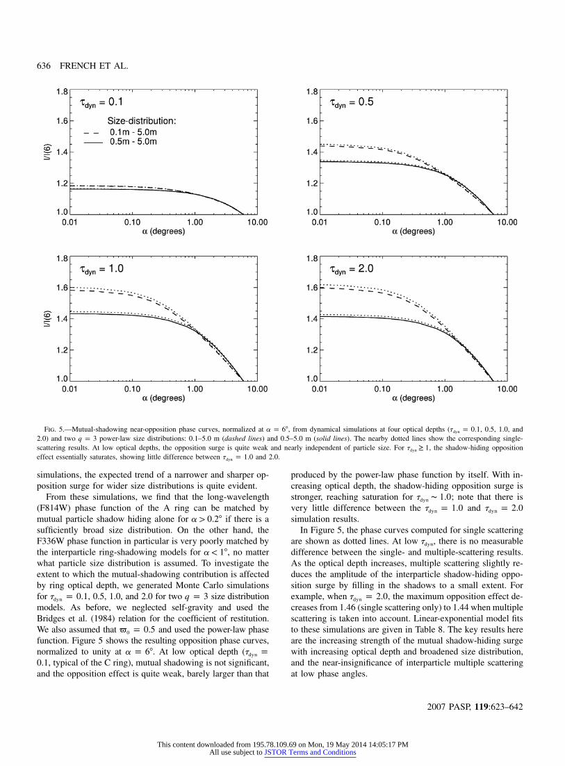
Fig. 5.—Mutual-shadowing near-opposition phase curves, normalized at , from dynamical simulations at four optical depths ( , 0.5, 1.0, anda p 6� t p 0.1dyn
2.0) and two power-law size distributions: 0.1–5.0 m (dashed lines) and 0.5–5.0 m (solid lines). The nearby dotted lines show the corresponding single-q p 3scattering results. At low optical depths, the opposition surge is quite weak and nearly independent of particle size. For , the shadow-hiding oppositiont ≥ 1dyn
effect essentially saturates, showing little difference between and 2.0.t p 1.0dyn
simulations, the expected trend of a narrower and sharper op-position surge for wider size distributions is quite evident.
From these simulations, we find that the long-wavelength(F814W) phase function of the A ring can be matched bymutual particle shadow hiding alone for if there is aa 1 0.2�sufficiently broad size distribution. On the other hand, theF336W phase function in particular is very poorly matched bythe interparticle ring-shadowing models for , no mattera ! 1�what particle size distribution is assumed. To investigate theextent to which the mutual-shadowing contribution is affectedby ring optical depth, we generated Monte Carlo simulationsfor , 0.5, 1.0, and 2.0 for two size distributiont p 0.1 q p 3dyn
models. As before, we neglected self-gravity and used theBridges et al. (1984) relation for the coefficient of restitution.We also assumed that and used the power-law phase� p 0.50
function. Figure 5 shows the resulting opposition phase curves,normalized to unity at . At low optical depth (a p 6� t pdyn
, typical of the C ring), mutual shadowing is not significant,0.1and the opposition effect is quite weak, barely larger than that
produced by the power-law phase function by itself. With in-creasing optical depth, the shadow-hiding opposition surge isstronger, reaching saturation for ; note that there ist ∼ 1.0dyn
very little difference between the andt p 1.0 t p 2.0dyn dyn
simulation results.In Figure 5, the phase curves computed for single scattering
are shown as dotted lines. At low , there is no measurabletdyn
difference between the single- and multiple-scattering results.As the optical depth increases, multiple scattering slightly re-duces the amplitude of the interparticle shadow-hiding oppo-sition surge by filling in the shadows to a small extent. Forexample, when , the maximum opposition effect de-t p 2.0dyn
creases from 1.46 (single scattering only) to 1.44 when multiplescattering is taken into account. Linear-exponential model fitsto these simulations are given in Table 8. The key results hereare the increasing strength of the mutual shadow-hiding surgewith increasing optical depth and broadened size distribution,and the near-insignificance of interparticle multiple scatteringat low phase angles.
This content downloaded from 195.78.109.69 on Mon, 19 May 2014 14:05:17 PMAll use subject to JSTOR Terms and Conditions
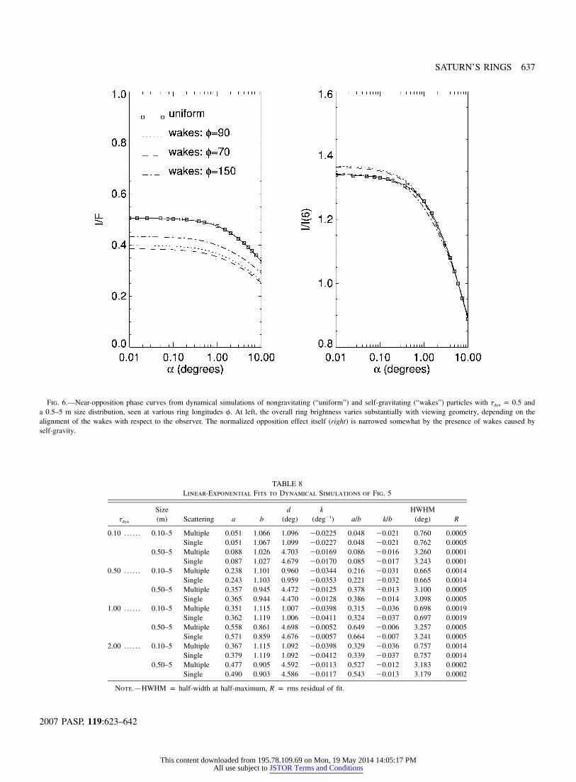
Fig. 6.—Near-opposition phase curves from dynamical simulations of nongravitating (“uniform”) and self-gravitating (“wakes”) particles with andt p 0.5dyn
a 0.5–5 m size distribution, seen at various ring longitudes f. At left, the overall ring brightness varies substantially with viewing geometry, depending on thealignment of the wakes with respect to the observer. The normalized opposition effect itself (right) is narrowed somewhat by the presence of wakes caused byself-gravity.
TABLE 8Linear-Exponential Fits to Dynamical Simulations of Fig. 5
Note.—HWHM p half-width at half-maximum, p rms residual of fit.R
We have neglected self-gravity in all of the foregoing dy-namical simulations, even though it is a crucial ingredient foraccurate models of wake structure and azimuthal brightnessvariations in the rings (SK2003; Salo et al. 2004; French et al.2007), especially in the A ring. Figure 6 compares the phasecurves for nongravitating and self-gravity simulations, seen atvarious ring longitudes. The average ring brightness in the self-gravitating models varies substantially with viewing geometry,depending on the observer’s longitude f (measured in the di-rection of orbital motion from the subobserver point) relativeto the mean wake direction (Fig. 6a). The case cor-f p 70�responds to wakes viewed roughly along their long axis. Linear-exponential fits to these simulations (Table 9) show that thephase curves for the wake models are nearly independent off. However, the amplitude of the surge is weaker when wakesare present ( ) than in the uniform nongrav-a/b p 0.166–0.190itating case ( ), and the width of the shadow-hidinga/b p 0.372opposition peak is much narrower (HWHM p 1.188�–1.300�)than for the uniform case (HWHM p 3.085�). This may bethe result of mutual shadowing between wakes, combined withinterparticle shadowing. Since the 3� HWHM is nearly half ofthe full range of phase angles of the observations, broader phasecoverage from Cassini measurements may be required to deriveaccurate mutual-shadowing effects in the presence of wakes.These examples illustrate the importance of taking into accountthe detailed dynamical environment of the rings when inter-preting phase curves in terms of ring particle properties.
3.4. Regional Variations in the Opposition Surge andComparison with Icy Satellites
To set the stage for more detailed future models of ringscattering properties, we briefly examine the regional variationsin the opposition surge across the A, B, and C rings. For thispurpose, we use the linear-exponential model because it hasthe fewest free parameters and because it provides a reasonablygood match to the results of the more elaborate Hapke (2002)formulation (see Figs. 2 and 3). We performed a suite of fitsto the complete radial ring brightness profiles for the same HSTimages used for Tables 2–4. Figure 7 shows the amplitude,HWHM, and normalized slope at each wavelength obtainedfrom linear-exponential fits to sliding-box averages of the
profiles, binned to a resolution of 300 km in steps of(I/F)corr
100 km in radius. For comparison, a representative (I/F)corr
ring brightness profile and the Voyager PPS (Photopolarimeter
Subsystem) optical depth profile, obtained from the NASAPlanetary Data System Rings Node (Showalter et al. 1996),are also shown, labeled with the major ring regions.
Overall, there is substantial regional variability in the sharp-ness, strength, and wavelength dependence of the oppositionsurge. In the C ring, the detailed variations correlate stronglywith the optical depth variations, especially in the inner and outerregions, where there are ringlets and plateaus with abrupt radialchanges in opacity. If the surface properties of the C ring particlesthemselves are uniform, then the CBOE would be expected tobe similar throughout the ring, whereas interparticle shadow hid-ing depends critically on the ring optical depth, particle sizedistribution, and volume filling factor. The C ring is known tohave a relatively broad particle size distribution: French & Nich-olson (2000) found , cm, m. As weq p 3.1 r p 1 r p 10min max
have seen, this both narrows and sharpens the shadow-hidingopposition surge. In future work, inclusion of ring observationsover a wider range of tilt angles (Salo et al. 2005) will help todisentangle the wavelength-dependent CBOE and shadow hidingin the regolith from interparticle effects.
The opposition effect changes markedly at the boundarybetween the outer C and inner B rings. Over the radial range92,000–99,000 km, which is the least opaque part of the Bring, the amplitude exceeds 0.5, decreasing gradually with in-creasing radius and optical depth. Between 100,000 and107,000 km (the region used for Table 3 and for our fits inFigs. 2 and 3 and Tables 5 and 6), the normalized slope de-creases with increasing ring optical depth. Throughout the Bring, the opposition effect is strongly wavelength dependent,especially at short wavelengths, where the single-scattering al-bedo is also strongly wavelength dependent.4 Compared to theC ring, the B ring particle size distribution is relatively narrowin terms of : , cm, mr /r q p 2.75 r p 30 r p 20max min min max
(French & Nicholson 2000). This tends to weaken the interpar-ticle opposition amplitude (Fig. 4), but this is compensated forin part by the enhanced optical depth of the B ring (Fig. 7).Wakelike structure has been observed in regions of the B ring(French et al. 2007; Colwell et al. 2007), and this might alsocontribute to radial variations in the mutual shadow-hiding com-ponent of the opposition effect.
4 The lone cycle 13 F336W image taken at true opposition was saturatedin the range 107,000–118,000 km, resulting in the gap in coverage for thatfilter in Fig. 7.
This content downloaded from 195.78.109.69 on Mon, 19 May 2014 14:05:17 PMAll use subject to JSTOR Terms and Conditions
Fig. 7.—Radial variations in the amplitude, width, and slope of the opposition surge from linear-exponential model fits to HST WFPC2 observations of Saturn’srings at five wavelengths, taken during cycles 10–13. The colors are the same as in Fig. 2. The amplitude of the opposition effect (top) is nearly independent ofwavelength, except for the F336W filter (violet line), especially in the A and B rings, where the amplitude increases sharply at short wavelengths. (The gap inthe F336W profiles between 107,000 and 118,000 km results from saturation of a unique low-phase-angle cycle 13 image, making the model fits unreliable inthis region for this filter.) The width of the opposition surge varies strongly with ring region at short wavelengths in the A and B rings, and shows strong correlationswith optical depth in the inner and outer C ring. The normalized slope (third panel) is most shallow for the optically thick central B ring. A radial profile of ringbrightness is shown at bottom from a cycle 13 F439W image taken near true opposition ( on 2005 January 14; image u97f1106m). The(I/F) a p 0.0043�corr
horizontal red bars demarcate the radial ranges used for Tables 2–4. The bottom panel shows the Voyager PPS optical depth profile, truncated at becauset p 2.0of limited signal-to-noise ratio at high optical depths.
This content downloaded from 195.78.109.69 on Mon, 19 May 2014 14:05:17 PMAll use subject to JSTOR Terms and Conditions
Fig. 8.—Opposition effect amplitude vs. its angular width at half-maximum(HWHM) due to coherent backscatter (filled circles) and shadow hiding (opencircles) for Saturn’s A, B, and C rings, Mimas (M), and Enceladus (E) at0.55 mm. The CBOE of the ring particles is substantially narrower and on averagea bit stronger than their icy counterparts. The SHOE of the rings is both weakerand narrower than for Mimas and Enceladus, although this may be affectedsomewhat by the relatively narrow range of phase angles ( ) covered bya ! 6.4�
the ring observations.
The Cassini division resembles the C ring in optical depthand possibly in particle size distribution, and these similaritiesare reflected in the opposition effects of these two separatedring regions. The very strong opposition amplitudes at the innerand outer edges of the Cassini division (Fig. 7) are similar tothose in the C ring, and once again there are strong correlationswith optical depth variations. Higher resolution Cassini imagesfor these two regions will be especially valuable in quantifyingthese connections.
The A ring and the inner B ring have comparable opticaldepths, and the overall characteristics of the opposition effectare similar, including significant strengthening and broadeningat short wavelengths. The particle size distribution of the innerA ring ( , cm, m; French & Nich-q p 2.75 r p 30 r p 20min max
olson 2000) is similar as well, and measurements of the strongquadrupole brightness variations (French et al. 2007) indicatethat self-gravity wakes are especially strong in the central Aring region. Figure 7 reveals a striking contrast between theinner and outer A ring opposition effect. Outside of the Enckedivision, the amplitude , much larger than anywherea/b ∼ 0.7else in the A and B rings and comparable to the largest seenin the C ring. The HWHM is a bit narrower here than in theinner A ring as well. These are just the trends expected frominterparticle shadowing for a broad size distribution, and indeedthe outer A ring has a much greater abundance of small particles( , cm, m; French & Nicholsonq p 2.9 r p 1 r p 20min max
2000) than the inner A ring.Verbiscer et al. (2007) used the Hapke (2002) model to de-
scribe the opposition effect of Saturn’s icy satellites from theHST observations summarized in Table 1, and it is instructiveto compare these results with our measurements of the oppo-sition effect of the A, B, and C rings (Fig. 8). Mindful of thepossible limitations of the relationship between model param-eters and actual microphysical surface textural properties(Shepard & Helfenstein 2007), there are clear differences be-tween the ring and satellite opposition surges, suggesting thatthey have distinct surface properties. Interpreted in terms ofthe Hapke (2002) model, we find the following trends. The A,B, and C rings have much smaller SHOE and CBOE widthsthan those of the icy satellites, and particles in the opticallythin C ring have narrower SHOE and CBOE widths than thosein the optically thick A and B rings. In general, the CBOEamplitudes for ring particles are comparable to or a bit largerthan those for Mimas and Enceladus, the two “classical” Sa-turnian satellites that orbit closest to the rings. However, theSHOE widths and amplitudes of ring particles are quite distinctfrom those for icy satellites. The narrower SHOE widths forring particles suggest that they have higher porosities than icysatellite surfaces. The much larger SHOE amplitudes for theicy satellites imply that particles on Enceladus and Mimas aremore opaque than ring particles. Just as both the SHOE andCBOE amplitudes of the darker C ring are higher than thoseof the bright A and B rings, the SHOE and CBOE amplitudesof the (relatively) darker surface of Mimas are higher than those
of Enceladus, implying that C ring particles are more opaquethan those in the A and B rings.
4. DISCUSSION AND CONCLUSIONS
We have obtained a set of over 400 uniform, high-resolutionUBVRI images of Saturn’s rings, taken with the HST’s WFPC2during more than a full Saturn season and over a range of phaseangles from 0.0035� to 6.38�. Using a subset of these data atsimilar ring opening angles ( to �26.64�), in-B ∼ �22.88�eff
cluding high spatial resolution measurements at true opposition,we present photometrically accurate absolute brightness mea-surements of selected regions in the A, B, and C rings as afunction of solar phase angle. The availability of true oppositiondata allows us to measure the true width and amplitude of theopposition surge without requiring extrapolation to zero phase.The opposition effect is very strong and narrow throughout therings, substantially narrower than that found by Poulet et al.(2002) from a more restricted set of HST measurements limitedto . There is significant wavelength dependence at thea 1 0.3�shortest wavelengths, and strong regional variability. To quan-tify the properties of the opposition surge, we fitted the datausing a simple four-parameter linear-exponential model as wellas a more complex model (Hapke 2002) that included bothintraparticle shadow hiding in the regolith and the coherentbackscatter effect. The width of the CBOE at short wavelengthsincreases rather than decreases, contrary to expectation, al-though Shepard & Helfenstein (2007) have recently shownfrom laboratory experiments that one must proceed with cau-
This content downloaded from 195.78.109.69 on Mon, 19 May 2014 14:05:17 PMAll use subject to JSTOR Terms and Conditions
tion when interpreting the results of Hapke model fits in termsof physical properties of a particulate surface.
To complement these models for the opposition effect basedon individual ring particle properties, we utilized a variety ofdynamical N-body simulations of the rings, taking into accountinterparticle shadowing for a range of particle size distributionsand optical depths (SK2003; Salo et al. 2004). This componentof the overall opposition effect is nearly wavelength indepen-dent, owing to the small contribution of interparticle multiplescattering at low phase angles. The amplitude and width of thiseffect depend strongly on the volume density and size distri-bution of the ring particles. Simulations including the self-gravity of the ring particles produce aligned wakelike structuresand a quadrupole brightness asymmetry in the overall ringbrightness, and also slightly decrease both the amplitude andthe width of the opposition effect. The observed oppositionsurge in the rings is much stronger and narrower than thatcaused by interparticle shadowing alone.
The characteristics of the opposition surge of the rings showsubstantial regional variations. Some of these are most easilyexplained on the basis of optical depth and volume filling factor,as well as the local width of the particle size distribution. Thepresence of wakes in the A and B rings complicates the picturesomewhat, because shadowing of wakes by each other isstrongly dependent on the viewing and illumination geometries.
The rings’ opposition surge differs from that of two nearbyicy satellites, Mimas and Enceladus. The rings’ CBOE is nar-rower and a bit stronger than for the satellites, whereas theSHOE component for the rings is both weaker and narrowerthan for the satellites. Although detailed interpretations are be-yond the scope of this work, the clear difference in oppositionsurge characteristics of the rings and moons indicates that theyhave distinctly different surface properties.
Recently, direct observations of the opposition effect havebeen carried out at high resolution by Cassini remote-sensinginstruments. The Imaging Science Subsystem (ISS) has observedthe opposition spot crossing Saturn’s rings on several occasions,including a nearly diametric passage in 2005 June. E. Deau etal. (2007, private communication) analyzed 78 images taken in2005 June ( ) and 48 images taken in 2006 July′B p B ∼ �21�( ) through the clear filters of the Cassini wide-′B p B ∼ �17�angle camera, whose central wavelength is 635 nm. These imagescover phase angle ranges of 0�–2.5�, 4�–10�, and 10�–25�. Formost of their analysis, E. Deau et al. (2007, private communi-cation) use a “linear by parts” model (Lumme & Irvine 1976)in which the rings’ is assumed to vary linearly with phaseI/F
angle at very small phase angles, and also linearly, but with adifferent coefficient, outside the opposition region. Their resultsare broadly consistent with ours: for example, E. Deau et al.(2007, private communication) find that the opposition surge hasthe largest amplitude in the C ring and outer A ring. However,they generally find a larger value of HWHM for the surge thanwe do, even when using a linear-exponential model. The originof this discrepancy is currently being investigated.
Results from Cassini VIMS images at infrared wavelengthshave been presented by Nelson et al. (2006), Hapke et al. (2006a,2006b), and Nelson et al. (2007). They find a strongly wave-length-dependent opposition HWHM, ranging from 0.2� at1.5 mm to 11� for mm, which they interpret as evidencel 1 3.5for a coherent backscatter effect. Their linear-exponential fits arerestricted to phase angles (R. Nelson 2007, pri-0.029� ! a ! 1�vate communication), and as we have shown above, the HWHMvalues from linear-exponential fits depend rather sensitively onthe range of phase angles included in the fits. This may accountin part for their larger HWHM than ours, for comparable wave-lengths. A more robust comparison between the VIMS findingsof a sharply increasing HWHM with wavelength in the IR, andour HST results showing that at visual wavelengths, the HWHMis largest at U and nearly constant at VBRI, will require carefulassessment of such effects.
Our current results, combined with Cassini measurements atdifferent wavelengths and under different illumination and view-ing conditions, will provide a more complete understanding ofthe photometric behavior of Saturn’s rings. For future studies,it will be important to account for the sharp coherent backscat-tering opposition surge, as well as for intra- and interparticleshadowing based on realistic dynamical models for the ringswith regionally varying particle size distributions.
We would like to thank the staff at STScI, especially TonyRoman and Ron Gilliland, for valuable assistance in planningthe HST observations, and an anonymous reviewer for a carefulreading of the original manuscript and for constructive sug-gestions. Our results are based on observations with the NASA/ESA Hubble Space Telescope, obtained at the Space TelescopeScience Institute (STScI), which is operated by the Associationof Universities for Research in Astronomy, Inc., under NASAcontract NAS 5-26555. This work was supported in part bygrants from STScI, by NASA’s Planetary Geology and Geo-physics program, and by the National Science Foundation andthe Academy of Finland.
REFERENCES
Akkermans, E., Wolf, P., Maynard, R., & Maret, G. 1988, J. Phys.,49, 77
Brahic, A. 1977, A&A, 54, 895Bridges, F. G., Hatzes, A., & Lin, D. N. C. 1984, Nature, 309, 333Colwell, J. E., Esposito, L. W., Sremcevic, M., McClintock, W. E.,
& Stewart, G. R. 2007, Icarus, in press
Cuzzi, J. N., Durisen, R. H., Burns, J. A., & Hamill, P. 1979, Icarus,38, 54
Cuzzi, J. N., French, R. G., & Dones, L. 2002, Icarus, 158, 199Deau, E., Charnoz, S., Dones, L., Brahic, A., & Porco, C. 2006, AAS
Planet. Sci. Meet. Abs., 38, 51.01Dones, L., Cuzzi, J. N., & Showalter, M. R. 1993, Icarus, 105, 184
This content downloaded from 195.78.109.69 on Mon, 19 May 2014 14:05:17 PMAll use subject to JSTOR Terms and Conditions
Franklin, F. A., & Cook, F. A. 1965, AJ, 70, 704French, R. G., & Nicholson, P. D. 2000, Icarus, 145, 502French, R. G., Salo, H., McGhee, C. A., & Dones, L. 2007, Icarus,
in pressGoldreich, P., & Tremaine, S. D. 1978, Icarus, 34, 227Hapke, B. 1984, Icarus, 59, 41———. 1986, Icarus, 67, 264———. 1993, Theory of Reflectance and Emittance Spectroscopy
(Cambridge: Cambridge Univ. Press)———. 2002, Icarus, 157, 523Hapke, B. W., Nelson, R. M., Smythe, W. D., & Mannatt, K. 2006a,
AAS Planet. Sci. Meet. Abs., 38, 62.04Hapke, B. W., et al. 2006b, 37th Lunar and Planetary Science Con-
ference, 1466Helfenstein, P. 1986, Ph.D. thesis, Brown Univ.Helfenstein, P., Hillier, J., Weitz, C., & Veverka, J. 1991, Icarus, 90,
14Helfenstein, P., Veverka, J., & Hillier, J. 1997, Icarus, 128, 2Hestroffer, D., & Magnan, C. 1998, A&A, 333, 338Irvine, W. M., & Lane, A. P. 1973, Icarus, 18, 171Kaasalainen, S., Piironen, J., Kaasalainen, M., Harris, A. W., Mui-
nonen, K., & Cellino, A. 2003, Icarus, 161, 34Karjalainen, R., & Salo, H. 2004, Icarus, 172, 328Lumme, K. 1970, Ap&SS, 8, 90Lumme, K., & Bowell, E. 1981, AJ, 86, 1694Lumme, K., & Irvine, W. M. 1976, AJ, 81, 865Lumme, K., Irvine, W. M., & Esposito, L. W. 1983, Icarus, 53, 174Mishchenko, M. I. 1992, Ap&SS, 194, 327Muinonen, K. O., Sihvola, A. H., Lindell, I. V., & Lumme, K. A.
1991. J. Opt. Soc. Am. 8, 447Muinonen, K., Piironen, J., Kaasalainen, S., & Cellino, A. 2002, Mem.
Soc. Astron. Italiana, 73, 716Nelson, R. M., Hapke, B. W., Smythe, W. D., & Spilker, L. J. 2000,
Icarus, 147, 545
Nelson, R. M., Smythe, W. D., Hapke, B. W., & Hale, A. S. 2002,Planet. Space Sci., 50, 849
Nelson, R. M., et al. 2006, 37th Annual Lunar and Planetary ScienceConference, 1461
Nelson, R. M., & Cassini VIMS Rings OE Team 2007, EuropeanGeosciences Union General Assembly 2007 (EGU2007-A-05103;Vienna: EGU)
Petrova, E. V., Tishkovets, V. P., & Jockers, K. 2007, Icarus, 188,233
Piironen, J., Muinonen, K., Keranen, S., Karttenun, H., & Peltoniemi,J. I. 2000, Advances in Global Change Research, Vol. 4. (Neth-erlands: Kluwer)
Poulet, F., Cuzzi, J. N., French, R. G., & Dones, L. 2002, Icarus, 158,224
Price, M. J. 1973, AJ, 78, 113Richardson, D. C. 1994, MNRAS, 269, 493Salo, H. 1987, Icarus, 70, 37———. 1992, Nature, 359, 619Salo, H., & Karjalainen, R. 2003, Icarus, 164, 428 (SK2003)Salo, H., Karjalainen, R., & French, R. G. 2004, Icarus, 170, 70Salo, H., French, R. G., McGhee, C., & Dones, L. 2005, BAAS, 37,
772Shepard, M. K., & Helfenstein, P. 2007, J. Geophys. Res., 112,
E03001Shkuratov, I. G. 1988, Kinem. Fiz. Nebe. Tel, 4, 33Showalter, M. R., Bollinger, K. J., Nicholson, P. D., & Cuzzi, J. N.
1996, Planet. Space Sci., 44, 33Verbiscer, A. J., & Veverka, J. 1992, Icarus, 99, 63Verbiscer, A. J., French, R. G., & McGhee, C. A. 2005, Icarus, 173,
66Verbiscer, A., French, R., Showalter, M., & Helfenstein, P. 2007,