SAVI - A Model for Video Workload GenerationBased on Scene Length ?

Valter Klein Junior1 and Carlos Marcelo Pedroso1

Federal University of ParanaDepartment of Electrical Engineering, Curitiba, Brazilvalter.klein@pucpr.br, pedroso@eletrica.ufpr.br

Abstract. The development of models for synthetic network traffic gen-eration is essential for performance evaluation of transmission systems.The workload generation models are employed in network simulations,testing and performance predictions. This article presents a new modelfor workload generation of video encoded with MPEG, called SAVI (SceneAware Video Workload Generation Model). This model provides an ex-planation for the short and long range dependence of video traffic, andwas designed based on movie scene length. The resulting model presentsgood possibilities to support generalizations according to the movie style.Besides, SAVI is easier to parametrize if compared with the availablemodels and presents low computational complexity. The model was de-veloped by analyzing the traces of movies publicly available and hasbeen tested through computer simulations. The synthetic traffic gen-erated mimics properly the characteristics of real traffic, including theshort and long range dependence.

1 Introduction

The performance evaluation of a system regards the analysis of certain mea-sures of interest, through simulation or analytical tools, and demands the useof a model that properly represents the system under study. The developmentof a model is a process of creation and description, involving a certain degreeof abstraction that, in most cases, involves a series of simplifications on the or-ganization and operation of the real system. Usually this description takes theform of mathematical relationships, which together compose what is called amodel [1]. A good model should represent the dynamic and stochastic behaviorof the real system. Krunz and Makowski [2], Min Dai and Zhang [3], Manzoniet. al [4], among others, shown that video traffic often presents short and longrange dependence: a good model for video workload generation must capturethis time-dependent behavior.

The video traffic consists in a sequence of images generated at a constantrate, typically between 24-30 frames per second (FPS), each image represented

? This work was supported in part by CNPq (Conselho Nacional de DesenvolvimentoCientıfico e Tecnologico) Foundation (Brazil), AEX8322/12-0

2

by a frame consisting in a binary code representing the image pixels. The framesusually have spatial and temporal redundancy, these two features are exploitedby encoding algorithms to reduce the frame size, resulting in a variable bit ratebehavior.

The MPEG (Moving Picture Experts Group) [5] is a set of specifications forvideo and audio encoding. The MPEG-2/4 exploits the temporal redundancy ina frame, using this characteristic to reduce the frame size. The image is encodedusing three types of frames identified by the letters I, P and B. The I-Frames(Intra frames) represent the information without the need of any other frame,the P-Frames (Predictive frames) require information from the last I or P-Frameand the B-Frames (Bi-directional frame) depend on information of previous I orP-Frame and also subsequent P-Frame. A Group of Pictures (GOP) starts withan I-Frame, which is followed by a sequence of B and P-Frames. To represent thestructure of GOP, it is common to use the notation (N, M), where N representsthe number of frames per GOP and M represents the amount of B consecutiveframes. For instance, (12, 2) denotes the sequence IBBPBBPBBPBB, repeatedcontinuously along the length of video.

In this paper we propose a model for MPEG traffic generation, called SAVI(Scene Aware Video Workload Generation Model), which uses the scene length,the temporal dependence between the I-Frames of the same scene and the tem-poral dependence observed between I, P and B-Frames of the same GOP. Byconsidering the scene length, it was possible to develop a model that capturesthe behavior of the system accurately and with good computational efficiency, ifcompared to existing models. The use of SAVI enables to perform a movie classi-fication according to semantic characteristics of the movies, which facilitate theworkload generation for a variety of scenarios. The existing approaches employself similar series to generate the size of I-Frames, based on Hurst parameter(H) or use a sum of random variables to generate I, P and B-Frames. The SAVImodel can be classified in this last category, but provides an explanation relatingeach random variable with observable movie characteristics, which is a novelty.Also, the SAVI provides an explanation to the short and long range dependenceobserved in video traffic.

This paper is organized as follows. Section 2 describes the main availablemodels for MPEG workload generation. In Section 3 is shown the details of theSAVI model, and the Section 4 presents the algorithm for traffic generation anda comparison of real and synthetic traffic. Finally, the Section 5 presents theconclusions.

2 Traffic Models for MPEG Video

Garret and Willinger present in [6] a model that captures self-similar character-istics of the video traffic. The approach taken was to model the instantaneoustransmission rate, which follows a heavy tail distribution. The authors suggestthe use of a combination of Gamma and Pareto probability distribution functions(PDF). The authors also suggest an algorithm for traffic generation - however,

3

the model does not contemplate the GOP structure or any correlation betweenthe subsequent frames.

A model that consider the GOP structure for traffic generation was proposedby Krunz and Makowski in [2]. The authors identified that the the long rangedependence of traffic is mainly influenced by the size of I, P and B-Frames. Tomodel the size of the I-Frames, was used a sum of two random variables and theP and B-Frames, modeled with the Lognormal PDF.

O. Rose present in [7] a method for VBR video workload generation usingthe Memory Markov Chain (MMC) model. The idea is to observe the bandwidthusage and produce a state in the Markov chain for each level typically observed,with the bandwidth usage aggregated by an average process. While in a givenstate, the generator will produce traffic with an average rate. After a periodof time, a state transition occurs and the system starts generating traffic withanother average bandwidth. The author shows that it is possible to mimic thestructure of auto-correlation observed in actual traffic. However, it is very dif-ficult to find the number of states required. It was also presented an algorithmto configure the number of states of the MMC. The author recognizes that, atthe end of the process, the number of states required approaches the number ofscenes of the movie and the number of samples in the average process aprochesthe average scene length.

Min Dai and Zhang in [3] demonstrate that frames size of a GOP are stronglycorrelated. They analyzed several video traces encoded with MPEG-4 and theresult indicates that there is a linear relationship between the size of P andB-Frames with the size of the I-Frame of a GOP. In order to generate the sizeof I-Frames was applied a self-similar model. The size of the first P-Frame of aGOP is estimated from the size of I-Frame and with the correlation between Iand P-Frames. The size of the first B-Frame is calculated from the size of the firstP-Frame and with the correlation between the P and B-Frames. The remainingP and B-Frames of the GOP is generated through the addition of a residue withGamma PDF.

Fitzek and Reisslein encoded several videos with MPEG-4 and made availablepublicly [8]. The videos available are: Jurassic Park, The Silence of the Lambs,Star Wars Episode IV, Mr. Bean, Star Trek First Contact, The Firm, Formula1, UEFA Champions League - Final 1996, German TV News, Sunday NightProgram Auditorium and videos from a camera observing a person in frontof a computer. All these videos were encoded in YUV format without datacompression.

3 Scene Aware Video Workload Generation Model -SAVI

The models available in the literature do not explore the relationship between thesize of I-Frames of a scene. Whereas the video content, a scene might be definedas time interval in which a framework plan remained constant. The structure ofSAVI was design based on the observation that the scene length usually do not

4

presents temporal dependence and can be modeled by a probability distributionfunction, besides the fact that the size of I-Frames tends to remain at same levelfor the entire scene and there is a strong temporal correlation between the sizesof the frames along the GOP.

In order to allow a comparison with existing models, three movies publiclyavailable by [8] were analyzed. The movies are encoded with the GOP structure(12, 2), using the MPEG4 codec. The movies used in the study were Star WarsEp. IV, The Silence of the Lambs and Jurassic Park.

3.1 Variables of the model

The SAVI variables can be classified in two levels: (i) inner-scene, which rep-resents the structure of frames inside the scene and (ii) outer-scene, which ischaracterized solely by the time duration of the scene, where s identifies a par-ticular scene with the time length denoted by δs. Each scene s is comprised byone or more GOPs, and the sequence number of a GOP in the scene is denotedby g. The characterization of inner-scene uses the following variables:

– φI(s, g): Size of I-Frame the of GOP g and scene s.– φP (s, g, i): Size of ith P-Frame in GOP g and scene s.– φB(s, g, j): Size of jth B-Frame in GOP g and scene s.

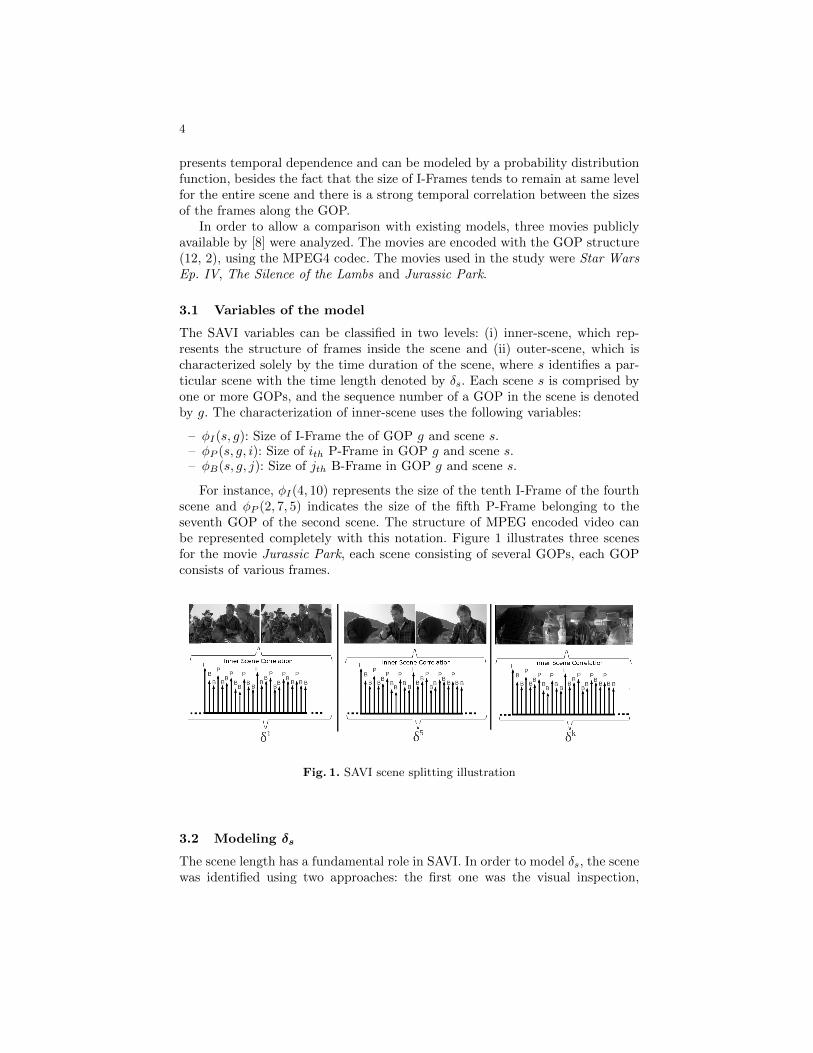
For instance, φI(4, 10) represents the size of the tenth I-Frame of the fourthscene and φP (2, 7, 5) indicates the size of the fifth P-Frame belonging to theseventh GOP of the second scene. The structure of MPEG encoded video canbe represented completely with this notation. Figure 1 illustrates three scenesfor the movie Jurassic Park, each scene consisting of several GOPs, each GOPconsists of various frames.

Fig. 1. SAVI scene splitting illustration

3.2 Modeling δs

The scene length has a fundamental role in SAVI. In order to model δs, the scenewas identified using two approaches: the first one was the visual inspection,

5

observing the time instant where there is a scene change. The procedure wasrepeated three times for each movie and calculating an average of observations.The second approach, as a complement, employs the algorithm proposed by [2],which suggests that a sudden change in the size of two successive I-Frames marksthe beginning of a new scene. When the variation of size of two consecutive I-Frames are greater than a threshold, respectively of T1 and T2, this indicates thebeginning of a new scene. Empirically by comparing the results of the algorithmwith the practical observations, the values of T1 and T2 were respectively set at15% and 20%, and the result was equivalent to the visual inspection.

After perform the scene identification, the autocorrelation function (ACF)of scene lengths was analyzed. Figure 2 (a) shows the empirical δs PDF forthe three movies under consideration and Figure 2 (b) shows the ACF for theJurassic Park. For all three movies, there is no significant temporal dependencebetween the scene lengths, i.e. the scene length is independent of previous scenes,as Figure 2 (b) illustrates. Thus, it is possible to characterize δs using a Log-normal PDF1. Figure 2 (c) shows the QQPlot graph comparing the theoreticalLognormal PDF with the empirical data. The QQPlot is a graphical goodness-of-fit test: if the two samples have the same distribution, the points should lieunder a diagonal line at 45o, represented by the solid line in the figure. Thepoints represent the quantiles observed in the video vs. same quantile of Log-normal theoretical PDF. The graph also shows the limits for a confidence levelof 95% (dashed lines). Table I shows the parameters of Lognormal PDF for themovies under study. The result of Kolmogorv Smirnov goodness-of-fit test (KS-test) is also shown, and the calculated p-value indicates that the null hypothesiscan not be rejected (occurs when p-value is greater than 0.05 [9]).

●●●●●●●●●●●●●●●●●●●●●●

●

●

●

●

●

●

●

●

●

●

●●●●●●●●●●●●●●●●

●●●●●●●●●●●●●●●●●●●●●●●●●●●●●●●●●●●●●●●●●●●●●●●●●●●●●●●●●●●●●●●●●●●●●●●●●●●●●●●●●●●●●●●●●●●●●●●●●●●●●●●●●●●●●●●●●●●●●●●●●●●●●●●●●●●●●●●●●●●●●●●●●●●●●●●●●●●●●●●●●●●●●●●●●●●●●●●●●●●●●●●●●●●●●●●●●●●●●●●●●●●●●●●

0 5 10 15 20 25 30

0.00

0.04

0.08

0.12

Scene Length (s)

PD

F

● Silence Of The LambsStar Wars IVJurassic Park I

0 100 300 500 700

0.0

0.2

0.4

0.6

0.8

1.0

Lag

AC

F

0 20 40 60 80

010

2030

4050

60

Lognormal PDF (s)

Sce

ne L

engt

h (s

)

●●●●●●●●●●●●●●●●●●●●●●●●●●●●●●●●●●●●●●●●●●●●●●●●●●●●●●●●●●●●●●●●●●●●●●●●●●●●●●●●●●●●●●●●●●●●●●●●●●●●●●●●●●●●●●●●●●●●●●●●●●●●●●●●●●●●●●●●●●●●●●●●●●●●●●●●●●●●●●●●●●●●●●●●●●●●●●●●●●●●●●●●●●●●●●●●●●●●●●●●●●●●●●●●●●●●●●●●●●●●●●●●●●●●●●●●●●●●●●●●●●●●●●●●●●●●●●●●●●●●●●●●●●●●●●●●●●●●●●●●●●●●●●●●●●●●●●●●●●●●●●●●●●●●●●●●●●●●●●●●●●●●●●●●●●●●●●●●●●●●●●●●●●●●●●●●●●●●●●●●●●●●●●●●●●●●●●●●●●●●●●●●●●●●●●●●●●●●●●●●●●●●●●●●●●●●●●●●●●●●●●●●●●●●●●●●●●●●●●●●●●●●●●●●●●●●●●●●●●●●●●●●●●●●●●●●●●●●●●●●●●●●●●●●●●●●●●●●●●●●●●●●●●●●●●●●●●●●●●●●●●●●●●●●●●●●●●●●●●●●●●●●●●●●●●●●●●●●●●●●●●●●●●●●●●●●●●●●●●●●●●●●●●●●●●●●●●●●●●●●●●●●●●●●●●●●●●●●●●●●●●●●●●●●●●●●●●●●●●●●●●●●●●●●●●●●●●●●●●●●●●●●

●●●●●●●●●●

●●●●●●●●●●

●●●●●●●●

●●●●●

● ● ●●

●

(a) (b) (c)

Fig. 2. Scene length: (a) empirical PDF for the three movies, (b) ACF of Jurassic Parkand (c) QQPlot of Jurassic Park

1 Probability density given by f(x) = 1

xσ√2πe−(lnx−µ)2/2σ2

, µ is the average and σ

the standard deviation of ln(x)

6

Table 1. Scene Length model

Title Probability Parameters K-S testDistribution (p-value)

Jurassic Park Lognormal µ = 2.013; σ = 0.793 0.36Star Wars Episode IV Lognormal µ = 1.749; σ = 0.710 0.40The Silence of the Lambs Lognormal µ = 1.640; σ = 0.779 0.66

3.3 Modeling φI(s, g)

The size of I-Frames was modeled by considering the movie split in scenes. Withina scene, the time series formed by the size of successive I-Frames depend on thefirst I-Frame of the scene. However, the first I-Frame of each scene, φI(s, 1), hasno time dependence with the I-Frames of previous scene. Thus, the approachtaken was to model φI(s, 1) and, from its value, to obtain the size of the otherI-Frames of the scene.

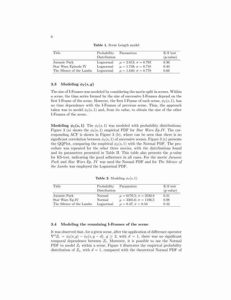
Modeling φI(s, 1) The φI(s, 1) was modeled with probability distributions.Figure 3 (a) shows the φI(s, 1) empirical PDF for Star Wars Ep.IV. The cor-responding ACF is shown in Figure 3 (b), where can be seen that there is nosignificant correlation between φI(s, 1) of successive scenes. Figure 3 (c) presentsthe QQPlot, comparing the empirical φI(s, 1) with the Normal PDF. The pro-cedure was repeated for the other three movies, with the distributions foundand its parameters presented in Table II. This table also presents the p-valuefor KS-test, indicating the good adherence in all cases. For the movie JurassicPark and Star Wars Ep. IV was used the Normal PDF and for The Silence ofthe Lambs was employed the Lognormal PDF.

Table 2. Modeling φI(s, 1)

Title Probability Parameters K-S testDistribution (p-value)

Jurassic Park Normal µ = 6170.5; σ = 2530.8 0.31Star Wars Ep.IV Normal µ = 3305.6; σ = 1106.5 0.98The Silence of the Lambs Lognormal µ = 8.47; σ = 0.53 0.42

3.4 Modeling the remaining I-Frames of the scene

It was observed that, for a given scene, after the application of difference operator∇dZt = φI(s, g) − φI(s, g − d), g ≥ 2, with d = 1, there was no significanttemporal dependence between Zt. Moreover, it is possible to use the NormalPDF to model Zt within a scene. Figure 4 illustrates the empirical probabilitydistribution of Zt, with d = 1, compared with the theoretical Normal PDF of

7

0 2000 4000 6000 8000

0.00

000

0.00

010

0.00

020

0.00

030

φI(s, 1)(bytes)

PD

F

0 100 200 300 400

0.0

0.2

0.4

0.6

0.8

1.0

Lag

AC

F

0 1000 3000 5000

2000

4000

6000

8000

Normal PDF (bytes)

φ I(s

, 1)(b

ytes

)

●●●●●●●●

●●●●●●●●●●●●●●●●●●

●●●●●●●●●●●●●●●●●●●

●●●●●●●●●●●●●●●●●●●●●●●●●●●●●●●

●●●●●●●●●●●●●●●●●●●●●●●●●●●●●●●●●●●●●●●●●●●●●●●●●●●●●●●●●●●●●●●●●●●●●●●●●●●●●●●●●●●●●●

●●●●●●●●●●●●●●●●●●●●●●●●●●●●●●●●●●●●●●●●●●●●●●●●●●●●●●●●●●●●

●●●●●●●●●●●●●●●●●●●●●●●●●●●●●●●●●●●●●●●●●●●●●●●

●●●●●●●●●●●●●●●●●●●●●●●●●●●●●●●●●●●●●●●●●●●●●●●●●●●

●●●●●●●●●●●●●●●●●●●●●●●●●●●●●●●●●●●●●●●●

●●●●●●●●●●●●●●●●●●●●●●●●●●●●●●

●●●●●●●●●●●●●●●●●●●●●●●●●●●●●●●●●●●●●●●●●●●●●●●●●●●

●●●●●●●●●●●●

●●●●●●●●

●

●

(a) (b) (c)

Fig. 3. φI(s, 1): (a) Empirical PDF (solid lines), compared with the Normal PDF(dotted lines), (b) ACF and (c) QQPlot for Star Wars Episode IV

four scenes of Jurassic Park. Table III shows the result of KS-test for thosescenes, where the p-value indicates the good similarity with the Normal PDF. Asimilar trend was observed in the other scenes of the movies under consideration.

Table 3. Modeling φI(s, g), g ≥ 2: four scenes of Jurassic Park

Scene Probability Parameters KS-testNumber Distribution (p-value)

59 Normal µsg = 7.7; σsg = 170 0.3267 Normal µsg = −5.1; σsg = 120 0.31131 Normal µsg = −2.1; σsg = 150 0.34208 Normal µsg = −6.7; σsg = 240 0.75

Thus, the remaining I-Frames of a scene may be obtained from φI(s, 1) usingEquation 1, as follows:

φI(s, g) = φI(s, g − 1) +N(0, σsg), g ≥ 2 (1)

where N(0, σsg) represents the standard normal distribution.

3.5 Modeling φP (s, g, i)

The modeling of φP (s, g, i) is an adaptation of the idea originally presented by[3]. It was observed that the size of the first P-Frame of the GOP are correlatedwith the size of I-Frame which starts the GOP. The correlation is given byEquation 2, as follows:

8

Fig. 4. Empirical PDF of the I-Frame size for several scenes of the movie Jurassic Park,after applying the ∇1 operator (dotted lines), compared with the Normal PDF (solidlines)

ρφI(s,g),φP (s,g,1) =(E[φI(s, g) · φP (s, g, 1)]−E[φI(s, g)] · E[φP (s, g, 1)])/√

(E[φI(s, g)2]− E2[φI(s, g)]·(E[φP (s, g, 1)]2)− E2[φP (s, g, 1)])

(2)

The correlation value ρ is in the range from -1 to 1. The most significantcorrelation occur with |ρ| = 1, and ρ = 0 indicates no correlation between thevariables. The movies under study were analyzed and the values obtained for ρare shown in Table IV. The result indicates that there is a significant correlationbetween the size of the I-Frame and the first P-Frame of GOP.

The size of remaining P-Frames of GOP may be obtained using Equation 3,where αP represents a random variable with Gamma PDF. Further details canbe obtained in [3].

φP (s, g, i) = φI(s, g) ·ρφI(s,g),φP (s,g,1) · σφP (s,g,1)

σφI(s,g)+ αP (3)

9

Table 4. Correlation between size of I, P and B-Frames of GOP

Title ρφI (s,g),φP (s,g,1) ρφP (s,g,1),φB(s,g,1)

Jurassic Park 0.7781 0.8629Star Wars Ep.IV 0.6155 0.7508The Silence of the Lambs 0.8887 0.9358

3.6 Modeling φB(s, g, j)

The modeling of φB(s, g, j) follows the same procedure performed for the P-Frame, however, regarding the size of the first P-Frame of the GOP insteadI-Frame. Thus, φB(s, g, j) can be obtained by changing I by P and B by Pin the Equation 3. The correlation between the φB(s, g, 1) and the φP (s, g, 1)should be established in the same way. The variable αB can also be modeledwith the Gamma PDF. Table IV shows the correlation between φP (s, g, 1) andφB(s, g, 1).

4 Generation of synthetic workload

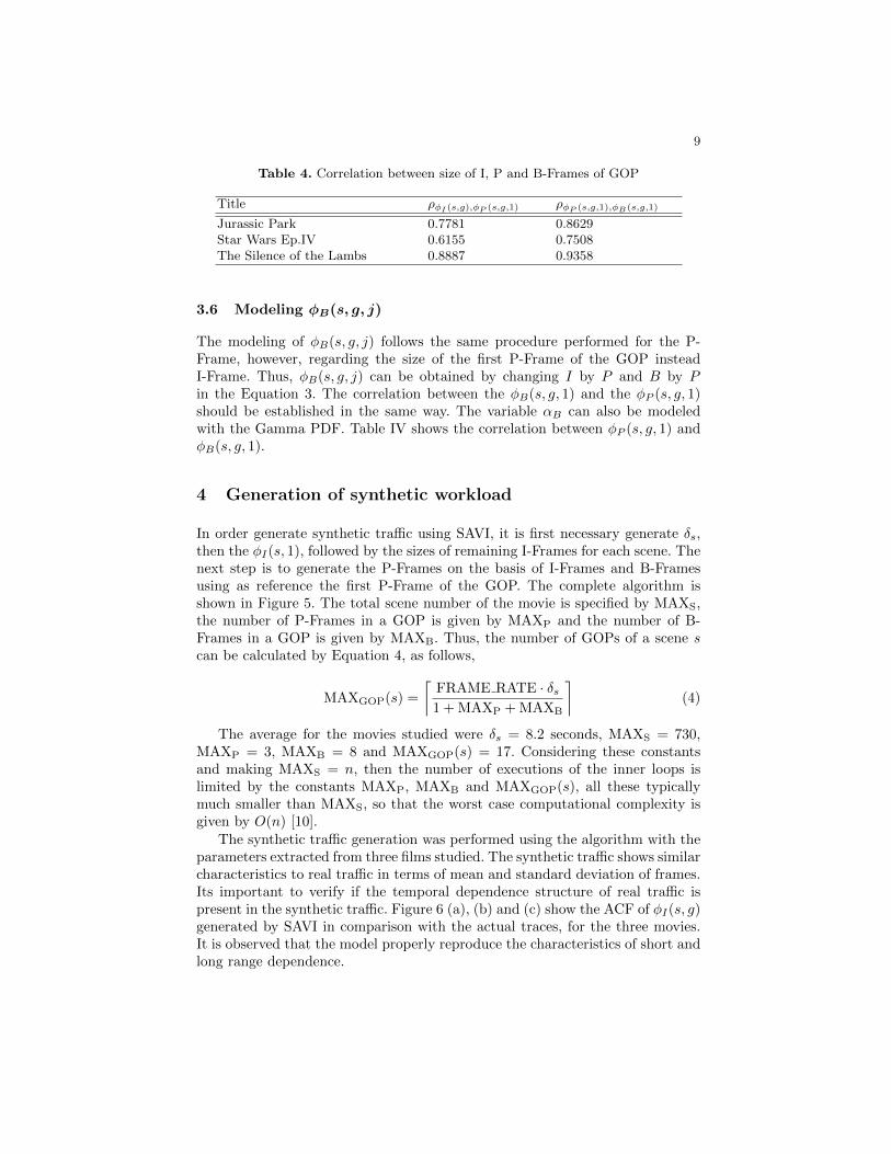
In order generate synthetic traffic using SAVI, it is first necessary generate δs,then the φI(s, 1), followed by the sizes of remaining I-Frames for each scene. Thenext step is to generate the P-Frames on the basis of I-Frames and B-Framesusing as reference the first P-Frame of the GOP. The complete algorithm isshown in Figure 5. The total scene number of the movie is specified by MAXS,the number of P-Frames in a GOP is given by MAXP and the number of B-Frames in a GOP is given by MAXB. Thus, the number of GOPs of a scene scan be calculated by Equation 4, as follows,

MAXGOP(s) =

⌈FRAME RATE · δs1 + MAXP + MAXB

⌉(4)

The average for the movies studied were δs = 8.2 seconds, MAXS = 730,MAXP = 3, MAXB = 8 and MAXGOP(s) = 17. Considering these constantsand making MAXS = n, then the number of executions of the inner loops islimited by the constants MAXP, MAXB and MAXGOP(s), all these typicallymuch smaller than MAXS, so that the worst case computational complexity isgiven by O(n) [10].

The synthetic traffic generation was performed using the algorithm with theparameters extracted from three films studied. The synthetic traffic shows similarcharacteristics to real traffic in terms of mean and standard deviation of frames.Its important to verify if the temporal dependence structure of real traffic ispresent in the synthetic traffic. Figure 6 (a), (b) and (c) show the ACF of φI(s, g)generated by SAVI in comparison with the actual traces, for the three movies.It is observed that the model properly reproduce the characteristics of short andlong range dependence.

10

for s← 1 to MAXS doGenerate δ(s);Generate φI(s, 1);Evaluate MAXGOP(s) (Equation 4)for g ← 2 to MAXGOP(s) do

Generate φI(s, g);Generate φP (s, g, 1);Generate φB(s, g, 1);for i← 2 to MAXP do

Generate φP (s, g, i);endfor j ← 2 to MAXB do

Generate φB(s, g, j);end

end

end

Fig. 5. SAVI algorithm for workload generation.

Fig. 6. ACF for φI(s, g) generated by SAVI compared with real traces for (a) StarWars Ep.IV , (b) The Silence of the Lambs and (c) Jurassic Park.

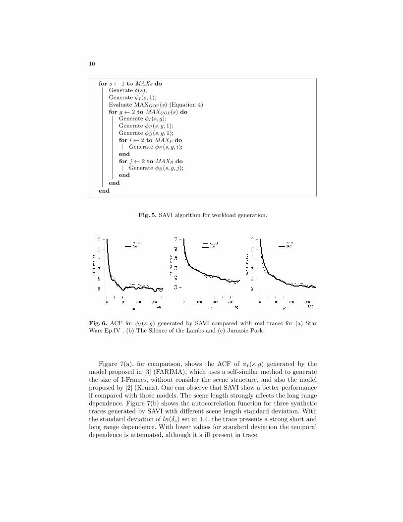
Figure 7(a), for comparison, shows the ACF of φI(s, g) generated by themodel proposed in [3] (FARIMA), which uses a self-similar method to generatethe size of I-Frames, without consider the scene structure, and also the modelproposed by [2] (Krunz). One can observe that SAVI show a better performanceif compared with those models. The scene length strongly affects the long rangedependence. Figure 7(b) shows the autocorrelation function for three synthetictraces generated by SAVI with different scene length standard deviation. Withthe standard deviation of ln(δs) set at 1.4, the trace presents a strong short andlong range dependence. With lower values for standard deviation the temporaldependence is attenuated, although it still present in trace.

11

Fig. 7. (a) ACF for φI(s, g) generated by SAVI for the movie The Silence of the Lambscompared with several models and (b) Autocorrelation function of three synthetictraces generated by SAVI with several scene length standard deviation.

5 Conclusions

In this article has been proposed a new model for MPEG workload generationusing the scene length as basis for generating the frame sizes. SAVI creates theframe sequence using a sum of random variables and is able to reproduce thetemporal dependence observed in real data properly. Furthermore, SAVI relatesthe random variables with the specific characteristics of the movie, providingan explanation on the meaning of each variable. The model also provides anexplanation on the causes of self similarity in video traffic.

The use of scene length allows to establish traffic patterns related with thischaracteristic. This is difficult to achieve with existing models, which depend onparameters that can not be related so explicitly with the observable character-istics of the movie. Additionally, SAVI presents low computational complexityif compared to most of the available methods for video workload generation. Asfuture work we are extending the analysis to other video traces.

References

1. Menasce, D.A., Almeida, V.A.F.: Capacity planning for Web performance. PrenticeHall (1998)

2. Krunz, M., Tripathi, S.K.: On the characterization of VBR MPEG streams. SIG-METRICS Performance Evaluation Rev. 25(1) (June 1997) 192–202

3. Dai, M., Zhang, Y., Loguinov, D.: A unified traffic model for MPEG-4 and H.264video traces. IEEE Transactions on Multimedia 11 (2009) 1010–1023

12

4. Manzoni, P., Cremonesi, P., Serazzi, G.: Workload models of VBR video traffic andtheir use in resource allocation policies. IEEE/ACM Transactions on Networking7(3) (1999) 387–397

5. ISO: MPEG-4 part 14: MP4 file format; ISO/IEC 14496-14:2003 (2003) Interna-tional Organization for Standardization.

6. Garrett, M.W., Willinger, W.: Analysis, modeling and generation of self-similar vbrvideo traffic. In: SIGCOMM ’94: Proceedings of the conference on Communicationsarchitectures, protocols and applications, New York, NY, USA, ACM Press (1994)269–280

7. Rose, O.: A Memory Markov Chain for VBR traffic with strong positive correla-tions. In: 24th International Teletraffic Congress (ITC 16), Edinburgh, GB (1999)827–836

8. Fitzek, F., Reisslein, M.: MPEG-4 and H.263 video traces for network performanceevaluation. IEEE Network 15(6) (November 2001) 40–54

9. Jain, R.: The art of computer systems performance analysis: techniques for ex-perimental design, measurement, simulation and modeling. John Wiley & Sons(1991)

10. Arora, S., Barak, B.: Computational Complexity: A Modern Approach. 1st edn.Cambridge University Press, New York, NY, USA (2009)