Brigham Young University Brigham Young University BYU ScholarsArchive BYU ScholarsArchive Theses and Dissertations 2011-03-11 Sawdust Pyrolysis and Petroleum Coke CO2 Gasification at High Sawdust Pyrolysis and Petroleum Coke CO2 Gasification at High Heating Rates Heating Rates Aaron D. Lewis Brigham Young University - Provo Follow this and additional works at: https://scholarsarchive.byu.edu/etd Part of the Chemical Engineering Commons BYU ScholarsArchive Citation BYU ScholarsArchive Citation Lewis, Aaron D., "Sawdust Pyrolysis and Petroleum Coke CO2 Gasification at High Heating Rates" (2011). Theses and Dissertations. 2498. https://scholarsarchive.byu.edu/etd/2498 This Thesis is brought to you for free and open access by BYU ScholarsArchive. It has been accepted for inclusion in Theses and Dissertations by an authorized administrator of BYU ScholarsArchive. For more information, please contact [email protected], [email protected].
Transcript
Brigham Young University Brigham Young University
BYU ScholarsArchive BYU ScholarsArchive
Theses and Dissertations
2011-03-11
Sawdust Pyrolysis and Petroleum Coke CO2 Gasification at High Sawdust Pyrolysis and Petroleum Coke CO2 Gasification at High
Heating Rates Heating Rates
Aaron D. Lewis Brigham Young University - Provo
Follow this and additional works at: https://scholarsarchive.byu.edu/etd
Part of the Chemical Engineering Commons
BYU ScholarsArchive Citation BYU ScholarsArchive Citation Lewis, Aaron D., "Sawdust Pyrolysis and Petroleum Coke CO2 Gasification at High Heating Rates" (2011). Theses and Dissertations. 2498. https://scholarsarchive.byu.edu/etd/2498
This Thesis is brought to you for free and open access by BYU ScholarsArchive. It has been accepted for inclusion in Theses and Dissertations by an authorized administrator of BYU ScholarsArchive. For more information, please contact [email protected], [email protected].
Clean and efficient electricity can be generated using an Integrated Gasification Combined Cycle (IGCC). Although IGCC is typically used with coal, it can also be used to gasify other carbonaceous species like biomass and petroleum coke. It is important to understand the pyrolysis and gasification of these species in order to design commercial gasifiers and also to determine optimal conditions for operation.
High heating-rate (105 K/s) pyrolysis experiments were performed with biomass
(sawdust) in BYU’s atmospheric flat-flame burner reactor at conditions ranging from 1163 to 1433 K with particle residence times ranging from 23 to 102 ms. Volatile yields and mass release of the sawdust were measured. The measured pyrolysis yields of sawdust are believed to be similar to those that would occur in an industrial entrained-flow gasifier since biomass pyrolysis yields depend heavily on heating rate and temperature. Sawdust pyrolysis was modeled using the Chemical Percolation Devolatilization model assuming that biomass pyrolysis occurs as a weighted average of its individual components (cellulose, hemicellulose, and lignin). Thermal cracking of tar into light gas was included using a first-order kinetic model.
The pyrolysis and CO2 gasification of petroleum coke was studied in a pressurized flat-
flame burner up to 15 atm for conditions where the peak temperature ranged from 1402 to 2139 K. The measured CO2 gasification kinetics are believed to be representative of those from an entrained-flow gasifier since they were measured in similar conditions of elevated pressure and high heating rates (105 K/s). This is in contrast to the gasification experiments commonly seen in the literature that have been carried out at atmospheric pressure and slow particle heating rates. The apparent first-order Arrhenius kinetic parameters for the CO2 gasification of petroleum coke were determined. From the experiments in this work, the ASTM volatiles value of petroleum coke appeared to be a good approximation of the mass release experienced during pyrolysis in all experiments performed from 1 to 15 atm. The reactivity of pet coke by CO2 gasification exhibited strong pressure dependence.
Figure F.2. HPFFB during temperature measurements ............................................................. 137
Figure F.3. View factors in the HPFFB ..................................................................................... 137
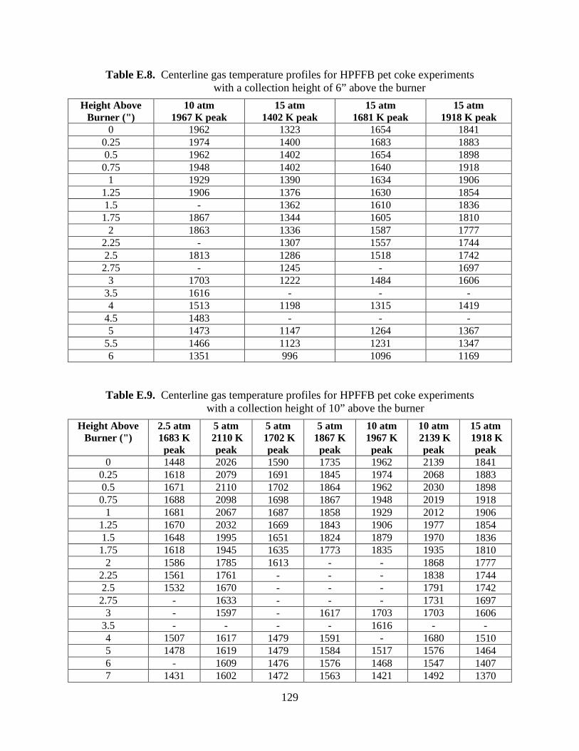
Figure G.1. Apparatus used to coat thermocouple beads with an alumina coating ................... 140
Figure G.2. Inside workings of the thermocouple bead coater .................................................. 141
Figure G.3. Experimental setup to test a thermocouple bead coating ....................................... 142
Figure H.1. Depiction of the forces on a single particle in the flat-flame burner reactors ........ 144
Figure H.2. Empirical fit of gas viscosity in the FFB and HPFFB ............................................ 146
Figure H.3. Experimental setup to measure particle velocities in the HPFFB. ......................... 151
Figure H.4. Two representative particle velocity profiles ......................................................... 152
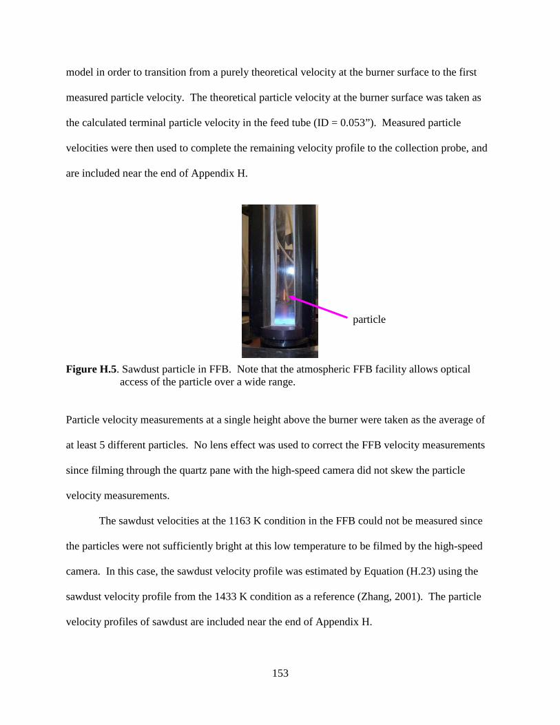
Figure H.5. Sawdust particle in FFB ......................................................................................... 153
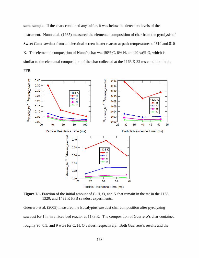
Figure I.1. Fraction of the initial amount of C, H, O, and N that remain in the sawdust tar ..... 163
Figure I.2. Atomic ratio of sawdust chars as a function of temperature .................................... 165
Figure I.3. Fraction of the initial amount of C, H, O, and N that remain in the sawdust char ... 165
xii
Figure I.4. Compositional progression as sawdust transforms into char ................................... 166
Figure K.1. Ratio of particle diameters of pyrolyzed pet coke char .......................................... 173
Figure K.2. Ratio of particle diameters of gasified pet coke char ............................................. 173
Figure L.1. Apparent density of pet coke chars from the 1, 2.5, and 5 atm conditions ............. 176
Figure L.2. Apparent density of pet coke chars from the 10 and 15 atm conditions ................. 176
Figure M.1. Tar yields of pet coke. ............................................................................................ 179
Figure N.1. Fraction of the initial amount of H that remained in the pet coke char .................. 183
Figure N.2. Fraction of the initial amount of N that remained in the pet coke char .................. 184
Figure N.3. Fraction of the initial amount of S that remained in the pet coke char
................... 184
xiv
NOMENCLATURE Variable Definition
a Acceleration
Ao Pre-exponential factor
A Cross-sectional area
C Concentration
Cd Drag coefficient
d Diameter
DAB Diffusion coefficient
E Activation energy
f Quadratic scaling factor used to predict HPFFB vp profiles
F Force
g Gravity (9.81 m/s2)
h Height above HPFFB burner (from burner surface up to max height at which vp,measured was taken)
h1 Height above HPFFB burner (from height L up to collection probe height) hc Heat transfer coefficient hm Mass transfer coefficient ΔHpry Heat of pyrolysis ΔHrxn Heat of reaction k Thermal conductivity krxn Reaction rate constant L maximum height above the burner at which vp,measured was taken in HPFFB
xv
m Mass
mratio Ratio of vp,measured to vp,theoretical at height L in HPFFB
MW Molecular weight
Nu Nusselt number
P Pressure
R Ideal gas constant
Re Reynolds number
Sh Sherwood number
t Time
T Temperature
v Velocity
v∞ Slip velocity
x Mass fraction
Δz Distance a particle traveled in a single time step εb Packing factor
εp Emissivity of particle
θ Blowing factor (correction of transfer coefficients during high mass transfer)
μ Dynamic viscosity
ν Mass of Carbon that reacts per mole of reactant
ρ Density
σ Stefan-Boltzmann constant
χ Chi factor (indication of effect of film diffusion)
1
1. Introduction
Developing countries and a growing world population place an ever-increasing demand
for energy. The solution to meeting the energy needs of the future will most likely come from a
combination of energy sources, two of which are biomass and petroleum coke. Biomass is a
sustainable fuel source which allows energy generation from biological material such as sawdust,
switchgrass, and yard clippings. Petroleum coke is a cheap and abundant by-product of oil
refining that mainly consists of carbon. One way that biomass and petroleum coke can be
transformed into useful energy is through gasification, which converts any carbon-containing
material to hydrogen and carbon monoxide through partial oxidation.
Although the chemical reactions governing gasification are well understood, there is still
much to be learned about gasification kinetics. This is especially true for the kinetics
representative of those experienced in a commercial gasifier. In this research, petroleum coke
was reacted with CO2 in a high-pressure flat-flame burner (HPFFB) up to 15 atm at high heating
rates. The measured CO2 gasification kinetics are believed to be representative of those from an
industrial setting since they were measured in similar conditions of elevated pressure and high
heating rates (~ 105 K/s). This is in contrast to the gasification experiments commonly seen in
literature that have been carried out at atmospheric pressure with slow particle heating rates. The
operating conditions under which gasification rates are measured are important since operating
conditions affect char structure and thus active surface area.
2
Pyrolysis precedes gasification or combustion and is the thermal decomposition of the
solid fuel into permanent gases, tar (condensable vapors), and char (solid residue) (Ranzi et al.,
2008). Studying pyrolysis is important since it precedes gasification and since the volatiles can
be up to 90 wt% for some types of biomass (Jenkins et al., 1998). In this research, the pyrolysis
yields of softwood sawdust were measured at varying reactor temperatures and particle residence
times using an atmospheric flat-flame burner. The measured pyrolysis yields of sawdust are
believed to be similar to those that would occur in an industrial entrained-flow combustor or
gasifier. This is because the relative yields of gas, tar, and char depend heavily on heating rate
and final temperature (Bridgwater, 1995), and the conditions in a flat-flame burner are
comparable to those used in industry. Sawdust pyrolysis was modeled using the Chemical
Percolation Devolatilization model (Fletcher et al., 1992) assuming that sawdust pyrolysis occurs
as a weighted average of its individual components (cellulose, hemicellulose, and lignin). Tar
cracking was taken into account by including 1st-order kinetics from literature.
3
2. Literature Review
This chapter gives background in several areas to better understand this research, and
includes a review of pertinent literature. Some of the covered topics include the composition of
biomass, primary and secondary pyrolysis, gasification, pet coke gasification experimental
studies, and modeling of biomass pyrolysis.
2.1 Composition of Biomass
Interest in converting biomass to fuels and chemicals was sparked in the 1970s due to the
oil crisis (Mohan et al., 2006). Although the heating value of biomass is less than that of coal,
biomass has the advantages of being renewable, CO2-neutral, and fairly abundant. Most biomass
research for energy use has focused on wood, but the major components of any biomass are the
same whether it be almond husks, corn stalks, wood, etc. All biomass is comprised mainly of
cellulose, hemicellulose, and lignin as seen in Figure 2.1. Biomass also contains a significant
amount of moisture, which can be as high as 30 to 40 wt%. Although present in lesser amounts,
biomass also contains organic extractives and inorganic minerals.
Cellulose provides support to the primary cell wall with its strong, crystalline structure,
making up about a third of all plant matter. Cellulose is made up of 5000 to 10,000 repeating
glucose units (Crawford, 1981). Hydrogen bonding between strands and between molecules
allows the cellulose network to lie flat (Mohan et al., 2006).
4
Figure 2.1. Representative chemical structures of cellulose, hemicellulose, and lignin (Internet1;
Internet2).
Hemicellulose is a group of carbohydrates that surround the cellulose fibers in plant cells,
and makes up about 25 wt% of dry wood (Rowell, 1984). Hemicellulose is composed of
polymerized monosaccharides such as glucose, mannose, galactose, xylose, and arbinose (Mohan
et al., 2006). Hemicellulose has a less rigid structure than cellulose, partially caused by
hemicellulose containing 30 to 65 times fewer repeating saccharide monomers than cellulose
(Soltes and Elder, 1981).
Lignin is found mostly between plant cell walls and makes up about 20 wt% of wood
(Bridgwater, 2004). Although lignin lacks an exact structure, it is characterized by a branched,
three-dimensional network containing many ether bonds (Mohan et al., 2006). Lignin has a very
stable aromatic structure, slightly resembling that of a low-rank coal.
2.2 Petroleum Coke
Petroleum coke, or pet coke, is a by-product from oil refining. It results from the Coker
process, which heats heavy ‘bottom-of-the-barrel’ oil until it cracks into more valuable gasoline
components. Pet coke has a lower amount of ash, moisture, and volatiles when compared to coal
(Yoon et al., 2007). Some of the advantages of pet coke are its cheap cost and high calorific
value, although it has the drawbacks of higher sulfur and vanadium contents (Yoon et al., 2007).
5
Pet coke is increasingly used in gasifiers since its high sulfur content introduces environmental
complications if combusted.
2.3 Background on Thermal Conversion
Combustion and gasification are commonly used to thermally convert both biomass and
pet coke into useable energy. Although this research focuses on gasification, some discussion of
combustion is given here due to the similarities of these processes, and to emphasize that
pyrolysis research is important for both gasification and combustion. The first step that a particle
passes through in either combustion or gasification is evaporation of any moisture from the
particle. At higher temperatures, pyrolysis occurs, which means that the particle thermally
decomposes into permanent gases, condensable vapors (tar), and solid residue (char) (Ranzi et
al., 2008). Lastly, the primary pyrolysis products are either totally or partially oxidized
depending on whether the process is combustion or gasification, respectively. Combustion and
gasification mainly refer to the O2-char and CO2-char/H2O-char heterogeneous reactions,
respectively. Evaporation and pyrolysis are common to both combustion and gasification.
2.4 Primary Pyrolysis
Primary pyrolysis is defined as the initial thermal decomposition into gas, tar, and char
upon heating, without secondary reactions in the gas phase. Pyrolysis is sometimes referred to as
devolatilization. These terms will be used synonymously in this thesis, even though the technical
difference between the two is whether or not the thermal decomposition of the particle takes
place in the absence (pyrolysis) or presence (devolatilization) of oxygen. Typical primary
6
pyrolysis yields of biomass and pet coke can be up to 90 and 13 wt%, respectively (Jenkins et al.,
1998; Milenkova et al., 2003).
Studying pyrolysis is important since it precedes combustion or gasification, although
pyrolysis can also be a stand-alone process. It is important in modeling to know when
devolatilization has finished and also the relative amounts of the devolatilization products (i.e.,
gas, tar, and char).
2.5 Secondary Pyrolysis
Secondary pyrolysis refers to processes such as cracking, polymerization, condensation,
or carbon deposition that result from the reaction of the primary pyrolysis products at high
temperatures and sufficiently long residence times (Smoot and Smith, 1985). These reactions
occur homogeneously in the gas phase and heterogeneously at the surface of the solid fuel or
char particles (Wurzenberger et al., 2002). Generally speaking, secondary pyrolysis receives
much less research attention than primary pyrolysis. However, secondary reactions have a very
important influence on biomass product distribution and usability. The secondary pyrolysis of
biomass will be addressed in this thesis.
It is necessary to understand how secondary pyrolysis reactions affect product utilization
of biomass, especially wood. Thermal cracking of tar into light gas is a very important
secondary reaction of wood due to the effect of this reaction on the product distribution of
pyrolysis yields (i.e., gas, tar, and char) at relatively low temperatures. Although tar yields can
be as high as 75 wt% following the primary pyrolysis of wood, tar cracking can cause light gas
to be the major product of pyrolysis provided a sufficiently hot reactor temperature (Bridgwater,
2004). The tar-cracking reaction results in a gas yield that increases proportionately to the
7
destruction of tar. If bio-oil is the desired product from the thermochemical conversion of wood,
then high liquid yields are desirable and the objective is to prevent any secondary reactions from
occurring. In most other thermochemical processes, even low tar yields can cause problems by
fouling and corroding equipment, causing damage to motors and turbines, lowering catalyst
efficiency, and condensing in transfer lines (Vassilatos et al., 1992; Brage et al., 1996; Baumlin
et al., 2005). No matter which thermochemical process is used to convert wood, it is important
to know information about the thermal stability of pyrolysis tar since it can provide useful
information about process design and operating conditions.
There is much literature that indicates wood tar begins to thermally crack into light gas
near 500 °C. Scott et al. (1988) support that it is unlikely that a wood particle can still be in the
primary pyrolysis phase at any temperature above 500 °C and that secondary reactions must
occur above this temperature. Other researchers have studied the conditions at which maximum
tar yields occur for use in making bio-oil from wood, and have concluded that these conditions
involve short residence times with high heating rates at a maximum temperature near 500 °C
(Scott and Piskorz, 1982, 1984; Bridgwater, 2003; Higman and Burgt, 2003; Li et al., 2004;
Kang et al., 2006; Mohan et al., 2006; Zhang et al., 2007).
Figure 2.2. Silver birch tar yields from a fluidized bed reactor (Stiles and Kandiyoti, 1989).
8
Plots in literature such as the one shown in Figure 2.2 suggest that tar yields from wood pyrolysis
pass through a maximum near 500 °C, and then decline at higher temperatures due to secondary
tar-cracking reactions. Exposing wood tar to high temperatures at long residence times causes
most of the tar to crack into light gas.
2.6 Biomass Pyrolysis Modeling
Pyrolysis reactions are extremely complex and result in a large number of intermediates.
Since developing an exact reaction mechanism for each species would be extremely challenging,
pyrolysis models simplify things by considering only the most important kinetics. These models
are incorporated into large simulation models using commercial CFD packages, such as
FLUENT, that aid in the design of industrial equipment by solving mass, momentum, and energy
balances.
Prakash and Karunanithi (2008) wrote a review concerning the many biomass pyrolysis
models available in literature. Di Blasi (2008) also authored an excellent review regarding the
modeling of wood pyrolysis. Although many simple models have already been developed,
additional research is needed since it would be beneficial to have a more generalized biomass
pyrolysis model. Pyrolysis rate constants are available in literature, but they are often specific to
a certain type of biomass in a particular reactor.
A more universal method of modeling biomass pyrolysis is representing biomass
pyrolysis as a sum of its main components, namely cellulose, hemicellulose, and lignin
(Koufopanos et al., 1989; Raveendran et al., 1996; Miller and Bellan, 1997; Pond et al., 2003).
This method has successfully predicted primary pyrolysis yields (gas, tar, char) of biomass, but
begins to fail when the parent material has a high ash content (Caballero et al., 1996; Biagini et
9
al., 2006). Couhert et al. (2009) found that the modeling the pyrolysis of biomass as the sum of
its components also fails when trying to predict individual gas species. Nevertheless,
representing biomass pyrolysis as a weighted average of its components is useful to predict yield
distribution between light gas, tar, and char.
Several researchers have modeled biomass pyrolysis using the additivity law combined
with the Chemical Percolation Devolatilization (CPD) model, which was originally developed to
model the devolatilization yields of coal (Fletcher et al., 1992). The CPD model uses a
description of coal structure, and models the rate of bridge breaking since coal has a chemical
makeup of aromatic clusters connected by labile bridges. To use the CPD model for biomass,
kinetic and structural parameters for cellulose, hemicellulose, and lignin must be determined. A
weighted average of the pyrolysis yields of each component is then needed to obtain overall gas
and tar yields. This approach of modeling biomass is used in this thesis to predict sawdust
devolatilization.
Sheng and Azevedo (2002) reported kinetic and structural CPD parameters for cellulose,
hemicellulose, and lignin based on a data fit of experiments in the literature. Their results do not
take into account secondary reactions of tar cracking thermally into light gas. Although Sheng
and Azevedo compared their model successfully with the pyrolysis yields of lignin, sawdust, and
sugar cane bagasse, their results were not reproducible. However, they did provide very useful
correlations to predict the fraction of cellulose and lignin of a particular biomass sample based
on ultimate and proximate analyses.
Vizzini et al. (2008) provide CPD parameters for the three biomass components, but also
included coefficients for the vapor pressure correlation for cellulose and hemicellulose that were
different than the original CPD model. Vizzini’s model also treated secondary tar cracking using
10
1st-order separate kinetics for cellulose, hemicellulose, and lignin. Lastly, their model used a
population balance of side chains to differentiate between the side chains that leave the particle
in the tar and ones that remain in the metaplast.
Pond et al. (2003) also developed kinetic and structural parameters for cellulose,
hemicellulose, and lignin for use in the CPD model. Their parameters allowed a satisfactory
prediction of volatile yields from black liquor, cellulose, and lignin. Pond’s parameters enabled
a prediction of volatile yields from primary pyrolysis since modeling secondary tar-cracking
reactions were not attempted.
Most modeling of biomass pyrolysis in literature is specific to a particular type of
biomass in a unique reactor. There is a lack of information on a generalized model of biomass
pyrolysis that can handle different types of biomass and that includes thermal cracking of tar.
This project will fill this gap in literature by presenting a model that can predict biomass
pyrolysis yields as a function of biomass composition, pressure, heating rate, time, and
temperature. Pyrolysis experiments of wood in a flat-flame burner will help evaluate the
pyrolysis model, and will provide realistic pyrolysis yields of a biomass in conditions similar to a
commercial entrained-flow reactor.
2.7 Gasification
Gasification is the process by which any carbonaceous species can be converted into a
gaseous fuel called synthesis gas through partial oxidation. This process is preceded by
pyrolysis and usually takes place commercially at 900-1500 °C and 25-40 bar (Higman and
Burgt, 2003). Gasification is carried out at these high temperatures and pressures in order to
speed along the relatively slow gasification kinetics. In a typical gasifier, roughly 20% of the
11
oxygen needed for stoichiometric combustion is provided (Smoot, 1993). The oxygen reacts
with only a fraction of the available carbon, and is entirely consumed in about 10 ms (Batchelder
et al., 1953). Although oxygen is present for only a short time in a gasifier, it is important since
the exothermic combustion reaction provides the heat that drives the endothermic gasification
reactions. These gasification reactions consume the remaining carbon through the reaction of the
char with common gasifying agents like CO2 and steam. These gases react with the char through
dissociative chemisorption onto the carbon surface (Essenhigh, 1981). As long as the
gasification reactions are not controlled by film diffusion, the internal surface area of the char
plays an important role since it provides many more reacting sites than are available on the
external char surface area.
The simplified global reactions that are important in a gasifier are listed in Table 2.1.
Table 2.1. Major global reactions of carbon combustion and gasification
∆Hrxn° (kJ/mol)
(Higman and Burgt, 2003)
Relative Rate at 1073 K and 0.1 atm (Walker et al., 1959)
C + O2 CO2 - 394 105 R2.1 C + H2O CO + H2 + 131 3 R2.2
C + CO2 2CO + 172 1 R2.3 C + 2H2 CH4 - 75 0.003 R2.4
This table also contains the relative rates of the global reactions from a review by Walker et al.
(1959). These rates have been normalized by surface area and come from the reactions of
various carbons with O2, H2O, CO2, and H2. The sources of carbon from which the relative rates
were calculated in Table 2.1 are coal char, graphite plates, graphitized carbon rods, electrode
carbon, and carbon black. The char combustion reaction (R2.1 of Table 2.1) is about 105 times
faster than the gasification reactions (R2.2 and R2.3) at 1073 K and 0.1 atm (Walker et al.,
12
1959). The gasification reaction with steam (R2.2) is about three times faster than the
gasification reaction with CO2 (R2.3) at the aforementioned conditions. The hydrogenation
reaction (R2.4) is several orders of magnitude slower than the gasification reactions and is
usually ignored in gasification studies (Smith et al., 1994). Note also that the combustion and
hydrogenation reactions (R2.1 and R2.4) are exothermic, while the main gasification reactions
(R2.2 and R2.3) are endothermic.
Although the gasification reactions and their thermodynamics are understood fairly well,
there is still much room for improvement in predicting gasification kinetics, especially for
industrial-like conditions. Modeling this heterogeneous reaction can become complicated very
quickly when considering all the influencing factors. Some of these include diffusion of
reactants, reactions with both H2O and CO2, particle size effects, pore diffusion, char ash
content, temperature and pressure variations, and changes in surface area (Smoot and Smith,
Si,particle, xSi,char, and xSi,ash are the mass fractions of silicon in the initial particle, char, and
ash, respectively. Using Equation (4.4), expressions for mchar and mash are determined in terms of
m0particle and substituted into Equation (4.1). The expression is then divided by m0
particle and
yields:
% mass release (daf) = 1001
1
,
,0
,
,0
⋅
−
−
ashSi
particleSi
charSi
particleSi
xx
xx
(4.5)
which allows mass release to be calculated from the mass fractions of silicon in the initial
particle, char, and ash.
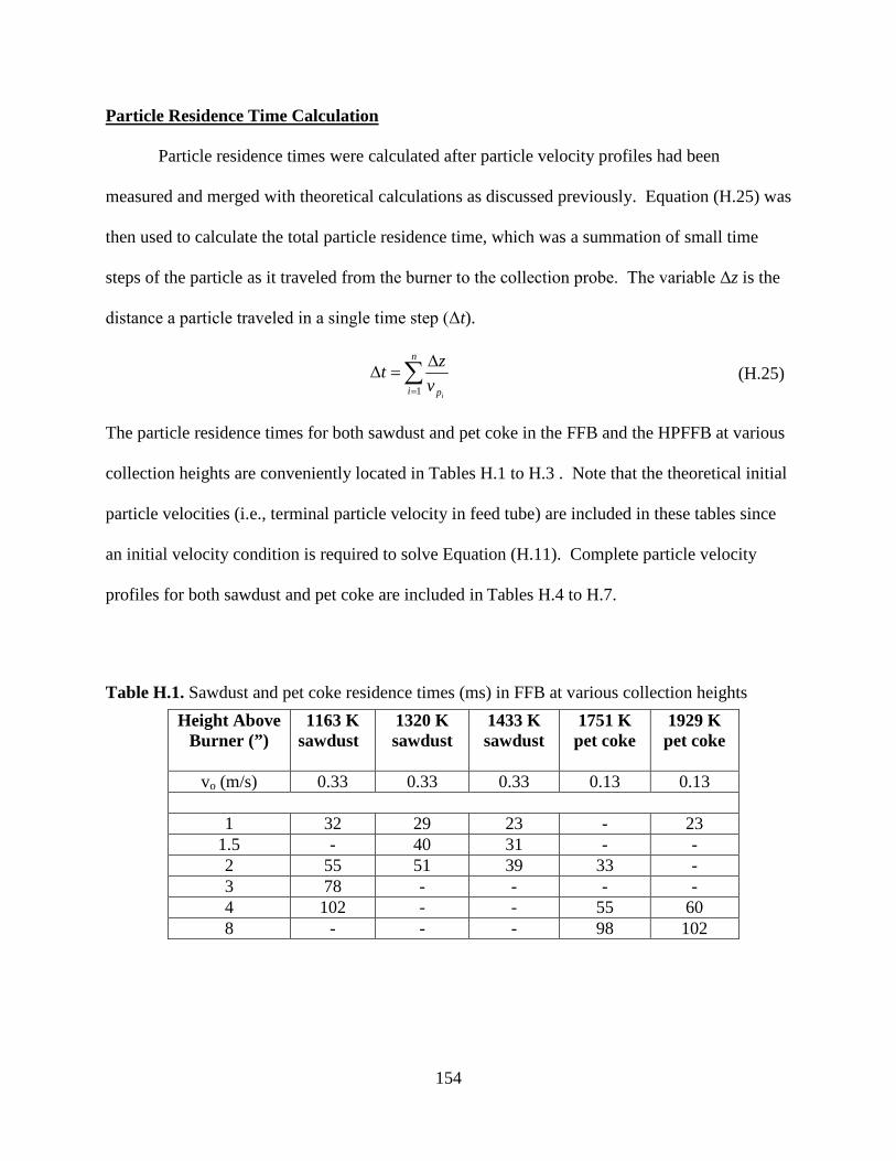
4.7 Determination of Particle Residence Times
It is very important to know the reaction time of a particle when determining particle kinetics.
The particle reaction time in this thesis was taken as the time it took a particle to travel from the
burner surface to the collection probe. A high-speed camera (Kodak EktaPro) was used to
measure sawdust and pet coke velocities in the FFB and the HPFFB. The total particle residence
time was then calculated using Equation (4.6) since the traveled particle distance was known as
well as the particle velocity. This equation was a summation of small time steps of the particle
as it traveled from the burner to the collection probe. The variable Δz is the distance a particle
traveled in a single time step (Δt). Additional details about measuring particle velocities and
calculating particle residence times are included in Appendix H.
∑=
∆=∆
n
i piv
zt1
(4.6)
26
27
5. Sawdust Pyrolysis Experiments and Modeling
High-temperature pyrolysis experiments were conducted on a single softwood sawdust in
an atmospheric flat-flame burner (FFB). This chapter focuses on the experimental results and
addresses mass release, volatile yields, char and tar elemental composition, and char structure.
Sawdust devolatilization modeling efforts using the CPD model are also discussed. Finely-
ground sawdust was used even though bigger biomass particles are typically used in industry.
The results can be used to predict upper bounds on total volatile yields in larger-scale equipment.
5.1 Sawdust Experimental Conditions at Atmospheric Pressure
Sawdust was dried at 107 °C for a minimum of 1 hour before use. Sawdust experiments
in the FFB were very time consuming due to the low ash content of the sawdust as well as
frequent clogging problems in the feeder tube. The low ash content of the sawdust affects the
amount of char required to perform an accurate ash test, which enabled the calculation of mass
release by ash tracer (see Section 4.6.1). A slightly larger feed tube could have helped resolve
this issue, but the tube’s inner diameter was fixed with a maximum near 0.053”. The average
sawdust char collected in a given week was ~ 400 mg. Sawdust was fed to the atmospheric flat-
flame burner (FFB) at a rate around 0.50 g/hr. Trying to increase the feed rate any further led to
more frequent clogging problems.
28
Sawdust pyrolysis experiments were performed at atmospheric pressure in the FFB at
peak temperatures of 1163, 1320, and 1433 K at three or four residence times per temperature. A
CO flame was used for the experiments, although some hydrogen was added for flame stability.
Figure 5.1 shows the centerline gas temperature profiles from these experiments, which have
been corrected for radiation losses from the thermocouple bead (see Appendix F). A table of
these measured temperatures is included in Table E.5 in the appendix. Table E.1 in the appendix
contains the gas conditions for the sawdust pyrolysis experiments.
Figure 5.1. Centerline temperature profiles from sawdust pyrolysis experiments using FFB.
5.2 Sawdust Pyrolysis Mass Release
Figure 5.2 shows the daf mass release data from the FFB sawdust pyrolysis experiments
at atmospheric pressure. The sawdust reached complete pyrolysis near 95 wt% daf at each of the
three residence times at both 1320 K and 1433 K, but not at the earliest residence time at 1163 K.
The particle residence time was simply not long enough at this low-temperature condition for the
sawdust to reach full pyrolysis before it entered the collection probe. The higher temperatures
29
allowed the sawdust to reach complete pyrolysis quicker, but did not affect mass release. The
mass release data in Figure 5.2 calculated by ash tracer (see Section 4.6.1) are summarized in
Table A.1 in the appendix. The mass release calculated by mass balance (using weight of char
collected and weight of raw sawdust fed) and ash tracer agreed within 5% at every condition,
except the 1163 K 32 ms case which had an 11% discrepancy. The mass release observed from
the sawdust FFB devolatilization experiments exceeded the ASTM volatiles value by 12% (see
Table 4.2).
Figure 5.2. Mass release of FFB sawdust pyrolysis experiments at atmospheric pressure at peak temperatures from 1163 to 1433 K.
5.3 Sawdust Pyrolysis Yields
Tar and gas yields from the sawdust atmospheric experiments appear in Figures 5.3 and
5.4. The tar yields were calculated based on the mass that collected on the water-cooled
micropore filters in the FFB collection system.
Note that the gas yields in Figure 5.4 were determined by difference, i.e., (100% – char
yield% – tar yield% – ash%). The yields in both Figures 5.3 and 5.4 were calculated on a basis
30
of dry ash-free sawdust fed. The reported yields were based on a mass balance (i.e., tar yield =
weight of collected tar/weight of daf sawdust fed), and are reported in Table A.3.
Figure 5.3. Tar yields from sawdust pyrolysis experiments in the FFB.
The high temperatures in the FFB resulted in very low tar yields, especially considering that
sawdust tar yields can be as high as 75 wt% at certain conditions (Bridgwater, 2003). Thermal
cracking of tar into light gas caused the low tar yields. Cracking becomes important above 800 K
(Scott et al., 1988) for biomass tars. Corresponding elemental compositions are given in
Appendix I.
Figure 5.4. Gas yields from sawdust pyrolysis experiments in the FFB.
31
It is interesting to note that the tar yields from the sawdust pyrolysis experiments level off
near 1.5 wt% at each of the 3 temperature conditions in the FFB. It is suggested in the literature
that there exists a small fraction of biomass tar that is or becomes refractory (Antal, 1983; Rath
and Staudinger, 2001; Bridgwater, 2003; Di Blasi, 2008). Other researchers have shown that
hotter reactor temperatures result in an increased fraction of aromatic compounds and condensed
ring structures in the biomass tar (Stiles and Kandiyoti, 1989; Zhang et al., 2007). The sawdust
tar collected in the FFB experiments was such a refractory tar since the hotter temperatures did
not lower the tar yield.
The interested reader is directed to Appendix I for a discussion on the elemental
composition of the sawdust tar and char collected from the FFB experiments.
5.4 SEM Images of Sawdust Char
SEM images of sawdust char collected at 1163, 1320, and 1433 K from BYU’s FFB are
shown in Figures 5.5 to 5.7. These images were taken at BYU using a FEI XL30 ESEM with a
FEG emitter. Note that some of the images were taken at 100x magnification whereas others
were taken at a magnification of 200x. Each of these figures shows the progression of char at
increasing particle residence times at a single temperature.
The amount of char-like particles qualitatively increased with increasing particle
residence time at each temperature condition, where char-like particles refer to those rounder
particles that appear to have passed through a plastic stage. The fraction of wood-like particles
qualitatively decreased with increasing residence time at each FFB condition, where wood-like
particles refer to those particles with higher aspect ratios that resemble the raw sawdust (see
Figure 4.1). The sawdust particles transformed to more sphere-like particles as they progressed
32
to char. From a qualitative analysis, the ratio of char-like particles to wood-like particles
appeared higher for the 1320 K condition than for the 1163 K condition at the ~50 ms particle
residence time (see Figure 5.5 & Figure 5.6). This indicates that the sawdust transforms to char
more quickly at higher temperatures. Further evidence of this can be seen by comparing the
1320 K and 1433 K chars at the ~40 ms particle residence time (see Figure 5.6 & Figure 5.7).
32 ms32 ms 55 ms55 ms
78 ms78 ms 102 ms102 ms
Figure 5.5. SEM images of sawdust char obtained in the FFB at the 1163 K condition. Note that the SEM image of the char collected at 102 ms is at a different magnification than the rest of the SEM images of char in this figure.
Mass release is essentially complete for all of these chars, except for the 1163 K 32 ms sawdust
char (see Figure 5.2). This suggests that the shape of the sawdust continues to change even after
33
mass release is complete. Longer particle residence times would likely result in a higher fraction
of rounded particles, but would not significantly affect mass release.
Figure 5.8 shows a close-up of sawdust char collected from the 1433 K FFB condition
that was collected after 39 ms. Similar to the results found by Cetin et al. (2004), the original
structure does not exist after devolatilization due to melting of the cell structure and plastic
transformations. Just as is observed in Figure 5.8, both Zhang et al. (2006) and Dupont et al.
(2008) pyrolyzed sawdust in drop-tube reactors and noticed that the sawdust char was spherical
with many voids and pores.
29 ms29 ms 40 ms40 ms
51 ms51 ms
Figure 5.6. SEM images of sawdust char obtained in the FFB at the 1320 K condition.
34
These morphological changes that occured to the sawdust are likely only characteristic of chars
pyrolyzed at high heating rates since Cetin et al. (2004) did not observe any major structural
changes of sawdust pyrolyzed at a low heating rate of 20 K/s.
23 ms23 ms 31 ms31 ms
39 ms39 ms
Figure 5.7. SEM images of sawdust char obtained in the FFB at the 1433 K condition. The fact that sawdust particles turn spherical after pyrolysis at high heating rates means that
combustion or gasification of sawdust can be modeled assuming spherical particles.
35
Figure 5.8. Close-up view of sawdust char collected from 1433 K 39 ms in the FFB.
5.5 Sawdust Pyrolysis Modeling
The biomass devolatilization modeling efforts in this thesis stem from the work of Pond
et al. (2003) and other researchers (Sricharoenchaikul, 2001; Sheng and Azevedo, 2002). Pond
et al. proposed structural and kinetic parameters for the biomass components of cellulose,
hemicellulose, and lignin for use in the Chemical Percolation Devolatilization (CPD) model
(Fletcher et al., 1992), which was originally developed to predict coal devolatilization yields as a
function of time, temperature, pressure, and heating rate. The CPD model assumes a base
structural unit of biomass, and predicts pyrolysis yields based on how the initial structure breaks
apart at high temperatures. Pond’s proposed CPD parameters for biomass modeling are shown
in Tables 5.2 and 5.3. The five structural parameters in the CPD model are molecular weight of
the cluster (MW1), molecular weight of side chains (Mδ), initial fraction of intact bridges (po),
coordination number (σ+1), and initial fraction of char bridges (co). The definitions of the
kinetic parameters of the CPD model are summarized in Table 5.1.
Pond et al. (2003) compared predicted primary pyrolysis yields (i.e., char, tar, and light
gas) with experimental pyrolysis yields of cellulose, lignin, and black liquor. The work of this
thesis evaluates the effectiveness of the model at predicting measured sawdust pyrolysis yields.
36
A tar-cracking model was added to account for the secondary reaction of tar thermally cracking
into light gas.
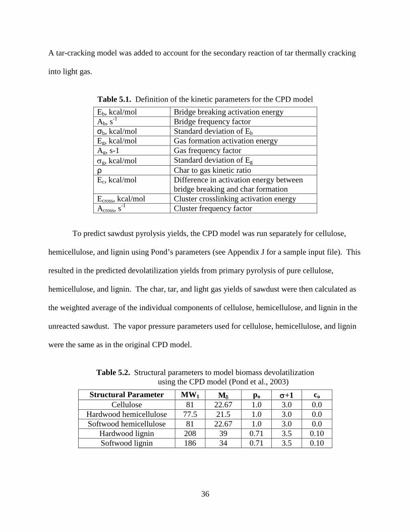
Table 5.1. Definition of the kinetic parameters for the CPD model
Eb, kcal/mol Bridge breaking activation energy Ab, s-1 Bridge frequency factor σb, kcal/mol Standard deviation of Eb Eg, kcal/mol Gas formation activation energy Ag, s-1 Gas frequency factor σg, kcal/mol Standard deviation of Eg ρ Char to gas kinetic ratio Ec, kcal/mol Difference in activation energy between
bridge breaking and char formation Ecross, kcal/mol Cluster crosslinking activation energy Across, s-1 Cluster frequency factor
To predict sawdust pyrolysis yields, the CPD model was run separately for cellulose,
hemicellulose, and lignin using Pond’s parameters (see Appendix J for a sample input file). This
resulted in the predicted devolatilization yields from primary pyrolysis of pure cellulose,
hemicellulose, and lignin. The char, tar, and light gas yields of sawdust were then calculated as
the weighted average of the individual components of cellulose, hemicellulose, and lignin in the
unreacted sawdust. The vapor pressure parameters used for cellulose, hemicellulose, and lignin
were the same as in the original CPD model.
Table 5.2. Structural parameters to model biomass devolatilization
using the CPD model (Pond et al., 2003)
Structural Parameter MW1 Mδ po σ+1 co Cellulose 81 22.67 1.0 3.0 0.0
Vizzini’s (2008) kinetics were applied to the primary pyrolysis tar yields of cellulose,
hemicellulose, and lignin from the CPD model. The resulting tar yields were then combined by
the weighted average of cellulose, hemicellulose, and lignin. The thermally-cracked tar yields
were then added to the weighted gas yields. The weighted CPD char yield remained unchanged
when considering secondary tar-cracking reactions. The use of Vizzini’s tar-cracking model
maintained a very generalized biomass devolatilization model since both the primary and
secondary pyrolysis yields were predicted based on a weighted average of the individual biomass
components of cellulose, hemicellulose, and lignin. It is also possible to use tar-cracking
kinetics specific to the biomass of interest by applying particular tar-cracking kinetics to the
primary pyrolysis tar yields of the CPD model. For example, Fagbemi et al. (2001) proposed a
model and reported kinetic parameters to predict tar-cracking specific to sawdust.
39
Figure 5.9 shows a comparison between predicted yields from sawdust devolatilization
and experimental yields obtained at BYU in the FFB at atmospheric pressure at conditions with
peak temperatures of 1163, 1320, and 1433 K.
Figure 5.9. Comparison of sawdust yields between the CPD model’s prediction with Vizzini’s tar-cracking kinetics and BYU’s FFB experiments at atmospheric pressure and peak temperatures of 1163, 1320, and 1433 K.
The maximum initial particle heating rates for the three temperature conditions were 2.5x10⁵,
3.8x10⁵, and 7.2x10⁵ K/s, respectively. The fractions used for the cellulose, lignin, and
hemicellulose components were 0.461, 0.287, and 0.252.
The predicted sawdust yields in Figure 5.9 were performed using the CPD model with
Pond’s (2003) parameters combined with Vizzini’s (2008) secondary tar-cracking model. The
char prediction matches very well with experimental values in every case. The predictions using
the simple 1st-order tar-cracking kinetics of Vizzini et al. (2008) matched the measured sawdust
40
pyrolysis yields in the FFB within 4.3 daf wt% upon complete pyrolysis at 1163, 1320, and 1433
K. There is room for improvement in the modeling of the shorter residence times of the 1163 K
case (see Figure 5.9). The agreement between model and experimental gas and tar yields was
improved in this case after tar-cracking kinetics specific to sawdust were used (see Figure 5.10).
In Figure 5.10, the sawdust tar-cracking model of Fagbemi et al. (2001) was used. The values of
the pre-exponential factor and activation energy were 4.28x10⁶ s-1 and 107.5 kJ/mole,
respectively.
Figure 5.10. Comparison of sawdust yields between the CPD model’s prediction with Fagbemi’s (2001) tar-cracking kinetics and BYU’s FFB experiments at 1163 K and atmospheric pressure.
Figure 5.11 is included for reference to show the predictions of the CPD model using
Pond’s kinetic parameters without
Figure 5.11
including a secondary tar-cracking model for the FFB 1163 K
case. The modeled yields in the figure are the predicted sawdust yields resulting solely from
primary pyrolysis. Note that in the predicted primary tar yield matches the measured
gas yield, and vice versa. This figure clearly illustrates the need for a tar-cracking model since
the measured tar and gas yields were so different from their predicted values.
41
Figure 5.11. Comparison of sawdust yields between the CPD model’s prediction without Vizzini’s tar-cracking kinetics and BYU’s FFB experiments at 1163 K and atmospheric pressure.
5.5.1 Comparison of CPD Model with Experiments from Literature
Sawdust pyrolysis data were found in the literature in order to further evaluate how well
the CPD model predicts sawdust devolatilization using Pond’s (2003) kinetic parameters with
Vizzini’s (2008) secondary tar-cracking kinetics. The sawdust pyrolysis data in the literature
with which the model was compared used particle sizes smaller than 250 μm; this allowed
internal temperature gradients within the particle to be ignored.
5.5.1.1 Comparison of Model with Experiments of Scott et al.
Prediction of devolatilization yields compared with experimental data obtained from a
fluidized bed at 1 atm using Maple, Poplar-Aspen, and Aspen bark at a residence time of 0.44
sec are shown in Figure 5.12. These experiments were carried out by Scott et al. (1985) at the
University of Waterloo using wood with a mean diameter between 105-250 μm. The kinetics of
Vizzini et al. (2008) were used to estimate tar cracking.
42
Table 5.5 shows the percentages of cellulose, hemicellulose, and lignin for the woods
modeled. As explained above, these component values were normalized in modeling so that they
summed to 100. Model predictions including secondary tar cracking are shown as dotted lines in
the figures, while solid lines denote the primary pyrolysis predictions without tar-cracking
kinetics. Tar cracking does not affect char values, thus explaining why there is not a dotted line
for char. The model over predicted char values below 500°C for each of the three woods, but
agreed within 14.4 wt% with measured char yields above this temperature. The model correctly
predicted tar cracking above 500°C, but it under predicted the tar yield below 500°C. The model
showed promise at predicting devolatilization yields and trends for 2 kinds of wood and a wood
bark.
Figure 5.12. Predicted devolatilization yields using the CPD model’s prediction with Vizzini’s tar-cracking kinetics compared with fluidized bed experiments for Poplar-Aspen, Maple, and Aspen bark at atmospheric pressure at 0.44 sec residence time (Scott et al., 1985). The solid lines indicate primary pyrolysis yields (i.e., no tar cracking).
43
The CPDCP version of the CPD code was used to model the sawdust yields in Figure
5.12 with an assumed 0.5 m/s particle velocity. A more correct way to model the experiments of
Scott et al. would have been to use the original version of the CPD code which requires a particle
temperature profile. However, the high tar yields (ftar) of biomass caused numerical instability in
the original CPD code as the following expression is used to estimate the fraction of gas (fgas):
fgas = fgas∙(1-ftar)
(5.4)
This problem will be resolved in the near future.
5.5.1.2 Comparison of Model with Experiments of Nunn et al.
Figure 5.13 compares the predicted devolatilization yields with sawdust pyrolysis data
obtained from an electrical screen heater with a heating rate of 1000 K/s, a cooling rate of 200
K/s, and no hold time at the peak temperature. These experiments were obtained at 5 psig using
Sweet Gum wood with a mean diameter between 45-88 μm (Nunn et al., 1985). Table 5.5 gives
the percentage of cellulose, hemicellulose, and lignin for this wood. These values were
normalized in modeling so that they summed to 100. Model predictions including secondary tar
cracking are shown as dotted lines in Figure 5.13, while solid lines denote the primary pyrolysis
predictions. Model predictions agreed within 6.7 wt% with experimental char yields, except at
800 K. Predicted tar yields were almost twice the experimental value at 800 K. At this
temperature (but not above), tar cracking can generally be ignored. The reason for this
discrepancy in tar yields is likely due to the fact that the kinetic parameters for biomass
components in Table 5.3 were regressed from experiments with higher heating rates where
maximum tar yields were higher (Bridgwater, 2004). Thus, the CPD model using the kinetic
parameters in Table 5.3 under predicts biomass tar yields at lower heating rates, but agreed better
44
with tar yields from experiments conducted at higher heating rates (such as the FFB or fluidized
bed experiments shown previously).
Table 5.5. Cellulose, hemicellulose, and lignin percentages of woods modeledin Figures 5.12 and 5.13
Note that the tar yields in Figure 5.13 did not decrease to values near 0 wt% above 773 K
because of tar cracking to light gas. Nunn et al. (1985) explained that the tar likely escaped the
heated region of the heater before it reached a sufficient temperature to cause tar cracking.
Figure 5.13. Predicted devolatilization yields using the CPD model’s prediction with Vizzini’s tar- cracking kinetics compared with heated screen data for Sweet Gum wood at 5 psig using a 1000 K/sec heating rate and 200 K/s cooling rate with 0 sec residence time at the peak temperature. The solid lines indicate primary pyrolysis yields (i.e., no tar cracking).
45
5.5.1.3 Comparison of Model with Experiments of Wagenaar et al.
Figure 5.14 shows the CPD model’s predictions of devolatilization yields of Pine sawdust
(100-212 μm) from a drop-tube reactor (Wagenaar et al., 1993). Since the authors mentioned
that tar cracking was avoided, the comparison of the model did not include secondary tar
cracking, although it appears that a small amount of tar cracking occurred from 500 to 600 °C
because tar yields decreased while gas yields increased. The fractions used for the cellulose,
hemicellulose, and lignin components were 0.401, 0.323, and 0.276, respectively. Although the
prediction of char yield was 12 wt% high at 450 °C, the discrepancy between predicted and
measured yields decreased as pyrolysis temperature is increased.
Figure 5.14. Predicted devolatilization yields using the CPD model’s prediction for a drop tube
experiment.
5.6 Summary
Sawdust pyrolysis experiments were performed on an atmospheric FFB at peak
temperatures of 1163, 1320, and 1433 K. Measured sawdust pyrolysis yields approached 95%.
The low measured tar yields (< 3 wt%) were explained by secondary tar cracking that occurred
above 500 °C. Sawdust volatile yields in the FFB exceeded the ASTM volatiles value by 12
46
wt%. From SEM images of the sawdust char, it was shown that the shape of the particles
continued to change even after mass release was complete. The sawdust char particles were
spherical with many voids and pores. The original structure of the sawdust did not exist after
devolatilization due to melting of the cell structure and plastic transformations, which is typical
of sawdust chars collected from high-heating-rate experiments.
Sawdust pyrolysis was also modeled using the CPD model combined with a tar-cracking
model. This model satisfactorily predicted sawdust devolatilization yields for 5 different
sawdusts from 3 different reactors (FFB, fluidized bed, & drop-tube). Since this model assumes
that biomass devolatilization occurs as the weighted sum of its components (i.e., cellulose,
hemicellulose, lignin), it is likely to fail when the parent biomass has high ash content (Caballero
et al., 1996; Biagini et al., 2006). Also, the model performed better at predicting biomass
pyrolysis yields from experiments with a high heating rate; otherwise, the predicted tar yields
were too high.
47
6. Petroleum Coke Pyrolysis and CO2 Gasification
High-temperature pyrolysis and CO2 gasification experiments were conducted on a single
pet coke sample using both an atmospheric flat-flame burner (FFB) and high-pressure flat-flame
burner (HPFFB) up to 15 atm. This chapter focuses on the experimental results and addresses
CO2 gasification kinetics, ash release, char structure, and tar yields. There is also a discussion of
changes in pet coke surface area, apparent density, particle diameter, and elemental composition
during pyrolysis and gasification.
6.1 Pet Coke Experimental Conditions
Pet coke was typically fed to the atmospheric FFB and the HPFFB at a rate not exceeding
1.3 g/hr to ensure single particle behavior during the experiments. Similar to the sawdust
experiments, a CO flame was used in all cases with a small amount of hydrogen for flame
stability. The CO flame did not form soot, which was an advantage over a methane flame where
soot formation was especially problematic at pressurized conditions. The pet coke was not dried
before use in the experiments due to its very low moisture content (0.7 to 1.3 wt% depending on
the season).
The centerline gas temperature profiles of the pet coke experiments performed in the
atmospheric FFB are shown in Figure 6.1. A table of the centerline temperatures used to make
Figure 6.1 is located in the appendix (see Table E.6). These temperatures have been corrected
48
for radiation losses from the thermocouple bead (see Appendix F), as have the HPFFB
temperature profiles. Table E.2 in the appendix contains a summary of the gas conditions for the
pet coke experiments in the atmospheric FFB.
Figure 6.1. Centerline gas temperature profiles in the atmospheric FFB for the pet coke experiments.
In the pressurized pet coke experiments in the HPFFB, the collection probe was
positioned at different heights above the burner (3”, 6”, 10”, 16.25”) in order to vary particle
residence time in the reactor. Even though the same gas condition was sometimes used with the
collection probe at different heights above the burner, centerline temperature profiles were
measured for each of the different collection heights. For example, it may seem logical to use
the first 6” of measured temperatures from a 10” temperature profile in order to obtain a 6”
profile of the same gas condition, but this would lead to erroneous temperatures for the 6”
profile. This is explained by the power of the heaters used at each collection height and the
different positions of the water-cooled collection probe. At heights of 3” and below, the heaters
were not used. At the maximum height of 16.25”, the heaters were operated at less than
maximum power in order to keep the temperature of the heaters below their maximum rating of
1200 °C. The heaters could be utilized at a higher percentage of their maximum power when the
49
water-cooled collection probe was positioned at heights such at 6” and 10” above the burner
since the probe was inserted further into the heater cavity and acted as a heat sink (see Figure C.2
in the appendix). Figure 6.2 shows three measured temperature profiles in the HPFFB at 15 atm
with a peak temperature of 1918 K at differing positions of the collection probe above the
burner. Note that both the 6” and 10” profiles began to drop in temperature at about 4” and 8”,
respectively. This is explained by the position of the water-cooled probe, which acted as a heat
sink. Note that the 10” profile is about 30 K hotter than the 16.25” profile around 4-5” above the
burner surface. This is explained due to the higher power of the heaters used in the 10” profile,
as explained above.
Figure 6.2. Centerline temperature profiles of the 15 atm 1918 K HPFFB condition used for pet coke experiments with the collection probe positioned at 6”, 10”, and 16.25”
above the burner.
Physically meaningful centerline-temperature measurements near the burner surface
became more difficult to obtain as the probe height above the burner was increased. This was
likely due to the problem of keeping the thermocouple bead in the centerline of the reactor as
more of the thermocouple shaft was inserted into the reactor. When the gas temperature
measurements near the burner were noisy, the first few inches of temperature measurements
50
above the burner surface from a short profile were spliced with a longer temperature profile if the
two profiles came from the same gas condition. The 20 measured gas temperature profiles in the
HPFFB used for pet coke experiments, along with their associated gas conditions, are included in
Appendix E.
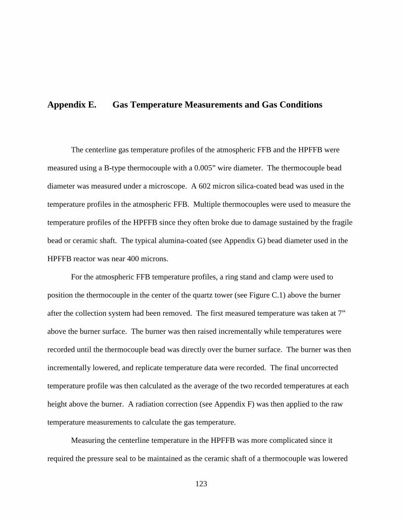
6.2 Pyrolysis and CO2 Gasification of Petroleum Coke
The pyrolysis and CO2 gasification of pet coke was studied from 1 to 15 atm using both
an atmospheric and pressurized flat-flame burner. All particle residence times during
experiments were less than 1.06 seconds. The pet coke CO2 gasification experiments at 10 and
15 atm were used to regress kinetic parameters for a 1st-order kinetic model. A comparison of
the measured CO2 gasification kinetics of pet coke with those in literature is also given.
6.2.1 Pyrolysis of Pet Coke
Figure 6.3 contains a summary of the data from all the pet coke pyrolysis experiments
according to mass release values calculated by a mass balance (see Table B.1 in the appendix).
A mass balance is obtained by weighing the collected char and comparing it to the weight of raw
pet coke fed. Every pet coke experiment run at 1, 2.5, and 5 atm yielded pyrolysis data since no
measurable amount of CO2 gasification occurred at these conditions in the range of particle
residence times of 23 to 753 ms. The pyrolysis data at 10 and 15 atm came from experiments at
low particle residence times (< 104 ms) as CO2 gasification occurred at higher residence times.
The ASTM volatiles value (shown by the dashed line in Figure 6.3) for pet coke appeared to be a
good approximation of the mass release experienced during pyrolysis in every case.
51
Other researchers found similar results when studying the pyrolysis of pet coke in a TGA
at lower heating rates. Zamalloa et al. (1995) observed that 10 wt% of the pet coke turned to
volatiles when heating it at 20 K/min under argon to a peak temperature of 1273 to 1473 K.
Although the proximate analysis of the pet coke used by Zamalloa et al. was not provided, the
ASTM voltatiles percent of 10 wt% is a good average value based on articles in the literature
where this information has been provided (Yoon et al., 2007; Zou et al., 2007; Fermoso et al.,
2009; Gu et al., 2009; Wu et al., 2009). Kocaefe et al. (1995) pyrolyzed 4 kinds of petroleum
coke with ASTM volatile yields ranging from 7.2 to 12 wt% in a TGA under N2 at a heating rate
of 146 K/min. It was observed that the ASTM volatiles yield was a good approximation of the
volatiles that escaped during pyrolysis in the TGA for each of the 4 varieties of pet coke. From
these TGA experiments as well as the experiments performed at BYU, the ASTM volatiles yield
of petroleum coke was a good estimate for the volatiles yield during both low and high heating-
rate experiments for experiments from 1-15 atm.
Figure 6.3. Pet coke pyrolysis data.
52
6.2.2 CO2 Gasification of Pet Coke Experiments
Experiments were conducted in the HPFFB to measure the gasification rate of pet coke
by CO2. A CO flame was used in all experiments with a small amount of hydrogen for flame
stability. This allowed CO2 gasification kinetics to be measured with only a minor presence of
H2O in the post-flame gas (< 1 mol%). This is important since H2O is also a gasifying agent.
Also, both CO and CO2 were present in the post-flame gas (see Table E.4), which represents
industrial conditions where CO inhibition of the CO2 gasification reaction occurs (Walker et al.,
1959; Revankar et al., 1987). CO strongly chemisorbs onto the pore surface of carbon and
retards the CO2 gasification rate (Turkdogan and Vinters, 1970).
CO2 gasification kinetics were intended to be calculated with mass release data obtained
by ash tracer analysis (see Section 4.6.1), which assumes that ash in the raw pet coke remains in
the char. It was originally thought that using data from an ash test was more accurate than a
mass balance (weighing char and how much pet coke was fed) because a mass balance can be
easily thrown off by spilling, clogging in the feed line, and by char collecting in other parts of the
reactor besides where it is intended. After a few months of pet coke experiments, it was noticed
that there was a large discrepancy between the mass release calculated by ash tracer and that
calculated by a mass balance at longer particle residence times. It was also noticed that the
repeatability of the mass release of pet coke at a given condition was better when calculated by a
mass balance than by ash tracer analysis. This is demonstrated in Figure 6.4, which was made
using replicate mass-release data of pet coke during pyrolysis collected in the atmospheric FFB
at a peak temperature of 1751 K. The average standard deviation between replicate runs at 1751
K was five times smaller (1.1% vs 5.4%) for the mass release values calculated by a mass
balance than it was when mass release was calculated by ash tracer analysis. This was largely
53
explained by ash leaving the char during the experiments. Vaporization of ash was a bigger
problem when char was collected at longer residence times. The CO2 gasification kinetics of pet
coke were consequently determined from data obtained by a mass balance rather than ash-tracer
analysis. Fortunately, this could be done because the weights of pet coke char had been recorded
as well as the amount of raw pet coke fed. Although it can sometimes be difficult to obtain an
accurate mass balance, it is believed that the mass release numbers calculated by a mass balance
are fairly accurate since (1) many replicate experiments were performed, (2) special care was
given to ensure the best mass balance possible, and (3) there was often good repeatability
between duplicate experiments. The best mass balance possible was ensured by shutting down
between different experimental conditions in order to clean out the collection system, and
weighing the amount of pet coke fed as well as the collected char.
Figure 6.4. Percent mass release of pet coke at 1751 K that was collected in the atmospheric FFB.
Figure 6.5 shows a summary of the data from all the pet coke experiments where CO2
gasification occurred based on mass release values determined by a mass balance (complete data
summarized in Table B.1). CO2 gasification of pet coke was only observed at 10 and 15 atm.
54
All pet coke experiments run at 1, 2.5, and 5 atm yielded pyrolysis data as no measurable amount
of CO2 gasification occurred at these conditions in the range of particle residence times of 23 to
753 ms. As can be seen in Figure 6.5, the mass release leveled off somewhere near a particle
residence time of 350 ms since the temperature decreased below 1500 K after 6” above the
burner in the majority of the HPFFB temperature profiles. Heaters were used in the HPFFB
when char is collected at the longer residence times (> 3” above the burner), but they could not
provide sufficiently hot temperatures for CO2 gasification of pet coke to continue.
Figure 6.5. Percent mass release during pet coke CO2 gasification experiments.
6.2.3 Modeling of Pet Coke CO2 Gasification
The CO2 gasification of pet coke was modeled using a simple first-order model, patterned
similarly after a previous oxidation model (Sowa, 2009). The rate expression was:
surfCOp
osurfCOrxnp
p PTREAPk
Adtdm
,2,2 exp1⋅
⋅−
⋅−=⋅−=⋅−
(6.1)
55
where Ap is the external surface area of the assumed-spherical particle, krxn is the rate constant of
CO2 gasification, PCO2, surf is the partial pressure of CO2 at the particle surface, Ao is the pre-
exponential factor, E is activation energy, R is the ideal gas constant, and Tp is the particle
temperature. The rate is negative since the particle lost mass during CO2 gasification. Equation
(6.1) was integrated using the Explicit Euler method for integration in an Excel spreadsheet. The
kinetic parameters A and E were determined by minimizing the error between predicted and
measured mass release of the pet coke particles. The measured mass release values of the pet
coke came from experiments in the HPFFB where the rate of change in the mass of the particles
were measured.
Although the model does not take pore diffusion into account, it does consider film
diffusion, which allowed PCO2,surf to be solved for explicitly.
( )surfCOCOmsurfCOrxn CChPk ,2,2,2 −⋅⋅=⋅− ∞ν (6.2) where ν is the mass of carbon (in grams) that react per mole of reactant, hm is the mass transfer
coefficient (Sh·DAB/dp), and CCO2,∞ is the concentration of CO2 in the bulk. In the case of CO2
gasification, ν was (12 g C/ mol CO2) from the following reaction:
C + CO2 2 CO
The mass transfer coefficient (hm) assumed a Sherwood number of 2, and used a Mitchell
correlation (Mitchell, 1980) for the diffusion coefficient (DAB) of CO2 in N2. The Sherwood
number can be assumed to equal 2 for small spheres traveling close to the gas velocity (Fletcher,
1989). Using the ideal-gas law for the concentration terms in Equation (6.2) (i.e., CCO2,∞ = PCO2,∞
/(R·Tgas) & CCO2,surf = PCO2,surf /(R·Tp) ) allowed PCO2,surf to be solved for:
56
⋅⋅
+⋅
⋅⋅= ∞
p
mrxngas
COmsurfCO
TRhkTR
PhP
ν
ν ,2,2
(6.3)
where PCO2,∞ was calculated as the product of the total pressure and the mole fraction of CO2 in
the post-flame gases predicted by thermodynamic equilibrium. Substituting Equation (6.3) into
Equation (6.1) allowed the rate per unit surface area to be solved as follows:
rxnp
gas
m
gas
surfCO
p
p
kTT
hTR
PAdt
dm
⋅+
⋅
⋅−
=⋅−
ν
,21 (6.4)
Since only the gas temperature (Tgas) was measured during experiments, Tp was solved for each
time step using an energy balance of the particle:
rxnp
psurrpppgaspcp
pp Hdt
dmTTATTAh
dtdT
Cm ∆⋅+−⋅⋅⋅+−⋅⋅=⋅⋅ )()( 44σε (6.5)
where mp is the mass of the particle, Cp is the heat capacity of the particle (Merrick, 1983), Tp is
the particle temperature, t is time, hc is the heat transfer coefficient (Nu·kgas/dp), Ap is the external
surface area of an assumed-spherical particle, εp is the emissivity of the char particle (εp =0.8
with the assumption that it was similar to that of coal char) (Fletcher, 1989), σ is the Stefan–
Boltzmann constant (5.67 x 10⁻¹² W/cm2/K), Tsurr is the temperature of the surroundings (500 K),
and ΔHrxn is the heat of reaction for the CO2 gasification reaction. The left-hand side of Equation
(6.5) was set equal to zero since steady state was assumed during the small time steps. The first
term on the right-hand side of Equation (6.5) represents the particle heating up from convective
heat transfer. The second term in Equation (6.5) is the radiative heat transfer from the particle,
which is negative since heat is leaving the particle. A more thorough analysis would have
included radiative heat transfer to the particle, as was done when correcting the centerline gas
57
temperature for radiation (see Appendix F). The last term in Equation (6.5) takes into account
the heat from the reacting particle, which is negative (from the dmp/dt term) due to the
endothermic CO2 gasification reaction. The Nusselt number (Nu) used in the heat transfer
coefficient in Equation (6.5) was assumed to equal 2 due to the low Reynolds number of the
small particle (~60 μm) traveling near the gas velocity. The thermal conductivity of the gas
(kgas) was assumed to equal that of N2 since it made up about 70 mol% of the post-flame gases.
The temperature dependence of the N2 thermal conductivity was taken into account using the
Mitchell correlation (Mitchell, 1980). The ΔHrxn term for the CO2 gasification reaction (C + CO2
2 CO) in Equation (6.5) was calculated at 25 °C as:
ΔH25°rxn = 2 ΔH°f,CO – ΔH°f,CO2 – ΔH°f,char
(6.6)
where H°f is the heat of formation at 25 °C. The Dulong formula (Green and Perry, 1984) was
used to calculate the heat of formation of the pet coke char (H°f,char). The Dulong formula is an
empirical equation that allows the calculation of the heat of combustion of a char from its
elemental composition for the reaction Cchar + O2 CO2. Since ΔHcombustion = - ΔHformation , the
heat of formation of char at 25 °C can be solved for as:
ΔH°f,char = ΔH°f,CO2 + ΔH°combustion,Dulong (6.7)
Substituting Equation (6.7) into Equation (6.6) allows the ΔHrxn term for the CO2 gasification
reaction in Equation (6.5) to be calculated at 25 °C as:
ΔH°rxn = 2 ΔH°f,CO – 2 ΔH°f,CO2 – ΔH°combustion,Dulong (6.8) The temperature dependence of the ΔHrxn term in Equation (6.5) was included by including the
∫ dTC p terms in Equation (6.6) for CO, CO2, and pet coke char using the Gordon McBride
database (McBride et al., 2002). The ∫ dTC p term for the pet coke char was simply assumed to
equal that of graphite using the temperature dependence of the Gordon McBride database. An
58
alternative would be to use H°f,graphite as a good approximation for the heat of formation of pet
coke char instead of using the Dulong formula to solve for it. The terms ΔH°f,graphite and ΔH°f,char
(by the Dulong formula) are about 6% different from each other, and using ΔH°f,graphite instead of
ΔH°f,char would have caused Tp values to increase anywhere from 6 to 30 K for the conditions
used in the HPFFB at 10 and 15 atm.
The particle temperature (Tp) was solved using Equation (6.5) using the Secant method
with 4 iterations. The time step (∆t) used in the spreadsheet was a function of a fixed change in
distance (dx) traveled by the particle:
pii v
dxttt =−=∆ −1 (6.9)
where vp is the particle velocity based on a measured particle velocity using a high speed camera
(see Appendix H). The particle mass (m) of each time step was calculated as:
⋅+=
⋅∆+= −
−−
− dtdm
vdxm
dtdm
tmm ip
pi
ipii
1,1
1,1
(6.10)
using Equation (6.4) for the (dmp/dt) term after multiplication by Ap. Gas temperature (Tgas) was
input into the spreadsheet as a function of height above the burner using an empirical polynomial
expression that fit the measured gas temperature. A changing particle diameter (dp) was included
using an empirical equation that was a function of height above the burner based on pet coke
diameter measurements (see Appendix K).
It is important when measuring kinetics at high temperature to make sure that the
measurements are not entirely controlled by film diffusion. The chi factor (Smith et al., 1994), χ,
was calculated for all the conditions since it provides an indication of the effect of film diffusion.
It is defined as the measured rate divided by the maximum rate under film-diffusion control
(when CCO2,surf is zero in Equation (6.2)):
59
( )
⋅⋅⋅
⋅=
⋅⋅
⋅=
∞∞
gas
COm
surfCOrxn
COm
surfCOrxn
TRP
h
PkCh
Pk
,2
,2
,2
,2
νν
χ
(6.11)
where PCO2,surf had the same definition as in Equation (6.3). The surface reaction controls when
χ is much less than 1. Film diffusion controls entirely when χ approaches 1. Mitchell et al.
(1992) set this cutoff at 0.9. In the 10 atm and 15 atm pet coke HPFFB experiments, χ ranged
from 0.2 to 0.35 and 0.55 to 0.7, respectively. These χ values mean that the measured kinetics
took place under Zone II conditions (Smith et al., 1994), which is a transition region between
surface-reaction control and film-diffusion control. The gasification pet coke kinetics measured
in the HPFFB were likely similar to those in a commercial entrained-flow gasifier since these
commercial reactors operate in Zone II conditions as well.
Five separate Excel worksheets were developed since there were 5 HPFFB conditions
where a measurable amount of CO2 gasification of pet coke occurred (10 atm: 1722K, 1967 K,
2139 K and 15 atm: 1681K, 1918 K). The pet coke experiments conducted at 1-5 atm were not
used to regress the kinetic parameters for the CO2 gasification reaction since no measurable
amount of gasification occurred at these conditions in the range of particle residence times of 23
to 753 ms. Pyrolysis data were used as initial points for modeling, and were taken from the
ASTM volatiles value when this information was not available. The experimental data that were
used to solve for the gasification kinetic parameters were largely the pet coke mass release
numbers calculated by mass balance. The mass release numbers calculated by ash tracer were
only used if they were close to the mass release numbers calculated by mass balance. This is
explained since ash sometimes vaporized from the pet coke char (see Section 6.2.2). Recall that
the mass release of the pet coke leveled off because the temperature of the reactor above a
certain point was not hot enough for continued CO2 gasification (see Figure 6.5). This was the
60
rationale for why experimental data of pet coke collected at 10” and 16.25” above the burner
were not used directly to determine the kinetic rate coefficients. The values of mass release from
the two aforementioned collection heights were still included to solve for the kinetic parameters,
but were averaged with the mass release data of the 6” collection height since the mass release of
pet coke at 6” above the burner was essentially the same as that of char collected at 10” or 16.25”
above the burner. The data used for modeling are summarized in Table 6.1.
Table 6.1. Pet coke CO2 gasification HPFFB data points used for modeling
The kinetic parameters were regressed using three data sets. The first data set included
only the 10 atm data (3 conditions). The second data set included only the 15 atm data (2
conditions), while the third data set used both the 10 atm and 15 atm data. In these three cases,
the pre-exponential factor varied while the activation energy was set to 140 kJ/mol based on CO2
gasification experiments on a TGA with a reaction order of 1 (Kwon et al., 1988). The regressed
rate parameters for the three data sets are summarized in Table 6.2. These parameters were
regressed from experiments with peak temperatures in the range of 1722-2139 K at partial
pressures of CO2 from 1.7 to 3.2 atm (see Appendix E). Figure 6.6 and Figure 6.7 show the
measured pet coke mass release data compared with that predicted by the gasification model
using kinetic parameters regressed from the first and second data sets, respectively.
61
Table 6.2. 1st-order kinetic rate coefficients for CO2 gasification of pet coke
E
(kJ/mol)
Ao
⋅⋅ 2
2 COatmscmCarbong
10 atm 140 118.4 15 atm 140 4289.3
10 & 15 atm 140 333.2
Figure 6.6. Comparison of 1st-order gasification model with measured pet coke data at 10 atm using Ao = 118.4 g∙cm-2∙s-1∙atm-1. The percent mass release is based on the wt% of daf pet coke.
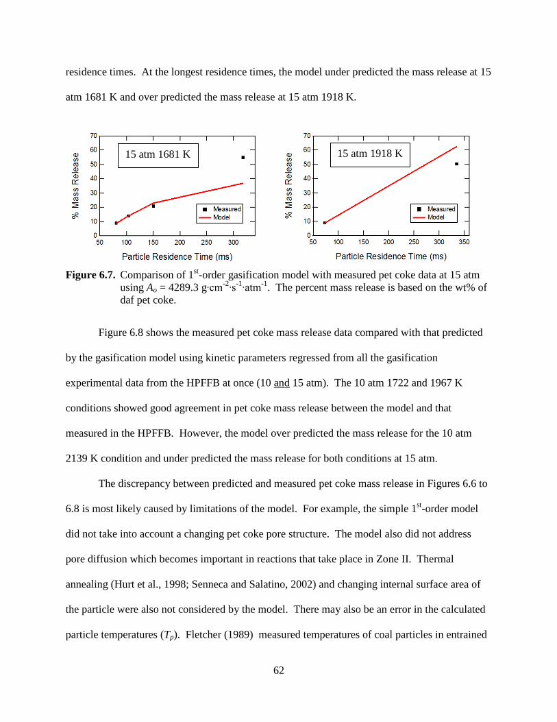
In Figure 6.6, the model under predicted the pet coke mass release at the 10 atm 1967 K
condition at long residence times. The model also over predicted the mass release at 10 atm
2139 K at the long residence time. In Figure 6.7, the model behaved similarly where there was
better agreement between the measured and predicted pet coke mass release values at low
10 atm 1722 K 10 atm 1967 K
10 atm 2139 K
62
residence times. At the longest residence times, the model under predicted the mass release at 15
atm 1681 K and over predicted the mass release at 15 atm 1918 K.
Figure 6.7. Comparison of 1st-order gasification model with measured pet coke data at 15 atm using Ao = 4289.3 g∙cm-2∙s-1∙atm-1. The percent mass release is based on the wt% of daf pet coke.
Figure 6.8 shows the measured pet coke mass release data compared with that predicted
by the gasification model using kinetic parameters regressed from all the gasification
experimental data from the HPFFB at once (10 and
The discrepancy between predicted and measured pet coke mass release in Figures 6.6 to
6.8 is most likely caused by limitations of the model. For example, the simple 1st-order model
did not take into account a changing pet coke pore structure. The model also did not address
pore diffusion which becomes important in reactions that take place in Zone II. Thermal
annealing (Hurt et al., 1998; Senneca and Salatino, 2002) and changing internal surface area of
the particle were also not considered by the model. There may also be an error in the calculated
particle temperatures (Tp). Fletcher (1989) measured temperatures of coal particles in entrained
15 atm). The 10 atm 1722 and 1967 K
conditions showed good agreement in pet coke mass release between the model and that
measured in the HPFFB. However, the model over predicted the mass release for the 10 atm
2139 K condition and under predicted the mass release for both conditions at 15 atm.
15 atm 1681 K 15 atm 1918 K
63
flow and observed that they were hotter than predicted by the energy balance in Equation (6.5)
near the injection point.
Figure 6.8. Comparison of 1st-order gasification model with measured pet coke data at 10 and 15 atm using Ao = 333.2 g∙cm-2∙s-1∙atm-1. The percent mass release is based on the wt% of daf pet coke.
An nth-order model (i.e., PCO2,surf
n in Eqn 6.1) would likely allow an improved fit of the
measured pet coke gasification data. Although an nth-order model requires iteration since
PCO2,surf in Equation (6.3) cannot be solved for explicitly, it would allow all the pet coke data at
10 atm 1722
10 atm 1967 K
10 atm 2139 K 15 atm 1681 K
15 atm 1918 K
64
1-15 atm to be explained. The fact that no extent of pet coke gasification was measured below
10 atm suggests that the rate has strong pressure dependence, implying that the order of n would
exceed unity in an nth-order model.
6.2.4 Comparison of Pet Coke CO2 Gasification Kinetics with Literature
Zamalloa et al. (1995) studied CO2 gasification kinetics from 1173 to 1573 K using a
TGA where the partial pressure of CO2 at the particle surface was 1 atm. The proposed rate that
is stated to cover the transition region from chemical control to pore diffusion control is:
⋅−
⋅=⋅TR
smgRate 143000exp8)/( 2
(6.12)
which uses a BET surface area and has units J/mol for the activation energy. The rate expression
in Equation (6.12) predicted that pet coke gasification by CO2 would not be observed in the short
residence times (<1 sec) of the HPFFB or FFB. This is consistent with the BYU pet coke data
that was measured at 1-5 atm (see Figure 6.3) since no measurable amount of gasification
occurred in these runs. Although pet coke was observed to gasify at 10 and 15 atm in the
HPFFB, this was not inconsistent with Zamalloa’s reported rate since the operating conditions of
the HPFFB at these cases were outside the range over which Zamalloa’s rate can be considered
valid (i.e., PCO2 in HPPFB > 1 atm).
The CO2 gasification reactivity of pet coke was also compared to that of coal. Goetz et
al. (1982) studied CO2 gasification kinetics of different ranks of coal up to 1720 K using a drop
tube furnace at atmospheric pressure with a CO2 partial pressure of 0.3 atm. Goetz et al. also
regressed kinetic parameters for a first-order CO2 gasification model on a basis of external
surface area, similarly as was done with the BYU pet coke data. The kinetic parameters of Goetz
et al. appear in Table 6.3.
65
Table 6.3. 1st-order kinetic rate coefficients for CO2 gasification of coal
Coal Name E
(kJ/mol)
Ao
⋅⋅ 2
2 COatmscmCarbong
Texas Lignite 165.34 660
Wyoming Wyodak 177.81 1040
The kinetics of Goetz et al. predicted that lignite and Wyodak coals would experience a
measurable amount (15 and 10 wt%, respectively) of CO2 gasification given 100 ms reaction
time at conditions similar to those run with pet coke in the BYU FFB reactor. This calculation
assumed PCO2,surf = 0.3 atm and a particle temperature of 1720 K. Since no CO2 gasification was
observed in the FFB pet coke experiments, it can be concluded that two ranks of coal are more
reactive than pet coke at these conditions. This is consistent with the literature where other
researchers have reported that the CO2 gasification reactivity of pet coke is lower than that of
coal based on experiments conducted at atmospheric pressure (Harris et al., 2006; Gu et al.,
2009; Wu et al., 2009).
When comparing the reactivities of two fuels, it is ideal if the same experiments are
performed on both fuels under identical conditions. Fortunately, Wyodak coal was run at some
of the same conditions in the HPFFB reactor as the pet coke (Shurtz, 2011). Gasification
experiments by CO2 were performed using Wyodak coal at 5, 10, and 15 atm in the HPFFB.
Unlike the pet coke which only pyrolyzed at 5 atm, the Wyodak coal experienced 64 wt%
gasification by 371 ms (based on mass of coal remaining after pyrolysis). However, comparing
the reactivities of pet coke and Wyodak coal solely based on the HPFFB experiments at 10 and
15 atm suggest that pet coke was more reactive. This conclusion assumed that no ash vaporized
from the coal, since the mass release of the Wyodak coal was calculated using an ash tracer (see
Section 4.6.1). The 1st-order CO2 gasification rate constants of pet coke and Wyodak coal are
66
plotted in Figure 6.9. The kinetic parameters in these rate constants were regressed as discussed
in Section 6.2.3 using 10 and 15 atm data from the HPFFB. In Figure 6.9, the Wyodak rate
constant used Ao and E values of 69.7 g/(cm2∙s∙atm) and 130 kJ/mol, respectively.
Figure 6.9. Comparison of 1st-order rate constant for CO2 gasification of pet coke and Wyodak coal based on 10 and 15 atm data in the HPFFB.
At partial pressures of CO2 less than 1 atm, the CO2 gasification reactivity of coal was higher
than that of pet coke. However, the reactivities of pet coke and Wyodak coal were on the same
order of magnitude from experiments with peak temperatures in the range of 1722-2139 K at
partial pressures of CO2 from 1.7 to 3.2 atm.
6.3 Pet Coke Ash Release
Ash was found to leave the pet coke, especially at longer residence times in the flat-flame
burner reactors (see Section 6.2.2). Figure 6.10 was made by calculating a percent error in ash
weight from a variety of conditions. This was done by calculating a percent error between the
67
measured amount of ash in a particular char sample and the predicted amount of ash that would
be present based on how much pet coke was fed. This method is only meaningful if a good mass
balance was obtained, which explains why only certain experimental conditions were included in
Figure 6.10. If pet coke char collected in other areas of the reactor besides the collection system,
this would shift all the points in Figure 6.10 up and lead to lower ash release numbers at the
longer residence times. A table of the data used to make this figure is included in Table B.2.
Figure 6.10. Percent error in ash weight of pet coke samples collected from a variety of conditions. Negative values imply vaporization of ash.
If the percent error in ash weight was +/- 2%, then it was recorded as 0% since 2% is the
accuracy of the scales at the low weights of ash measured (~8 mg of ash) after an ash test. The
accuracy of the scale at weights near 8 mg (typical ash weight) was determined by a scale
sensitivity experiment with the particular scale that was used to weigh ash samples. Figure 6.10
shows how much ash evaporated at a variety of conditions at all pressures from 1 to 15 atm in
the FFB and HPFFB. These data are included since they can be used to estimate the percentage
of ash that will leave the pet coke particle, thus allowing the design and/or operating conditions
68
of the gasifier to be adjusted accordingly. The evaporated ash may even be higher in an
industrial setting because the temperature drops off below 1500 K after 6” above the burner in
the majority of the temperature profiles of the HPFFB; this assumes that a hotter temperature
would lead to a greater amount of ash leaving the pet coke particle. Data points in Figure 6.10
with a negative percent error in ash weight (data below the solid black line) are representative of
chars that have experienced ash vaporization since this means that less ash was weighed than
was predicted from a particular char. It is very noticeable in the figure that ash evaporates at
longer residence times. The highest percentage of ash vaporization of the pet coke was observed
at the 15 atm 1681 K condition (~42 %). Figure 6.10 can be used directly to estimate the amount
of ash vaporization since -15% error in ash weight implies that 15% of the ash left the pet coke
particle.
The explanation of why several pet coke chars contained more ash at the lower residence
times than was predicted is left for further study, but may be explained by inhomogeneity of the
ash distributed in the pet coke. On one particular ash test of a pyrolyzed char collected at 76 ms
1683 K 2.5 atm, four times the expected ash was observed. The char was put back in the furnace
at 900 °C for another 5 hours, but the weight did not change. The appearance of this ash was
different from all the other pet coke ash tests. After a typical ash test of pet coke, black flakes
were found sticking to all sides of the crucible. The abnormal ash was light brown and collected
at the bottom of the crucible. Two other ash tests were performed on chars collected on different
days at 76 ms 1683 K 2.5 atm, but the very high ash content was not observed. This indicates
that the condition at which the char was collected did not factor in the high ash content, but was
more likely caused by ash inhomogeneity.
69
6.4 SEM Images of Pet Coke
Several SEM pictures of pet coke char are included in Figure 6.11. Recall that SEM
images of raw pet coke were included in Figure 4.2. In total, SEM images were taken of char
collected from 12 operating conditions at all pressures (1 to 15 atm) that included fully pyrolyzed
char as well as partially gasified char. There was no noticeable difference between fully
pyrolyzed char and partially gasified char; the char in Figure 6.11 that was collected at 15 atm
1918 K represents a partially gasified char. Only 4 SEM images are shown in Figure 6.11 since
all of the pet coke chars from the 12 different conditions closely resembled each other.
Figure 6.11. SEM images of pet coke char collected at various temperatures and pressures. The red circles are added to draw attention to the cracks in the pet coke.
70
The structure of the pet coke char appears to be very similar to that of raw pet coke, with
the only difference being that the char contains small cracks in its surface. This observation is
consistent with what other researchers have observed (Zamalloa and Utigard, 1995). The red
circles in Figure 6.11 are included to draw attention to some of these cracks on the char that was
collected at 2.5 atm; cracks are also present in the chars in Figure 6.11 that were collected at the
two 15 atm conditions although they are more difficult to see. Every pet coke char that was
observed under SEM contained these cracks; pressure was not believed to be an influencing
factor since the cracks were observed in pet coke chars that were collected at every pressure
condition (1 to 15 atm). Although the pet coke contains less than 10% volatiles, it is believed
that the cracks are likely a result of the volatiles escaping the particle interior quickly, which is
influenced by the high particle heating rates experienced in the flat-flame burner experiments.
Evidence of the high particle heating rates causing the cracks on the pet coke char is provided by
two observations. First, the char in Figure 6.11 that was collected at 15 atm 1431 K has less
cracks than several other chars. Since the peak temperature of this operating condition was
relatively cool, the particle heating rate was lower. This allowed more time for the volatiles to
escape the particle, which resulted in less cracks in the char’s surface. Second, pet coke char was
collected at 1320 K from the atmospheric FFB with twice the carrier N2 as usual in the feed tube.
The low temperature combined with the high carrier N2 were chosen to collect a char with a
lower heating rate. The SEM of this particular char is shown in Figure 6.11 and does not contain
any cracks. It is believed that the char collected at 1 atm 1320 K is fully pyrolyzed, although the
mass balance of this experiment was corrupted because some of the char spilled.
71
6.5 CO2 and N2 Surface Area of Pet Coke
Changing surface area is one factor that complicates heterogeneous char reactions. The
surface area affects gasification rates by influencing transport properties and the available
particle surface area that is able to react with the gasifying or oxidizing agent (Smith et al.,
1994). Chars with higher surface areas translate to higher gasification rates. Surface area data
also provide insight into what is happening to the particle structure during devolatilization and
gasification.
N2 and CO2 adsorption isotherms were used to measure the surface areas of pet coke
using a Micromeritics Tristar 3000 instrument. It is important to note that the N2 and CO2
surface area values are a measure of internal surface area, which is where most of the reactions
take place since the internal surface area greatly exceeds the external surface area. This is true as
long as the reaction is not film diffusion limited, which occurs at very high temperatures.
Nitrogen adsorption was conducted at 77 K (using liquid N2) in the N2 surface area
measurements that follow, and provides information regarding the mesopore (radii from 1-20
nm) structure. N2 surface areas that follow were calculated using the Brunauer-Emmett-Teller
(BET) equation. Carbon dioxide adsorption was performed at 298 K (using an ice water bath),
and provides insight regarding the micropores (radii < 1 nm) of the particle. CO2 surface areas
below were calculated using density functional theory (DFT), and represent the total area in the
pores greater than or equal to 4.54 angstroms.
The dashed and solid lines in Figures 6.12 to 6.14 represent the average surface area
value of raw pet coke and its corresponding 95% confidence interval of the population mean,
respectively.
72
The CO2 surface areas of pet coke char are shown in Figure 6.12 and Figure 6.13. Figure
6.12 shows CO2 surface area measurements of fully pyrolyzed pet coke chars that were collected
at 1, 2.5, and 5 atm. No CO2 gasification occurred at these conditions. The 1 atm pet coke chars
were collected from the atmospheric FFB, while the chars at the two higher pressure conditions
were collected from the HPFFB. It appears that temperature is the most influential factor on
surface area. The chars collected at the two lowest temperatures (2.5 atm 1683 K and 5 atm
1702 K) in Figure 6.12 had the highest surface area values, even slightly greater than that of raw
pet coke. It is interesting that the char from 2.5 atm 1876 K had a higher CO2 surface area than
the char collected at 1 atm 1751 K. The gas temperature profile in the 2.5 atm 1876 K condition
dropped off more quickly than the 1 atm 1751 K profile, which may explain the difference in
CO2 surface area. CO2 surface area of the pet coke chars in Figure 6.12 decrease with longer
residence time at the higher temperatures, leveling off to surface area values near 10% of that of
unreacted pet coke.
Figure 6.12. CO2 surface area of fully pyrolyzed pet coke chars collected at 1, 2.5, and 5 atm. The 1 atm chars were collected from the FFB, whereas all other chars were from the HPFFB.
73
The surface areas of chars collected at 10 and 15 atm from the HPFFB are shown in
Figure 6.13. The majority of these chars came from conditions where the char was partially
gasified except where indicated by open symbols which represent pyrolysis data. Mass release
data listed in Table B.1 (in the appendix) was used to distinguish between pyrolyzed char and
gasified char. It appears that temperature is the most influential factor of CO2 surface area from
this figure as well. The lowest surface area measurement came from char collected at the hottest
condition (10 atm 2139 K). CO2 surface area decreased with increased residence time at 10 atm
1967 K and 15 atm 1918 K, but not for the 15 atm 1681 K condition. A summary of all the CO2
surface area values of pet coke is located in Table B.3.
Figure 6.13. CO2 surface area of pet coke chars collected at 10 and 15 atm. Open symbols indicate pyrolyzed chars.
Figure 6.14 shows a plot of N2 surface area measurements taken from partially gasified
chars collected at 10 and 15 atm, except for a single pyrolysis char from 10 atm indicated by an
open symbol. At low residence times, the N2 surface area values increased to several times
higher than that of raw pet coke, but decreased with increasing residence time to values near or
74
slightly below the surface area of raw pet coke. This implies that the mesopore region of the pet
coke grows and then shrinks during CO2 gasification. Nothing can be said with certainty
concerning the mesopore region of the pet coke during pyrolysis since N2 surface area
measurements were not taken of the chars collected at 1 to 5 atm, but it is expected that a similar
trend would be observed. A summary of all the N2 surface area values of pet coke is located in
Table B.4.
The changing values of internal surface area in the pet coke chars can be explained by
growth and coalescence of pores. The internal surface area increases as the pores expand until
the pores become so large that they coalescence, thus leading to a decrease in internal surface
area (Dutta et al., 1977). The changing internal surface area of the pet coke chars is further
evidence that the experiments did not take place in a regime limited by film diffusion. When a
particle reaction is limited by film diffusion, the reaction takes place at the particle surface and
leaves the interior of the particle unchanged.
Figure 6.14. N2 surface area of partially gasified pet coke chars collected at 10 and 15 atm. The open symbol indicates a pyrolyzed char.
75
Tyler and Smith (1975) studied the CO2 gasification of pet coke from 1030 to 1180 K in
an atmospheric furnace using three different size fractions (2900, 900, 220 μm). They observed
that the N2 surface area of the pet coke had either remained unchanged or increased up to two
times the original surface area. The pet coke in their study was reacted up to 5 hours so the
effect of residence time was not known. The trend observed in Figure 6.14 is that longer
residence times (up to ~1 sec) caused the N2 surface area of the pet coke char to level off near
values of the unreacted pet coke. The discrepancy in trends can be explained by the differences
in reaction conditions. The experiments from the HPFFB were conducted at much lower particle
residence times (< 1 s), but operated at higher heating rates, temperature, and pressure. Zamalloa
and Utigard (1995) studied the CO2 gasification of pet coke from 1173 to 1573 K using a heating
rate of 20 K/min in an atmospheric TGA. The reaction time of these experiments was 30-40
minutes. The N2 surface area of the pet coke decreased with increasing temperature, which is the
same trend observed in by the experimental points near 350 ms of the 15 atm chars (1918 &
1681 K). Although no N2 surface area analysis was performed on any of the pyrolyzed pet coke
chars, Wu et al. (2009) found that a higher heating rate caused a decrease in the N2 surface area
of pyrolyzed pet coke. These experiments were conducted at 950 °C in an atmospheric furnace
using heating rates of 6 K/min and 650 K/s. A comparison of the pet coke CO2 surface areas
with the experiments of other researchers was not possible due to the lack of this data in the
literature.
A discussion of pet coke diameter ratios, apparent densities of pet coke chars, tar yields
during pet coke pyrolysis and gasification experiments, and elemental composition of pet coke
chars is given in Appendices K to N.
76
6.6 Summary
The pyrolysis and CO2 gasification of petroleum coke was studied from 1 to 15 atm using
both an atmospheric FFB and a HPFFB at peak temperatures from 1402 K to 2139 K. The
ASTM volatiles value of pet coke (8.78 % daf) appeared to be a good approximation of the mass
release experienced during pyrolysis in all experiments performed from 1 to 15 atm. Pet coke
CO2 gasification was only observed to occur at the 10 and 15 atm experiments, but not at lower
pressures. This suggests that the CO2 gasification rate of pet coke has strong pressure
dependence. Particle residence times in the reactor were less than 1.06 s in all experiments. The
apparent first-order Arrhenius pre-exponential factor and activation energy determined for CO2
gasification of pet coke were 333.2 g /cm2/s/atm and 140 kJ/mol, respectively. These parameters
were regressed from experiments with peak temperatures in the range of 1722-2139 K at partial
pressures of CO2 from 1.7 to 3.2 atm.
The measured pet coke CO2 gasification rates were compared with reported rates of pet
coke and coal in the literature, and found to be consistent. The gasification rate of pet coke was
also compared to Wyodak coal, since the two fuels were run separately in the HPFFB at the same
operating conditions. At operating pressures up to 5 atm and where PCO2 was less than 1.15 atm,
the CO2 gasification reactivity of Wyodak coal was higher than pet coke. However, the
reactivity of pet coke and Wyodak coal were on the same order of magnitude from experiments
at 10 and 15 atm where the peak temperature and PCO2 ranges were 1722-2139 K and 1.7-3.2
atm, respectively.
Ash was found to vaporize from the char during experiments, especially at longer
residence times. Up to 42 wt% of the ash in the pet coke was observed to leave the char, with
~20 wt% being an average value. SEM images of pet coke char revealed cracks in the char
77
surface at all pressures over a wide range of temperature conditions. These cracks are believed
to be caused as a result of the high particle heating rates of the flat-flame burners and are thought
to form as the volatiles quickly escape the interior of the pet coke particle. Besides these cracks,
both pyrolyzed and partially gasified pet coke char closely resembled the structure of raw pet
coke. Numerous surface area measurements (CO2 and N2) were taken of the pet coke chars
collected over a variety of conditions. Temperature appeared to have the most influence on the
surface area of the pet coke chars. A pet coke char collected from a hotter condition usually
resulted in a char with decreased surface area. Increased particle residence time also was
observed to lower the surface area of the pet coke chars. N2 surface area was only obtained on
partially gasified chars. At low residence times, the N2 surface area increased several fold when
compared to the N2 surface area of raw pet coke, but would then drop back down to values close
to the surface area of raw pet coke. This implies that the mesopore region of the pet coke grew
and then shrunk during CO2 gasification.
78
79
7. Error Analysis
The error analysis focuses on mass release since sawdust pyrolysis and CO2 gasification
of pet coke were the major research topics of this thesis. Recall that mass release was defined in
Section 4.6.
For the pyrolysis of sawdust, replicate ash tests were performed using sawdust chars that
had been collected from the FFB on different days in order to calculate replicate mass release
values (see Section 4.6.1). The results are shown in Table 7.1.
Table 7.1. Replicate ash-tracer mass release values during sawdust pyrolysis FFB experiments
Peak Temperature
(K)
Particle Residence Time
(ms)
% Mass Release (daf) by Ash Tracer
Standard Deviation
%
1163
55 97.8 96.8 96.6 96.7
0.6
1433
23 98.4 96.4
1.5
1433
31 98.9 98.7
0.1
The standard deviation (s) in Table 7.1 was calculated using N number of data points:
1
)(1
2
−
−=∑=
N
xxs
N
ii
(7.1)
where the arithmetic mean ( x ) of the individual data points (xi) was defined as:
80
∑=
=N
iix
Nx
1
1
(7.2)
There was very good repeatability in the sawdust mass release as indicated by the low standard
deviations (< 1.5 %) of ash-tracer mass release in Table 7.1.
The error analysis of the sawdust pyrolysis experiments was further investigated by
calculating the mass release using the inorganic tracers of Si, Al, and Ti (see Section 4.6.2) for a
single sawdust char collected from the FFB. This value was then compared to the mass-release
values obtained by ash tracer and a mass balance for the same condition (1163 K 55 ms), as
shown in Table 7.2. Mass release by inorganic tracers and ash tracer agreed within 1%, while
mass release by inorganic tracers and mass balance agree within 4%. This comparison was
performed for only one condition due to the costly task of collecting enough sawdust char to
perform an accurate ICP test.
Table 7.2. Mass release summary of the 1163 K 55 ms FFB sawdust case (daf basis)
% MR by Al, Si, Ti Tracers % MR by Ash Tracer % MR by Mass Balance Al 97.5%
97.3% 94.2% Si 99.1%
Ti 98.4%
The error analysis for the pet coke CO2 gasification experiments relied on mass release
values as determined by a mass balance (using weight of char collected and weight of raw pet
coke fed). Mass release values could not be calculated by ash tracer and inorganic tracers for pet
coke due to ash vaporization (see Section 6.3) and the absence of measurable quantities of Si, Al,
and Ti in the pet coke, respectively. Fortunately, mass release values for the pet coke
experiments could be calculated since the weights of pet coke char had been recorded as well as
the amount of raw pet coke fed. The best mass balance possible was ensured by shutting down
between different experimental conditions in order to clean out the collection system, and
81
weighing the amount of pet coke fed as well as the collected char. A summary of the mass
release pet coke CO2 gasification data is shown in Table 7.3 as calculated by a mass balance.
Table 7.3. Mass release summary of the pet coke CO2 gasification experiments in the HPFFB
Pressure (atm)
Peak Temperature
(K)
Particle Residence Time (ms)
% MR (daf) * by mass balance
Standard Deviation
%
10
1722
150 11.8 10.8
0.7
10
1967
663 34.8 36.6
1.3
10
1967
1061
26.2 48.1 43.3
11.5
15
1918
577 57.7 58.4
0.5
15
1918
994
38.0 44.5 52.6 50.0
6.5
The average standard deviation in pet coke mass release using all five experimental conditions
where replicate experiments had been performed was 4.1%. The 10 atm 1967 K condition at
1061 ms and the 15 atm 1918 K condition at 994 ms had the highest standard deviations in mass
release. Both of these conditions were run at the longest residence time possible for the
condition (with the collection probe positioned 16.25” above the burner). It is possible that some
pet coke char did not make it into the collection probe, but collected in other parts of the reactor
during some of these replicate runs. The replicate experiments in Table 7.3 showed very good
repeatability for mass release values determined by a mass balance. Mass release values
determined by ash tracer or inorganic tracers are thought to be more accurate, but were not
possible in this case.
82
83
8. Conclusions and Recommendations
8.1 Sawdust Pyrolysis Experiments
Sawdust pyrolysis experiments were performed on an atmospheric FFB at peak
temperatures of 1163, 1320, and 1433 K. The conclusions for these experiments are:
1) Sawdust mass release from devolatilization in the FFB exceeded the ASTM volatiles
value by 12%.
2) The low tar yields (< 3 wt%) are explained by secondary tar cracking that occurs above
500 °C. Although tar yields can be as high as 75 wt% following the primary pyrolysis of
wood, tar cracking caused the light gas to be the major product. The tar-cracking model
of Fagbemi et al. (2001) well predicted the sawdust tar yields measured on the FFB. The
pre-exponential factor and activation energy in Fagbemi’s model were 4.28x10⁶ s-1 and
107.5 kJ/mol, respectively.
3) From SEM images of the sawdust char, it was shown that the shape of the particles
continues to change even after mass release is complete.
4) The sawdust char particles were spherical with many voids and pores. The original
structure of the sawdust did not exist after devolatilization due to melting of the cell
structure and plastic transformations. The fact that sawdust particles turn spherical after
84
pyrolysis at high heating rates means that combustion or gasification of sawdust can be
modeled assuming spherical particles.
8.2 Biomass Pyrolysis Modeling
Sawdust pyrolysis was modeled using the CPD model combined with a tar-cracking
model. The conclusions for biomass modeling are:
1) This model satisfactorily predicted sawdust devolatilization yields for 5 different
sawdusts from 3 different reactors (flat-flame burner, fluidized bed, & drop-tube).
2) The biomass pyrolysis model is likely to fail when the parent biomass has high ash
content since it assumes that biomass devolatilization occurs as the weighted sum of its
3) The model performed better at predicting biomass pyrolysis yields from experiments with
a high heating rate. Otherwise, the predicted tar yields near 500 °C were too high.
8.3 Pet Coke Pyrolysis and CO2 Gasification Experiments
The pyrolysis and CO2 gasification of petroleum coke was studied from 1 to 15 atm using
both an atmospheric FFB and a HPFFB. The conclusions follow:
1) The ASTM volatiles value of pet coke appeared to be a good approximation of the mass
release experienced during pyrolysis in all experiments performed from 1 to 15 atm.
2) Ash was found to vaporize from the pet coke char during experiments, especially at
longer residence times. Up to 42 wt% of the ash in the pet coke was observed to leave
the char, with ~20 wt% being an average value.
85
3) SEM images of pet coke char revealed cracks in the char surface at all pressures over a
wide range of temperature conditions. These cracks are believed to be caused as a result
of the high particle heating rates of the flat-flame burners and are thought to form as the
volatiles quickly escape the interior of the pet coke particle. Besides these cracks, both
pyrolyzed and partially gasified pet coke char closely resembled the structure of raw pet
coke.
4) Temperature appeared to have the most influence on the surface area (CO2 and N2) of the
pet coke chars. A pet coke char collected from a hotter condition usually resulted in a
char with decreased surface area. Increased particle residence time also was observed to
lower the surface area of the pet coke chars. At low residence times, the N2 surface area
increased several fold when compared to the N2 surface area of raw pet coke, but would
then drop back down to values close to the surface area of raw pet coke. This implies
that the mesopore region of the pet coke grew and then shrunk during CO2 gasification.
8.4 Modeling of Pet Coke CO2 Gasification
A first-order model was used to regress Arrhenius kinetic parameters for the CO2
gasification of pet coke using measured mass release data from 10 and 15 atm HPFFB
experiments. The results of the modeling efforts follow:
1) The apparent first-order Arrhenius pre-exponential factor and activation energy for CO2
gasification of pet coke were 333.2 g Carbon/(cm2∙s∙atm CO2) and 140 kJ/mol,
respectively. These parameters were regressed from experiments with peak temperatures
in the range of 1722-2139 K at partial pressures from 1.7 to 3.2 atm.
86
2) The measured pet coke CO2 gasification rates were compared with reported rates of pet
coke and coal char in the literature, and found to be consistent. The gasification rate of
pet coke was also compared to Wyodak coal, since the two fuels were run separately in
the HPFFB at the same operating conditions. At operating pressures up to 5 atm and
where PCO2 was less than 1.15 atm, the CO2 gasification reactivity of Wyodak coal was
much higher than pet coke. However, the reactivity of pet coke and Wyodak coal were
on the same order of magnitude from experiments at 10 and 15 atm where the peak
temperature and PCO2 ranges were 1722-2139 K and 1.7-3.2 atm, respectively.
3) An nth-order model would likely allow an even better fit of the measured pet coke
gasification data. The fact that no extent of pet coke gasification by CO2 was measured
below 10 atm suggests that the rate has strong pressure dependence, implying that the
order of n would exceed unity in an nth-order model.
8.5 Recommendations
Listed below are several recommendations for future work based on knowledge gained
during this thesis project:
1) Develop a new method to measure the gas temperature profiles in the HPFFB. There
Improvements should be made to the safety of the HPFFB lab by changing the way
centerline gas temperature profiles are measured (see Appendix E). A rubber stopper was
used to maintain the pressure seal of the reactor up to 15 atm, but the danger of doing this
is leaking high concentrations of CO into the room if the seal fails. The ceramic shaft of
the thermocouple becomes a projectile if the seal between the rubber stopper and ceramic
87
shaft is compromised. It would be safer to develop a contraption where the thermocouple
shaft was held in place and hooked to a moveable track.
2) Install hotter heaters in the HPFFB reactor. The heaters in the HPFFB were only rated
to 1200 °C, which caused the temperature inside the reactor to level off near 1200-1300
°C during the experiments with long residence times (see Figure 6.2). These relatively
low temperatures may be adequate for combustion studies, but are not highly suitable for
gasification studies where the kinetics are orders of magnitude slower. The mass release
of the pet coke reached an asymptote at a collection height about 6 inches above the
burner (see Figure 6.5). Heaters rated to a higher temperature would allow a measurable
difference in gasification reactivity above 6” above the burner.
3) Increase the CO2 concentrations in the HPFFB reactor. A higher extent of CO2
gasification could have measured if a tank of CO2 was plumbed into the line where
oxidizer N2 was introduced in this project.
4) Be hesitant about future biomass studies using the atmospheric FFB. Sawdust
experiments in the FFB were very
5) Study biomass tar cracking at higher temperatures. It was noticed in the atmospheric
FFB experiments that there was a small fraction of the sawdust tar that did not thermally
crack into light gas (see Section
time consuming due to frequent clogging problems in
the narrow feeder tube, which could not be widened. The biomass experiments were
expensive in terms of man hours and costs of gases (mainly CO). Sawdust was fed at a
low feed rate of 0.50 g/hr, and a typical char yield per week was only 400 mg.
5.3). It would be interesting to see if sawdust tar cracks
at a higher temperature since the peak temperature of the experiments of this thesis was
only 1433 K. Cracking of tar is important since even low tar yields can cause problems
88
in industry by fouling and corroding equipment, causing damage to motors and turbines,
lowering catalyst efficiency, and condensing in transfer lines.
6) Study the char morphology changes during biomass pyrolysis for other types of biomass
besides sawdust. In this thesis, it was observed that the original structure of sawdust did
not exist after devolatilization due to the melting of the cell structure and plastic
transformations. It would be interesting to see if other types of biomass particles also
turn spherical after devolatilization at high initial heating rates.
7) Study the pet coke CO2 gasification reactivity at higher pressures in a TGA or drop tube
reactor. Nearly all the pet coke CO2 gasification studies in the literature have been
conducted at atmospheric pressure where the pet coke CO2 gasification reactivity is lower
than coal. In this thesis, it was noticed that the CO2 gasification reactivity of pet coke
had a strong pressure dependence that caused the pet coke to be as reactive as coal. It
would be interesting to find out if this same observation is true on other types of reactors
besides a flat-flame burner.
89
9. References
Antal, M. J., "Effects of Reactor Severity on the Gas-Phase Pyrolysis of Celulose-Derived and Kraft Lignin-Derived Volatile Matter," Industrial & Engineering Chemistry Product Research and Development, 22(2), 366-375 (1983).
Bahlawane, N., U. Struckmeier, T. S. Kasper and P. Osswald, "Noncatalytic Thermocouple
Coatings Produced with Chemical Vapor Deposition for Flame Temperature Measurements," Review of Scientific Instruments, 78(1) (2007).
Batchelder, H. R., R. M. Busche and W. P. Armstrong, "Kinetics of Coal Gasification,"
Industrial & Engineering Chemistry 45, 1856 (1953). Baumlin, S., F. Broust, M. Ferrer, N. Meunier, E. Marty and J. Lede, "The Continuous Self
Stirred Tank Reactor: Measurement of the Cracking Kinetics of Biomass Pyrolysis Vapours," Chemical Engineering Science, 60(1), 41-55 (2005).
Biagini, E., F. Barontini and L. Tognotti, "Devolatilization of Biomass Fuels and Biomass
Bird, B., W. Stewart and E. Lightfoot, Transport Phenomena, New York, John Wiley & Sons,
Inc. (2002). Brage, C., Q. H. Yu and K. Sjostrom, "Characteristics of Evolution of Tar from Wood Pyrolysis
in a Fixed-Bed Reactor," Fuel, 75(2), 213-219 (1996). Bridgwater, A. V., "The Technical and Economic-Feasibility of Biomass Gasification for Power-
Generation," Fuel, 74(5), 631-653 (1995). Bridgwater, A. V., "Renewable Fuels and Chemicals by Thermal Processing of Biomass,"
Chemical Engineering Journal, 91(2-3), 87-102 (2003). Bridgwater, A. V., "Biomass Fast Pyrolysis," Thermal Science, 8, 21-49 (2004). Caballero, J. A., R. Font and A. Marcilla, "Comparative Study of the Pyrolysis of Almond Shells
and Their Fractions, Holocellulose and Lignin. Product Yields and Kinetics," Thermochimica Acta, 276, 57-77 (1996).
90
Cetin, E., B. Moghtaderi, R. Gupta and T. F. Wall, "Influence of Pyrolysis Conditions on the
Structure and Gasification Reactivity of Biomass Chars," Fuel, 83(16), 2139-2150 (2004).
Couhert, C., J. M. Commandre and S. Salvador, "Is It Possible to Predict Gas Yields of Any
Biomass after Rapid Pyrolysis at High Temperature from Its Composition in Cellulose, Hemicellulose and Lignin?," Fuel, 88(3), 408-417 (2009).
Crawford, R. L., Lignin Biodegradation and Transformation, New York, John Wiley & Sons
(1981). Di Blasi, C., "Modeling Chemical and Physical Processes of Wood and Biomass Pyrolysis,"
Progress in Energy and Combustion Science, 34(1), 47-90 (2008). Dupont, C., J. M. Commandre, P. Gauthier, G. Boissonnet, S. Salvador and D. Schweich,
"Biomass Pyrolysis Experiments in an Analytical Entrained Flow Reactor between 1073 K and 1273 K," Fuel, 87(7), 1155-1164 (2008).
Dutta, S., C. Y. Wen and R. J. Belt, "Reactivity of Coal and Char .1. Carbon-Dioxide
Atmosphere," Industrial & Engineering Chemistry Process Design and Development, 16(1), 20-30 (1977).
Essenhigh, R. H., Fundamentals of Coal Combustion , in Chemistry of Coal Utilization, 2nd
suppl. vol. (M.A. Elliot, ed.), pp.1153-1312, Wiley, New York (1981). Fagbemi, L., L. Khezami and R. Capart, "Pyrolysis Products from Different Biomasses:
Application to the Thermal Cracking of Tar," Applied Energy, 69(4), 293-306 (2001). Fermoso, J., B. Arias, M. G. Plaza, C. Pevida, F. Rubiera, J. J. Pis, F. Garcia-Pena and P. Casero,
"High-Pressure Co-Gasification of Coal with Biomass and Petroleum Coke," Fuel Processing Technology, 90(7-8), 926-932 (2009).
Fletcher, T. H., "Time-Resolved Temperature-Measurements of Individual Coal Particles During
Devolatilization," Combustion Science and Technology, 63(1-3), 89-105 (1989). Fletcher, T. H., A. R. Kerstein, R. J. Pugmire, M. S. Solum and D. M. Grant, "Chemical
Percolation Model for Devolatilization .3. Direct Use of C-13 NMR Data to Predict Effects of Coal Type," Energy & Fuels, 6(4), 414-431 (1992).
Fletcher, T. H., J. L. Ma, J. R. Rigby, A. L. Brown and B. W. Webb, "Soot in Coal Combustion
Systems," Progress in Energy and Combustion Science, 23(3), 283-301 (1997). Gale, T. K., C. H. Bartholomew and T. H. Fletcher, "Decreases in the Swelling and Porosity of
Bituminous Coals During Devolatilization at High Heating Rates," Combustion and Flame, 100(1-2), 94-100 (1995).
91
Ginter, D. M., G. A. Somorjai and H. Heinemann, "Factors Affecting the Reactivity of Chars and
Cokes During Low-Temperature (640-Degrees-C) Steam Gasification," Energy & Fuels, 7(3), 393-398 (1993).
Goetz, G. J., N. Y. Nsakala, R. L. Patel and T. C. Lao, "Combustion and Gasification Kinetics of
Chars from Four Commercially Significant Coals of Varying Rank," Second Annual Contractors' Conference on Coal Gasification, Palo Alto, CA (1982).
Green, D. W. and R. H. Perry, Perry's Chemical Engineers' Handbook, 6th Edition (1984). Gu, J., S. Wu, Y. Wu and J. Gao, "CO2-Gasification Reactivity of Different Carbonaceous
Materials at Elevated Temperatures," Energy Sources Part A-Recovery Utilization and Environmental Effects, 31(3), 232-243 (2009).
Guerrero, A., M. P. Ruiz, M. U. Alzueta, R. Bilbao and A. Millera, "Pyrolysis of Eucalyptus at
Different Heating Rates: Studies of Char Characterization and Oxidative Reactivity," Journal of Analytical and Applied Pyrolysis, 74(1-2), 307-314 (2005).
Harris, D. J. and I. W. Smith, "Intrinsic Reactivity of Petroleum Coke and Brown Coal Char to
Carbon Dioxide, Steam and Oxygen," Twenty-Third International Symposium on Combustion, The Combustion Institute: 1185-1190 (1990).
Harris, D. J., D. G. Roberts and D. G. Henderson, "Gasification Behaviour of Australian Coals at
High Temperature and Pressure," Fuel, 85(2), 134-142 (2006). Higman, C. and M. v. d. Burgt, Gasification, London, Elsevier Science (2003). Hurt, R., J. K. Sun and M. Lunden, "A Kinetic Model of Carbon Burnout in Pulverized Coal
Combustion," Combustion and Flame, 113(1-2), 181-197 (1998). Hurt, R. H., D. R. Dudek, J. P. Longwell and A. F. Sarofim, "The Phenomenon of Gasification-
Induced Carbon Densification and Its Influence on Pore Structure Evolution," Carbon, 26(4), 433-449 (1988).
Incropera, F. P. and D. P. Dewitt, Fundamentals of Heat and Mass Transfer, Chicago, John
Jenkins, B. M., L. L. Baxter and T. R. Miles, "Combustion Properties of Biomass," Fuel
Processing Technology, 54(1-3), 17-46 (1998). Kang, B. S., K. H. Lee, H. J. Park, Y. K. Park and J. S. Kim, "Fast Pyrolysis of Radiata Pine in a
Bench Scale Plant with a Fluidized Bed: Influence of a Char Separation System and Reaction Conditions on the Production of Bio-Oil," Journal of Analytical and Applied Pyrolysis, 76(1-2), 32-37 (2006).
Karunanithi, P. N. a. T., "Kinetic Modeling in Biomas Pyrolysis - a Review," Journal of Applied
Sciences Research, 4(12), 1627-1636 (2008). Kaskan, W. E., "The Dependence of Flame Temperature on Mass Burning Velocity," Sixth
Symposium (International) on Combustion (1957). Katsuki, M., Y. Mizutani and Y. Matsumoto, "An Improved Thermocouple Technique for
Measurement of Fluctuating Temperatures in Flames," Combustion and Flame, 67(1), 27-36 (1987).
Kocaefe, D., A. Charette and L. Castonguay, "Green Coke Pyrolysis - Investigation of
Simultaneous Changes in Gas and Solid-Phases," Fuel, 74(6), 791-799 (1995). Koufopanos, C. A., G. Maschio and A. Lucchesi, "Kinetic Modeling of the Pyrolysis of Biomass
and Biomass Components," Canadian Journal of Chemical Engineering, 67(1), 75-84 (1989).
Koufopanos, C. A., N. Papayannakos, G. Maschio and A. Lucchesi, "Modeling of the Pyrolysis
of Biomass Particles - Studies of Kinetics, Thermal and Heat-Transfer Effects," Canadian Journal of Chemical Engineering, 69(4), 907-915 (1991).
Kwon, T. W., S. D. Kim and D. P. C. Fung, "Reaction-Kinetics of Char-CO2 Gasification," Fuel,
67(4), 530-535 (1988). Li, S. G., S. P. Xu, S. Q. Liu, C. Yang and Q. H. Lu, "Fast Pyrolysis of Biomass in Free-Fall
Reactor for Hydrogen-Rich Gas," Fuel Processing Technology, 85(8-10), 1201-1211 (2004).
93
Ma, J., "Soot Formation During Coal Pyrolysis," PhD Dissertation, Brigham Young University (1996).
McBride, B. J., M. Zehe and S. Gordon, "Nasa Glenn Coefficients for Calculating
Thermodynamic Properties of Individual Species," NASA TP-2002-215556 (2002). Merrick, D., "Mathematical-Models of the Thermal-Decomposition of Coal .2. Specific-Heats
and Heats of Reaction," Fuel, 62(5), 540-546 (1983). Milenkova, K. S., A. G. Borrego, D. Alvarez, J. Xiberta and R. Menendez, "Devolatilisation
Behaviour of Petroleum Coke under Pulverised Fuel Combustion Conditions," Fuel, 82(15-17), 1883-1891 (2003).
Miller, R. S. and J. Bellan, "A Generalized Biomass Pyrolysis Model Based on Superimposed
Cellulose, Hemicellulose and Lignin Kinetics," Combustion Science and Technology, 126(1-6), 97-137 (1997).
Mims, C. A., M. Neville, R. Quann and A. Sarofim, "Laboratory Study of Trace Element
Transformation During Coal Combustion," presented at the National 87th AIChE Meeting, August 19-22, Boston, MA (1979).
Mitchell, R. E., "A Theoretical Model of Chemically Reacting Recirculating Flow," Livermore,
CA. Sandia National Laboratory, SAND79-8236 (1980). Mitchell, R. E., R. H. Hurt, L. L. Baxter and D. R. Hardesty, "Compilation of Sandia Coal Char
Combustion Data and Kinetics Analyses: Milestone Report", Sandia Technical Report, SAND92-8208, Sandia National Laboratory, Livermore, CA (1992).
Mohan, D., C. U. Pittman and P. H. Steele, "Pyrolysis of Wood/Biomass for Bio-Oil: A Critical
Review," Energy & Fuels, 20(3), 848-889 (2006). Mok, W. S. L. and M. J. Antal, "Uncatalyzed Solvolysis of Whole Biomass Hemicellulose by
Monson, C. R., "Char Oxidation at Elevated Pressure," PhD Dissertation, Brigham Young
University (1992). Nunn, T. R., J. B. Howard, J. P. Longwell and W. A. Peters, "Product Compositions and Kinetics
in the Rapid Pyrolysis of Sweet Gum Hardwood," Industrial & Engineering Chemistry Process Design and Development, 24(3), 836-844 (1985).
Pond, H. R., T. H. Fletcher and L. L. Baxter, "Prediction of Tar and Light Gas During Pyrolysis
of Black Liquor and Biomass," 3rd Annual Joint Meeting of the U.S. Sections of the Combustion Institute, Chicago, IL (2003).
94
Ranzi, E., A. Cuoci, T. Faravelli, A. Frassoldati, G. Migliavacca, S. Pierucci and S. Sommariva, "Chemical Kinetics of Biomass Pyrolysis," Energy & Fuels, 22(6), 4292-4300 (2008).
Rath, J. and G. Staudinger, "Cracking Reactions of Tar from Pyrolysis of Spruce Wood," Fuel,
80(10), 1379-1389 (2001). Raveendran, K., A. Ganesh and K. C. Khilar, "Pyrolysis Characteristics of Biomass and Biomass
Components," Fuel, 75(8), 987-998 (1996). Revankar, V. V. S., A. N. Gokarn and L. K. Doraiswamy, "Studies in Catalytic Steam
Gasification of Petroleum Coke with Special Reference to the Effect of Particle-Size," Industrial & Engineering Chemistry Research, 26(5), 1018-1025 (1987).
Rowell, R. M., The Chemistry of Solid Wood, Washington D.C., American Chemical Society
(1984). Rowley, R. L., W. V. Wilding, J. L. Oscarson, Y. Yang and N. F. Giles, "Dippr Data
Compilation of Pure Chemical Properties, Design Institute for Physical Properties," Provo, Utah, Brigham Young University (2010).
Scott, D. S. and J. Piskorz, "The Flash Pyrolysis of Aspen-Poplar Wood," Canadian Journal of
Chemical Engineering, 60(5), 666-674 (1982). Scott, D. S. and J. Piskorz, "The Continuous Flash Pyrolysis of Biomass," Canadian Journal of
Chemical Engineering, 62(3), 404-412 (1984). Scott, D. S., J. Piskorz and D. Radlein, "Liquid Products from the Continuous Flash Pyrolysis of
Biomass," Industrial & Engineering Chemistry Process Design and Development, 24(3), 581-588 (1985).
Scott, D. S., J. Piskorz, M. A. Bergougnou, R. Graham and R. P. Overend, "The Role of
Temperature In the Fast Pyrolysis of Cellulose and Wood," Industrial & Engineering Chemistry Research, 27(1), 8-15 (1988).
Senneca, O. and P. Salatino, "Loss of Gasification Reactivity toward O2 and CO2 Upon Heat
Treatment of Carbons," Proceedings of the Combustion Institute, 29, 485-493 (2002). Shaddix, C. R., "Correcting Thermocouple Measurements for Radiation Loss: A Critical
Review," Proceedings of the 33rd National Heat Transfer Conference, Albuquerque, New Mexico (1999).
Sheng, C. D. and J. L. T. Azevedo, "Modeling Biomass Devolatilization Using the Chemical
Percolation Devolatilization Model for the Main Components," Proceedings of the Combustion Institute, 29, 407-414 (2002).
95
Shurtz, R., "Pressurized Coal Pyrolysis and Gasification at High Initial Heating Rates," presented at the ACERC Conference, Feb. 25, Provo, UT (2010).
Shurtz, R., "Effects of Pressure on the Properties of Coal Char and Soot under Gasification
Conditions at High Initial Heating Rates," PhD Dissertation, Brigham Young University (In Progress 2011).
Siegel, R. and J. Howell, Thermal Radiation Heat Transfer, New York, Hemisphere Publishing
Corporation (1981). Smith, K. L., L. D. Smoot, T. H. Fletcher and R. J. Pugmire, The Structure and Reaction
Processes of Coal, New York, Plenum Press (1994). Smoot, L. D. and P. J. Smith, Coal Combustion and Gasification, New York, Plenum Press
(1985). Smoot, L. D., Fundamentals of Coal Combustion for Clean and Efficient Use, (Coal Science and
Technology 20), Amsterdam, Elsevier (1993). Solomon, P. R., D. G. Hamblen, R. M. Carangelo and J. L. Krause, "Coal Thermal
Decomposition in an Entrained Flow Reactor: Experiments and Theory," Nineteenth International Symposium on Combustion, The Combustion Institute, Pittsburgh, PA (1982).
Soltes, E. J. and T. J. Elder, Pyrolysis. In Organic Chemicals from Biomass, Boca Raton, FL,
CRC Press (1981). Sowa, J. M., "Studies of Coal Nitrogen Release Chemistry for Oxyfuel Combustion and
Chemical Additives," M.S. Thesis, Chemical Engineering, Brigham Young University (2009).
Sricharoenchaikul, V., PhD Dissertation, Georgia Institute of Technology (2001). Stiles, H. N. and R. Kandiyoti, "Secondary Reactions of Flash Pyrolysis Tars Measured in a
Fluidized-Bed Pyrolysis Reactor with Some Novel Design-Features," Fuel, 68(3), 275-282 (1989).
Sun, L. and B. X. Shen, "Microcrystallite Structural Changes of Petroleum Coke During the
Course of Carbonization Analyzed by X-Ray Diffraction," Petroleum Processing Section, 20, 53-56 (2004).
Trommer, D. and A. Steinfeld, "Kinetic Modeling for the Combined Pyrolysis and Steam
Gasification of Petroleum Coke and Experimental Determination of the Rate Constants by Dynamic Thermogravimetry in the 500-1520 K Range," Energy & Fuels, 20(3), 1250-1258 (2006).
96
Tsai, C. Y. and A. W. Scaroni, "The Structural-Changes of Bituminous Coal Particles During the Initial-Stages of Pulverized-Coal Combustion," Fuel, 66(2), 200-206 (1987).
Turkdogan, E. T. and J. V. Vinters, "Effect of Carbon Monoxide on the Rate of Oxidation of
Charcoal, Graphite and Coke in Carbon Dioxide," Carbon, 8, 39-53 (1970). Tyler, R. J. and I. W. Smith, "Reactivity of Petroleum Coke to Carbon Dioxide between 1030
and 1180 K," Fuel, 54(2), 99-104 (1975). Vassilatos, V., G. Taralas, K. Sjostrom and E. Bjornbom, "Catalytic Cracking of Tar in Biomass
Pyrolysis-Gas in the Presence of Calcined Dolomite," Canadian Journal of Chemical Engineering, 70(5), 1008-1013 (1992).
Vizzini, G., E. B. A. Bardi, M. Calcitelli and L. Tognotti, "Prediction of Rapid Biomass
Devolatilization Yields with an Upgraded Version of the Bio-CPD Model," 31st Meeting of the Italian Section of the Combustion Institute, Torino, Italy (2008).
Wagenaar, M., W. Prins and W. P. M. Vanswaaij, "Flash Pyrolysis Kinetics of Pine Wood," Fuel
Processing Technology, 36(1-3), 291-298 (1993). Walker, P. L., F. J. Rusinko and L. G. Austin, "Gas Reactions of Carbon," Advances in
Catalysis, 11, 133-221 (1959). Williams, T. C. and C. R. Shaddix, "Contamination of Carbon Monoxide with Metal Carbonyls:
Implications for Combustion Research," Combustion Science and Technology, 179(6), 1225-1230 (2007).
Wu, Y. Q., S. Y. Wu, J. Gu and J. S. Gao, "Differences in Physical Properties and CO2
Gasification Reactivity between Coal Char and Petroleum Coke," Process Safety and Environmental Protection, 87(5), 323-330 (2009).
Wurzenberger, J. C., S. Wallner, H. Raupenstrauch and J. G. Khinast, "Thermal Conversion of
where Fij is the appropriate view factor, which is also referred to as a configuration or shape
factor. The view factor is defined as the fraction of the radiation leaving surface i that is
intercepted by surface j (Incropera and Dewitt, 2002). F13 is the fraction of the radiation that
leaves the thermocouple bead and is intercepted by the collection probe if 1 and 3 are represented
by the thermocouple bead and collection probe, respectively. Tsurroundings in Equation (F.10) is the
temperature of the surroundings, which was assumed to be 500 K except when accounting for
radiation of the thermocouple bead to the heater walls. In this case, the Tsurroundings was taken as
the measured temperature of the heater wall provided by six K-type thermocouples placed at
various heights above the burner positioned between the quartz tube and the heaters (refer to
Figure F.2). There were four view factors used, referred to as F12, F13, F14, and F15. Figure F.2 is
provided as a visual aid for the following definitions. F12 refers to bead-to-burner view factor
(between pink dotted lines in Figure F.2); F13 refers to the bead-to-probe view factor (between
turquise dotted lines); F14 refers to the view factor from bead to vessel walls and insulation in the
lower HPFFB chamber (between pink & black dotted lines depicted by red arrows); and F15
refers to the view factor of the bead to everywhere else, but mostly is the bead-to-heater wall
view factor (between turquoise & black dotted lines depicted by blue arrows).
Sphere-to-disk view factors (Siegel and Howell, 1981) were used to solve for F12, F13,
and F14 while F15 was determined by difference since view factors sum to unity in an enclosure.
Figure F.1 and Equation (F.11) are provided as further explanation of the sphere-to-disk view
factors in the generic situation where rA is the sphere radius (thermocouple bead) and rB is the
disk radius (burner, collection probe, or heaters in the case of the HPPFB geometry).
136
Figure F.1. Sphere-to-disk view factor schematic that relates to Equation (F.11).
+
−=2
1
1121
hr
FB
AB
(F.11)
The calculation of F14 requires further explanation since this view factor is calculated
differently when the thermocouple bead is lower than ½” from the burner surface since the
thermocouple bead is below the heaters. For ease in explaining, F16 is defined as the view factor
of the thermocouple bead to the bottom portion of the HPFFB through the imaginary disc created
by the bottom portion of the heaters (between black dotted lines in Figure F.2), and F17 is the
view factor of the bead to the upper portion of the HPFFB through the imaginary disc created by
the bottom portion of the heaters when the thermocouple bead is less than ½” from the burner. If
the bead is positioned above the heaters (≥ ½” above the burner), F14 is calculated by the
difference between F16 and F12. If the thermocouple bead is below the heaters (≤ ½” above the
burner), F14 is calculated as the summation of F17 and F12 subtracted from unity since view
factors sum to one in an enclosure. Figure F.3 is included since it helps to easily visualize which
view factors are important at different heights above the burner. For example, F13 (bead-to-probe
view factor) becomes important when the thermocouple bead is about 2.5” away from the
collection probe, but otherwise is essentially zero. F12 (bead-to-burner view factor) is important
only when the thermocouple bead is less than 2” away from the burner, and so on.
h
rA
rB
137
Figure F.2. HPFFB during temperature measurements with an assumed-spherical
thermocouple bead. Dotted lines aid in the explanation of the sphere-to-disc view factors used in correcting the measured temperature for radiation losses from the thermocouple bead (see above text).
Figure F.3. View factors in the HPFFB when the probe is situated 16.25” above the burner.
138
139
Appendix G. Coating Thermocouple Beads by Vapor Deposition
Platinum-based thermocouples are very common in combustion/gasification experiments
due to their stability in high temperatures, and their resistance to attack in both reducing and
oxidizing environments (Shaddix, 1999). The problem that arises is that platinum is catalytic and
the energy balance used to correct thermocouple measurements for radiation loss in Appendix F
becomes more difficult due to the effects of catalytic heating. Catalytic heating is more prevalent
near the flame since catalytic activity is expected in the chemically nonequilibrium part of a
reactive flow (Katsuki et al., 1987). Silica, alumina, and BeO/Y2O3 are the typical non-catalytic
coatings used on thermocouple beads to alleviate the aforementioned problem.
Temperatures were measured in the HPFFB using an alumina-coated thermocouple bead.
The method of coating the bead involved an apparatus that allowed alumina to be deposited on
the bead through chemical vapor deposition based on a recent article by Bahlawane et al. (2007).
The basic idea was to get AlCl3 to react with oxygen in the air to form an alumina coating on the
thermocouple bead. The experimental setup and the inner workings of BYU’s thermocouple
bead coating apparatus are shown in Figure G.1 and Figure G.2, respectively. To coat a
thermocouple bead, a heated cord was wrapped around the metal housing that contained the
AlCl3 in order to raise the AlCl3 vapor pressure by increasing its temperature. A K-type
thermocouple was placed between the heated cord and surrounding insulation in order to
measure the AlCl3 temperature. A variable power supply allowed control of the heated cord, and
140
was adjusted until the K-type thermocouple read values near 135 °C. A vacuum pulled a
controlled amount of air from the inlet through a needle valve, while another variable power
supply allowed control of the deposition temperature of alumina on the thermocouple bead. The
electrical current through the thermocouple bead was adjusted until the bead glowed brightly
through the viewport. A deposition time up to 2 hours can be required to ensure a good coating
on the thermocouple bead.
Although the apparatus was made out of PVC, it could have easily been made out of
metal. This change would have allowed a higher vacuum to be drawn on the system, thus
increasing both the partial pressure of AlCl3 and alumina deposition on the thermocouple bead.
Figure G.1. Apparatus used to coat thermocouple beads with an alumina coating by chemical vapor deposition. ‘A’ is the variable power supply used to pass current though the thermocouple bead; ‘B’ is a K-type thermocouple reader that measured the temperature of the AlCl3; ‘C’ is the power supply to the heating cord wrapped around the metal housing that contained the AlCl3; ‘D’ is the outlet line hooked to a vacuum; ‘E’ is the viewport that allowed optical access to the glowing thermocouple bead; ‘F’ is a pressure gauge; ‘G’ is where the AlCl3 was encased in a metal housing surrounded by heating cord & insulation; and ‘H’ is the needle valve which controlled the amount of air pulled into the system.
141
The apparatus also allowed a thermocouple bead to be coated after it had become part of a
finished thermocouple through the top T-fitting. In this scenario, a rubber stopper with a center
hole was placed around the ceramic shaft of the thermocouple and was held down by a nut in
order to maintain a vacuum on the system.
Figure G.2. Inside workings of the thermocouple bead coater. The red line represents where thermocouple bead would be positioned during the coating process.
A simple electrolysis test was performed to ensure the coating of a thermocouple bead, as
displayed in Figure G.3. The bead of a finished thermocouple was placed in a water and NaOH
solution in a beaker. An electrical circuit was created using wire, two 1.5-volt batteries, and the
thermocouple. A proper coating of the thermocouple bead was ensured if no bubbles formed on
the bead. Note that the schematic in Figure G.3 is not drawn to scale.
142
Figure G.3. Experimental setup to test if a thermocouple bead was successfully coated.
143
Appendix H. Measured Particle Velocities in FFB and HPFFB Reactors
Measuring particle velocities allowed the calculation of particle residence time, which
was used to determine gasification kinetics and also to evaluate pyrolysis models. A high-speed
camera (Kodak EktaPro) was used to measure sawdust and pet coke velocities in the FFB and the
HPFFB. The camera allowed particles to be filmed up to 1000 frames per second (fps), but
particles were typically only filmed up to 250 fps since the lower frame speeds allowed dimmer
particles to be measured while also enabling longer record times. After filming, the recorded
particle movement was played on a monitor and the distance a particle traveled in one frame was
measured on the screen. The relationship between apparent distance traveled and actual distance
traveled was obtained by measuring an object of known length on the monitor, and calculating
accordingly. The particle velocity was then obtained by dividing the distance traveled by the
time of a single frame (1/50, 1/125, or 1/250 sec). Particle velocities at a single height above the
burner were taken as the average of at least 5 different particles.
Theoretical calculations were necessary to obtain particle residence times since the
particles could not be filmed over the entire particle path. In the HPFFB, a 9/16” viewport offers
the sole optical access into the reactor. In the FFB, the first measured particle velocities were
obtained about 1” above the burner surface. Thus theoretical calculations were necessary to
bridge the gap where particle velocities could not be measured.
144
The equations used to predict particle velocities begin with a simple force balance on the
particle taking into account the forces due to gravity, buoyancy, and drag (see
Theoretical Particle Velocity Model
A simple model was used to predict particle velocities when particles could not be
filmed. The model was based on the assumption that all particles were spherical, whether they
were pet coke or sawdust. Particle interactions were ignored, justified by the slow feed rate (0.5
to 1.3 g/hr) that ensured single particle behavior. Lastly, the model assumed that there was no
change in particle mass or diameter. A quadratic scaling factor was used in order to transition
from a purely theoretical particle velocity at the burner inlet to a measured particle velocity,
typically about 1 inch above the burner surface.
Figure H.1).
Figure H.1. Depiction of the forces on a single particle as the particles travel from the burner to
the collection probe.
Equation (H.1) gives the definition of force, while Equation (H.2) is simply the
rearrangement of Equation (H.1) in order to solve for acceleration (a), where vp is the particle
velocity, t is time, Fdrag is the drag force, Fbuoyancy is the buoyancy force, Fgravity is the force on the
particle due to gravity, mp is the particle mass, dp is the particle diameter, and ρp is the particle
Fgravity
Fbuoyancy Fdrag
145
density. The diameters of sawdust and pet coke used in the model were 75 and 60 microns,
respectively. Densities of sawdust and pet coke were taken as 650 kg/m3 (Koufopanos et al.,
1991) and 1750 kg/m3 (measured), respectively.
onacceleratimassForce ×=∑
(H.1)
( ) ( )
pp
gravitybuoyancydrag
p
gravitybuoyancydragp
d
FFFm
FFFdt
dva
ρπ
⋅
⋅
−+=
−+==
6
3
(H.2)
The general drag force correlation used was (Bird et al., 2002):
( ) ( )dgasdrag CareasurfacewettedvF ⋅⋅
⋅⋅= ∞
2
21 ρ
(H.3)
where ρgas is the gas density, Cd is the drag coefficient, and the wetted surface area is taken as
the area obtained when projecting the solid onto a plane perpendicular to the fluid flow (π∙dp2/4).
The term v∞ is the slip velocity between the entrainment gas and the particle and is defined as:
pgas vvv −=∞
(H.4)
where vgas is the gas velocity and vp is the particle velocity. The gas velocity was predicted as:
burnergas
gasgas A
mv
⋅=ρ
(H.5)
where gasm is the gas mass flow rate, and Aburner is the cross-sectional area of the flow path
through which the post-combustion gases travel before entering the collection probe. The gas
density, ρgas, is defined using the ideal-gas law as:
gasgas MWTR
P⋅
⋅=ρ
(H.6)
146
where P is pressure, R is the ideal-gas constant, T is temperature, and MWgas is the average gas
molecular weight of the post-combustion products predicted by thermodynamic equilibrium.
The correlation used for Cd in Equation (H.3) is:
2
5407.0Re24
+=dC
(H.7)
which is for a sphere up to a Reynolds number (Re = ρgas·dp·v∞/ μgas) of 6000 (Bird et al., 2002).
The dynamic gas viscosity (μgas) was calculated using the following empirical correlation:
[ ] sec1095.1)(1025.2 58 ⋅×+×= −− PaTgasµ
(H.8) where the temperature is in Kelvin. The correlation in Equation (H.8) was developed after
plotting the gas viscosity from several conditions from both the HPFFB and the FFB and
noticing a linear trend (see Figure H.2). The gas viscosity at a given condition in Figure H.2 was
calculated using DIPPR correlations (Rowley et al., 2010) to predict the viscosity of individual
post-combustion gas products (N2, CO2, CO, H2O, H2, Ar) and then calculating the molar
weighted average as determined by the predicted products from thermodynamic equilibrium.
Figure H.2. Visual comparison of how well Equation (H.8) predicts gas viscosity at experimental conditions from the FFB and the HPFFB.
147
The equations for the forces of buoyancy and gravity are:
gd
F gasp
buoyancy ⋅⋅
⋅= ρ
π6
3
(H.9)
gd
F pp
gravity ⋅⋅
⋅= ρ
π6
3
(H.10)
where g is taken as 9.81 m/s2 and all other terms carry the aforementioned definitions.
Substituting Equations (H.3), (H.4), (H.7), (H.9), and (H.10) into (H.2) yields Equation (H.11)
after simple rearrangement.
( )
−⋅+
+
⋅
−⋅== 15407.0
Re24
43
22
p
gas
ppgas
p
gasp gd
vvdt
dva
ρρ
ρρ
(H.11)
Equation (H.11) would be simpler if Stoke’s flow was assumed, but this assumption was not
made since the Reynolds number of the particle was greater than 0.1 (Bird et al., 2002).
Equation (H.12) is the definition of particle velocity where z is the distance above the burner.
pvdtdz
=
(H.12)
Equations (H.11) and (H.12) were plugged into Polymath, a program capable of solving
differential equations. A Runge-Kutta-Fehlberg ODE solver was used to solve for the theoretical
particle velocity profiles. Calculating particle velocity required an initial velocity at the burner
surface, which was taken as the terminal velocity in the feed tube which runs from the feeder to
the burner. This velocity was solved for by equating Equation (H.11) to zero and solving for vp
using N2 gas properties (carrier gas in feed tube) and using the cross-sectional area of the feed
tube when solving for vgas. The FFB and HPFFB feed tube inside diameters were 0.053” and
0.041”, respectively.
148
Separate Polymath files were created for each experimental condition by entering the
appropriate operating pressure, measured temperature profile, gas mass flow rate, and post-
combustion gas molecular weight. Each individual temperature profile from the FFB and the
HPFFB was entered into its respective Polymath file as a function of z after fitting the measured
temperature profile in Excel to a polynomial equation.
The entire particle velocity profile in the HPFFB could not be measured since a small
viewport (9/16” diameter) about 1” above the burner surface provided the sole optical access into
the HPFFB. A high-speed camera was used to measure particle velocities through this viewport
at a maximum of two different heights above the burner surface. These particle velocity
measurements in the HPFFB were taken at a maximum height about ¾” above the burner surface
and are included near the end of
HPFFB Particle Velocity Measurements
Appendix H.
A method was developed to predict the entire HPFFB particle velocity profile with a
single velocity measurement. The scheme used a quadratic scaling factor to transition from a
theoretical particle velocity to a measured particle velocity, and then scaled by the centerline gas
temperature to predict the particle velocity beyond the height at which the maximum particle
velocity had been measured.
The quadratic scaling factor, f, was a function of the height above the burner and was
multiplied by the theoretical particle velocity to estimate the true particle velocity up to the
maximum height above the burner at which a particle velocity measurement had been taken
(usually ~¾”):
ltheoreticapvhfv ,)( ⋅=
(H.13)
149
where vp,theoretical is the predicted particle velocity from using Equations (H.11) and (H.12). The
equation for f took the form:
112
1)( chbhahf +⋅+⋅=
(H.14) where h is the height above the burner up to the maximum height at which a particle velocity had
been measured in the HPFFB. The constants a1, b1, and c1 could be solved using two boundary
conditions, assuming that the maximum particle velocity occurred about ¾” off the burner
surface. This was the height at which particle velocity was measured and was also near the
maximum measured centerline temperature. The boundary conditions and definition of
maximum f follow:
1)0( =f (H.15)
ltheoreticap
measuredpratio v
vmLf
,
,)( ==
(H.16)
1120 bLadhdf
L +⋅==
(H.17)
where L is the maximum height above the burner at which a particle velocity was measured, and
mratio is the ratio of the measured particle velocity to the theoretical particle velocity (see Eqns
(H.11) & (H.12)) at height L. The average value of mratio over the many different HPFFB
conditions was 2.06, but ranged from 1.03 to 3.45. The first boundary condition suggests that
the theoretical particle velocity was used at the burner surface, which was taken as the
theoretical, terminal particle velocity in the feed tube. The second boundary condition defines
mratio, and Equation (H.17) resulted from assuming that the maximum particle velocity took place
at height L. The constants a, b, and c could be solved using the two boundary conditions and
definition of maximum as:
Lma ratio−
=1
1
(H.18)
150
( )L
mb ratio 121
−⋅=
(H.19)
11 =c
(H.20)
where all terms retain their aforementioned definitions. Equations (H.18) through (H.20)
provided a closed-form solution to the quadratic scaling factor (see Eqn (H.14)).
The particle velocity beyond the height where the particle velocity had been measured in
the HPFFB was scaled by temperature. This originated from a simple derivation based on the
ratios of gas mass flow rate from 2 conditions, assuming that vgas was a good approximation of
where Aflowpath is the cross-sectional area of the flow path and all other terms carry their
aforementioned definitions. Using the definition of density from the ideal gas law and assuming
that the cross-sectional area terms from the 2 conditions were equal, Equation (H.23) results.
2
1
1
2
1
212 MW
MWmm
TTvv
gas
gaspp ⋅⋅⋅≈
(H.23)
The following equation was used to predict the velocity profile beyond the maximum height
above the HPFFB burner at which a particle velocity had been measured and is the result of
Equation (H.23) when the 2 reference points came from the same operating condition:
refrefpp T
hTvhv )()( 1,1 ⋅=
(H.24)
151
where h1 is the height above the burner from L to the collection probe height, and T is the
measured centerline gas temperature. The reference point (vp & T) for each condition was the
measured particle velocity at the maximum measured height above the burner (< 1”) and the
associated centerline gas temperature at this height. Equation (H.24) scaled the remaining
particle velocity profile by gas temperature.
A lens effect also had to be taken into account for particle velocity measurements taken
through the HPFFB viewport. Filming particles through the viewport glass and two quartz tubes
(see Figure H.3) caused the particles to appear to travel significantly slower than they actually
were. To solve for the lens correction, a ruler was placed in the unpressurized HPFFB along the
centerline while the reactor was not in operation. A ½” mark on the ruler was measured on the
monitor screen. The ½” scale was calculated as only 0.19” long after accounting for the fact that
distances on the monitor appeared larger than they actually were (determined by measuring the
9/16” viewport on the monitor screen). A lens correction was thus applied by multiplying the
measured particle velocities by 2.58 after first addressing the magnifying effect of the monitor
screen.
Figure H.3. Experimental setup to measure particle velocities in the HPFFB.
camera viewport
quartz tubes
particle
152
Figure H.4 shows two representative particle velocity profiles from the HPFFB that were
obtained by using velocity measurements obtained at a single height above the burner and
following the method described above. The predicted velocity profile was always was within the
error of the second particle velocity measurement when a second measurement was made.
Figure H.4. Two representative particle velocity profiles determined by one experimental vp point from the HPFFB. Note how the profiles are always within the uncertainty of the second velocity measurement that was not
The x-error bars in the particle velocity measurement came from the viewport diameter of 9/16”,
which gave an uncertainty of ± 0.28” on the height above the burner at which the particle
velocity was actually measured. The y-error bars represent the 95% confidence interval of the
population mean from the measurements of at least 5 different particle velocities. Particle
velocity profiles of pet coke at all the conditions are included at the end of
used to develop the velocity profile.
Appendix H.
The atmospheric FFB provided much more optical access of the particle (see
FFB Particle Velocity Measurements
Figure H.5)
than available in the HPFFB. The first particle velocities were measured in the FFB about 1”
above the burner surface. The model discussed above was therefore used to predict particle
velocity profiles for both sawdust and pet coke in the FFB up to the first measured height. The
same quadratic scaling factor (see Eqn (H.14)) discussed above was used in conjunction with the
153
model in order to transition from a purely theoretical velocity at the burner surface to the first
measured particle velocity. The theoretical particle velocity at the burner surface was taken as
the calculated terminal particle velocity in the feed tube (ID = 0.053”). Measured particle
velocities were then used to complete the remaining velocity profile to the collection probe, and
are included near the end of Appendix H.
Figure H.5. Sawdust particle in FFB. Note that the atmospheric FFB facility allows optical access of the particle over a wide range.
Particle velocity measurements at a single height above the burner were taken as the average of
at least 5 different particles. No lens effect was used to correct the FFB velocity measurements
since filming through the quartz pane with the high-speed camera did not skew the particle
velocity measurements.
The sawdust velocities at the 1163 K condition in the FFB could not be measured since
the particles were not sufficiently bright at this low temperature to be filmed by the high-speed
camera. In this case, the sawdust velocity profile was estimated by Equation (H.23) using the
sawdust velocity profile from the 1433 K condition as a reference (Zhang, 2001). The particle
velocity profiles of sawdust are included near the end of Appendix H.
particle
154
Particle residence times were calculated after particle velocity profiles had been
measured and merged with theoretical calculations as discussed previously. Equation
Particle Residence Time Calculation
(H.25) was
then used to calculate the total particle residence time, which was a summation of small time
steps of the particle as it traveled from the burner to the collection probe. The variable Δz is the
distance a particle traveled in a single time step (Δt).
∑=
∆=∆
n
i piv
zt1
(H.25)
The particle residence times for both sawdust and pet coke in the FFB and the HPFFB at various
collection heights are conveniently located in Tables H.1 to H.3 . Note that the theoretical initial
particle velocities (i.e., terminal particle velocity in feed tube) are included in these tables since
an initial velocity condition is required to solve Equation (H.11). Complete particle velocity
profiles for both sawdust and pet coke are included in Tables H.4 to H.7.
Table H.1. Sawdust and pet coke residence times (ms) in FFB at various collection heights
19.5 80.2 80.2 63.2 46.4 42.7 Particle velocities are obtained for distances of x > 19.5 mm above the burner using the equation
vp = vp(19.5 mm) ·T(x) / T(19.5 mm) where T is the centerline gas temperature at x. T(19.5 mm) values are given below for each of the conditions. T(19.5 mm) 1687 K 1869 K 1697 K 1866 K 2096 K
158
Table H.7. Pet coke particle velocity profiles in the HPFFB at 10 and 15 atm
19.5 59.3 49.4 58.0 55.0 - 58.3 Particle velocities are obtained for distances greater than the last given value by scaling by temperature using the equation: vp = vp(last measured value) ·T(x) / T(last measured value) where T is the centerline gas temperature at x. T(last measured value) is given below for each of the conditions. T(last measured
value) 1655 K 1936 K 2018 K 1401 K 1648 K 1917 K
The measured pet coke particle velocities in the HPFFB reactor appear in Table H.8.
These measurements already include the lens effect correction. All the velocity measurements in
the HPFFB were taken at a maximum height of 0.77” above the burner, except for the 15 atm
1681 K condition. There is no particular reason why this measurement was taken at a different
height except that the measurements were taken over several days and this was simply
overlooked.
The heights listed in Table H.8 have an uncertainty of ± 0.28” since particle velocity
measurements were not all taken from the middle of the 9/16” viewport. Both the sawdust and
pet coke measured particle velocities in the atmospheric FFB reactor appear in Table H.9. The
95% confidence intervals of the population mean are given in the table for the velocity
measurements, except for a single height from the 1751 K condition since this value is the
average of only 2 measurements. All other velocities in the table are the average from at least 5
measurements.
159
Table H.8. Measured velocities of pet coke in HPFFB
Figure I.2 shows the effect of temperature on the O/C, H/C, and N/C atomic ratios by
comparing sawdust chars that were collected at roughly the same residence time (within 3 ms or
less). The H/C atomic ratio decreases with increasing temperature, and is the most sensitive to
temperature in the 1163-1433 K range. A decreasing H/C ratio means that H leaves the char
more quickly than C, which is expected.
The O/C atomic ratio also decreases with increasing temperature, but its decrease is less
drastic than the H/C ratio. This means that the O leaves the char more quickly than C, which is
also expected. The N/C ratio appears to decrease with increasing temperature, except for the
point at 1433 K at 30 ms in Figure I.2. It is difficult to determine the trend of the N/C ratio since
the very low nitrogen values in the sawdust char are approaching the lower detection limits of the
instrument. Note that the N/C ratio is multiplied by 100 in the Figure I.2 in order to graph all the
atomic ratios on the same scale.
165
Figure I.2. Atomic ratio of sawdust chars as a function of temperature at particle residence times of 30 and 40 ms.
Figure I.3. Fraction of the initial amount of C, H, O, and N that remain in the char in the 1163, 1320, and 1433 K FFB sawdust experiments.
166
Figure I.3 shows the fraction of the initial amount of C, H, O, and N that end up in the
sawdust char from the 1163, 1320, and 1433 K FFB experiments. The mass fraction of C, H,
and O that remain in the sawdust char are all below 6 wt% while that of N is about 5 to 14 wt%.
Figure I.4 shows how the composition of the sawdust char changes as a function of
temperature and residence time in the FFB. The composition of raw sawdust is included as a
reference. As discussed above, increasing particle residence time in the FFB reactor led to a
decrease in H and O content in the sawdust char with an associated increase in carbon content.
Figure I.4. Compositional progression as sawdust transforms into char at 1163, 1320, and 1433 K in FFB.
increasing particle residence time
167
Appendix J. Sample Input File for CPD Code
Included below is a sample input file for cellulose that was run using the CPDCP version
of the CPD model. The only change to the CPD Fortran code when using it to model biomass
pyrolysis was to not subtract ‘7’ from the mass of the side chains, i.e., the line of Fortran code
that used to read “mdel=mdel-7” now reads “mdel=mdel.” The “7” was used when modeling
coal and accounted for a methyl group remaining after a bridge was broken during
devolatilization.
The CPDCP version of the code is useful for entrained flow experiments and requires a
particle velocity profile and gas temperature profile. The only change that would be made to run
this code for hemicellulose or lignin would be to change the structural and kinetic parameters
(see Tables 5.2 & 5.3). Other versions of the model are CPD and CPD heat, whose input files
are similar enough that they are not included here. The particular sample input file included
below was used to model the sawdust pyrolysis experiments in the atmospheric FFB reactor at a
peak temperature of 1433 K.
Input file for cellulose Sawdust_vel_1433.dat ! Name of Particle Velocity Profile file (included below) Sawdust_temp_1433.dat ! Name of Gas Temperature Profile file (included below) Cell_1433K_1.txt ! Name of first output file Cell_1433K_2.txt ! Name of second output file Cell_1433K_3.txt ! Name of third output file
168
1.0 TIMAX !maximum time (seconds) 300. TG0 72. VG0 !cm/s 0.6 RHOP !G/CM**3 0.0090 DP !CM 0.0 swell !(df-d0)/d0 -106 DELHV !CAL/G (- MEANS ENDOTHERMIC) 0.0 Omegaw 0.004 OMEGAA 0.75 EMIS 500. TWALL 1200 THTR (1700 for high T, 1200 for Low T) 300. TTUBE 1.e-5,5.e-5,10 dt,dtmax,iprint 1.0 !p0 ! structural parameters of cellulose (See Table 5.2 of this thesis) 0.0 !c0 3.0 !sig+1 81 !mw 22.67 !mdel 1.0e18 !ab ! kinetic parameters of cellulose (see Table 5.3 of this thesis) 51500 !eb 3000 !ebsig 5.0 !ac=rho 0.0 !ec 8.23e12 !ag 42000 !eg 3000 !egsig 3.e15 !Acr (pre-exponential factor for crosslinking rate) 65000 !Ecr (activation energy for crosslinking rate) 0 !arad (pre-exponential factor for N attack by free radical) 0 !erad (activation energy for N attack by free radical, cal.) 0 !fstable (initial frac. of MW decay with no radical N attack) 0 !an (high T slow N release pre-exponential factor) 0 !en (high T slow N release activation energy, calories) 0 !ensig (deviation bound for distribution of en) 1.0 !pressure (atm) .444 %Carbon (DAF) ! Composition of Cellulose .062 %H .00 %N .494 %O .00 %S
If BYU’s TruSpec Micro behaves similarly for pet coke char as it does for raw pet coke, the
composition of C, H, N, and S could be slightly off, but probably not enough for concern.
Figures N.1 to N.3 depict the initial amount of H, N, and S that end up in the pet coke char. The
values in the aforementioned figures were computed using elemental compositions of both the
char and raw pet coke as well as mass release values from that same condition (see Table B.1).
Figure N.1. Fraction of the initial amount of H that remained in the pet coke char for
experiments carried out at 1 to 15 atm. The chars in the left figure were fully pyrolyzed, but did not undergo gasification. The chars in the right figure experienced gasification, except where noted by circled data points.
Separate figures were made for the pet coke char collected at 1, 2.5, and 5 atm because these
fully pyrolyzed chars did not experience gasification, while the chars collected at 10 and 15 atm
did gasify, except where denoted by circled data points in the figures. Care should be taken
when comparing the 1 atm experimental chars with the chars collected at higher pressures since
these chars were collected on different facilities.
It appears that temperature has the biggest effect on the fraction of H, N, and S that
remains with the char. Char collected from a higher peak temperature loses H, N, and S more
quickly when compared to chars with similar residence times. Pressure does not appear to be a
large influential factor in the composition of H, N, and S in the pet coke chars. The chars
184
collected at 1atm lost H, N, and S more quickly than chars from higher pressures, but this also
may be attributed to temperature differences since the temperature drops off more quickly in the
HPFFB than in the atmospheric FFB. A comparison of the elemental composition of pet coke
char was not possible due to the lack of this data in the literature.
Figure N.2. Fraction of the initial amount of N that remained in the pet coke char for
experiments carried out at 1 to 15 atm. The chars in the left figure were fully pyrolyzed, but did not undergo gasification. The chars in the right figure experienced gasification, except where noted by circled data points.
Figure N.3. Fraction of the initial amount of S that remained in the pet coke char for
experiments carried out at 1 to 15 atm. The chars in the left figure were fully pyrolyzed, but did not undergo gasification. The chars in the right figure experienced gasification, except where noted by circled data points.