SBE 2006 Dynamics Homework Solutions Preamble Imagine you are a test director at Johnson Space Center (JSC). You are interested in testing a training version of SAFER (Simplified Aid For EVA Rescue) to be used on the Precision Air Bearing Floor (PABF). The training version of the SAFER is designed to work only in one plane (i.e., the plane of motion parallel to the plane of the floor). The SAFER can be controlled in two ways: translation or rotation, depending on which jets are active at any time. Balanced jets in one direction will result in a force applied in the opposite direction. Counteracting jets on either side of the SAFER will result in a torque about the center of mass of the SAFER. The SAFER uses “bang-off-bang” control, meaning each jet is either fully on or fully off. A diagram of the training SAFER can be found below. In order to evaluate the performance of this SAFER model, you want to track the motion of a subject wearing the SAFER training unit. To collect data for your test, you have setup a small, motion tracking system. The tracking system uses magnetic markers on the SAFER and provides noisy measurements of the planar X and Y positions as well as a rotation angle, theta, of the SAFER. This problem explores the dynamics of this situation, simulates it and leads you through the development of a simple Kalman filter for tracking the position, velocity, angle and angular rate of a subject using this training version of the SAFER. 1
Transcript
SBE 2006 Dynamics Homework Solutions
Preamble
Imagine you are a test director at Johnson Space Center (JSC). You are interested in testing a training version of SAFER (Simplified Aid For EVA Rescue) to be used on the Precision Air Bearing Floor (PABF).
The training version of the SAFER is designed to work only in one plane (i.e., the plane of motion parallel to the plane of the floor). The SAFER can be controlled in two ways: translation or rotation, depending on which jets are active at any time. Balanced jets in one direction will result in a force applied in the opposite direction. Counteracting jets on either side of the SAFER will result in a torque about the center of mass of the SAFER. The SAFER uses “bang-off-bang” control, meaning each jet is either fully on or fully off. A diagram of the training SAFER can be found below.
In order to evaluate the performance of this SAFER model, you want to track the motion of a subject wearing the SAFER training unit. To collect data for your test, you have setup a small, motion tracking system. The tracking system uses magnetic markers on the SAFER and provides noisy measurements of the planar X and Y positions as well as a rotation angle, theta, of the SAFER.
This problem explores the dynamics of this situation, simulates it and leads you through the development of a simple Kalman filter for tracking the position, velocity, angle and angular rate of a subject using this training version of the SAFER.
1
*
e
-r
As s, gtrsn5 1 'No "C^*lo"
. NS\.\ €ral ry
r J 1. . ) l D IApp\ r l i xpu l r I BoJ.y €orce ; l ' r lFu Y l = I
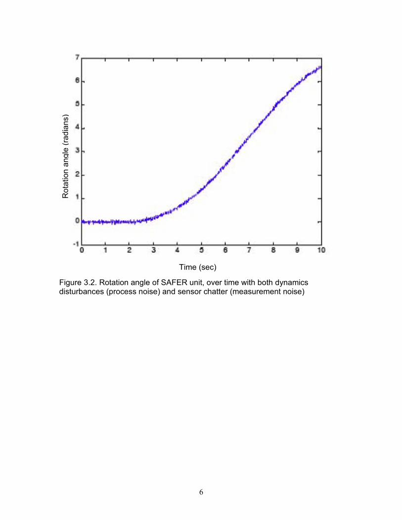
After adding process noise and measurement noise into the Simulink model, we find a set of data that is less useful than the original ideal situation of Problem 2.
Y-
i(m
)
X- i (m)
Pos
iton
Posit on
Figure 3.1 XY-position measurement of SAFER unit, with both dynamics disturbances (process noise) and sensor chatter (measurement noise)
5
Ti (
il
i
me sec)
Rot
aton
ang
e (ra
dan
s)
Figure 3.2. Rotation angle of SAFER unit, over time with both dynamics disturbances (process noise) and sensor chatter (measurement noise)
6
Problem 6.
To determine the matrices needed to create the Kalman filter, we want our dynamics to be represented in the form
!
˙ x = Ax + Bu , which is equivalent to:
We will also need to determine the measurement matrix, H; the measurement covariance matrix, R; the continuous process noise covariance matrix, Q; the initial state covariance matrix estimate, P; and the initial state vector estimate, X.
The measurement update and time update of the Kalman filter will be carried out according to the following matrix equations (Ferguson, 2006, SBE Dynamics Lecture Notes):
We must put these into Matlab form, in a discrete time-step loop. To apply the Kalman filter to our simulated noisy data, we can use the following Matlab code:
7
% Clean up the environmentclose allclear all
% Constantsrad2deg = 180/pi;deg2rad = pi/180;
% Set the time vectorstart_time = 0;stop_time = 10;time_step = 0.01;time_vec = start_time:time_step:stop_time;
% Force and torque valueson_force_val = 10;on_torque_val = 3;
% Mass propertiesmass = 125; % kginertia = 10;
% Buid the force and torque vectors as functions of timex_forcev = zeros(size(time_vec));y_forcev = zeros(size(time_vec));torquev = zeros(size(time_vec));for i = 1:length(time_vec)
if (time_vec(i) >= 7)x_forcev(i) = x_forcev(i) + on_force_val;
% Format the forces and torques for use with the source block torque = [time_vec' torquev']; x_force = [time_vec' x_forcev']; y_force = [time_vec' y_forcev'];
% Process noise variances % Note that these are squares of standard deviations, so they look pretty % small
8
pos_proc_var = 0.01;ang_proc_var = 0.001;
% Measurement noise variances% Note that these are squares of standard deviations, so they look pretty% smallpos_meas_var = 0.005;ang_meas_var = 0.001;
% Run the dynamics from the Simulink model% Check the simulation configuration dialog of the model to ensure that the% following things are set:%% Start time: start_time% Stop time: stop_time% Type: Fixed-step% Solver: ode3(Bogacki-Sharnpine)% Periodic sample time constraint: Unconstrained% Fixed-step size (fundamental sample time): time_step% Tasking mode for periodic sample times: Auto% Higher priority value indicates higher task priority: Unchecked% Automatically handle data transfers between tasks: Unchecked%% After running the simulation, the following variables are available:%% truth% meas%% Both are structures that contain the data we're interested in% The structure is automatically created by Simulink and is needlessly% complicated ... They are extracted below for simplicitysim(‘your_simulink_model’)
% Extract the truth and the measurements from the Simulink data structuresmeas_vecs = meas.signals.values;truth_vecs = truth.signals.values;
% We now proceed with the setup of the Kalman Filter% We assume that the state we want to estimate takes the following form:% X = [x y theta x_dot y_dot theta_dot]'%% The measurement vector has the following form:% y = [x_hat y_hat theta_hat]
% Form the measurement covariance matrixR = diag([pos_meas_var; pos_meas_var; ang_meas_var]);
% Form the continuous process noise covariance matrix% Note that process noise is only added to the velocity states because% we're really adding this to the state equation:%% X_dot = Phi*X + B*u + QQ = diag([0, 0, 0, pos_proc_var, pos_proc_var, ang_proc_var]);
% Put the input vectors into a matrix for easy useinput_vectors = [x_forcev', y_forcev', torquev'];
9
% Form the measurement matrix such that % y = H*X H = [1 0 0 0 0 0;
0 1 0 0 0 0; 0 0 1 0 0 0];
% Form the continuous dynamics matrix A = [0 0 0 1 0 0;
% The continuous B matrix for X_dot = AX + Bu depends on the state (angle)% So, it needs to be computed at every time step
% Define the initial error variances on the estimate we start withinit_pos_err_var = 0.025;init_vel_err_var = 1;init_ang_err_var = 0.01;init_ang_rate_err_var = 0.02;
% Initialize the state covariance estimateP_init = diag([init_pos_err_var, init_pos_err_var, init_ang_err_var, init_vel_err_var, init_vel_err_var,init_ang_rate_err_var]);P = P_init
% Initialize the state estimateX_init = truth_vecs(1,:)' + sqrtm(P)*randn(6,1);X = X_init;
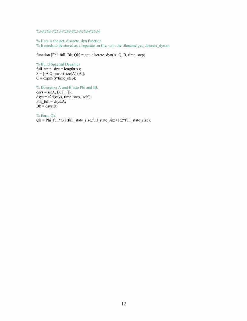
% Discretize A and B into Phi and Bkcsys = ss(A, B, [], []);dsys = c2d(csys, time_step, 'zoh');Phi_full = dsys.A;Bk = dsys.B;
% Form QkQk = Phi_full*C(1:full_state_size,full_state_size+1:2*full_state_size);
12
Problem 7.
To create the plots of estimation error and covariance bounds, we can use the following Matlab code.
% Make some plots% The truth positionfigureplot(truth_vecs(:,1), truth_vecs(:,2))gridtitle('Subject motion in X-Y plane')xlabel('X position (m)');ylabel('Y position (m)');
% The truth anglefigureplot(time_vec, truth_vecs(:,3).*rad2deg)gridtitle('Subject rotation angle')xlabel('Time (s)');ylabel('Rotation angle (degrees)');
% Position estimation errors and covariance boundsfiguresubplot(3,1,1)plot(time_vec, X_diff(1,:), time_vec, sqrt(Pdiag_store(1,:)), 'k--', time_vec, -sqrt(Pdiag_store(1,:)), 'k--')title('Position Estimation Errors and Covariance Bounds');ylabel('X Position (m)');gridsubplot(3,1,2)plot(time_vec, X_diff(2,:), time_vec, sqrt(Pdiag_store(2,:)), 'k--', time_vec, -sqrt(Pdiag_store(2,:)), 'k--')ylabel('Y Position (m)');xlabel('Time (s)')gridsubplot(3,1,3)plot(time_vec, X_diff(3,:).*rad2deg, time_vec, sqrt(Pdiag_store(3,:)).*rad2deg, 'k--', time_vec, -sqrt(Pdiag_store(3,:)).*rad2deg, 'k--')ylabel('Rotation Angle (degrees)');xlabel('Time (s)')grid
The error in our position estimation and its covariance bounds are shown in Figure 7.1.
0 1 2 3 4 5 6 7 8 9 10-0.1
-0.05
0
0.05
0.1
Position Estimation Errors and Covariance Bounds
X Position (m)
0 1 2 3 4 5 6 7 8 9 10-0.1
-0.05
0
0.05
0.1
Y Position (m)
Time (s)
0 1 2 3 4 5 6 7 8 9 10-2
-1
0
1
2
Rotation Angle (degrees)
Time (s)
Figure 7.1 Position estimation errors and covariance bounds
14
The error in our velocity estimation and its covariance bounds are shown in Figure 7-2.
0 1 2 3 4 5 6 7 8 9 10-1.5
-1
-0.5
0
0.5
1
1.5Velocity Estimation Errors and Covariance Bounds
X Velocity (m/s)
0 1 2 3 4 5 6 7 8 9 10-1.5
-1
-0.5
0
0.5
1
1.5
Y Velocity (m/s)
Time (s)
0 1 2 3 4 5 6 7 8 9 10-10
-5
0
5
10
Rotation Rate (degrees/s)
Time (s)
Figure 7.2 Velocity estimation errors and covariance bounds
15
Problem 8.
If you suspect that the friction has a Gaussian white noise effect, increase the velocity elements of the Q matrix to be at least as big as you think the friction might be. If you don't have any idea what the friction might look like, you would probably just assume it was Gaussian so that you could do the above.
If you knew exactly what the friction was, you could model it and incorporate it into the dynamics as part of the A matrix.
However, if you suspected a particular form of the friction, but did NOT know the parameters, you could “augment” the state matrix, which means incorporating the B matrix into your state vector. For instance, maybe you know that it took the form of:
F_friction = -B * velocity
But you did not know what B was. The Kalman filter has the ability to estimate what B is based on the data. The way you would do this would be to include B into your state vector as a constant. The dynamics of B are nothing (because it is constant). You would need to incorporate this state into the measurement equation (so into H) also. This way, not only would your filter track the position and velocity of the astronaut on the SAFER unit, you would also be able to do some system ID too!
16
An Introduction to the Kalman FilterGreg Welch and Gary Bishop
Updated: Monday, April 5, 2004
Abstract In 1960, R.E. Kalman published his famous paper describing a recursive solutionto the discrete-data linear filtering problem. Since that time, due in large part to advances in digital computing, the Kalman filter has been the subject of extensive research and application, particularly in the area of autonomous or assistednavigation. The Kalman filter is a set of mathematical equations that provides an efficient computational (recursive) means to estimate the state of a process, in a way that minimizes the mean of the squared error. The filter is very powerful in several aspects:it supports estimations of past, present, and even future states, and it can do so evenwhen the precise nature of the modeled system is unknown. The purpose of this paper is to provide a practical introduction to the discrete Kalman filter. This introduction includes a description and some discussion of the basicdiscrete Kalman filter, a derivation, description and some discussion of the extended Kalman filter, and a relatively simple (tangible) example with real numbers &results.
2 Welch & Bishop, An Introduction to the Kalman Filter
- -
1 The Discrete Kalman Filter In 1960, R.E. Kalman published his famous paper describing a recursive solution to the discrete-data linear filtering problem [Kalman60]. Since that time, due in large part to advances in digitalcomputing, the Kalman filter has been the subject of extensive research and application,particularly in the area of autonomous or assisted navigation. A very “friendly” introduction to thegeneral idea of the Kalman filter can be found in Chapter 1 of [Maybeck79], while a more completeintroductory discussion can be found in [Sorenson70], which also contains some interestinghistorical narrative. More extensive references include [Gelb74; Grewal93; Maybeck79; Lewis86;Brown92; Jacobs93]. The Process to be Estimated The Kalman filter addresses the general problem of trying to estimate the state x ∈ ℜn of adiscrete-time controlled process that is governed by the linear stochastic difference equation
xk = Axk 1 – + Buk 1 – + wk 1 – , (1.1)
with a measurement z ∈ ℜm that is zk = H xk + vk . (1.2)
The random variables wk and vk represent the process and measurement noise (respectively).They are assumed to be independent (of each other), white, and with normal probabilitydistributions
p w( ) ∼ N (0, Q) , (1.3) p v( ) ∼ N (0, R) . (1.4)
In practice, the process noise covariance Q and measurement noise covariance R matrices mightchange with each time step or measurement, however here we assume they are constant.
×The n n matrix A in the difference equation (1.1) relates the state at the previous time step k 1 – to the state at the current step , in the absence of either a driving function or process noise. Note k that in practice A might change with each time step, but here we assume it is constant. The n l×l ×matrix B relates the optional control input u ∈ ℜ to the state x. The m n matrix H in themeasurement equation (1.2) relates the state to the measurement zk. In practice H might changewith each time step or measurement, but here we assume it is constant. The Computational Origins of the Filter
-We define x k ∈ ℜn (note the “super minus”) to be our a priori state estimate at step k givenknowledge of the process prior to step k, and x k ∈ ℜn to be our a posteriori state estimate at stepk given measurement zk . We can then define a priori and a posteriori estimate errors as
ek ≡ xk – xk, and ek ≡ xk – xk.
3 Welch & Bishop, An Introduction to the Kalman Filter
- -
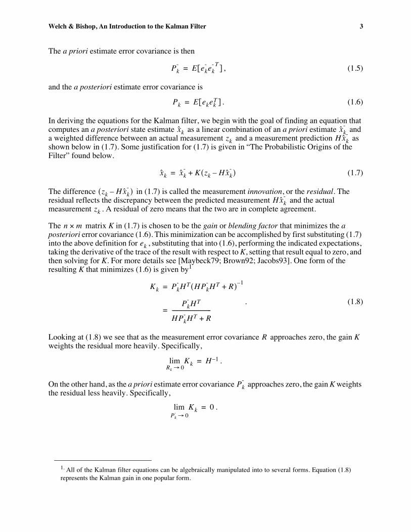
The a priori estimate error covariance is then - - - T ] ,Pk = E ekek (1.5)[
and the a posteriori estimate error covariance is Pk = E ekekT ] . (1.6)[
In deriving the equations for the Kalman filter, we begin with the goal of finding an equation that-computes an a posteriori state estimate x k as a linear combination of an a priori estimate x k and-a weighted difference between an actual measurement zk and a measurement prediction H x k asshown below in (1.7). Some justification for (1.7) is given in “The Probabilistic Origins of theFilter” found below.
xk = xk + K zk – H xk ) (1.7)( -The difference (zk – H xk ) in (1.7) is called the measurement innovation, or the residual. The-residual reflects the discrepancy between the predicted measurement H x k and the actual
measurement zk . A residual of zero means that the two are in complete agreement. The n m matrix K in (1.7) is chosen to be the gain or blending factor that minimizes the a× posteriori error covariance (1.6). This minimization can be accomplished by first substituting (1.7)into the above definition for ek , substituting that into (1.6), performing the indicated expectations,taking the derivative of the trace of the result with respect to K, setting that result equal to zero, andthen solving for K. For more details see [Maybeck79; Brown92; Jacobs93]. One form of theresulting K that minimizes (1.6) is given by1
- - 1–Kk = PkHT (HPkHT + R)- . (1.8)PkHT
= -----------------------------HPkHT + R
Looking at (1.8) we see that as the measurement error covariance R approaches zero, the gain Kweights the residual more heavily. Specifically,
H 1–lim Kk = .Rk → 0
-On the other hand, as the a priori estimate error covariance Pk approaches zero, the gain K weightsthe residual less heavily. Specifically,
lim Kk = 0 . -Pk → 0
1. All of the Kalman filter equations can be algebraically manipulated into to several forms. Equation (1.8)represents the Kalman gain in one popular form.
4 Welch & Bishop, An Introduction to the Kalman Filter
Another way of thinking about the weighting by K is that as the measurement error covariance R approaches zero, the actual measurement zk is “trusted” more and more, while the predicted-measurement H x k is trusted less and less. On the other hand, as the a priori estimate error-covariance Pk approaches zero the actual measurement zk is trusted less and less, while the-predicted measurement H x k is trusted more and more. The Probabilistic Origins of the Filter
-The justification for (1.7) is rooted in the probability of the a priori estimate x k conditioned on allprior measurements zk (Bayes’ rule). For now let it suffice to point out that the Kalman filtermaintains the first two moments of the state distribution,
E xk[ ] = xk [(E xk – xk )(xk – xk )T ] = Pk.
The a posteriori state estimate (1.7) reflects the mean (the first moment) of the state distribution— it is normally distributed if the conditions of (1.3) and (1.4) are met. The a posteriori estimate errorcovariance (1.6) reflects the variance of the state distribution (the second non-central moment). In other words,
(p xk zk ) ∼ N E xk [(( [ ], E xk – xk )(xk – xk )T ]) ( ˆ= N xk, Pk ). .
For more details on the probabilistic origins of the Kalman filter, see [Maybeck79; Brown92;Jacobs93]. The Discrete Kalman Filter Algorithm We will begin this section with a broad overview, covering the “high-level” operation of one formof the discrete Kalman filter (see the previous footnote). After presenting this high-level view, wewill narrow the focus to the specific equations and their use in this version of the filter. The Kalman filter estimates a process by using a form of feedback control: the filter estimates theprocess state at some time and then obtains feedback in the form of (noisy) measurements. As such,the equations for the Kalman filter fall into two groups: time update equations and measurement update equations. The time update equations are responsible for projecting forward (in time) thecurrent state and error covariance estimates to obtain the a priori estimates for the next time step.The measurement update equations are responsible for the feedback—i.e. for incorporating a newmeasurement into the a priori estimate to obtain an improved a posteriori estimate. The time update equations can also be thought of as predictor equations, while the measurementupdate equations can be thought of as corrector equations. Indeed the final estimation algorithmresembles that of a predictor-corrector algorithm for solving numerical problems as shown belowin Figure 1-1.
5 Welch & Bishop, An Introduction to the Kalman Filter
- -
(“Predict”) Measurement Update
(“Correct”)Time Update
Figure 1-1. The ongoing discrete Kalman filter cycle. The time updateprojects the current state estimate ahead in time. The measurement updateadjusts the projected estimate by an actual measurement at that time.
The specific equations for the time and measurement updates are presented below in Table 1-1 and Table 1-2.
Again notice how the time update equations in Table 1-1 project the state and covariance estimates forward from time step k 1 – to step k . A and B are from (1.1), while Q is from (1.3). Initialconditions for the filter are discussed in the earlier references.
xk = xk + Kk (zk – H xk ) (1.12) -–Pk = (I KkH )Pk (1.13)
The first task during the measurement update is to compute the Kalman gain, K k . Notice that the equation given here as (1.11) is the same as (1.8). The next step is to actually measure the process to obtain zk , and then to generate an a posteriori state estimate by incorporating the measurementas in (1.12). Again (1.12) is simply (1.7) repeated here for completeness. The final step is to obtain an a posteriori error covariance estimate via (1.13). After each time and measurement update pair, the process is repeated with the previous a posterioriestimates used to project or predict the new a priori estimates. This recursive nature is one of the very appealing features of the Kalman filter—it makes practical implementations much morefeasible than (for example) an implementation of a Wiener filter [Brown92] which is designed tooperate on all of the data directly for each estimate. The Kalman filter instead recursivelyconditions the current estimate on all of the past measurements. Figure 1-2 below offers a complete picture of the operation of the filter, combining the high-level diagram of Figure 1-1 with theequations from Table 1-1 and Table 1-2.
6 Welch & Bishop, An Introduction to the Kalman Filter
Filter Parameters and Tuning In the actual implementation of the filter, the measurement noise covariance R prior to operation of the filter. Measuring the measurement error covariance R
is usually measuredis generally
practical (possible) because we need to be able to measure the process anyway (while operating thefilter) so we should generally be able to take some off-line sample measurements in order todetermine the variance of the measurement noise. The determination of the process noise covariance Q is generally more difficult as we typically donot have the ability to directly observe the process we are estimating. Sometimes a relativelysimple (poor) process model can produce acceptable results if one “injects” enough uncertaintyinto the process via the selection of Q . Certainly in this case one would hope that the processmeasurements are reliable. In either case, whether or not we have a rational basis for choosing the parameters, often timessuperior filter performance (statistically speaking) can be obtained by tuning the filter parametersQ and R . The tuning is usually performed off-line, frequently with the help of another (distinct)Kalman filter in a process generally referred to as system identification.
Kk Pk - HT HPk
- HT R+( )=
x kInitial estimates for and Pk
x k x k - Kk zk H x k
-–( )+= (2) Update estimate with measurement zk
Pk I KkH–( )Pk -=
(1) Project the state ahead x k
- Ax k Buk+=
Pk - APk AT Q+=
1 – (1) Compute the Kalman gain
1 – 1 –
(3) Update the error covariance
Measurement Update (“Correct”)
(2) Project the error covariance ahead
Time Update (“Predict”)
1 – 1 –
1 –
Figure 1-2. A complete picture of the operation of the Kalman filter, combining the high-level diagram of Figure 1-1 with the equations fromTable 1-1 and Table 1-2.
In closing we note that under conditions where Q and R .are in fact constant, both the estimationerror covariance Pk and the Kalman gain Kk will stabilize quickly and then remain constant (seethe filter update equations in Figure 1-2). If this is the case, these parameters can be pre-computed by either running the filter off-line, or for example by determining the steady-state value of Pk as described in [Grewal93].
7 Welch & Bishop, An Introduction to the Kalman Filter
2
It is frequently the case however that the measurement error (in particular) does not remainconstant. For example, when sighting beacons in our optoelectronic tracker ceiling panels, thenoise in measurements of nearby beacons will be smaller than that in far-away beacons. Also, theprocess noise Q is sometimes changed dynamically during filter operation—becoming Qk —in order to adjust to different dynamics. For example, in the case of tracking the head of a user of a3D virtual environment we might reduce the magnitude of Qk if the user seems to be movingslowly, and increase the magnitude if the dynamics start changing rapidly. In such cases Qk mightbe chosen to account for both uncertainty about the user’s intentions and uncertainty in the model.
The Extended Kalman Filter (EKF) The Process to be Estimated As described above in section 1, the Kalman filter addresses the general problem of trying toestimate the state x ∈ ℜn of a discrete-time controlled process that is governed by a linearstochastic difference equation. But what happens if the process to be estimated and (or) themeasurement relationship to the process is non-linear? Some of the most interesting and successfulapplications of Kalman filtering have been such situations. A Kalman filter that linearizes aboutthe current mean and covariance is referred to as an extended Kalman filter or EKF. In something akin to a Taylor series, we can linearize the estimation around the current estimateusing the partial derivatives of the process and measurement functions to compute estimates evenin the face of non-linear relationships. To do so, we must begin by modifying some of the materialpresented in section 1. Let us assume that our process again has a state vector x ∈ ℜn , but that theprocess is now governed by the non-linear stochastic difference equation
xk = f xk 1 – , uk 1 – , wk 1 – ) , (2.1)( with a measurement z ∈ ℜm that is
zk = h xk, vk ) , (2.2)( where the random variables wk and vk again represent the process and measurement noise as in(1.3) and (1.4). In this case the non-linear function f in the difference equation (2.1) relates thestate at the previous time step k 1 – to the state at the current time step . It includes as parameters kany driving function uk 1 – and the zero-mean process noise wk. The non-linear function h in themeasurement equation (2.2) relates the state xk to the measurement zk . In practice of course one does not know the individual values of the noise wk and vk at each timestep. However, one can approximate the state and measurement vector without them as
xk = ( ,f xk 1 – uk 1 – , 0) (2.3)
and zk = h x( ˜ k, 0) , (2.4)
where x k is some a posteriori estimate of the state (from a previous time step k).
8 Welch & Bishop, An Introduction to the Kalman Filter
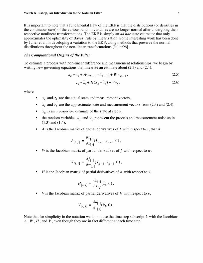
It is important to note that a fundamental flaw of the EKF is that the distributions (or densities inthe continuous case) of the various random variables are no longer normal after undergoing theirrespective nonlinear transformations. The EKF is simply an ad hoc state estimator that onlyapproximates the optimality of Bayes’ rule by linearization. Some interesting work has been doneby Julier et al. in developing a variation to the EKF, using methods that preserve the normaldistributions throughout the non-linear transformations [Julier96]. The Computational Origins of the Filter To estimate a process with non-linear difference and measurement relationships, we begin bywriting new governing equations that linearize an estimate about (2.3) and (2.4),
xk ≈ xk + A xk 1 – – xk 1 – ) + W wk 1 – , (2.5)( (zk ≈ zk + H xk – xk) + V vk . (2.6)
where • xk and zk are the actual state and measurement vectors, • xk and zk are the approximate state and measurement vectors from (2.3) and (2.4), • x k is an a posteriori estimate of the state at step k, • the random variables wk and vk represent the process and measurement noise as in
(1.3) and (1.4). • A is the Jacobian matrix of partial derivatives of f with respect to x, that is
∂ f [ ] x= xij
( ˆ k 1 – , uk 1 – , 0) ,,A[i j] ∂ [ ] • W is the Jacobian matrix of partial derivatives of f with respect to w,
∂ f [ ] xi,W [i j] = ∂ [ ]
( ˆ k 1 – , uk 1 – , 0) ,w j• H is the Jacobian matrix of partial derivatives of h with respect to x,
∂h[ ] xiH [i j] = ∂ [ ]( ˜ k, 0) ,, x j
• V is the Jacobian matrix of partial derivatives of h with respect to v, ∂h[ ] x= v
ij
( ˜ k, 0) .,V [i j] ∂ [ ]
Note that for simplicity in the notation we do not use the time step subscript k with the Jacobians A , W , H , and V , even though they are in fact different at each time step.
9 Welch & Bishop, An Introduction to the Kalman Filter
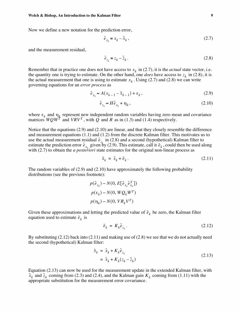
Now we define a new notation for the prediction error, exk
≡ xk – xk , (2.7)
and the measurement residual, ezk
≡ zk – zk . (2.8)
Remember that in practice one does not have access to xk in (2.7), it is the actual state vector, i.e.the quantity one is trying to estimate. On the other hand, one does have access to zk in (2.8), it isthe actual measurement that one is using to estimate xk . Using (2.7) and (2.8) we can writegoverning equations for an error process as
exk ≈ A xk 1 – – xk 1 – ) εk , (2.9)( +
ezk ≈ Hexk
+ ηk , (2.10)
where εk and ηk represent new independent random variables having zero mean and covariancematrices WQW T and VRV T , with Q and R as in (1.3) and (1.4) respectively. Notice that the equations (2.9) and (2.10) are linear, and that they closely resemble the difference and measurement equations (1.1) and (1.2) from the discrete Kalman filter. This motivates us touse the actual measurement residual ezk
in (2.8) and a second (hypothetical) Kalman filter toestimate the prediction error e given by (2.9). This estimate, call it ek , could then be used alongxkwith (2.7) to obtain the a posteriori state estimates for the original non-linear process as
xk = xk + ek . (2.11)
The random variables of (2.9) and (2.10) have approximately the following probabilitydistributions (see the previous footnote):
( ˜ [ ˜p e ) ∼ N (0, E e eT ])xk xk xk
( ) ∼ N (0, W QkW T )p εk( ) ∼ N (0, V RkV T )p ηk
Given these approximations and letting the predicted value of ek be zero, the Kalman filterequation used to estimate ek is
ek = Kkezk. (2.12)
By substituting (2.12) back into (2.11) and making use of (2.8) we see that we do not actually need the second (hypothetical) Kalman filter:
xk = xk + ˜Kkezk
= xk + Kk(zk – zk) (2.13)
Equation (2.13) can now be used for the measurement update in the extended Kalman filter, with xk and zk coming from (2.3) and (2.4), and the Kalman gain Kk coming from (1.11) with theappropriate substitution for the measurement error covariance.
10 Welch & Bishop, An Introduction to the Kalman Filter
- -
The complete set of EKF equations is shown below in Table 2-1 and Table 2-2. Note that we have -substituted x k for x k to remain consistent with the earlier “super minus” a priori notation, and thatwe now attach the subscript k to the Jacobians A , W , H , and V , to reinforce the notion that theyare different at (and therefore must be recomputed at) each time step.
Table 2-1: EKF time update equations. - ( ˆxk = f xk 1 – , uk 1 – , 0) (2.14)
-Pk = AkPk 1 – AkT + W kQk 1 – W kT (2.15)
As with the basic discrete Kalman filter, the time update equations in Table 2-1 project the statekand covariance estimates from the previous time step k 1 – to the current time step . Again f in
(2.14) comes from (2.3), Ak and W k are the process Jacobians at step k, and Qk is the processnoise covariance (1.3) at step k.
Table 2-2: EKF measurement update equations. - - 1 – Kk = PkHkT (HkPkHkT + V kRkV kT ) (2.16)
xk = xk + Kk(zk – h xk, 0)) (2.17)( ˆ -–Pk = (I KkHk)Pk (2.18)
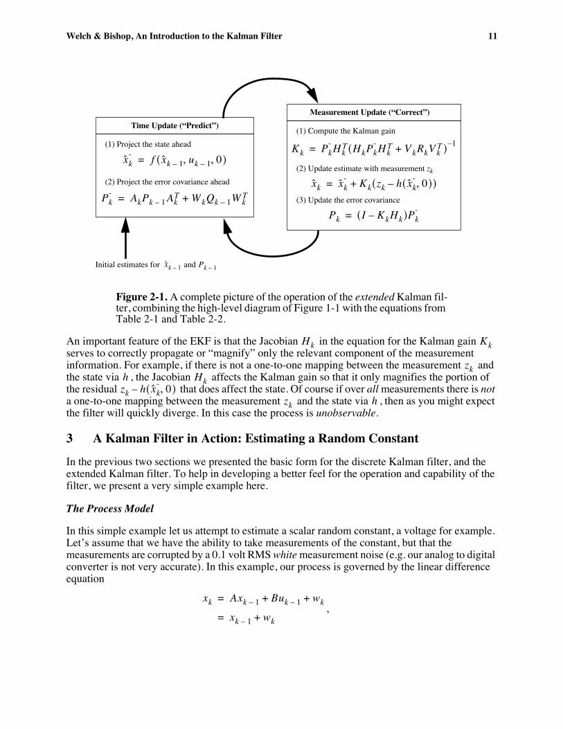
As with the basic discrete Kalman filter, the measurement update equations in Table 2-2 correctthe state and covariance estimates with the measurement zk . Again h in (2.17) comes from (2.4),Hk and V are the measurement Jacobians at step k, and Rk is the measurement noise covariance(1.4) at step k. (Note we now subscript R allowing it to change with each measurement.) The basic operation of the EKF is the same as the linear discrete Kalman filter as shown inFigure 1-1. Figure 2-1 below offers a complete picture of the operation of the EKF, combining the high-level diagram of Figure 1-1 with the equations from Table 2-1 and Table 2-2.
11 Welch & Bishop, An Introduction to the Kalman Filter
3
Kk Pk - HkT HkPk
- HkT V kRkV kT+( )=
x k x k - Kk zk h x k
- 0,( )–( )+= (2) Update estimate with measurement zk
Pk I KkHk–( )Pk -=
(1) Project the state ahead x k
- f x k uk 0, ,( )=
Pk - AkPk AkT W kQk W kT+=
x kInitial estimates for and Pk
1 – (1) Compute the Kalman gain
(3) Update the error covariance
Measurement Update (“Correct”)
(2) Project the error covariance ahead
Time Update (“Predict”)
1 – 1 –
1 – 1 –
1 – 1 –
Figure 2-1. A complete picture of the operation of the extended Kalman filter, combining the high-level diagram of Figure 1-1 with the equations from Table 2-1 and Table 2-2.
An important feature of the EKF is that the Jacobian Hk in the equation for the Kalman gain Kkserves to correctly propagate or “magnify” only the relevant component of the measurementinformation. For example, if there is not a one-to-one mapping between the measurement zk andthe state via h , the Jacobian Hk affects the Kalman gain so that it only magnifies the portion of-( ˆthe residual zk – h xk, 0) that does affect the state. Of course if over all measurements there is not a one-to-one mapping between the measurement zk and the state via h , then as you might expectthe filter will quickly diverge. In this case the process is unobservable.
A Kalman Filter in Action: Estimating a Random Constant In the previous two sections we presented the basic form for the discrete Kalman filter, and theextended Kalman filter. To help in developing a better feel for the operation and capability of thefilter, we present a very simple example here. The Process Model In this simple example let us attempt to estimate a scalar random constant, a voltage for example.Let’s assume that we have the ability to take measurements of the constant, but that themeasurements are corrupted by a 0.1 volt RMS white measurement noise (e.g. our analog to digitalconverter is not very accurate). In this example, our process is governed by the linear differenceequation
xk = + wkAxk 1 – + Buk 1 – = xk 1 – + wk
,
12 Welch & Bishop, An Introduction to the Kalman Filter
----------------
with a measurement z ∈ ℜ1 that is zk = H xk + vk
= xk + vk .
The state does not change from step to step so A = 1 . There is no control input so u = 0 . Ournoisy measurement is of the state directly so H = 1 . (Notice that we dropped the subscript k in several places because the respective parameters remain constant in our simple model.) The Filter Equations and Parameters Our time update equations are
-xk = xk 1– , -Pk = Pk 1– + Q ,
and our measurement update equations are Kk = Pk
- Pk - + R( ) 1–
= Pk - , (3.1)
Pk - + R
x k = ,x k - Kk zk x k
-–( )+
Pk = .1 Kk–( )Pk -
Presuming a very small process variance, we let Q = . (We could certainly let1e 5– Q = but0assuming a small but non-zero value gives us more flexibility in “tuning” the filter as we willdemonstrate below.) Let’s assume that from experience we know that the true value of the randomconstant has a standard normal probability distribution, so we will “seed” our filter with the guessthat the constant is 0. In other words, before starting we let x k 1– = 0 . Similarly we need to choose an initial value for Pk 1– , call it P0 . If we were absolutely certain thatour initial state estimate x 0 = 0 was correct, we would let P0 = 0 . However given theuncertainty in our initial estimate x 0 , choosing P0 = 0 would cause the filter to initially andalways believe x k = 0 . As it turns out, the alternative choice is not critical. We could choosealmost any P0 ≠ 0 and the filter would eventually converge. We’ll start our filter with P0 = 1 .
13 Welch & Bishop, An Introduction to the Kalman Filter
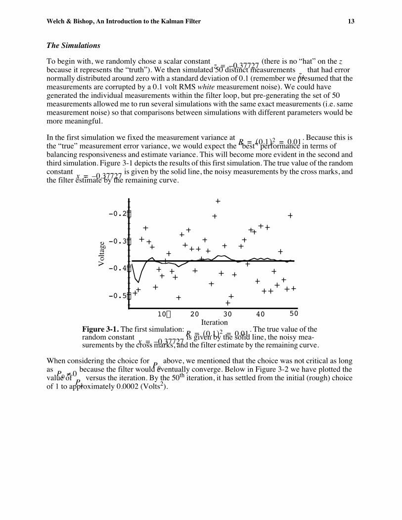
The Simulations To begin with, we randomly chose a scalar constant (there is no “hat” on the zz = 0.37727 – because it represents the “truth”). We then simulated 50 distinct measurements zk
that had error normally distributed around zero with a standard deviation of 0.1 (remember we presumed that themeasurements are corrupted by a 0.1 volt RMS white measurement noise). We could havegenerated the individual measurements within the filter loop, but pre-generating the set of 50measurements allowed me to run several simulations with the same exact measurements (i.e. samemeasurement noise) so that comparisons between simulations with different parameters would bemore meaningful. In the first simulation we fixed the measurement variance at R = (0.1)2 = 0.01. Because this isthe “true” measurement error variance, we would expect the “best” performance in terms ofbalancing responsiveness and estimate variance. This will become more evident in the second andthird simulation. Figure 3-1 depicts the results of this first simulation. The true value of the random
is given by the solid line, the noisy measurements by the cross marks, andconstant x = 0.37727 – the filter estimate by the remaining curve.
Figure 3-1. The first simulation: . The true value of therandom constant is given by the solid line, the noisy measurements by the cross marks, and the filter estimate by the remaining curve.
5040302010
-0.2
-0.3
-0.4
-0.5
Iteration
Volta
ge
R 0.1( )2 0.01= = x = 0.37727 –
When considering the choice for P0 above, we mentioned that the choice was not critical as long
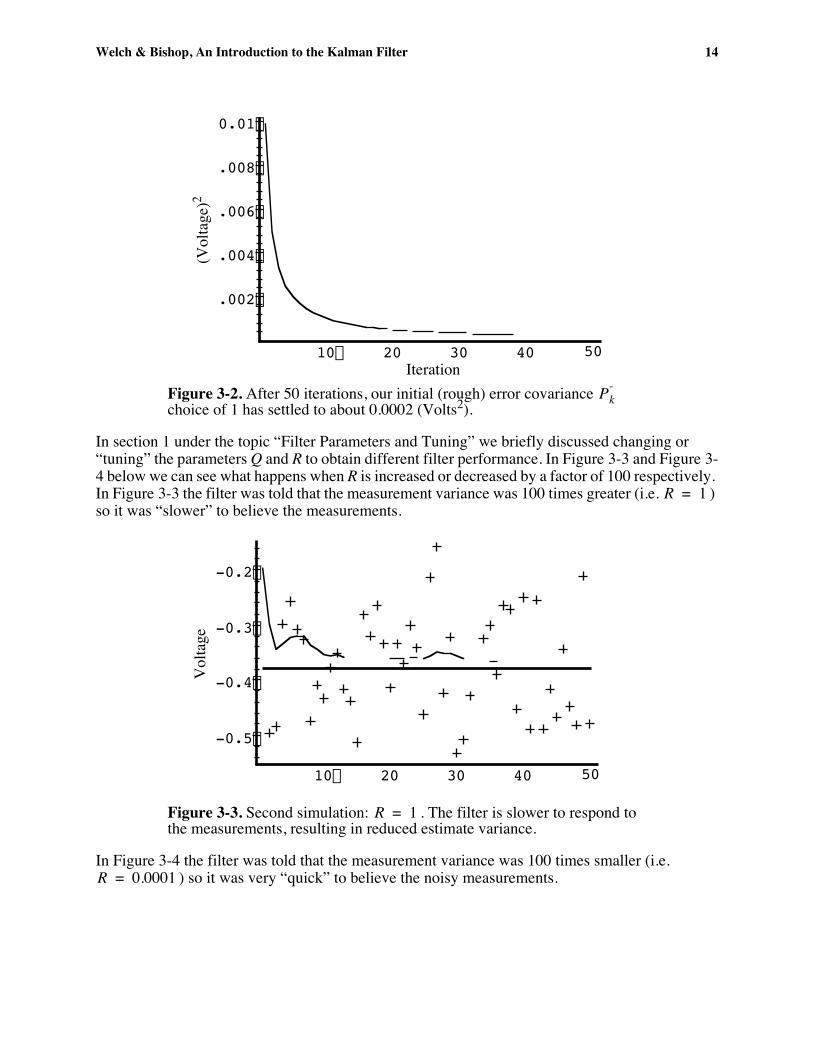
as P0 ≠ 0 because the filter would eventually converge. Below in Figure 3-2 we have plotted thevalue of versus the iteration. By the 50th iteration, it has settled from the initial (rough) choicePkof 1 to approximately 0.0002 (Volts2).
14 Welch & Bishop, An Introduction to the Kalman Filter
5040302010
0.01
0.008
0.006
0.004
0.002
Iteration
(Volt
age)2
-Figure 3-2. After 50 iterations, our initial (rough) error covariance Pkchoice of 1 has settled to about 0.0002 (Volts2). In section 1 under the topic “Filter Parameters and Tuning” we briefly discussed changing or“tuning” the parameters Q and R to obtain different filter performance. In Figure 3-3 and Figure 34 below we can see what happens when R is increased or decreased by a factor of 100 respectively.In Figure 3-3 the filter was told that the measurement variance was 100 times greater (i.e. R = 1 )so it was “slower” to believe the measurements.
5040302010
-0.2
-0.3
-0.4
-0.5
Volta
ge
Figure 3-3. Second simulation: R = 1 . The filter is slower to respond tothe measurements, resulting in reduced estimate variance.
In Figure 3-4 the filter was told that the measurement variance was 100 times smaller (i.e.R = 0.0001 ) so it was very “quick” to believe the noisy measurements.
15 Welch & Bishop, An Introduction to the Kalman Filter
5040302010
-0.2
-0.3
-0.4
-0.5
Volta
ge
Figure 3-4. Third simulation: R = 0.0001 . The filter responds to measurements quickly, increasing the estimate variance.
While the estimation of a constant is relatively straight-forward, it clearly demonstrates theworkings of the Kalman filter. In Figure 3-3 in particular the Kalman “filtering” is evident as theestimate appears considerably smoother than the noisy measurements.
16 Welch & Bishop, An Introduction to the Kalman Filter
References
Brown92 Brown, R. G. and P. Y. C. Hwang. 1992. Introduction to Random Signalsand Applied Kalman Filtering, Second Edition, John Wiley & Sons, Inc.
Gelb74 Gelb, A. 1974. Applied Optimal Estimation, MIT Press, Cambridge, MA. Grewal93 Grewal, Mohinder S., and Angus P. Andrews (1993). Kalman Filtering The
ory and Practice. Upper Saddle River, NJ USA, Prentice Hall. Jacobs93 Jacobs, O. L. R. 1993. Introduction to Control Theory, 2nd Edition. Oxford
University Press. Julier96 Julier, Simon and Jeffrey Uhlman. “A General Method of Approximating
Nonlinear Transformations of Probability Distributions,” Robotics Research Group, Department of Engineering Science, University of Oxford[cited 14 November 1995]. Available from http://www.robots.ox.ac.uk/~si-ju/work/publications/Unscented.zip. Also see: “A New Approach for Filtering Nonlinear Systems” by S. J. Julier,J. K. Uhlmann, and H. F. Durrant-Whyte, Proceedings of the 1995 Ameri-can Control Conference, Seattle, Washington, Pages:1628-1632. Availablefrom http://www.robots.ox.ac.uk/~siju/work/publications/ACC95_pr.zip. Also see Simon Julier's home page at http://www.robots.ox.ac.uk/~siju/.
Kalman60 Kalman, R. E. 1960. “A New Approach to Linear Filtering and PredictionProblems,” Transaction of the ASME—Journal of Basic Engineering,pp. 35-45 (March 1960).
Lewis86 Lewis, Richard. 1986. Optimal Estimation with an Introduction to Stochastic Control Theory, John Wiley & Sons, Inc.
Maybeck79 Maybeck, Peter S. 1979. Stochastic Models, Estimation, and Control, Volume 1, Academic Press, Inc.
Sorenson70 Sorenson, H. W. 1970. “Least-Squares estimation: from Gauss to Kalman,”IEEE Spectrum, vol. 7, pp. 63-68, July 1970.