SBS Chapter 2: Limits & continuity

(SBS 2.1) Limit of a function

Consider a free falling body with no air resistance. Fallsapproximately s(t) = 16t2 feet in t seconds.

2 We already know how to �nd the average velocityover an interval of time.

2 Now we want to know instantaneous velocity att = 2 seconds, for example. We can express this asa limit.

Compute the average velocity over a smaller and smallertime interval near t = 2 seconds.

Start with v̄ as the average velocity over the interval1.9≤ t ≤ 2.

v̄ =distance traveled

elapsed time

=s(2)− s(1.9)

2−1.9

=16(2)2−16(1.9)2

0.1= 62.4 ft/s

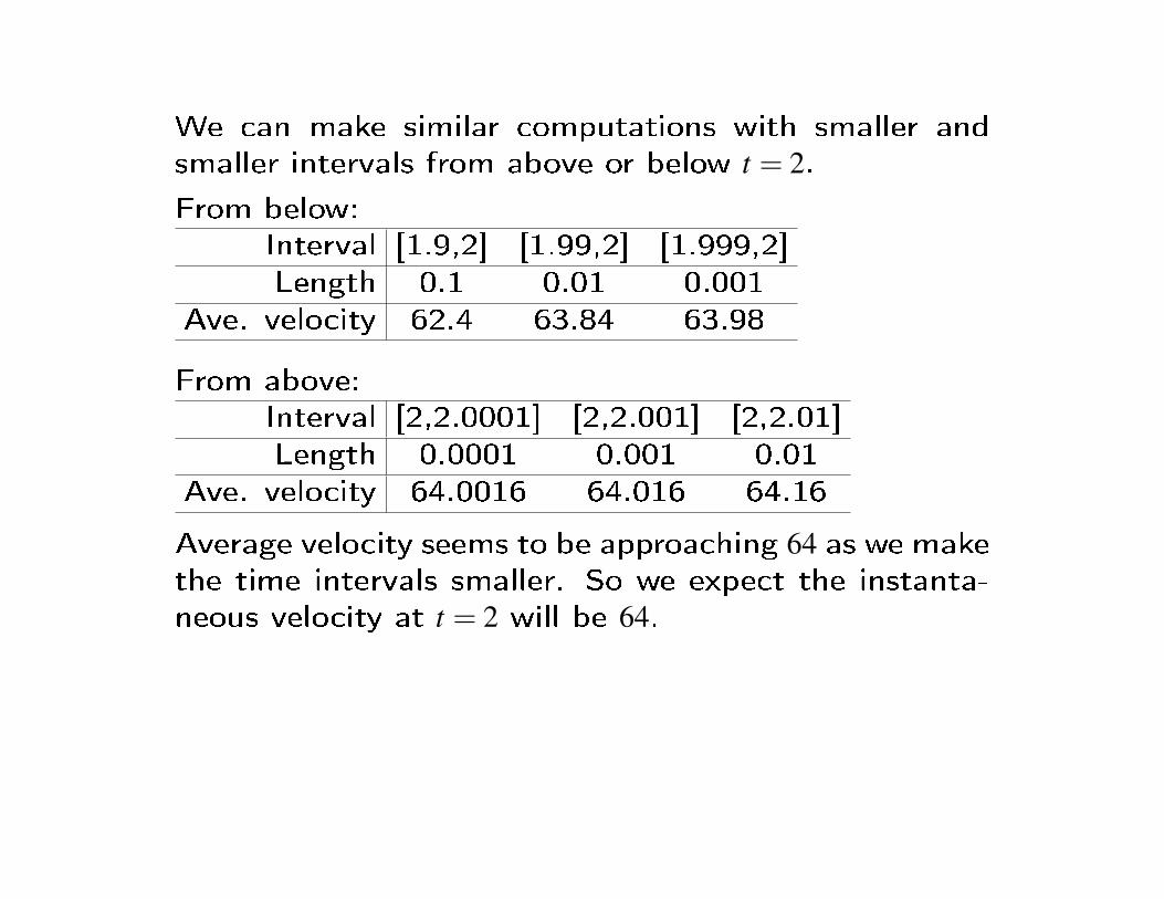
We can make similar computations with smaller andsmaller intervals from above or below t = 2.From below:

Interval [1.9,2] [1.99,2] [1.999,2]Length 0.1 0.01 0.001

Ave. velocity 62.4 63.84 63.98

From above:Interval [2,2.0001] [2,2.001] [2,2.01]Length 0.0001 0.001 0.01

Ave. velocity 64.0016 64.016 64.16

Average velocity seems to be approaching 64 as we makethe time intervals smaller. So we expect the instanta-neous velocity at t = 2 will be 64.

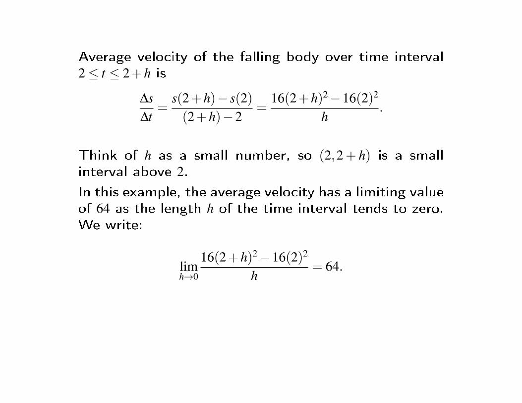
Average velocity of the falling body over time interval2≤ t ≤ 2+h is

∆s∆t

=s(2+h)− s(2)(2+h)−2

=16(2+h)2−16(2)2

h.

Think of h as a small number, so (2,2+ h) is a smallinterval above 2.In this example, the average velocity has a limiting valueof 64 as the length h of the time interval tends to zero.We write:

limh→0

16(2+h)2−16(2)2

h= 64.

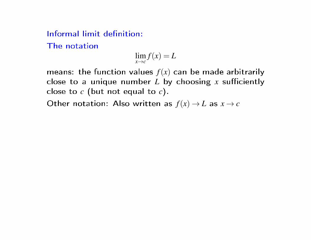
Informal limit de�nition:

The notationlimx→c

f (x) = L

means: the function values f (x) can be made arbitrarilyclose to a unique number L by choosing x su�cientlyclose to c (but not equal to c).

Other notation: Also written as f (x)→ L as x→ c

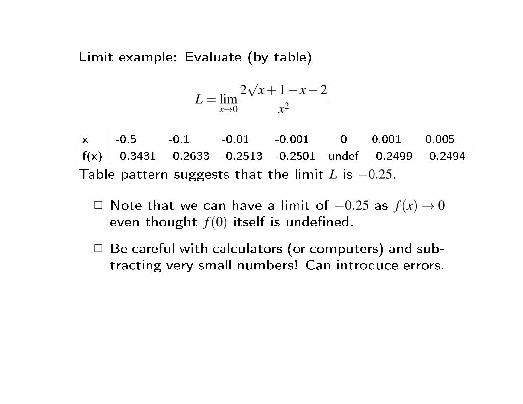
Limit example: Evaluate (by table)

L = limx→0

2√

x+1− x−2x2

x -0.5 -0.1 -0.01 -0.001 0 0.001 0.005

f(x) -0.3431 -0.2633 -0.2513 -0.2501 undef -0.2499 -0.2494

Table pattern suggests that the limit L is −0.25.

2 Note that we can have a limit of −0.25 as f (x)→ 0even thought f (0) itself is unde�ned.

2 Be careful with calculators (or computers) and sub-tracting very small numbers! Can introduce errors.

One-Sided Limits

Right-hand limit:lim

x→c+= L

if we can make f (x) arbitrarily close to L by choosing xsu�ciently close to c on a small interval (c,b) immedi-ately to the right of c.

Left-hand limit:lim

x→c−= L

if we can make f (x) arbitrarily close to L by choosing xsu�ciently close to c on a small interval (a,c) immedi-ately to the left of c.

Theorem. (One-sided limit theorem)The two-sided limit limx→c f (x) exists i� the two one-sided limits exist and are equal. Furthermore, if

limx→c−

f (x) = L = limx→c+

f (x),

thenlimx→c

f (x) = L

2 Note that the limit does not depend on how thefunction behaves exactly at c.

2 The function does not even have to be de�ned atx = c!

Example: consider 3 examples with same limit

f (x) =x2−1x−1

g(x) =

{x2−1x−1 , x 6= 11, x = 1

h(x) = x+1

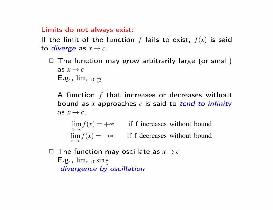
Limits do not always exist:

If the limit of the function f fails to exist, f (x) is saidto diverge as x→ c.

2 The function may grow arbitrarily large (or small)as x→ cE.g., limx→0

1x2

A function f that increases or decreases withoutbound as x approaches c is said to tend to in�nityas x→ c.

limx→c

f (x) = +∞ if f increases without bound

limx→c

f (x) =−∞ if f decreases without bound

2 The function may oscillate as x→ cE.g., limx→0 sin 1

xdivergence by oscillation

Formal de�nition of a limit (epsilon-delta de�nition):

De�nition. The limit statement:

limx→c

f (x) = L

means that for each number ε > 0 there corresponds anumber δ > 0 such that | f (x)−L|< ε whenever 0< |x−c|<δ .

In other words:

2 If the distance between x and c is small enough,then the distance between f (x) and L is also small.

2 If x is in (c,c+δ ) or (c−δ ,c), then f (x) must be inthe interval (L− ε, L+ ε).

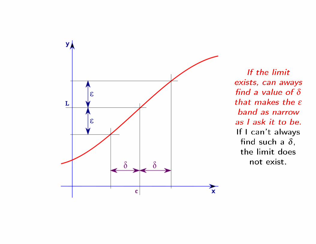
If the limitexists, can aways�nd a value of δ

that makes the ε

band as narrowas I ask it to be.If I can't always�nd such a δ ,the limit doesnot exist.

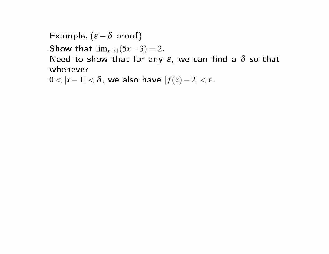
Example. (ε−δ proof)

Show that limx→1(5x−3) = 2.Need to show that for any ε, we can �nd a δ so thatwhenever0 < |x−1|< δ , we also have | f (x)−2|< ε.

Algebraic computation of limits (SBS 2.2)

Basic properties and rules for limits:

For any real number c, suppose f and g both have limitsas x→ c, and let k be a constant:

Constant rule:

limx→c

k = k

Limit of x rule:

limx→c

x = c

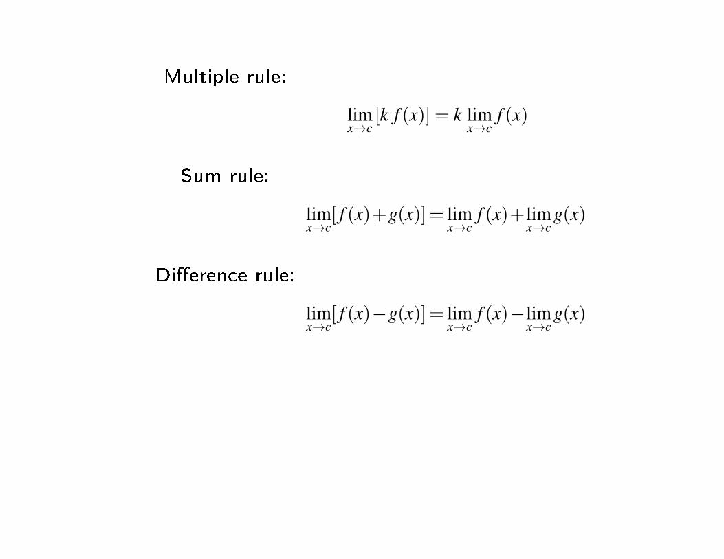
Multiple rule:

limx→c

[k f (x)] = k limx→c

f (x)

Sum rule:

limx→c

[ f (x)+g(x)]= limx→c

f (x)+limx→c

g(x)

Di�erence rule:

limx→c

[ f (x)−g(x)]= limx→c

f (x)−limx→c

g(x)

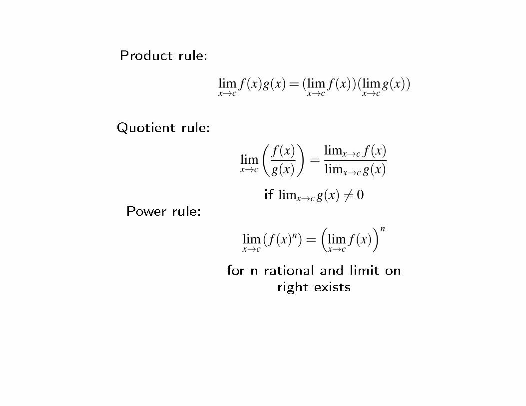
Product rule:

limx→c

f (x)g(x)= (limx→c

f (x))(limx→c

g(x))

Quotient rule:

limx→c

(f (x)g(x)

)=

limx→c f (x)limx→c g(x)

if limx→c g(x) 6= 0Power rule:

limx→c

( f (x)n) =(

limx→c

f (x))n

for n rational and limit onright exists

Limit of a polynomial:

If P is a polynomial function, then

limx→c

P(x) = P(c)

Proof: use �rst 5 rules.

Limit of a rational function:

If Q is a rational functionQ(x) = P(x)

D(x) then

limx→c

Q(x) =P(c)D(c)

provided limx→c D(x) 6= 0Proof: use Quotient Rule and Limit of a Polynomialrule.

Limits of trigonometric functions:

If c is any number in the domain of the given function,then

limx→c

(cosx) = cosc limx→c

(secx) = secc

limx→c

(sinx) = sinc limx→c

(cscx) = cscc

limx→c

(tanx) = tanc limx→c

(cotx) = cotc

Examples of limits: sometimes need to manipulate func-tion to �nd the limit

2 Fractional reduction

limx→1

x2+ x−2x2− x

Note that f (1) is unde�ned. But the limit still exists asx→ 1.

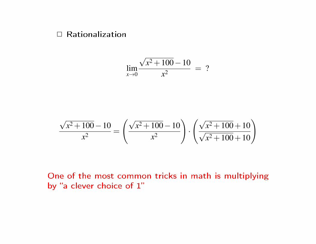
2 Rationalization

limx→0

√x2+100−10

x2 = ?

√x2+100−10

x2 =

(√x2+100−10

x2

)·

(√x2+100+10√x2+100+10

)

One of the most common tricks in math is multiplyingby �a clever choice of 1�

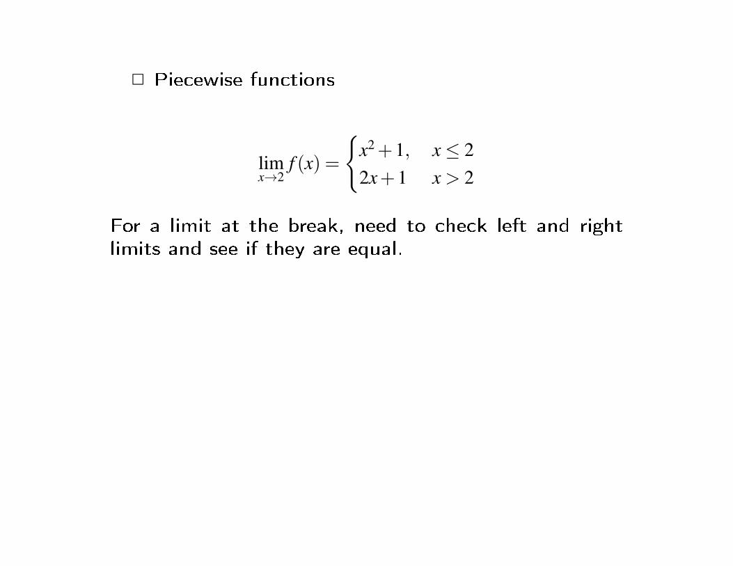
2 Piecewise functions

limx→2

f (x) =

{x2+1, x≤ 22x+1 x > 2

For a limit at the break, need to check left and rightlimits and see if they are equal.

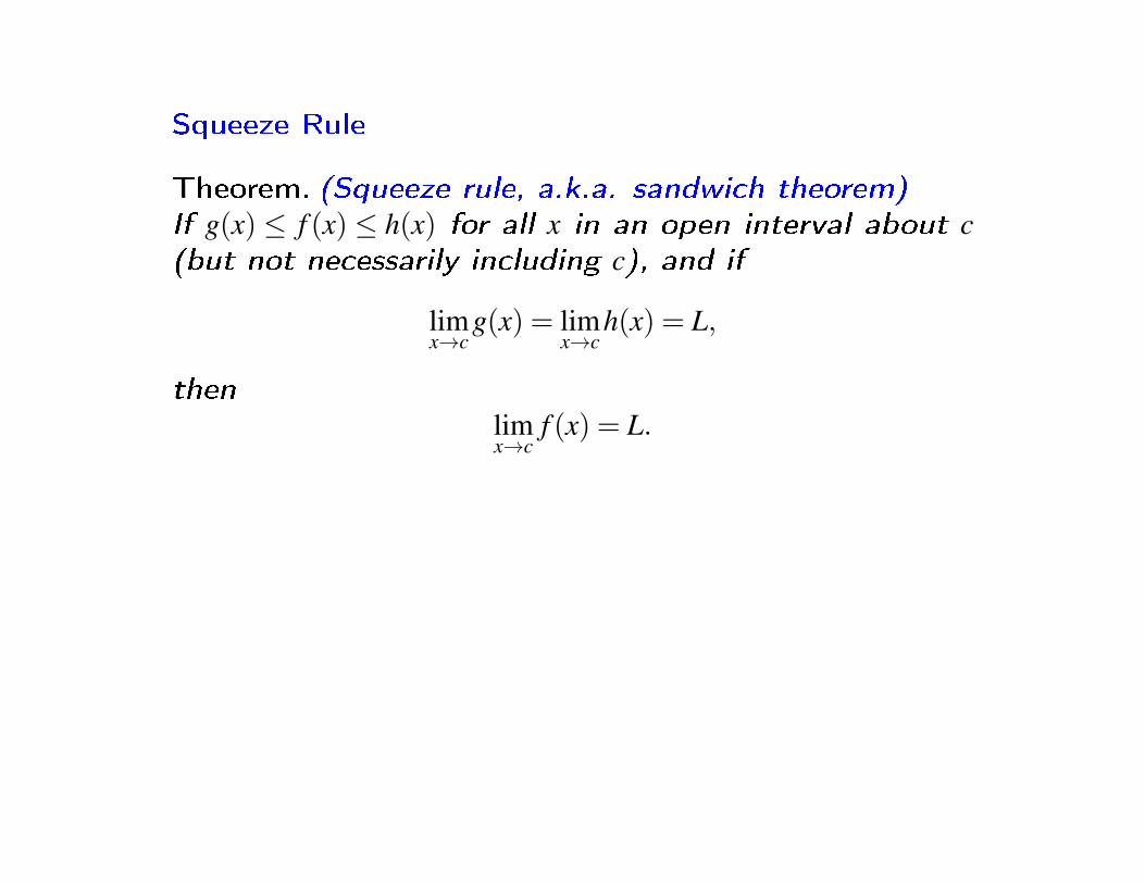
Squeeze Rule

Theorem. (Squeeze rule, a.k.a. sandwich theorem)If g(x) ≤ f (x) ≤ h(x) for all x in an open interval about c(but not necessarily including c), and if

limx→c

g(x) = limx→c

h(x) = L,

thenlimx→c

f (x) = L.

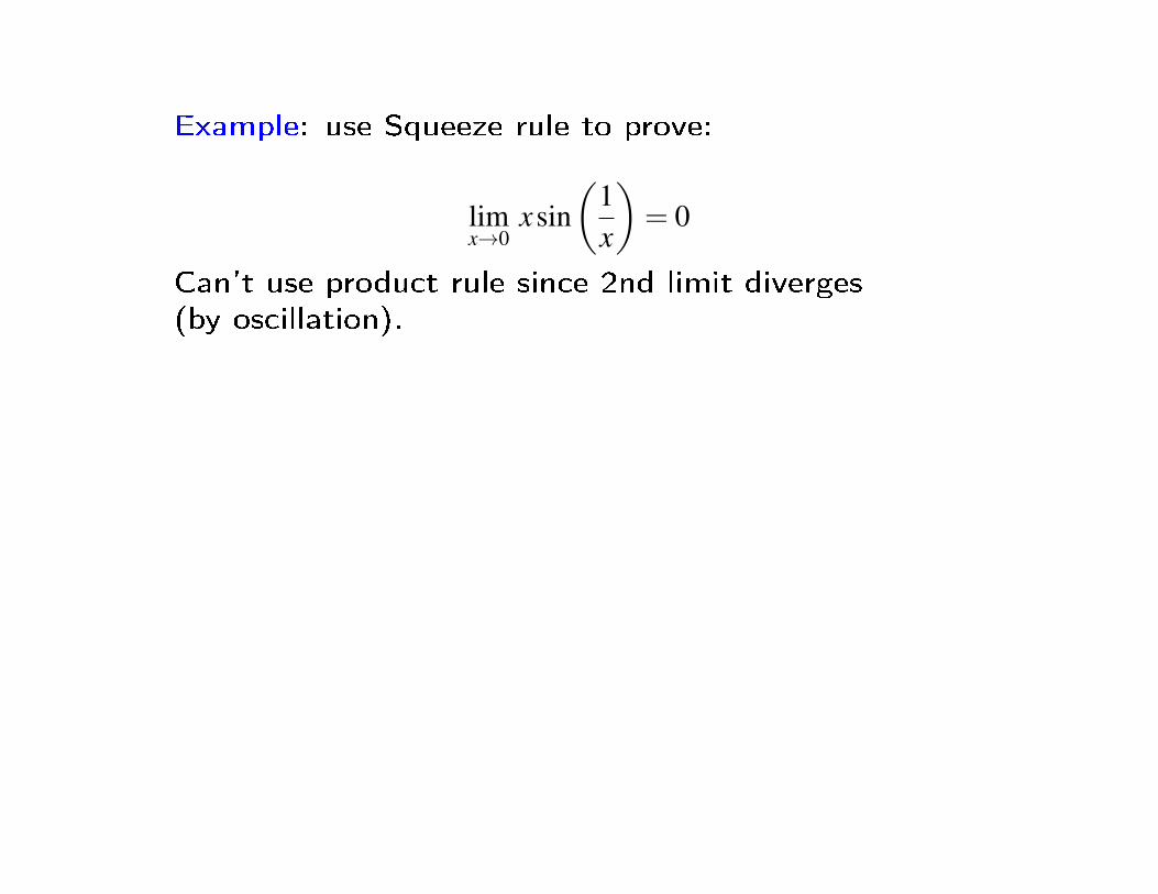
Example: use Squeeze rule to prove:

limx→0

xsin(

1x

)= 0

Can't use product rule since 2nd limit diverges(by oscillation).

For proof, recall −|a| ≤ a≤ |a| and |sin 1x| ≤ 1 for all x 6= 0:

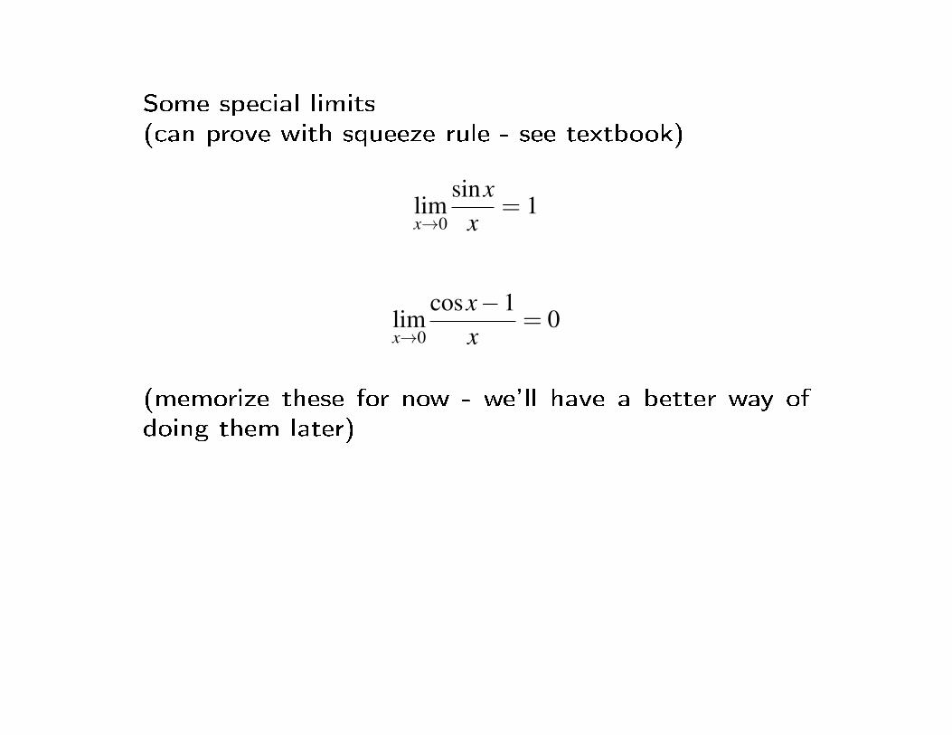
Some special limits(can prove with squeeze rule - see textbook)

limx→0

sinxx

= 1

limx→0

cosx−1x

= 0

(memorize these for now - we'll have a better way ofdoing them later)

Continuity (SBS 2.3)

Intuitively, continuity means �without jumps or breaks.�

Formal de�nition:

De�nition. A function f is continuous at a point x = c ifthe following three conditions are all satis�ed:

1. f (c) is de�ned

2. limx→c f (x) exists

3. limx→c f (x) = f (c)

A function that is not continuous at c is said to have adiscontinuity at that point.

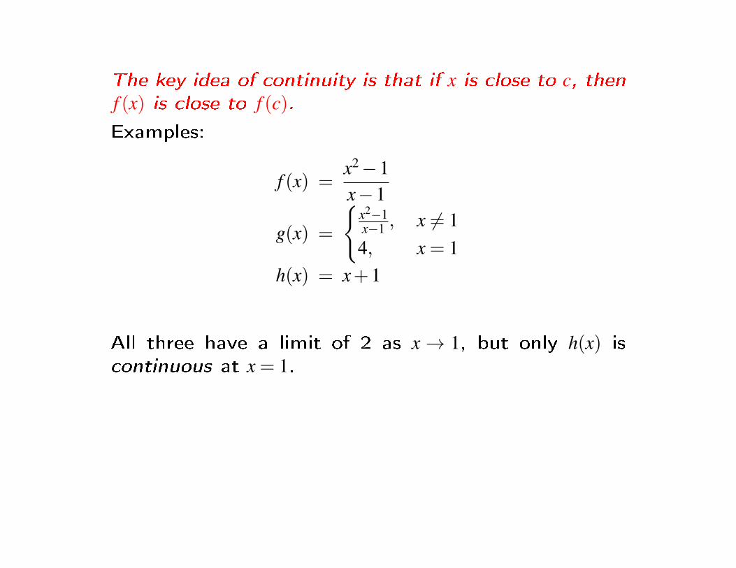
The key idea of continuity is that if x is close to c, thenf (x) is close to f (c).

Examples:

f (x) =x2−1x−1

g(x) =

{x2−1x−1 , x 6= 14, x = 1

h(x) = x+1

All three have a limit of 2 as x→ 1, but only h(x) iscontinuous at x = 1.

Some common discontinuity examples: holes, poles,jumps

2 hole:

• limx→c f (x) exists, but f (c) not de�ned

• limx→c f (x) exists, f (c) de�ned, but f (c) 6= limx→c f (x)

2 jump:

• left limit not equal to right limit

2 pole:

• f (c) de�ned, but either left or right limit →±∞

Continuity Theorem

Theorem. If f is a polynomial, rational function, powerfunction, trigonometric function, or an inverse trigono-metric function, then f is continuous at any numberx = c for which f (c) is de�ned (i.e., f is continuous ateach x in its domain).

Theorem. If functions f and g are continuous at x = c,then the following functions are also continuous at x = c:

Scalar multiple: k f (x) for any const k

Sum and di�erence: f (x)+g(x) and f (x)−g(x)

Product: f (x)g(x)

Quotient: f (x)g(x) provided g(c) 6= 0

Composition: f ◦g(x) provided g cont at cand f cont at g(c)

Theorem. (Composition Limit Rule)If limx→c g(x) = L and f is continuous at L,then limx→c f [g(x)] = f (L).I.e.,

limx→c

f [g(x)] = f[limx→c

g(x)]= f (L)

Applies similarly to left and right limits.

Idea is that the limit of a continuous function is thefunction of the limiting value.

Continuity from the left and right:

De�nition. The function f is continuous from the rightat a i�

limx→a+

f (x) = f (a)

The function f is continuous from the left at b i�

limx→b−

f (x) = f (b)

I.e., continuous from the right at a i�

1. f (a) is de�ned

2. limx→c+ f (x) exists

3. limx→c+ f (x) = f (a)

(Similarly for left continuity.)

Continuity on an interval:

De�nition. The function f is continuous on the openinterval (a,b) if it is continuous at each number in theinterval.(Note that the end points are not in the interval.)

2 If f is continuous on (a,b) and continuous from theright at a, then f is continuous on the half-openinterval [a,b).

2 If f is continuous on (a,b) and continuous from theleft at b, then f is continuous on the half-openinterval (a,b].

2 If f is continuous on (a,b), continuous from theright at a, and continuous from the left at b, thenf is continuous on the closed interval [a,b].

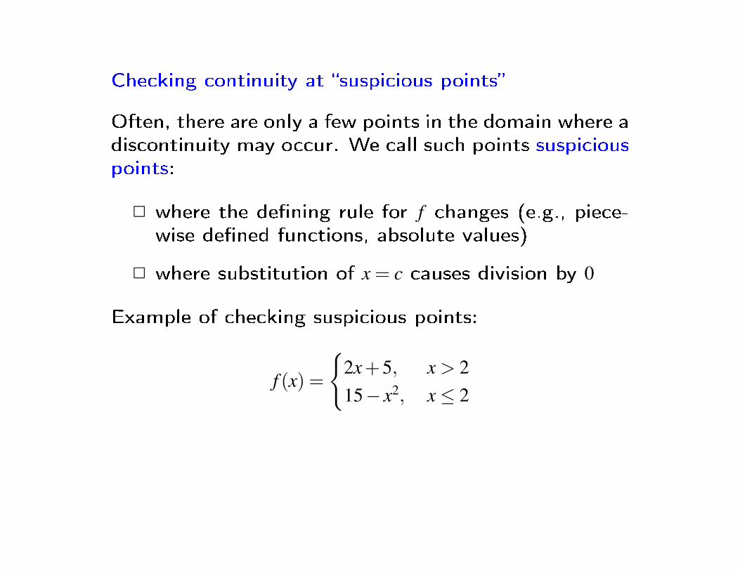
Checking continuity at �suspicious points�

Often, there are only a few points in the domain where adiscontinuity may occur. We call such points suspiciouspoints:

2 where the de�ning rule for f changes (e.g., piece-wise de�ned functions, absolute values)

2 where substitution of x = c causes division by 0

Example of checking suspicious points:

f (x) =

{2x+5, x > 215− x2, x≤ 2

Intermediate Value Theorem

Theorem. (Intermediate Value Theorem) If f is a con-tinuous function on the closed interval [a,b] and L issome number strictly between f (a) and f (b), then thereexists at least one number c on the open interval (a,b)such that f (c) = L.

In other words: if f is a continuous function on [a,b]then f (x) must take on all values between f (a) and f (b).

Important special case of the Intermediate Value The-orem:

Theorem. (Root location theorem) If f is continuouson the closed interval [a,b] and if f (a) and f (b) haveopposite algebraic signs, then f (c) = 0 for at least onenumber c on the open interval (a,b).

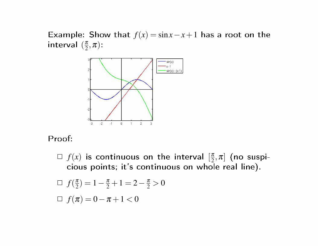
Example: Show that f (x) = sinx−x+1 has a root on theinterval (π

2 ,π):

Proof:

2 f (x) is continuous on the interval [π2 ,π] (no suspi-cious points; it's continuous on whole real line).

2 f (π

2) = 1− π

2 +1 = 2− π

2 > 0

2 f (π) = 0−π +1 < 0

2 (i.e., L = 0 is strictly between f (π

2) and f (π))

2 Therefore f (x) has at least one root in (π

2 ,π) byRoot location theorem (or by Intermediate ValueTheorem)

Exponentials and Logarithms (SBS 2.4)

Recall that we can already de�ne bx for any rationalnumber x:

2 For natural (counting) numbers n, we have bn =b ·b ·b · · · · ·b (n factors).

2 If b 6= 0, then b0 = 1, and b−n = 1bn.

2 If b > 0, then b1/n = n√

b.

2 If m, n are integers and m/n is a reduced fraction,then bm/n = (b1/n)m = n

√bm.

These steps work us up from counting numbers to anyrational number m

n .

We now want to extend the idea to all real numbers.

Completeness of the reals

For any real number x there is a sequence rn of rationalnumbers such that

x = limx→∞

rn.

That is, for any ε > 0 there is a number N such thatn > N ⇒ |x− rn|< ε.

As n gets bigger and bigger, rn gets closer and closerto the real number x.

This means that we can approximate any real numberto any degree of accuracy by a rational number.

Exponential functions

De�nition. Let x be a real number and let rn be a se-quence of rational numbers such that x = limx→∞ rn.Then the exponential function with base b, b> 0 (b 6= 1),is given by

bx = limn→∞

brn

b is called the base and x is the exponent.

[Do not confuse these with power functions f (x) = xp.Here the variable is in the exponent. In a power func-tion, it is in the base.]

Properties of the exponential function

Let x and y be any real numbers, and let a and b bepositive real numbers.

Equality rule: If b 6= 1, then bx = by i� x = y

Inequality rules: If x > y and b > 1, then bx > by

If x > y and 0 < b < 1, then bx < by

Product rule: bxby = bx+y

Quotient rule: bx

by = bx−y

Power rules: (bx)y = bxy; (ab)x = axbx; (ab)

x = ax

bx

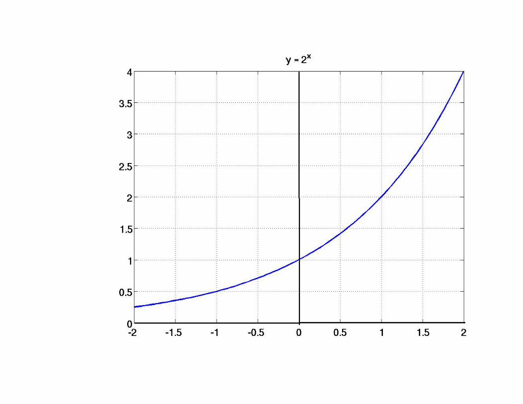
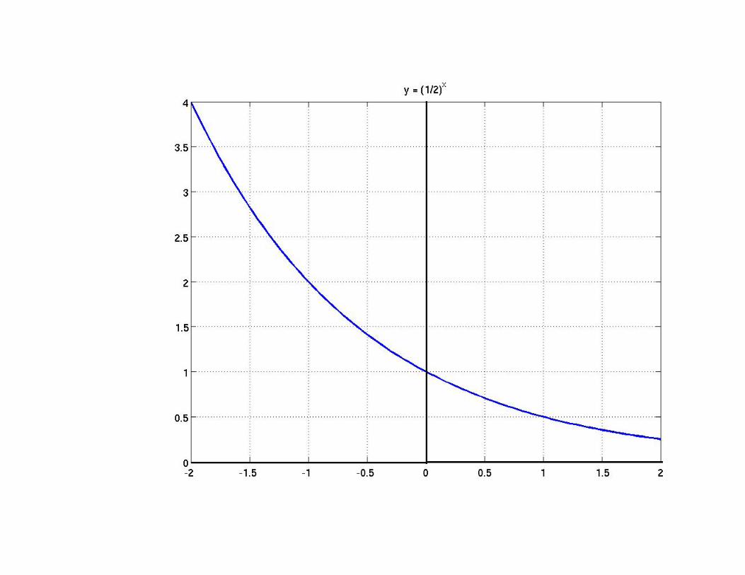
Graphical properties:

2 The exponential function f (x) = bx is continuous forall real numbers x.

2 bx > 0

2 The graph is always rising for b > 1 and alwaysfalling for 0 < b < 1.

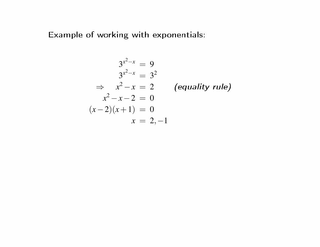
Example of working with exponentials:

3x2−x = 93x2−x = 32

⇒ x2− x = 2 (equality rule)

x2− x−2 = 0(x−2)(x+1) = 0

x = 2,−1

Logarithmic functions

y = bx (b > 0, b 6= 1) is monotonic, so the exponential hasan inverse.

If b > 0 and b 6= 1, the logarithm of x to the base b is thefunction y = logb x that satis�es by = x.

y = logbx means by = x

Note that since by = x, this means that we can only takethe logarithm of positive numbers.

I.e., the domain of the logarithm (which is the rangeof the exponential) is (0,∞).

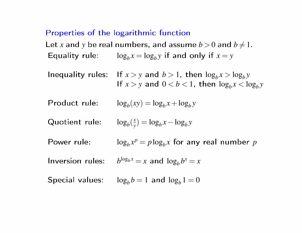
Properties of the logarithmic function

Let x and y be real numbers, and assume b> 0 and b 6= 1.Equality rule: logb x = logb y if and only if x = y

Inequality rules: If x > y and b > 1, then logb x > logb yIf x > y and 0 < b < 1, then logb x < logb y

Product rule: logb(xy) = logb x+ logb y

Quotient rule: logb(xy) = logb x− logb y

Power rule: logb xp = p logb x for any real number p

Inversion rules: blogb x = x and logb bx = x

Special values: logb b = 1 and logb 1 = 0

y = log2(x)

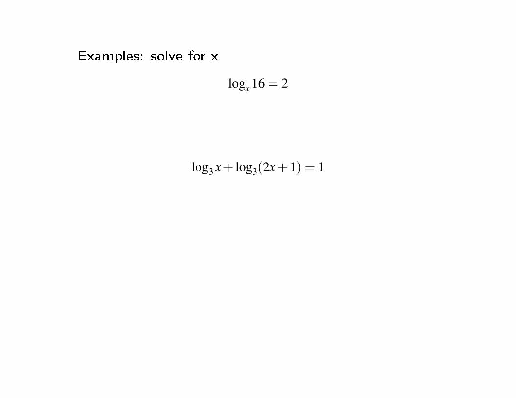
Examples: solve for x

logx 16 = 2

log3 x+ log3(2x+1) = 1

Natural exponential and natural logarithm

e = limn→∞

(1+

1n

)n

e≈ 2.7182818 · · ·

2 Notation: exp(x) = ex is the natural exponential

2 Natural Logarithm is the log base e, loge x, and isoften written lnx

2 Common Logarithm is the log base 10, log10 x, andis written logx

2 Beware: the notation � logx� is often used to rep-resent whichever base is the standard base in aparticular �eld (or a particular course).

2 But � lnx� always means the Natural Logarithm.

2 In this class, logx or log10 x will always mean thecommon logarithm and lnx or loge x will mean thenatural logarithm. For any other base we writelogb x.

Basic properties of the natural logarithm:(logarithm base e)

2 ln1 = 0

2 lne = loge e = 1

2 elnx = x for all x > 0

2 lney = y for all y

2 by = ey lnb for any b > 0 (b 6= 1)

Theorem. (Change of base theorem)

logb x =lnxlnb

for any b > 0 (b 6= 1).

Important, for example, for taking logarithms on a cal-culator or in many software packages, which often onlydo common and natural logarithms.

Example: Find N such that eN = 102x:

Example: an object moves along a straight line suchthat after t seconds, its velocity is given by

v(t) = 10log5 t +3log2 t

in ft/sec. How long will it take for the velocity to reach20 ft/sec?

What is so natural about the natural log?

Many important growth (and decay) processes are de-scribed in terms of natural exponentials and logarithms.For example,

2 Can be used to describe some types of biologicalcolony growthe.g., exponential growth of E. Coli bacteria

2 Describes continuous compound interest (see ex-amples in 2.4)

2 Newton's law of cooling (see problem 69 in 2.4)

2 Many other applications such as disease propaga-tion, radioactive decay...

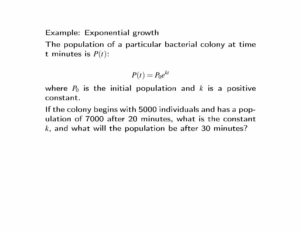
Example: Exponential growth

The population of a particular bacterial colony at timet minutes is P(t):

P(t) = P0ekt

where P0 is the initial population and k is a positiveconstant.

If the colony begins with 5000 individuals and has a pop-ulation of 7000 after 20 minutes, what is the constantk, and what will the population be after 30 minutes?

Example: continuous compounding interest

If D dollars are compounded n times per year at anannual interest rate r, then the Future Value after tyears is

A(t) = D(

1+rn

)nt

If the compounding interest is continuous, the FutureValue is

A(t) = Dert