119
Scalable Uncertainty Management 05 – Query Evaluation in Probabilistic Databases Rainer Gemulla Jun 1, 2012

Scalable Uncertainty Management05 – Query Evaluation in Probabilistic Databases
Rainer Gemulla
Jun 1, 2012

Overview
In this lecture
Primer: relational calculus
Understand complexity of query evaluation
How to determine whether a query is “easy” or “hard”
How to efficently evaluate easy queries→ extensional query evaluation
How to evaluate hard queries→ intensional query evaluation
How to approximately evaluate queries
Not in this lecture
Possible answer set semantics
Most representation systems but tuple-independent databases
2 / 119

Outline
1 Primer: Relational Calculus
2 The Query Evaluation Problem
3 Extensional Query EvaluationSyntactic IndependenceSix Simple RulesTractability and CompletenessExtensional Plans
4 Intensional Query EvaluationSyntactic independence5 Simple RulesQuery CompilationApproximation Techniques
5 Summary
3 / 119
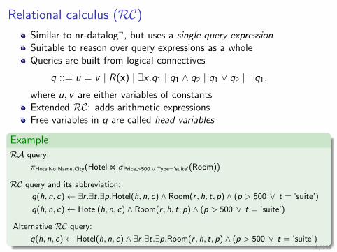
Relational calculus (RC)
Similar to nr-datalog¬, but uses a single query expressionSuitable to reason over query expressions as a wholeQueries are built from logical connectives
q ::= u = v | R(x) | ∃x .q1 | q1 ∧ q2 | q1 ∨ q2 | ¬q1,
where u, v are either variables of constantsExtended RC: adds arithmetic expressionsFree variables in q are called head variables
ExampleRA query:
πHotelNo,Name,City(Hotel on σPrice>500∨Type=’suite’(Room))
RC query and its abbreviation:
q(h, n, c)← ∃r .∃t.∃p.Hotel(h, n, c) ∧ Room(r , h, t, p) ∧ (p > 500 ∨ t = ’suite’)
q(h, n, c)← Hotel(h, n, c) ∧ Room(r , h, t, p) ∧ (p > 500 ∨ t = ’suite’)
Alternative RC query:
q(h, n, c)← Hotel(h, n, c) ∧ ∃r .∃t.∃p.Room(r , h, t, p) ∧ (p > 500 ∨ t = ’suite’)4 / 119

Boolean query
Definition
A Boolean query is an RC query with no head variables.
Asks whether the query result is emptyCan be obtained from RC-query by
1 Adding existential quantifiers for the head variables2 Replacing head variables by constants (potential results)
ExampleRC-query:
q(h, n, c)← Hotel(h, n, c) ∧ ∃r .∃t.∃p.Room(r , h, t, p) ∧ (p > 500 ∨ t = ’suite’)
Boolean RC-query (“Is there an answer?”):
q ← ∃h.∃n.∃c.Hotel(h, n, c) ∧ ∃r .∃t.∃p.Room(r , h, t, p) ∧ (p > 500 ∨ t = ’suite’)
Another Boolean RC-query (“Is (H1,Hilton,Paris) an answer?”):
q ← Hotel(’H1’, ’Hilton’, ’Paris’)∧∃r .∃t.∃p.Room(r , ’H1’, t, p)∧ (p > 500 ∨ t = ’suite’)
5 / 119
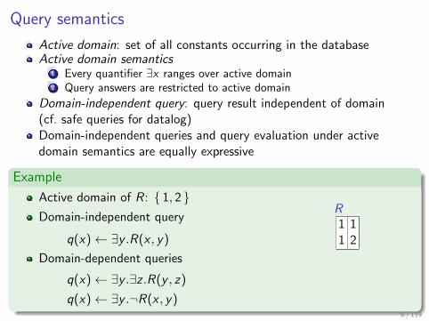
Query semantics
Active domain: set of all constants occurring in the databaseActive domain semantics
1 Every quantifier ∃x ranges over active domain2 Query answers are restricted to active domain
Domain-independent query: query result independent of domain(cf. safe queries for datalog)Domain-independent queries and query evaluation under activedomain semantics are equally expressive
Example
Active domain of R: { 1, 2 }Domain-independent query
q(x)← ∃y .R(x , y)
Domain-dependent queries
q(x)← ∃y .∃z .R(y , z)
q(x)← ∃y .¬R(x , y)6 / 119
R1 11 2

Relationships between query languages
Theorem
Each row of languages in the following table is equally expressive (weconsider only safe rules with a single output relation for nr-datalog¬ anddomain-independent rules for RC).
Relational algebra nr-datalog¬ Relational calculus
SPJR No repeated head ∃, ∧predicates, no negation (conjunctive queries: CQ)
SPJRU No negation ∃, ∧, ∨(positive RA) (nr-datalog) (unions of CQ: UCQ)
SPJRUD – ∃,∧,∨,¬(RA) (nr-datalog¬) (RC)
7 / 119

Outline
1 Primer: Relational Calculus
2 The Query Evaluation Problem
3 Extensional Query EvaluationSyntactic IndependenceSix Simple RulesTractability and CompletenessExtensional Plans
4 Intensional Query EvaluationSyntactic independence5 Simple RulesQuery CompilationApproximation Techniques
5 Summary
8 / 119

The query evaluation problem
Database systems are expected to scale to large datasets andparallelize to a large number of processors→ Same behavior is expected from probabilistic databases
We consider the possible tuple semantics, i.e., a query answer is anordered set of answer-probability pairs
{ (t1, p1), (t2, p2), . . . } with p1 ≥ p2 ≥ . . .
Definition (Query evaluation problem)
Fix a query q. Given a (representation of a) probabilistic database D and apossible answer tuple t, compute its marginal probability P ( t ∈ q(D) ).
9 / 119
Questions of interest
Characterize which queries are hard→ Understand what makes query evaluation hard
Given a query, determine whether it is hard→ Guide query processing
Given an easy query, solve the QEP→ Be efficient whenever possible
Given a hard query, solve the QEP (exactly or approximately)→ Don’t give up on hard queries
10 / 119

Query evaluation on deterministic databases
Definition
The data complexity of a query q is the complexity of evaluating it as afunction of the size of the input database. A query is tractable if its datacomplexity is in polynomial time; otherwise, it is intractable.
Example
Fix a relation schema R and consider an instance I with n tuples
q(R) = R → O(n)
q(R) = σE (R)→ O(n)
q(R) = πU(R)→ O(n2); can be tightened
Theorem
On deterministic databases, the data complexity of every RA query is inpolynomial time. Thus query evaluation is always tractable.
11 / 119

Query evaluation on probabilistic databases
Corollary
Query evaluation over probabilistic databases is tractable.
Proof.
Fix query q. Given a probabilistic database D = (I,P) withI =
{I 1, . . . , I n
}, perform the following steps:
1 Compute q(I k) for 1 ≤ k ≤ n → polynomial time
2 For each tuple t ∈ q(I k) for some k, compute
P ( t ∈ q(D) ) =∑
k:t∈q(I k )
P( I k )
→ polynomially many tuples, polynomial time per tuple
This result is treacherous: It talks about probabilisticdatabases but not about probabilistic representation systems!
12 / 119

Lineage trees and the query evaluation problem
Example
q(h)← ∃n.∃c.Hotel(h, n, c) ∧ ∃r .∃t.∃p.Room(r , h, t, p) ∧ (p > 500 ∨ t = ’suite’)
Room (R)
RoomNo Type HotelNo PriceR1 Suite H1 $50 X1
R2 Single H1 $600 X2
R3 Double H1 $80 X3
Hotel (H)
HotelNo Name CityH1 Hilton SB X4
ExpensiveHotels
HotelNoH1 X4 ∧ (X1 ∨ X2)
Theorem
Fix a RA query q. Given a boolean pc-table (T ,P), we can compute thelineage Φt of each possible output tuple t in polynomial time, where Φt isa propositional formula. We have
P ( t ∈ q(T ) ) = P ( Φt ) .
13 / 119

How can we compute Φt?
A naive approach
Let ω(Φ) be the set of assignments over Var(T ) that make Φ true. Thenapply P ( Φ ) =
∑θ∈ω(Φ) P ( θ ).
Exponential time: n variables → 2n assignments to check!
Definition (Model counting problem)
Given a propositional formula Φ, count the number of satisfyingassignments #Φ = |ω(Φ)|.
Definition (Probability computation problem)
Given a propositional formula Φ and a probability P ( X ) ∈ [0, 1] for eachvariable X , compute the probability P ( Φ ) =
∑θ∈ω(Φ) P ( θ ).
14 / 119

Model counting is a special case of probability computation
Suppose we have an algorithm to compute P ( Φ )
We can use the algorithm to compute #Φ
Define P ( X ) = 12 for every variable X
P ( θ ) = 1/2n for every assignment (n = number of variables)
#Φ = P ( Φ ) · 2n
Example
Φ = (X1 ∨ X2) ∧ X4; n = 3
#Φ = 3
P ( Φ ) = 38 = #Φ
2n
X1 X2 X4 Φθ P ( θ )0 0 0 FALSE 1/80 0 1 FALSE 1/80 1 0 FALSE 1/80 1 1 TRUE 1/81 0 0 FALSE 1/81 0 1 TRUE 1/81 1 0 FALSE 1/81 1 1 TRUE 1/8
15 / 119

The complexity class #P
Definition
The complexity class #P consists of all function problems of the followingtype: Given a polynomial-time, non-deterministic Turing machine,compute the number of accepting computations.
Theorem (Valiant, 1979)
Model counting (#SAT) is complete for #P.
NP asks whether there exists at least one accepting computation
#P counts the number of accepting computations
SAT is NP-complete
#SAT is #P-complete
Directly implies that probability computation is hard for #P!
16 / 119

A graph problem
Definition (Bipartite vertex cover)
Given a bipartite graph (V ,E), compute |{S ⊆ V : (u,w) ∈ E → u ∈ S ∨ w ∈ S }|.
Example
X1
X2 Y1
X3 Y2
X4 Y3
X5
80 possible ways
Theorem (Provan and Ball, 1983)
Bipartite vertex cover is #P-complete.
17 / 119
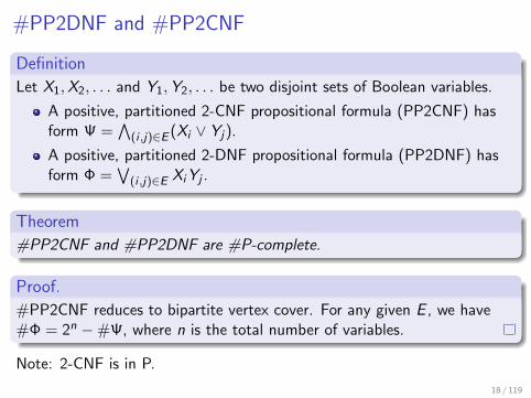
#PP2DNF and #PP2CNF
Definition
Let X1,X2, . . . and Y1,Y2, . . . be two disjoint sets of Boolean variables.
A positive, partitioned 2-CNF propositional formula (PP2CNF) hasform Ψ =
∧(i ,j)∈E (Xi ∨ Yj).
A positive, partitioned 2-DNF propositional formula (PP2DNF) hasform Φ =
∨(i ,j)∈E XiYj .
Theorem
#PP2CNF and #PP2DNF are #P-complete.
Proof.
#PP2CNF reduces to bipartite vertex cover. For any given E , we have#Φ = 2n −#Ψ, where n is the total number of variables.
Note: 2-CNF is in P.
18 / 119

A hard query
Theorem
The query evaluation problem of the CQ query H0 given by
H0 ← R(x) ∧ S(x , y) ∧ T (y)
on tuple-independent databases is hard for #P.
Proof.
Given a PP2DNF formula Φ =∨
(i ,j)∈E XiYj , whereE = { (Xe1 ,Ye1), (Xe2 ,Ye2), . . . }, construct the tuple-independent DB:
RXX1 1/2X2 1/2...
SX Y
Xe1 Ye1 1Xe2 Ye2 1
......
...
TYY1 1/2Y2 1/2...
Then #Φ = 2n P ( H0 ), where n is the total number of variables.19 / 119

More hard queries
Theorem
All of the following RC queries on tuple-independent databases are#P-hard:
H0 ← R(x) ∧ S(x , y) ∧ T (y)
H1 ← [R(x0) ∧ S(x0, y0)] ∨ [S(x1, y1) ∧ T (y1)]
H2 ← [R(x0) ∧ S1(x0, y0)] ∨ [S1(x1, y1) ∧ S2(x1, y1)]
∨ [S2(x2, y2) ∧ T (y2)]
...
Queries can be tractable even if they have intractable subqueries!q(x , y)← R(x) ∧ S(x , y) ∧ T (y) is tractable
q ← H0 ∨ T (y) is tractable
20 / 119

Extensional and intensional query evaluation
We’ll say more about data complexity as we go
Extensional query evaluationI Evaluation process guided by query expression qI Not always possibleI When possible, data complexity is in polynomial time
Extensional plansI Extensional query evaluation in the databaseI Only minor modifications to RDBMS necessaryI Scalability, parallelizability retained
Intensional query evaluationI Evaluation process guided by query lineageI Reduces query evaluation to the problem of computing the probability
of a propositional formulaI Works for every query
21 / 119

Outline
1 Primer: Relational Calculus
2 The Query Evaluation Problem
3 Extensional Query EvaluationSyntactic IndependenceSix Simple RulesTractability and CompletenessExtensional Plans
4 Intensional Query EvaluationSyntactic independence5 Simple RulesQuery CompilationApproximation Techniques
5 Summary
22 / 119

Problem statement
Tuple-independent databaseI Each tuple t annotated with a unique boolean variable Xt
I We write P ( t ) = P ( Xt )Boolean query Q
I With lineage ΦQ
I We write P ( Q ) = P ( ΦQ )Goal: compute P ( Q ) when Q is tractable
I Evaluation process guided by query expression qI I.e., without first computing lineage!
Example
BirdsSpecies PFinch 0.80 X1
Toucan 0.71 X2
Nightingale 0.65 X3
Humming bird 0.55 X4
P ( Finch ) = P ( X1 ) = 0.8
Is there a finch? Q ← Birds(Finch)I ΦQ = X1
I P ( Q ) = 0.8
Is there some bird? Q ← Birds(s)?I ΦQ = X1 ∨ X2 ∨ X3 ∨ X4
I P ( Q ) ≈ 99.1%23 / 119

Overview of extensional query evaluation
Break the query into “simpler” subqueries
By applying one of the rules1 Independent-join2 Independent-union3 Independent-project4 Negation5 Inclusion-exclusion (or Mobius inversion formula)6 Attribute ranking
Each rule application is polynomial in size of database
Main results for UCQ queriesI Completeness: Rules succeed iff query is tractableI Dichotomy: Query is #P-hard if rules don’t succeed
24 / 119
Outline
1 Primer: Relational Calculus
2 The Query Evaluation Problem
3 Extensional Query EvaluationSyntactic IndependenceSix Simple RulesTractability and CompletenessExtensional Plans
4 Intensional Query EvaluationSyntactic independence5 Simple RulesQuery CompilationApproximation Techniques
5 Summary
25 / 119

Unifiable atoms
Definition
Two relational atoms L1 and L2 are said to be unifiable (or to unify) ifthey have a common image. I.e., there exists substitutions such thatL1[a1/x1] = L2[a2/x2], where x1 are the variables in L1 and x2 are thevariables in L2.
ExampleUnifiable:
R(a), R(a) via [], []
R(x), R(y) via [a/x ], [a/y ]
R(a, y), R(x , y) via [b/y ], [(a, b)/(x , y)]
R(a, b), R(x , y) via [], [(a, b)/(x , y)]
R(a, y), R(x , b) via [b/y ], [a/x ]
Not unifiable:
R(a), R(b)
R(a, y), R(b, y)
R(x), S(x)
Unifiable atoms must use the same relation symbol.
26 / 119
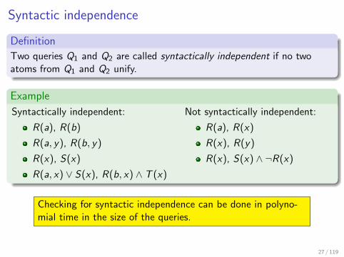
Syntactic independence
Definition
Two queries Q1 and Q2 are called syntactically independent if no twoatoms from Q1 and Q2 unify.
Example
Syntactically independent:
R(a), R(b)
R(a, y), R(b, y)
R(x), S(x)
R(a, x) ∨ S(x), R(b, x) ∧ T (x)
Not syntactically independent:
R(a), R(x)
R(x), R(y)
R(x), S(x) ∧ ¬R(x)
Checking for syntactic independence can be done in polyno-mial time in the size of the queries.
27 / 119

Syntactic independence and probabilistic independence
Proposition
Let Q1,Q2, . . . ,Qk be pairwise syntactically independent. ThenQ1, . . . ,Qk are independent probabilistic events.
Proof.
The sets Var(ΦQ1), . . . ,Var(ΦQk) are pairwise disjoint, i.e., the lineage
formulas do not share any variables. Since all variables are independent(because we have a tuple-independent database), the propositionfollows.
ExampleSyntactically independent:
R(a), R(b)
R(a, y), R(b, y)
R(x), S(x)
R(a, x) ∨ S(x), R(b, x) ∧ T (x)
Not syntactically independent:
R(a), R(x)
R(x), R(y)
R(x), S(x) ∧ ¬R(x)
28 / 119

Probabilistic independence and syntactic independence
Proposition
Probabilistic independence does not necessarily imply syntacticindependence.
Example
Consider
Q1 ← R(x , y) ∧ R(x , x)
Q2 ← R(a, b)
If ΦQ1 does not contain XR(a,b), Q1 and Q2 are independent
Otherwise, ΦQ1 contains XR(a,b) and therefore XR(a,b) ∧ XR(a,a)
Then, ΦQ1 also contains XR(a,a) ∧ XR(a,a) = XR(a,a)
Thus, by the absorption law,
(XR(a,b) ∧ XR(a,a)) ∨ XR(a,a) = XR(a,a)
XR(a,b) can be eliminated from ΦQ1 so that Q1 and Q2 are independent
29 / 119
Outline
1 Primer: Relational Calculus
2 The Query Evaluation Problem
3 Extensional Query EvaluationSyntactic IndependenceSix Simple RulesTractability and CompletenessExtensional Plans
4 Intensional Query EvaluationSyntactic independence5 Simple RulesQuery CompilationApproximation Techniques
5 Summary
30 / 119

Base case: Atoms
Definition
If Q is an atom, i.e., of form Q = R(a), simply lookup its probability inthe database.
Example
Sightings
Name Species PMary Finch 0.8 X1
Mary Toucan 0.3 X2
Susan Finch 0.2 X3
Susan Toucan 0.5 X4
Susan Nightingale 0.6 X5
Did Mary see a toucan?
Q = Sightings(Mary,Toucan)
P ( Q ) = 0.3
31 / 119

Rule 1: Independent-join
Definition
If Q1 and Q2 are syntactically independent, then
P ( Q1 ∧ Q2 ) = P ( Q1 ) · P ( Q2 ) . (independent-join)
Example
Sightings
Name Species PMary Finch 0.8 X1
Mary Toucan 0.3 X2
Susan Finch 0.2 X3
Susan Toucan 0.5 X4
Susan Nightingale 0.6 X5
Did both Mary and Susan see a toucan?
Q = S(Mary,Toucan) ∧ S(Susan,Toucan)
Q1 = S(Mary,Toucan) P ( Q1 ) = 0.3
Q2 = S(Susan,Toucan) P ( Q2 ) = 0.5
P ( Q ) = P ( Q1 ) · P ( Q2 ) = 0.15
32 / 119

Rule 2: Independent-union
Definition
If Q1 and Q2 are syntactically independent, then
P ( Q1 ∨ Q2 ) = 1− (1− P ( Q1 ))(1− P ( Q2 )). (independent-union)
Example
Sightings
Name Species PMary Finch 0.8 X1
Mary Toucan 0.3 X2
Susan Finch 0.2 X3
Susan Toucan 0.5 X4
Susan Nightingale 0.6 X5
Did Mary or Susan see a toucan?
Q = S(Mary,Toucan) ∨ S(Susan,Toucan)
Q1 = S(Mary,Toucan) P ( Q1 ) = 0.3
Q2 = S(Susan,Toucan) P ( Q2 ) = 0.5
P ( Q ) =1− (1− P ( Q1 ))(1− P ( Q2 )) = 0.65
33 / 119

Root variables and separator variables
Definition
Consider atom L and query Q. Denote by Pos(L, x) the set of positionswhere x occurs in Q (maybe empty). If Q is of form Q = ∃x .Q ′:
Variable x is a root variable if it occurs in all atoms, i.e.,Pos(L, x) 6= ∅ for every atom L that occurs in Q ′.
A root variable x is a separator variable if for any two atoms thatunify, x occurs on a common position, i.e.,Pos(L1, x) ∩ Pos(L2, x) 6= ∅.
Example
Q1 ← ∃x .Likes(a, x) ∧ Likes(x , a)
Pos(Likes(a, x), x) = { 2 }Pos(Likes(x , a), x) = { 1 }x is root variable
x is no separator variable
Q2 ← ∃x .Likes(a, x) ∧ Likes(x , x)
x is root variable
x is a separator variable
Q3 ← ∃x .Likes(a, x) ∧ Popular(a)
x is no root variable
x is no separator variable 34 / 119
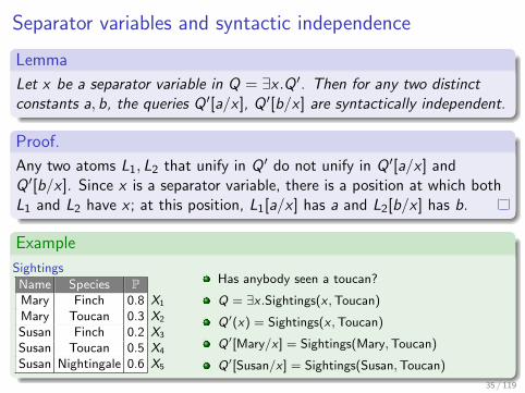
Separator variables and syntactic independence
Lemma
Let x be a separator variable in Q = ∃x .Q ′. Then for any two distinctconstants a, b, the queries Q ′[a/x ], Q ′[b/x ] are syntactically independent.
Proof.
Any two atoms L1, L2 that unify in Q ′ do not unify in Q ′[a/x ] andQ ′[b/x ]. Since x is a separator variable, there is a position at which bothL1 and L2 have x ; at this position, L1[a/x ] has a and L2[b/x ] has b.
Example
Sightings
Name Species PMary Finch 0.8 X1
Mary Toucan 0.3 X2
Susan Finch 0.2 X3
Susan Toucan 0.5 X4
Susan Nightingale 0.6 X5
Has anybody seen a toucan?
Q = ∃x .Sightings(x ,Toucan)
Q ′(x) = Sightings(x ,Toucan)
Q ′[Mary/x ] = Sightings(Mary,Toucan)
Q ′[Susan/x ] = Sightings(Susan,Toucan)
35 / 119

Rule 3: Independent-project
Definition
If Q is of form Q = ∃x .Q ′ and x is a separator variable, then
P ( Q ) = 1−∏
a∈ADom
(1− P
(Q ′[a/x ]
)), (independent-project)
where ADom is the active domain of the database.
Example
Sightings
Name Species PMary Finch 0.8 X1
Mary Toucan 0.3 X2
Susan Finch 0.2 X3
Susan Toucan 0.5 X4
Susan Nightingale 0.6 X5
Has anybody seen a toucan?
Q = ∃x .S(x ,Toucan)
Q ′ = S(x ,Toucan)
P ( Q ) = 1−∏
x∈{M,S,F,... }
(1− P ( S(x ,T) ))
= 1− (1− 0.3)(1− 0.5)1 · · · 1= 0.65
36 / 119

Rule 4: Negation
Definition
If the query is ¬Q, then
P (¬Q ) = 1− P ( Q ) (negation)
Example
Sightings
Name Species PMary Finch 0.8 X1
Mary Toucan 0.3 X2
Susan Finch 0.2 X3
Susan Toucan 0.5 X4
Susan Nightingale 0.6 X5
Did nobody see a toucan?
Q = ¬[∃x .S(x ,Toucan)]
P ( Q ) = 1− P (∃x .S(x ,Toucan) ) = 0.35
37 / 119

Rule 5: Inclusion-exclusion
Definition
Suppose Q = Q1 ∧ Q2 ∧ . . .Qk . Then,
P ( Q ) = −∑
∅6=S⊆{ 1,...,k }
(−1)|S| P( ∨i∈S
Qi
)(inclusion-exclusion)
Example
Q1
Q2 Q3
123
1
23
12 13
2 3
1 2 3 12 13 23 123 P ( Q1 ∧ Q2 ∧ Q3 ) =1 0 0 1 1 0 1 +P ( Q1 )1 1 0 2 1 1 2 +P ( Q2 )1 1 1 2 2 2 3 +P ( Q3 )0 0 1 1 1 1 2 −P ( Q1 ∨ Q2 )-1 0 0 0 0 0 1 −P ( Q1 ∨ Q3 )-1 -1 -1 -1 -1 -1 0 −P ( Q2 ∨ Q3 )0 0 0 0 0 0 1 +P ( Q1 ∨ Q2 ∨ Q3 )
38 / 119

Inclusion-exclusion for independent-projectGoal of inclusion-exclusion is to apply the rewrite
(∃x1.Q1)∨ (∃x2.Q2) ≡ ∃x .(Q1[x/x1]∨Q2[x/x2]).
Example
Sightings
Name Species PMary Finch 0.8Mary Toucan 0.3Susan Finch 0.2Susan Toucan 0.5Susan Nightingale 0.6
Has both Mary seen some bird and someone seen a finch?
P ( (∃x .S(M, x)) ∧ (∃y .S(y ,F)) ) (ie)
= P (∃x .S(M, x) ) + P (∃y .S(y ,F) )− P ( (∃x .S(M, x)) ∨ (∃y .S(y ,F)) ) (ip/ip/rewrite)
= 0.86 + 0.84− P ( ∃x .S(M, x) ∨ S(x ,F) )
= 1.7− P ( ∃x .S(M, x) ∨ S(x ,F) )
Now we are stuck → Need another rule (attribute-constant ranking)!39 / 119

Rule 6: Attribute ranking
Definition
Attribute-constant ranking. If Q is a query that contains a relation nameR with attribute A, and there exists two unifiable atoms such that the firsthas constant a at position A and the second has a variable, substitute eachoccurence of form R(. . .) by R1(. . .) ∨ R2(. . .), where
R1 = σA=a(R), R2 = σA6=a(R).
Attribute-attribute ranking. If Q is a query that contains a relation nameR with attributes A and B, substitute each occurence of form R(. . .) byR1(. . .) ∨ R2(. . .) ∨ R3(. . .), where
R1 = σA<B(R), R2 = σA=B(R), R3 = σA>B(R).
Syntactic rewrites. For selections of form σA=·, decrease the arity of theresulting relation by 1 and add an equality predicate.
40 / 119
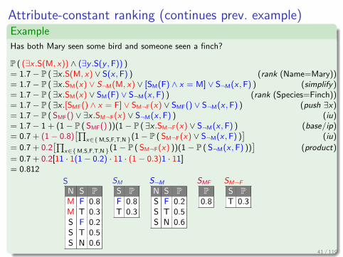
Attribute-constant ranking (continues prev. example)ExampleHas both Mary seen some bird and someone seen a finch?
P ( (∃x .S(M, x)) ∧ (∃y .S(y ,F)) )= 1.7− P ( ∃x .S(M, x) ∨ S(x ,F) ) (rank (Name=Mary))= 1.7− P ( ∃x .SM(x) ∨ S¬M(M, x) ∨ [SM(F) ∧ x = M] ∨ S¬M(x ,F) ) (simplify)= 1.7− P ( ∃x .SM(x) ∨ SM(F) ∨ S¬M(x ,F) ) (rank (Species=Finch))= 1.7− P ( ∃x .[SMF() ∧ x = F] ∨ SM¬F(x) ∨ SMF() ∨ S¬M(x ,F) ) (push ∃x)= 1.7− P ( SMF() ∨ ∃x .SM¬F(x) ∨ S¬M(x ,F) ) (iu)= 1.7− 1 + (1− P ( SMF() ))(1− P ( ∃x .SM¬F(x) ∨ S¬M(x ,F) ) (base/ip)= 0.7 + (1− 0.8)
[∏x∈{M,S,F,T,N }(1− P ( SM¬F(x) ∨ S¬M(x ,F) )
](iu)
= 0.7 + 0.2[∏
x∈{M,S,F,T,N }(1− P ( SM¬F(x) ))(1− P ( S¬M(x ,F) ))]
(product)
= 0.7 + 0.2[11 · 1(1− 0.2) · 11 · (1− 0.3)1 · 11]= 0.812
41 / 119
SN S PM F 0.8M T 0.3S F 0.2S T 0.5S N 0.6
SM
S PF 0.8T 0.3
S¬MN S PS F 0.2S T 0.5S N 0.6
SMF
P0.8
SM¬FS PT 0.3
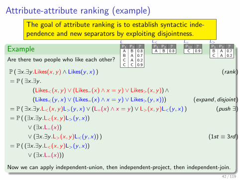
Attribute-attribute ranking (example)
The goal of attribute ranking is to establish syntactic inde-pendence and new separators by exploiting disjointness.
ExampleAre there two people who like each other?
P ( ∃x .∃y .Likes(x , y) ∧ Likes(y , x) ) (rank)
= P (∃x .∃y .(Likes<(x , y) ∨ (Likes=(x) ∧ x = y) ∨ Likes>(x , y))∧(Likes<(y , x) ∨ (Likes=(x) ∧ x = y) ∨ Likes>(y , x))) (expand , disjoint)
= P (∃x .∃y .L<(x , y)L>(y , x) ∨ (L=(x) ∧ x = y) ∨ L>(x , y)L<(y , x) ) (push ∃)
= P ( (∃x .∃y .L<(x , y)L>(y , x))
∨ (∃x .L=(x))
∨ (∃x .∃y .L>(x , y)L<(y , x)) ) (1st ≡ 3rd)
= P ( (∃x .∃y .L<(x , y)L>(y , x))
∨ (∃x .L=(x)))
Now we can apply independent-union, then independent-project, then independent-join.
42 / 119
LP1 P2 PA B 0.8B A 0.7C A 0.2C C 0.9
L<P1 P2 PA B 0.8
L=P12 PC 0.9
L>P1 P2 PB A 0.7C A 0.2
Outline
1 Primer: Relational Calculus
2 The Query Evaluation Problem
3 Extensional Query EvaluationSyntactic IndependenceSix Simple RulesTractability and CompletenessExtensional Plans
4 Intensional Query EvaluationSyntactic independence5 Simple RulesQuery CompilationApproximation Techniques
5 Summary
43 / 119
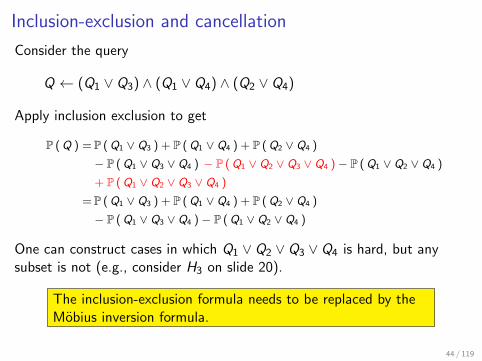
Inclusion-exclusion and cancellation
Consider the query
Q ← (Q1 ∨ Q3) ∧ (Q1 ∨ Q4) ∧ (Q2 ∨ Q4)
Apply inclusion exclusion to get
P (Q ) =P (Q1 ∨ Q3 ) + P (Q1 ∨ Q4 ) + P (Q2 ∨ Q4 )
− P (Q1 ∨ Q3 ∨ Q4 ) − P (Q1 ∨ Q2 ∨ Q3 ∨ Q4 )− P (Q1 ∨ Q2 ∨ Q4 )
+ P (Q1 ∨ Q2 ∨ Q3 ∨ Q4 )
=P (Q1 ∨ Q3 ) + P (Q1 ∨ Q4 ) + P (Q2 ∨ Q4 )
− P (Q1 ∨ Q3 ∨ Q4 )− P (Q1 ∨ Q2 ∨ Q4 )
One can construct cases in which Q1 ∨ Q2 ∨ Q3 ∨ Q4 is hard, but anysubset is not (e.g., consider H3 on slide 20).
The inclusion-exclusion formula needs to be replaced by theMobius inversion formula.
44 / 119
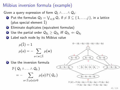
Mobius inversion formula (example)
Given a query expression of form Q1 ∧ . . . ∧ Qk :1 Put the formulas QS =
∨i∈S Qi , ∅ 6= S ⊆ { 1, . . . , j }, in a lattice
(plus special element 1)2 Eliminate duplicates (equivalent formulas)3 Use the partial order QS1 ≥ QS2 iff QS1 ⇐ QS2
4 Label each node by its Mobius value
µ(1) = 1
µ(u) = −∑
u<w≤1
µ(w)
5 Use the inversion formula
P ( Q1 ∧ . . . ∧ Qk )
= −∑
u<1:µ(u)6=0
µ(u)P ( Qu )
45 / 119
1
Q1 ∨ Q4Q1 ∨ Q3 Q2 ∨ Q4
Q1 ∨ Q2 ∨ Q3 ∨ Q4Q1 ∨ Q3 ∨ Q4 Q1 ∨ Q2 ∨ Q4
Q1 ∨ Q2 ∨ Q3 ∨ Q4
1
-1
-1
-1
1 1
0
Q ← (Q1 ∨ Q3) ∧ (Q1 ∨ Q4) ∧ (Q2 ∨ Q4)
P ( Q ) =P ( Q1 ∨ Q3 ) + P ( Q1 ∨ Q4 ) + P ( Q2 ∨ Q4 )
− P ( Q1 ∨ Q3 ∨ Q4 )− P ( Q1 ∨ Q2 ∨ Q4 )

An nondeterministic algorithm
Consider the algorithm:
1 As long as possible, apply one of the rules R1–R6
2 If all formulas are atoms, SUCCESS
3 If there is a formula that is not an atom, FAILURE
Definition
A rule is R6-safe if the above algorithm succeeds.
Order of rule application does not affect SUCCESS
Algorithm is polynomial in size of databaseI Easy to see for independent-join, independent-union, negation, Mobius
inversion formula, attribute ranking → do not depend on databaseI Independent-project increases number of queries by a factor of |ADom|→ applied at most k times, where k is the maximum arity of a relation
46 / 119

How the rules fail
Example
Consider the hard query
H0 ← ∃x .∃y .R(x) ∧ S(x , y) ∧ T (y)
independent-join, independent-union, independent-project, negation,Mobius inversion formula all do not apply
But we could rank S :
H0 ← H01 ∨ H02 ∨ H03
H01 ← ∃x .∃y .R(x) ∧ S<(x , y) ∧ T (y)
H02 ← ∃x .R(x) ∧ S=(x) ∧ T (x)
H03 ← ∃x .∃y .R(x) ∧ S>(y , x) ∧ T (y)
Now we are stuck at H01 and H03
47 / 119
Dichotomy theorem for UCQSafety is a syntactic property
Tractability is a semantic property
What is their relationship?
Theorem (Dalvi and Suciu, 2010)
For any UCQ query Q, one of the following holds:
Q is R6-safe, or
the data complexity of Q is hard for #P.
No queries of “intermediate” difficulty
Can check for tractability in time polynomial in database size(can be done by assuming an active domain of size 1)
Query complexity is unknown (Mobius inversion formula)
For RC, completeness/dichotomy unknown
We can handle all safe UCQ queries!
48 / 119
Outline
1 Primer: Relational Calculus
2 The Query Evaluation Problem
3 Extensional Query EvaluationSyntactic IndependenceSix Simple RulesTractability and CompletenessExtensional Plans
4 Intensional Query EvaluationSyntactic independence5 Simple RulesQuery CompilationApproximation Techniques
5 Summary
49 / 119

Overview of extensional plans
Can we evaluate safe queries directly in an RDBMS?
Extensional query evaluationI Based on the query expressionI Uses rules to break query into simpler piecesI For UCQ, detects whether queries are tractable or intractable
Extensional operatorsI Extend relational operators by probability computationI Standard database algorithms can be used
Extensional plansI Can be safe (correct) or unsafe (incorrect)I For tractable UCQ queries, we can always produce a safe planI Plan construction based on R6 rulesI Can be written in SQL (though not “best” approach)I Enables scalable query processing on probabilistic databases
50 / 119
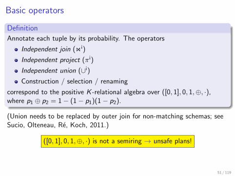
Basic operators
Definition
Annotate each tuple by its probability. The operators
Independent join (oni)
Independent project (πi)
Independent union (∪i)
Construction / selection / renaming
correspond to the positive K -relational algebra over ([0, 1], 0, 1,⊕, ·),where p1 ⊕ p2 = 1− (1− p1)(1− p2).
(Union needs to be replaced by outer join for non-matching schemas; seeSucio, Olteneau, Re, Koch, 2011.)
([0, 1], 0, 1,⊕, ·) is not a semiring → unsafe plans!
51 / 119

Example plans
Who incriminates someonewho has an alibi?
Q1(w)← ∃s.∃x .Incriminates(w , s) ∧ Alibi(s, x)
Q2(w)← ∃s.Incriminates(w , s) ∧ ∃x .Alibi(s, x)
πiw
onis
Incriminates(w , s) Alibi(s, x)
M 1− (1− p1q1)(1− p1q2)(1− p2q3)S p3q3
M P C p1q1
M P F p1q2
M J B p2q3
S J B p3q3
πiw
onis
Incriminates(w , s)
πis
Alibi(s, x)
M 1− [1− p1(1− (1− q1)(1− q2))][1− p2q3]S p3q3
M P p1(1− (1− q1)(1− q2))M J p2q3
S J p3q3
P 1− (1− q1)(1− q2)J q3
Plan 1 Plan 2Incorrect (unsafe) Correct (safe)
Not all plans are safe!52 / 119
IncriminatesWitness Suspect
Mary Paul p1
Mary John p2
Susan John p3
AlibiSuspect Claim
Paul Cinema q1
Paul Friend q2
John Bar q3

Weighted sum
How to deal with the Mobius inversion formula?
Definition
The weighted sum of relations R1, . . . ,Rk with parameters µ1, . . . , µk isgiven by:(
µ1,...,µk∑U
(R1, . . . ,Rk)
)[] = R1 on · · · on Rk(
µ1,...,µk∑U
(R1, . . . ,Rk)
)(t) = µ1(R1(t)) + · · ·µk(Rk(t))
Intuitively,
Computes the natural join
Sums up the weighted probabilities of joining tuples
53 / 119

Weighted sum (example)
Example
Consider relations/subqueries V1(A,B) and V2(A,C ) and the query:
Q(x , y , z)← V1(x , y) ∧ V2(x , z)
Suppose we apply the Mobius inversion formula to get:
Q1(x , y) = V1(x , y) with µ1 = 1
Q2(x , z) = V2(x , z) with µ2 = 1
Q3(x , y , z) = V1(x , y) ∨ V2(x , z) with µ3 = −1
We obtain:
1,1,−1∑{ A,B,C }
(Q1,Q2,Q3)[] = Q1 on Q2 on Q3 = V1 on V2
1,1,−1∑{ A,B,C }
(Q1,Q2,Q3) = { (t, pt1 + pt2 − pt3 ) : t[AB] = t1 ∈ Q1, t[AC ] = t2 ∈ Q2,t[ABC ] = t3 ∈ Q3 }
54 / 119
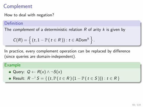
Complement
How to deal with negation?
Definition
The complement of a deterministic relation R of arity k is given by
C (R) ={
(t, 1− P ( t ∈ R )) : t ∈ ADomk}.
In practice, every complement operation can be replaced by difference(since queries are domain-independent).
Example
Query: Q ← R(x) ∧ ¬S(x)
Result: R −i S = { (t,P ( t ∈ R ) (1− P ( t ∈ S ))) : t ∈ R }
55 / 119

Computation of safe plans (1)
Definition
A query plan for Q is safe if it computes the correct probabilities for allinput databases.
Theorem
There is an algorithm A that takes in a query Q and outputs either FAILof a safe plan for Q. If Q is a UCQ query, A fails only if Q is intractable.
Key idea: Apply rules R1–R6, but produce a query plan instead ofcomputing probabilities
Extension to non-Boolean queries: treat head variables as “constants”
Ranking step produces “views” that are treated as base tables
56 / 119

Computation of safe plans (2)
1: if Q = Q1 ∧ Q2 and Q1,Q2 are syntactically independent then2: return plan(Q1) oni plan(Q2)3: end if4: if Q = Q1 ∨ Q2 and Q1,Q2 are syntactically independent then5: return plan(Q1) ∪i plan(Q2)6: end if7: if Q(x) = ∃z .Q1(x, z) and z is a separator variable then8: return πi
x(plan(Q1(x, z)))9: end if
10: if Q = Q1 ∧ . . . ∧ Qk , k ≥ 2 then11: Construct CNF lattice Q ′1, . . . ,Q
′m
12: Compute Mobius coefficients µ1, . . . , µm
13: return∑µ1,...,µm (plan(Q ′1), . . . , plan(Q ′m))
14: end if15: if Q = ¬Q1 then16: return C(planQ1)17: end if18: if Q(x) = R(x) where R is a base table (possibly ranked) then19: return R(x)20: end if21: otherwise FAIL
57 / 119

Computation of safe plans (example)
Q(w)← ∃s.∃x .Incriminates(w , s) ∧ Alibi(s, x)1 Apply independent-project to Q on s
I Q1(w , s)← ∃x .Incriminates(w , s) ∧ Alibi(s, x)
2 x is not a root variable in Q1 → push ∃x :Q2(w , s)← Incriminates(w , s) ∧ ∃x .Alibi(s, x)
3 Apply independent-join to Q2
I Q3(w , s)← Incriminates(w , s)I Q4(s)← ∃x .Alibi(s, x)
4 Q3 is an atom5 Apply independent-project to Q4 on x
I Q5(s, x) = Alibi(s, x)
6 Q5 is an atom
58 / 119
πiWitness
oniSuspect
Incriminates
πiSuspect
Alibi

Safe plans with PostgreSQL (example)
Q(w)← ∃s.∃x .Incriminates(w , s) ∧ Alibi(s, x)
Q4 ← πiSuspect(Alibi)
Q2 ← Incriminates oniSuspect Q4
Q ← πiWitness(Q2)
SELECT Witness , 1-PRODUCT(1-P) AS P
FROM (
SELECT Witness , Incriminates.Suspect ,
Incriminates.P * Q4.P as P
FROM Incriminates ,
(
SELECT Suspect , 1-PRODUCT(1-P) AS P
FROM Alibi
GROUP BY Suspect
) AS Q4
WHERE Incriminates.Suspect = Q4.Suspect
) AS Q2
GROUP BY Witness 59 / 119
πiWitness
oniSuspect
Incriminates
πiSuspect
Alibi

Deterministic tables
Often: Mix of probabilistic and deterministic tablesNaive approach: Assign probability 1 to tuples in a deterministic table→ Suboptimal: Some tractable queries are missed!
Example
If T is known to be deterministic, the query
Q ← R(x), S(x , y),T (y)
becomes tractable!
Why? S on T now is a tuple-independent table!
We can use the safe planπi∅[R(x) oni
x (S(x , y) ony T (y))]
Additional information about the nature of the tables (e.g.,deterministic, tuple-independent with keys, BID tables) canhelp extensional query processing.
60 / 119
Outline
1 Primer: Relational Calculus
2 The Query Evaluation Problem
3 Extensional Query EvaluationSyntactic IndependenceSix Simple RulesTractability and CompletenessExtensional Plans
4 Intensional Query EvaluationSyntactic independence5 Simple RulesQuery CompilationApproximation Techniques
5 Summary
61 / 119

Overview
Given a query Q(x), a TI database D; for each output tuple t
1 Compute the lineage Φ = ΦDQ(t)
I |Φ| = O(|ADom|m), where m is the number of variables in ΦI Data complexity is polynomial timeI Difference to extensional query evaluation: |Φ| depends on input→ rules exponential in |Φ| also exponential in the size of the input!
2 Compute the probability P( Φ )I Intensional query evaluation ≈ probability computation on
propositional formulasI Studied in verification and AI communitiesI Different approaches: rule-based evaluation, formula compilation,
approximation
Can deal with hard queries.
62 / 119
Example (tractable query)
Example
q(h)← ∃n.∃c.Hotel(h, n, c) ∧ ∃r .∃t.∃p.Room(r , h, t, p) ∧ (p > 500 ∨ t = ’suite’)
Room (R)
RoomNo Type HotelNo PriceR1 Suite H1 $50 X1
R2 Single H1 $600 X2
R3 Double H1 $80 X3
Hotel (H)
HotelNo Name CityH1 Hilton SB X4
ExpensiveHotels
HotelNoH1 X4 ∧ (X1 ∨ X2)
Φ = X4 ∧ (X1 ∨ X2)
P ( Φ ) = P (X4 ) [1− (1− P (X1 ))(1− P (X2 ))]
E.g., P (Xi ) = 12
for all i → P ( Φ ) = 0.375
ExpensiveHotels
HotelNo PH1 0.375
63 / 119

Example (intractable query)
Example
X1
X2 Y1
X3 Y2
X4
RX1 0.5X2 0.5X3 0.5X4 0.5
SX2 Y1 1X3 Y2 1
TY1 0.5Y2 0.5
H0 ← ∃x .∃y .R(x),S(x , y),T (y)
Φ = X2Y1 ∨ X3Y2
P ( Φ ) = 1− (1− P ( X2 )P ( Y1 ))(1− P ( X3 )P ( Y2 )) = 0.4375
Model counting: #Φ = 26 P ( Φ ) = 28
Bipartite vertex cover: #Ψ = 26 −#Φ = 36 = 2 · 3 · 3 · 2
64 / 119
Outline
1 Primer: Relational Calculus
2 The Query Evaluation Problem
3 Extensional Query EvaluationSyntactic IndependenceSix Simple RulesTractability and CompletenessExtensional Plans
4 Intensional Query EvaluationSyntactic independence5 Simple RulesQuery CompilationApproximation Techniques
5 Summary
65 / 119
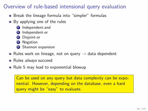
Overview of rule-based intensional query evaluation
Break the lineage formula into “simpler” formulas
By applying one of the rules1 Independent-and2 Independent-or3 Disjoint-or4 Negation5 Shannon expansion
Rules work on lineage, not on query → data dependent
Rules always succeed
Rule 5 may lead to exponential blowup
Can be used on any query but data complexity can be expo-nential. However, depending on the database, even a hardquery might be “easy” to evaluate.
66 / 119

Support
Definition
For a propositional formula Φ, denote by V (Φ) the set of variables thatoccur in Φ. Denote by Var(Φ) the set of variables on which Φ depends;Var(Φ) is called the support of Φ. X ∈ Var(Φ) iff there exists anassignment θ to all variables but X and constants a 6= b such thatΦ[θ ∪ {X 7→ a }] 6= Φ[θ ∪ {X 7→ b }].
Example
Φ = X ∨ (Y ∧ Z )
V (Φ) = {X ,Y ,Z }Var(Φ) = {X ,Y ,Z }
Φ = Y ∨ (X ∧ Y ) ≡ Y
V (Φ) = {X ,Y }Var(Φ) = {Y }
67 / 119

Syntactic independence
Definition
Φ1 and Φ2 are syntactically independent if they have disjoint support, i.e.,Var(Φ1) ∩ Var(Φ2) = ∅.
Example
Φ1 = X Φ2 = Y Φ3 = ¬X¬Y ∨ XY
Φ1 and Φ2 are syntactically independent
All other combinations are not
Checking for syntactic independence is co-NP-complete in general.
Practical approach:
Proposition
A sufficient condition for syntactic independence is V (Φ1) ∩ V (Φ2) = ∅.
68 / 119
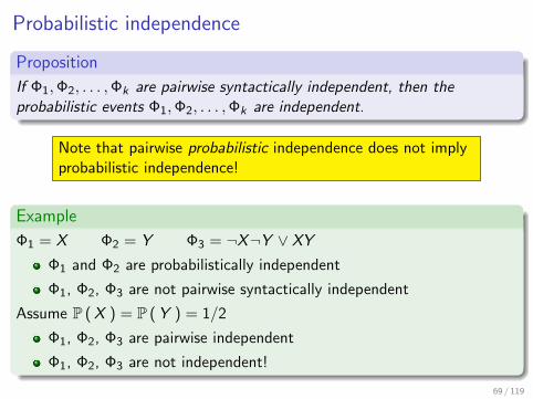
Probabilistic independence
Proposition
If Φ1,Φ2, . . . ,Φk are pairwise syntactically independent, then theprobabilistic events Φ1,Φ2, . . . ,Φk are independent.
Note that pairwise probabilistic independence does not implyprobabilistic independence!
Example
Φ1 = X Φ2 = Y Φ3 = ¬X¬Y ∨ XY
Φ1 and Φ2 are probabilistically independent
Φ1, Φ2, Φ3 are not pairwise syntactically independent
Assume P ( X ) = P ( Y ) = 1/2
Φ1, Φ2, Φ3 are pairwise independent
Φ1, Φ2, Φ3 are not independent!
69 / 119

Outline
1 Primer: Relational Calculus
2 The Query Evaluation Problem
3 Extensional Query EvaluationSyntactic IndependenceSix Simple RulesTractability and CompletenessExtensional Plans
4 Intensional Query EvaluationSyntactic independence5 Simple RulesQuery CompilationApproximation Techniques
5 Summary
70 / 119

Rules 1 and 2: independent-and, independent-or
Definition
Let Φ1 and Φ2 be two syntactically independent propositional formulas:
P ( Φ1 ∧ Φ2 ) = P ( Φ1 ) · P ( Φ2 ) (independent-and)P ( Φ1 ∨ Φ2 ) = 1− (1− P ( Φ1 ))(1− P ( Φ2 )) (independent-or)
71 / 119
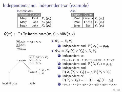
Independent-and, independent-or (example)IncriminatesWitness Suspect
Mary Paul X1 (p1)Mary John X2 (p2)Susan John X3 (p3)
AlibiSuspect Claim
Paul Cinema Y1 (q1)Paul Friend Y2 (q2)John Bar Y3 (q3)
Q(w)← ∃s.∃x .Incriminates(w , s) ∧ Alibi(s, x)
πWitness
onSuspect
Incriminates
πSuspect
Alibi
M X1(Y1 ∨ Y2) ∨ X2Y3
S X3Y3
M P X1(Y1 ∨ Y2)M J X2Y3
S J X3Y3
P Y1 ∨ Y2
J Y3
ΦS = X3Y3
1 Independent-and: P ( ΦS ) = p3q3
ΦM = X1(Y1 ∨ Y2) ∨ X2Y3
1 Independent-or:P ( ΦM ) = 1− (1− P ( X1(Y1 ∨ Y2) ))(1− P ( X2Y3 ))
2 Independent-and: P ( X2Y3 ) = p2q3
3 Independent-and:P ( X1(Y1 ∨ Y2) ) = p1 P ( Y1 ∨ Y2 )
4 Independent-or:P ( Y1 ∨ Y2 ) = 1− (1− q1)(1− q2)
5 P ( ΦM ) = 1− [1− p1(1− (1− q1)(1− q2))](1− p2q3)
72 / 119

Rule 3: Disjoint-or
Definition
Two propositional formulas Φ1 and Φ2 are disjoint if Φ1 ∧ Φ2 is notsatisfiable.
Definition
If Φ1 and Φ2 are disjoint:P ( Φ1 ∨ Φ2 ) = P ( Φ1 ) + P ( Φ2 ) (disjoint-or)
Example
P ( X ) = 0.2; P ( Y ) = 0.7
Φ1 = XY ; P ( XY ) = P ( X )P ( Y ) = 0.14
Φ2 = ¬X ; P (¬X ) = 0.8
P ( Φ1 ∨ Φ2 ) = P ( Φ1 ) + P ( Φ2 ) = 0.94
Checking for disjointness is NP-complete in general. Butdisjoint-or will play a major role for Shannon expansion.
73 / 119

Rule 4: Negation
Definition
P (¬Φ ) = 1− P ( Φ ) (negation)
Example
P ( X ) = 0.2; P ( Y ) = 0.7
P ( XY ) = P ( X )P ( Y ) = 0.14
P (¬(XY ) ) = 1− 0.14 = 0.86
74 / 119

Shannon expansion
Definition
The Shannon expansion of a propositional formula Φ w.r.t. a variable Xwith domain { a1, . . . , am } is given by:
Φ ≡ (Φ[X 7→ a1] ∧ (X = a1)) ∨ . . . ∨ (Φ[X 7→ am] ∧ (X = am))
Example
Φ = XY ∨ XZ ∨ YZ
Φ ≡ (Φ[X 7→ TRUE] ∧ X ) ∨ (Φ[X 7→ FALSE] ∧ ¬X )= (Y ∨ Z )X ∨ YZ¬X
In the Shannon expansion rule, every ∧ is an independent-and;every ∨ is a disjoint-or.
75 / 119

Rule 5: Shannon expansion
Definition
Let Φ be a propositional formula and X be a variable:
P ( Φ ) =∑
a∈dom(X )
P ( Φ[X 7→ a] )P ( X = a ) (Shannon expansion)
Example
Φ = XY ∨ XZ ∨ YZ
P ( Φ ) = P ( Y ∨ Z )P ( X ) + P ( YZ )P (¬X )
Can always be applied
Effectively eliminates X from the formula
But may lead to exponential blowup!
76 / 119

Shannon expansion (example)IncriminatesWitness Suspect
Mary Paul X1 (p1)Mary John X2 (p2)Susan John X3 (p3)
AlibiSuspect Claim
Paul Cinema Y1 (q1)Paul Friend Y2 (q2)John Bar Y3 (q3)
Q(w)← ∃s.∃x .Incriminates(w , s) ∧ Alibi(s, x)
πWitness
onSuspect
Incriminates Alibi
M X1Y1 ∨ X1Y2 ∨ X2Y3
S X3Y3
M P C X1Y1
M P F X1Y2
M J B X2Y3
S J B X3Y3
ΦM = X1Y1 ∨ X1Y2 ∨ X2Y31 Independent-or:
P ( ΦM ) = 1− (1− P (X1Y1 ∨ X1Y2 ))(1− P (X2Y3 ))
2 Independent-and: P ( X2Y3 ) = p2q3
3 Shannon expansion: P ( X1Y1 ∨ X1Y2) ) =P ( Y1 ∨ Y2 )P ( X1 ) + P ( FALSE )P (¬X1 )
4 Independent-or:P ( Y1 ∨ Y2 ) = 1− (1− q1)(1− q2)
5 P ( ΦM ) = 1− [1− p1(1− (1− q1)(1− q2))](1− p2q3)
The intensional rules work on all plans!
77 / 119
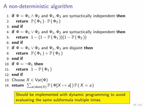
A non-deterministic algorithm
1: if Φ = Φ1 ∧ Φ2 and Φ1,Φ2 are syntactically independent then2: return P ( Φ1 ) · P ( Φ2 )3: end if4: if Φ = Φ1 ∨ Φ2 and Φ1,Φ2 are syntactically independent then5: return 1− (1− P ( Φ1 ))(1− P ( Φ2 ))6: end if7: if Φ = Φ1 ∨ Φ2 and Φ1,Φ2 are disjoint then8: return P ( Φ1 ) + P ( Φ2 )9: end if
10: if Φ = ¬Φ1 then11: return 1− P ( Φ1 )12: end if13: Choose X ∈ Var(Φ)14: return
∑a∈dom(X ) P ( Φ[X 7→ a] )P ( X = a )
Should be implemented with dynamic programming to avoidevaluating the same subformula multiple times.
78 / 119
Outline
1 Primer: Relational Calculus
2 The Query Evaluation Problem
3 Extensional Query EvaluationSyntactic IndependenceSix Simple RulesTractability and CompletenessExtensional Plans
4 Intensional Query EvaluationSyntactic independence5 Simple RulesQuery CompilationApproximation Techniques
5 Summary
79 / 119

Materialized views in TID databases (1)
TID databases complete only with viewsHow to deal with views in a PDBMS?
1 Store just the view definition2 Store the view result and probabilities3 Store the view result and lineage4 Store the view results and “compiled lineage”
Trade-off between precomputation and query cost (just as in DBMS)
Example (ExpensiveHotel view)q(h)← ∃n.∃c.Hotel(h, n, c) ∧ ∃r .∃t.∃p.Room(r , h, t, p) ∧ (p > 500 ∨ t = ’suite’)
Room (R)
RoomNo Type HotelNo PriceR1 Suite H1 $50 X1
R2 Single H1 $600 X2
R3 Double H1 $80 X3
Hotel (H)
HotelNo Name CityH1 Hilton SB X4
ExpensiveHotels
HotelNoH1 0.375
ExpensiveHotels
HotelNoH1 X4 ∧ (X1 ∨ X2)
ExpensiveHotels
HotelNoH1 X4 ∧i (X1 ∨i X2)
(2) (3) (4)80 / 119

Materialized views in TID databases (2)
Example (Continued)
Consider the query
q(h)← ∃c .ExpensiveHotel(h),Hotel(h, ’Hilton’, c),
which asks for expensive Hilton hotels using a view. Can we answer thisquery when ExpensiveHotel is a precomputed materialized view?
ExpensiveHotels
HotelNoH1 X4 ∧ (X1 ∨ X2)
ExpensiveHotels
HotelNoH1 0.375
ExpensiveHotels
HotelNoH1 X4 ∧i (X1 ∨i X2)
Yes, combine lineages No, dependencybetweenExpensiveHotels andHotels lost
Yes, combine “compiledlineages” → Need to beable to combine compiledlineages efficiently!
ExpensiveHiltons
HotelNoH1 [X4 ∧ (X1 ∨ X2)] ∧ X4
ExpensiveHiltons
HotelNoH1 X4 ∧i (X1 ∨ X2)
81 / 119
Hotel (H)
HotelNo Name CityH1 Hilton SB X4

Query compilation
“Compile” Φ into a Boolean circuit with certain desirable properties
P ( Φ ) can be computed in linear time in the size of the circuit
I Many other tasks can be solved in polynomial timeI E.g., combining formulas Φ1 ∧ Φ2 (even when not independent!)I Key application in PDBMS: Compile materialized views
Tractable compilation = circuit of size polynomial in database→ Implies tractable computation of P ( Φ ) (converse may not be true)
Compilation targets1 RO (read-once formula)2 OBDD (ordered binary decision diagram)3 FBDD (free binary decision diagram)4 d-DNF (deterministic-decomposable normal form)
Goals: (1) Reusability. (2) Understand complexity of intensional QE.
82 / 119

Restricted Boolean circuit (RBC)
Rooted, labeled DAG
All variables are Boolean
Each node (called gate) representents a propositional formula Ψ
Let Ψ be represented by a gate with children representing Ψ1, . . . ,Ψn;we consider the following gates & restrictions:
I Independent-and (∧i): Ψ1, . . . ,Ψn are syntactically independentI Independent-or (∨i): Ψ1, . . . ,Ψn syntactically independentI Disjoint-or (∨d): Ψ1, . . . ,Ψn are disjointI Not (¬): single child, represents ¬ΨI Conditional gate (X ): two children representing X ∧Ψ1 and ¬X ∧Ψ2,
where X /∈ Var(Ψ1) and X /∈ Var(Ψ2)I Leaf node (0, 1, X ): represents FALSE, TRUE, X
The different compilation targets restrict which and wheregates may be used.
83 / 119

Restricted Boolean circuit (example)
Example
Who incriminates someone who has an alibi?Lineage of unsafe plan: ΦM = X1Y1 ∨ X1Y2 ∨ X2Y3
∨i
X1
0
0
∨i
Y1 Y2
1
∧i
X2 Y3
“Documents” the non-deterministic algorithm for intensionalquery evaluation.
84 / 119

Deterministic-decomposable normal form (d-DNF)
Restricted to gates: ∧i, ∨d, ¬I ∧i-gates are called decomposable (D)I ∨d-gates are called deterministic (d)
Example
Φ = XYU ∨ XYZ¬U
∨d
∧i ∧i
X Y Z U ¬
85 / 119
RBC and d-DNF
Theorem
Every RBC with n gates can be transformed into an equivalent d-DNFwith at most 5n gates, a polynomial increase in size.
Proof.
We are not allowed to use ∨i and conditional nodes. Apply thetransformations:
∨i
Ψ1 Ψ2
→
¬
∧i
¬
Ψ1
¬
Ψ2
X
Ψ1
0
Ψ2
1→
∨d
∧i
¬
X
Ψ1
∧i
Ψ2
A ∨i-node is replaced by 4 new nodes. A conditional node is replaced by(at most) 5 new nodes.
86 / 119

Application: knowledge compilation
Tries to deal with intractability of propositional reasoningKey idea
1 Slow offline phase: Compilation into a target language2 Fast online phase: Answers in polynomial time
→ Offline cost amortizes over many online queriesKey aspects
I Succinctness of target language (d-DNF, FBDD, OBDD, ...)I Class of queries that can be answered efficiently once compiled
(consistency, validity, entailment, implicants, equivalence, modelcounting, probability computation, ...)
I Class of transformations that can be performed efficiently oncecompiled (∧, ∨, ¬, conditioning, forgetting, ...)
How to pick a target language?1 Identify which queries/transformations are needed2 Pick the most succinct language
Which queries admit polynomial representation in which target language?
87 / 119Darwiche and Marquis, 2002

Free binary decision diagram (FBDD)
Restricted to conditional gatesBinary decision diagram: Each node decides on the value of a variableFree: Each variable occurs only on every root-leaf path
Example
Who incriminates someone who has an alibi?Lineage of safe plan: ΦM = X1(Y1 ∨ Y2) ∨ X2Y3
X1
Y1
Y2
X2
Y3
0 1
1
0
1
0
1
0
1
0
0 1
88 / 119

Ordered binary decision diagram (OBDD)
An ordered FBDD, i.e.,I Same ordering of variables on each root-leaf pathI Omissions are allowed
Example
The FBDD on slide 88 is an OBDD with ordering X1,Y1,Y2,X2,Y3.
Theorem
Given two ODDBs Ψ1 and Ψ2 with a common variable order, we cancompute an ODDB for Ψ1 ∧Ψ2, Ψ1 ∨Ψ2, or ¬Ψ1 in polynomial time.Note that Ψ1 and Ψ2 do not need to be independent or disjoint.
(Many other results of this kind exist. Many BDD software packages exist,e.g., BuDDy, JDD, CUDD, CAL).
89 / 119
Read-once formulas (RO)
Definition
A propositional formula Φ is read-once (or repetition-free) if there exists aformula Φ′ such that Φ ≡ Φ′ and every variable occurs at most once in Φ′.
Example
Φ = X1 ∨ X2 ∨ X3 → read-once
Φ = X1Y1 ∨ X1Y2 ∨ X2Y3 ∨ X2Y4 ∨ X2Y5
I Φ′ = X1(Y1 ∨ Y2) ∨ X2(Y3 ∨ Y4 ∨ Y5) → read-once
Φ = XY ∨ XU ∨ YU → not read-once
Theorem
If Φ is given as a read-once formula, we can compute P ( Φ ) in linear time.
Proof.
All ∧’s and ∨’s are independent, and negation is easily handled.
90 / 119

When is a formula read-once? (1)
Definition
Let Φ be given in DNF such that no conjunct is a strict subset of someother conjunct. Φ is unate if every propositional variable X occurs eitheronly positively or negatively. The primal graph G (V ,E ) where V is the setof propositional variables in Φ and there is an edge (X ,Y ) ∈ E if X and Yoccur together in some conjunct.
Example
Unate: XY ∨ ¬ZX
Not unate: XY ∨ Z¬X
XU ∨ XV ∨ YU ∨ YV XY ∨ YU ∨ UV XY ∨ XU ∨ YU
X
Y
U
V
X
Y
U
V
X
Y
U
91 / 119

When is a formula read-once? (2)
Definition
A primal graph G for Φ is P4-free if no induced subgraph is isomorphic toP4 ( ). G is normal if for every clique in G , there is a conjunctin Φ that contains all of the clique’s variables.
Example
XU ∨ XV ∨ YU ∨ YV XY ∨ YU ∨ UV XY ∨ XU ∨ YU
X
Y
U
V
X
Y
U
V
X
Y
U
P4-free Not P4-free P4-freeNormal Normal Not normal
Read-once Not read-once Not read-once
Theorem
A unate formula is read-once iff it is P4-free and normal.92 / 119

Query compilation hierarchy
Denote by L (T ) the class of queries from L that can be compiledefficiently to target T . The following relationships hold for UCQ-queries:
93 / 119
Outline
1 Primer: Relational Calculus
2 The Query Evaluation Problem
3 Extensional Query EvaluationSyntactic IndependenceSix Simple RulesTractability and CompletenessExtensional Plans
4 Intensional Query EvaluationSyntactic independence5 Simple RulesQuery CompilationApproximation Techniques
5 Summary
94 / 119

Why approximation?
Exact inference may require exponential time → expensive
Often absolute probability values of little interest; ranking desired→ Good approximations of P ( Φ ) suffice
DesiderataI (Provably) low approximation errorI EfficientI Polynomial in database sizeI Anytime algorithm (gradual improvement)
ApproachesI Probability intervalsI Monte-Carlo approximation
We will show: Approximation is tractable forall RA-queries w.r.t. absolute error and for allUCQ-queries w.r.t. relative error!
95 / 119

Probability bounds
Theorem
Let Φ1 and Φ2 be propositional formulas. Then,
max(P ( Φ1 ) ,P ( Φ2 )) ≤ P ( Φ1 ∨ Φ2 ) ≤Boole’s inequality / union bound︷ ︸︸ ︷
min(P ( Φ1 ) + P ( Φ2 ) , 1)max(0,P ( Φ1 ) + P ( Φ2 )− 1)︸ ︷︷ ︸
via inclusion-exclusion
≤ P ( Φ1 ∧ Φ2 ) ≤ min(P ( Φ1 ) ,P ( Φ2 )).
Example
Border cases:P
Φ1
Φ2
P
Φ2
Φ1
P
Φ1 Φ2
P ( Φ1 ∨ Φ2 ) P ( Φ1 ) + P ( Φ2 ) P ( Φ2 ) 1P ( Φ1 ∧ Φ2 ) 0 P ( Φ1 ) P ( Φ1 ) + P ( Φ2 )− 1
96 / 119
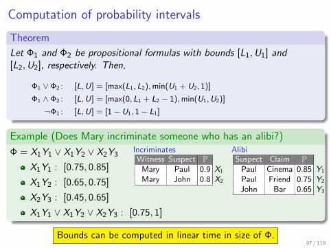
Computation of probability intervals
Theorem
Let Φ1 and Φ2 be propositional formulas with bounds [L1,U1] and[L2,U2], respectively. Then,
Φ1 ∨ Φ2 : [L,U] = [max(L1, L2),min(U1 + U2, 1)]
Φ1 ∧ Φ2 : [L,U] = [max(0, L1 + L2 − 1),min(U1,U2)]
¬Φ1 : [L,U] = [1− U1, 1− L1]
Example (Does Mary incriminate someone who has an alibi?)
Φ = X1Y1 ∨ X1Y2 ∨ X2Y3
X1Y1 : [0.75, 0.85]
X1Y2 : [0.65, 0.75]
X2Y3 : [0.45, 0.65]
X1Y1 ∨ X1Y2 ∨ X2Y3 : [0.75, 1]
Bounds can be computed in linear time in size of Φ.97 / 119
IncriminatesWitness Suspect P
Mary Paul 0.9 X1
Mary John 0.8 X2
AlibiSuspect Claim P
Paul Cinema 0.85 Y1
Paul Friend 0.75 Y2
John Bar 0.65 Y3
Probability intervals and intensional query evaluation
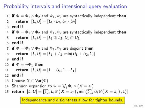
1: if Φ = Φ1 ∧ Φ2 and Φ1,Φ2 are syntactically independent then2: return [L,U] = [L1 · L2,U1 · U2]3: end if4: if Φ = Φ1 ∨ Φ2 and Φ1,Φ2 are syntactically independent then5: return [L,U] = [L1 ⊕ L2,U1 ⊕ U2]6: end if7: if Φ = Φ1 ∨ Φ2 and Φ1,Φ2 are disjoint then8: return [L,U] = [L1 + L2,min(U1 + U2, 1)]9: end if
10: if Φ = ¬Φ1 then11: return [L,U] = [1− U1, 1− L1]12: end if13: Choose X ∈ Var(Φ)14: Shannon expansion to Φ =
∨i Φi ∧ (X = ai )
15: return [L,U] = [∑
i Li P ( X = ai ) ,min(∑
i Ui P ( X = ai ) , 1)]
Independence and disjointness allow for tighter bounds.98 / 119

Probability intervals and intensional query evaluation (2)
ExampleIncriminatesWitness Suspect P
Mary Paul 0.9 X1
Mary John 0.8 X2
AlibiSuspect Claim P
Paul Cinema 0.85 Y1
Paul Friend 0.75 Y2
John Bar 0.65 Y3
Φ = X1Y1∨X1Y2∨X2Y3
X1Y1 : [0.75, 0.85]
X1Y2 : [0.65, 0.75]
X2Y3 : [0.45, 0.65]
Φ : [0.75, 1]
∨i
X1Y1 ∨ X1Y2 ∧i
X2 Y3
[0.88, 1]
[0.52, 0.52]
[0.8, 0.8] [0.65, 0.65]
[0.75, 1]
∨i
X1
F
0
Y1 ∨ Y2
1
∧i
X2 Y3
[0.8872, 0.952]
[0.52, 0.52]
[0.8, 0.8] [0.65, 0.65]
[0.765, 0.9]
[0.85, 1][0, 0]
99 / 119
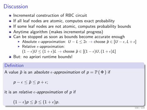
Discussion
Incremental construction of RBC circuitIf all leaf nodes are atomic, computes exact probabilityIf some leaf nodes are not atomic, computes probability boundsAnytime algorithm (makes incremental progress)Can be stopped as soon as bounds become accurate enough
I Absolute ε-approximation: U − L ≤ 2ε → choose p ∈ [U − ε, L + ε]I Relative ε-approximation:
(1− ε)U ≤ (1 + ε)L → choose p ∈ [(1− ε)U, (1 + ε)L]
But: no apriori runtime bounds!
Definition
A value p is an absolute ε-approximation of p = P ( Φ ) if
p − ε ≤ p ≤ p + ε;
it is an relative ε-approximation of p if
(1− ε)p ≤ p ≤ (1 + ε)p.100 / 119
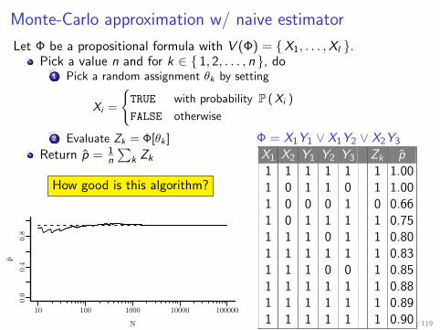
Monte-Carlo approximation w/ naive estimator
Let Φ be a propositional formula with V (Φ) = {X1, . . . ,Xl }.Pick a value n and for k ∈ { 1, 2, . . . , n }, do
1 Pick a random assignment θk by setting
Xi =
{TRUE with probability P ( Xi )
FALSE otherwise
2 Evaluate Zk = Φ[θk ]
Return p = 1n
∑k Zk
How good is this algorithm?
N
p
10 100 1000 10000 100000
0.0
0.4
0.8
101 / 119
Φ = X1Y1 ∨ X1Y2 ∨ X2Y3
X1 X2 Y1 Y2 Y3 Zk p1 1 1 1 1 1 1.001 0 1 1 0 1 1.001 0 0 0 1 0 0.661 0 1 1 1 1 0.751 1 1 0 1 1 0.801 1 1 1 1 1 0.831 1 1 0 0 1 0.851 1 1 1 1 1 0.881 1 1 1 1 1 0.891 1 1 1 1 1 0.90
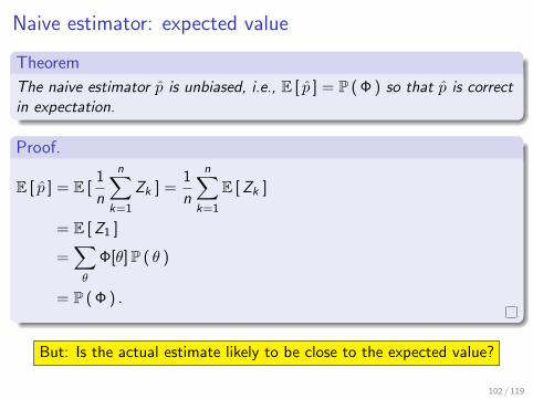
Naive estimator: expected value
Theorem
The naive estimator p is unbiased, i.e., E [ p ] = P ( Φ ) so that p is correctin expectation.
Proof.
E [ p ] = E [1
n
n∑k=1
Zk ] =1
n
n∑k=1
E [ Zk ]
= E [ Z1 ]
=∑θ
Φ[θ]P ( θ )
= P ( Φ ) .
But: Is the actual estimate likely to be close to the expected value?
102 / 119
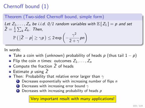
Chernoff bound (1)
Theorem (Two-sided Chernoff bound, simple form)
Let Z1, . . . ,Zn be i.i.d. 0/1 random variables with E [ Z1 ] = p and setZ = 1
n
∑k Zk . Then,
P( ∣∣Z − p
∣∣ ≥ γp)≤ 2 exp
(− γ2
2 + γpn
)In words:
Take a coin with (unknown) probability of heads p (thus tail 1− p)Flip the coin n times: outcomes Z1, . . . ,Zn
Compute the fraction Z of headsEstimate p using ZThen: Probability that relative error larger than γ
1 Decreases exponentially with increasing number of flips n2 Decreases with increasing error bound γ3 Decreases with increasing probability of heads p
Very important result with many applications!
103 / 119

Chernoff bound (2)
Theorem (Two-sided Chernoff bound, simple form)
Let Z1, . . . ,Zn be i.i.d. 0/1 random variables with E [ Z1 ] = p and setZ = 1
n
∑k Zk . Then,
P( ∣∣Z − p
∣∣ ≥ γp)≤ 2 exp
(− γ2
2 + γpn
)Proof (outline).
We give the first steps of the proof of the one-sided Chernoff bound. First,
P (Z ≥ q ) = P( etZ ≥ etq ).
for any t > 0. Use the Markov inequality P ( |X | ≥ a ) ≤ E [ |X | ]/a to obtain
P (Z ≥ q ) ≤ E [ etZ ]/etq
= E [ etZ1 · · · etZn ]/etq = E [ etZ1 ] · · ·E [ etZn ]/etq = E [ etZ1 ]n/etq
Use definition of expected value and find the value of t that minimizes RHS to obtainthe precise one-sided Chernoff bound. Relax the RHS to obtain the simple form.
104 / 119

Naive estimator: absolute (ε,δ)-approximation (1)
Theorem (sampling theorem)
To obtain an absolute ε-approximation with probability at least 1− δ, itsuffices to run
n ≥ 2 + ε
ε2ln
2
δ= O
(1
ε2ln
1
δ
)sampling steps.
Proof.
Take γ = ε/p and apply the Chernoff bound to obtain
P( ∣∣Z − p
∣∣ ≥ ε ) ≤ 2 exp
(− ε2/p2
2 + ε/ppn
)= 2 exp
(− ε2
2p + εn
)≤ 2 exp
(− ε2
2 + εn
)since p ≤ 1. Now solve RHS ≤ δ for n.
105 / 119
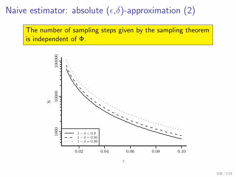
Naive estimator: absolute (ε,δ)-approximation (2)
The number of sampling steps given by the sampling theoremis independent of Φ.
ε
N
0.02 0.04 0.06 0.08 0.10
1000
10000
100000
1− δ = 0.91− δ = 0.951− δ = 0.99
106 / 119
Naive estimator: relative (ε,δ)-approximation (1)
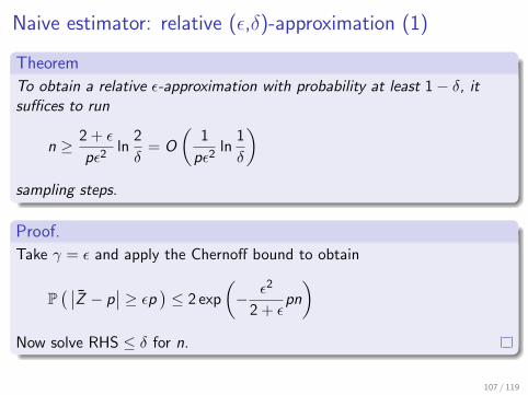
Theorem
To obtain a relative ε-approximation with probability at least 1− δ, itsuffices to run
n ≥ 2 + ε
pε2ln
2
δ= O
(1
pε2ln
1
δ
)sampling steps.
Proof.
Take γ = ε and apply the Chernoff bound to obtain
P( ∣∣Z − p
∣∣ ≥ εp ) ≤ 2 exp
(− ε2
2 + εpn
)Now solve RHS ≤ δ for n.
107 / 119

Naive estimator: relative (ε,δ)-approximation (2)
The number of sampling steps given by the sampling theorem now is de-pendent on Φ; we cannot compute the number of required steps in ad-vance! Obtaining small relative error for small p (i.e., Φ is often false)requires a large number of sampling steps.
ε
N
0.02 0.04 0.06 0.08 0.10
1000
10000
100000
1000000
p = 0.9p = 0.5p = 0.1p = 0.01
108 / 119
1− δ = 0.9

Why care about relative ε-approximation?1 Absolute error ill-suited to compare estimates of small probabilities
I p1 = 0.001, p2 = 0.01, ε = 0.1I Absolute error: I1 = [0, 0.101], I2 = [0, 0.11]I Relative error: I1 = [0.0009, 0.0011], I2 = [0.009, 0.011]
→ Ranking of tuples more sensitive to absolute error
2 For p ∈ [0, 1), relative error ε is always tighter than absolute error ε(esp. when probabilities are small)
Can we get a relative ε-approximation in which the minimumnumber of sampling steps does not depend on P ( Φ )?
109 / 119

The problem with the naive estimator
Φ = X1Y1 ∨ X1Y2 ∨ X2Y3
N
p
10 100 1000 10000 100000
0.0
0.4
0.8
N
p
10 100 1000 10000 1000000.00000
0.00010
0.00020
Large probabilities Small probabilities (×10−2)
When P ( Φ ) is small, Φ not satisfied on most samples→ Slow convergence
Idea: Change the sampling strategy so that Φ is satisfied onevery sample.
110 / 119

Karp-Luby estimator (basic idea)
Let Φ be a propositional DNF formula with V (Φ) = {X1, . . . ,Xl }, i.e.,
Φ = C1 ∨ C2 ∨ · · · ∨ Cm.Easy to find satisfying assignments!
Set qi = P ( Ci ) and Q =∑
i qi . Note that p ≤ Q (union bound).
P ( Φ ) = P ( C1 ) + P (¬C1 ∧ C2 ) + · · ·+ P (¬(C1 ∨ · · · ∨ Cm−1) ∧ Cm )
= P ( TRUE | C1 )P ( C1 ) + P (¬C1 | C2 )P ( C2 ) + · · ·+ P (¬(C1 ∨ · · · ∨ Cm−1) | Cm )P ( Cm )
= Q [P ( TRUE | C1 ) q1/Q + P (¬C1 | C2 ) q2/Q + · · ·+ P (¬(C1 ∨ · · · ∨ Cm−1) | Cm ) qm/Q]
Idea of Karp-Luby estimator:1 qi/Q is computed exactly (in linear time)2 P (¬(C1 ∨ · · · ∨ Ci−1) | Ci ) are estimated
I Impact of estimate proportional to P ( Ci )→ Focus on clauses with highest probability
111 / 119
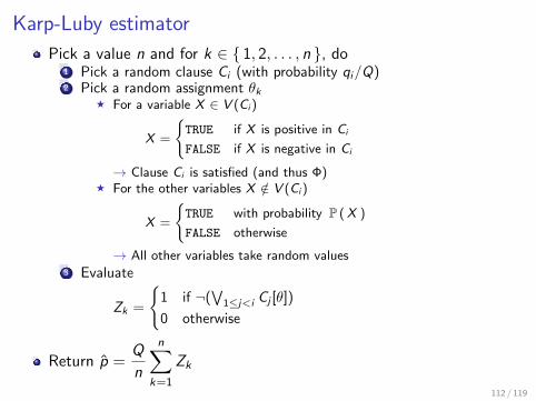
Karp-Luby estimator
Pick a value n and for k ∈ { 1, 2, . . . , n }, do1 Pick a random clause Ci (with probability qi/Q)2 Pick a random assignment θk
F For a variable X ∈ V (Ci )
X =
{TRUE if X is positive in Ci
FALSE if X is negative in Ci
→ Clause Ci is satisfied (and thus Φ)F For the other variables X /∈ V (Ci )
X =
{TRUE with probability P (X )
FALSE otherwise
→ All other variables take random values3 Evaluate
Zk =
{1 if ¬(
∨1≤j<i Cj [θ])
0 otherwise
Return p =Q
n
n∑k=1
Zk
112 / 119

Example of KL estimator
Φ = X1Y1 ∨ X1Y2 ∨ X2Y3
m = 3, probabilities of X1 and Y3 reduced to 1/10th
C1 = X1Y1, q1 = 0.09 · 0.85 = 0.0765, q1/Q ≈ 0.39
C2 = X1Y2, q2 = 0.09 · 0.75 = 0.0675, q2/Q ≈ 0.34
C3 = X2Y3, q3 = 0.8 · 0.065 = 0.052, q3/Q ≈ 0.27
Q = 0.196, p ≈ 0.134
i X1 X2 Y1 Y2 Y3 C1 C2 C3 Zk p1 1 1 1 1 0 1 1 0 1 0.1963 0 1 1 1 1 0 0 1 1 0.1962 1 1 1 1 0 1 1 0 0 0.1311 1 1 1 1 0 1 1 0 1 0.1471 1 1 1 1 0 1 1 0 1 0.1572 1 0 1 1 0 1 1 0 0 0.131
113 / 119

KL estimator: expected value
Theorem
The KL estimator p is unbiased, i.e., E [ p ] = P ( Φ ) so that p is correct inexpectation.
Proof.
E [ p ] = E [Q
n
n∑k=1
Zk ] = Q E [ Z1 ] = Q E [E [ Z1 | Ci picked ] ]
= Qm∑i=1
qi
QE [ Z1 | Ci picked ]
=m∑i=1
P ( Ci )P(¬∨
1≤j<i
Cj | Ci )
= P ( Φ ) .
114 / 119
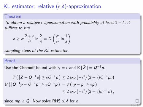
KL estimator: relative (ε,δ)-approximation
Theorem
To obtain a relative ε-approximation with probability at least 1− δ, itsuffices to run
n ≥ m2 + ε
ε2ln
2
δ= O
(m
ε2ln
1
δ
)sampling steps of the KL estimator.
Proof.
Use the Chernoff bound with γ = ε and E [ Z ] = Q−1p.
P( ∣∣Z − Q−1p
∣∣ ≥ εQ−1p)≤ 2 exp
(−ε2/(2 + ε)Q−1pn
)P( ∣∣Q−1p− Q−1p
∣∣ ≥ εQ−1p)
= P ( |p− p| ≥ εp )
≤ 2 exp(−ε2/(2 + ε)m−1n
),
since mp ≥ Q. Now solve RHS ≤ δ for n.115 / 119

KL estimator: discussion
KL estimator provides relative (ε,δ)-approximation in polynomial timein size of Φ and 1
ε→fully polynomial-time randomized approximation scheme (FPTRAS)
Example: Φ = X1Y1 ∨ X1Y2 ∨ X2Y3
N
p
10 100 1000 10000 100000
0.0
0.4
0.8
N
p
10 100 1000 10000 1000000.00000
0.00010
0.00020
Large probabilities Small probabilities (×10−2)Requires DNF (=why-provenance; polynomial in DB size for UCQ)
For ε, δ fixed and relative error, the naive estimator requires O(p−1) sam-pling steps and the KL estimator requires O(m) steps. In general, thenaive estimator is preferable when the DNF is very large. The KL estimatorpreferable if probabilities are small.
116 / 119

Outline
1 Primer: Relational Calculus
2 The Query Evaluation Problem
3 Extensional Query EvaluationSyntactic IndependenceSix Simple RulesTractability and CompletenessExtensional Plans
4 Intensional Query EvaluationSyntactic independence5 Simple RulesQuery CompilationApproximation Techniques
5 Summary
117 / 119
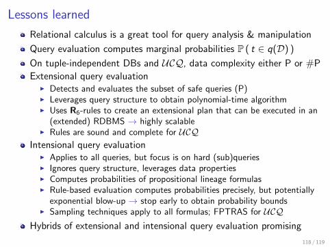
Lessons learned
Relational calculus is a great tool for query analysis & manipulation
Query evaluation computes marginal probabilities P ( t ∈ q(D) )
On tuple-independent DBs and UCQ, data complexity either P or #P
Extensional query evaluationI Detects and evaluates the subset of safe queries (P)I Leverages query structure to obtain polynomial-time algorithmI Uses R6-rules to create an extensional plan that can be executed in an
(extended) RDBMS → highly scalableI Rules are sound and complete for UCQ
Intensional query evaluationI Applies to all queries, but focus is on hard (sub)queriesI Ignores query structure, leverages data propertiesI Computes probabilities of propositional lineage formulasI Rule-based evaluation computes probabilities precisely, but potentially
exponential blow-up → stop early to obtain probability boundsI Sampling techniques apply to all formulas; FPTRAS for UCQ
Hybrids of extensional and intensional query evaluation promising
118 / 119

Suggested reading
Serge Abiteboul, Richard Hull, Victor VianuFoundations of Databases: The Logical Level (ch. 12)Addison Wesley, 1994
Dan Sucio, Dan Olteanu, Christopher Re, Christoph KochProbabilistic Databases (ch. 3–5)Morgan&Claypool, 2011
Michael Mitzenmacher, Eli UpfalProbability and Computing: Randomized Algorithms and ProbabilisticAnalysis (ch. 10)Cambridge University Press, 2005
119 / 119


