Scale-dependent growth from a transition in dark energy dynamics Mustafa A. Amin, * Phillip Zukin, † and Edmund Bertschinger ‡ Department of Physics and Kavli Institute for Astrophysics and Space Research Massachusetts Institute of Technology, Cambridge, Massachusetts 02139, USA (Received 11 August 2011; published 9 May 2012) We investigate the observational consequences of the quintessence field rolling to and oscillating near a minimum in its potential, if it happens close to the present epoch (z & 0:2). We show that in a class of models, the oscillations lead to a rapid growth of the field fluctuations and the gravitational potential on subhorizon scales. The growth in the gravitational potential occurs on time scales H 1 . This effect is present even when the quintessence parameters are chosen to reproduce an expansion history consistent with observations. For linearized fluctuations, we find that although the gravitational potential power spectrum is enhanced in a scale-dependent manner, the shape of the dark matter/galaxy power spectrum is not significantly affected. We find that the best constraints on such a transition in the quintessence field is provided via the integrated Sachs-Wolfe effect in the CMB-temperature power spectrum. Going beyond the linearized regime, the quintessence field can fragment into large, localized, long-lived excitations (oscillons) with sizes comparable to galaxy clusters; this fragmentation could provide additional observational constraints. Two quoted signatures of modified gravity are a scale-dependent growth of the gravitational potential and a difference between the matter power spectrum inferred from measure- ments of lensing and galaxy clustering. Here, both effects are achieved by a minimally coupled scalar field in general relativity with a canonical kinetic term. In other words we show that, with some tuning of parameters, scale-dependent growth does not necessarily imply a violation of General Relativity. DOI: 10.1103/PhysRevD.85.103510 PACS numbers: 98.80.k, 04.80.Cc I. INTRODUCTION Scalar fields are used ubiquitously in cosmology to provide a mechanism for accelerated expansion during both the inflationary [1–3] and current dark-energy domi- nated epochs (for example, [4–6]). In the inflationary case, accelerated expansion occurs when the inflaton field is rolling slowly and it ends once the field starts oscillating around the minimum of its potential. The oscillatory phase is well studied and gives rise to rapid growth of inhomo- geneities because of couplings to other fields or self- interactions (see, e.g. [7–10]). For a recent review, see [11]. Like the inflaton, the quintessence field provides a mechanism for accelerated expansion in the slow-roll re- gime. However, unlike inflation, the possibility of the accelerated expansion ending through quintessence oscil- lations is rarely discussed in the literature (however, see e.g. [12]). If quintessence was rolling slowly in the past, it is ‘‘natural’’ [though certainly not necessary] for it to enter an oscillatory regime as it finds its way towards a local minimum in its potential. In this paper, we wish to understand the observational signatures of a transition to an oscillatory regime in the quintessence field, if such a transition occurs in our recent past (z & 0:2). An obvious observational signature is a late-time change in expansion history. More importantly, as is the case with the inflaton, the coherent oscillations of quintessence near an anharmonic minimum are unstable and quickly fragment in a spatially inhomogeneous man- ner, giving rise to additional structure. This instability driven by self-interactions of the field (the anharmonic terms) leads to a growth in structure that is much faster than the usual gravitational growth. For example, all po- tentials that have a quadratic minimum and are shallower than quadratic away from the minimum (see Fig. 1) suffer from this instability (in particular for wave numbers k m, where m 2 U 00 ð’Þj ’!0 . See, for e.g [9,13–15]). We find that while the gravitational potential is influenced strongly by such growth in the quintessence fluctuations, the overdensity in baryons and dark matter does not change significantly. The scale-dependent growth in the gravita- tional potential and the absence of similar growth in the matter power spectrum provides a signature to confirm or rule out such a transition in the dynamics of the quintes- sence field. In addition, if the quintessence field becomes nonlinear, it can fragment rapidly into long-lived, localized excitations called oscillons (see e.g. [9,15–32]) with size l few m 1 few Mpc. 1 Although we do not pur- sue this in detail in this paper, in Appendix B, we comment on how such rapid nonlinear fragmentation of the field, and to a lesser extent, the time-dependent evolution of oscillon * [email protected]† [email protected]‡ [email protected]1 We will frequently relate the mass of the scalar field m, to length and time scales, without explicitly writing ℏ and c. We set ℏ ¼ c ¼ 1 throughout the paper. PHYSICAL REVIEW D 85, 103510 (2012) 1550-7998= 2012=85(10)=103510(20) 103510-1 Ó 2012 American Physical Society
Transcript
Scale-dependent growth from a transition in dark energy dynamics
Mustafa A. Amin,* Phillip Zukin,† and Edmund Bertschinger‡
Department of Physics and Kavli Institute for Astrophysics and Space Research Massachusetts Institute of Technology,Cambridge, Massachusetts 02139, USA
(Received 11 August 2011; published 9 May 2012)
We investigate the observational consequences of the quintessence field rolling to and oscillating near a
minimum in its potential, if it happens close to the present epoch (z & 0:2). We show that in a class of
models, the oscillations lead to a rapid growth of the field fluctuations and the gravitational potential on
subhorizon scales. The growth in the gravitational potential occurs on time scales � H�1. This effect is
present even when the quintessence parameters are chosen to reproduce an expansion history consistent
with observations. For linearized fluctuations, we find that although the gravitational potential power
spectrum is enhanced in a scale-dependent manner, the shape of the dark matter/galaxy power spectrum is
not significantly affected. We find that the best constraints on such a transition in the quintessence field is
provided via the integrated Sachs-Wolfe effect in the CMB-temperature power spectrum. Going beyond
the linearized regime, the quintessence field can fragment into large, localized, long-lived excitations
(oscillons) with sizes comparable to galaxy clusters; this fragmentation could provide additional
observational constraints. Two quoted signatures of modified gravity are a scale-dependent growth of
the gravitational potential and a difference between the matter power spectrum inferred from measure-
ments of lensing and galaxy clustering. Here, both effects are achieved by a minimally coupled scalar field
in general relativity with a canonical kinetic term. In other words we show that, with some tuning of
parameters, scale-dependent growth does not necessarily imply a violation of General Relativity.
Scalar fields are used ubiquitously in cosmology toprovide a mechanism for accelerated expansion duringboth the inflationary [1–3] and current dark-energy domi-nated epochs (for example, [4–6]). In the inflationary case,accelerated expansion occurs when the inflaton field isrolling slowly and it ends once the field starts oscillatingaround the minimum of its potential. The oscillatory phaseis well studied and gives rise to rapid growth of inhomo-geneities because of couplings to other fields or self-interactions (see, e.g. [7–10]). For a recent review, see[11]. Like the inflaton, the quintessence field provides amechanism for accelerated expansion in the slow-roll re-gime. However, unlike inflation, the possibility of theaccelerated expansion ending through quintessence oscil-lations is rarely discussed in the literature (however, seee.g. [12]). If quintessence was rolling slowly in the past, itis ‘‘natural’’ [though certainly not necessary] for it to enteran oscillatory regime as it finds its way towards a localminimum in its potential.
In this paper, we wish to understand the observationalsignatures of a transition to an oscillatory regime in thequintessence field, if such a transition occurs in our recentpast (z & 0:2). An obvious observational signature is alate-time change in expansion history. More importantly,
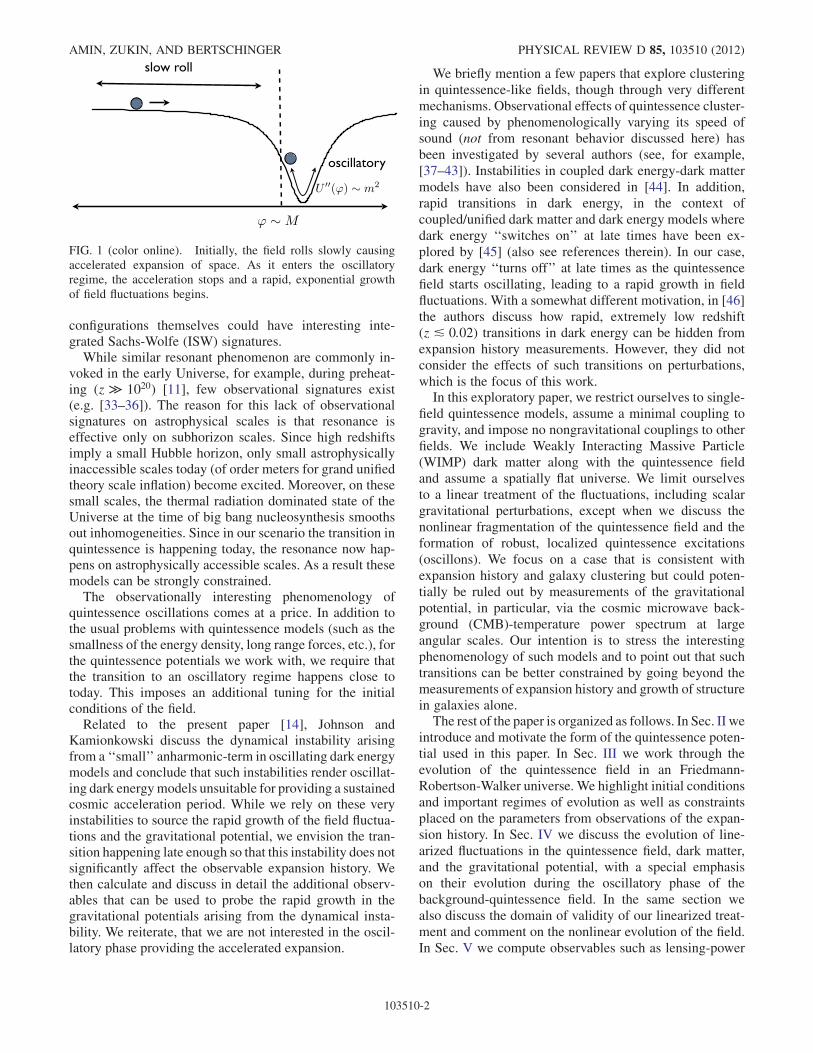
as is the case with the inflaton, the coherent oscillations ofquintessence near an anharmonic minimum are unstableand quickly fragment in a spatially inhomogeneous man-ner, giving rise to additional structure. This instabilitydriven by self-interactions of the field (the anharmonicterms) leads to a growth in structure that is much fasterthan the usual gravitational growth. For example, all po-tentials that have a quadratic minimum and are shallowerthan quadratic away from the minimum (see Fig. 1) sufferfrom this instability (in particular for wave numbersk � m, where m2 � U00ð’Þj’!0. See, for e.g [9,13–15]).
We find that while the gravitational potential is influencedstrongly by such growth in the quintessence fluctuations,the overdensity in baryons and dark matter does not changesignificantly. The scale-dependent growth in the gravita-tional potential and the absence of similar growth in thematter power spectrum provides a signature to confirm orrule out such a transition in the dynamics of the quintes-sence field. In addition, if the quintessence field becomesnonlinear, it can fragment rapidly into long-lived, localizedexcitations called oscillons (see e.g. [9,15–32]) with sizel� few�m�1 � few�Mpc.1 Although we do not pur-sue this in detail in this paper, in Appendix B, we commenton how such rapid nonlinear fragmentation of the field, andto a lesser extent, the time-dependent evolution of oscillon
1We will frequently relate the mass of the scalar field m, tolength and time scales, without explicitly writing ℏ and c. We setℏ ¼ c ¼ 1 throughout the paper.
PHYSICAL REVIEW D 85, 103510 (2012)
1550-7998=2012=85(10)=103510(20) 103510-1 � 2012 American Physical Society
configurations themselves could have interesting inte-grated Sachs-Wolfe (ISW) signatures.
While similar resonant phenomenon are commonly in-voked in the early Universe, for example, during preheat-ing (z � 1020) [11], few observational signatures exist(e.g. [33–36]). The reason for this lack of observationalsignatures on astrophysical scales is that resonance iseffective only on subhorizon scales. Since high redshiftsimply a small Hubble horizon, only small astrophysicallyinaccessible scales today (of order meters for grand unifiedtheory scale inflation) become excited. Moreover, on thesesmall scales, the thermal radiation dominated state of theUniverse at the time of big bang nucleosynthesis smoothsout inhomogeneities. Since in our scenario the transition inquintessence is happening today, the resonance now hap-pens on astrophysically accessible scales. As a result thesemodels can be strongly constrained.
The observationally interesting phenomenology ofquintessence oscillations comes at a price. In addition tothe usual problems with quintessence models (such as thesmallness of the energy density, long range forces, etc.), forthe quintessence potentials we work with, we require thatthe transition to an oscillatory regime happens close totoday. This imposes an additional tuning for the initialconditions of the field.
Related to the present paper [14], Johnson andKamionkowski discuss the dynamical instability arisingfrom a ‘‘small’’ anharmonic-term in oscillating dark energymodels and conclude that such instabilities render oscillat-ing dark energymodels unsuitable for providing a sustainedcosmic acceleration period. While we rely on these veryinstabilities to source the rapid growth of the field fluctua-tions and the gravitational potential, we envision the tran-sition happening late enough so that this instability does notsignificantly affect the observable expansion history. Wethen calculate and discuss in detail the additional observ-ables that can be used to probe the rapid growth in thegravitational potentials arising from the dynamical insta-bility. We reiterate, that we are not interested in the oscil-latory phase providing the accelerated expansion.
We briefly mention a few papers that explore clusteringin quintessence-like fields, though through very differentmechanisms. Observational effects of quintessence cluster-ing caused by phenomenologically varying its speed ofsound (not from resonant behavior discussed here) hasbeen investigated by several authors (see, for example,[37–43]). Instabilities in coupled dark energy-dark mattermodels have also been considered in [44]. In addition,rapid transitions in dark energy, in the context ofcoupled/unified dark matter and dark energy models wheredark energy ‘‘switches on’’ at late times have been ex-plored by [45] (also see references therein). In our case,dark energy ‘‘turns off’’ at late times as the quintessencefield starts oscillating, leading to a rapid growth in fieldfluctuations. With a somewhat different motivation, in [46]the authors discuss how rapid, extremely low redshift(z & 0:02) transitions in dark energy can be hidden fromexpansion history measurements. However, they did notconsider the effects of such transitions on perturbations,which is the focus of this work.In this exploratory paper, we restrict ourselves to single-
field quintessence models, assume a minimal coupling togravity, and impose no nongravitational couplings to otherfields. We include Weakly Interacting Massive Particle(WIMP) dark matter along with the quintessence fieldand assume a spatially flat universe. We limit ourselvesto a linear treatment of the fluctuations, including scalargravitational perturbations, except when we discuss thenonlinear fragmentation of the quintessence field and theformation of robust, localized quintessence excitations(oscillons). We focus on a case that is consistent withexpansion history and galaxy clustering but could poten-tially be ruled out by measurements of the gravitationalpotential, in particular, via the cosmic microwave back-ground (CMB)-temperature power spectrum at largeangular scales. Our intention is to stress the interestingphenomenology of such models and to point out that suchtransitions can be better constrained by going beyond themeasurements of expansion history and growth of structurein galaxies alone.The rest of the paper is organized as follows. In Sec. II we
introduce and motivate the form of the quintessence poten-tial used in this paper. In Sec. III we work through theevolution of the quintessence field in an Friedmann-Robertson-Walker universe. We highlight initial conditionsand important regimes of evolution as well as constraintsplaced on the parameters from observations of the expan-sion history. In Sec. IV we discuss the evolution of line-arized fluctuations in the quintessence field, dark matter,and the gravitational potential, with a special emphasison their evolution during the oscillatory phase of thebackground-quintessence field. In the same section wealso discuss the domain of validity of our linearized treat-ment and comment on the nonlinear evolution of the field.In Sec. V we compute observables such as lensing-power
FIG. 1 (color online). Initially, the field rolls slowly causingaccelerated expansion of space. As it enters the oscillatoryregime, the acceleration stops and a rapid, exponential growthof field fluctuations begins.
AMIN, ZUKIN, AND BERTSCHINGER PHYSICAL REVIEW D 85, 103510 (2012)
103510-2
spectra and the integrated Sachs-Wolfe (ISW) contributionto the CMB-temperature anisotropy. We present ourconclusions in Sec. VI. We also include two Appendixes.In Appendix A, we provide some details of Floquet analysisand an algorithm used in this paper for calculating Floquetexponents. In Appendix B, we provide an estimate of theISW effect resulting from evolution of quasi/nonlinearquintessence fluctuations and oscillons.
II. THE MODEL
We consider a quintessence field governed by a potentialof the form (see Fig. 1):
Uð’Þ ¼ m2M2
2
� ð’=MÞ21þ ð’=MÞ2ð1��Þ
�; (1)
where 0<�< 1.2 This choice was motivated by monod-romy and supergravity models of inflation [47–51] and arecent model of axion quintessence [52] (� ¼ 1=2). Thepotential has a quadratic minimum and for very large fieldvalues it asymptotes to a shallower than quadratic form,
Uð’Þ � m2
2’2 ’ � M;
Uð’Þ � m2M2
2ð’=MÞ2� ’ � M:
(2)
The scaleM determines where the potential changes shape,whereas, the scale m determines the curvature U00ð0Þ at thebottom of the well. We will consider cases where thefield rolls slowly for ’ � M, behaving like dark energyand then enters an oscillatory regime with ’�M afterz� 0:2. When the field oscillates around the minimum, the‘‘opening up’’ of the potential
Uð’Þ � ð1=2Þm2’2 < 0 ’ � 0; (3)
leads to rapid, scale-dependent growth of scalar-field fluc-tuations via parametric resonance (see Sec. IV). In thenonlinear regimes, it leads to the formation of localizedfield excitations called oscillons [9,29].
Similar phenomenology can arise in models such aspseudo-Nambu-Goldston-Boson quintessence (e.g. [53])
Uð’Þ ¼ m2M2½1� cosð’=MÞ�: (4)
For potentials (1) and (4), a limited range of parameterswill reproduce the observed expansion history, allow for afew oscillations in the field close to today, and allow forrapid growth of structure. For the pseudo-Nambu-Goldston-Boson-like models, the slow-roll dynamics ofthe field necessary for accelerated expansion only occurif M�mpl (unless ’ ! �M). However, as we discuss in
Sec. IV, efficient resonance in an expanding universe re-quiresM � mpl. As a result we do not get rapid growth of
structure here, except in cases of extreme fine tuning of theinitial conditions and do not pursue this model any furtherin this paper.
For the potential in (1), we find the requirement of a fewoscillations close to today translates into
10 2H0 & M; m & 10�2mpl and � � 1: (5)
We study these constraints in more detail in the nextsection.Finally, we note that resonant growth of fluctuations also
arise when scalar fields oscillate in potentials with asym-metric minima
Uð’Þ � m2
2’2 þM
3’3 þ . . . ;
and is possible in potentials with a nonquadratic minimumor in potentials, which do not necessarily open up (thoughthe band of resonant wave numbers can be narrow). Thekey requirement is that there are anharmonic terms in thepotential that provide a time-varying, periodic frequency inthe equation of motion for the fluctuations.
III. HOMOGENEOUS EVOLUTION
In this section, we describe how to choose initial con-ditions for the background quintessence field and parame-ters in the potential so that the field both oscillates at latetimes and reproduces the observed expansion history. Wedo this by trying to match the �CDM expansion history.This is more restrictive than directly using observations butmakes the following discussion more transparent.The equations of motion for the homogeneous quintes-
sence field are
€’þ3H _’þU0ð’Þ¼0; H2¼ 1
3m2pl
�_’2
2þUð’Þ
�þH2
0
�dm
a3;
(6)
where �dm is the fraction of the critical energy density inWIMPs today, H is the Hubble parameter, and H0 is itsvalue today.3 The dot ‘‘:’’ stands for a derivative withrespect to cosmic time and the scale factor a ¼ 1 today.We ignore the contribution from radiation since we areonly interested in late times.Current observations are consistent with the quintes-
sence field behaving like a cosmological constant in therecent past [54]. During the matter-dominated epoch, it ismore difficult to place constraints on dark energy’s equa-tion of state because it is subdominant. For simplicity, weassume that the field’s equation of state satisfies w �ð _’2 � 2UÞ=ð _’2 þ 2UÞ � �1 (for z * 0:2), which occursif the slow-roll condition _’2 � U is satisfied. Imposingthat the energy density in the quintessence field duringmatter domination has the same order of magnitude asthe �� in �CDM, we find
2We write ’ instead of j’j to avoid clutter.
3We choose the subscript ‘‘dm’’ for WIMPs instead of themore usual m to avoid confusion with the mass of the scalar field
SCALE-DEPENDENT GROWTH FROM A TRANSITION IN . . . PHYSICAL REVIEW D 85, 103510 (2012)
103510-3
�m
H0
�2�’i
M
�2� � 6ð1��dmÞ
�mPl
M
�2; (7)
where ’i is the initial value of the field deep in the matter-dominated epoch. Note that for simplicity, we have as-sumed that ’i � M and later justify our assumption at theend of the analysis. Since we are only interested in scalingrelationships, we will ignore factors of order unity fromnow on. The above gives one constraint between parame-ters in the potential and the field’s initial conditions.
Imposing oscillations in the field at late times gives asecond constraint. To derive this, we solve Eq. (6) in theslow-roll, matter-dominated regime, assuming the fielddoes not change significantly from its initial value. Wefind (assuming ’i � M)4
’
M�’i
M���a3ðm=H0Þ2ðM=’iÞ3 if �¼0;
�a3ðm=H0Þ2ðM=’iÞ1�2�� if �>0:(8)
Though the above equation of motion is not valid in theoscillation regime, it gives an approximate scale factor ðaÞwhen oscillations begin (’=M� 0). We find,
a �( ðH0=mÞ2=3ð’i=MÞ4=3 if � ¼ 0;
ðH0=mÞ2=3ð’i=MÞ2�2�=3��ð1=3Þ if �> 0:(9)
The actual scale factor when oscillations begin (aosc)differs from a, but the two are monotonically related.Combining Eqs. (7) and (9), we calculate explicit expres-sions for m and ’i in terms of M and a. We have
’i
M�
8<: a3=4 ðmpl=MÞ1=2 if � ¼ 0;
a3=4 ðmpl=MÞ�1=2 if � ¼ 0:
m
H0
�8<: ðmpl=MÞ if � ¼ 0;
a�3�=2 ðmpl=MÞ1����ð�=2Þ if � ¼ 0:
(10)
As discussed in more detail below in Sec. IV,M sets thestrength of the resonance between the perturbed quintes-sence field and the background quintessence field. Wetherefore keep it as a free parameter. We choose a sothat the actual numerically computed oscillations beginaround aosc � 0:8. Corrections to distance measurementsthat depend on cosmological parameters beyond H0 aresmall for scale factors larger than aosc � 0:8. Hence, mod-ifying the expansion history there will not interfere withmeasurements that probe the cosmological expansion.Finally, we fix m and ’i using Eq. (10). The value of _’i
follows from Eq. (8).In practice, when numerically evolving Eq. (6) accord-
ing to the above choices of initial conditions andpotential parameters, we find that in order to get agreementwith the �CDM expansion history in the past as well asproduce oscillations close to today, we require additional
fine-tuning of the initial conditions and parameters. Theprocedure described above results in a value of H0 that issmaller than the �CDM value. This is because by assump-tion, the Hubble parameter for both �CDM and quintes-sence are identical. At late times, however, the oscillationsin the quintessence field cause it to behave like dark matter,giving rise to a steeper falloff than the �CDM Hubbleparameter. For better agreement with H0, we increase thevalue of m until H0 agrees to better than a percent.Performing the above iteration, we find that � affects
whether or not the field starts oscillating at low redshift.This should be expected since the asymptotic slope of thepotential determines the time it takes to transition fromslow-roll to oscillations. We can calculate this approximatetime from the derivative of the quintessence field whenslow-roll ends. Using the slow-roll condition describedabove, the value of the quintessence field when slow-rollends is
’e �( ðmpl=MÞ1=3M if � ¼ 0;
�mpl if �> 0:(11)
Assuming 3H _’��U0, taking this transition to happenclose to today, and using the constraints in Eq. (10), we findthe change in scale factor (4 a) between the beginning ofoscillations (’� 0) and the end of slow-roll is given by
4a�( ðM=mplÞ2=3 if � ¼ 0;
�1�� if �> 0:(12)
The larger the �, the longer it takes for oscillations tostart. Hence, consistency with a �CDM-expansion historyand having late-time oscillations limits � � 1 for the caseof nonzero � andM � mpl for vanishing �. For the rest of
this paper, we specialize to� ¼ 0. In summary, we keepMand a as free parameters and choose m, ’i, and _’i so thatthe value of H0 agrees with the measured value, the fieldbehaves like dark energy initially, and the field startsoscillating at aosc � 0:8.For the above prescription, we calculate the evolution of
the quintessence field, the Hubble parameter normalizedby�CDM’s Hubble parameter, the field’s equation of stateparameter w, and the acceleration parameter q � €aa= _a2 asa function of scale factor. We show the results in Fig. 2 for
mpl=M ¼ 500; m=H0 ¼ 1130:6;
’i=M ¼ 23:7 with aosc ¼ 0:82:(13)
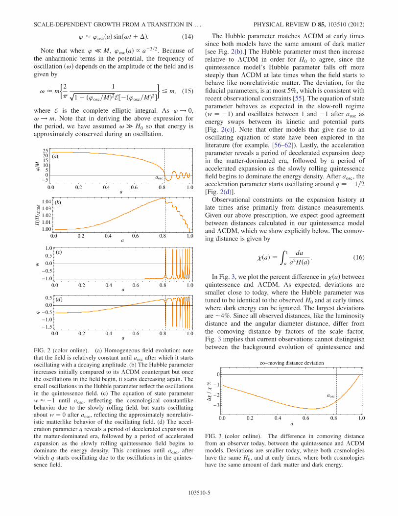
Unless otherwise stated we will use these as fiducial-parameter values throughout this paper and refer to themas fiducial parameters. As constructed, the field remainsapproximately constant for a � aosc, rolling slowlytowards the minimum. Notice, as assumed initially, that’ � M at early times. At aosc � 0:8, the field starts tooscillate with a slowly decaying amplitude
4The apparent discontinuity between the cases � ¼ 0 and�> 0 disappears when the full expressions are used.
AMIN, ZUKIN, AND BERTSCHINGER PHYSICAL REVIEW D 85, 103510 (2012)
103510-4
’ � ’oscðaÞ sinð!tþ �Þ: (14)
Note that when ’ � M, ’oscðaÞ / a�3=2. Because ofthe anharmonic terms in the potential, the frequency ofoscillation ð!Þ depends on the amplitude of the field and isgiven by
where E is the complete elliptic integral. As ’ ! 0,! ! m. Note that in deriving the above expression forthe period, we have assumed ! � H0 so that energy isapproximately conserved during an oscillation.
The Hubble parameter matches �CDM at early timessince both models have the same amount of dark matter[see Fig. 2(b).] The Hubble parameter must then increaserelative to �CDM in order for H0 to agree, since thequintessence model’s Hubble parameter falls off moresteeply than �CDM at late times when the field starts tobehave like nonrelativistic matter. The deviation, for thefiducial parameters, is at most 5%, which is consistent withrecent observational constraints [55]. The equation of stateparameter behaves as expected in the slow-roll regime(w ¼ �1) and oscillates between 1 and �1 after aosc asenergy swaps between its kinetic and potential parts[Fig. 2(c)]. Note that other models that give rise to anoscillating equation of state have been explored in theliterature (for example, [56–62]). Lastly, the accelerationparameter reveals a period of decelerated expansion deepin the matter-dominated era, followed by a period ofaccelerated expansion as the slowly rolling quintessencefield begins to dominate the energy density. After aosc, theacceleration parameter starts oscillating around q ¼ �1=2[Fig. 2(d)].Observational constraints on the expansion history at
late times arise primarily from distance measurements.Given our above prescription, we expect good agreementbetween distances calculated in our quintessence modeland �CDM, which we show explicitly below. The comov-ing distance is given by
�ðaÞ ¼Z 1
a
da
a2HðaÞ : (16)
In Fig. 3, we plot the percent difference in �ðaÞ betweenquintessence and �CDM. As expected, deviations aresmaller close to today, where the Hubble parameter wastuned to be identical to the observed H0 and at early times,where dark energy can be ignored. The largest deviationsare�4%. Since all observed distances, like the luminositydistance and the angular diameter distance, differ fromthe comoving distance by factors of the scale factor,Fig. 3 implies that current observations cannot distinguishbetween the background evolution of quintessence and
aosc
0.0 0.2 0.4 0.6 0.8 1.0
3
2
1
0
a
co moving distance deviation
FIG. 3 (color online). The difference in comoving distancefrom an observer today, between the quintessence and �CDMmodels. Deviations are smaller today, where both cosmologieshave the same H0, and at early times, where both cosmologieshave the same amount of dark matter and dark energy.
aosc
a
0.0 0.2 0.4 0.6 0.8 1.0
505
10152025
a
M
b
0.0 0.2 0.4 0.6 0.8 1.01.001.011.021.031.04
a
HH
CD
M
c
0.0 0.2 0.4 0.6 0.8 1.01.0
0.5
0.0
0.5
1.0
a
w
d
0.0 0.2 0.4 0.6 0.8 1.01.51.00.50.00.5
a
q
FIG. 2 (color online). (a) Homogeneous field evolution: notethat the field is relatively constant until aosc after which it startsoscillating with a decaying amplitude. (b) The Hubble parameterincreases initially compared to its �CDM counterpart but oncethe oscillations in the field begin, it starts decreasing again. Thesmall oscillations in the Hubble parameter reflect the oscillationsin the quintessence field. (c) The equation of state parameterw � �1 until aosc, reflecting the cosmological constantlikebehavior due to the slowly rolling field, but starts oscillatingabout w ¼ 0 after aosc, reflecting the approximately nonrelativ-istic matterlike behavior of the oscillating field. (d) The accel-eration parameter q reveals a period of decelerated expansion inthe matter-dominated era, followed by a period of acceleratedexpansion as the slowly rolling quintessence field begins todominate the energy density. This continues until aosc, afterwhich q starts oscillating due to the oscillations in the quintes-sence field.
SCALE-DEPENDENT GROWTH FROM A TRANSITION IN . . . PHYSICAL REVIEW D 85, 103510 (2012)
103510-5
the background evolution in �CDM [63–67]. We haverestricted our analysis to aosc � 0:8 because choosingaosc � 0:8 gives rise to unacceptably large deviationsfrom the observed expansion history.
IV. PERTURBATION EVOLUTION
In this section we investigate the dynamics of the fluc-tuations in the quintessence field (�’), the gravitationalpotentials, and the overdensity in WIMPs (�dm) assuminglinearized equations of motion. We ignore radiation andneutrinos, since we are interested in late-time dynamics.We work in the Newtonian gauge, where the metric is
ds2 ¼ �ð1þ 2�Þdt2 þ a2ð1� 2�Þdx2; (17)
and � and � are the two scalar-gravitational potentials.Tracking the evolution of the gravitational potentials andthe two matter components (WIMPs and quintessence)requires two second-order differential equations.Normally, they are taken to be the energy-momentumconservation equations for the matter components. Thegravitational potentials can then be obtained from theEinstein equations (constraints). However, since the mostinteresting dynamics happen in the gravitational potentialsand the field fluctuations, wework with them as the degreesof freedom and then obtain the overdensity inWIMPs fromthe constraints. The equations of motion for the quintes-sence field fluctuations and the gravitational potential are(in Fourier space)
€�’kþ3H _�’kþ�k2
a2þU00ð’Þ
��’k¼�2U0ð’Þ�kþ4 _’ _�k;
€�kþ4H _�kþ 1
m2pl
Uð’Þ�k¼ 1
2m2pl
½ _’ _�’k�U0ð’Þ�’k�:
(18)
The second equation is the diagonal, space-space compo-nent of the Einstein equations, where the right-hand side isthe pressure perturbation provided by the scalar field. Sincethe WIMP dark matter is assumed to be pressureless, itdoes not contribute to this source term. The second gravi-tational potential �k does not appear in the above equa-tions because there is no anisotropic stress at linear-orderfor single, minimally coupled scalar fields. This makes thetwo gravitational potentials equal
�k ¼ �k;
via the off-diagonal space-space part of the Einstein equa-tions.5 After evolving the equations for �’k and �k, �dm
follows from the time-time components of the Einsteinequations
�dm¼� a3
3H20�dm
��6H2� _’2
m2pl
þ2k2
a2
��kþ6H _�k
þ _’
m2pl
_�’kþ 1
m2pl
U0ð’Þ�’k
�: (19)
A. Initial conditions and evolution duringmatter domination
We are interested in the behavior of �’k, �k, and �dm
for a * 0:8. To solve (18) we need to specify �’k, � _’k,
�k,_�k on some initial time slice. This can be done self-
consistently using the �CDM solutions for �k and �dm ifthe initial time slice is chosen deep into the matter-dominated era. During matter domination, the quintes-sence field is a small fraction of the total energy density.As a result, the �’k do not contribute significantly to �k,and we can use�k from a�CDM cosmology at these early
times. We take these initial conditions for �k and _�k
directly from the output of CMBFAST [68] at ai � 10�2
since by this scale factor the anisotrotropic stress fromneutrinos is negligible and the contribution of dark energyis yet to become important. We are then left with specify-ing the initial conditions in �’k, which requires under-standing its evolution in the matter-dominated era.The evolution of adiabatic modes on superhorizon
k=aH � 1 scales is given by (see [69])
�’k ¼ �k
_’
H
� ðH=aÞRttiaðt0Þdt0
�1þ ðH=aÞRttiaðt0Þdt0
�: (20)
6 The term in the square brackets is constant during matterdomination
�’k ¼ � 2
3�k
_’
H: (21)
On subhorizon scales (k � aH), during the matter-dominated era, the gravitational potential is determinedby the fluctuations in the WIMP overdensity. Since �k
is constant during matter domination, the equations ofmotion (18) become
€�’ kþ3H _�’kþk2
a2�’k¼�2U0ð’Þ�k; _�k¼0; (22)
where we have assumedU00ð’Þ=H2 � ðk=aHÞ2. Under theassumption that U0ð’Þ is slowly varying, the completesolution is
fð’Þ�’k, where 8�GN ! fð’Þ�1. In minimally coupled fields,the anisotropic stress is generated by second-order terms�k ��k / �’2
k.6We will ignore isocurvature modes in this paper
AMIN, ZUKIN, AND BERTSCHINGER PHYSICAL REVIEW D 85, 103510 (2012)
103510-6
where kH � k=aH and ck, �k are constants of integrationset by initial conditions at the beginning of the matter-dominated era. For solutions that are deep inside thehorizon, kH � 1 and only one term grows with time
�’k � �2�k
U0ð’ÞH2
1
k2H: (24)
The initial (transient) oscillatory behavior due to the ho-mogeneous part of the solution (23) as well as the growth/ a2 for ai � a � aosc due to the particular solution (24)can be seen in Fig. 5(a). We have also verified that althoughfrom Eqs. (21) and (24) we see that �’k grows as a3 onsuperhorizon scales and as a2 on small, subhorizon scalestheir amplitude during matter domination does not becomelarge enough to change the behavior of the potential �k.
With Eqs. (21) and (24) at hand, we set the initialconditions for all kH, using a piecewise interpolation be-tween the subhorizon and superhorizon solutions (dashedcurve in Fig. 6). Although we have taken care to faithfullycharacterize the asymptotic behavior of the initial condi-tions of �’, in practice we find that changing the initialconditions by orders of magnitude does not affect ourresults significantly. This is because at late times, theparticular solution of �’k (determined by �k) dominates,significantly reducing the dependence on initial conditions.
B. Evolution during the quintessence-dominated era
In this section, we investigate the dynamics of fluctua-tions during quintessence domination and find that the
evolution differs before and after aosc. We analyze thesetwo regimes separately.
1. Before resonance a < aosc
When 0:5< a< aosc, the homogeneous quintessencefield rolls slowly with an energy density larger than butcomparable to the WIMP density. The behavior of �’k
on superhorizon scales is still determined by (20), but Hdecreases more slowly than during the matter-dominatedera.In the subhorizon regime, the quintessence perturbations
grow faster as we approach aosc because the field startsrolling more rapidly (see right-hand side of Eq. (18).However, these fluctuations are still not strong enough toprevent the decay of the gravitational potential, which iscaused by a transition to a dark-energy dominated epoch.During this epoch, the evolution of the�k is determined byH and does not show any resonant behavior. The behavior ofthe �’k and�k discussed here can be easily seen in Figs. 5(a) and 5(b) for 0:5 & a & aosc. The thin, black line repre-sents the evolution of the same mode of �k in �CDM.
2. Resonance a > aosc
We now come to the most interesting era (a > aosc) withregards to the evolution of fluctuations. In this era, thehomogeneous field begins to oscillate with an amplitude-dependent frequency !<m (see Eq. (15). This leads to arapid growth in the field fluctuations for certain character-istic ranges of wave numbers. To understand this, we
b
0.85 0.90 0.95
0.050
0.055
0.060
0.065
H0t
FIG. 4 (color online). In Fig. 4(a) we plot the magnitude of the real part of the Floquet exponent j<ð�kÞj as a function of the physicalwave number kp and the amplitude of the background field ’osc. Yellow corresponds to a larger value than orange, whereas dark red
regions have<ð�kÞ ¼ 0. As the Universe expands, the wave number of a given mode as well as the amplitude of the background fieldredshift. As a result, a given mode ‘‘sees’’ different Floquet exponents as it traverses the Floquet chart along the thin white lines. InFig. 4(b) we show the Floquet exponent ‘‘seen’’ by a mode with a comoving wave number k� 0:05m (along the left-most dashedwhite line in Fig. 4(a). Modes with k * 0:5m pass through many resonance bands in a single oscillation of the homogeneous field andundergo stochastic resonance (see text).
SCALE-DEPENDENT GROWTH FROM A TRANSITION IN . . . PHYSICAL REVIEW D 85, 103510 (2012)
103510-7
initially ignore expansion (H ¼ 0, a ¼ 1) and the gravita-tional perturbations (�k ¼ 0) in Eq. (18).
3. Resonance in Minkowski space
The equation of motion for �’k then becomes
€�’ k þ ½k2 þU00ð’Þ��’k ¼ 0: (25)
Since the homogeneous field ’ is periodic in time, U00ð’Þis periodic as well as long as U00ð’Þ � constant, whichoccurs for potentials with anharmonic terms (as is the casewith our potential in (1). This yields an oscillator with aperiodically varying frequency, whose solutions can beanalyzed via standard Floquet methods (for example,see [70]). For the interested reader, we review the mainaspects of Floquet analysis in the Appendix. Under certain
conditions (see Appendix A), Floquet’s theorem guaran-tees that the general solution to Eq. (25) can be written as
�’kðtÞ ¼ e�ktPþðtÞ þ e��ktP�ðtÞ; (26)
where ��k are the Floquet exponents and P�ðtÞ are peri-odic functions with the same period as U00ð’Þ.7 TheFloquet exponent �k depends on the amplitude of the‘‘pump’’ field ’osc, as well as the wave number k. Thereexists an unstable, exponentially growing solution if thereal part of the Floquet exponent <ð�kÞ � 0. In Fig. 4(a),we show j<ð�kÞj as a function of the amplitude ’osc andwave number. The color represents the magnitude of the
a
aosc anl
0.0 0.2 0.4 0.6 0.8 1.0
10
10 4
10 7
1010
a
b
0.0 0.2 0.4 0.6 0.8 1.0
1
2
3
4
a
c
0.0 0.2 0.4 0.6 0.8 1.00
10203040506070
a
FIG. 5 (color online). (a) Evolution of �’k with k� 0:05m � 0:01 Mpc�1. During matter domination, �’k / a2 and growsrelatively slowly. However, after aosc, the mode grows exponentially fast due to parametric resonance. At anl the fluctuations becomenonlinear and linear evolution is no longer applicable. (b) Evolution of the scalar gravitational perturbation (k� 0:05m). Beforeresonance, the evolution is similar to that expected in usual slow-roll quintessence (or �CDM thin, black line) model. It is constantdeep in the matter-dominated era and starts decaying as quintessence takes over. Unlike slow-roll quintessence, after aosc the potentialgrows rapidly until anl. This leads to a scale-dependent signal in observations that are sensitive to the gravitational potential. (c) Theevolution of the WIMP overdensity is not significantly affected by the resonant growth. The departure from �CDM in this case isalmost entirely due to the slight deviations in the expansion history. The normalization is set to one for all the above modes at a ¼ ai.
7When the Floquet exponents are zero, there exist anotherclass of solutions �’kðtÞ / tP1ðtÞ and �’kðtÞ / P2ðtÞ, whereP1;2ðtÞ are periodic functions.
AMIN, ZUKIN, AND BERTSCHINGER PHYSICAL REVIEW D 85, 103510 (2012)
103510-8
real part of the Floquet exponent. Yellow corresponds to alarger j<ð�kÞj than orange, whereas red corresponds to<ð�kÞ ¼ 0. Without expansion, neither ’osc nor the mo-mentum k redshift with time. As a result, the evolution ofmodes is determined by the Floquet exponent at singlepoint in the (k, ’osc)-plane. This no longer holds true inan expanding universe.
4. Resonance in an expanding universe
The equation of motion for �’k in an expandinguniverse (still ignoring �k) is
€�’ k þ 3H _�’k þ�k2
a2þU00ð’Þ
��’k ¼ 0: (27)
To understand parametric resonance in an expanding back-ground, we make the following identifications:
ka�1 ! kp; ’oscðaÞ ! ’osc: (28)
Here kp is the physical wave number and ’oscðaÞ is the
decaying envelope of the oscillating field. This identifica-tion (28) defines a trajectory in the kp � ’osc-plane (white
lines in Fig. 4(a)). The approximate amount of amplifica-tion undergone by a given mode is obtained by integratingj<ð�kÞj along the corresponding trajectory in thekp � ’osc-plane. The j<½�kðtÞ�j as seen along such a
trajectory (left-most dashed, white line in Fig. 4(a)) isshown in Fig. 4(b). Then, schematically, the evolution
envelope of the amplified modes is (ignoring the oscilla-tory piece P�ðtÞ)
�’kðtÞ � �’kðtiÞa�ðtÞ exp
�Z tdj<½�kðÞ�j
�
¼ �’kðtiÞa�
exp
�Z ad ln �a
j<½�kð �aÞ�jHð �aÞ
�; (29)
where in the second equality we use the scale factor aas a time co-ordinate and � ¼ 3=2 when ’osc � M. Weassume that the frequency of oscillation ! � H. Thisexpression (A4) is meant to give intuition about the reso-nant behavior in an expanding universe and should be usedwith care, especially when multiple bands are involvedsince the phase of the oscillations can play a role whendifferent bands are traversed.When a mode traverses only the first resonance band, the
fluctuations get a boost every time the homogeneous fieldcrosses zero. This can be thought of as a burst of particleproduction. When a large number of bands are traversedwithin a single oscillation of the homogeneous field, weenter the regime of stochastic resonance. The amplitude ofthe mode still changes dramatically at zero crossings of thehomogeneous field, however, we are no longer guaranteedgrowth at every such instant. Although over longer timescales the fluctuations grow, at some zero crossings theycan also decrease. For our scenario stochastic resonance isseen for modes with k * 0:5m. A more detailed discussionof these different regimes can be found in [71].
dashed curve is 103� the initial conditions at ai ¼ 0:01. Note the large bump due to resonant growth seen in the �’ field at k �0:05m � 0:01 Mpc�1. The higher k regions undergo stochastic resonance. (b) To determine when the fluctuations become nonlinear(anl), we compare the rms fluctuations to the background field. The orange curves denote the homogeneous field, whereas the blackcurves denote the maximum value of ��’ðk; aÞ at each a. Note the enhancement at each zero crossing. Once the field fluctuations
become nonlinear, different kmodes couple and the field fragments into localized, long-lived energy density configurations (oscillons).
SCALE-DEPENDENT GROWTH FROM A TRANSITION IN . . . PHYSICAL REVIEW D 85, 103510 (2012)
103510-9
For our scenario, the modes that grow the fastest are theones with k � m (ones traversing the first band). To get asense of what is required of the parameters for these modesto grow rapidly, let us now concentrate on the right-mostexpression in (29). If the argument of the exponent issignificantly larger than 1, then we will have rapid growthin fluctuations. Using aosc � 0:8, resonance takes place inthe logarithmic interval � ln a� 0:2. Hence, one getsrapid growth in fluctuations when j<ð�kÞj=H * 10.During the oscillatory regimeH � H0 �mðM=mplÞ, whilefrom Fig. 4 the real part of the Floquet exponent seen by amode in the first band has value of j<ð�kÞj � 0:1m. Thuswe need M=mpl & 10�2 for efficient resonance. However
as we saw in Sec. III, in the class of models describedby (1), consistency with the observed expansion historyand the requirement of a few oscillations in the homoge-
neous field close to today automatically yields M=mpl &
ð�aÞ3=2 � :03 [Eq. (22)]. Hence in such models, resonanceis almost inevitable.
Importantly, this is a nongravitationally driven growth,driven by the homogeneous, oscillating field ! � H.Hence this growth can happen on a time scale which issignificantly shorter than H�1.
5. Resonance in an expanding universe includinglocal gravity
Let us now include the gravitational potentials in theequations of motion and consider resonant phenomenonin the complete coupled system given by Eq. (29). Whenthe field-driven resonance is efficient, the gravitationalpotential �k does not play a significant role in the fielddynamics. The evolution of �k, on the other hand, isaffected significantly by the resonant growth in �’k sincethe quintessence field dominates the energy density. Westress that �k can only be ignored in the evolution of�’k for modes undergoing strong resonance when theself-interactions dominate over the gravitational one. Inparticular, as we have seen in the previous sections �’k
just before resonance is determined by �k and as a resultignoring �k before resonance is not justified. In addition,the gravitational potential includes contributions fromthe WIMP dark-matter overdensity via the constraint equa-tions. These two considerations make the analysis ofEq. (18) in the resonance regime nontrivial, and we haveto rely on numerical solutions. A more detailed analyticalanalysis of resonance in an expanding universe includingthe effects of the gravitational potential will be pursuedelsewhere. Below we discuss the numerical solutionsduring resonance in a bit more detail.
Typical, rapidly growing solutions for �’k and �k withk � 0:05m are shown in Figs. 5(a) and 5(b), respectively.Note the rapid, nearly exponential growth of �k and �’k
after aosc � 0:8 (vertical, dashed line). The thin, blacklines show the evolution of the same modes in �CDM.The growth in the gravitational potential is somewhat
delayed compared to the field. This is because the energydensity in the field has to first become comparable to that ofdark matter. Before this happens, the gravitational potentialdoes not experience scale-dependent growth (though it stillresponds to the changing expansion history).So far we have ignored discussing the evolution of the
WIMPoverdensity since it is determined from the constraintEq. (19). Naively one might expect to see scale-dependentdepartures in the behavior of�dm. However, despite the rapidgrowth in the gravitational potential after aosc, �dm does notdeviate significantly from its �CDM counterpart (see 5(c)in the linear regime). Although difficult to see from theconstraint Eq. (19), this behavior can be understood byconsidering the conservation equation for the WIMPs
€� dm þ 2H _�dm ¼ � k2
a2�k þ 3ð2H _�k þ €�kÞ: (30)
Heuristically, we see that on subhorizon scales �dm is ob-tained from a double-time integral of the potential�k. Thisdelays the response of the�dm to the�k. The small departureof �dm from its�CDM counterpart can be accounted for bythe difference in expansion history between the quintessenceand the �CDM models. In particular, since the Hubbleparameter in our quintessence model is always slightlylarger than its�CDM counterpart (see Sec. III), the growthof �dm in the quintessence model is slightly suppressed.From the above discussion we see that the linearized
fluctuations in the field and the gravitational potential growrapidly. Eventually, the field fluctuations will become non-linear and we cannot trust the linearized treatment. Henceit becomes important to understand, at least qualitatively,when the field becomes nonlinear as well as what happensthereafter. Although we discuss the nonlinearity of thescalar-field fluctuations, we do not include the usual non-linearity in �dm at late times. This nonlinearity in �dm is ofcourse well-studied, but to include it would take us too farbeyond the scope of this paper.
6. Nonlinearity and oscillon formation
We cannot ignore the nonlinearity of the fluctuationswhen U0ð’Þ �U00ð’Þ�’. In the oscillatory regime thishappen at the scale factor anl when
��’ðk; anlÞ � ’oscðanlÞ; (31)
where �2�’ðk; aÞ ¼ k3P�’ðk; aÞ=2�2 with h�’k�’k0 i �
ð2�Þ3P�’ðkÞ�3ðk� k0Þ is the power spectrum of the field
fluctuations (see Fig. 6(a)) Heuristically, the left-and sidecharacterizes the mean-square fluctuations over a spatialregion of size L, i.e.
h�’2i1=2L ¼ ½��’ðk; aÞ�k�L�1 (32)
In Fig. 6(b) the orange curves show the evolution of the(absolute value of) oscillatory homogeneous field and itsenvelope. The black curves show the maximum value of
AMIN, ZUKIN, AND BERTSCHINGER PHYSICAL REVIEW D 85, 103510 (2012)
103510-10
��’ðk; aÞ as a function of a and its envelope. The location
where the two curves intersect anl � 0:95 is taken as thepoint beyond which the linearized equations cannot betrusted. In Fig. 6(a) we show ��’ðk; anlÞ (solid, orange
curve) and ��’ðk; aiÞ. As mentioned in Sec. IVA, the
normalization of ��’ðk; aiÞ is set by ��ðk; aiÞ, which we
take from WMAP 7 [63] (�2R¼ð9=25Þ�2
�¼2:42�10�9
at k ¼ 0:002 Mpc�1 and ns ¼ 0:966). We also note thatalthough k� 0:05m � 0:01 Mpc�1 is where we see themaximum deviation, resonance significantly enhancesfluctuations for larger k as well, albeit through stochasticresonance.
In order to calculate the effect of the rapid growth of thegravitational potential on observables, we need its evolu-tion until today, i.e. a � 1. However, as discussed above,the nonlinearities of the field do not allow us to compute itfor a > anl ¼ 0:95. To remedy this, for the linearizedcalculation, we take a conservative approach and ‘‘freeze’’the value of the potential at anl, setting �kðaÞ ¼ �kðanlÞfor anl a 1. More realistically, the potential willevolve further in a scale-dependent manner as thescalar-field perturbations undergo nonlinear evolution.Fragmentation of the scalar field [discussed below] willenhance the perturbations, at least on smaller scales [weprovide some simple estimates of the ISWeffect due to thisnonlinear evolution in Appendix B. Along with thebreak-down of linearized equations, we also note that afteranl, large gradients in the scale-field fluctuations willsource anisotropic stress, violating our assumption of� ¼ �.
Although in this paper we do not pursue nonlinearevolution of the scalar-field fluctuations, below we digressslightly and point out some of the interesting phenomenol-ogy that results. As nonlinearity sets in, the evolution ofdifferent k-modes becomes coupled, and back-reactionfrom the perturbations curtails the resonant growth offluctuations. The homogeneous field then fragments rap-idly. For the type of potentials considered here (thosehaving a quadratic minimum and a shallower than qua-dratic form away from the minimum), most of the energydensity can eventually end up in localized, oscillatory,long-lived configurations of the field called oscillons (e.g.[16,18,29]). The central density of these oscillons can begreater than the background energy density and their sizesare of order a few m�1 � 10�3H�1
0 � 4 Mpc. Althoughoscillons radiate energy through scalar radiation (e.g.[17,30,72,73]), our limited radial simulations of individualoscillons reveal a lifetime of �106m�1 � 103H�1
0 for an
oscillon with width of a few m�1 and field amplitude oforder M. This makes them effectively stable compared tocurrent cosmological time scales. Unlike the usual oscil-lons (e.g. [16,18,29,73]), which have a relatively stationaryenergy density profile; the oscillons in our model have anenergy density that breathes in and out (also see [15]) atabout twice the field-oscillation frequency.
This phenomenon of oscillon production has beenstudied in the context of the early Universe, in particular,at the end of a similar scalar-field driven inflationary period(e.g. [9,10,15,32]). Here, we point out that it will likelyhappen at the end of the current period of cosmic accel-eration as well. As with the early Universe studies, weexpect the oscillons to dominate the energy density.However, unlike the early Universe, these oscillons havesizes which make them astrophysically accessible withnovel signatures such as the existence of dark, low redshiftclusters with time-dependent configurations made of thequintessence field. We stress that it is not guaranteed thatthe Universe will become oscillon-dominated before today.Although for the fiducial parameters, the field fluctuationswill become nonlinear before today; it can take some timefor the nonlinear field to enter a state where it is dominatedby oscillons. This time can be longer than the time betweenanl and today. Quantifying this process, requires simulatingthe full nonlinear dynamics of the quintessence field, in-cluding nonlinearities of the WIMP overdensity, which isbeyond the scope of this paper. Given the similarity of thepotential with [15], we expect many of the qualitativeresults to carryover. However, to perform a reliable calcu-lation to be compared with observations, one cannot com-pletely ignore the gravitational perturbations, which makesthe simulations somewhat more challenging.
V. POWER SPECTRA AND OBSERVABLES
With our understanding of the evolution of individualmodes and the validity of the linearized equations, we nowcompute the power spectra of the gravitational potential�2
�ðk; aÞ � k3P�ðk; aÞ=2�2 and the WIMP overdensity
P�dmðk; aÞ and their impact on observables such as galaxy
clustering, lensing, and the CMB.The calculated power spectra �2
�ðk; anlÞ and P�dmðk; anlÞ
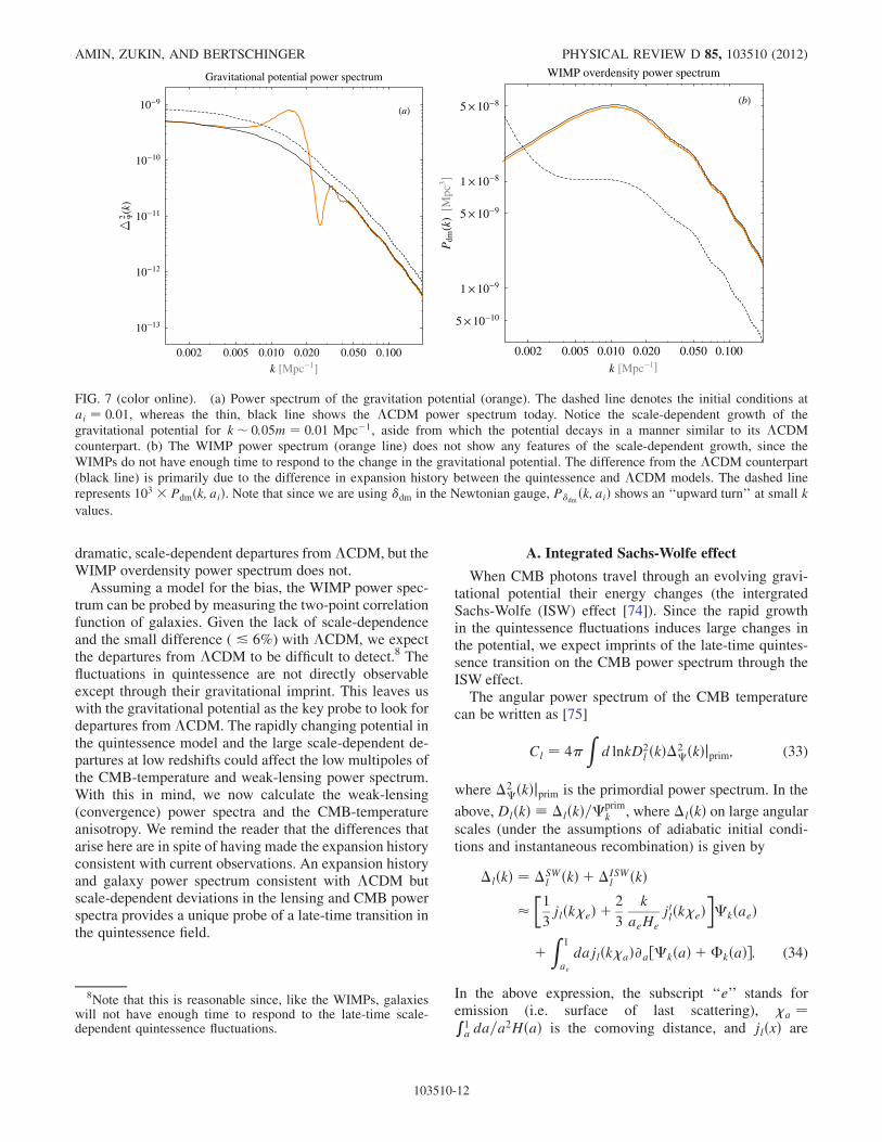
(with anl ¼ 0:95) are shown in Fig. 7 (thick, orange lines).The thin, black lines show the corresponding power spectrafor the�CDM cosmology. The gray, dashed lines show thepower spectra at ai ¼ 10�2. Note that since we are using�dm in the Newtonian gauge, P�dm
ðk; aiÞ shows an ‘‘upwardturn’’ at small k-values. By construction, the initial con-ditions in the power spectra ��ðk; aiÞ and Pdmðk; aiÞ in ourquintessence model and �CDM agree. The scale-dependent departures in ��ðk; aÞ arise after aosc � 0:8.As discussed previously, the enhancement can be trusteduntil anl ¼ 0:95, after which we freeze the potential untila ¼ 1. The wave number where the maximum departuresare seen is k� 0:05m � 0:01 Mpc�1. For k � H0 andk * m, the final spectrum closely resembles the �CDMcase. For fixed aosc, we have checked that the magnitude ofdeparture from�CDM increases with increasingm. This isconsistent with the notion larger m corresponds to a largermpl=M [see Eq. (10)], leading to more efficient resonance.
As discussed for single modes, the potential��ðk; aÞ show
SCALE-DEPENDENT GROWTH FROM A TRANSITION IN . . . PHYSICAL REVIEW D 85, 103510 (2012)
103510-11
dramatic, scale-dependent departures from�CDM, but theWIMP overdensity power spectrum does not.
Assuming a model for the bias, the WIMP power spec-trum can be probed by measuring the two-point correlationfunction of galaxies. Given the lack of scale-dependenceand the small difference ( & 6%) with �CDM, we expectthe departures from �CDM to be difficult to detect.8 Thefluctuations in quintessence are not directly observableexcept through their gravitational imprint. This leaves uswith the gravitational potential as the key probe to look fordepartures from �CDM. The rapidly changing potential inthe quintessence model and the large scale-dependent de-partures at low redshifts could affect the low multipoles ofthe CMB-temperature and weak-lensing power spectrum.With this in mind, we now calculate the weak-lensing(convergence) power spectra and the CMB-temperatureanisotropy. We remind the reader that the differences thatarise here are in spite of having made the expansion historyconsistent with current observations. An expansion historyand galaxy power spectrum consistent with �CDM butscale-dependent deviations in the lensing and CMB powerspectra provides a unique probe of a late-time transition inthe quintessence field.
A. Integrated Sachs-Wolfe effect
When CMB photons travel through an evolving gravi-tational potential their energy changes (the intergratedSachs-Wolfe (ISW) effect [74]). Since the rapid growthin the quintessence fluctuations induces large changes inthe potential, we expect imprints of the late-time quintes-sence transition on the CMB power spectrum through theISW effect.The angular power spectrum of the CMB temperature
can be written as [75]
Cl ¼ 4�Z
d lnkD2l ðkÞ�2
�ðkÞjprim; (33)
where �2�ðkÞjprim is the primordial power spectrum. In the
above, DlðkÞ � �lðkÞ=�primk , where �lðkÞ on large angular
scales (under the assumptions of adiabatic initial condi-tions and instantaneous recombination) is given by
�lðkÞ ¼ �SWl ðkÞ þ �ISW
l ðkÞ
��1
3jlðk�eÞ þ 2
3
k
aeHe
j0lðk�eÞ��kðaeÞ
þZ 1
ae
dajlðk�aÞ@a½�kðaÞ þ�kðaÞ�: (34)
In the above expression, the subscript ‘‘e’’ stands foremission (i.e. surface of last scattering), �a ¼R1a da=a
2HðaÞ is the comoving distance, and jlðxÞ are
a
0.002 0.005 0.010 0.020 0.050 0.100
10 13
10 12
10 11
10 10
10 9
k Mpc 1
Gravitational potential power spectrum
b
0.002 0.005 0.010 0.020 0.050 0.100
5 10 10
1 10 9
5 10 9
1 10 8
5 10 8
k Mpc 1
Pdm
kM
pc3
WIMP overdensity power spectrum
FIG. 7 (color online). (a) Power spectrum of the gravitation potential (orange). The dashed line denotes the initial conditions atai ¼ 0:01, whereas the thin, black line shows the �CDM power spectrum today. Notice the scale-dependent growth of thegravitational potential for k� 0:05m ¼ 0:01 Mpc�1, aside from which the potential decays in a manner similar to its �CDMcounterpart. (b) The WIMP power spectrum (orange line) does not show any features of the scale-dependent growth, since theWIMPs do not have enough time to respond to the change in the gravitational potential. The difference from the �CDM counterpart(black line) is primarily due to the difference in expansion history between the quintessence and �CDM models. The dashed linerepresents 103 � Pdmðk; aiÞ. Note that since we are using �dm in the Newtonian gauge, P�dm
ðk; aiÞ shows an ‘‘upward turn’’ at small k
values.
8Note that this is reasonable since, like the WIMPs, galaxieswill not have enough time to respond to the late-time scale-dependent quintessence fluctuations.
AMIN, ZUKIN, AND BERTSCHINGER PHYSICAL REVIEW D 85, 103510 (2012)
103510-12
spherical Bessel functions. The second term is the ISW-term, which gets large if the potential evolves significantlybetween last scattering and today. In �CDM the ISW-termgets a small contribution just after recombination since weare not quite matter-dominated at that time. But, the maincontribution on the scales of interest comes from late-timesas the Universe starts becoming �-dominated and thepotentials start decaying. The same effect is also presentin the quintessence model. However, there is an additionalcontribution from the late-time rapid growth of the poten-tial. This growth occurs in spurts [see Fig. 5(b)] and we canapproximate @a�k as a Dirac-delta function at the locationof the jumps in the gravitational potential. As a result, thecontribution of each jump to the ISW-term can be easilyevaluated
ðjÞ�ISWl ðkÞ � 2jlðk�ajÞ��kðajÞ; (35)
where aj is the scale factor where the potential jumps. For
a jump of order a few �k, the ‘‘jump’’ term is larger thanthe smooth ISW contribution in �CDM. Note that therecan be multiple jumps, both positive and negative depend-ing on the kmode in question. Also note that apart from themagnitude of the jump, the location aj also plays a role by
fixing the argument of the Bessel function.We expect that this growth affects the low multipole
moments of the CMB since the changes in the potentialoccur very recently. More specifically, the multipolerange where we expect deviations is l & k�aj , where k�0:05m � 0:01 Mpc�1. For the fiducial parameters chosenhere, this yields l & few. Note that along with k, it is thesmallness of�aj that limits the effect to large angular scales.
In order to quantitatively calculate the effect of thequintessence perturbations on the CMB power spectrum,we use the �kðaÞ and �kðaÞ evaluated from CMBFAST [68]for a < ai ¼ 0:01. This captures the contributions fromearly ISW as well as early anisotropic stress (which weignore at late times). For a > ai, we use �kðaÞ computedfrom our own independent code for �CDM and the quin-tessence model. As discussed before, for the quintessencecase we set @a�k ¼ 0 for a > anl. With this entire solutionat hand (for ae < a < 1), we compute the �lðkÞ and Cl.The ratio of the angular CMB power spectra for the quin-tessence and �CDM models is shown in Fig. 8(a). Notethat this is large enough to potentially rule out this choiceof parameters. Thus, we see that in spite of the effect beingon large angular scales, ISW provides an excellent probefor constraining the considered transition in quintessence.One can change parameters, for example aosc or m (equiv-alently M), to get the ISW effect small enough so that it isconsistent with observations. One has to first make surethat such changes are still consistent with the expansionhistory (see discussion in Sec. III). Increasing m or aosc orvarying m and aosc in opposite directions can lead to anexpansion history consistent with observations. Let us nowlook at perturbations. In general, for a fixed aosc, as weincrease m (equivalently decrease M), the fluctuationsgrow more rapidly, shifting the time when the potentialsgrow rapidly to smaller a values. One might expect thatthis will make the ISW contribution even larger. However,one finds that the effect on �lðkÞ is not quite as simple.First the change in growth of potential is quite sensitive tothe number of zero crossing of the homogeneous field. In
a
10.05.02.0 3.0 15.07.01
2
3
4
5
l
Cl
Cl
CD
M
Ratio of CMB angular power spectra
b
10.05.02.0 3.0 15.07.0
1.0
1.1
1.2
1.3
1.4
1.5
l
Cl
Cl
CD
M
Ratio of convergence power spectra
FIG. 8 (color online). (a) Ratio of CMB-temperature power spectrum at low multipoles between our quintessence and �CDMmodels. The large difference is due to the rapidly evolving gravitational potential in the quintessence model after aosc (b) Ratio of thelensing (convergence) power spectrum at low multipoles between our quintessence and �CDM models. The departures are restrictedto low l multipoles due to the proximity of the transition in the quintessence field responsible for the rapid growth in the gravitationalpotential. For lensing, the model does not agree with �CDM at large l due to the different expansion histories.
SCALE-DEPENDENT GROWTH FROM A TRANSITION IN . . . PHYSICAL REVIEW D 85, 103510 (2012)
103510-13
addition, changing parameters changes the wave numbers,which grow the fastest and the time when there is a rapidgrowth in the potential. Heuristically, this affects the argu-ment of the k� of the nonmonotonic-spherical Besselfunction in�lðkÞ. Similar considerations apply to changingaosc. As a result, it is somewhat difficult to apriori predictwhich combination of parameters (consistent with theobserved expansion history) will also yield an acceptableISW term. Indeed we find that m � 2� 103H0 and aosc �0:82 is entirely consistent with observations of the expan-sion history as well as the CMB. We also find regions ofparameter space with smaller values of m but larger valuesof aosc compared to the fiducial model consistent withobservations. A full sweep of parameters (including �) todetermine regions consistent with observations is beyondthe scope of this paper, but is certainly worth pursuing.
Before we move on to the calculation of the lensingpower spectrum, let us briefly comment on the additionalISW that can result from nonlinear field evolution after anl,ignored so far in the linearized treatment. As noted inSec. IVB3, the rapid growth of the linearized scalar-fieldperturbations is curtailed once the field perturbations be-come nonlinear (around anl). However, there will be furthernonlinear evolution and rapid fragmentation of the field. Toget an estimate of the resulting ISW effect, consider aspherical perturbation with massM and radius R, collaps-ing at speed v. Such a perturbation yields a temperaturedecrement of order�GMv=R. For a sphere with an initialradiusRnl � k�1
nl (with knl � 0:05m), an initial density com-
parable to the background energy density and v� 0:05 (theapproximate group velocity of a perturbation with wavenumber knl), the decrement can be �few� 10�5 for ourfiducial set of parameters (m� 103H0). The signal is quali-tatively similar to the Sunyaev-Zel’dovich temperature dec-rement from galaxy clusters [76]. However, unlike& arcmin angular scale of the SZ decrement, here, theangular scale is �30 degrees. This simple estimate showsthat it might be possible to get additional constraints on thequintessence transition from the ISWeffect due to the non-linear field evolution. Individual oscillons, modeled bydensity configurations with time-dependent radii �few�m�1 can also yield an additional ISW signal on smallerscales. We discuss a toy model for estimating the ISWsignal from such nonlinear perturbations in Appendix B.However, we again caution the reader that these numbersshould be checked with input from detailed simulations ofthe nonlinear field dynamics including gravity.
B. Weak lensing
Observational constraints from weak lensing observa-tions are often presented in terms of the weak lensingconvergence (angular) power spectrum [77,78]
Cl ¼ 8�2
Z �e
0d�W2ð�Þ l
��2
�ðk ¼ l��1; �Þ; (36)
where
Wð�Þ ¼Z �e
�d�0 �
0 � �
�0 �ð�0Þ; (37)
�2�ðk; �Þ is the power spectrum of the gravitational poten-
tial and �ð�Þ is the radial distribution of sources, normal-ized to
R�ð�Þd� ¼ 1. We use the source distribution
�ðzÞ / z2 exp½�ð1:41z=zmedÞ1:5� (38)
with zmed ¼ 1:26. This distribution approximates the gal-axy redshift distribution of the COSMOS survey [79]. Aswith the ISW effect, because of the closeness of the tran-sition to the present day, we expect the signal to be largestat lowmultipoles l & k�ðanlÞ � few. The proximity of thetransition also picks out sources at approximately 2�ðanlÞ.As a result as anl ! 1ð� ! 0Þ, we run out of sources to belensed. Thus in general, for a fixed enhancement of thegravitational potential, we expect the largest lensing signalto arise from the smallest anl still consistent with theexpansion history.The ratio between the weak lensing convergence power
spectrum for the quintessence model and �CDM is shownin Fig. 8(b). The errors associated with measuring theconvergence power spectrum is given by [77]:
f2; 30g. Hence this particular quintessence model cannot beconstrained using LSST measurements of the weak lensingpower spectrum. The weak lensing convergence powerspectrum for the quintessence model does not asymptoteto the �CDM prediction at higher l because there is adifference in expansion history between the two models.Even this deviation would be difficult to see using LSSTsince the minimum 4C
l =Cl � 0:1 at l� 300.
Before moving on to our conclusions, we note that thereare qualitative degeneracies between observational signa-tures (in particular, ISW at low multipoles) predicted byour scenario and those of other models, for example,interacting dark energy models with significant clustering(see [60,81–83]).
VI. CONCLUSIONS
For a slowly rolling quintessence field, it is natural(though not necessary) that the field will eventually startoscillating at it approaches a minimum in its potential. Inthis paper we have analyzed the consequences on the ex-pansion history and structure formation of a quintessence
AMIN, ZUKIN, AND BERTSCHINGER PHYSICAL REVIEW D 85, 103510 (2012)
103510-14
field, which initially behaves like dark energy and startsoscillating around the minimum in its potential at latetimes (a * 0:8). The potentials considered in detail herehave a quadratic minimum and are shallower than qua-dratic away from the minimum. When a spatially homoge-neous scalar field (’) oscillates about the minimum of suchan anharmonic potential, it can pump energy into its spa-tially inhomogeneous perturbations (�’) through paramet-ric resonance. The amount of energy transfer depends onboth the wave number of �’ as well as the number ofoscillations that take place in the background field. Thisleads to a rapid fragmentation of the homogeneous fieldand rapid resonant growth of the field fluctuations on timescales significantly shorter than H�1
0 .
In order to avoid discrepancies with the measured ex-pansion history and to simultaneously produce oscillationsin the field, we have given a prescription for setting theinitial conditions of the quintessence field and parametersin the potential. We have also explicitly shown that thepotentials must be close to constant during the phase wherethe field is slowly rolling. Potentials that do not satisfy thisrequirement have too much of a delay between the end ofslow-roll and the beginning of oscillations, thus avoidingthe rapid resonant growth of structure. Note that currentdata is consistent with a cosmological constant. Our modelis in no way more natural than a cosmological constantor other dark energy models. However, we believe thatthe model’s interesting phenomenology and potentiallyobservable consequences warrants its study.
Given a model that produces a background expansionhistory in good agreement with the measured expansionhistory, we have shown how the gravitational potential andthe overdensity in WIMPs is affected by the resonantgrowth of the field fluctuations. We found that the metricperturbations develop scale-dependent growth with the
scale set by the mass of the scalar-field potential m�ffiffiffiffiffiffiffiffiffiffiffiffiffiffiffiffiffiffiffiffiffiffiffiffiU00ð’ ! 0Þp � 103H0 (k & 0:1m). On the other hand,
the dark matter overdensity remains featureless and verysimilar to the �CDM solution aside from an overall slightsuppression because of the small difference in expansionhistory between �CDM and the quintessence model. Thisis because the dark matter does not have time to respond tothe changing potential. Note that scale-dependent changesin the gravitational potential are normally attributed tomodified gravity (e.g. [84–86]). Here, however, we haveshown that such a change can occur in general relativitywith a minimally coupled quintessence field with a canoni-cal kinetic term. Thus, if future observations find evidencefor scale-dependent growth, it cannot be attributed tomodified gravity.
The rapid growth of the potential significantly affects theISW contribution to the temperature angular power spec-trum of the CMB. For a range of parameters this yields thestrongest constraint on such quintessence transitions. Sincethe metric perturbation develops a scale-dependent change,
the weak lensing power spectrum also offers a possible wayto constrain this quintessence scenario, where dark energyundergoes a late-time transition described above.Unfortunately, because of the proximity of the decay indark energy, deviations from �CDM occur at low l multi-pole moments. A full treatment, which includes nonline-arities in the quintessence field, however, could give rise todeviations in the weak lensing and temperature powerspectrum at larger l values.The nonlinear dynamics of the quintessence field would
give rise to a wealth of new phenomenon including fieldfragmentation and possible formation of localized scalar-field lumps, which could provide additional observationalconstraints. The full nonlinear analysis, combing N-bodysimulations for the dark matter and lattice simulations forthe scalar field is beyond the scope of this paper, butprovides a promising avenue to explore quintessence tran-sitions and their consequences further. Recall that in spiteof its strong clustering properties, our quintessence field isminimally coupled with a canonical kinetic term and doesnot have nongravitational couplings to WIMP dark matter.This could make such models easier to simulate thanmodels where gravity is modified (e.g. [87–91]), interact-ing dark energy models (e.g. [83,92–94]), nonminimallycoupled quintessence (e.g. [95,96]) or when nonstandardkinetic terms are present.In summary, if dark energy changes its nature close
enough to the present time, it is possible to miss it in theexpansion history measurements. For the models consid-ered here, we have demonstrated that such a transition candramatically change the gravitational potential powerspectrum in a scale-dependent way but leave the galaxyclustering unaffected, thus providing a possibly uniquesignature of such a transition. The best constraints onsuch transitions likely come from the ISWeffect, followedby lensing. We expect a more involved analysis will pro-vide additional constraints on such a transition once weinclude: (i) the nonlinear collapse in WIMPs and in thequintessence field, which will increase power on smallerscales; (ii) couplings to other fields (ignored here). Itwould also be interesting to explore similar resonantgrowth in models with multiple ultralight scalar fields(not necessarily dark energy) motivated in [97] andstudied in more detail in the context of structure forma-tion by [98].
ACKNOWLEDGMENTS
We would like to thank Alan Guth, David Shirokoff,Raphael Flauger, Richard Easther, Andrew Liddle, VolkerSpringel, Robert Crittenden, Marco Bruni, Ignacy Sawicki,Jonathan Pritchard, Navin Sivanandam and CharlesShapiro for useful conversations. We would especiallylike to thank Mark Hertzberg for comments on an earlydraft of this work and Antony Lewis for repeated andprompt help when we were trying to check our ISW
SCALE-DEPENDENT GROWTH FROM A TRANSITION IN . . . PHYSICAL REVIEW D 85, 103510 (2012)
103510-15
calculation using CAMB.We thank the anonymous refereefor a number of constructive comments.
The linearized equations of motion for the fluctuations,neglecting the Hubble expansion and metric perturbation,are (in Fourier space)
@2t �’k þ ½k2 þU00ð �’Þ��’k ¼ 0; (A1)
where k is the wave number. Since the homogeneous field’ is oscillating, U00ð’Þ is periodic in time. This results in alinear system with periodic coefficients can be analyzedwith Floquet theory. Floquet’s theorem is most elegantlywritten in matrix form. Converting our second-order equa-tion of motion into a first-order matrix equation, we find
@txðtÞ ¼ EðtÞxðtÞ; (A2)
where
xðtÞ ¼ �’k
@t�’k
� �and
EðtÞ ¼ 0 1�k2 �U00ð �’Þ 0
� �:
Before stating Floquet’s theorem, we need one moredefinition. The fundamental matrix solution Oðt; t0Þ, ofEq. (A2) satisfies
@tOðt; t0Þ ¼ EðtÞOðt; t0Þ; Oðt0; t0Þ ¼ 1: (A3)
The fundamental matrix solution evolves the initial con-ditions xðt0Þ in time
xðtÞ ¼ Oðt; t0Þxðt0Þ: (A4)
Explicitly, Oðt; t0Þ consists of two columns that representtwo independent solutions x1, x2, which satisfy x1ðt0Þ ¼ð1; 0Þ and x2ðt0Þ ¼ ð0; 1Þ. Note that det Oðt; t0Þ is theWronskian, det Oðt0; t0Þ ¼ 1, and there are no ‘‘friction’’terms. Hence by Abel’s Identity we have det Oðt; t0Þ ¼ 1.
We are now ready to state Floquet’s theorem (withoutproof). Consider the linear system
@txðtÞ ¼ EðtÞxðtÞ; (A5)
where x is a column vector and E is a real 2� 2 matrixsatisfying Eðtþ TÞ ¼ EðtÞ for all t. The fundamental so-lution Oðt; t0Þ is
O ðt; t0Þ ¼ Pðt; t0Þ exp½ðt� t0ÞMðt0Þ�; (A6)
where Pðtþ T; t0Þ ¼ Pðt; t0Þ and Mðt0Þ satisfies Oðt0 þT; t0Þ ¼ exp½TMðt0Þ�. The eigenvalues �1;2 of Mðt0Þ arecalled Floquet exponents.
Since det Oðt0 þ T; t0Þ ¼ 1, we have �1 þ�2 ¼ 0.Suppose, from now on, that �1 ¼ ��2 ¼ �. If Mðt0Þ
has two linearly independent eigenvectors e�ðt0Þ corre-sponding to �� (including � ¼ 0), then the general solu-tion can be written as
where P�ðt; t0Þ ¼ Pðt; t0Þe�ðt0Þ are periodic column vec-tors. If there exists only one eigenvector corresponding tothe repeated eigenvalue � ¼ 0, then the general solutionbecomes
where P gðt; t0Þ ¼ Pðt; t0Þegðt0Þwith egðt0Þ is a generalizedeigenvector.From above discussion, we have exponentially growing
solutions if the real part of the Floquet exponents <½�� �0. In order to calculate Floquet exponents ��, it is usefulto consider the eigenvalues �� of Oðt0 þ T; t0Þ calledFloquet multipliers. Since detOðt0 þ T; t0Þ ¼ 1, then�þ ��� ¼ 1. They are related to the Floquet exponents via�� ¼ e�T�. In general � and �� are complex. Using�� ¼ j��jei�� and �þ � �� ¼ 1, we have
� ¼ 1
T½lnj�þj þ i�þ� ¼ � 1
T½lnj��j þ i���:
Thus, <½�� � 0 if j��j � 1.Calculating the Floquet exponents explicitly for the
problem at hand reduces to the following steps:(1) First we calculate the period T of U. The period of
UðtÞ depends on the initial amplitude of the homo-geneous field �’ðt0Þ (assuming @t �’ðt0Þ ¼ 0) and isgiven by
Tð �’maxÞ ¼ 2Z �’max
�’min
d �’ffiffiffiffiffiffiffiffiffiffiffiffiffiffiffiffiffiffiffiffiffiffiffiffiffiffiffiffiffiffiffiffiffiffiffiffiffiffiffi2Vð �’maxÞ � 2Vð �’Þp : (A9)
In practice, we specify either �’max or �’min. Theother is found by solving Vð �’minÞ ¼ Vð �’maxÞ. ForVð’Þ ¼ Vð�’Þ we have �’max ¼ �’min.
(2) Next we solve @tOðt; t0Þ ¼ EðtÞOðt; t0Þ from t0 tot0 þ T to obtain
Oðt; t0Þ ¼�’ð1Þ
k ðt0 þ TÞ �’ð2Þk ðt0 þ TÞ
@t�’ð1Þk ðt0 þ TÞ @t�’
ð2Þk ðt0 þ TÞ
0@
1A;
where f�’ð1Þk ðt0Þ¼1;@t�’
ð1Þk ðt0Þ¼0g and f�’ð2Þ
k ðt0Þ¼0;@t�’
ð2Þk ðt0Þ¼1g. This is equivalent to solving
@2t ’k þ ½k2 þ V 00ð �’Þ��’k ¼ 0 for the above twosets of initial conditions from t0 to t0 þ T. We havesuppressed the dependence of T on �’max to reduceclutter.
(3) Last, we find the eigenvalues of Oðt0 þ T; t0Þ. Theyare
AMIN, ZUKIN, AND BERTSCHINGER PHYSICAL REVIEW D 85, 103510 (2012)
where all quantities are evaluated at t0 þ T. Notethat since the �’kðt0 þ TÞ depends on k, the eigen-values also depend on k. The Floquet exponents��are then given by
APPENDIX B: ISW EFFECT FROM NONLINEARDYNAMICS OF THE QUINTESSENCE FIELD
In the main body of the text, we discussed how thequintessence field fluctuations grow rapidly during theoscillatory regime. This rapid growth leads to a scale-dependent growth in the gravitational potential which inturn leads to large changes in the CMB-temperature an-isotropies via the integrated Sachs-Wolfe effect (seeSec. VA). However, after anl � 0:95 the field perturbationsbecome nonlinear and the homogeneous field fragmentsrapidly, potentially forming long-lived, localized excita-tions of the field called oscillons. Our linear analysis didnot include the ISW effect resulting from the nonlinearevolution of the field perturbations. In this Appendix, weremedy this by estimating the change in the CMB-temperature due to the following:
(i) The change in the gravitational potential from theinitial quasi/nonlinear evolution of the fieldperturbations.
(ii) The time varying gravitational potential due to anisolated oscillon after it is formed.
Let us first look at the ISWeffect from the initial evolutionof quasi/nonlinear perturbations. A realistic calculationrequires input from detailed simulations of the nonlinearfield dynamics (for example, [15]). Here we concentrate ona related toy problem of calculating the ISW effect due tothe collapse of a single, spherical top-hat overdensity. Thisrepresents a crude approximation to the initial rapid quasi/nonlinear evolution of density perturbations associatedwith our model of quintessence. Later, we will evaluatethe CMB-temperature anisotropies from the ISWeffect dueto a stable oscillonlike configuration. Since the Universeexpands very little between anl � 0:95 and a ¼ 1, we willwork in a Minkowski background. Our main purpose is to
obtain an order of magnitude estimate and understand howthe effect depends on aspects of nonlinear evolution.Consider a spherical mass M with uniform density
and a time-dependent radius RðtÞ located at xc. The gravi-tational potential due to this mass is given by
�ðt;xÞ ¼8><>:� GM
jx�xcj jx� xcj> RðtÞ;GM2R
�jx�xcj2
R2 � 3
�jx� xcj RðtÞ:
The partial-time derivative of this potential is
@t�ðt;xÞ ¼ 3GM _R
2R4u�ðuÞ; (B1)
where u ¼ R2ðtÞ � jx� xcj2 and� is the Heaviside func-tion. The change in the CMB temperature due to a time-varying potential (ISW term) is
�TðnÞT
¼ 2Z t0
tnl
dt@t�ðt;xÞjx¼ðt0�tÞn; (B2)
where n is a unit vector that defines observer’s line of sight,t0 is the time since last scattering � 0:99H�1
0 , and we
replace x by ðt0 � tÞn since light travels on null geodesics.We have ignored anisotropic stress here (� ¼ �). Notethat the time of integration starts at tnl � 0:94H�1
0 (corre-
sponding to anl � 0:95) since nonlinear perturbations donot exist beforehand.Let us consider ‘‘linear’’ collapse, i.e.
and xc. Note that t� and tþ denote the time a light rayenters and exist the spherical mass. With these definitionsat hand, the integral over time in Eq. (B2) can be evaluatedanalytically. In particular, if tnl < t� < tþ < t0 (and Rc >0) we find
�TðnÞT
¼ � 4GMvð1� v2Þ2r3cðR2
c � vr2cÞ2: (B5)
Recalling that rc and Rc depend on the angle �, the aboveexpression shows that we should expect a cold-spot in theCMB, with an angular size �Rc=jxcj. The anisotropy isnegative and maximal when � ¼ 0; when the light raypasses through the center of the mass distribution
�TðnÞT
��������max¼ � 4GMv
Rc
: (B6)
The result depends only on the size of the sphere Rc whenthe light passes through its center, the speed of collapse vand the massM. To obtain an order of magnitude estimate,we use our fiducial set of parameters. We choose an initial
SCALE-DEPENDENT GROWTH FROM A TRANSITION IN . . . PHYSICAL REVIEW D 85, 103510 (2012)
103510-17
perturbation of size Rnl � k�1nl � ð0:05mÞ�1 � 0:02H�1
0
see Sec. IVB2 and IVB3), with density of order the criticaldensity. We put the perturbation a distancejxcj ¼ 0:03H�1
0
from us (corresponding �ðt0 � tnlÞ=2) and impose that itcollapses with v� 0:05 (the approximate group velocity ofa perturbation with wave number knl). We get
�TðnÞT
��������max�� 4� 10�5; (B7)
which could provide additional constraints on our models.This signal is qualitatively similar to the Sunyaev-Zel’dovich temperature decrement from galaxy clusters[76]. However unlike & arcmin angular scale of the SZdecrement, here the angular scale is �30 degrees. As canbe checked, the conditions tnl < t� < tþ < t0 and Rc > 0are satisfied for the above-mentioned parameters. We re-mind the reader that this is merely an estimate based on aspherical top-hat collapse. The actual nonlinear field evolu-tion can be more complicated. In addition, the amplitude ofthe effect depends on the parameters in a nontrivial manner.Nevertheless, this exercise shows that it is indeed interestingto pursue the nonlinear evolution of the scalar-field pertur-bations in detail.
Let us now consider the ISW effect resulting from thetime-varying potential associated with a single oscillon.Based on our numerical solutions (radial only), oscillonswith a central field amplitude of order M9 and width oforder few m�1 have a peak energy density of order m2M2
and an energy density profile that breathes in and out. Thisis in contrast with a fixed-energy density profile often usedin the oscillon literature. For an oscillon, crudely approxi-mated by the a top-hat density configuration, we take
RoscðtÞ � 2m�1
�1þ 1
4sin2½mtþ��
�; (B8)
where for our fiducial modelm� 103H0. We stress that theactual energy density profile of oscillons in our model ismore complicated. The energy density profile resembles aGaussian when the central-field amplitude is at its maxi-mum, but becomes flatter when the field amplitude passes
through zero. As a result, a calculation based on realisticoscillon profiles could be somewhat different from theestimates below.Unlike the linear collapse case, we did not find a simple
analytic expression for the ISW contribution from individ-ual oscillons. Evaluating it numerically, we find that for ourfiducial set of parameters and assuming that the energydensity within oscillons ��m2M2 � 3H2
0m2pl, we get
�TðnÞT
��������max��GMoscm� 10�2 ��10�7: (B9)
We have assumed that the oscillon is located at jxcj �0:03H�1
0 . The shape of the anisotropy pattern is ringlike.
The phase of the radial oscillation � determines whetherthe center has a temperature decrement or increment. Notethat the radius associated with an individual oscillon issmall compared to the quasilinear perturbations consideredearlier in this Appendix (by an order of magnitude). As aresult, one expects a smaller effect if one assumes that theirdensity is still comparable to the average cosmologicaldensity. In addition, since the light crossing time is com-parable to the oscillatory time scale of the energy densityconfiguration, the ISW-term undergoes cancellations, lead-ing to a somewhat smaller ISW effect than what would beexpected on purely dimensional grounds. Thus we expectthe ISW contribution from individual oscillons to besmaller (and more localized) than that from the rapidcollapse of nonlinear perturbations.Before we end this Appendix, we would like to comment
on a caveat regarding the emergence of oscillons. Our linearanalysis in the main body of the paper revealed that pertur-bations become nonlinear at anl. While the nonlinear per-turbations will form oscillons eventually, it is worth askingwhether we can see them as large overdensities with indi-vidual identities by today. To unambiguously understandthe time scales associated with emergence of oscillonswould require a full lattice simulation, which is beyondthe scope of this current paper. Our analysis here indicatesthat it is certainly worth exploring this further. While here,we have concentrated on isolated inhomogeneities, it wouldbe interesting to look at the combined effect of a collectionof such inhomogeneities (with a number density of orderðknl=2�Þ3) [9], which would be closer to the actualscenario.
[1] A. H. Guth, Phys. Rev. D 23, 347 (1981).[2] A. D. Linde, Phys. Lett. B 108, 389 (1982).[3] A. Albrecht and P. J. Steinhardt, Phys. Rev. Lett. 48, 1220
(1982).[4] B. Ratra and P. J. E. Peebles, Phys. Rev. D 37, 3406
(1988).
[5] C. Armendariz-Picon, V. F. Mukhanov, and P. J.
Steinhardt, Phys. Rev. Lett. 85, 4438 (2000).[6] E. J. Copeland, M. Sami, and S. Tsujikawa, Int. J. Mod.
Phys. D 15, 1753 (2006).[7] J. H. Traschen and R.H. Brandenberger, Phys. Rev. D 42,
2491 (1990).
9This M determines the scale where the scalar-field potentialchanges shape, and should not be confused with M use todenote the mass of perturbations.
AMIN, ZUKIN, AND BERTSCHINGER PHYSICAL REVIEW D 85, 103510 (2012)
[8] L. Kofman, A. D. Linde, and A.A. Starobinsky, Phys. Rev.Lett. 73, 3195 (1994).
[9] M.A. Amin, Phys. Rev. DarXiv:1006.3075v2.[10] M.A. Amin, R. Easther, and H. Finkel, J. Cosmol.
Astropart. Phys. 12 (2010) 001.[11] R. Allahverdi, R. Brandenberger, F. Y. Cyr-Racine, and A.
Mazumdar, Annu. Rev. Nucl. Part. Sci. 60, 27 (2010).[12] J. A. Frieman, C. T. Hill, A. Stebbins, and I. Waga, Phys.
Rev. Lett. 75, 2077 (1995).[13] M. Khlopov, B.A. Malomed, and I. B. Zeldovich, Mon.
Not. R. Astron. Soc. 215, 575 (1985).[14] M.C. Johnson and M. Kamionkowski, Phys. Rev. D 78,
063010 (2008).[15] M.A. Amin, R. Easther, H. Finkel, R. Flauger, and M. P.
Hertzberg, arXiv:1106.3335v2.[16] I. L. Bogolyubsky and V.G. Makhankov, Pis’ma Zh. Eksp.
Teor. Fiz. 24, 15 (1976).[17] H. Segur and M.D. Kruskal, Phys. Rev. Lett. 58, 747
(1987).[18] M. Gleiser, Phys. Rev. D 49, 2978 (1994).[19] E. J. Copeland, M. Gleiser, and H. R. Muller, Phys. Rev. D
52, 1920 (1995).[20] J. McDonald, Phys. Rev. D 66, 043525 (2002).[21] S. Kasuya, M. Kawasaki, and F. Takahashi, Phys. Lett. B
559, 99 (2003).[22] M. Gleiser and R. C. Howell, Phys. Rev. Lett. 94, 151601
(2005).[23] M. Gleiser, Int. J. Mod. Phys. D 16, 219 (2007).[24] M. Hindmarsh and P. Salmi, Phys. Rev. D 74, 105005
(2006).[25] P.M. Saffin and A. Tranberg, J. High Energy Phys. 01
(2007) 030.[26] E. Farhi, N. Graham, A.H. Guth, N. Iqbal, R. R. Rosales,
and N. Stamatopoulos, Phys. Rev. D 77, 085019 (2008).[27] G. Fodor, P. Forgacs, Z. Horvath, and M. Mezei, Phys.
Lett. B 674, 319 (2009).[28] M. Gleiser and D. Sicilia, Phys. Rev. D 80, 125037 (2009).[29] M.A. Amin and D. Shirokoff, Phys. Rev. D 81, 085045
(2010).[30] M. P. Hertzberg, Phys. Rev. D 82, 045022 (2010).[31] M. Gleiser, N. Graham, and N. Stamatopoulos, Phys. Rev.
D 82, 043517 (2010).[32] M. Gleiser, N. Graham, and N. Stamatopoulos, Phys. Rev.
D 83, 096010 (2011).[33] S. Y. Khlebnikov and I. I. Tkachev, Phys. Rev. D 56, 653
(1997).[34] R. Easther and E.A. Lim, J. Cosmol. Astropart. Phys. 04
(2006) 010.[35] J. F. Dufaux, A. Bergman, G.N. Felder, L. Kofman, and
J. P. Uzan, Phys. Rev. D 76, 123517 (2007).[36] M.Y. Khlopov, Res. Astron. Astrophys. 10, 495
(2010).[37] S. DeDeo, R. R. Caldwell, and P. J. Steinhardt, Phys. Rev.
D 67, 103509 (2003).[38] J. Weller and A.M. Lewis, Mon. Not. R. Astron. Soc. 346,
987 (2003).[39] R. Bean and O. Dore, Phys. Rev. D 69, 083503
(2004).[40] W. Hu and R. Scranton, Phys. Rev. D 70, 123002 (2004).[41] D. Rapetti, S.W. Allen, and J. Weller, Mon. Not. R.
Astron. Soc. 360, 555 (2005).
[42] J.-M. Alimi, A. Fuzfa, V. Boucher, Y. Rasera, J. Courtin,and P.-S. Corasaniti, Mon. Not. R. Astron. Soc. 401, 775(2010).
[43] R. de Putter, D. Huterer, and E.V. Linder, Phys. Rev. D 81,103513 (2010).
[44] R. Bean, E. E. Flanagan, and M. Trodden, Phys. Rev. D 78,023009 (2008).
[45] D. Bertacca, M. Bruni, O. F. Piattella, and D. Pietrobon, J.Cosmol. Astropart. Phys. 02 (2011) 018.
[46] M. Mortonson, W. Hu, and D. Huterer, Phys. Rev. D 80,067301 (2009).
[47] E. Silverstein and A. Westphal, Phys. Rev. D 78, 106003(2008).
[48] L. McAllister, E. Silverstein, and A. Westphal, Phys. Rev.D 82, 046003 (2010).
[49] R. Flauger, L. McAllister, E. Pajer, A. Westphal, and G.Xu, J. Cosmol. Astropart. Phys. 06 (2010) 009.
[50] R. Kallosh and A. Linde, J. Cosmol. Astropart. Phys. 11(2010) 011.
[51] X. Dong, B. Horn, E. Silverstein, and A. Westphal, Phys.Rev. D 84, 026011 (2011).
[52] S. Panda, Y. Sumitomo, and S. P. Trivedi, Phys. Rev. D 83,083506 (2011).
[53] L. J. Hall, Y. Nomura, and S. J. Oliver, Phys. Rev. Lett. 95,141302 (2005).
[54] P. Serra, A. Cooray, D. E. Holz, A. Melchiorri, S. Pandolfi,and D. Sarkar, Phys. Rev. D 80, 121302 (2009).
[55] C. Blake et al., arXiv:1108.2637.[56] E. V. Linder, Astropart. Phys. 25, 167 (2006).[57] S. Dutta and R. J. Scherrer, Phys. Rev. D 78, 083512
(2008).[58] R. Lazkoz, V. Salzano, and I. Sendra, Phys. Lett. B 694,
198 (2010).[59] S. Dutta and I. Maor, Phys. Rev. D 75, 063507 (2007).[60] L. Amendola, M. Baldi, and C. Wetterich, Phys. Rev. D
78, 023015 (2008).[61] E. R.M. Tarrant, C. van de Bruck, E. J. Copeland, and
A.M. Green, Phys. Rev. D 85, 023503 (2012).[62] M. Baldi, Mon. Not. R. Astron. Soc. 420, 430 (2012)[63] E. Komatsu et al. (MAP Collaboration), Astrophys. J.
Suppl. Ser. 192, 18 (2011).[64] D. Rapetti, S.W. Allen, M.A. Amin, and R.D. Blandford,
Mon. Not. R. Astron. Soc. 375, 1510 (2007).[65] T.M. Davis, E. Mortsell, J. Sollerman, A. C. Becker, S.
Blondin, P. Challis, A. Clocchiatti, A. V. Filippenko, R. J.Foley, and P.M. Garnavichet al., Astrophys. J. 666, 716(2007).
[66] A. G. Riess, L. Macri, S. Casertano, M. Sosey, H.Lampeitl, H. C. Ferguson, A. V. Filippenko, S.W. Jha,W. Li, R. Chornock, and D. Sarkar, Astrophys. J. 699,539 (2009).
[67] R. Kessler et al., Astrophys. J. Suppl. Ser. 185, 32(2009).
[68] U. Seljak and M. Zaldarriaga, Astrophys. J. 469, 437(1996).
[69] S. Weinberg, Cosmology (Oxford University Press,Oxford, 2008).
[70] W. Magnus and S. Winkler, Hills Equation (IntersciencePublishers, New York, 1966)
[71] L. Kofman, A. D. Linde, and A.A. Starobinsky, Phys. Rev.D 56, 3258 (1997).
SCALE-DEPENDENT GROWTH FROM A TRANSITION IN . . . PHYSICAL REVIEW D 85, 103510 (2012)
[72] G. Fodor, P. Forgacs, Z. Horvath, and M. Mezei, Phys.Rev. D 79, 065002 (2009).
[73] M. Gleiser and D. Sicilia, Phys. Rev. Lett. 101, 011602(2008).
[74] R. K. Sachs and A.M. Wolfe, Astrophys. J. 147, 73(1967).
[75] C.-P. Ma and E. Bertschinger, Astrophys. J. 455, 7 (1995).[76] T.A. Marriageet al., Astrophys. J. 737, 61 (2011).[77] N. Kaiser, Astrophys. J. 498, 26 (1998).[78] W. Hu, Astrophys. J. 522, L21 (1999).[79] R. Massey, J. Rhodes, A. Leauthaud, P. Capak, R. Ellis, A.
Koekemoer, A. Refregier, N. Scoville, J. E. Taylor, J.Albert, J. Berge, C. Heymans, D. Johnston, J.-P. Kneib,Y. Mellier, B. Mobasher, E. Semboloni, P. Shopbell, L.Tasca, and L. Van Waerbeke, Astrophys. J. Suppl. Ser.172, 239 (2007).
[80] Z. Ivezic, et al., (LSST Collaboration),arXiv:0805.2366v2.
[81] V. Pettorino, N. Wintergerst, L. Amendola, and C.Wetterich, Phys. Rev. D 82, 123001 (2010).
[82] M. Baldi, V. Pettorino, L. Amendola, and C. Wetterich,Mon. Not. R. Astron. Soc. 418, 214 (2011).
[83] M. Baldi, in ‘‘Proceedings Volume of the Conference:Advances in Computational Astrophysics’’ (AstronomicalSociety of the Pacific, Cefalu, Italy, 2011).
[84] M.A. Amin, R. V. Wagoner, and R.D. Blandford, Mon.Not. R. Astron. Soc. 390, 131 (2008).
[85] E. Bertschinger and P. Zukin, Phys. Rev. D 78, 024015(2008).
[86] B. Jain and J. Khoury, Ann. Phys. (N.Y.) 325, 1479 (2010).[87] I. Laszlo and R. Bean, Phys. Rev. D 77, 024048 (2008).[88] F. Schmidt and F. Schmidt, Phys. Rev. D 80, 043001
(2009).[89] Y. Li and W. Hu, Phys. Rev. D 84, 084033 (2011).[90] S. Ferraro, F. Schmidt, and W. Hu, Phys. Rev. D 83,
063503 (2011).[91] G.-B. Zhao, B. Li, and K. Koyama, Phys. Rev. Lett. 107,
071303 (2011).[92] M. Baldi, V. Pettorino, G. Robbers, and V. Springel, Mon.
Not. R. Astron. Soc. 403, 1684 (2010).[93] B. Li, J. D. Barrow, Mon. Not. R. Astron. Soc. 413, 262–
270 (2011).[94] M. Baldi, Mon. Not. R. Astron. Soc. 411, 1077 (2011).[95] M.A. Rodriguez-Meza, AIP Conference Proceedings
1116, 171 (2009).[96] B. Li, D. F. Mota, and J. D. Barrow, Astrophys. J. 728, 109
(2011).[97] A. Arvanitaki, S. Dimopoulos, S. Dubovsky, N. Kaloper,
and J. March-Russell, Phys. Rev. D 81, 123530 (2010).[98] D. J. E. Marsh and P.G. Ferreira, Phys. Rev. D 82, 103528
(2010).
AMIN, ZUKIN, AND BERTSCHINGER PHYSICAL REVIEW D 85, 103510 (2012)