Scale-free Fluctuations in Bose-Einstein Condensates ...

Scale-free Fluctuationsin Bose-Einstein Condensates,

Quantum Dots and Music Rhythms

Dissertation

zur Erlangung des Doktorgrades

der Mathematisch-Naturwissenschaftlichen Fakultäten

der Georg-August-Universität zu Göttingen

vorgelegt von

Holger Hennig

aus Hamburg

Göttingen 2009

D7

Referent : Prof. Dr. Theo Geisel

Korreferent : Prof. Dr. Kurt Schönhammer

Tag der mündlichen Prüfung : 27.05.2009

Abstract

Mesoscopic systems are prone to substantial fluctuations that typically can notbe neglected or avoided. The understanding of the origin and the consequencesof these fluctuations (e.g. for transport measurements) is thus a fundamental partof the theory of mesoscopic systems. We will encounter scale-free fluctuations indifferent kinds of complex nonlinear systems in this thesis, which consists of twomain parts. The first part deals with Bose-Einstein condensates (BECs) in leakingoptical lattices. Experimentalists have achieved an extraordinary level of controlover BECs in optical traps in the past decade, which allows for the investigationof complex solid state phenomena and the emerging field of ’atomtronics’ promisesa new generation of nanoscale devices. It is therefore both of fundamental andtechnological importance to understand the dynamics and transport properties ofBECs in optical lattices. We study the outgoing atomic flux of BECs loaded in aone dimensional optical lattice with leaking edges, using a mean field descriptionprovided by the discrete nonlinear Schrödinger equation with nonlinearity Λ. Wefind that for a nonlinearity larger than a threshold Λ>Λb the dynamics evolves intoa population of discrete breathers, preventing the atoms from reaching the leakingboundaries. We show that collisions of other lattice excitations with the outermostdiscrete breathers result in avalanches, i.e. jumps of size J in the outgoing atomicflux, which follow a scale-free distribution P(J) ∼ 1/Jα characterizing systems ata phase transition. Our results are also relevant in a variety of other contexts,e.g. coupled nonlinear optical waveguides.

In the second part, fractal fluctuations in two different complex systems arestudied. Firstly, conductance fluctuations in mesoscopic systems (such as quan-tum dots) are considered, which are a sensitive probe of electron dynamics andchaotic phenomena. Using the standard map as a paradigmatic model, we showthat classical transport through chaotic Hamiltonian systems in general producesfractal conductance curves. This might explain unexpected results of experimentsin semiconductor quantum dots where a dependence of the fractal dimension onthe coherence length was observed. Furthermore, we predict fractal fluctuationsin the conductance of low-dimensional Hamiltonian systems with purely chaoticphase space.

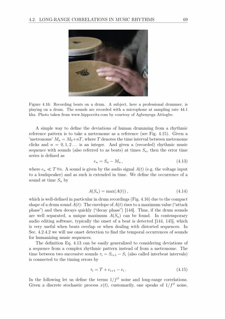
Secondly, we investigate temporal (fractal) fluctuations of human music rhythmscompared with an exact pattern, e.g. given by a metronome. We show that thetemporal fluctuations in simple as well as in more complex music rhythms aregeneric in the sense, that Gaussian 1/fβ noise is produced, no matter whetherthe rhythmic task is accomplished with hands, feet, the voice or a combination ofthese. Professional audio editing software includes a so-called ’humanizing’ feature,which adds deviations ξn to a given audio sequence, where ξn is white noise. Wedemonstrate that 1/f humanized music that we created is rated significantly betterby listeners than conventionally humanized sequences.

Kurzfassung

Mesoskopische Systeme unterliegen substanziellen Fluktuationen, die typischer-weise nicht vernachlässigt oder vermieden werden können. Das Verständnis des Ur-sprungs und der Folgen dieser Fluktuationen (z.B. für Transportmessungen) istdaher ein fundamentaler Teil der Theorie mesoskopischer Systeme. In dieser Ar-beit, welche aus zwei Teilen besteht, werden uns skalenfreie Fluktuationen in ver-schiedenen komplexen nichtlinearen Systemen begegnen. Der erste Teil handelt vonBose-Einstein Kondensaten (BECs) in undichten optischen Gittern. Experimenta-toren haben in der letzten Dekade einen außerordentlichen Grad an Kontrolle überBECs in optischen Fallen erreicht, was die Untersuchung von komplexen Festkör-perphänomenen ermöglicht und das aufkommende Feld ’Atomtronics’ versprichteine neue Generation von Nanobausteinen. Es ist daher sowohl von fundamentalerals auch von technologischer Bedeutung die Dynamik und die Transporteigenschaf-ten von BECs in optischen Gittern zu verstehen. Wir untersuchen den Fluss vonAtomen eines BECs aus einem eindimensionalen optischen Gitter mit undichtemRand und benutzen eine Molekularfeld-Näherung gegeben durch die diskrete nicht-lineare Schrödingergleichung mit Nichtlinearität Λ. Wir beobachten, dass bei einerNichtlinearität größer als ein Schwellenwert Λ > Λb die Dynamik zur Entstehungvon diskreten Solitonen führt, welche die Atome davon abhalten, den undichtenRand zu erreichen. Wir zeigen, dass Kollisionen von anderen Gitteranregungen mitden äußersten diskreten Solitonen zu Lawinen führen, d.h. Sprünge der Größe J indem Fluss von Atomen, die einer skalenfreien Verteilung P(J) ∼ 1/Jα folgen, wasSysteme an einem Phasenübergang charakterisiert. Unsere Ergebnisse sind auchrelevant in diversen anderen Kontexten, z.B. gekoppelte nichtlineare optische Wel-lenleiter.

Im zweiten Teil befassen wir uns mit fraktalen Fluktuationen in zwei verschie-denen komplexen Systemen. Zunächst werden Leitwertfluktuationen in mesosko-pischen Systemen (wie zum Beispiel Quantenpunkte) betrachtet, die eine sensibleSonde für die Dynamik von Elektronen und chaotische Phänomene sind. Mittelsder Standardabbildung als paradigmatisches Modell der Dynamik im gemischtenPhasenraum wird gezeigt, dass der klassische Transport durch Hamiltonsche Syste-me ganz allgemein fraktale Leitwertkurven hervorbringt. Dies könnte unerwarteteErgebnisse von Experimenten mit Halbleiter-Quantenpunkten erklären, bei deneneine Abhängigkeit der fraktalen Dimension von der Kohärenzlänge beobachtet wur-de. Darüber hinaus sagen wir fraktale Fluktuationen in dem Leitwert niedrigdimen-sionaler Hamiltonscher Systeme mit rein chaotischem Phasenraum vorher.

Zweitens betrachten wir zeitliche (fraktale) Fluktuationen von menschlichenMusikrhythmen verglichen mit einem exakten Muster, z.B. gegeben durch ein Me-tronom. Es wird gezeigt, dass zeitliche Fluktuationen in einfachen und in komplexe-ren Musikrhythmen generisch sind, in dem Sinne, dass Gaußsches 1/fβ Rauschenproduziert wird, ganz gleich ob eine rhythmische Aufgabe mit Händen, Füßen,der Stimme oder einer Kombination dieser ausgeführt wird. Professionelle Audio-Bearbeitungssoftware beinhaltet ein sogenanntes ’Humanizing’-Werkzeug, welchesAbweichungen ξn zu einer gegebenen Audiosequenz hinzufügt, wobei ξn weissesRauschen ist. Wir zeigen, dass von uns kreierte 1/f -humanisierte Musik signifikantbesser von Zuhörern bewertet wird als konventionell humanisierte Sequenzen.

Acknowledgments

First, it is a pleasure for me to thank my advisor, Theo Geisel, for the possibility towork in his unique group, for illuminating discussions, and for constant support ofmy plans. With his continuous effort he creates excellent working conditions anda great atmosphere in the institute.

Special thanks are due to Ragnar Fleischmann, for supporting me in so many waysthroughout the years, for teaching me nonlinear dynamics, inspiring discussions,for giving me the freedom to pursue a variety of different projects and own ideas,and for his kind-heartedness and humor.

I would like to thank Tsampikos Kottos for the fruitful collaboration on BECs, Ilearned a lot during our active video conferences that included plenty of questionsand ideas. Also, it was a pleasure to collaborate with Gim Seng Ng, thank you aswell for being a delightful office mate during your visits in Göttingen in summers.

I had the opportunity to stay at Boston University from May-September 2008 andto learn from and work with David Campbell and Jérôme Dorignac. I would liketo thank David for his great hospitality, for valuable and inspiring discussions andfor making that wonderful research visit possible. His deep knowledge of manyfields has been an invaluable resource. Special thanks to Jérôme for a fruitful worktogether that taught me a lot, for illusive discussions on the trimer and about “Gottund die Welt”, for his friendship, and for coffee at espresso royal. I would also liketo thank Rafael Hipolito for valuable discussions on BECs.

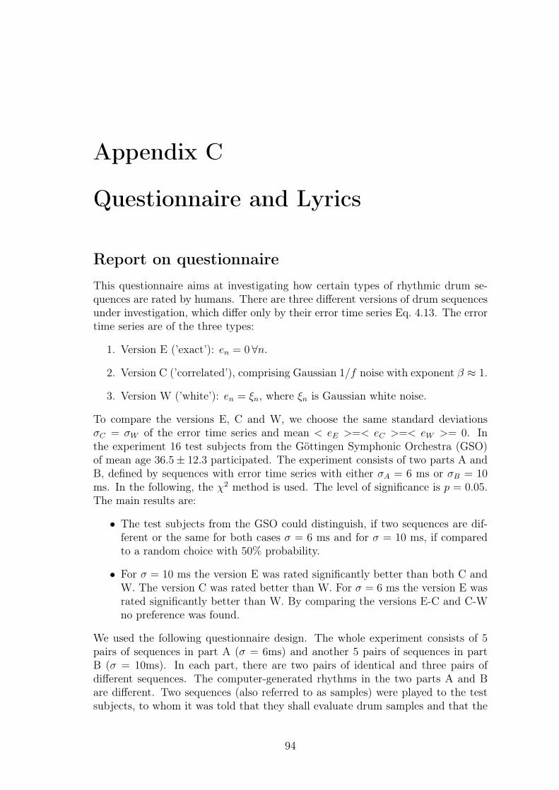
Concerning the project on music rhythms, first, I would like to thank Fabian Theis,Annette Witt and Jan Nagler for the fruitful collaboration and for stimulating dis-cussions. I wish to gratefully acknowledge the interdisciplinary collaboration withthe psychology department, in particular York Hagmayer, Anneke Fredebohm (whoinvestigated humanized music in her diploma thesis) and Christine Paulus. For thecreation of the humanized song, the wonderful team at Cubeaudio Recording Stu-dio deserves great thanks, also for providing audio data. Special thanks to Götzfor a highly creative collaboration – and for breakfast. I am also indebted to thepeople at Max-Planck-Innovation (in particular Bernd Ctortecka) and AlexanderBach for filing the patent and their enthusiasm and to the Göttingen SymphonicOrchestra (esp. Thomas Scholz).

I would like to thank everyone in the Geisel group for the great and lively atmo-sphere, from which I benefited a lot both scientifically and socially. Special thanksto Fabio and Jansky who have become friends. I would like to thank Marc Timmefor helpful discussions and his amity and my former and current office mates Anto-nio Méndez-Bermúdez, Raoul Martin Memmesheimer, Sven Jahnke and Rob Shawfor the friendly atmosphere and for their patience while I am writing up, and thetransport group – Oliver Bendix, Jakob Metzger and Kai Bröking for help and

useful discussions. For support concerning computer-related questions, I am in-debted to Denny Fliegner and Yorck-Fabian Beensen. I would like to thank KatjaFiedler and Lishma Anand as part of the midday “mtm” group and my gardenerbuddy with the “green thumb” Carsten Grabow. Thanks to Frank van Bussel forproofreading. I also want to thank the secretaries and the administrative staff. Iwish to acknowledge the head of the institutes management, Kerstin Mölter, forher support and enthusiasm. I wish to thank everyone who helped as a test person.

I would like to thank my friends for being who they are. I wish to thank my parentsand my brother for always being there for me. Finally, to Sabine, thank you foryour support, your smile and your patience.

To my parents

Contents

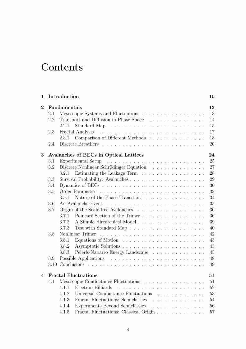
1 Introduction 10

2 Fundamentals 132.1 Mesoscopic Systems and Fluctuations . . . . . . . . . . . . . . . . . 132.2 Transport and Diffusion in Phase Space . . . . . . . . . . . . . . . 14

2.2.1 Standard Map . . . . . . . . . . . . . . . . . . . . . . . . . 152.3 Fractal Analysis . . . . . . . . . . . . . . . . . . . . . . . . . . . . 17

2.3.1 Comparison of Different Methods . . . . . . . . . . . . . . . 182.4 Discrete Breathers . . . . . . . . . . . . . . . . . . . . . . . . . . . 20

3 Avalanches of BECs in Optical Lattices 243.1 Experimental Setup . . . . . . . . . . . . . . . . . . . . . . . . . . 253.2 Discrete Nonlinear Schrödinger Equation . . . . . . . . . . . . . . 27

3.2.1 Estimating the Leakage Term . . . . . . . . . . . . . . . . . 283.3 Survival Probability: Avalanches . . . . . . . . . . . . . . . . . . . . 293.4 Dynamics of BECs . . . . . . . . . . . . . . . . . . . . . . . . . . . 303.5 Order Parameter . . . . . . . . . . . . . . . . . . . . . . . . . . . . 33

3.5.1 Nature of the Phase Transition . . . . . . . . . . . . . . . . 343.6 An Avalanche Event . . . . . . . . . . . . . . . . . . . . . . . . . . 353.7 Origin of the Scale-free Avalanches . . . . . . . . . . . . . . . . . . 36

3.7.1 Poincaré Section of the Trimer . . . . . . . . . . . . . . . . . 363.7.2 A Simple Hierarchical Model . . . . . . . . . . . . . . . . . . 393.7.3 Test with Standard Map . . . . . . . . . . . . . . . . . . . . 40

3.8 Nonlinear Trimer . . . . . . . . . . . . . . . . . . . . . . . . . . . . 423.8.1 Equations of Motion . . . . . . . . . . . . . . . . . . . . . . 433.8.2 Asymptotic Solutions . . . . . . . . . . . . . . . . . . . . . . 433.8.3 Peierls-Nabarro Energy Landscape . . . . . . . . . . . . . . 45

3.9 Possible Applications . . . . . . . . . . . . . . . . . . . . . . . . . 483.10 Conclusions . . . . . . . . . . . . . . . . . . . . . . . . . . . . . . . 49

4 Fractal Fluctuations 514.1 Mesoscopic Conductance Fluctuations . . . . . . . . . . . . . . . . 51

4.1.1 Electron Billiards . . . . . . . . . . . . . . . . . . . . . . . 524.1.2 Universal Conductance Fluctuations . . . . . . . . . . . . . 534.1.3 Fractal Fluctuations: Semiclassics . . . . . . . . . . . . . . 544.1.4 Experiments Beyond Semiclassics . . . . . . . . . . . . . . . 564.1.5 Fractal Fluctuations: Classical Origin . . . . . . . . . . . . . 57

8

4.1.5.1 Numerical Evidence . . . . . . . . . . . . . . . . . 574.1.5.2 Model: Open Standard Map . . . . . . . . . . . . . 584.1.5.3 Analytics: Fractal Dimension . . . . . . . . . . . . 604.1.5.4 Origin of the Power Law . . . . . . . . . . . . . . . 65

4.1.6 Conclusions . . . . . . . . . . . . . . . . . . . . . . . . . . . 654.2 Long-range Correlations in Music Rhythms . . . . . . . . . . . . . 67

4.2.1 Error Time Series . . . . . . . . . . . . . . . . . . . . . . . 684.2.2 Data Set & Analysis . . . . . . . . . . . . . . . . . . . . . . 704.2.3 Modeling Rhythmic Drumming . . . . . . . . . . . . . . . . 764.2.4 Humanizing Music Sequences . . . . . . . . . . . . . . . . . 78

4.2.4.1 Drum Rhythms . . . . . . . . . . . . . . . . . . . 794.2.4.2 Creating Humanized Music . . . . . . . . . . . . . 814.2.4.3 Perception of Humanized Music . . . . . . . . . . 824.2.4.4 Patent . . . . . . . . . . . . . . . . . . . . . . . . 83

4.2.5 Conclusions . . . . . . . . . . . . . . . . . . . . . . . . . . . 84

5 Conclusions and Outlook 86

Appendix 89

A Limiting Cases of the Participation Ratio 89

B Distribution of Islands (Mixed Phase Space) 91

C Questionnaire and Lyrics 94

D Audio Examples 97

Chapter 1

Introduction

The scientific and technological advances of the last decades have lead to the fab-rication of two different kinds of mesoscopic systems. On the one hand, in ascale-down approach, electrical and optical devices are shrunk to a degree whereintrinsic length scales of the material, such as the mean free path or the coherencelength, become comparable with the system size. Thus the actual shape of theconductor or the individual positions of impurities gain important roles and theencounter of classical nonlinear dynamics and interference effects lead to complexquantum dynamics. On the other hand in a scale-up approach microscopic unitsare assembled to form larger and more complex entities as in the growing field ofmolecular electronics, allowing to technologically use the phenomena of complexquantum dynamics.

A special type of this scaled up systems are Bose-Einstein condensates in opticaltraps and lattices, as they combine the acuteness of atomic systems with the flexi-bility and formability of solid state systems opening the new field of “atomtronics”.

All those mesoscopic systems have in common that either by their fabricationprocess or/and by their envisioned future function in some kind of circuitry, they arefundamentally coupled to the environment, so they have to be considered as opensystems. This led to a recent enhanced interest in the theory of open (quantum)systems and complex scattering.

Transport through these open systems is due to their mesoscopic nature proneto substantial fluctuations that can not be neglected or avoided and whose un-derstanding is thus a fundamental part of the theory of complex systems. In thiswork, we will encounter scale-free fluctuations in different kinds of complex non-linear systems.

In Chap. 3 we will see how nonlinear localization leads to scale-free fluctuationsin BECs in optical lattices in the framework of the discrete nonlinear Schrödingerequation (DNLS). We point out that although our focus is given to atomic BECs,our results are also relevant in a large variety of contexts (whenever the DNLS isadequate), most prominently in the light conduction in coupled nonlinear opticalwaveguides [1–5].

Experimentalists have achieved an extraordinary level of control over BECs inoptical traps in the past decade, which allows for the investigation of complex solidstate phenomena [6–13] and the emerging field of atomtronics promises a new gen-eration of nanoscale devices. It is therefore both of fundamental and technological

10

11

importance to understand the dynamics and transport properties of BECs in op-tical lattices. Here, we will show that if the optical lattice is opened at the ends,the statistics of the outgoing flux provides valuable and crucial information aboutthe internal dynamics of the system.

We will study the decay of an atomic BEC population N(τ) from the leakingboundaries of an optical lattice using a mean field description provided by theDNLS. The DNLS, which will be described in detail in Sec. 3.2, is a lattice equationthat contains a nonlinear term with prefactor Λ.

An exciting feature appearing in the framework of nonlinear lattices is theexistence of spatially localized, time-periodic and stable (or at least long-lived)excitations, termed discrete breathers (DBs), which emerge due to the nonlinearityand discreteness of the system. In the DNLS with boundary dissipation, we willsee that the internal systems dynamics evolves into generic initial conditions of DBstates for a nonlinearity larger than a threshold Λ > Λb, preventing the atoms fromreaching the leaking boundaries.

We show that collisions of other lattice excitations (e.g. “moving breathers”,see Sec. 2.4) with the outermost DBs result in bursts of the outflux of sizes δN ,i.e. steps in N(τ), which we call avalanches as for a whole range of Λ-values theyfollow a scale-free distribution, characterizing systems at a phase transition. Wewill see how the scale-free behavior reflects the complexity and the hierarchicalstructure of the underlying classical mixed phase space by reducing the system tofew degrees of freedom yielding the closed nonlinear trimer.

Furthermore, in this framework, we will investigate the collision process of astationary DB with a lattice excitation both analytically and numerically, whichis work that was started during a research visit at Boston University from May-September 2008.

While in Chap. 3 the transport properties of bosons in leaking optical latticesare described, in the first section of Chap. 4 we will consider fermions and discussthe electronic transport in open solid state mesoscopic systems. In these quantumsystems (such as quantum dots, nanowires etc.) fluctuations of the conductance,are a sensitive probe of electron dynamics and chaotic phenomena. A prominentfeature of electronic transport in mesoscopic systems is that the conductance as afunction of an external parameter, e.g. a gate voltage or a magnetic field, showsreproducible fluctuations caused by quantum interference [14–16].

A prediction from semiclassical theory that inspired a number of both theoreti-cal and experimental works in the fields of mesoscopic systems and quantum chaoswas that in chaotic systems with a mixed phase space these fluctuations wouldresult in fractal conductance curves [17, 18], i.e. when zooming into smaller andsmaller scales of changes of e.g. the magnetic field, the conductance curve remains“rough” in a self-affine way. Such fractal conductance fluctuations (FCF) have sincebeen confirmed in gold nanowires and in mesoscopic semiconductor quantum dotsin various experiments [19–23]. In addition, FCF have more recently been predictedto occur in strongly dynamically localized [24] and in diffusive systems [25].

We will explain, that the conductance of purely classical (i.e. incoherent) low-dimensional Hamiltonian systems very fundamentally exhibits fractal fluctuations,as long as transport is at least partially conducted by chaotic dynamics and that

12 CHAPTER 1. INTRODUCTION

the fractal dimension is governed by fundamental properties of chaotic dynamics.Thus mixed phase space systems and fully chaotic systems alike generally showfractal conductance fluctuations. This might explain the unexpected dependenceof the fractal dimension of the conductance curves on the (quantum) phase breakinglength observed in experiments on semiconductor quantum dots.

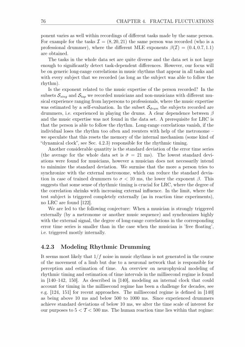
A completely different system where fractal fluctuations are found are musicrhythms played by humans (Sec. 4.2). While in the case of FCF, we are interestedin the structures on finer and finer scales, here the long-time correlations lead to thefractal nature of the fluctuations. Still, the idea of investigating human rhythmsemerged from studying FCF.

Music performed by humans will always exhibit a certain amount of fluctuationscompared with e.g. the steady beat of a metronome. It has been shown in the 1970sthat loudness and pitch fluctuations in music exhibit 1/fβ noise. Compositions inwhich the frequency and duration of each note were determined by 1/fβ noisesources sounded much more pleasing to listeners than those comprising white noisesources [26, 27].

We will show that the temporal fluctuations in simple as well as in more complexmusic rhythms are generic in the sense, that Gaussian 1/fβ noise is produced, nomatter if the rhythmic task is accomplished with hands, feet, a combination ofthese or the voice.

Moreover, we will be led to an application by asking the question: Does therhythmic structure of a piece of music sound better, when it is as exact as possibleor are long-range correlations more favorable? Professional contemporary audioediting software include a so called ’humanizing’ feature, which adds deviations ξn

to a given audio sequence, where ξn is white noise. Hence, there exists a desire tolet machine generated or modified music sound more natural. We created musicthat was humanized either with Gaussian 1/fβ noise or white noise. To furtherinvestigate the perception of natural deviations in human music rhythms withmore complex and realistic music pieces, an interdisciplinary diploma thesis inPsychology was initiated (Sec. 4.2.4.3).

The outline of the main part of the thesis is the following. In Chap. 2, somefundamental aspects of mesoscopic systems will be briefly reviewed. In Chap. 3,we will analyze Bose-Einstein condensates in leaking optical lattices described bythe DNLS yielding avalanches of ultracold atoms [28]. We will see that collisionsof DBs with other lattice excitations lead to the observed avalanches. The collisionprocess will be investigated analytically in the nonlinear trimer [29]. In the nextchapter, in Sec. 4.1, we consider fractal conductance fluctuations of classical originin mesoscopic systems [30]. Finally, in Sec. 4.2 we are dealing with generic long-range correlations in human rhythmic drumming [31, 32].

Chapter 2

Fundamentals

2.1 Mesoscopic Systems and FluctuationsIn this section we will introduce the notion of mesoscopic systems, see e.g. [33] for adetailed review. Much of solid state theory and statistical physics is concerned withthe properties of macroscopic systems. These are often considered while using thethermodynamic limit, i.e. the systems volume and particle number tend to infinitywhile their fraction remains constant. It is a convenient mathematical tool forobtaining bulk properties. Typically, the system approaches the macroscopic limitonce its size is much larger than relevant characteristic length scales, which are

• the coherence length, which is the distance a particle travels before its initialphase is destroyed,

• the de Broglie wavelength, which is related to the kinetic energy of the par-ticle,

• the mean free path, which is the distance that a particle travels before theinitial momentum is destroyed.

On the other hand, in the microscopic limit, we encounter systems such as singleatoms, where the laws of quantum mechanics govern the dynamics. Microscopicsystems are identical systems and the properties are exactly reproducible (e.g. thetransitions between energetic states in a hydrogen atom).

A mesoscopic system is a system in the intermediate size range between mi-croscopic and macroscopic. (mesos) from ancient Greek means "middle",the word mesoscopic was coined by Van Kampen in 1981. The size range of amesoscopic system depends on the relevant characteristic length scales (correlationlength, wavelength and mean free path), which vary widely from one material toanother and are also strongly affected by temperature, magnetic field etc. For thisreason, mesoscopic transport phenomena have been observed in conductors havinga wide range of dimensions from a few nanometers to hundreds of micrometers.

Statistical fluctuations of certain properties (e.g. the positions of impuritiesin semiconductor heterostructures) play an important role in mesoscopic systemsyielding to the notion that two mesoscopic samples are not identical though theymay belong to an ensemble which is describable in a statistical manner. The interest

13

14 CHAPTER 2. FUNDAMENTALS

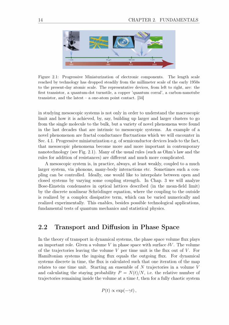
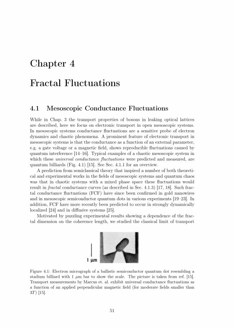
Figure 2.1: Progressive Miniaturization of electronic components. The length scalereached by technology has dropped steadily from the millimeter scale of the early 1950sto the present-day atomic scale. The representative devices, from left to right, are: thefirst transistor, a quantum-dot turnstile, a copper ’quantum corral’, a carbon-nanotubetransistor, and the latest – a one-atom point contact. [34]

in studying mesoscopic systems is not only in order to understand the macroscopiclimit and how it is achieved, by, say, building up larger and larger clusters to gofrom the single molecule to the bulk, but a variety of novel phenomena were foundin the last decades that are intrinsic to mesoscopic systems. An example of anovel phenomenon are fractal conductance fluctuations which we will encounter inSec. 4.1. Progressive miniaturization e.g. of semiconductor devices leads to the fact,that mesoscopic phenomena become more and more important in contemporarynanotechnology (see Fig. 2.1). Many of the usual rules (such as Ohm’s law and therules for addition of resistances) are different and much more complicated.

A mesoscopic system is, in practice, always, at least weakly, coupled to a muchlarger system, via phonons, many-body interactions etc. Sometimes such a cou-pling can be controlled. Ideally, one would like to interpolate between open andclosed systems by varying some coupling strength. In Chap. 3 we will analyzeBose-Einstein condensates in optical lattices described (in the mean-field limit)by the discrete nonlinear Schrödinger equation, where the coupling to the outsideis realized by a complex dissipative term, which can be varied numerically andrealized experimentally. This enables, besides possible technological applications,fundamental tests of quantum mechanics and statistical physics.

2.2 Transport and Diffusion in Phase Space

In the theory of transport in dynamical systems, the phase space volume flux playsan important role. Given a volume V in phase space with surface δV . The volumeof the trajectories leaving the volume V per time unit is the flux out of V . ForHamiltonian systems the ingoing flux equals the outgoing flux. For dynamicalsystems discrete in time, the flux is calculated such that one iteration of the maprelates to one time unit. Starting an ensemble of N trajectories in a volume V

and calculating the staying probability P = N(t)/N , i.e. the relative number oftrajectories remaining inside the volume at a time t, then for a fully chaotic system

P (t) ∝ exp(−γt) ,

2.2. TRANSPORT AND DIFFUSION IN PHASE SPACE 15

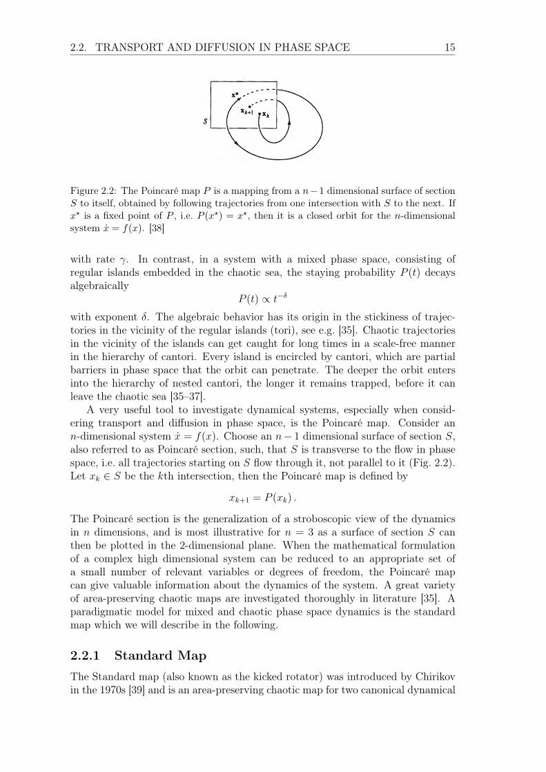
Figure 2.2: The Poincaré map P is a mapping from a n−1 dimensional surface of sectionS to itself, obtained by following trajectories from one intersection with S to the next. Ifx

� is a fixed point of P , i.e. P (x�) = x�, then it is a closed orbit for the n-dimensional

system x = f(x). [38]

with rate γ. In contrast, in a system with a mixed phase space, consisting ofregular islands embedded in the chaotic sea, the staying probability P (t) decaysalgebraically

P (t) ∝ t−δ

with exponent δ. The algebraic behavior has its origin in the stickiness of trajec-tories in the vicinity of the regular islands (tori), see e.g. [35]. Chaotic trajectoriesin the vicinity of the islands can get caught for long times in a scale-free mannerin the hierarchy of cantori. Every island is encircled by cantori, which are partialbarriers in phase space that the orbit can penetrate. The deeper the orbit entersinto the hierarchy of nested cantori, the longer it remains trapped, before it canleave the chaotic sea [35–37].

A very useful tool to investigate dynamical systems, especially when consid-ering transport and diffusion in phase space, is the Poincaré map. Consider ann-dimensional system x = f(x). Choose an n− 1 dimensional surface of section S,also referred to as Poincaré section, such, that S is transverse to the flow in phasespace, i.e. all trajectories starting on S flow through it, not parallel to it (Fig. 2.2).Let xk ∈ S be the kth intersection, then the Poincaré map is defined by

xk+1 = P (xk) .

The Poincaré section is the generalization of a stroboscopic view of the dynamicsin n dimensions, and is most illustrative for n = 3 as a surface of section S canthen be plotted in the 2-dimensional plane. When the mathematical formulationof a complex high dimensional system can be reduced to an appropriate set ofa small number of relevant variables or degrees of freedom, the Poincaré mapcan give valuable information about the dynamics of the system. A great varietyof area-preserving chaotic maps are investigated thoroughly in literature [35]. Aparadigmatic model for mixed and chaotic phase space dynamics is the standardmap which we will describe in the following.

2.2.1 Standard MapThe Standard map (also known as the kicked rotator) was introduced by Chirikovin the 1970s [39] and is an area-preserving chaotic map for two canonical dynamical


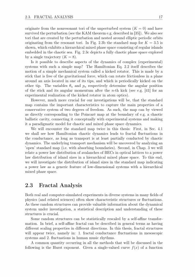
Figure 2.3: The KAM route to chaos generated with the standard map. (a) For relativelysmall nonlinearity (K = 0.55) many horizontally oriented KAM tori can be seen. (b)Mixed phase space (K = 3.5) with islands embedded in the chaotic sea. The enlargementsdemonstrate the hierarchical structure and immense complexity of a mixed phase space.(c) Fully chaotic phase space (K = 8). Shown is a single trajectory iterated for 50000time steps that explores the whole phase space area.

variables, e.g. momentum and angle (p,θ ). It is defined by the equations:

pn+1 = pn + K sin θn

θn+1 = θn + pn+1 (2.1)

Due to the periodicity of sin θ, the dynamics can be considered on a cylinder (bytaking θ mod 2π) or on a torus (by taking both θ, p mod 2π). The map is generatedby the time dependent Hamiltonian

H(p, θ, t) =p

2

2+ Kcosθ

∞�

n=0

δ(t− nT ) , (2.2)

where for simplicity we will set the period of the kicks T = 1. The dynamics is givenby a sequence of free propagations interleaved with periodic kicks. The standardmap goes through the whole KAM route to chaos in dependence of the nonlinearityparameter K [40]: From integrable (K = 0) via a mixed phase space to fully chaotic(K � 7). In Fig. 2.3 we are iterating a number of different initial conditions for along time. If the initial condition is on an invariant quasiperiodic torus, it tracesout the closed curve corresponding to the torus. If the initial condition yields achaotic orbit, then it will wander throughout an area densely filling that area. Wesee that for a relatively small perturbation K = 0.55, there are many KAM torirunning horizontally from θ = 0 to θ = 2π (Fig. 2.3a). These tori are those that

2.3. FRACTAL ANALYSIS 17

originate from the nonresonant tori of the unperturbed system (K = 0) and havesurvived the perturbation (see the KAM theorem e.g. described in [35]). We also seetori that are created by the perturbation and nested around elliptic periodic orbitsoriginating from the resonant tori. In Fig. 2.3b the standard map for K = 3.5 isshown, which exhibits a hierarchical mixed phase space consisting of regular islandsembedded in the chaotic sea. Fig. 2.3c depicts a fully chaotic phase space exploredby a single trajectory (K = 8).

Is it possible to describe aspects of the dynamics of complex (experimental)systems with such a simple map? The Hamiltonian Eq. 2.2 itself describes themotion of a simple mechanical system called a kicked rotator. This is made by astick that is free of the gravitational force, which can rotate frictionless in a planearound an axis located in one of its tips, and which is periodically kicked on theother tip. The variables θn and pn respectively determine the angular positionof the stick and its angular momentum after the n-th kick (see e.g. [41] for anexperimental realization of the kicked rotator in atom optics).

However, much more crucial for our investigations will be, that the standardmap contains the important characteristics to capture the main properties of aconservative system of two degrees of freedom. As such, the map can by viewedas directly corresponding to the Poincaré map at the boundary of e.g. a chaoticballistic cavity, connecting it conceptually with experimental systems and makingit a paradigmatic model for chaotic and mixed phase space dynamics.

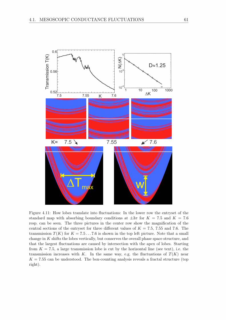
We will encounter the standard map twice in this thesis: First, in Sec. 4.1we shall see how Hamiltonian chaotic dynamics leads to fractal fluctuations inthe conductance, as long as transport is at least partially conducted by chaoticdynamics. The underlying transport mechanism will be uncovered by analyzing an’open’ standard map (i.e. with absorbing boundaries). Second, in Chap. 3 we willrelate a power law distribution of avalanches of BECs in optical lattices to a powerlaw distribution of island sizes in a hierarchical mixed phase space. To this end,we will investigate the distribution of island sizes in the standard map indicatinga power law as a generic feature of low-dimensional systems with a hierarchicalmixed phase space.

2.3 Fractal AnalysisBoth real and computer-simulated experiments in diverse systems in many fields ofphysics (and related sciences) often show characteristic structures or fluctuations.As these random structures can provide valuable information about the dynamicalsystem under investigation, a statistical description and understanding of thesestructures is crucial.

Some random structures can be statistically rescaled by a self-affine transfor-mation. In brief, a self-affine fractal can be described in general terms as havingdifferent scaling properties in different directions. In this thesis, fractal structureswill appear twice, namely in: 1. fractal conductance fluctuations in mesoscopicsystems and 2. fluctuations in human music rhythms.

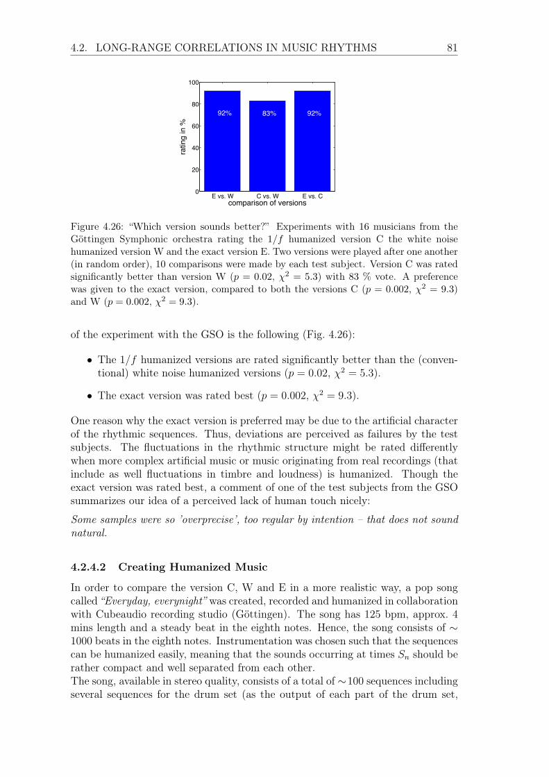
A common quantity occurring in all the methods that will be discussed in thefollowing is the Hurst exponent. Given a single-valued curve f(x) of a function


Figure 2.4: The construction of a simple, single-valued deterministic self-affine fractalcurve. (a) The generator consists of four line segments of equal length. (b-c) In thesecond and third stage, each of the four line segments has been replaced by a replica ofthe generator. The horizontal length is increased by a factor of 4 (i.e. sx = 4n), whilethe height is increased by a factor of 2 (i.e. sy = 2n). In the asymptotic limit, the fractalcurve f(x) can be scaled onto itself by sy = s

Hx with Hurst exponent H = 1/2. Figure

taken from [42].

f : R → R that is generated by a self-similar construction process, where n denotesthe generation index (see Fig. 2.4 for an illustrative example). A self-affine curvef(x) can be scaled onto itself by changing the horizontal length scale by a factor ofsx = a

n while the vertical length is rescaled by a factor of sy = bn, so that sy = s

H

x,

where H = logba is the Hurst exponent. The fractal dimension is related to theHurst exponent by

D = 2−H . (2.3)

In physics and related sciences, when fluctuations are found, typically the generatoror the construction process in not known. Hence, the self-similar properties of thethe fluctuations obtained are investigated in a statistical manner, for which a varietyof methods exists. In the following, we will overview several methods which areused to analyze fractal properties of fluctuations. For a detailed description seee.g. [42], a comparison of the methods is drawn in [43, 44].

2.3.1 Comparison of Different MethodsBox-Counting One of the most prominent approaches of fractal analysis is thebox-counting method. We will treat the 1 + 1-dimensional case, generalizationto higher dimensional manifolds is straightforward. Let N(s) be the number of

2.3. FRACTAL ANALYSIS 19

squares needed to cover the graph G ∈ R × R of a function f : R → R, where s

is the length of one side of a square. If N(s) behaves like a power law for smallenough s, the box-counting dimension Dbox is defined as

Dbox := lims→0

− ln N(s)

ln s. (2.4)

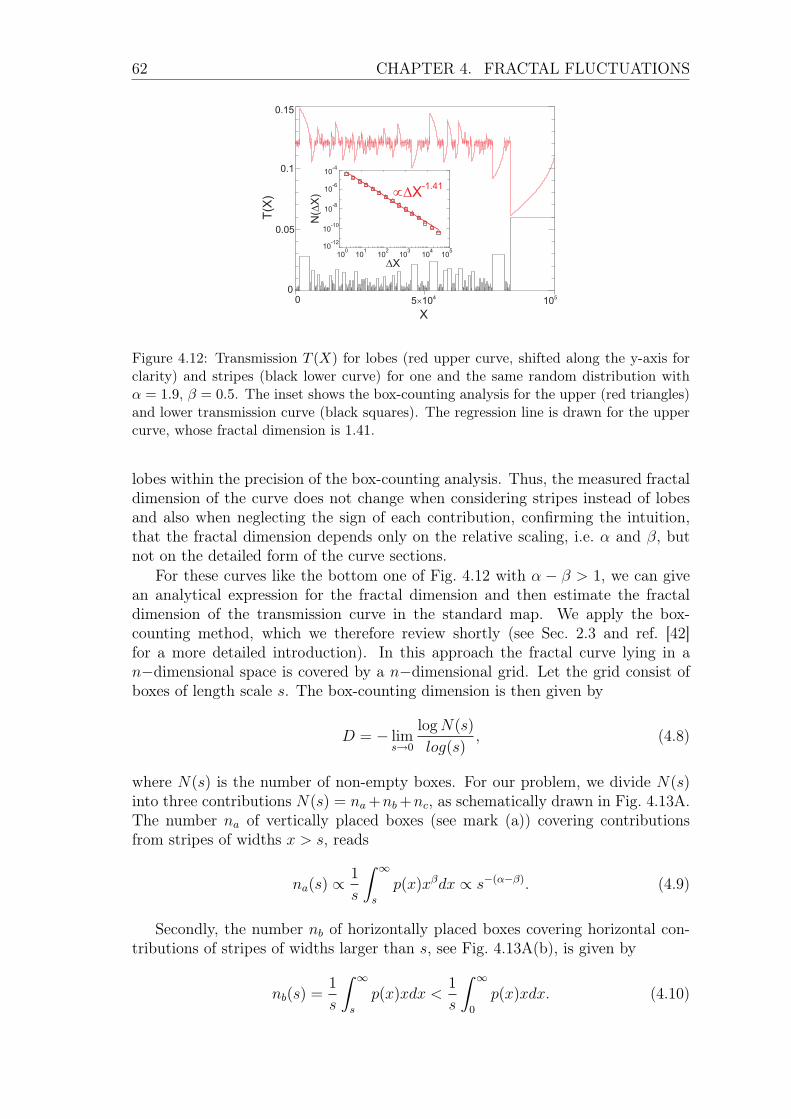
However, when applying the box-counting method numerically, caution has to betaken: Tests with fractal curves, where the Hurst exponent is known analytically(e.g. fractional Brownian motion or the Weierstrass-Mandelbrot series) show thatthe box-counting estimates are by far not the best and that other methods proveto be much more reliable [43]. In contrast, the box counting is very useful inthe analytical estimation of the fractal dimensionality of n-dimensional structures,notably when the generator or the underlying construction rule that leads to thestructure is known. We will apply the box counting method analytically to asequence of random transmission lobes in Sec. 4.1.5.3. For numerical estimates ofthe fractal dimension of conductance curves in Sec. 4.1, however, more suitable andreliable methods will be used as described in the following.

Variation Method and “Meakin Method” Given a mapping f : R → R. Thevariation method, described in [43], is based on the calculation of the maximumvariation v(x0, s) in a curve f(x) within a distance s of a point x0:

v(x0, s) = [sup f(x)− inf f(x)]|x0−x|<s . (2.5)

The “variation” V (s, f) of f(x) is defined as

V (s, f) =

�smax

0

v(x0, s)dx0 (2.6)

and the Hurst exponent is given by

H = lims→0

ln V (s)

ln(s). (2.7)

A similar method is proposed by Meakin [42] which consists simply of the heightdifference correlation function. A name was not found in literature, hence it willbe called the “Meakin method” in this thesis. The idea behind the method origi-nates in the observation, that in many important cases, a random self-affine frac-tal can be viewed of consisting of fluctuations about a straight reference line, inthis case given by the constant mean value. In this perspective, the Hurst expo-nent characterizes the relationship between the height differences of pairs of points(x1, f(x1), x2, f(x2)) of f(x) with respect to that reference line. For a self-affinecurve we find

< |f(x1)− f(x2)| >|x1−x2|=s ∼ sH

. (2.8)We tested both methods using the Weierstrass-Mandelbrot series and fractionalGaussian noise, where the Hurst exponent is known analytically. Both methodshave shown to be a much more reliable tool than e.g. the box-counting methodto numerically determine the fractal dimension of a graph G ∈ R× R and can beimplemented very efficiently. We will use these methods to estimate the fractaldimension of conductance curves (Sec. 4.1).


Detrended Fluctuation Analysis (DFA) The method of detrended fluctua-tion analysis, proposed in [45], has proven useful in revealing the extent of long-range correlations in time series. Similar to the Meakin method, fluctuations overa reference line are measured. However, in contrast to the Meakin method, thereference line is given by the local trend, i.e. the data is divided into boxes anddetrended locally. More specifically, DFA involves a detrending of the data in theboxes using a polynomial of degree m, e.g. for linear and quadratic detrending themethod is referred to as DFA1 and DFA2 respectively. We will describe DFA1,extension to DFA2, DFA3 etc. is straightforward.

Given a time series f(t) of total length N to be analyzed. First, the time seriesis integrated yielding

y(k) =k�

t=1

f(t) .

The integrated time series is divided into boxes of equal length, s. In each box,a least squares line ys(k) is fitted to the data (representing the linear trend inthat box), see Fig. 4.20. Next, we detrend the integrated time series, y(k), bysubtracting the local trend, ys(k), in each box. The root-mean-square fluctuationof this detrended time series is calculated by

F (s) =< y(k)− ys(k) >=

�� 1

N

N�

k=1

y(k)− ys(k) (2.9)

This computation is repeated over the time scales (box sizes) of interest to char-acterize the relationship between the average fluctuation F (s), and the box size s.A linear relationship on a log-log plot indicates the presence of power law (frac-tal) scaling F (s) ∼ s

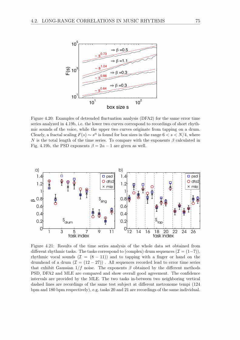
α with scaling exponent α. For fractional Gaussian noise theexponent α is equal to the Hurst exponent α = H, while for fractional Brownianmotion α = H−1. We will use DFA to analyze error time series of rhythmic musicsequences played by humans in Sec. 4.2.

2.4 Discrete BreathersAn important and exciting feature appearing in the frame of nonlinear latticesare discrete breathers (DBs), which we will encounter in Chap. 3. The followingworking definition is taken from [46] (see as well [47, 48] for an overview):

”Discrete breathers (DB) or intrinsic localized modes are spatially localized,time-periodic, stable (or at least long-lived) excitations in spatially extended per-fectly periodic discrete systems.”

The phenomenon of localization of, e.g. energy or particles is well known in solidstate physics. Typical examples are the localized vibrational phonon modes aroundimpurities or defects in crystals and Anderson localization of electrons in disorderedmedia. Localization is usually perceived as arising from external disorder, e.g. inthe case of Anderson localization, that breaks the discrete translational invarianceof a perfect crystal lattice. In contrast, in the late 1980s it was found that intrinsic

2.4. DISCRETE BREATHERS 21

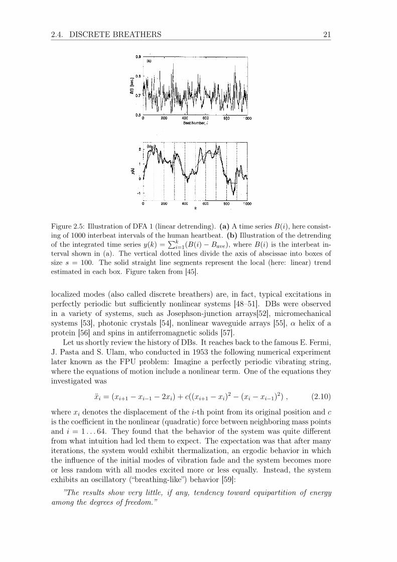
Figure 2.5: Illustration of DFA 1 (linear detrending). (a) A time series B(i), here consist-ing of 1000 interbeat intervals of the human heartbeat. (b) Illustration of the detrendingof the integrated time series y(k) =

�k

i=1(B(i) − Bave), where B(i) is the interbeat in-terval shown in (a). The vertical dotted lines divide the axis of abscissae into boxes ofsize s = 100. The solid straight line segments represent the local (here: linear) trendestimated in each box. Figure taken from [45].

localized modes (also called discrete breathers) are, in fact, typical excitations inperfectly periodic but sufficiently nonlinear systems [48–51]. DBs were observedin a variety of systems, such as Josephson-junction arrays[52], micromechanicalsystems [53], photonic crystals [54], nonlinear waveguide arrays [55], α helix of aprotein [56] and spins in antiferromagnetic solids [57].

Let us shortly review the history of DBs. It reaches back to the famous E. Fermi,J. Pasta and S. Ulam, who conducted in 1953 the following numerical experimentlater known as the FPU problem: Imagine a perfectly periodic vibrating string,where the equations of motion include a nonlinear term. One of the equations theyinvestigated was

xi = (xi+1 − xi−1 − 2xi) + c((xi+1 − xi)2 − (xi − xi−1)

2) , (2.10)

where xi denotes the displacement of the i-th point from its original position and c

is the coefficient in the nonlinear (quadratic) force between neighboring mass pointsand i = 1 . . . 64. They found that the behavior of the system was quite differentfrom what intuition had led them to expect. The expectation was that after manyiterations, the system would exhibit thermalization, an ergodic behavior in whichthe influence of the initial modes of vibration fade and the system becomes moreor less random with all modes excited more or less equally. Instead, the systemexhibits an oscillatory (“breathing-like”) behavior [59]:

”The results show very little, if any, tendency toward equipartition of energyamong the degrees of freedom.”


Figure 2.6: (left) Frequency versus wavenumber plane shows the spectrum of linear os-cillations and two isolated frequencies ωb outside the linear spectrum corresponding todiscrete breathers [46]. The red circles indicate the amplitudes (e.g. particle displace-ments) for the DB solution. (right) The discrete nonlinear Schrödinger equation (seeSec. 3.2) rigorously exhibits discrete breathers [58].

This (at first sight) puzzling computer experiment leads to the question: How canlocalization arise in a perfectly periodic lattice and what makes a DB stable? Linearexcitations – be they electrons or phonons – moving through a solid will experiencea periodic energy potential, which implies by the Bloch theorem the existence of’forbidden’ and ’allowed’ bands of frequency and velocity for their motion. Linearexcitations can propagate through the solid only in the allowed bands which havea highest and a lowest frequency. The situation is different for nonlinear excita-tions. As can be seen from the simple one dimensional pendulum, the frequency isindependent of the amplitude when linearizing the equations of motion, but doesdepend on the amplitude in the nonlinear (high amplitude) regime. If a large am-plitude (and hence nonlinear) excitation is created – a possible candidate for adiscrete breather – it’s frequency can lie outside the allowed band of linear excita-tions (see Fig. 2.6). The highest frequency of the allowed band is determined bythe degree of discreteness of the lattice: The larger the lattice constant, the smallerthe highest frequency of the linear band. If all harmonics of the DB frequency lieoutside (above) the allowed band, then the DB cannot couple to linear excitationsand is therefore stable against decaying into them. To summarize, a DB is a local-ized oscillatory excitation that is stabilized against decay by the discreteness of anonlinear periodic lattice. The stability of DBs in BECs will play a crucial role inChap. 3.

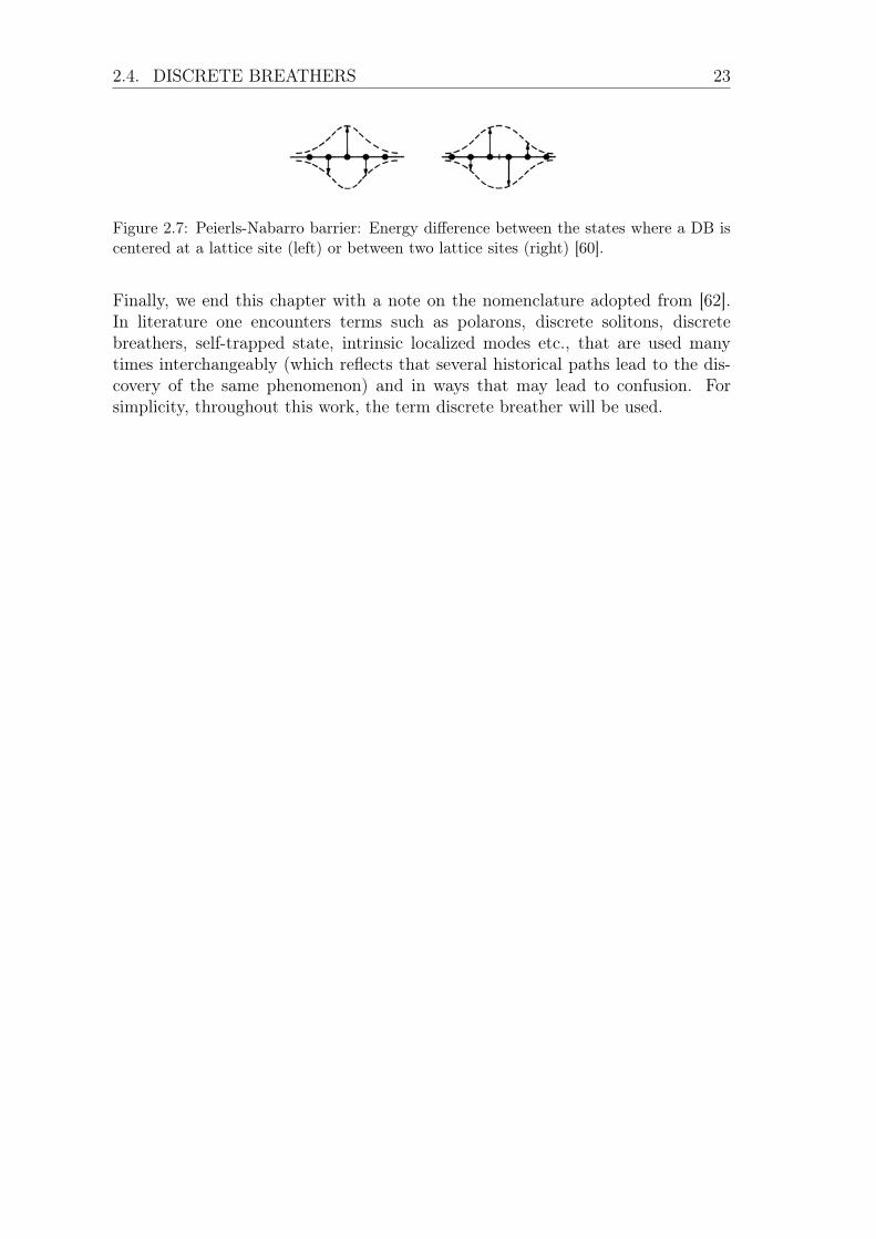
A quantity related to DBs is the Peierls-Nabarro barrier, which is given by theenergy difference |Ec−Eb|, where Ec and Eb are the energies for a DB centered ata lattice site or between two lattice sites [60, 61], see Fig. 2.7.

2.4. DISCRETE BREATHERS 23

Figure 2.7: Peierls-Nabarro barrier: Energy difference between the states where a DB iscentered at a lattice site (left) or between two lattice sites (right) [60].

Finally, we end this chapter with a note on the nomenclature adopted from [62].In literature one encounters terms such as polarons, discrete solitons, discretebreathers, self-trapped state, intrinsic localized modes etc., that are used manytimes interchangeably (which reflects that several historical paths lead to the dis-covery of the same phenomenon) and in ways that may lead to confusion. Forsimplicity, throughout this work, the term discrete breather will be used.

Chapter 3

Avalanches of BECs in Optical

Lattices

One of the most fascinating experimental achievements of the last decade was un-ambiguously the realization of Bose-Einstein Condensation (BEC) of ultra-coldatoms in optical lattices (OLs) [6, 63–66]. Experimentalists have achieved an ex-traordinary level of control over BECs in optical traps in the past decade, whichallows for the investigation of complex solid state phenomena [6–13] and the emerg-ing field of “atomtronics” promises a new generation of nanoscale devices such asan atom laser. The atom laser, a bright, coherent matter wave derived from aBose-Einstein condensate holds great promise for precision measurement and forfundamental tests of quantum mechanics. It is therefore both of fundamental andtechnological importance to understand the dynamics and transport properties ofBECs in OLs. We ask the following question: What are the transport propertiesof BECs in leaking optical lattices and can we understand the statistics of theoutgoing flux of ultracold bosons?

We study the decay of an atomic BEC population N(τ) from the leaking bound-aries of an optical lattice using a mean field description provided by the discretenonlinear Schrödinger equation (DNLS). The DNLS, described in detail in Sec. 3.2,is a lattice equation that contains a nonlinearity Λ. An exciting feature appearingin nonlinear lattices is the existence of discrete breathers (DBs), which are spa-tially localized, time-periodic and stable (or at least long-lived) excitations. DBsemerge due to the nonlinearity and discreteness of the system (Historically, theFermi-Pasta-Ulam problem lead to the discovery of discrete breathers in the 1950s,see Sec. 2.4 for an introduction). DBs were observed in various experimental se-tups [3, 52, 55, 67–74] while their existence and stability were studied thoroughlyduring the last decade [46, 48, 49, 51, 75–79]. It was shown that they act as virtualbottlenecks which slow down the relaxation processes in generic nonlinear lattices[51, 78–81]. Further works [82–86] established the fact that absorbing boundariescan take generic initial conditions towards DBs.

In the DNLS with dissipation at the ends of the lattice, we find that the dynam-ics evolves into the population of discrete breathers for a nonlinearity larger thana threshold Λ > Λb preventing the atoms from reaching the leaking boundaries.We show that collisions of other lattice excitations (e.g. a moving breather, seeSec. 2.4) with the outermost DBs result in avalanches, i.e. steps in N(τ), which for

24

3.1. EXPERIMENTAL SETUP 25

a whole range of Λ−values follow a scale-free distribution [28]

P(J = δN) ∼ 1/Jα

characterizing systems at a phase transition. We will see that the scale-free behaviorof P(J) reflects the complexity and the hierarchical structure of the underlyingclassical mixed phase space of the trimer. A theoretical analysis of the mixedphase space of the system indicates that 1 < α < 3 in agreement with our numericalfindings.

We propose an order parameter to describe the observed phase transition.Though we do have clear numerical evidence concerning the phase transition, anunderstanding of the phase transition together with an analytical expression for Λb

is still an open and fascinating question and work in progress [87]. The collisionprocess of a stationary breather with a moving breather is analyzed analyticallyand numerically in a reduced system consisting of 3 lattice sites, called the non-linear trimer [29] (by means of the local ansatz [49] described in Sec. 3.6). Wepoint out that although our focus is given to atomic BECs, our results are alsorelevant in a large variety of contexts (whenever the DNLS is adequate), mostprominently being the light emittance from coupled nonlinear optical waveguides[1–5, 54, 55, 74, 88–92], see Sec. 3.9 for more details on discrete breathers in opticalwaveguide arrays.

3.1 Experimental SetupWe consider the statistics of emitted ultracold atoms from an OL with leakage atthe edges. Typically, ultracold atoms are stored in magnetic dipole traps, thatmake use of the interaction between an induced dipole moment in an atom andan external electric field provided by a laser. A periodic potential can then beformed by overlapping two counter-propagating laser beams as shown in Fig. 3.1.The magnetic field gives rise to a harmonic trapping potential which confines thecondensate in an array of tightly confining 1D potential tubes, for our purposeswith its long axis oriented perpendicular to the gravitational force. Along the 1Dtubes, a periodic potential can be created (again with two counter-propagatinglaser beams) leading to a 1D optical lattice (Fig. 3.2a). The depths of the opticalpotential, i.e. the tunneling amplitude between the lattice sites, can be varied bychanging the intensity of the laser light.

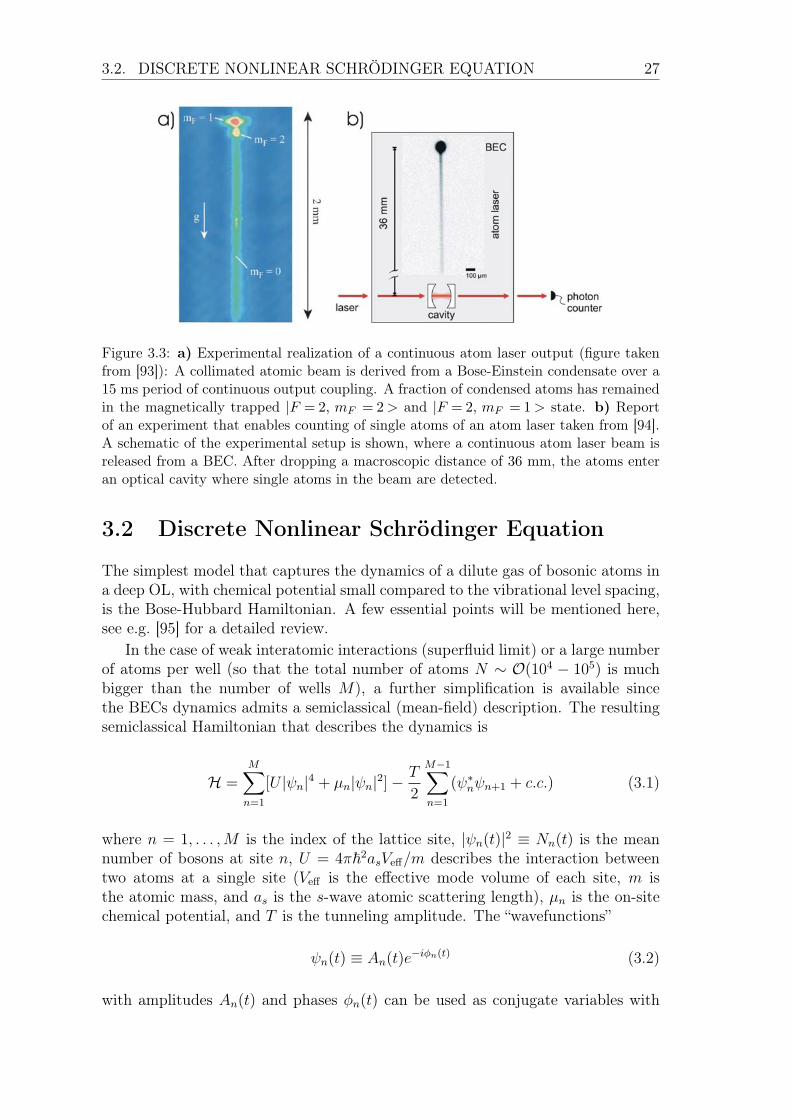
The leakage can be realized experimentally by applying two separate continuousmicrowave fields or Raman lasers at the edges of the sample to locally spin-flipthe atoms inside the BEC to an untrapped state [58, 86, 93, 94]1. The spin-flipped atoms do not experience the magnetic trapping potential, and hence theyare released through gravity at the ends of the OL ( Fig. 3.2b). An experimentalrealization of a continuous output of atoms is shown in Fig. 3.3a, where a field withfrequency ν induces transitions from the magnetically trapped |F = 2, mF = 2 >

state to the untrapped |F =2, mF =0> state via the |F =2, mF =1> state. Here,

1Spatially localized microwave fields focused below the wavelength can be obtained at the tip

of tapered waveguides.

26 CHAPTER 3. AVALANCHES OF BECS IN OPTICAL LATTICES

F denotes the total angular momentum and mF is the magnetic quantum number.The resonance condition reads 1

2µB|B(r)| = hν, where µB is the Bohr magneton.An experimental realization of the time-resolved counting of the released atomsis shown in Fig. 3.3b [94]. Thus, an accurate monitoring of the decay process ofthe atomic population can be utilized to probe the dynamical properties of BECsinside an optical lattice.

Figure 3.1: a) Optical lattice potentials formed by superimposing two orthogonal standingwaves [66]. b) For a 2D optical lattice, the atoms are confined to an array of tightlyconfining 1D potential tubes (in this picture of 15 µm length and 60 nm width). Thepicture is taken from www.quantumoptics.ethz.ch.

Figure 3.2: a) Illustration (taken from [66]) of BECs loaded in an optical lattice. Thestanding-wave interference pattern creates a periodic potential in which the atoms moveby tunnel coupling between the individual wells. b) Schematic realization of leakage atthe two edges of the lattice using continuous microwave or Raman lasers to spin-flip atomsthat reach the edges to a untrapped state (Figure taken from [86]). Thus, the atoms atthe edges do not experience the magnetic trapping and hence are released through gravity.The released atoms are then measured at the detectors.

3.2. DISCRETE NONLINEAR SCHRÖDINGER EQUATION 27

Figure 3.3: a) Experimental realization of a continuous atom laser output (figure takenfrom [93]): A collimated atomic beam is derived from a Bose-Einstein condensate over a15 ms period of continuous output coupling. A fraction of condensed atoms has remainedin the magnetically trapped |F = 2, mF = 2 > and |F = 2, mF = 1 > state. b) Reportof an experiment that enables counting of single atoms of an atom laser taken from [94].A schematic of the experimental setup is shown, where a continuous atom laser beam isreleased from a BEC. After dropping a macroscopic distance of 36 mm, the atoms enteran optical cavity where single atoms in the beam are detected.

3.2 Discrete Nonlinear Schrödinger Equation

The simplest model that captures the dynamics of a dilute gas of bosonic atoms ina deep OL, with chemical potential small compared to the vibrational level spacing,is the Bose-Hubbard Hamiltonian. A few essential points will be mentioned here,see e.g. [95] for a detailed review.

In the case of weak interatomic interactions (superfluid limit) or a large numberof atoms per well (so that the total number of atoms N ∼ O(104 − 105) is muchbigger than the number of wells M), a further simplification is available sincethe BECs dynamics admits a semiclassical (mean-field) description. The resultingsemiclassical Hamiltonian that describes the dynamics is

H =M�

n=1

[U |ψn|4 + µn|ψn|2]−T

2

M−1�

n=1

(ψ∗nψn+1 + c.c.) (3.1)

where n = 1, . . . ,M is the index of the lattice site, |ψn(t)|2 ≡ Nn(t) is the meannumber of bosons at site n, U = 4π�2

asVeff/m describes the interaction betweentwo atoms at a single site (Veff is the effective mode volume of each site, m isthe atomic mass, and as is the s-wave atomic scattering length), µn is the on-sitechemical potential, and T is the tunneling amplitude. The “wavefunctions”

ψn(t) ≡ An(t)e−iφn(t) (3.2)

with amplitudes An(t) and phases φn(t) can be used as conjugate variables with


respect to the Hamiltonian iH leading to a set of canonical equations

i∂ψn

∂t=

∂H∂ψ∗

n

i∂ψ

∗n

∂t= − ∂H

∂ψn

(3.3)

which upon evaluation yields the Discrete Nonlinear Schrödinger Equation (DNLS)

i∂ψn

∂τ= λ(|ψn|2 + µn)ψn −

1

2[ψn−1 + ψn+1]; n = 1, . . . ,M . (3.4)

Here, λ = 2U/T is the nonlinearity and τ = Tt is the normalized time.The DNLS can be applied to a remarkably large variety of systems, examples

include Davydov’s model for energy transport in biomolecules, or the theory oflocal modes of small molecules [96] and within nonlinear optics it is a model ofcoupled nonlinear waveguides [1]. In particular this mathematical model describes(in the mean-field limit) the dynamics of a BEC in a leaking OL of size M [97].We will treat the repulsive case explicitly (λ > 0), however, the attractive case canbe obtained via the staggering transformation ψn → (−1n)ψn [48]. To simulate theoutput coupling of atoms at the boundaries of our 1D lattice, we supplement thestandard DNLS with local dissipation terms at the two edges of the lattice [58, 86].The resulting equation reads:

i∂ψn

∂τ= Λ|ψn|2ψn −

1

2[ψn−1 + ψn+1]− iγψn[δn,1 + δn,M ]; n = 1, . . . ,M , (3.5)

where γ is the dissipation rate and we defined an initial effective (rescaled) inter-atomic interaction per site

Λ = λρ, (3.6)with ρ = N(t = 0)/M being the initial average density of atoms in the OL, so thatfor different lattice sizes M , we maintain the same local dynamics by keeping Λconstant. In Eq. 3.5 we have set µn = 0∀n, i.e. static disorder will not be treatedin the following. The time t, the interatomic interaction λ, and the atom emissionprobability γ describing atomic losses from the boundary of the OL are measuredin units of the tunneling rate T . In an experimental setup, T can be adjusted bythe intensity of the standing laser wave field and the on-site interaction U dependson the confining potential perpendicular to the tube in which the atoms move.Thus, the nonlinearity λ can be varied experimentally.

3.2.1 Estimating the Leakage TermIn order to be able to compare with experiments, especially with BECs in leakingOLs, the dissipation rate γ will be estimated within a mean-field approximation[86]. Here, we consider the case of two output-coupler fields interacting with theatoms at the first and last lattice wells only. We can describe the output couplingthrough an external reservoir formed by an infinite number of states [86]. Foroptical input-output theory and in proposed atom laser theories that result in Born-Markov master equations, typically κ(k) = const. is chosen (broadband coupling)

3.3. SURVIVAL PROBABILITY: AVALANCHES 29

[98], where the function κ(k) describes the shape of the (output) coupling in k space.For a broadband output coupling κ the Born-Markov approximation leading to anexponentially decaying atomic density inside the BEC should satisfy [98]

ω3/2

πκ2

��

2m� 1 (3.7)

where ω is the 1D trapping frequency and m is the atomic mass. And on the otherhand, the characteristic decay time is given by

tD =1

πκ2

�2ω�m

=�/T

γ, (3.8)

leading to

γ =πκ

2√

�m

T√

2ω. (3.9)

Eq. 3.9 shows the proportionality between the dissipation rate γ and the squareof the coupling strength κ and gives (together with Eq. 3.7) a condition on themagnitude of the dissipation rate γ in order for the Born-Markov approximationto be valid:

�ω

2γT� 1 . (3.10)

Using typical parameter values of experiments of BECs in optical lattices, whichare �/T ≈ 6 × 10−4 and ω ≈ 80 kHz [7], the above condition is fulfilled up toγ ≈ 0.5. The results for the leaking system reported below are for a dissipationrate of γ = 0.2. Nevertheless, we have checked that the qualitative behavior is thesame for other values of γ < 0.5. For larger values of γ, non-Markovian terms haveto be included in the description [99].

3.3 Survival Probability: AvalanchesLet us now study the decay and the statistical properties of the total atomic pop-ulation inside the OL (also referred to as survival probability or total norm)

N (τ) =N(τ)

N(0)=

M�

n=1

|ψn(τ)|2, (3.11)

where we normalized the wave functions such that

N(t=0)=1 . (3.12)

Its time derivative −dN(τ)dτ

is equal to the outgoing atomic flux. In our numericalexperiments we have used initial conditions with randomly distributed phases forthe wavefunctions ψn = An exp(−iφn), while Nn(τ = 0) was taken to be almostconstant with only small random fluctuations across the OL. The initial stateswere first “thermalized” during a conservative (i.e. γ =0) transient period of, typi-cally, τ =500. Only after this transient is completed, the dissipation at the lattice


boundaries is switched on, leading to a progressive loss of atoms. The dynami-cal evolution is done through numerical integration by the Runge-Kutta-Fehlbergmethod with an accuracy such that for the largest system studied (M = 4096)deviations of N (τ) from unity in a closed system (γ = 0) were less than 10−4 forthe total time range studied (t ≤ 30000).

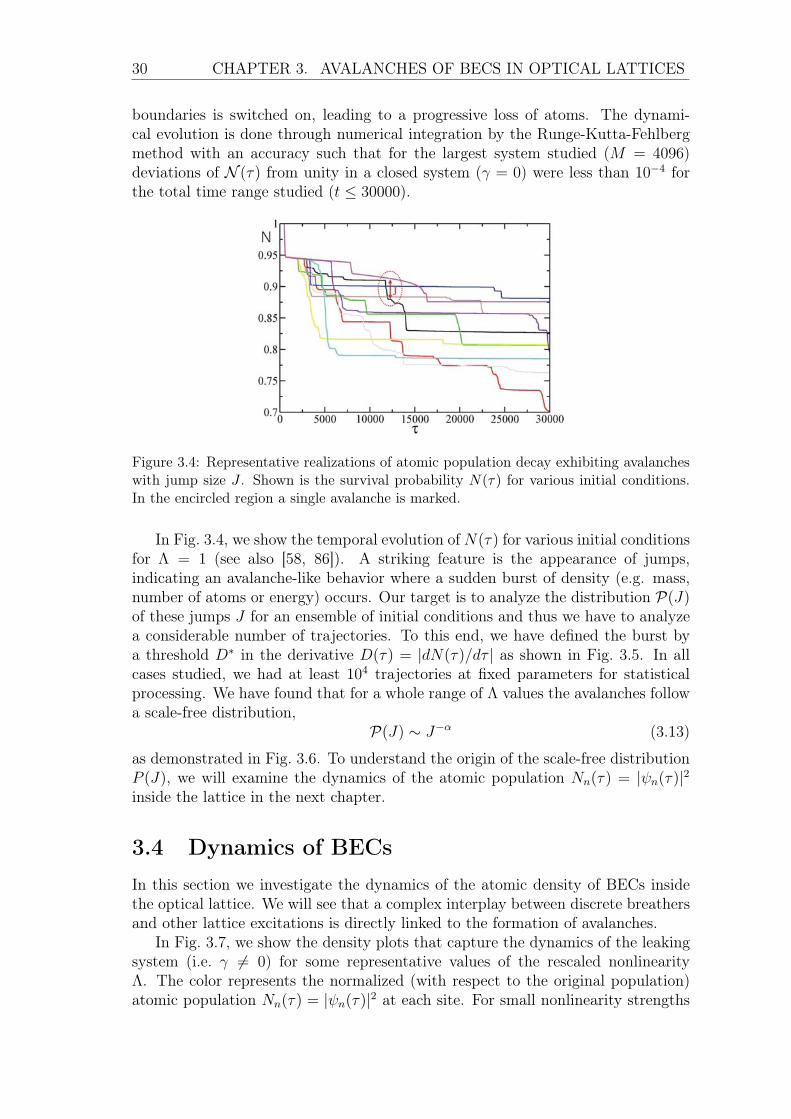
Figure 3.4: Representative realizations of atomic population decay exhibiting avalancheswith jump size J . Shown is the survival probability N(τ) for various initial conditions.In the encircled region a single avalanche is marked.

In Fig. 3.4, we show the temporal evolution of N(τ) for various initial conditionsfor Λ = 1 (see also [58, 86]). A striking feature is the appearance of jumps,indicating an avalanche-like behavior where a sudden burst of density (e.g. mass,number of atoms or energy) occurs. Our target is to analyze the distribution P(J)of these jumps J for an ensemble of initial conditions and thus we have to analyzea considerable number of trajectories. To this end, we have defined the burst bya threshold D

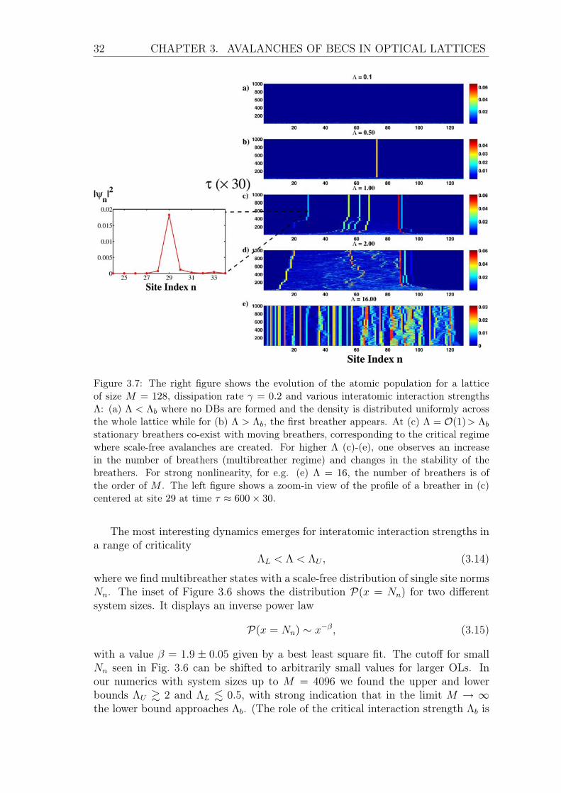
∗ in the derivative D(τ) = |dN(τ)/dτ | as shown in Fig. 3.5. In allcases studied, we had at least 104 trajectories at fixed parameters for statisticalprocessing. We have found that for a whole range of Λ values the avalanches followa scale-free distribution,

P(J) ∼ J−α (3.13)

as demonstrated in Fig. 3.6. To understand the origin of the scale-free distributionP (J), we will examine the dynamics of the atomic population Nn(τ) = |ψn(τ)|2inside the lattice in the next chapter.

3.4 Dynamics of BECsIn this section we investigate the dynamics of the atomic density of BECs insidethe optical lattice. We will see that a complex interplay between discrete breathersand other lattice excitations is directly linked to the formation of avalanches.

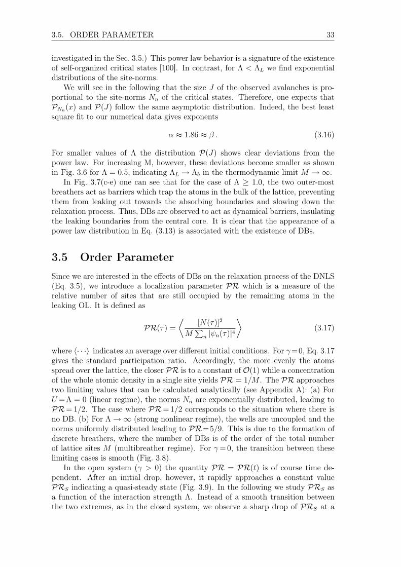
In Fig. 3.7, we show the density plots that capture the dynamics of the leakingsystem (i.e. γ �= 0) for some representative values of the rescaled nonlinearityΛ. The color represents the normalized (with respect to the original population)atomic population Nn(τ) = |ψn(τ)|2 at each site. For small nonlinearity strengths

3.4. DYNAMICS OF BECS 31

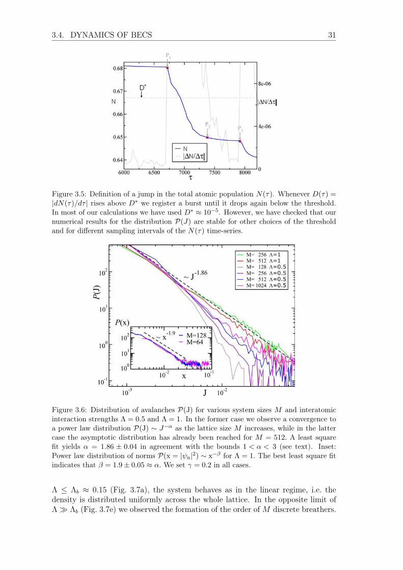
Figure 3.5: Definition of a jump in the total atomic population N(τ). Whenever D(τ) =|dN(τ)/dτ | rises above D

∗ we register a burst until it drops again below the threshold.In most of our calculations we have used D

∗ ≈ 10−5. However, we have checked that ournumerical results for the distribution P(J) are stable for other choices of the thresholdand for different sampling intervals of the N(τ) time-series.

Figure 3.6: Distribution of avalanches P(J) for various system sizes M and interatomicinteraction strengths Λ = 0.5 and Λ = 1. In the former case we observe a convergence toa power law distribution P(J) ∼ J

−α as the lattice size M increases, while in the lattercase the asymptotic distribution has already been reached for M = 512. A least squarefit yields α = 1.86 ± 0.04 in agreement with the bounds 1 < α < 3 (see text). Inset:Power law distribution of norms P(x = |ψn|2) ∼ x−β for Λ = 1. The best least square fitindicates that β = 1.9± 0.05 ≈ α. We set γ = 0.2 in all cases.

Λ ≤ Λb ≈ 0.15 (Fig. 3.7a), the system behaves as in the linear regime, i.e. thedensity is distributed uniformly across the whole lattice. In the opposite limit ofΛ � Λb (Fig. 3.7e) we observed the formation of the order of M discrete breathers.


Figure 3.7: The right figure shows the evolution of the atomic population for a latticeof size M = 128, dissipation rate γ = 0.2 and various interatomic interaction strengthsΛ: (a) Λ < Λb where no DBs are formed and the density is distributed uniformly acrossthe whole lattice while for (b) Λ > Λb, the first breather appears. At (c) Λ = O(1)> Λb

stationary breathers co-exist with moving breathers, corresponding to the critical regimewhere scale-free avalanches are created. For higher Λ (c)-(e), one observes an increasein the number of breathers (multibreather regime) and changes in the stability of thebreathers. For strong nonlinearity, for e.g. (e) Λ = 16, the number of breathers is ofthe order of M . The left figure shows a zoom-in view of the profile of a breather in (c)centered at site 29 at time τ ≈ 600× 30.

The most interesting dynamics emerges for interatomic interaction strengths ina range of criticality

ΛL < Λ < ΛU , (3.14)

where we find multibreather states with a scale-free distribution of single site normsNn. The inset of Figure 3.6 shows the distribution P(x = Nn) for two differentsystem sizes. It displays an inverse power law

P(x = Nn) ∼ x−β

, (3.15)

with a value β = 1.9 ± 0.05 given by a best least square fit. The cutoff for smallNn seen in Fig. 3.6 can be shifted to arbitrarily small values for larger OLs. Inour numerics with system sizes up to M = 4096 we found the upper and lowerbounds ΛU � 2 and ΛL � 0.5, with strong indication that in the limit M → ∞the lower bound approaches Λb. (The role of the critical interaction strength Λb is

3.5. ORDER PARAMETER 33

investigated in the Sec. 3.5.) This power law behavior is a signature of the existenceof self-organized critical states [100]. In contrast, for Λ < ΛL we find exponentialdistributions of the site-norms.

We will see in the following that the size J of the observed avalanches is pro-portional to the site-norms Nn of the critical states. Therefore, one expects thatPNn(x) and P(J) follow the same asymptotic distribution. Indeed, the best leastsquare fit to our numerical data gives exponents

α ≈ 1.86 ≈ β . (3.16)

For smaller values of Λ the distribution P(J) shows clear deviations from thepower law. For increasing M, however, these deviations become smaller as shownin Fig. 3.6 for Λ = 0.5, indicating ΛL → Λb in the thermodynamic limit M →∞.

In Fig. 3.7(c-e) one can see that for the case of Λ ≥ 1.0, the two outer-mostbreathers act as barriers which trap the atoms in the bulk of the lattice, preventingthem from leaking out towards the absorbing boundaries and slowing down therelaxation process. Thus, DBs are observed to act as dynamical barriers, insulatingthe leaking boundaries from the central core. It is clear that the appearance of apower law distribution in Eq. (3.13) is associated with the existence of DBs.

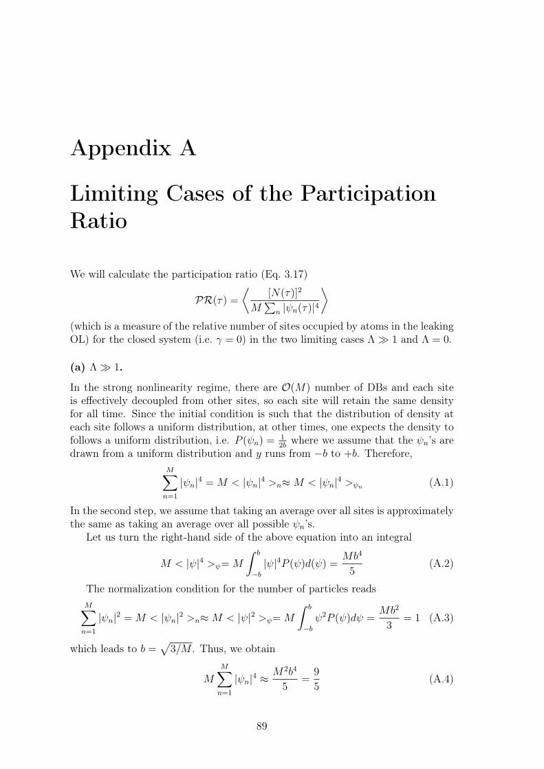
3.5 Order ParameterSince we are interested in the effects of DBs on the relaxation process of the DNLS(Eq. 3.5), we introduce a localization parameter PR which is a measure of therelative number of sites that are still occupied by the remaining atoms in theleaking OL. It is defined as

PR(τ) =

�[N(τ)]2

M�

n|ψn(τ)|4

�(3.17)

where �· · ·� indicates an average over different initial conditions. For γ =0, Eq. 3.17gives the standard participation ratio. Accordingly, the more evenly the atomsspread over the lattice, the closer PR is to a constant of O(1) while a concentrationof the whole atomic density in a single site yields PR = 1/M . The PR approachestwo limiting values that can be calculated analytically (see Appendix A): (a) ForU =Λ = 0 (linear regime), the norms Nn are exponentially distributed, leading toPR= 1/2. The case where PR= 1/2 corresponds to the situation where there isno DB. (b) For Λ →∞ (strong nonlinear regime), the wells are uncoupled and thenorms uniformly distributed leading to PR=5/9. This is due to the formation ofdiscrete breathers, where the number of DBs is of the order of the total numberof lattice sites M (multibreather regime). For γ =0, the transition between theselimiting cases is smooth (Fig. 3.8).

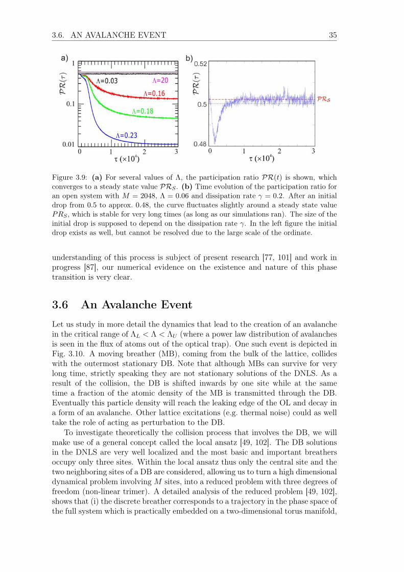
In the open system (γ > 0) the quantity PR = PR(t) is of course time de-pendent. After an initial drop, however, it rapidly approaches a constant valuePRS indicating a quasi-steady state (Fig. 3.9). In the following we study PRS asa function of the interaction strength Λ. Instead of a smooth transition betweenthe two extremes, as in the closed system, we observe a sharp drop of PRS at a


Figure 3.8: The localization parameter PRS vs. Λ≡λN(τ =0)/M is shown. For the closedsystem a smooth transition between the limits 1/2 and 5/9, which are given analytically,takes place. However, for the open system a sharp drop in PRS is observed, indicating aphase transition (see text).

critical interaction strength of Λb ≈ 0.15 as shown in Fig. 3.8, resembling a phasetransition. Our numerics indicate that this transition indeed becomes a step func-tion in the limit M → ∞. At Λb the order parameter PRS drops down to itslowest possible value (1/M) corresponding to a single occupied site, i.e. the finalstate consists of one single DB. We remark that for Λ < Λb, the atomic populationN(τ) decays smoothly to zero, following the same qualitative behavior as for theΛ = 0.

As we can see from Fig. 3.8, the transition between the linear regime and thecase where one DB is created becomes sharper in the thermodynamic limit. Thisindicates the existence of a phase transition. We have confirmed that the abovebehavior of the PR remains qualitatively the same for various values of γ rangingfrom 0.01 to 1. For Λ � 1, we recover the strong nonlinearity limit where manybreathers are found. However, we do not investigate the nature of the transition(e.g. if a similar ‘sharp’ transition takes place) in the strong nonlinear limit.

3.5.1 Nature of the Phase Transition

To understand the nature of the transition at Λb it is important to realize that ifa breather solution exists for some value of Λ, it exists for all Λ�s > 0 (for largeenough M). This can easily be seen by noting that a DB is not directly coupled tothe leaking edges, thus we can assume γ = 0 and then appropriately scale Eq. 3.5.Therefore breather solutions in particular do exist for Λ < Λb as well. For everynonlinearity Λ, however, there exists a lower bound for the norm carried by the DBs(that is well approximated by 1

2MΛ). For the dynamics to end in a single breatherstate the intermediate thermalized state therefore has to provide a fluctuation largeenough to create this breather, and at the same time all other fluctuations haveto be small enough not to destabilize the breather again. While a full (analytical)

3.6. AN AVALANCHE EVENT 35

Figure 3.9: (a) For several values of Λ, the participation ratio PR(t) is shown, whichconverges to a steady state value PRS . (b) Time evolution of the participation ratio foran open system with M = 2048, Λ = 0.06 and dissipation rate γ = 0.2. After an initialdrop from 0.5 to approx. 0.48, the curve fluctuates slightly around a steady state valuePRS , which is stable for very long times (as long as our simulations ran). The size of theinitial drop is supposed to depend on the dissipation rate γ. In the left figure the initialdrop exists as well, but cannot be resolved due to the large scale of the ordinate.

understanding of this process is subject of present research [77, 101] and work inprogress [87], our numerical evidence on the existence and nature of this phasetransition is very clear.

3.6 An Avalanche EventLet us study in more detail the dynamics that lead to the creation of an avalanchein the critical range of ΛL < Λ < ΛU (where a power law distribution of avalanchesis seen in the flux of atoms out of the optical trap). One such event is depicted inFig. 3.10. A moving breather (MB), coming from the bulk of the lattice, collideswith the outermost stationary DB. Note that although MBs can survive for verylong time, strictly speaking they are not stationary solutions of the DNLS. As aresult of the collision, the DB is shifted inwards by one site while at the sametime a fraction of the atomic density of the MB is transmitted through the DB.Eventually this particle density will reach the leaking edge of the OL and decay ina form of an avalanche. Other lattice excitations (e.g. thermal noise) could as welltake the role of acting as perturbation to the DB.

To investigate theoretically the collision process that involves the DB, we willmake use of a general concept called the local ansatz [49, 102]. The DB solutionsin the DNLS are very well localized and the most basic and important breathersoccupy only three sites. Within the local ansatz thus only the central site and thetwo neighboring sites of a DB are considered, allowing us to turn a high dimensionaldynamical problem involving M sites, into a reduced problem with three degrees offreedom (non-linear trimer). A detailed analysis of the reduced problem [49, 102],shows that (i) the discrete breather corresponds to a trajectory in the phase space ofthe full system which is practically embedded on a two-dimensional torus manifold,


Figure 3.10: Snapshot of an avalanche event. On the left subpanel, we are plotting τ

vs N(τ) whereas on the right we are reporting a representative collision event betweenthe outermost stationary DB and a moving DB (the color indicates the atomic densityNn(τ)). The moving breather of atomic density N

pert enters the monitored region fromthe right and collides with the stationary breather. During the collision, the stationarybreather gets destabilized and is shifted inwards while part of the moving DB ’tunnels’through the stationary breather and travels towards the edge of the lattice. The arrivalof the transmitted density at the edge is registered in the atomic population N(τ) as anavalanche event (see left subpanel). Note that for illustration, a representative avalancheevent in N(τ) is encircled in Fig. 3.4.

thus being quasiperiodic in time; (ii) the DB can be reproduced within a reduced(M = 3) system, called the nonlinear trimer.

3.7 Origin of the Scale-free AvalanchesEquipped with an understanding of an avalanche event, we now develop a physicalunderstanding on the origin of a power law distribution of the jumps through ananalysis of phase space structure of the reduced system: the nonlinear trimer [28].

3.7.1 Poincaré Section of the TrimerIn Fig. 3.11 we show a representative Poincaré section of the reduced system

for interaction strength Λ ≈ 1. The phase space consists of two components:islands of regular motion (tori) embedded in a chaotic sea. Trajectories insidethe islands correspond to DBs, provided that their frequency is outside the linearspectrum. In contrast, chaotic trajectories have continuous Fourier spectra, partsof which overlap with the linear spectrum of the infinite lattice [49]. Note that arepresentative Poincaré section of the nonlinear trimer including disorder (i.e. theon-site chemical potential µn is not constant in Eq. 3.4) exhibits as well a mixedphase space [103].

3.7. ORIGIN OF THE SCALE-FREE AVALANCHES 37

Figure 3.11: A Poincaré section of the phase space of the nonlinear trimer at Λ ≈ 1.0.Shown is N2 vs (φ3 − φ2)/π where φ’s are the angles in Eq. 3.2. The Poincaré section atΛ ≈ 1.0 corresponds to the plane φ1 = φ3 and φ1 > φ2 of the energy surface. It clearlyshows a hierarchical mixed phase space structure with islands of regular motion (tori)embedded in a sea of chaotic trajectories.

spert

Figure 3.12: Illustration of the arguments leading to Eq. 3.18. The figure shows an islandin a background of chaotic sea. Black ellipses correspond to regular orbits in an island,where s is the maximum diameter of the island. The blue ellipse is an example of aregular trajectory of a particle on the island, which corresponds to the case of a DB inour system. The destabilization of a stationary DB by a perturbation (e.g. a thermalfluctuation or a moving breather) with density N

pert ≡ Npert

1 is possible only if the DBcan be pushed out from the regular orbit across the island towards the chaotic sea. Theparticle’s motion then becomes chaotic, allowing for a continuous Fourier spectra andthus for dramatic increase of frequency overlap with the phonon band.


Figure 3.13: A destabilization process of a DB hosted by a closed trimer. We reportthe outgoing atomic population N

max

3 ≈ Nout (associated with an avalanche event – see

Fig. 3.10) measured at site 3 versus the incoming atomic population Npert

1 hosted bysite 1. We find that atomic population tunnels through the DB only if N

pert

1 � 0.25,corresponding to the minimal excitation needed to trigger the destabilization of the DB.Some of the density tunnels through the second site and reaches the third site. We registerthe maximum density on the third site as N

max

3 and obtain Nmax

3 ∝ Npert

1 . Analyticalexpressions for the minimal excitation necessary to destabilize the DB and an upperbound for the transmitted particle density N

max

3 are calculated in Sec. 3.8 and in [29].

The basic idea to explain the origin of the scale-free avalanches is the follow-ing: As long as the DB is stable, it acts as a barrier which prevents atoms fromreaching the leaking boundary. Thus, a necessary condition for an avalanche eventis the destabilization of the DB. As explained above, this can be caused by a lat-tice excitation (e.g. a moving breather) with particle density N

pert1 greater than a

threshold2. Due to the collision process, the regular or quasiperiodic orbit corre-sponding to the stationary breather can be pushed out of the island towards thechaotic sea, see illustration in Fig. 3.12. In other words, in order to destabilizea DB, one needs a perturbation that is at least of the order of the linear size s

(e.g. the maximum diameter) of the island which represents a DB. At the sametime a portion

J ≈ Nmax

3 ∝ Npert

1 ∝ s (3.18)

is transmitted through the DB (Fig. 3.13). Therefore, this destabilization processlets a fraction N

max

3 ≈ Nout of the perturbation tunnel through (see Fig. 3.10) which

reaches the leakage at the edge of the lattice, triggering an avalanche. Hence, thetask to understand the origin of the power law distribution of jumps P(J) translatesinto the study of the distribution of island sizes P(s).

2Strictly speaking, this is valid only for a fixed relative phase between the DB and the moving

breather as the destabilization holds for the total energy, as explained in Sec. 3.8 and in [29].


Figure 3.14: Illustration of the simple hierarchical model. This sketch shows the exampleof n = 3. The 0-th level main island has diameter s0 and is surrounded by n = 3 sub-islands of size s1, in a background of chaotic sea. Due to self-similarity, if we zoom intoone of the sub-islands, we would recover the self-similar structure of the islands but nowwith the main island being in the k = 1 level with s1 diameter, surrounded by anothern = 3 sub-subislands with diameter s2.

3.7.2 A Simple Hierarchical ModelThe above analysis in the frame of the local ansatz, allows us to turn the problemof the analysis of P(J) to the analysis of the distribution of island sizes P(s) of thereduced system with M = 3 in the Λ-regime where the phase space is mixed. Thatenables us to determine analytical lower and upper boundaries for α by consideringa heuristic model that mimics the hierarchical (‘island-over island’) structure of atypical mixed phase space in d dimensions. Beforehand, it should be said that wedon’t aim to consider a simple hierarchical model for high dimensional mixed phasespaces in general, but for dimension d = 2. However, from a mathematical pointof view, our simple heuristic model works in any dimension.

We assume in the heuristic model that at each hierarchy level k > 0 a mainisland of linear size sk−1 exists with a number nk of sub-islands (see Fig. 3.14 forillustration). As a measure of the linear size s of an island, e.g. the maximumdiameter can be taken. At the k−th hierarchy level, the fraction of sizes of themain island to sub-island is fk = Sk−1

Sk. Then s(k) reads

s(k) =s0�k

i=1 fi

(3.19)

and the total number of islands up to level k is given by

p(k) =k�

i=1

ni . (3.20)

Setting s0 = 1 and making the additional simplifications fk = f and nk = n foreach hierarchy level, we obtain

sk = f−k (3.21)


while the total number of islands pk reads

pk =k�

i=1

ni = nk. (3.22)

Hence, with k = − ln sk/ ln f from Eq. 3.21 the distribution of island sizes yields

P(s) = nk(s) = n

− ln s/ ln f = s−α

, (3.23)

with exponent α = ln n/ ln f .Furthermore, analytical bounds for α can be obtained, as the two following

limiting cases have to be fulfilled:

1. The total number of islands Nisland(s) must diverge for s → 0 due to theself-similar structure of the phase space, which leads to a lower bound for α.

2. The total d-dimensional phase space volume Vd(s) has to be finite, resultingin an upper bound for α.

Thus, for the total number of islands

Nisland(s) =

smax�

s

p(s�)ds� = s

−α+1 − s−α+1max

(3.24)

we require that lims→0 Nisland(s) = ∞ yielding α > 1. Secondly, for the total phasespace volume Vd(s) to be finite, the integral

Vd(s) =

smax�

s

(s�)dp(s�)ds

� = s−α+1+d − s

−α+1+d

max(3.25)

needs to converge in the limit s → 0. This requirement leads to an upper boundα < 1 + d. Hence, the bounds for the power law exponent α read 1 < α < 1 + d,where d is the dimension of the phase space.

To summarize, for a 2-dimensional mixed phase space our simple hierarchicalmodel yields the analytical restrictions for the power law exponent α of the distri-bution of island sizes

1<α<3 , (3.26)

in excellent agreement with our numerical findings (Eq. 3.16).

3.7.3 Test with Standard MapThe power law distribution Eq. 3.23 is surmised to be a generic feature of dynamicalsystems with a hierarchical mixed phase space in 2D, of which the Poincaré sectionof the trimer is an example. To get further confidence on our heuristic modeling,we aim to check numerically whether the sizes of islands of a typical Hamiltonianmixed phase space system are really well approximated by a power law distribution.To our knowledge the distribution of island sizes in a mixed phase space has not


Figure 3.15: Numerical estimation of the distribution of island sizes in a mixed phase spaceof the standard map for kicking strength K = 3.5. We plot f(s, C0)/s

2 = (pin,out(s) −C0)/s

2, which is a measure of the circumference of the islands vs. their width s. Clearly apower law distribution over more than three orders of magnitude is found, with exponentα = 1.4. The red rectangle in the inset marks the mixed phase space region underinvestigation (see Fig. 2.3b for consecutive enlargements).

yet been analyzed in literature, which at first came as a surprise. However, whenconsidering the complexity and the hierarchical structure of a typical mixed phasespace – see Fig. 2.3b for consecutive enlargements of a typical mixed phase space– it becomes clear, that calculating the distribution of island sizes is a challengeof its own, as for convincing evidence of the existence of a power law distribution,several orders of magnitudes of island sizes have to be resolved.

We will numerically approximate the distribution of island sizes in a paradig-matic model of mixed phase space dynamics: the standard map (see Sec. 2.2.1 foran introduction). We used kicking strength K = 3.5 for our analysis, hence, forillustration, we chose the same value of K in Fig. 2.3b. The idea for the numericalapproach will be sketched here, while the details are given in appendix B.

We consider a region R (see inset of Fig. 3.15) in the mixed phase space of thestandard map containing an island (with its daughter islands) originating from aperiod 1 resonance3. We start two trajectories at random initial conditions r andr + s within R separated by a distance s = |s|. We follow the trajectories up totime T and proclaim a trajectory to be inside an island if it has not left the regionR after a time T (which will become more and more accurate with increasing T ).The quantity we are going to study is pin,out(s), which is the probability that the firsttrajectory is inside an island and the second is not. This probes the circumferencesof the islands with less and less error (as the size of an island is overestimated withthis method) with increasing T .

Assuming a power law distribution of island sizes with exponent α, we find thatpin,out(s) can be written as (see Appendix B)

3For a period N resonance, we could do the same with the N-th iteration of the map.


pin,out(s) = C0 + C1s2−α (3.27)

with constants C0 and C1. The constant C0 is estimated by

σ(C0) = minC∈I

(σ(C)) , (3.28)

where σ(C) is the standard deviation resulting from a linear fit on a double loga-rithmic scale of the function

f(s, C) = pin,out(s)− C , (3.29)

and I ⊂ R is an appropriate interval. We checked that C0 changes smoothly withthe iteration time T of the standard map.

Figure 3.15 shows the numerical results for pin,out(s) for different maximal it-eration times T . As T increases, the curves fit better and better the form ofEq. 3.27. Thus, for the standard map with K = 3.5, we have estimated a powerlaw distribution of island sizes with an exponent α = 1.4.

In conclusion, our approximation to the distribution of island sizes clearly ex-hibits a power-law distribution over more than three orders of magnitude thusconfirming the validity of Eq. 3.23. Hence, our results provide numerical evidencethat the power law scaling is a generic feature of a typical mixed phase space.

3.8 Nonlinear Trimer

The destabilization of a DB due to a collision with a lattice excitation accompaniedby a shift of the DB (typically by one site) towards the perturbation which we sawin Fig. 3.10, has been observed in the past in various discrete nonlinear systems[28, 58, 61, 86, 104]. Clearly, the stability of DBs with respect to perturbations[61, 75, 105, 106] plays an important role during the collision process. We sawnumerically, that beyond a certain threshold the DB can get destabilized while afraction of the (atomic) density of the lattice excitation tunnels through the DB(Fig. 3.13).

In this Section, let us consider a discrete breather (DB) centered in the middleof a nonlinear trimer. We will analytically calculate the total energy thresholdof the nonlinear trimer in order to enable a perturbation at site 1 to trigger thedestabilization of a DB centered at site 2 [29]. Furthermore, we will determine anupper boundary for the maximum (atomic) density that is transmitted through theDB in the course of the collision.

3.8. NONLINEAR TRIMER 43

3.8.1 Equations of MotionOur starting point are the equations of motion of the nonlinear trimer. The DNLSwith M = 3 lattice sites reads (see Eq. 3.4)

i∂tψ1 = λ|ψ1|2ψ1 −1

2ψ2

i∂tψ2 = λ|ψ2|2ψ2 −1

2(ψ1 + ψ3)

i∂tψ3 = λ|ψ3|2ψ3 −1

2ψ2 , (3.30)

where the wave functions are normalized such that the total atomic populationreads N =

�M

n=1 |ψn|2 = 1. The normalization condition corresponds to Eq. 3.12,however, here we are dealing with a closed system where the total norm N isconserved. In order to find exact DB solutions in Eq. 3.30 for the symmetric caseψ1 = ψ3, we make the ansatz

ψn(t) = Aneiwt

, (3.31)

with Amplitude An and frequency w (the latter which is the same for all three sites).This ansatz together with the conservation of norm yields the set of equations

− wA1 = λA31 −

1

2A2

−wA2 = λA32 − A1

1 = 2A21 + A

22 . (3.32)

The equations below will be written in terms of the nonlinearity λ = 2U/T . Notethat the equations can be easily rewritten in terms of the effective interatomicinteraction per site Λ = λ/3 (see Eq. 3.6), e.g. to apply the results to extendedlattices.

3.8.2 Asymptotic SolutionsWhat are the symmetric (ψ1 = ψ3) DB solutions for a given nonlinearity λ? First,we calculate the norm N2 = A

22 at the central site from Eqs. 3.32 which yields

λ(N2) =

√2(2N2 − 1)�

N2(1−N2)(3N2 − 1). (3.33)

For λ < 5.04 only one symmetric breather solution exists, while for λ > 5.04 thereare several solutions (see Fig. 3.16). To gain further insight into the nature of thesymmetric breather solutions in the trimer, we will revisit Eqs. 3.32, which we turninto a quartic equation

x4 +

λ√2x

3 −√

2λx− 1 = 0 , (3.34)

whereA2 = cos(arctan(x)) =

sig(x)√1 + x2

. (3.35)


0 1/3 1/2 10

5

10

15

N2

λ

Figure 3.16: DB solutions for the symmetric case ψ1 = ψ3. The repulsive case is treatedexplicitly (λ > 0), however, Eq. 3.33 and the equations below hold as well for the attractivecase (as explained in Sec. 3.2). We see that for nonlinearity λ > 5.04 three symmetricbreather solutions exist with |ψ2|2 > 0, where the solution for large norm at the centralsite is termed a bright breather, see Eq. 3.37.

Expansion of the exact real solutions of Eq. 3.34 in λ for the limiting case λ → 0yields

x1 = 1 +λ

4√

2− 5

64λ

2 +O(λ3)

x2 = −1 +λ

4√

2+

5

64λ

2 +O(λ3) . (3.36)

At λ = 0 the solution �ψ = (ψ1, ψ2, ψ3) reads �ψ0(x1,x2) = (1/2,±1/

√2, 1/2). Expan-

sion around the limit λ →∞ leads to four real solutions

x1 = − 1√2

1

λ− 1

4√

2

1

λ3+O(λ−5)

x2 = − 1√2λ + 2

√21

λ+ 14

√2

1

λ3+O(λ−5)

x3 = −√

2− 3

2√

2

1

λ− 69

16√

2

1

λ2+O(λ−3)

x4 =√

2− 3

2√

2

1

λ+

69

16√

2

1

λ2+O(λ−3) . (3.37)

For infinite λ the solutions read

�ψ∞(x1) = (0, 1, 0)

�ψ∞(x2) = (

�1/2, 0,

�1/2)

�ψ∞(x3,x4) = (1/

√3,∓1/

√3, 1/

√3) , (3.38)

where the solution �ψ(x1) is called a bright breather, �ψ(x2) is called a dark breather(due to lack of norm at the central site) and �ψ(x3,x4) are phase-wise and antiphase-wise time-periodic localized solutions. In the following, the fixpoint corresponding


Figure 3.17: (a) PN energy landscape (lower part) (b) PN shell and (c) Contour plotof (a). The three minima of the lower bound to the dynamics correspond to the brightbreather solutions at the three sites. All plots are shown for nonlinearity λ = 3.

to the bright breather �ψ(x1) = (Afix

1 , Afix

2 , Afix

3 ) will be analyzed with respect toperturbations.

3.8.3 Peierls-Nabarro Energy LandscapeWe define the Peierls-Nabarro energy landscape as follows: It is obtained for agiven configuration of amplitudes An, by extremizing H with respect to the phasedifferences δφij = φi − φj. where ψn = An exp(iφn):

Hl

pn= min

δφij

(−H) ; Hu

pn= max

δφij

(−H) , (3.39)

where Hl

pnand H

u

pnare the lower and upper part of the PN landscape. The phase

differences extremizing the Hamiltonian

H =λ

2(A4

1 + A42 + A

43)− (A1A2 cos(φ1 − φ2) + A2A3 cos(φ2 − φ3)) (3.40)

are δφ12 = δφ23 = (0, π). The PN energy landscape reads

Hl,u

pn= −λ

2(A4

1 + A42 + A

43)∓ (A1 + A3)A2 (3.41)

which is, due to conservation of norm (A22 = 1 − A

21 − A

23), a function of two

amplitudes. In Fig. 3.17 the PN landscape is visualized for λ = 3. It exhibits


Figure 3.18: Dynamics on the PN landscape. (a, c, d) A contour plot of the lower PNenergy landscape H

lpn is shown for total energy Etot > Ethrs = −1.311, i.e. above the

rim. A projection of the orbit for times t = 0 . . . 35 onto the A1–A3 plane is over-plotted(black curve), where the arrows mark the position at time t = 0. The input values forthe initial condition defined by Eq. 3.43 are given in the figures. In all cases the DB isdestabilized and the largest part of the norm migrates to site 1. We see that the PNenergy landscape clearly restricts the dynamics in all cases. (a, b) The dynamics fora total energy just above the rim (Etot = −1.310) and corresponding amplitudes Ai(t)are shown. (c) Dynamics for larger total energy Etot = −1.282. (d) For the sametotal energy Etot = −1.310 as is (a) but a different initial phase difference δφ the samequalitative behavior is found.

three minima corresponding to the bright breather solutions which are separatedby saddle points (called ’rim’ in the following) located for λ → ∞ at Ai =

�1/2

for i = 1, 3. The energy threshold Ethrs at the rim (obtained from Eq. 3.40) reads

Ethrs =λ

4+

1

2+

1

4λ+O(λ−2) . (3.42)

In order to investigate whether and in which way the PN landscape influencesthe dynamics of a perturbed fixpoint solution and the transfer of norm through theDB to the other side, we will look at two quantities in the A1–A3 plane (plottedon top of each other in Fig. 3.18(a,c,d)): First, the projection of an orbit onto theA1–A3 plane of a perturbed DB and second, the contour plot of the PN landscape


Figure 3.19: Maximum norm A23 that is transferred from site 1 to site 3 while the DB

centered at site 2 migrates to site 1 as a function of the total energy Etot. In all cases weset the initial phase difference δφ23 = π and λ = 3. Note that with λ = 3 (i.e. Λ = 1)we reside in the critical regime where scale-free avalanches are found (see Eq. 3.14). Thevertical dashed line indicates the destabilization threshold Ethrs (e.g. a threshold fortargeted energy transfer, see Sec. 3.9).

Hl

pn, both at a given total energy Etot.4 We choose the following initial condition:

�ψ(t = 0) = (−(Afix

1 + δA)eiδφ , A2,−Afix

3 ) , (3.43)

where A2 = (1 − |ψ1|2 − |ψ3|2)1/2 is given by the conservation of norm. WithEq. 3.43 the PN landscape H

l

pnis determined by the two parameters δA and δφ. In

all cases we set λ = 3, which leads to the destabilization threshold Ethrs = −1.311according to Eq. 3.42.

Fig. 3.18 shows that the PN energy landscape rigorously restricts the orbitswhile the rim governs the destabilization process. Note that the larger Etot, thelarger is the size of the “bubble” (with the term bubble we denote the accessibleregion of the PN landscape for A1 > 1/

√2). In the limit λ → ∞ the DB in the

center of the trimer gets destabilized for A1 > 1/√

2. An upper limit to the normthat is transmitted to site 3 is given by max(A3)|A1>1/

√2 , which is the maximum

value of A3 inside the bubble. As we see from Fig. 3.18d, the migration of theDB followed by transfer of norm through the barrier is observed as well for otherinitial phase differences (shown is δφ12 = π/2). Moreover, we have checked thatthe mechanism itself is widely independent of the choice of parameters, i.e. it isfound for a whole range of λ, δφ12 and Etot.

In Fig. 3.19, the maximum Norm A23 that is transmitted through the DB as

a function of the total energy is shown for three initial phase differences δφ12 =0, π /4, π /2. The dashed vertical line at Etot = Ethrs = −1.311 marks the totalenergy at the rim and is identified with the destabilization threshold of the DB.

4The upper PN landscape Hupn may affect the dynamics as well, however, in terms of the

destabilization process it is sufficient to focus on the lower part Hlpn.


The maximum norm at side 3 is closely below the approximated upper boundsdetermined by the maximum possible value of A3 inside the bubble of H

l

pn, where

the dashed-dotted curve results from an analytical calculation in the limit for verylarge λ and the solid curve is a numerical calculation. Thus, we found an upperbound to the norm transferred through the DB.

To summarize, the threshold and the tunneling process during the collision of aDB with a lattice excitation (e.g. a moving breather) was described analytically bydefining the 2-dimensional Peierls-Nabarro energy landscape. The PN landscaperestricts the dynamics of the trimer and the accessible region of the phase space.This restriction of the dynamics becomes very pronounced at the destabilizationthreshold, which is identified with a rim in the PN landscape.5 The effect is de-scribed in a broad range of the nonlinearity λ of the system and for any phasedifference δφ12 between the DB and the MB.

3.9 Possible ApplicationsThe investigation of an individual avalanche in Fig. 3.10 triggered our analysis ofthe collision process of a DB and a moving breather. We observed a thresholdfor the total energy below which a DB acts as a dynamical barrier (a reflecting’wall’) while above the threshold the MB can destabilize the DB and part of the(atomic) density of the MB tunnels through the DB. This process could lead toseveral applications.

One possible application refers to atom lasers, in particular the findings maylead to interesting applications for blocking and filtering atom beams. It could bea powerful tool for controlling the transmission of matter waves in interferometryand quantum information processes [106].

In a similar way, our findings can be related to the field of optics, as the DNLS iscapable of describing wave motion in nonlinear optical waveguide arrays (where con-trolled boundary leakage can be achieved with suitable mirrors [2]). Note that thelongitudinal space dimension of the waveguides plays the role of the time variable inthe DNLS. Discrete breathers in such two-dimensional networks were investigatedin the past years both theoretically and experimentally [1–3, 54, 55, 74, 88–92]and can exhibit a rich variety of functional operations such as blocking, routing orlogic functions [4, 5] (see Fig. 3.20). Experimental evidence of the destabilizationprocess of the stationary DB (described above) should be observable in nonlinearwaveguide arrays and might lead to functional operations such as filtering opticalbeams.

Another field of conceivable applications refers to the analysis of the destabi-lization of a DB in the reduced system: The nonlinear trimer. Applications couldbe possible in terms of a molecular trimer, in particular in biophysics. “If ’dis-crete breathers’ is the answer, what is the question?” This is the title of an articlewritten by G. P. Tsironis [62] giving an overview on how DBs could play a role inbiophysics. Let us consider a DB as a bundle of highly (exponentially) localized en-

5Furthermore, it can be shown [29] that the destabilization threshold during the collision of the

two breathers can be linked to the Peierls-Nabarro barrier of a single DB (The Peierls-Nabarro

barrier is described in Sec. 2.4 and e.g. in [60, 61]).

3.10. CONCLUSIONS 49

Figure 3.20: Scheme of possible dynamics of discrete (moving) breathers in nonlinearwaveguide arrays that shows all-optical routing of on input signal beam to a specificoutput position [5]. The signal input beam (red) crosses the array with virtually nodiffraction. A control beam (blue) at about the second harmonic wavelength is used toproduce a third diffractionless output beam.

ergy for a moment, then it is conceivable that a DB could indeed mediate so calledtargeted energy transfer (TET) [107] – an example for TET could be the trans-port of energy obtained by the hydrolysis of ATP from a donor site D througha macromolecule (e.g. a motor protein) to an acceptor site A with virtually nodissipation. In the framework of the DNLS, Kopidakis et al. investigated TET be-tween discrete breathers of two weakly coupled random nonlinear systems. Thesesystems could represent two independent molecules, two linked parts of the samefolded macromolecule etc. In a real physical or biological system the D-A pair maybe interacting with additional degrees of freedom. Under appropriate conditions,irreversible targeting occurs with almost complete energy transfer. Hence, thethresholded transfer of energy through a discrete breather that has been describedin this chapter could possibly play a role as well in molecular systems, e.g. in thefield of biophysics or biomolecular engineering. However, Tsironis concludes:

”...we see that breathers could in principle act as able energy managers inbiomolecules; the real question of course is whether nature is actually using theirservices.”

3.10 ConclusionsIn conclusion, we have studied the dynamics of BECs in a leaking optical lattice inthe framework of the DNLS. In particular, we have observed scale-free avalanchesin the decay of the atomic population, and showed that the avalanche events arerelated to the existence of DBs inside the OL. We provided an explanation of theseevents using the scenario of a collision process involving a stationary DB and alattice excitation (e.g. a moving breather) where a threshold of the total energy


exists, beyond which the DB gets destabilized. The fact that for a certain rangeof (a rescaled) nonlinearity Λ ∼ O(1) a power law distribution P(J) ∼ J

−α ofavalanches is found, suggests the existence of a phase transition in the system.To this end, we proposed an order parameter PR which measures the relativenumber of sites that are occupied by DBs. We have linked the observed power lawdistribution of jumps to the hierarchical structure of a mixed phase space shown bythe reduced system – the closed nonlinear trimer. Furthermore, a thorough analysisof the PN energy landscape of the closed trimer yields an analytical expression ofthe minimal excitation necessary to destabilize the DB.

Outlook To better understand the nature of the observed phase transition (atnonlinearity Λ = Λb), it would be of high interest to find an (analytical) expressionfor Λb as described in Sec. 3.5.1. The transition is related to the formation of DBsin the discrete nonlinear system and is subject of recent research [77, 101] and workin progress [87].

Secondly, it would be very interesting to analyze the nonlinear trimer withdissipation (at the ends) with respect to the observed mechanism of destabilizationof a DB followed by a transfer of atoms/energy through the DB. For the closed(i.e. non-dissipative) trimer, the analysis can be found in Sec. 3.8. When dissipationis included in the analysis, a link to experimental systems (molecular trimer) mightbe possible. A promising approach could be the Holstein model (see e.g. [1] for adetailed description of the Holstein model).

Another system of interest consists of three nonlinear sites (allowing for thedestabilization and shift of the DB) embedded in a linear chain (see as well [106]) toenable the investigation of collisions of DBs with lattice excitations and to comparewith the results on the stability of DBs in the nonlinear trimer.

Chapter 4

Fractal Fluctuations

4.1 Mesoscopic Conductance FluctuationsWhile in Chap. 3 the transport properties of bosons in leaking optical latticesare described, here we focus on electronic transport in open mesoscopic systems.In mesoscopic systems conductance fluctuations are a sensitive probe of electrondynamics and chaotic phenomena. A prominent feature of electronic transport inmesoscopic systems is that the conductance as a function of an external parameter,e.g. a gate voltage or a magnetic field, shows reproducible fluctuations caused byquantum interference [14–16]. Typical examples of a chaotic mesoscopic system inwhich these universal conductance fluctuations were predicted and measured, arequantum billiards (Fig. 4.1) [15]. See Sec. 4.1.1 for an overview.

A prediction from semiclassical theory that inspired a number of both theoreti-cal and experimental works in the fields of mesoscopic systems and quantum chaoswas that in chaotic systems with a mixed phase space these fluctuations wouldresult in fractal conductance curves (as described in Sec. 4.1.3) [17, 18]. Such frac-tal conductance fluctuations (FCF) have since been confirmed in gold nanowiresand in mesoscopic semiconductor quantum dots in various experiments [19–23]. Inaddition, FCF have more recently been predicted to occur in strongly dynamicallylocalized [24] and in diffusive systems [25].

Motivated by puzzling experimental results showing a dependence of the frac-tal dimension on the coherence length, we studied the classical limit of transport

Figure 4.1: Electron micrograph of a ballistic semiconductor quantum dot resembling astadium billiard with 1 µm bar to show the scale. The picture is taken from ref. [15].Transport measurements by Marcus et. al. exhibit universal conductance fluctuations asa function of an applied perpendicular magnetic field (for moderate fields smaller than3T ) [15].

51

52 CHAPTER 4. FRACTAL FLUCTUATIONS

Figure 4.2: (a) Scheme of a 2DEG (figure taken from materi-alscience.uoregon.edu/taylor/science/taylor_lab.html). (b) Illustration of an electronbilliard. The illustration shows some analogy to a macroscopic billiard, however, it doesnot account for quantum effects.

through quantum dots also finding fractal fluctuations. This chapter will show, thatthe conductance of purely classical (i.e. incoherent) low-dimensional Hamiltoniansystems very fundamentally exhibits fractal fluctuations, as long as transport is atleast partially conducted by chaotic dynamics. The fractal dimension is determinedanalytically and it will be demonstrated, that the fractal dimension is governed byfundamental properties of chaotic dynamics. In addition, we predict that FCF arenot only observable in systems with a mixed phase space but in purely chaoticsystems [30]. Note that in this chapter, in order to determine the fractal dimensionof the graph of a function T (k), we used the variation method (and double checkedwith the Meakin method), i.e., we calculated N(∆k) = V (∆k, T (k))/(∆k)2, whereN(∆k) ∝ (∆k)−D for a fractal curve of dimension D, as described in Sec. 2.3.

4.1.1 Electron Billiards

What is a mesoscopic electron billiard? Imagine a two-dimensional electron gas(2DEG) in a semiconductor heterostructure, where electrons can flow freely in aplane, as shown in Fig. 4.2. When a negative voltage is applied to a metallicgate on top of the heterostructure, a depletion area forms inside the 2DEG fromwhich the electrons are repelled. By choice of the geometry of the metallic gates,a quantum dot (we will call it a cavity) can be designed in the plane of the 2DEG.Two or more small channels connect the cavity to outside leads in order to enableconductance measurements. Typically, the size of the mesoscopic cavity is around1 µm. If a single particle picture is valid (e.g. the electron correlation can beneglected) and if disorder or impurities are absent, then the transport is ballistic.Furthermore, if the cavity boundaries are clean and steep enough such that theelectrons can be considered to reflect specularly from the “walls”, the cavity iscalled a mesoscopic billiard, in analogy to macroscopic billiards. In contrast tomacroscopic electronic transport, where Ohm’s law is valid, quantum effects comeinto play, see [108] for an introduction. An important and well understood exampleis that the conductance through a mesoscopic ballistic cavity forming a chaoticbilliard shows reproducible universal fluctuations as an external parameter, e.g. amagnetic field applied perpendicular to the plane of the 2DEG, is varied [15].

4.1. MESOSCOPIC CONDUCTANCE FLUCTUATIONS 53

4.1.2 Universal Conductance FluctuationsUniversal conductance fluctuations (UCF), which initially were studied in disor-dered mesoscopic conductors, are reproducible fluctuations of the conductance (asa function of an external parameter such as the magnetic field or the energy) onthe order of 2e²/h and are a quantum effect. The size of the fluctuations is inde-pendent of specific system parameters or the average conductance, see Fig. 4.3 foran example. Where do UCF emerge from? In a disordered mesoscopic conductor– which is smaller than the phase coherence length of the charge carriers but largecompared to the average impurity spacing – the transmission is the result of theinterference of many different, multiply-scattered and complicated paths throughthe system. As these paths are typically very long compared to the wave lengthof the charge carriers, the accumulated phase θ along the paths changes basicallyrandomly when an external parameter such as the energy or the magnetic field isvaried. This results in a random interference pattern, i.e. reproducible fluctuationsin the conductance of a universal magnitude on the order of 2e²/h. For a review see[33] or [109]. The role of disorder in providing a distribution of random phases canas well be taken by chaos. Thus, ballistic mesoscopic cavities like quantum dots inhigh mobility two-dimensional electron gases that form chaotic billiards show thesame universal fluctuations [15, 110, 111]. While for disordered media the shapeof the conductor is typically not relevant, it plays an important role for billiards.Assuming chaotic dynamics in the billiard, characterized by an exponential decayof the classical staying probability P (t) ∝ exp(−γt), semiclassical arguments leadto UCF [112]. The classical decay rate is reflected in the autocorrelation function

C(∆E) =< g(E)g(E + ∆E) >E

and leads to a Lorentzian for small ∆E:

C(∆E) =C(0)

1 + (∆E

γ� )2. (4.1)

The Lorentzian shape was found experimentally in chaotic billiards [110]. InFig. 4.4 UCF are shown, which we generated numerically by means of a LorentzianC(∆E). Note that the conductance curve is smooth on small scales.

Figure 4.3: Measurement of UCF on a gold nanowire in the late 1980s at temperatureT ≈ 0.04 K (figure adapted from [14]). The fluctuations were reproducible after days ofmeasurement.


Figure 4.4: UCF, which are generated numerically by means of the autocorrelationfunction C(∆E) from Eq. 4.1 as a function of an external parameter (e.g. the en-ergy or a magnetic field) are shown. The conductance was calculated according tog(∆E) = F [

�S(f) exp(iθ)], where uniformly distributed random phases θ were added

to the power spectral density S(f) (which is the Fourier transform S(f) = F(C(∆E))according to the Wiener-Khinchin-Theorem). Adding random phases θ imitates the ba-sically random changes of the accumulated phases along the multiply scattered pathsthrough the system. The enlargement shows that the conductance curve becomes smoothon small scales.

4.1.3 Fractal Fluctuations: SemiclassicsWe have seen that the conductance through a mesoscopic cavity as a function ofan external parameter (e.g. a gate voltage or a magnetic field) shows reproduciblefluctuations caused by quantum interference. In the following, we will give a shortoverview into the semiclassical theory [17], that predicts fractal conductance fluc-tuations in chaotic systems where the underlying phase space is mixed. Note thatin an experiment, chaotic systems typically exhibit a mixed phase space e.g. dueto the influence of the magnetic field or due to a soft-wall potential (in contrast toideally specularly reflecting hard walls).

Where does the fractality emerge from? If the average of the phase gain θ

accumulated on the different paths traversing the system exists, the conductancecurves are smooth on parameter scales that correspond to a change of the averagephase gain on the order of and smaller than the wave length of the carriers as wehave seen in Fig. 4.4. In systems with mixed phase space, where chaotic and regularmotion coexist, the phase gain of trajectories traversing the system, however, istypically algebraically distributed

P (θ) ∝ θ−γ , where γ < 2 (4.2)

and no average phase gain exists (neglecting the finiteness of the coherence lengthand assuming the semiclassical limit �eff → 0; The transition to the quantummechanical regime, i.e. the role of the finite �eff , is discussed in [18]). Therefore,the conductance curve of such a system fluctuates on all parameter scales and formsa fractal. Ketzmerick has shown, that under these conditions the conductance curvepossesses the statistical properties of fractional Brownian motion [17]. The fractal


Figure 4.5: (a) A typical hierarchical mixed phase space structure of a 2D chaotic systemand (b) FCF are shown. The figure is taken from ref [17]. The Poincaré surface in (a)shows for the example of an antidot array the intersections of one chaotic and 6 regulartrajectories with the (y = 0, vy > 0) plane [113]. The conductance fluctuations shown in(b) are described by fractional Brownian motion (D = 1.4).

Figure 4.6: Resistance (i.e. inverse conductance) versus magnetic field for the open sta-dium billiard at a gate voltage of 21.9 V and at 50 mK. The 2DEG was 95 nm below thesurface. Fluctuations of the resistance on both large and small scales can be seen. Theinset shows a scanning electron micrographs of a device similar to the one that was used.Schematically, a single classical trajectory through the stadium is drawn. The figure isadapted from A. Sachrajda et. al. [19].


dimension D is connected to the exponent γ of the algebraic distribution of phasegains by

D = 2− γ

2. (4.3)

Due to the algebraic distribution of the phase gain P (θ), the autocorrelation func-tion exhibits a cusp

C(∆E) = C(0)− (∆E)γ, (4.4)

in contrast to the Lorentzian shape of the correlation function for UCF where thecorresponding conductance curve becomes smooth on small parameter scales. Thesemiclassical argument leading to the cusp was confirmed experimentally in a one-dimensional periodic array of potential wells [114]. An alternative to reasoning withthe average phase gain is to discuss the staying probability [17]. In a mixed phasespace, the staying probability P (t) decays algebraically (with the same exponentγ as for the distribution of the average phase gain) as chaotic trajectories in thevicinity of the islands can get caught for long times in a scale-free manner in thehierarchy of cantori [36, 37, 115] – see Sec. 2.2 for an introduction. (We alreadyencountered the self-similar hierarchy of islands in a mixed phase space in Sec. 3.7,where we investigate the stability of discrete breathers consisting of BECs in opticallattices.)

An example of experimental evidence for the fractal behavior of the conduc-tance is shown in Fig. 4.6. In that work the conductance through a stadium bil-liard with lithographic radius of 1.1 µm was measured as a function of an externalmagnetic field perpendicular to the plane of the billiard. The cavity was definedusing metallic gates on a high mobility AlGaAs/GaAs wafer. The high mobilitymaterial provides the required long phase coherence length. The device leads weremade especially wide (0.7 µm) in order to allow most trajectories to rapidly exitthe stadium, with the exception of those trajectories which were trapped near thehierarchical phase space structure at the boundary between regular and chaoticmotion. This feature and the high mobility made this a suitable device for theobservation of fractal conductance fluctuations and explains, why in earlier exper-iments on conductance fluctuations in ballistic microcavities [15] no fractals wereseen.

4.1.4 Experiments Beyond SemiclassicsDue to the quantum nature of the FCF it came as a surprise when recent exper-iments indicated that decoherence does not necessarily destroy the fractal natureof the conductance curve but may only change its fractal dimension [116, 117].Namely it was found that with decreasing coherence length the scaling region overwhich the fractal was observed did not shrink – as would be expected from thesemiclassical arguments –, but that the fractal dimension changed. The results ofthe experiment can be seen in Fig. 4.7. A decrease in temperature enlarges theelectron phase coherence length and is therefore expected to induce more quantummechanical conduction. In addition, a decrease in cavity size should increase theinfluence of coherent transport processes.

In other words, from bottom to top in Fig. 4.7, the transport is expected to bemore and more classical. However, still the conductance curve retains its fractality,


Figure 4.7: Schematics (not to scale) of the gate patterns (top row) together with theequivalent scanning electron micrographs (second row from top) for several billiards. Bot-tom: Magnetoconductance fluctuations measured for billiards e, f, and g (see trace labels).Billiards e, f, and g have mean free path 4.4 µm and the same geometry as b but aredifferent sizes. All billiard openings are 0.2 µm wide. The traces are offset verticallyfor clarity. From top to bottom the temperature is decreasing for the first four curves(4.2 K, 1.4 K, 0.48 K, 0.03 K) at constant cavity size 1.0 µm

2, while for the lower threecurves at constant temperature (0.03 K) the cavity size decreases from top to bottom(1.0 µm

2, 0.36 µm2, 0.16 µm

2). The last number in the right-hand brackets indicates thebox-counting dimension D. Figure taken from [116].

though the fractal dimension decreases. This finding is quantified in 4.8(right),which shows that with decreasing quantum lifetime of states the fractal dimensionof the curves decreases as well, however, a change of the fractal scaling range(e.g. between the point DB2 and DB3 in Fig. 4.8(left)) was not observed. Theseexperiments seem to partly contradict the semiclassical theory of fractal scalingand inspired our investigations shown in the next chapter.

4.1.5 Fractal Fluctuations: Classical Origin4.1.5.1 Numerical Evidence

As a starting point of our investigations and to connect it to the experimentswe numerically study the classical conductance through a rectangle (hard-wall)and a stadium billiard (soft-wall) as a function of a perpendicular magnetic fieldas shown in Fig. 4.9. (Throughout this chapter, we will study the transmission,which, in accordance with the Landauer theory of conductance, is proportional


Figure 4.8: (left) Box-counting analysis of magnetoconductance curves. The data (solidline) follow a straight line (dashed line) between the magnetic field scales DB2 and DB3while the gradient of the line gives the fractal dimension of the curve under investigation.The insets (a) and (b) are derivative plots of the data and (c) shows the individual datapoints (for clarity only every tenth point is plotted). (right) Lifetime of quantum statesτq (lower curve) and fractal dimension (upper curve) as a function of the temperature.The figures are taken from ref. [116].

to the conductance, see e.g. [108].) Note that not only the phase space of thestadium but also of the rectangle billiard is mixed in the presence of a perpendicularmagnetic field. In both cases, fractal analysis clearly reveals the fractal nature ofthe conductance curves. As the simulation is purely classical, the fractal scalingcannot be caused by interference effects.

4.1.5.2 Model: Open Standard Map

So what is the underlying mechanism for the fractality of the conductance curveand how can we understand its dimension? To study this mechanism in detail wewill, because of its numerical and conceptual advantages, analyze the transport inChirikov’s standard map [39, 118, 119] (see Sec. 2.2.1). This paradigmatic systemshows all the richness of Hamiltonian chaos. And since – as will become apparentbelow – our theory relies only on very fundamental properties of chaotic systems,it is a natural choice as a model system. The standard map is defined by

θ� = θ + p

�

p� = p + K sin θ

with momentum p, angle θ and the ’nonlinearity parameter’ K, which drives thedynamics from fully integrable (K = 0) to fully chaotic (K � 8). In between the


Figure 4.9: Classical Conductance g(B) through a stadium (left, geometry as in ref. [19])and square billiard (right, geometry as in ref. [116]) versus magnetic field B. Both fluc-tuating conductance curves are fractals, as is shown in the insets by the result of thebox-counting analysis (see text). Their respective dimensions are D ≈ 1.28 for the sta-dium and D ≈ 1.25 for the square billiard.

phase space is mixed. The standard map can be interpreted as the Poincaré surfaceof an autonomous conservative system of two degrees of freedom. As such the mapcan by viewed to directly correspond to the Poincaré map at the boundary of achaotic ballistic cavity, connecting it conceptually with the experimental system.We introduce absorbing boundary conditions (see e.g. ref. [120]), i.e. when p exceeds(drops below) a maximum (minimum) threshold value, the particle is transmitted(reflected) and leaves the cavity. As can be seen right from the definition of thestandard map, the envelope of the entryset (which is the phase space projection ofthe injection lead) is simply half a period of a sine function times K.A trajectory entering the system eventually contributes either to the total transmis-sion or reflection, and we mark the corresponding point in the entryset by a colorcode (transmission: red, reflection: blue) as shown in Fig. 4.10. Chaotic dynamics,through its fundamental property of stretching and folding in phase space, leads toa lobe structure (see Fig. 4.11 (bottom)), which is typical for chaotic systems andnot special to the standard map. The lobe structure is translated into transmis-sion by summing up the intersections of the transmission lobes along a horizontalline, see Fig. 4.11. A lobe of thickness w gives rise to a maximum contribution∆T ∝ w

β with β = 0.5. Variation of the external parameter K = 7.55 leads toa fractal transmission curve T (K) with D ≈ 1.25. Note that with K = 7.55 wereside in a regime near to the first fundamental accelerator mode which terminatesat K = 7.45. However, trajectories in tiny accelerator mode islands which stillmight exist, exit the phase space region quickly, and do not affect the long-timesurvival statistics, thus making the system effectively fully chaotic.

An analysis of the distribution of the widths w of lobes exhibits a power law

n(w) ∝ w−α

. (4.5)


Figure 4.10: Illustration of the absorbing boundaries (green horizontals), the transmissionand reflection areas of the standard map and the phase space projection of the injectionlead (entryset). The entryset is shown after two iterations of the standard map.

In the next chapter, we will analytically relate the power law exponent of lobewidths to the fractal dimension of the conductance curves.

4.1.5.3 Analytics: Fractal Dimension

How does the fractal dimension depend on the power law distribution of lobe-widthsand the curvature of the lobes? To this aim, we study a random sequence of curvesegments mimicking the intersection of consecutive lobes of widths w, distributedalgebraically with exponent α and curved like w

β. We define Xi :=�

i

j=1 wj and

T (X) = (−1)i(X −Xi)β : Xi < X ≤ Xi+1 . (4.6)

An example of this curve of “random lobes” with α = 1.9 and β = 12 is shown in

Fig. 4.12 (top). The box-counting analysis clearly reveals a fractal structure.We further simplify the problem by replacing the lobes by a sequence of stripes

of widths x with power law distribution n(x) ∝ xα. Dispensing with the sign of

the fluctuation, the transmission reads

T (X) = (Xi+1 −Xi)β)β : Xi < X ≤ Xi+1 . (4.7)

This yields histogrammatic transmission curves T (X) like the bottom curve ofFig. 4.12. As shown in the inset, the fractal dimension of the resulting transmissioncurve remains unchanged compared to the corresponding calculation with random


Figure 4.11: How lobes translate into fluctuations: In the lower row the entryset of thestandard map with absorbing boundary conditions at ±3π for K = 7.5 and K = 7.6resp. can be seen. The three pictures in the center row show the magnification of thecentral sections of the entryset for three different values of K = 7.5, 7.55 and 7.6. Thetransmission T (K) for K = 7.5 . . . 7.6 is shown in the top left picture. Note that a smallchange in K shifts the lobes vertically, but conserves the overall phase space structure, andthat the largest fluctuations are caused by intersection with the apex of lobes. Startingfrom K = 7.5, a large transmission lobe is cut by the horizontal line (see text), i.e. thetransmission increases with K. In the same way, e.g. the fluctuations of T (K) nearK = 7.55 can be understood. The box-counting analysis reveals a fractal structure (topright).


Figure 4.12: Transmission T (X) for lobes (red upper curve, shifted along the y-axis forclarity) and stripes (black lower curve) for one and the same random distribution withα = 1.9, β = 0.5. The inset shows the box-counting analysis for the upper (red triangles)and lower transmission curve (black squares). The regression line is drawn for the uppercurve, whose fractal dimension is 1.41.

lobes within the precision of the box-counting analysis. Thus, the measured fractaldimension of the curve does not change when considering stripes instead of lobesand also when neglecting the sign of each contribution, confirming the intuition,that the fractal dimension depends only on the relative scaling, i.e. α and β, butnot on the detailed form of the curve sections.

For these curves like the bottom one of Fig. 4.12 with α − β > 1, we can givean analytical expression for the fractal dimension and then estimate the fractaldimension of the transmission curve in the standard map. We apply the box-counting method, which we therefore review shortly (see Sec. 2.3 and ref. [42]for a more detailed introduction). In this approach the fractal curve lying in an−dimensional space is covered by a n−dimensional grid. Let the grid consist ofboxes of length scale s. The box-counting dimension is then given by

D = − lims→0

log N(s)

log(s), (4.8)

where N(s) is the number of non-empty boxes. For our problem, we divide N(s)into three contributions N(s) = na +nb +nc, as schematically drawn in Fig. 4.13A.The number na of vertically placed boxes (see mark (a)) covering contributionsfrom stripes of widths x > s, reads

na(s) ∝1

s

� ∞

s

p(x)xβdx ∝ s

−(α−β). (4.9)

Secondly, the number nb of horizontally placed boxes covering horizontal con-tributions of stripes of widths larger than s, see Fig. 4.13A(b), is given by

nb(s) =1

s

� ∞

s

p(x)xdx <1

s

� ∞

0

p(x)xdx. (4.10)


Figure 4.13: A. Schematic transmission according to Fig. 4.12 (bottom), covered withboxes of size s. There are three contributions marked (a-c). B. Total number Nint(w) =�∞w

n(w�)dw� of lobes (for the open standard map with |p| < 4π) of width larger than

w on a double logarithmic scale. The four curves show estimates for increasing res-olution wmin = 10−5(pink) . . . 10−8(black). The curves clearly approach a power lawcorresponding to n(w) ∝ w

−1.9. The insets show the transmission curve T (K) for valuesK = 8.0 . . . 8.1 calculated from 2× 1013 trajectories and its fractal dimension.


Figure 4.14: Fractal dimension of transmission curves based on random lobes accordingto Eq. 4.12. In the legend, α is given, while β varies from 0.1, 0.2, . . . , 0.6, e.g. the threedata points around D = 1.4 correspond to (α,β ) = (1.7, 0.3), (1.6, 0.2) and (1.5, 0.1). ForD � 1.2 the data points lie on plateaus confirming the analytical relation D = α−β. Thesame results within the accuracy of the fractal analysis are obtained when calculating thetransmission according to Eq. 4.7. The error bars in the figure are an estimate and areof total size 0.025.

Hence nb scales like s−1 and can be neglected in comparison to na because of

α−β > 1. Finally, we determine an upper estimate for the number nc of verticallyplaced boxes covering the contribution from stripes of widths x ≤ s. The totallength of these widths is L(s) =

�s

0 p(x)xdx, therefor L(s)/s boxes are needed tocover the length. Inflating all heights of the stripes x ≤ s to the maximum possiblesize s

β, see Fig. 4.13A(c), we find

nc(s) <L(s)

s

sβ

s∝ s

−α+β. (4.11)

For s� 1 thus the dominant terms is na(s). With Eq. 4.8, N(s) gives rise to thebox-counting dimension

D = − lims→0

log s−α+β

log s= α− β. (4.12)

A numerical calculation of the fractal dimension of transmission curves based onrandom lobes for various pairs of (α,β ) shows good agreement with the analyticalresult for α− β � 1.2, as can be seen in Fig. 4.14.

To connect the analytical result with the calculations of the transmission ofthe open standard map, we numerically estimate the distribution of lobe-widthsin the entryset as shown in Fig. 4.13B for K = 8, where we obtain α ≈ 1.9.Together with β = 1/2, corresponding to first order Taylor expansion of the cosinefunction, Eq. 4.12 predicts a fractal dimension D ≈ 1.4. Direct analysis of thetransmission curve (see insets of Fig. 4.13B) yields a fractal dimension D ≈ 1.39,in good agreement with the expected value.


4.1.5.4 Origin of the Power Law

How can a power law distribution of lobe widths emerge in a fully chaotic opensystem? Rather one might have expected to find an exponential distribution oflobes in a fully chaotic system. To see why the distribution is algebraic, however, letus examine the simplest case of an open chaotic area preserving map the dynamicsof which is governed by a single, positive homogeneous Lyapunov exponent λ. Ineach iteration phase space structures are stretched in one direction by exp(λ),shrunk by exp(−λ) in the other and then folded back. The entryset of the opensystem is thus stretched into lobes of decaying width w(ti) ∝ exp(−λti). Thephase space volume flux out of the system decays exponentially as it is typical fora fully chaotic phase space, i.e. Γ(ti) ∝ exp(−ti/τ), with (mean) dwelltime τ . Thearea Γ(ti)∆t is the fraction of the exitset that leaves the system at time ti. Withti(w) ∝ − ln(w)/λ the number of lobes of width w in the exitset is

N (w) ∝ Γ(ti(w))∆t

w∝ 1

wexp(

ln(w)

λτ) = w

1λτ−1

.

This suggests that the power law distribution of lobe widths is a generic propertyeven for fully chaotic systems. A quantitative expression for the exponent, however,is not as easy to derive, as e.g. the Lyapunov exponent for the standard map isnot homogeneous. Note that we showed the argument for the exitset and not forthe entryset for the sake of clarity. A corresponding relation for the algebraicdistribution of lobe widths in the entryset can be derived easily by studying thetime-reversed map, which again is a chaotic map with the same properties.

4.1.6 ConclusionsWe have shown that the conductance of purely classical (i.e. incoherent) low-dimensional Hamiltonian systems very fundamentally exhibits fractal fluctuations,as long as transport is at least partially conducted by chaotic dynamics. Thusmixed phase space systems and fully chaotic systems alike generally show FCF.More specifically, we have shown that transport through chaotic systems due tothe typical lobe structure of the phase space in general produces fractal conductancecurves, where the fractal dimension reflects the algebraic distribution of widths oflobes P (w) ∼ w

−α in the exit- /entryset. We showed analytically that under theseconditions the fractal dimension reads D = α− 1/2.

To connect with the semiclassical picture of FCF, note that an implicit assump-tion of the semiclassical theory is that the classical dynamics remains unchangedas the external parameter is varied and thus only phase changes are relevant. Inmany experimental setups, however, the external parameter is changed consider-ably, leading to very noticeable changes in the classical dynamics. Moreover, wehave shown that the classical chaotic dynamics itself already leads to fractal con-ductance curves! From this follows that even on very small parameter scales thefluctuations due to changes in the classical dynamics are important. In contrastto the semiclassical effect the size of the fluctuations is not universal but dependson specific system parameters. Due to the fractal nature of the classical conduc-tance, however, there is no parameter scale that separates coherent and incoherentfluctuations.


In conclusion we are led to the following scenario: In general the conductancecurve of low-dimensional Hamiltonian systems is a superposition of two fractals –one originating in interference which is suppressed by decoherence to reveal thefractal fluctuations reflecting the changes in the classical phase space structure.

4.2. LONG-RANGE CORRELATIONS IN MUSIC RHYTHMS 67

4.2 Long-range Correlations in Music RhythmsA completely different system where fractal fluctuations are found, is musicalrhythm played by humans. While in the case of fractal conductance fluctuations,we are interested in the structures on smaller and smaller scales, here the long-time correlations lead to the fractal nature of the fluctuations. Still, the idea ofinvestigating human rhythms emerged from studying FCF.

Music rhythms performed by humans will always exhibit a certain amount offluctuation compared with an exact rhythm (e.g. given by the steady beat of ametronome). We refer to these fluctuations as temporal deviations which denotethe occurrence of individual sounds slightly before or after the exact point in time(see Eq. 4.13). It is believed that the task of synchronizing the movement of one’sfinger to a periodic environmental signal (finger tapping) shows deviations from thesignal which exhibit long-range correlations (1/fβ-type) [121–124]. But musiciansdo not restrict themselves to finger tapping. Are long-range correlations (LRC) incomplex music rhythms played by humans generic?

Long-range correlations (1/fβ-type) are ubiquitously found in various scientificdisciplines, examples include DNA sequences [125], condensed matter [126, 127],econophysics [128], human coordination [129, 130], astronomy [131, 132], neuro-physics (see e.g. [133, 134] and references therein), etc. General concepts [36, 100,135] aim at explaining the omnipresence of 1/fβ noise in nature.

Specifically, one encounters 1/fβ noise in heartbeat intervals [45, 136–138] andin loudness and in pitch fluctuations in music and speech [26, 27, 139]. The pitchfluctuations were measured by the rate of zero crossings of the audio signal, which,in terms of music, approximately follows the melody. 1/fβ noise in both loudnessand pitch fluctuations was used for stochastic composition which was judged bymost listeners to be more pleasing than that obtained using white noise or 1/f2

noise [26, 27].In this section, we show that the temporal fluctuations in simple as well as in

more complex music rhythms are generic in the sense that Gaussian 1/fβ noise isproduced, no matter if the task is accomplished with a finger, a hand, a stick, afoot, a combination of these or the voice [31]. The exponent β, however, dependson the individual and on the specific task. We found a variety of exponents in therange 0.2 < β < 1.3. In other words, we are dealing with fractional Gaussian noisein the time domain of human music rhythms, which is of stochastic nature and,in contrast to conductance fluctuations in mesoscopic systems, not reproducible.The fluctuations that we focus on comprise of generic (natural) deviations from agiven rhythmic pattern – in contrast to intentional accentuations. Accentuationfacilitates the interpretation of a music piece and thus plays an important role;however, this is not treated here.

The fact that long-memory processes arise in a broad variety of complex rhyth-mic tasks suggests that a common basic neurophysical mechanism accounts forgeneric creation of human rhythms. It is most likely that 1/fβ noise in musicrhythms is not generated in the course of the movement of a limb but due to aneuronal network that is responsible for perception and estimation of time. See[140–142] for an overview on neurophysical modeling of rhythmic timing and esti-mation of time intervals in the millisecond regime. We will briefly review an idea


e1e2 e3

tS2 S3M2 M3M1 S1

Figure 4.15: Schematic plot of a rhythmic music sequence (e.g. a drum sequence) and ametronome, only pertaining to the temporal occurrence of sounds. The drum sequencewith beats at times Sn is compared to the metronome Mn yielding errors en = Sn −Mn.

based on a simple stochastic model [143] which generates pulse trains exhibiting1/fβ noise in Sec. 4.2.3.

Moreover, in Sec. 4.2.4 we are led to an application of our findings by addressingthe following question: Does the rhythmic structure of a piece of music soundbetter when it is as exact as possible or are ’natural’ deviations (comprising long-range correlations) in music rhythms more favorable? Professional audio softwareapplications include a so called ’humanizing’ feature, which adds deviations en (alsoreferred to as errors, see Eq. 4.13) to a given audio sequence. Hence, there existsa desire to generate or modify music on a machine that sounds more natural. Weanalyzed the humanize tool of such contemporary software applications and foundthat e.g. for the program ’Pro Tools’1 it consists of Gaussian white noise. So howdoes a music piece humanized with Gaussian 1/fβ noise sound? We show withsimple computer-generated drum rhythms, that the 1/fβ humanized music (withβ ≈ 1) was rated significantly better by professional musicians from the GöttingenSymphonic Orchestra than the conventional humanized sequences comprising aGaussian white noise error source with the same standard deviation. However, thesimple drum rhythms used in the experiments sound rather artificial and the exactrhythm was preferred over the humanized versions.

For more realistic experiments on the influence of LRC in music rhythms onthe perception of humans, a music piece (more specifically a pop song) was cre-ated, recorded and humanized in cooperation with Cubeaudio recording studio(Göttingen). Experiments with test subjects were carried out in the course of aninterdisciplinary diploma thesis in psychology [32] (see Sec. 4.2.4.3). Applicationsare possible in humanizing music sequences with Gaussian 1/fβ noise, e.g. in thefield of electronic music or in post-production of real recordings, where a patent inthe EU and the USA was applied for (Sec. 4.2.4.4).

4.2.1 Error Time SeriesIn this section, we will make the basic definitions needed and give an illustrativeexample of the error time series originating from a recording of human rhythmicdrumming.

1Pro Tools is widely used by professionals throughout the audio industries worldwide for

recording and editing in music production, film scoring, post production etc.


Figure 4.16: Recording beats on a drum. A subject, here a professional drummer, isplaying on a drum. The sounds are recorded with a microphone at sampling rate 44.1khz. Photo taken from www.hippocritz.com by courtesy of Agbenyega Attiogbe.

A simple way to define the deviations of human drumming from a rhythmicreference pattern is to take a metronome as a reference (see Fig. 4.15). Given a’metronome’ Mn = M0+nT , where T denotes the time interval between metronomeclicks and n = 0, 1, 2 . . . is an integer. And given a (recorded) rhythmic musicsequence with sounds (also referred to as beats) at times Sn, then the error timeseries is defined as

en = Sn −Mn , (4.13)

where en � T ∀n. A sound is given by the audio signal A(t) (e.g. the voltage inputto a loudspeaker) and as such is extended in time. We define the occurrence of asound at time Sn by

A(Sn) = max(A(t)) , (4.14)

which is well-defined in particular in drum recordings (Fig. 4.16) due to the compactshape of a drum sound A(t): The envelope of A(t) rises to a maximum value (“attackphase”) and then decays quickly (“decay phase”) [144]. Thus, if the drum soundsare well separated, a unique maximum A(Sn) can be found. In contemporaryaudio editing software, typically the onset of a beat is detected [144, 145], whichis very useful when beats overlap or when dealing with distorted sequences. InSec. 4.2.4.2 we will use onset detection to find the temporal occurrences of soundsfor humanizing music sequences.

The definition Eq. 4.13 can be easily generalized to considering deviations ofa sequence from a complex rhythmic pattern instead of from a metronome. Thetime between two successive sounds τi = Si+1 − Si (also called interbeat intervals)is connected to the timing errors by

τi = T + ei+1 − ei . (4.15)

In the following let us define the terms 1/fβ noise and long-range correlations.Given a discrete stochastic process x(t), customarily, one speaks of 1/fβ noise,


whenS(f) = |F(x(t))|2 ∝ f

−β and 0 < β < 2 , (4.16)

where F denotes the Fourier transform. Note that there are as well definitionswhere 0 < β < 1, see e.g. [146]. In literature, both notations 1/f and 1/fβ

noise are found for the same entity. For simplicity, from now on we will drop theexponent and speak of 1/f noise meaning 1/fβ noise with 0 < β < 2. For β = 0the time series x(t) is uncorrelated (white noise), while for β = 2 it corresponds toBrownian motion (integrated white noise). In addition, when the x(t) are Gaussiandistributed, it is called Gaussian 1/f noise (also referred to as fractional Gaussiannoise).

A (discrete) long-memory process is defined as a stochastic process where theautocorrelation function C(k) =< x(t)x(t+k) > corresponding to a time series x(t)decays to zero so slowly that it is not summable (in the discrete case) [121, 146]:

∞�

k=0

C(k) = ∞ , (4.17)

which holds, ifC(k) ∝ k

−γ and 0 < γ < 1 , (4.18)

also referred to as long-range correlations (LRC). Finally, for 0 < γ < 1, Eqs. 4.16and 4.17 are connected by the Wiener Khinchin theorem

S(f) = F(C(k)) (4.19)

where S(f) ∝ fγ−1 for a long-memory processes.

A simple example of a recording and its processing is shown in Figs. 4.16 and4.17: Here, the given task was to follow the clicks of a metronome given overheadphones with a hand on a drum at 180 beats per minute (bpm). The output isrecorded with a microphone. A comparison of Sn with the metronome (Eq. 4.13)leads to the error time series en. As we see from Fig. 4.17b, en fluctuates arounda mean of −16.4 ms. In other words, the negative value means that the subjectanticipates the next metronome click.

In Fig. 4.18 the power spectral density S(f) = |F(en)|2 of our example isshown. The frequency range under consideration is fmin < f < fnyquist/2, wherefnyquist = 0.5 sec−1 is the Nyquist frequency (i.e. half the sampling frequency of theerror time series). The corresponding time window reads Tmin < T < Tmax, whereTmin = (fnyquist/2)−1 60/180 = 1.3 sec and Tmax = 333 sec. A least squares fit of thePSD in the considered frequency range indicates that S(f) can be approximatedby a power law

S(f) ∝ f−β (4.20)

with exponent β ≈ 1.2. However, to closely investigate the long-range behavior ofthe time series, we used several methods described in Sec. 4.2.2.

4.2.2 Data Set & AnalysisThe data set analyzed in Fig. 4.21 consists of the recorded output of several rhyth-mic tasks performed by humans, which can be divided into three subsets Sdrum,Ssing


Figure 4.17: (a) The drummer in Fig. 4.16 was recorded in tapping with the hand onthe drumhead of a drum according to the clicks of a metronome, that were given overheadphones. Shown is a section of the recorded amplitudes (e.g. the voltage input signalto a loudspeaker) over the beat index n. A beat-finder detects the temporal occurrence ofthe beats (green lines), here given by the maximum of the amplitudes. The metronome(red dashed lines) has 180 bpm, i.e. two consecutive clicks are separated by 1/3 sec.(b) Corresponding error time series of the recording. The errors e284 to e288 depictedin Fig. 4.17a are marked with red squares. Note that values en < 0 indicate that thesounds occur earlier than the metronome click. Inset: The pdf of the time series is wellapproximated by a Gaussian distribution in agreement with a previous analysis of fingertapping data [121]. The Gaussian distribution in this example has mean −16.4 ms andstandard deviation 15.6 ms.


0.001 0.01 0.1 0.510−5

10−3

10−1

101

frequency f

S(f)

∼ f−1.2

Figure 4.18: Power spectral density (PSD) of the time series in Fig. 4.17. Note thatthis figure serves only as an illustration – for clear statistical estimates several methodsfrom time series analysis are applied in Sec. 4.2.2. The PSD indicates 1/f

β noise at lowfrequencies in the range fmin < f < 0.25 = fnyquist/2 with β ≈ 1.2. Note that thelogarithmic transform does not preserve the structure in the variance of the estimatesat each frequency. Estimates at frequencies with high amplitudes have lower relativevariances than the relative variances at frequencies with low amplitudes. Since in 1/f

noise, low frequency is associated with high amplitudes, this produces the triangularstructure, where the bottom part of the envelope descends more steeply than the toppart. An averaged PSD of the same time series analyzed here is shown in Fig. 4.19b(second curve from top).

and Stap. All subsets have in common that a human was given metronome clicksover headphones. To address the task that was recorded, leading to an error timeseries e

In, we annotate each error time series with a task index I, which denotes

the specific task explained in the following (e.g. I = (1, 2) corresponds to tasks 1and 2 in Fig. 4.21).

The subset Sdrum consists of drum recordings provided by a recording studio2

and of recordings that we made. During professional drum recordings in a studio,a drummer is sitting in front of a drum set and uses both arms and the feet togenerate a complex music rhythm that, typically, is part of a piece of music. Thefeet are used for operating pedals connected to bass drum and hi-hat (Fig. 4.23).During a studio recording it is customary, that the drummer hears metronomeclicks over headphones while playing. We make use of this fact to analyze the errortime series of professional drumming data. Given the speed of the song, usuallymeasured in beats per minute (BPM), a comparison of the drum recordings withthe metronome can be drawn. In detail, the subset Sdrum comprises error timeseries e

In

obtained from several recordings of different tasks I = (1− 7):

• e(1,2)n : Studio data of 2 drummers belonging to different music bands playing

different patterns at 190 bpm and 132 bpm. The drum sequences analyzedeach are part of a music song.

• e(3−5)n : Short rhythmic pattern at 124 bpm. The pattern (given in 4/4 bars)

2Cubeaudio Recording Studio, Göttingen, Germany


contains quarter and eighth notes, is of 2 bars length and is repeated contin-uously by the drummer.

• e(6,7)n : Tapping with a drum stick on a drum according to the clicks of the

metronome at 124 bpm.

More specifically, e(3−5)n originate from the same recording, but the time series e

(3)n is

obtained by comparison with a 248 bpm metre (thus focusing on the deviations inthe eighth notes), while e

(4)n is obtained by comparing the beats with respect to the

metronome at 124 bpm. In e(5)n the off-beats are analyzed (i.e. by comparison with

a metronome at 124 bpm that is shifted by T/2). To summarize, the complexity ofthe rhythmic patterns in the subset Sdrum decreases from e

(1,2)n over e

(3−5)n to e

(6,7)n .

At the one end there are real drum recordings that are part of popular music songs,while at the other end a link to finger tapping analyzed in literature [121–124] ismade.

Secondly, the subset Ssing consists of 4 recordings (I = (8 − 11)) of shortrhythmic sounds of the voice according to a metronome at 124 bpm. We chose shortphonemes (such as [’dee’]) to obtain well-peaked amplitudes of the beats. However,the fact that long-range correlations are found is expected to be independent of thephoneme that is articulated.

Finally, the subset Stap comprises of tapping experiments (I = (12−27)) similarto what can be found in literature, but to connect with the subset Sdrum we recordedtapping with a finger or a hand on the drumhead of a drum. We recorded tappingat two different metres for each test subject: 124 bpm (even task index) and 180bpm (odd task index)3. We discarded the first 50 beats to eliminate transients.When a deviation is larger than 100 ms, than that beat is called a ’glitch’ and isomitted, which happened in less than 5 out of 1000 cases for the recordings in Ssing

and Stap and does not appear to affect the long term behavior we seek to quantify.Test subjects in Stap and Ssing were of mean age 33± 9 yrs.

We used several methods to analyze the correlation properties of the data,namely the periodogram (also referred to as PSD), detrended fluctuations analy-sis (DFA), and the maximum likelihood estimation (MLE [147], details are givenbelow). See Sec. 2.3.1 for a short introduction to fractal analysis.

For the estimate via the periodogram, a least square fit of the power spectraldensity S(f) = |F(en)|2 is made on a double logarithmic scale.4 As the variance ofthe PSD is large (at high frequencies), an average of the PSD is taken (Fig. 4.19).For the averaging, the time series is divided into boxes of length L, and in eachbox the arithmetic average is taken. We used L = 5 and checked that moderateaveraging L ≤ 10 does not notably alter the resulting exponent.

The second method, DFA, is applied directly in the time domain, see Sec. 2.3.1and [45, 149] for details. The integrated time series is divided into boxes of equallength s. DFA involves a detrending of the data in the boxes using a polynomialof degree k. Then the sum F (s) of the fluctuations over the trend is calculated.

3Only exception are tasks 14 and 15 which both are recordings at 124 bpm.4A comparison of the linear regression with a band integrated regression, where the points in

the power spectrum are equidistant, shows that the linear regression leads to more reliable results

[148].


Figure 4.19: Examples of the averaged PSD of different error time series of the data set.The red straight lines are least square fits in the regime fmin < f < fnyquist/2, thusindicating a long-range behavior of the correlations. (a) Analysis of different complexdrum sequences. The upper two curves originate from the analysis of drum sequences oftwo different songs provided by a recording studio. For the lower two curves we maderecordings of a drummer continuously repeating a drum pattern. (b) Examples from thePSD of Ssing and Stap. The upper two curves show the PSD for tapping on a drum for twodifferent professional drummers. The lower two curves show the analysis of recordings ofshort rhythmic sounds of the voice according to a metronome. Subjects were a professionaldrummer and a professional a-capella singer.

Again, a linear relationship on a log-log plot indicates the presence of power law(fractal) scaling F (s) ∼ s

α. The scaling exponent α is related to the PSD exponentβ by [146]

β = 2α− 1 . (4.21)

In case of fractional Gaussian noise α = H is the Hurst exponent. We calculatedthe DFA exponents using DFA2, which means quadratic detrending (k = 2), seeFig. 4.20. Similar results were obtained with linear detrending (DFA1).

Once it is statistically established by means of PSD and DFA that the spectraldensity S(f) is well-approximated by a power law, we use the MLE to estimate theexponent β and determine confidence intervals. The MLE is applied to S(f) in thesame frequency range as for the PSD method (i.e. fmin < f < fnyquist/2 = 0.25).

Results

As can be seen in the examples in Figs. 4.19 and 4.20 (task index for top to bottomcurves are I = (2, 1, 3, 5) and I = (22, 21, 8, 10) in Fig. 4.19a and Fig. 4.19b) thetime series exhibit long-range correlations. We find Gaussian 1/f noise for thewhole data set; see Fig. 4.21 where the exponents β with corresponding confidenceintervals are collected. We emphasize that the exponent β of the Gaussian 1/f noiseis not universal and varies in our data set between 0.2 < β < 1.3. Note that the ex-


101 102101

103

105

box size s

F(s)

∼ s0.66

∼ s0.64

∼ s1.04

∼ s0.73⇒ β =0.5

⇒ β =1.1

⇒ β =0.3

⇒ β =0.3

Figure 4.20: Examples of detrended fluctuation analysis (DFA2) for the same error timeseries analyzed in 4.19b, i.e. the lower two curves correspond to recordings of short rhyth-mic sounds of the voice, while the upper two curves originate from tapping on a drum.Clearly, a fractal scaling F (s) ∼ s

α is found for box sizes in the range 6 < s < N/4, whereN is the total length of the time series. To compare with the exponents β calculated inFig. 4.19b, the PSD exponents β = 2α− 1 are given as well.

Figure 4.21: Results of the time series analysis of the whole data set obtained fromdifferent rhythmic tasks. The tasks correspond to (complex) drum sequences (I = (1−7)),rhythmic vocal sounds (I = (8 − 11)) and to tapping with a finger or hand on thedrumhead of a drum (I = (12 − 27)) . All sequences recorded lead to error time seriesthat exhibit Gaussian 1/f noise. The exponents β obtained by the different methodsPSD, DFA2 and MLE are compared and show overall good agreement. The confidenceintervals are provided by the MLE. The two tasks in-between two neighboring verticaldashed lines are recordings of the same test subject at different metronome tempi (124bpm and 180 bpm respectively), e.g. tasks 20 and 21 are recordings of the same individual.


ponent varies as well within recordings of different tasks made by the same person.For example for the tasks I = (8, 20, 21) the same person was recorded (who is aprofessional drummer), where the different MLE exponents β(I) = (0.4, 0.7, 1.1)are obtained.

The tasks in the whole data set are quite diverse and the data set is not largeenough to significantly detect task-dependent differences. However, our focus willbe on generic long-range correlations in music rhythms that appear in all tasks andwith every subject that we recorded (as long as the subject was able to follow therhythm).

Is the exponent related to the music expertise of the person recorded? In thesubsets Ssing and Stap we recorded musicians and non-musicians with different mu-sical experience ranging from laypersons to professionals, where the music expertisewas estimated by a self-evaluation. In the subset Sdrum the subjects recorded aredrummers, i.e. experienced in playing the drums. A clear dependence between β

and the music expertise was not found in the data set. A prerequisite for LRC isthat the person is able to follow the rhythm. Long-range correlations vanish, if theindividual loses the rhythm too often and reenters with help of the metronome –we speculate that this resets the memory of the internal mechanism (some kind of“dynamical clock”, see Sec. 4.2.3) responsible for the rhythmic timing.

Another considerable quantity is the standard deviation of the error time series(the average for the whole data set is σ = 21 ms). The lowest standard devi-ations were found for musicians, however a musician does not necessarily intendto minimize the standard deviation. We surmise that the more a person tries tosynchronize with the external metronome, which can reduce the standard devia-tion in case of trained drummers to σ < 10 ms, the lower the exponent β. Thissuggests that some sense of rhythmic timing is crucial for LRC, where the degree ofthe correlation shrinks with increasing external influence. In the limit, where thetest subject is triggered completely externally (as in reaction time experiments),no LRC are found [122].

We are led to the following conjecture: When a musician is strongly triggeredexternally (by a metronome or another music sequence) and synchronizes highlywith the external signal, the degree of long-range correlations in the correspondingerror time series is smaller than in the case when the musician is ’free floating’,i.e. triggered mostly internally.

4.2.3 Modeling Rhythmic DrummingIt seems most likely that 1/f noise in music rhythms is not generated in the courseof the movement of a limb but due to a neuronal network that is responsible forperception and estimation of time. An overview on neurophysical modeling ofrhythmic timing and estimation of time intervals in the millisecond regime is foundin [140–142, 150]. As described in [140], modeling an internal clock that couldaccount for timing in the millisecond regime has been a challenge for decades, seee.g. [124, 151] for recent approaches. The millisecond regime is defined in [140]as being above 10 ms and below 500 to 1000 ms. Since experienced drummersachieve standard deviations of below 10 ms, we alter the time scale of interest forour purposes to 5 < T < 500 ms. The human reaction time lies within that regime:


Figure 4.22: Dynamics of a single neuron model which exhibits long range correlated (1/f

type) pulse trains [143]. The model is based on an integrate-and-fire mechanism consistingof two variables: A linearly increasing potential V (t) and a threshold C(t) which evolvesaccording to a random walk with diffusion constant D and reflecting boundaries. Whenthe potential V (t) exceeds the threshold, a spike is generated and V (t) is reset. However,the interspike intervals can be approximated by a 1 dimensional map with multiplicativenoise (Eq. 4.22), which does not show long range correlations in the τk.

For the tasks where subjects depress the space bar on a computer keyboard asrapidly as possible after the presentation of an optical stimulus the reaction timehas mean ∼100 ms [122].

A simple stochastic model for which it can be shown analytically to generatespike trains exhibiting 1/f noise is presented by Davidsen and Schuster [143]. Theessential ingredient of the integrate-and-fire model is a fluctuating threshold whichperforms a Brownian motion. Whenever an increasing potential V (t) hits thethreshold, V (t) is reset to the origin and a pulse is emitted (Fig. 4.22). If V (t)increases linearly in time, the interspike intervals (ISI) τk can be approximated bya random walk with multiplicative noise [143]:

τk+1 = τk +�

Dτk ξk , (4.22)

where ξk denotes the white noise source and D is the diffusion constant. However,there are drawbacks when relating Eq. 4.22 to the interbeat intervals Eq. 4.15. ThePSD of the above-mentioned spike trains (which can be idealized to a sequence ofzeros and ones, where a 1 indicates the occurrence of a spike) reveals a long-memory process. In contrast, it can be shown that a time series τk (Eq. 4.22) doesnot exhibit long-range correlations. A second problem is, that for the random walkwith multiplicative noise, the ISI distribution function P (τ) is proportional to τ

−1

[143], while the pdf of the interbeat intervals in human rhythmic drumming is wellapproximated by a Gaussian distribution.

In order to develop some further aspects of Davidsen’s and Schuster’s model,several approaches are possible. One approach is to adaptively change the gradienta of the linearly rising potential of the neuron, trying to keep a mean ISI τ . Thisintroduces a second parameter a where the ISI τk depend on a. Another idea isrelated to synchronization, or simply to coincidence. For our purposes, consider N

neurons described by the single neuron model (Fig. 4.22) which are connected to


one neuron A, which integrates the incoming spikes of the N neurons and whichsends an action potential, if the following condition is fulfilled: M out of N presy-naptic neurons fire in the same time window. Note that it was shown in purelyrandom networks, that synchronous spiking activity of subgroups can persist andpropagate if the non-additive nature of dendritic input integration has been re-cently uncovered experimentally is taken into account [152]. We surmise that thecondition (i.e. the requirement of coincidence of M/N spikes) for neuron A to spikealters the distribution of the ISI such that it is different from a power law and mayapproximate a Gaussian. However, the modeling is still work in progress.

4.2.4 Humanizing Music Sequences

As shown in Sec. 4.2.2, we found 1/f noise in the error time series of music rhythmsplayed by humans. In this section, we will consider an application arising from thequestion, which effect long-range correlations have on the perception of humans.

Computer-generated music, such as an artificial drum sequence, has no difficultyin always keeping the exact beat, since synthesizers and computers are equippedwith precise timing mechanisms. But computer-generated music is often recogniz-able just for this perfection. The idea to artificially add small fluctuations to musicsequences is realized in the so-called ’humanizing’ feature, which is implementedin contemporary audio software applications. More precisely, humanizing is theprocedure of adding an error time series en (Eq. 4.13) to a given audio sequence.We analyzed the humanize feature which leads to error time series consisting ofGaussian white noise for the program ’Pro Tools’ (Version HD 7.4) and of uniformwhite noise for ’Nuendo 3’. Pro Tools is widely used by professionals throughoutthe audio industries worldwide for recording and editing in music production, filmscoring, post production etc. In terms of humanizing music, we are led to thequestion:

• How does a piece of music humanized with Gaussian 1/f noise sound incomparison to a piece of music that is either conventionally humanized orexact?

• Are the differences audible to humans?

To investigate these questions, different pieces of music were created and playedto test subjects as described in the next sections. For each piece of music threeversions were generated which differ only by their error time series en (Eq. 4.13):

1. Version E (’exact’): en = 0∀n.

2. Version C (’correlated’): Ce(τ) =< en, en+τ >= τ1−β with exponent β ≈ 1

(thus exhibiting long-range correlations). Also referred to as the Gaussian1/f humanized version.

3. Version W (’white’): en = ξn, where ξn is Gaussian white noise. Also referredto as the Gaussian white noise humanized version.


Figure 4.23: Scheme of a drum set with bass drum (4), snare drum (5) and hi-hat (6).Samples of bass drum, snare and hi-hat were used to generate humanized drum rhythms.

All other properties of the versions (such as the pitch and loudness fluctuationswhich do affect the auditory impression [26, 27, 139]) are identical. To comparethe versions E, C and W, we choose the same standard deviations σC = σW of theerror time series and mean < eE >=< eC >=< eW >= 0.

The outline of the following sections is as follows. In Sec. 4.2.4.1 the generationof simple humanized drum rhythms is described and we report the rating of thedifferent versions by test subjects. The creation of a much more complex humanizedpiece of music is explained in Sec. 4.2.4.2. The rating of the piece of music by testpersons is subject of an interdisciplinary diploma thesis in psychology (Sec. 4.2.4.3).Finally, in Sec. 4.2.4.4 a patent for humanizing music sequences is described.

4.2.4.1 Drum Rhythms

We generated simple drum rhythms on the computer, where each drum rhythmconsists of 3 different audio samples (bass drum, snare drum, hi-hat – see Fig. 4.23)that are set according to a rhythmic pattern. An audio sample of e.g. a bass drumis a recording of a single bass drum sound. The exact sequence is then humanizedto generate versions C and W by adding a 1/f or white noise error time series (seeFig. 4.24). Though this is a first demonstration of 1/f humanizing of electronicmusic, the minimalist way of the generating the music rhythms with only 3 samplesmakes the rhythmic pieces sound quite monotonous and artificial. Furthermore themusic sequences do not contain any variation in timbre of the beats, in loudness orpitch.

For statistical tests, the different versions E, C and W of the drum sequences,each in mono quality and of ≈ 30 sec length, were played in random order (thereare subtleties, see Appendix C) to 16 professional musicians from the GöttingenSymphonic Orchestra (GSO). The test subjects completed a questionnaire, themain questions are shown in Fig. 4.25. For the experiments with the GSO we useda standard deviation σC = σW = 10 ms. Audio examples (no. 1, 2 and 3) of theversions E, C and W with σC = σW = 15 ms are found as supplementary materialto the electronic version of this thesis. To make the differences between the versionsmore audible, the standard deviation in the audio examples is higher than in theexperiments. Still, σ = 15 ms is within the lower range of σ measured for musiclaypersons while finger tapping on a drum (with a finger or a hand). We used aχ

2-test with significance level p0 = 0.05, see Appendix C for details. The outcome


0.5 1 1.5

−0.5

0

0.5

1

1.5

time / sec

ampl

itude

Asnare+Ahi−hat

e4 e6

Abass+Ahi−hat

e2

Ahi−hat0.2 sec 0.2 sec0.4 sec

Figure 4.24: How (1/f) humanizing works. Shown is a section of an exact drum sequence(lower curve) with 153.6 bpm at 4/4 bars and a humanized sequence (upper curve). Thelength of one quarter note is 0.4 sec. The lower and upper sequences correspond to thefirst ≈ 1.5 sec of audio examples no. 1 and 2 respectively. For 1/f humanizing the uppersequence, to each individual sound at time Sn an error en is added, where en is computer-generated Gaussian 1/f noise with β ≈ 1. The vertical dashed lines mark the positionsSn of the sounds.

Figure 4.25: The main questions of the questionnaire given to musicians from the Göttin-gen Symphonic Orchestra. We did not analyze the third question (which version soundsmore natural / more precise), as all versions sound rather artificial, due to the minimalistconstruction of the drum rhythms with 3 samples.


E vs. W C vs. W E vs. C0

20

40

60

80

100

comparison of versions

ratin

g in

%

92%92% 83%

Figure 4.26: “Which version sounds better?” Experiments with 16 musicians from theGöttingen Symphonic orchestra rating the 1/f humanized version C the white noisehumanized version W and the exact version E. Two versions were played after one another(in random order), 10 comparisons were made by each test subject. Version C was ratedsignificantly better than version W (p = 0.02, χ

2 = 5.3) with 83 % vote. A preferencewas given to the exact version, compared to both the versions C (p = 0.002, χ

2 = 9.3)and W (p = 0.002, χ

2 = 9.3).

of the experiment with the GSO is the following (Fig. 4.26):

• The 1/f humanized versions are rated significantly better than the (conven-tional) white noise humanized versions (p = 0.02, χ

2 = 5.3).

• The exact version was rated best (p = 0.002, χ2 = 9.3).

One reason why the exact version is preferred may be due to the artificial characterof the rhythmic sequences. Thus, deviations are perceived as failures by the testsubjects. The fluctuations in the rhythmic structure might be rated differentlywhen more complex artificial music or music originating from real recordings (thatinclude as well fluctuations in timbre and loudness) is humanized. Though theexact version was rated best, a comment of one of the test subjects from the GSOsummarizes our idea of a perceived lack of human touch nicely:

Some samples were so ’overprecise’, too regular by intention – that does not soundnatural.

4.2.4.2 Creating Humanized Music

In order to compare the version C, W and E in a more realistic way, a pop songcalled “Everyday, everynight” was created, recorded and humanized in collaborationwith Cubeaudio recording studio (Göttingen). The song has 125 bpm, approx. 4mins length and a steady beat in the eighth notes. Hence, the song consists of ∼1000 beats in the eighth notes. Instrumentation was chosen such that the sequencescan be humanized easily, meaning that the sounds occurring at times Sn should berather compact and well separated from each other.The song, available in stereo quality, consists of a total of ∼100 sequences includingseveral sequences for the drum set (as the output of each part of the drum set,


e.g. the bass drum, was recorded individually), guitar, bass, vocals and, to a smallpart, software instruments. Except for the software instruments, the sequences arerecordings of professional musicians, where each musician is recorded separately. Inthe next step, the individual sequences are humanized and finally mixed together.The program ’Pro Tools’ was used for onset detection [144, 145] of the beats andfor mixing the song. Note that the complexity of the song (consisting of mostlyreal recordings of several instruments, and including fluctuations of loudness andpitch in ∼ 100 sequences) is much higher than that of the single drum sequencesgenerated with the computer as described in Sec. 4.2.4.1.

We did not humanize the vocals, which cover the fluctuations of the otherinstruments to a certain degree. The vocals are identical in all three versions E,C and W. To generate version W, we did not use the white noise humanize toolimplemented in Pro Tools, but we added the white noise error time series manuallyto have control over the realizations and the standard deviation.

The version C was humanized with 1/fβ noise, where β ≈ 1. The standarddeviations of the versions C and W is σ = 15 ms, which is a trade-off betweenhaving significant results (for large σ) and a regular (natural) sound (for small σ).The Gaussian was cut at 2σ, i.e. realizations larger than 2σ were omitted in thetime series, in order to exclude single rare events that might influence or dominatethe judgment of listeners.

Still, there is a main drawback, that give the song an artificial touch. Wehumanized all ∼ 100 sequences with one and the same error time series (1/f orwhite noise).5 This leads to collective shifts (or delays) in the time domain, whichis not natural, as all instruments come in too early or too late at a given time inexactly the same manner.

4.2.4.3 Perception of Humanized Music

How does a piece of music humanized with Gaussian 1/f noise sound in compar-ison to a piece of music that is either white noise humanized or exact? The aimof the interdisciplinary diploma thesis in psychology that we initiated was to ana-lyze the perception of natural fluctuations in music rhythms using the humanizedsong “Everyday, everynight”. The thesis is written by Anneke Fredebohm at theUniversity of Göttingen (Dept. of Cognitive and Decision Sciences). More specifi-cally, a comparison of the two versions C and E is drawn, where audio examples oflength ≈ 30 sec were played in random order (there are subtleties, see [32] for theexperimental design) to 57 listeners who are mostly part of non-professional choirsin Göttingen. There was no information given in advance to the subjects, in whichway the versions differ. The differences between the three versions E and C arevery small and, moreover, they are covered by the vocals. It can be shown using aχ

2-test that [32]

• the test subjects could significantly hear the difference between the versionsE and C (p = 0.015),

5The reason why we used the same time series for humanizing all sequences is because 1/f

humanizing is not yet implemented in contemporary audio software applications and thus had to

be done manually and double-checked afterwards.


• there was no preference found when comparing versions E and C.

Note that there is a distinct difference to the simple and artificial drum rhythmsanalyzed in Sec. 4.2.4.1, where a clear preference for the exact version was observed.Hence the rating of the 1/f humanized piece of music (as compared to the exactsequence) was much better than in the case of the less complex drum sequences.The versions, that the test subjects were listening to are found in audio exampleno. 4 : First, the version C and after a 5 sec break the exact version E is played.

A comparison of the versions C and W is current work in progress (see audioexample no. 5, which consists of the version W, a 5 sec break and the version C).We expect a preference of version C over version W, which would mean that inagreement with the previous study described in Sec. 4.2.4.1, rhythms containingLRC are preferred over those containing white noise error time series.

Surprisingly, as stated above, the version containing LRC was not rated betterthan the exact version. There are several reasons, which could account for that.First, the standard deviation of σ = 15 ms is too large for a popular song (espe-cially if the listeners are experienced musicians). Second, all sequences were (asmentioned above) humanized according the same realization of the error time se-ries, leading to unnatural collective shifts of all instruments (except for the vocals).And third, it is probably a matter of individual taste and may depend on the musicgenre [139], whether a song or parts of the sequences within should be as exact aspossible of whether natural deviations are tolerated and favored. The complete1/f humanized song with reduced standard deviation σ = 7.5 ms, correspondingto quite precisely playing musicians, is attached to the electronic version of thisthesis (audio example no. 6).

We made a first step towards the realization of 1/f humanizing of music se-quences. To what extent 1/f humanizing will be useful for audio engineers remainsto be seen in practice when it is applied in a more sophisticated way to sequencesin music pieces.

4.2.4.4 Patent

The Max Planck Society applied for patents in the EU and the USA for humaniz-ing music sequences with error time series consisting of 1/f noise. The title of theapplication reads: “Method and Device for Humanizing Music Sequences” (EU ap-plication no: 07117541.8 (Sept. 2007), US application no: 12/236,708 (Sept. 2008)).A short extract of the application, that was filed in collaboration with Max-Planck-Innovation, is given below.

“The present invention relates to a method and a device for humanizing musicsequences. In particular, it relates to humanizing drum sequences. Large partsof existing music are characterized by a sequence of stressed and unstressed beats(often called "strong" and "weak"). Beats divide the time axis of a piece of musicor a musical sequence by impulses or pulses. The beat is intimately tied to themeter of the music as it designates that level of the meter that is particularlyimportant, e.g. for the perceived tempo of the music. A well-known instrumentfor determining the beat of a musical sequence is a metronome. A metronome isany device that produces a regulated audible and/or visual pulse, usually used to


establish a steady beat, or tempo, measured in beats per minute for the performanceof musical compositions. Ideally, the pulses are equidistant. However, humansperforming music will never exactly match the beat given by a metronome. Instead,music performed by humans will always exhibit a certain amount of fluctuationscompared with the steady beat of a metronome.

Machine-generated music on the other hand, such as an artificial drum sequence,has no difficulty in always keeping the exact beat, as synthesizers and computers areequipped with ultra precise clocking mechanisms. But machine-generated music, anartificial drum sequence in particular, is often recognizable just for this perfectionand frequently devalued by audiences due to a perceived lack of human touch.The same holds true for music performed by humans which is recorded and thenundergoes some kind of analog or digital editing. Postprocessing is a standardprocedure in contemporary music production, e.g. for the purpose of enhancinghuman performed music having shortcomings due to a lack of performing skills orinadequate instruments, etc. Here also, even music originally performed by humansmay acquire an undesired artificial touch.

Therefore, there exists a desire to generate or modify music on a machine thatsounds more natural. It is therefore an object of the present invention to providea method and a device for generating or modifying music sequences having a morehuman touch. Preliminary results of empirical experiments carried out by theinventors strongly indicate that a rhythm comprising a natural random fluctuationas generated according to the invention sounds much better or more natural topeople than the same rhythm comprising a fluctuation due to Gaussian or uniformlydistributed white noise with the same standard deviation.”

4.2.5 ConclusionsWhen a human plays a music rhythm on an instrument, inherently there are devi-ations in the time domain from the exact rhythm. We showed that music rhythmsperformed by humans generically exhibit long-range correlations in the deviationsfrom an exact rhythmic pattern. The deviations are generic in the sense, that thecorresponding time series can be described by Gaussian 1/fβ noise, no matter if themusic rhythm is made with a finger, a hand, a stick, a foot, a combination of theseor the voice. The exponent β is not universal and depends on the task and thesubject. Moreover we investigated the influence of long-range correlations in musicrhythms on the perception of humans. We showed that music when it is humanizedwith Gaussian 1/fβ noise is rated significantly better by listeners than the samesequences humanized with Gaussian white noise. We expect that in principle, aftersubtraction of accentuation, rhythmic long-range correlations exist when humansplay on many different kinds of instruments, examples include musicians singing orplaying the guitar or the piano.

Outlook It would be interesting to further develop a neurophysical model thataccounts for time estimation on the time scale of milliseconds, where a startingpoint could be Davidsen’s and Schuster’s model [143]. Another open question is,in which way the correlation properties of the error time series change when two(or more) musicians play together. A simplified problem is, how the temporal


correlations in a music rhythm played by a human are influenced by a metronome,which contains fluctuations around the exact metre.

Chapter 5

Conclusions and Outlook

In conclusion we have studied transport phenomena, scale-free properties and frac-tal fluctuations in different complex dynamical systems. This thesis was presentedin two main parts.

In the first part (Chap. 3), we have studied the dynamics of BECs in leakingoptical lattices in the framework of the DNLS. We investigated the flux of ultracoldatoms out of the optical trap and hence analyzed the survival probability N(τ)which decays in sudden jumps J = δN for a certain range of the nonlinearityΛ. We found that these jumps, also referred to as avalanches, follow a scale-freedistribution

P(J = δN) ∼ 1/Jα.

The avalanche events are accompanied by the formation of discrete breathers insidethe optical lattice for a nonlinearity Λ > Λb. Our numerical findings indicate theexistence of a phase transition at Λb. To this end, we proposed an order parameterwhich measures the relative number of sites that are occupied by the BEC. Wehave linked the observed power law distribution of jumps to the distribution ofisland sizes in the mixed phase space of the reduced system: the closed nonlineartrimer. Using the standard map as a paradigmatic model for mixed phase spacedynamics, we provided evidence that a power law distribution of island sizes is ageneric feature of the mixed phase space. In a simple model that imitates the self-similar hierarchical structure of the mixed phase space we found analytical boundsfor the exponent yielding 1 < α < 3 in agreement with our numerical findings.

We explained the avalanche events using the scenario of a collision processinvolving a stationary DB and a lattice excitation (e.g. a moving breather) wherea threshold exists, beyond which the DB gets destabilized. The destabilization of aDB due to the collision leads to a shift of the DB towards the perturbation. Duringthe migration process, a fraction of the (atomic) density of the excitation ’tunnels’through the DB leaving the system as an avalanche. We showed that there exists atotal energy threshold in the trimer, in order to enable a perturbation at site, say,1 to trigger the destabilization of the DB at site 2. The destabilization threshold isdescribed analytically by considering the dynamically accessible region of the phasespace and linked to the Peierls-Nabarro barrier of a single DB. Furthermore, anupper boundary for the (atomic) density that tunnels through the DB to site 3 isgiven analytically. The existence of the destabilization threshold could be used as

86

87

a tool for controlling the transmission of coherent atomic beams in interferometryand quantum information processes.

The DNLS can be applied to a variety of physical systems, a prominent exam-ple are coupled nonlinear optical waveguide arrays. In this context, avalanches ofBECs translate into the scale-free statistics of light emittance from waveguide ar-rays. Discrete breathers in such two-dimensional networks were investigated in thepast years both theoretically and experimentally and can exhibit a rich variety offunctional operations such as blocking, routing or logic functions [4, 5]. Experimen-tal evidence of the destabilization process of the stationary DB is expected to beobservable in nonlinear waveguide arrays and might lead to functional operationssuch as filtering optical beams.

In the second part (Sec. 4.1) we analyzed the ballistic flux of electrons throughmesoscopic systems such as quantum dots, nanowires and electron billiards. Moti-vated by unexpected experimental findings on fractal conductance fluctuations inelectron billiards, where the fractal dimension changed with the coherence length,we simulated purely classically the conductance through electron billiards with dif-ferent geometries and found clear numerical evidence for FCF of classical origin.We have shown using standard map, that transport through chaotic Hamiltoniansystems in general produces fractal conductance curves, where the fractal dimen-sion reflects the distribution of lobe widths P (w) ∼ w

−α in the entry-/exitset whichis the phase space projection of the leads attached to the conductor. We empha-size, that chaotic dynamics, through its fundamental property of stretching andfolding in phase space, leads to such a lobe structure, which is typical for chaoticsystems and not special to the standard map. An analytical estimation of thefractal dimension yields D = α− 1/2.

To investigate the origin of the power law distribution of the lobe widths, weexamined the simplest case of an open chaotic area preserving map the dynamicsof which is governed by a single, positive homogeneous Lyapunov exponent λ. Weshowed that under these conditions the number of lobes of width w in the entrysetreads

P (w) ∝ w1

λτ−1,

with mean dwelltime τ . This suggests that the power law distribution of lobewidths is a generic property even for fully chaotic systems.

It is known that the semiclassical theory leads to fractal conductance curvesdue to interference of the numerous electron paths. To connect our results with thesemiclassical picture of FCF, note that an implicit assumption of the semiclassicaltheory is that the classical dynamics remains unchanged as the external parameteris varied and thus only phase changes are relevant. Here it was shown that the clas-sical chaotic dynamics itself already leads to fractal conductance curves, i.e. evenchanges of the classical dynamics on arbitrary small scales lead to fluctuations ofthe conductance. Due to the fractal nature of the classical conductance, there isno parameter scale that separates coherent and incoherent fluctuations.

In conclusion we are led to the following scenario: In general the conductancecurve of low-dimensional Hamiltonian systems is a superposition of two fractals –one originating in interference which is suppressed by decoherence to reveal the

88 CHAPTER 5. CONCLUSIONS AND OUTLOOK

fractal fluctuations reflecting the classical phase space structure. This might ex-plain the unexpected results of experiments in semiconductor quantum dots wherea dependence of the fractal dimension on the coherence length was observed. Fur-thermore, we predict fractal fluctuations in the conductance of low-dimensionalHamiltonian systems with a purely chaotic phase space.

In Sec. 4.2 we considered temporal fluctuations in music rhythms played byhumans yielding long-range correlations. We showed by analyzing a set of differ-ent rhythmic tasks, that the temporal fluctuations in simple as well as in morecomplex music rhythms generically exhibit Gaussian 1/fβ noise. A range of expo-nents 0.2<β< 1.3, depending on the individual and the task recorded, was found.The fact that long-memory processes arise in a broad variety of complex rhythmictasks strongly supports the hypothesis, that a common basic neurophysical mech-anism accounts for interval timing in the millisecond regime (see [140, 141] for anoverview). We shortly reviewed an idea based on a simple stochastic model [143]that generates spike trains exhibiting long-range correlations (1/fβ-type), which iswork in progress.

Using humanized music, we showed that the 1/fβ humanized versions (withβ ≈ 1) were rated significantly better by listeners than the conventional human-ized sequences comprising a Gaussian white noise error source. Applications arepossible in humanizing music sequences with Gaussian 1/fβ noise, e.g. in the fieldof electronic music or in post-production of real recordings. To this end, a patentin the EU and the USA was filed by the Max Planck Society, termed “Method anddevice for humanizing music sequences”.

As an outlook on future works on the DNLS with leaking boundaries (“avalanchesof BECs”), it would be fascinating to see the experimental verification of the pre-dicted avalanche statistics. Second, even though we do have clear numerical evi-dence for the phase transition, which is related to the formation of DBs in the opendiscrete nonlinear system, the origin of the phase transition together with an ana-lytical expression for Λb is still an open and fascinating question (see [28, 77, 101])and work in progress [87].

As far as the study on the closed nonlinear trimer and the observed mecha-nism of destabilization of a DB is concerned (Sec. 3.8), a natural next step is theanalysis of the nonlinear trimer including dissipation. This may provide a betterdescription of the transfer of atoms/energy through the DB and a link the resultsto experimental systems (e.g. a molecular trimer) might be possible. A promisingtheoretical approach could be the Holstein model. Another system of interest con-sists of three nonlinear sites embedded in a linear chain (see as well [106]) to enableinvestigations of collisions of DBs with linear lattice excitations.

On the outlook on FCF, it would be of high interest to study the transition fromthe semiclassical to the classical limit where experimentally a smooth change of thefractal dimension was observed. So far, rigorous theoretical descriptions exist onlyfor the two limiting cases, i.e. in the classical case (analyzed as part of this thesis)and in the semiclassical limit [17, 19].

We hope that we contributed a small part in solving the puzzles emerging fromscale-free fluctuations in complex systems.

Appendix A

Limiting Cases of the Participation

Ratio

We will calculate the participation ratio (Eq. 3.17)

PR(τ) =

�[N(τ)]2

M�

n|ψn(τ)|4

�

(which is a measure of the relative number of sites occupied by atoms in the leakingOL) for the closed system (i.e. γ = 0) in the two limiting cases Λ � 1 and Λ = 0.

(a) Λ � 1.

In the strong nonlinearity regime, there are O(M) number of DBs and each siteis effectively decoupled from other sites, so each site will retain the same densityfor all time. Since the initial condition is such that the distribution of density ateach site follows a uniform distribution, at other times, one expects the density tofollows a uniform distribution, i.e. P (ψn) = 1

2bwhere we assume that the ψn’s are

drawn from a uniform distribution and y runs from −b to +b. Therefore,M�

n=1

|ψn|4 = M < |ψn|4 >n≈ M < |ψn|4 >ψn (A.1)

In the second step, we assume that taking an average over all sites is approximatelythe same as taking an average over all possible ψn’s.

Let us turn the right-hand side of the above equation into an integral

M < |ψ|4 >ψ= M

�b

−b

|ψ|4P (ψ)d(ψ) =Mb

4

5(A.2)

The normalization condition for the number of particles readsM�

n=1

|ψn|2 = M < |ψn|2 >n≈ M < |ψ|2 >ψ= M

�b

−b

ψ2P (ψ)dψ =

Mb2

3= 1 (A.3)

which leads to b =�

3/M . Thus, we obtain

M

M�

n=1

|ψn|4 ≈M

2b4

5=

9

5(A.4)

89

90 APPENDIX A. LIMITING CASES OF THE PARTICIPATION RATIO

and the participation ratio is 5/9.

(b) Λ = 0.

In the linear regime (Λ = 0), we found that the distribution of atomic densityfollows an exponential distribution, corresponding to the fact that in a linear latticeit is exponentially less likely to find higher excitations. The normalization conditionof the probability function

� 1

0 P (x)dx = 1 yields

P (x) = Me−Mx

, (A.5)

where x = |ψn|2. The normalization condition for the total number of atoms reads

M�

n=1

|ψn|2 = M < |ψn|2 >n≈ M < x >x= M

� 1

0

xP (x)dx = 1 (A.6)

To determine PRM�

n=1

|ψn|4 ≈ M < |ψ|4 >ψ = M2

� 1

0

x2P (x)dx

= M2

� 1

0

x2Me

−Mxdx

= −M2e−M + 2

�M

� 1

0

xP (x)dx

�

= −M2e−M + 2 ,

where we used Eq. A.6 in the last step. Hence, in the thermodynamic limit wehave

limM→∞

M�

n=1

|ψn|4 = 2 , (A.7)

leading to PR = 12 .

Appendix B

Distribution of Islands (Mixed

Phase Space)

Here, we aim to verify the hypothesis that the sizes of islands of a typical Hamil-tonian mixed phase space system follow a power-law distribution. This is donethrough numerical estimation of the distribution of island sizes in the standardmap (in the mixed phase space regime).

We consider a region R (see rectangular region in Fig. 3.15) in the phase spaceof the standard map containing an island (with its daughter islands) originatingfrom a period 1 resonance 1. We start two trajectories at random initial conditionsr and r + s within R separated by a distance s = |s|. We follow the trajectoriesup to time T and proclaim a trajectory to be inside an island if it has not left theregion R, with less and less error with increasing T . Eventually, we want to takethe limit of T →∞. The quantity we are going to study is

pin,out(s) = Probability that the first trajectory is inside an islandand the second is not.

This probes the circumferences of the islands and will help us to determine thedistribution of island sizes. Let pI(R) be the island size distribution that we areinterested in, AI the total area of islands in R and A the total area of R. Theprobability of an arbitrarily chosen point to lie inside an island is P (in) = AI/A,where AI =

�pI(R)πR

2dR. The probability for a point known to be regular to lie

inside an island of linear dimension R (e.g. maximum diameter) is given by

P (R|in) =pI(R) πR

2

AI

. (B.1)

Now let us start with a point r0 that is inside an island of size R (see Fig. B.1a).It contributes to P (R|in) with P (r0, R|in) = pI(R)/AI . What is the probabilityPin,out(s, R) that a point inside a neighborhood of radius s around r0 lies outsidethe island, given that r0 lies inside an island of size R? In the following, we considerthe two limiting cases R � s and R � s.1.) Case R � s. If we approximate the island boundary by a straight line, the redshared area indicated in Fig. B.1b is the area that we are interested in. Thus, for

1For a period N resonance, we could do the same with the N-th iteration of the map.

91

92 APPENDIX B. DISTRIBUTION OF ISLANDS (MIXED PHASE SPACE)

R

sr0 x

s

{

{

a) b)

2R r0

s

c)

Q

s {

Figure B.1: Sketches for the two cases R � s and R � s

a fixed r0 in an island of size R, the fraction of area in its s-neighborhood that isoutside the island is approximated by

P (s, out|r0, R) =1

πs2

�2�

s

x

√s2 − x�2dx

� if r0 ∈ Q

0 else. (B.2)

The only non-zero contributions come from the r0’s inside an island and are nearthe island boundary, i.e. r0 ∈ Q.We can thus write

Pin,out(s, R) =

�

Island

P (r0, R|in) P (s, out|r0R)d2r0

=pI(R)

AI

�

Q

s�

x

2

πs2

√s2 − x�2dx

�d

2r0

=pI(R)

AI

2

πs2

2πR�

0

s�

0

s�

x

√s2 − x�2dx

�dx dy

=pI(R)

AI

4R

s2

s�

0

1

4

�πs

2 − 2x√

s2 − x2 − 2s2 arctanx√

s2 − x2

�dx

=pI(R)

AI

4R

s2

s3

3=

4

3AI

R pI(R)s (forR � s) . (B.3)

2.) In the case R � s, we have (see Fig. B.1c)

P (s, out|r0, R) =πs

2 − πR2

πs2. (B.4)

93

And thus

Pin,out(s, R) =

�

Island

P (r0, R|in) P (s, out|r0R)d2r0

=pI(R)

AI

× s2 −R

2

s2×

�

Island

d2r0

=πR

2

AI

pI(R)�1−R

2/s

2�

(forR � s) . (B.5)

In the numerics, we look at points on the perimeter of the s-neighborhood, thus wehave the contributions from all island sizes, hence

pin,out(s) =

Rmax�

0

d

dsPin,out(s, R) dR. (B.6)

Substitutingd

dsPin,out(s, R) =

�4

3AIR pI(R) if s � R

2πR4

AIpI(R) 1

s3 if s � R(B.7)

and splitting the integral (thereby approximating the integral by its two limitingcases), we obtain

pin,out(s) =

s�

0

2πR4

AI

pI(R)1

s3dR +

�Rmax

s

4

3AI

R pI(R)dR . (B.8)

We further assume that pI(R) = β R−α(with α < 3), where α is the exponent

which we will measure numerically in the mixed phase space of the standard map.Hence, the probability pin,out(s) reads

pin,out(s) =2πβ

AIs3

s�

0

R4−α

dR +4β

3AI

Rmax�

s

R1−α

dR

=2πβ

AIs3

s5−α

5− α+

4β

3AI(2− α)

�R

2−α

max− s

2−α�, (B.9)

and can thus be written in the form pin,out(s) = C0 + C1s2−α as stated in Eq. 3.27.

Appendix C

Questionnaire and Lyrics

Report on questionnaireThis questionnaire aims at investigating how certain types of rhythmic drum se-quences are rated by humans. There are three different versions of drum sequencesunder investigation, which differ only by their error time series Eq. 4.13. The errortime series are of the three types:

1. Version E (’exact’): en = 0∀n.

2. Version C (’correlated’), comprising Gaussian 1/f noise with exponent β ≈ 1.

3. Version W (’white’): en = ξn, where ξn is Gaussian white noise.

To compare the versions E, C and W, we choose the same standard deviationsσC = σW of the error time series and mean < eE >=< eC >=< eW >= 0. Inthe experiment 16 test subjects from the Göttingen Symphonic Orchestra (GSO)of mean age 36.5± 12.3 participated. The experiment consists of two parts A andB, defined by sequences with error time series with either σA = 6 ms or σB = 10ms. In the following, the χ

2 method is used. The level of significance is p = 0.05.The main results are:

• The test subjects from the GSO could distinguish, if two sequences are dif-ferent or the same for both cases σ = 6 ms and for σ = 10 ms, if comparedto a random choice with 50% probability.

• For σ = 10 ms the version E was rated significantly better than both C andW. The version C was rated better than W. For σ = 6 ms the version E wasrated significantly better than W. By comparing the versions E-C and C-Wno preference was found.

We used the following questionnaire design. The whole experiment consists of 5pairs of sequences in part A (σ = 6ms) and another 5 pairs of sequences in partB (σ = 10ms). In each part, there are two pairs of identical and three pairs ofdifferent sequences. The computer-generated rhythms in the two parts A and Bare different. Two sequences (also referred to as samples) were played to the testsubjects, to whom it was told that they shall evaluate drum samples and that the

94

95

order of samples is random, which means that one or more pairs of samples may aswell be identical. Then, there were two main questions given to the test subjects.

1. Are the two samples different?

2. Which sample do you like better?

In order to eliminate unwanted effects (e.g. that the first sample of a pair mayin average be rated better than the second or vice versa), the samples were ar-ranged using specific symmetries. Therefore, the test subjects were divided intofour groups. Given a random order (ai, bi), i = 1 . . . 5, of integer pairs in group 1,then the order for the other groups is as follows. Samples in group 2 are reverselyordered, in group 3 the order of each pair is switched and group 4 consists of re-versely ordered switched pairs of samples, leading to pairs (b5−i, a5−i), (bi, ai) and(a5−i, b5−i) respectively.

Analysis of hypotheses. Null hypothesis 1: “The decision, if two samples arethe same or not, was by chance (with probability 0.5).” The null hypothesis 1is rejected for both σA = 6 ms and σB = 10 ms. For samples with σA therewere NA = 79 answers given, thereof 53 correct (67%), significance pA = 0.002,χ

2 = 9.23, and for samples with σB: NB = 79 answers, thereof 50 correct (63%),pB = 0.02, χ

2 = 5.58.Null hypothesis 2: “The samples sound equally good.” For samples with σA = 10

ms the results are given in Fig. 4.26. For versions with σB = 6 ms the results ofthe experiments are

• Comparison E-W: There were 10 answers given, thereof 10 in favor of versionE, significance p = 0.002, χ

2 = 10.0. Null hypothesis 2 is rejected (i.e. E wasrated better than W).

• Comparison C-W and E-C: The null hypothesis 2 can not be rejected, i.e. nosignificant preference was found.

It seems like the auditory threshold for the task of qualitatively differentiatingbetween versions that vary in the time domain is reached with difficulty level σA = 6ms. It is evident that humans are able to differ between signals of much shortertime difference, if the signals are played at the same time. However, the versions inthis experiment were played one after another and not on top of each other, which,of course, makes the task of differencing for test subjects more difficult.

LyricsIn the following we will provide additional information and the lyrics for the 1/fhumanized song, that was generated in the course of this thesis. The song isof length 4:05 min and courtesy of Max Planck Institute for Dynamics and Self-Organization. The term chaos theory entered the second line of the lyrics shownin Fig. C.1.

• Title: Everyday, Everynight

96 APPENDIX C. QUESTIONNAIRE AND LYRICS

Figure C.1: Lyrics for the song “Everyday, everynight”.

• Lyrics: Nadine Zacharias

• Music and mixing: Cubeaudio Recording Studio

Appendix D

Audio Examples

Supplementary material: CD with audio examples of humanized music pieces1.For each piece of music three version were generated, that differ only in the rhythmicstructure (see Sec. 4.2):

• E – exact version,

• C – 1/f humanized version,

• W – white noise humanized version.

Examples (1-3) are simple computer-generated drum rhythms of approx. 30 seclength each.

Audio example 1: Version EAudio example 2: Version CAudio example 3: Version W

Examples (4-6) are samples of the humanized pop song “Everyday, everynight”created and recorded in collaboration with Cubeadio recording studio.

Audio example 4: Version C, 5 sec pause, version EAudio example 5: Versions W, 5 sec pause, version CAudio example 6: Version C (complete song, 4:05 min)

Standard deviation used for humanizing is σ = 15 ms for examples (1-5) andσ = 7.5 ms for example 6.

1Electronic version of this thesis: Audio files are attached.

97

Bibliography

[1] D Hennig and GP Tsironis. Wave transmission in nonlinear lattices. PhysicsReports 307, 333 (1999).

[2] T Kottos and M Weiss. Current relaxation in nonlinear random media. Phys.Rev. Lett. 93, 190604 (2004).

[3] Y S Kivshar. Self-localization in arrays of defocusing waveguides. Opt. Lett.18, 1147 (1993).

[4] D Christodoulides and E Eugenieva. Blocking and routing discrete solitonsin two-dimensional networks of nonlinear waveguide arrays. Phys. Rev. Lett.87, 233901 (2001).

[5] DN Christodoulides, F Lederer, and Y Silberberg. Discretizing light behaviourin linear and nonlinear waveguide lattices. Nature 424, 817–823 (2003).

[6] M Greiner, O Mandel, T Esslinger, TW Hänsch, and I Bloch. Quantum phasetransition from a superfluid to a mott insulator in an ultracold gas of atoms.Nature 415, 39 (2002).

[7] FS Cataliotti, S Burger, C Fort, P Maddaloni, F Minardi, A Trombettoni,A Smerzi, and M Inguscio. Josephson junction arrays with bose-einsteincondensates. Science 293, 843–846 (2001).

[8] II Carusotto and GC La Rocca. Modulated optical lattice as an atomic fabry-perot interferometer. Phys. Rev. Lett. 84, 399 (2000).

[9] J Lye, L Fallani, M Modugno, D Wiersma, and C Fort. Bose-einstein con-densate in a random potential. Phys. Rev. Lett. 95, 070401 (2005).

[10] C Fort, L Fallani, V Guarrera, JE Lye, M Modugno, DS Wiersma, andM Inguscio. Effect of optical disorder and single defects on the expansion ofa bose-einstein condensate in a one-dimensional waveguide. Phys. Rev. Lett.95, 170410 (2005).

[11] T Schulte, S Drenkelforth, J Kruse, and W Ertmer. Routes towards anderson-like localization of bose-einstein condensates in disordered optical lattices.Phys. Rev. Lett. 95, 170411 (2005).

[12] D Clément, A Varón, M Hugbart, and J Retter. Suppression of transportof an interacting elongated bose-einstein condensate in a random potential.Phys. Rev. Lett. 95, 170409 (2005).

98

BIBLIOGRAPHY 99

[13] B Damski, J Zakrzewski, L Santos, P Zoller, and M Lewenstein. Atomic boseand anderson glasses in optical lattices. Phys. Rev. Lett. 91, 80403–80403(2003).

[14] R Webb and S Washburn. Quantum interference fluctuations in disorderedmetals. Phys. Today 41, 46 (1988).

[15] C Marcus, A Rimberg, R Westervelt, and P Hopkins. Conductance fluctua-tions and chaotic scattering in ballistic microstructures. Phys. Rev. Lett. 69,506 (1992).

[16] C Marcus, R Westervelt, P Hopkins, and A Gossard. Conductance fluc-tuations and quantum chaotic scattering in semiconductor microstructures.Chaos 3, 643 (1993).

[17] R Ketzmerick. Fractal conductance fluctuations in generic chaotic cavities.Phys. Rev. B 54, 10841 (1996).

[18] L Hufnagel, R Ketzmerick, and M Weiss. Conductance fluctuations of genericbilliards: Fractal or isolated? Europhysics Letters 54, 703–708 (2001).

[19] A Sachrajda, R Ketzmerick, C Gould, and Y Feng. Fractal conductancefluctuations in a soft-wall stadium and a sinai billiard. Phys. Rev. Lett. 80,1948 (1998).

[20] H Hegger, B Huckestein, K Hecker, M Janssen, A Freimuth, G Reckziegel,and R Tuzinski. Fractal conductance fluctuations in gold nanowires. Phys.Rev. Lett. 77, 3885–3888 (1996).

[21] A Micolich, R Taylor, R Newbury, and J Bird. Geometry-induced fractalbehaviour in a semiconductor billiard. J. Phys.: Condens. Matter 10, 1339(1998).

[22] Y Ochiai, L Lin, K Yamamoto, and K Ishibashi. Low-temperature magne-totransport in ballistic quantum dots and wires. Semicond. Sci. Technol. 13,A15 (1998).

[23] Y Takagaki, M ElHassan, A Shailos, and C Prasad. Magnetic-field-controlledelectron dynamics in quantum cavities. Phys. Rev. B 62, 10255 (2000).

[24] Italo Guarneri and Marcello Terraneo. Fractal fluctuations in quantum inte-grable scattering. Phys. Rev. E 65, 4 (2001).

[25] F Pinheiro and C Lewenkopf. Fractal conductance fluctuations in electronbilliards: a random matrix theory approach. Brazilian Journal of Physics 36,379 (2006).

[26] R Voss and J Clarke. ’1/f noise’ in music and speech. Nature 258, 317(1975).

[27] R Voss and J Clarke. "1/f noise" in music: Music from 1/f noise. J. Acoust.Soc. Am. 63, 258 (1978).

100 BIBLIOGRAPHY

[28] G S Ng, H Hennig, R Fleischmann, T Kottos, and T Geisel. Avalanches ofbose-einstein condensates in leaking optical lattices. New J. Phys. In press(2009).

[29] H Hennig, J Dorignac, and D K Campbell. In preparation (2009).

[30] H Hennig, R Fleischmann, L Hufnagel, and T Geisel. Fractal conductancefluctuations of classical origin. Phys. Rev. E 76, 015202(R) (2007).

[31] H Hennig, A Fredebohm, R Fleischmann, Y Hagmayer, Fabias Theis, A Witt,and T Geisel. In preparation (2009).

[32] A Fredebohm, H Hennig, Y Hagmayer, and R Fleischmann. In preparation(2009).

[33] Yoseph Imry. Introduction to mesoscopic physics. Oxford University Press(2002).

[34] LL Sohn. Nanotechnology a quantum leap for electronics. Nature 394, 131–132 (1998).

[35] A J Lichtenberg and M A Lieberman. Regular and chaotic dynamics. Springer(1992).

[36] T Geisel, A Zacherl, and G Radons. Generic 1/f noise in chaotic hamiltoniandynamics. Phys. Rev. Lett. 59, 2503 (1987).

[37] T Geisel, A Zacherl, and G Radons. Chaotic diffusion and 1/f-noise of par-ticles in two-dimensional solids. Z. Phys. B 71, 117–127 (1988).

[38] S Strogatz. Nonlinear dynamics and chaos. Westview Press (1994).

[39] B Chirikov. A universal instability of many-dimensional oscillator systems.Physics Reports 52, 263 (1979).

[40] L Reichl. The transition to chaos: Conservative classical systems and quan-tum manifestations. Springer (2004).

[41] FL Moore, JC Robinson, CF Bharucha, B Sundaram, and MG Raizen. Atomoptics realization of the quantum kicked rotor. Phys. Rev. Lett. 75, 4598–4601(1995).

[42] Paul Meakin. Fractals, scaling and growth far from equilibrium. CambridgeUniversity Press (1998).

[43] B Dubuc, JF Quiniou, C Roques-Carmes, C Tricot, and SW Zucker. Evalu-ating the fractal dimension of profiles. Phys Rev A 39, 1500 (1989).

[44] M Taqqu, V Teverovsky, and W Willinger. Estimators for long-range depen-dence: An empirical study. FRACTALS 3, 785 (1995).

BIBLIOGRAPHY 101

[45] C Peng, S Havlin, H Stanley, and A Goldberger. Quantification of scalingexponents and crossover phenomena in nonstationary heartbeat time series.Chaos (1995).

[46] D Campbell, S Flach, and Y Kivshar. Localizing energy through nonlinearityand discreteness. Phys. Today (2004).

[47] DK Campbell. Fresh breather. Nature 432, 455–456 (2004).

[48] S Flach and AV Gorbach. Discrete breathers—advances in theory and appli-cations. Physics Reports 467, 1 (2008).

[49] S Flach and C Willis. Discrete breathers. Physics Reports 295, 181 (1998).

[50] A S Dolgov. Localization of vibrations in a nonlinear crystalline structure.Sov. Phys. Solid State 28, 907 (1986).

[51] A Sievers and S Takeno. Intrinsic localized modes in anharmonic crystals.Phys. Rev. Lett. 61, 970 (1988).

[52] E Trías, J Mazo, and T Orlando. Discrete breathers in nonlinear lattices:Experimental detection in a josephson array. Phys. Rev. Lett. 84, 741 (2000).

[53] M Sato, B. E Hubbard, A. J Sievers, B Ilic, and H. G Craighead. Opti-cal manipulation of intrinsic localized vibrational energy in cantilever arrays.Europhys. Lett. 66, 318 (2007).

[54] Jason W Fleischer, Mordechai Segev, Nikolaos K Efremidis, and Demetrios NChristodoulides. Observation of two-dimensional discrete solitons in opticallyinduced nonlinear photonic lattices. Nature 422, 147–150 (2003).

[55] HS Eisenberg, Y Silberberg, R Morandotti, AR Boyd, and JS Aitchison.Discrete spatial optical solitons in waveguide arrays. Phys. Rev. Lett. 81,3383 (1998).

[56] A Xie, L van der Meer, W Hoff, and R Austin. Long-lived amide i vibrationalmodes in myoglobin. Phys. Rev. Lett. 84, 5435 (2000).

[57] M Sato and A J Sievers. Direct observation of the discrete character ofintrinsic localized modes in an antiferromagnet. Nature 432, 486 (2004).

[58] Roberto Livi, Roberto Franzosi, and Gian-Luca Oppo. Self-localization ofbose-einstein condensates in optical lattices via boundary dissipation. Phys.Rev. Lett. 97, 4 (2006).

[59] E Fermi, J Pasta, and S Ulam. Studies of nonlinear problems. LASL ReportLA-1940 (1955).

[60] YS Kivshar and DK Campbell. Peierls-nabarro potential barrier for highlylocalized nonlinear modes. Phys. Rev. E 48, 3077–3081 (1993).

102 BIBLIOGRAPHY

[61] Benno Rumpf. Intermittent movement of localized excitations of a nonlinearlattice. Phys. Rev. E 70, 9 (2004).

[62] GP Tsironis. If “discrete breathers” is the answer, what is the question? Chaos13, 657 (2003).

[63] BP Anderson and MA Kasevich. Macroscopic quantum interference fromatomic tunnel arrays. Science 282, 1686 (1998).

[64] D Jaksch, C Bruder, JI Cirac, CW Gardiner, and P Zoller. Cold bosonicatoms in optical lattices. Phys. Rev. Lett. 81, 3108 (1998).

[65] C Orzel, A Tuchman, M Fenselau, and M Yasuda. Squeezed states in abose-einstein condensate. Science 291, 2386 (2001).

[66] I Bloch. Ultracold quantum gases in optical lattices. Nat. Phys. 1, 23–30(2005).

[67] B Swanson, J Brozik, S Love, and G Strouse. Observation of intrinsicallylocalized modes in a discrete low-dimensional material. Phys. Rev. Lett. 82,3288 (1999).

[68] N Voulgarakis, G Kalosakas, and A Bishop. Multiquanta breather model forptcl. Phys. Rev. B 64, 020301 (2001).

[69] K Kladko, J Malek, and AR Bishop. Intrinsic localized modes in the charge-transfer solid ptcl. J. Phys.: Condens. Matter 11, 415–422 (1999).

[70] U Schwarz, L English, and A Sievers. Experimental generation and observa-tion of intrinsic localized spin wave modes in an antiferromagnet. Phys. Rev.Lett. 83, 223 (1999).

[71] L Floría, J Marín, P Martínez, F Falo, S Aubry, LL Brillouin, and CE Saclay.Intrinsic localisation in the dynamics of a josephson-junction ladder. Euro-phys. Lett 36, 539 (1996).

[72] A Ustinov. Imaging of discrete breathers. Chaos 13, 716 (2003).

[73] M Sato, B Hubbard, A Sievers, and B Ilic. Observation of locked intrinsiclocalized vibrational modes in a micromechanical oscillator array. Phys. Rev.Lett. 90, 044102 (2003).

[74] R Morandotti, U Peschel, and J Aitchison. Dynamics of discrete solitons inoptical waveguide arrays. Phys. Rev. Lett. 83, 2726 (1999).

[75] J Dorignac, JC Eilbeck, M Salerno, and AC Scott. Quantum signatures ofbreather-breather interactions. Phys. Rev. Lett. 93, 25504–25504 (2004).

[76] AR Bishop, G Kalosakas, KØ Rasmussen, and PG Kevrekidis. Localization inphysical systems described by discrete nonlinear schrödinger-type equations.Chaos 13, 588 (2003).

BIBLIOGRAPHY 103

[77] P Kevrekidis, J Espinolarocha, Y Drossinos, and A Stefanov. Dynamicalbarrier for the formation of solitary waves in discrete lattices. Physics LettersA 372, 2247–2253 (2008).

[78] S Aubry. Breathers in nonlinear lattices: existence, linear stability and quan-tization. Physica D: Nonlinear Phenomena 103, 201–250 (1997).

[79] R Mackay and S Aubry. Proof of existence of breathers for time-reversibleor hamiltonian networks of weakly coupled oscillators. Nonlinearity 7, 1623(1994).

[80] G Tsironis and S Aubry. Slow relaxation phenomena induced by breathers innonlinear lattices. Phys. Rev. Lett. 77, 5225 (1996).

[81] A Bikaki, NK Voulgarakis, S Aubry, and GP Tsironis. Energy relaxation indiscrete nonlinear lattices. Phys. Rev. E 59, 1234 (1999).

[82] F Piazza, S Lepri, and R Livi. Slow energy relaxation and localization in 1dlattices. J. Phys. A 34, 9803 (2001).

[83] F Piazza, S Lepri, and R Livi. Cooling nonlinear lattices toward energylocalization. Chaos 13, 637 (2003).

[84] M Eleftheriou, S Lepri, R Livi, and F Piazza. Stretched-exponential relaxationin arrays of coupled rotators. Physica D: Nonlinear Phenomena 204, 230–239(2005).

[85] B Li and J Wang. Anomalous heat conduction and anomalous diffusion inone-dimensional systems. Phys. Rev. Lett. 91, 044301 (2003).

[86] Roberto Franzosi, Roberto Livi, and Gian-Luca Oppo. Probing the dynamicsof bose–einstein condensates via boundary dissipation. J. Phys. B 40, 1195–1210 (2007).

[87] H Hennig, R Fleischmann, and T Geisel. Work in progress (2009).

[88] DN Christodoulides and RI Joseph. Discrete self-focusing in nonlinear arraysof coupled waveguides. Opt. Lett. 13, 794 (1988).

[89] DN Christodoulides and RI Joseph. Slow bragg solitons in nonlinear periodicstructures. J. Appl. Phys Phys Rev Lett 62, 1746 (1989).

[90] R Khomeriki. Nonlinear band gap transmission in optical waveguide arrays.Phys. Rev. Lett. 92, 51 (2004).

[91] J Meier, G Stegeman, Y Silberberg, and R Morandotti. Nonlinear opticalbeam interactions in waveguide arrays. Phys. Rev. Lett. 93, 093903 (2004).

[92] H Martin, E Eugenieva, Z Chen, and D Christodoulides. Discrete solitonsand soliton-induced dislocations in partially coherent photonic lattices. Phys.Rev. Lett. 92, 123902 (2004).

104 BIBLIOGRAPHY

[93] I Bloch, TW Hänsch, and T Esslinger. An atom laser with a cw outputcoupler. Phys. Rev. Lett. 82, 3008 (1999).

[94] A Öttl, Stephan Ritter, M Köhl, and Tilman Esslinger. Correlations andcounting statistics of an atom laser. Phys. Rev. Lett. 95, 4 (2005).

[95] Immanuel Bloch and Wilhelm Zwerger. Many-body physics with ultracoldgases. Rev. Mod. Phys. 80, 885–964 (2008).

[96] A Scott. Nonlinear science: Emergence and dynamics of coherent structures.Oxford University Press (2003).

[97] A Trombettoni and A Smerzi. Discrete solitons and breathers with dilutebose-einstein condensates. Phys. Rev. Lett. 86, 2353 (2001).

[98] G Moy, J Hope, and C Savage. Born and markov approximations for atomlasers. Phys. Rev. A 59, 667 (1999).

[99] J Jeffers, P Horak, SM Barnett, C Baxter, and P Radmore. Bound mode ofan atom laser. Phys. Rev. A 62, 043602 (2000).

[100] H Jeldtoft Jensen. Self-organized criticality. Cambridge University Press(1998).

[101] F Palmero, R Carretero-González, P. G Kevrekidis, and W Królikowski. Soli-tons in one-dimensional nonlinear schrödinger lattices with a local inhomo-geneity. Phys. Rev. E 77, 11 (2008).

[102] S Flach and CR Willis. Localized excitations in a discrete klein-gordon system.Phys. Lett. A 181, 232 (1993).

[103] S Mossmann and C Jung. Semiclassical approach to bose-einstein condensatesin a triple well potential. Phys. Rev. A 74, 033601 (2006).

[104] M Ivanchenko, O Kanakov, V Shalfeev, and S Flach. Discrete breathers intransient processes and thermal equilibrium. Physica D: Nonlinear Phenom-ena 198, 120–135 (2004).

[105] Benno Rumpf. Simple statistical explanation for the localization of energy innonlinear lattices with two conserved quantities. Phys. Rev. E 69, 5 (2004).

[106] R Vicencio, J Brand, and S Flach. Fano blockade by a bose-einstein conden-sate in an optical lattice. Phys. Rev. Lett. 98, 184102 (2007).

[107] G Kopidakis, S Aubry, and G Tsironis. Targeted energy transfer throughdiscrete breathers in nonlinear systems. Phys. Rev. Lett. 87, 165501 (2001).

[108] S Datta. Electronic Transport in Mesoscopic Systems. (1995).

[109] D K Ferry and S M Goodnick. Transport in Nanostructures. (2005).

BIBLIOGRAPHY 105

[110] Rodolfo A Jalabert, Harold U Baranger, and A Douglas Stone. Conductancefluctuations in the ballistic regime: A probe of quantum chaos? Phys. Rev.Lett. 65, 2442–2445 (1990).

[111] HU Baranger, RA Jalabert, and AD Stone. Quantum-chaotic scattering ef-fects in semiconductor microstructures. Chaos 3, 665 (1993).

[112] R Blümel and U Smilansky. Classical irregular scattering and its quantum-mechanical implications. Phys. Rev. Lett. 60, 477–480 (1988).

[113] R Fleischmann, T Geisel, and R Ketzmerick. Magnetoresistance due to chaosand nonlinear resonances in lateral surface superlattices. Phys. Rev. Lett. 68,1367–1370 (1992).

[114] Y Lai, R Blümel, E OTT, and C Grebogi. Quantum manifestations of chaoticscattering. Phys. Rev. Lett. 68, 3491 (1992).

[115] JD Meiss and E OTT. Markov tree model of transport in area preservingmaps. Physica 20D, 387 (1986).

[116] A Micolich, R Taylor, A Davies, and J Bird. Evolution of fractal patternsduring a classical-quantum transition. Phys. Rev. Lett. 87, 036802 (2001).

[117] A Micolich, R Taylor, R Newbury, and J Bird. Discrete energy level spec-trum dependence of fractal conductance fluctuations in semiconductor bil-liards. Physica E 13, 683 (2002).

[118] S Fishman, D Grempel, and R Prange. Chaos, quantum recurrences, andanderson localization. Phys. Rev. Lett. 49, 509 (1982).

[119] A Altland and MR Zirnbauer. Field theory of the quantum kicked rotor. Phys.Rev. Lett. 77, 4536–4539 (1996).

[120] P Jacquod and EV Sukhorukov. Breakdown of universality in quantumchaotic transport: the two-phase dynamical fluid model. Phys. Rev. Lett.92, 116801 (2004).

[121] Y Chen, M Ding, and JA Scott Kelso. Long memory processes (1/f type) inhuman coordination. Phys. Rev. Lett. 79, 4501–4504 (1997).

[122] DL Gilden, T Thornton, and MW Mallon. 1/f noise in human cognition.Science 267, 1837 (1995).

[123] S Roberts, R Eykholt, and M Thaut. Analysis of correlations and search forevidence of deterministic chaos in rhythmic motor control. Phys. Rev. E 62,2597 (2000).

[124] Kjerstin Torre and Didier Delignières. Unraveling the finding of 1/f noisein self-paced and synchronized tapping: a unifying mechanistic model. Biol.Cybern. 99, 159–170 (2008).

106 BIBLIOGRAPHY

[125] C Peng, S Buldyrev, A Goldberger, and S Havlin. Long-range correlations innucleotide sequences. Nature 356, 168 (1992).

[126] T Geisel, J Nierwetberg, and A Zacherl. Accelerated diffusion in josephsonjunctions and related chaotic systems. Phys. Rev. Lett. 54, 616–619 (1985).

[127] Sh Kogan. Electronic noise and fluctuations in solids. Cambridge UniversityPress (2008).

[128] R Mantegna and HE Stanley. An introduction to econophysics. CambridgeUniversity Press (2000).

[129] JM Hausdorff, CK Peng, Z Ladin, JY Wei, and AL Goldberger. Is walkinga random walk? evidence for long-range correlations in stride interval ofhuman gait. Journal of Applied Physiology 78, 349–358 (1995).

[130] JL Cabrera and JG Milton. On-off intermittency in a human balancing task.Phys. Rev. Lett. 89, 158702–158702 (2002).

[131] I McHardy and B Czerny. Fractal x-ray time variability and spectral invari-ance of the seyfert galaxy ngc 5506. Nature 325, 696 (1987).

[132] A Lawrence, M Watson, K Pounds, and M Elvis. Low-frequency divergentx-ray variability in the seyfert galaxy ngc 4051. Nature 325, 694 (1987).

[133] M Teich. Fractal character of the auditory neural spike train. IEEE transac-tions on Biomedical Engineering 36, 150 (1989).

[134] Yuguo Yu, Richard Romero, and Tai Sing Lee. Preference of sensory neuralcoding for 1/f signals. Phys. Rev. Lett. 94, 108103 (2005).

[135] I Procaccia and H Schuster. Functional renormalization-group theory of uni-versal 1/f noise in dynamical systems. Phys. Rev. A 28, 1210 (1983).

[136] M Kobayashi and T Musha. 1/f fluctuation of heartbeat period. IEEE trans-actions on Biomedical Engineering , 456–457 (1982).

[137] PC Ivanov, LA Amaral, A Goldberger, S Havlin, M Rosenblum, Z Struzik,and H Stanley. Multifractality in human heartbeat dynamics. Nature 399,461 (1999).

[138] A L Goldberger. Fractal dynamics in physiology: Alterations with diseaseand aging. Proceedings of the National Academy of Sciences 99, 2466–2472(2002).

[139] H Jennings, P Ivanov, A Martins, P Dasilva, and G Viswanathan. Vari-ance fluctuations in nonstationary time series: a comparative study of musicgenres. Physica A: Statistical and Theoretical Physics 336, 585–594 (2004).

[140] DV Buonomano and UR Karmarkar. How do we tell time? The Neuroscien-tist 8, 42 (2002).

BIBLIOGRAPHY 107

[141] CV Buhusi and WH Meck. What makes us tick? functional and neuralmechanisms of interval timing. Nature Reviews Neuroscience 6, 755–765(2005).

[142] T Rammsayer and R Ulrich. Counting models of temporal discrimination.Psychonomic Bulletin & Review 8, 270 (2001).

[143] Jörn Davidsen and Heinz Georg Schuster. Simple model for 1/f noise. Phys.Rev. E 65, 4 (2002).

[144] JP Bello, L Daudet, S Abdallah, C Duxbury, M Davies, and MB Sandler. Atutorial on onset detection in music signals. IEEE Transactions on Speechand Audio Processing 13, 1035–1047 (2005).

[145] JP Bello, C Duxbury, M Davies, and M Sandler. On the use of phase andenergy for musical onset detection in the complex domain. IEEE Signal Pro-cessing Letters 11, 553–556 (2004).

[146] Jan Beran. Statistics for long-memory processes. Chapman & Hall/CRC(1994).

[147] J Aldrich. R.a. fisher and the making of maximum likelihood 1912-1922.Statistical Science 12, 162 (1997).

[148] B Pilgram and D Kaplan. A comparison of estimators for 1/f noise. PhysicaD 114, 108 (1998).

[149] A L Goldberger, L Amaral, L Glass, J Hausdorff, PC Ivanov, RG Mark,JE Mietus, G B Moody, C Peng, and HE Stanley. Physiobank, physiotoolkit,and physionet. Circulation 101, 215 (2000).

[150] L Glass and M C Mackey. From clocks to chaos. Princeton University Press(1988).

[151] WM Joiner and M Shelhamer. A model of time estimation and error feedbackin predictive timing behavior. J. Comput. Neurosci. 26, 119 (2008).

[152] R Memmesheimer and M Timme. Non-additive coupling enables stable propa-gation of synchronous spiking in purely random networks. BMC Neuroscience(2007).

List of AbbreviationsBEC - Bose-Einstein condensation (also: Bose-Einstein condensate)

DB - Discrete breather

DFA - Detrended fluctuation analysis

DNLS - Discrete nonlinear Schrödinger equation

FCF - Fractal conductance fluctuations

LRC - Long-range correlations

MB - Moving breather

MLE - Maximum likelihood estimation

OL - Optical lattice

UCF - Universal conductance fluctuations

Lebenslauf

Dipl. Phys. Holger Henniggeboren am 29. 10.1976 in Hamburg Staatsangehörigkeit: deutsch

09/1983-06/1996 Schulbesuch in Isernhagen; Abitur

09/1996-10/1997 Zivildienst (Studentenwerk Göttingen)

10/1997-07/1999 Studium der Physik, Universität Göttingen

Juli 1999 Vordiplom in Physik

08/1999-03/2000 Reisen in Australien, Indonesien und Thailand

04/2000-03/2001 Studium der Physik, Freie Universität Berlin

04/2001-04/2004 Studium der Physik, Universität Heidelberg

April 2004 Diplom in Physik. Titel der theoretischen Diplomarbeit: „Ladungswanderung durch Elektronenkorrelation in Molekülen“.Ausgeführt am Physikalisch-Chemischen Institut unter Betreuung von Herrn Prof. Lorenz S. Cederbaum

04/2004-10/2004 Wissenschaftlicher Mitarbeiter, Theoretische Chemie, Physikalisch-Chemisches Institut, Uni Heidelberg

seit 11/2004 Doktorand am Max-Planck-Institut für Dynamik und Selbstorganisation, Göttingen undInstitut für Nichtlineare Dynamik, Universität Göttingen

05/2008-09/2008 Forschungsaufenthalt an der Boston University, Boston, Massachusetts, USA

Date post:	17-Feb-2022
Category:	Documents
Upload:	others
View:	4 times
Download:	0 times

Scale-free Fluctuations in Bose-Einstein Condensates ...

Documents