Scaling limit of a layer of unstable...

Scaling limit of a layer of unstable phase

Yvan Velenik

based on joint work with Dima Io�e and Senya Shlosman

Structure of the talk

1 Motivating example

2 General e�ective model

3 Result

4 Sketch of proof

Motivating example

Critical prewetting in the Ising model

I 2d Ising model in a square box

I Boundary conditions: +++�

I Magnetic �eld: h > 0

As h # 0, the thickness of the layer of unstable � phase increases ash�1=3+o(1) (as long as N � h�2=3) [V., PTRF 2004]

Motivating example

1 + 1-dimensional e�ective model

��

N

X

�N

Unstable phase

Probability of a nonnegative trajectory X = (X�N ; : : : ; XN ):

PN;+;�(X) =1

ZN;+;�exp

n��

�area�z }| {NX

i=�N

Xi

opRW(X);

where � > 0.

Motivating example

1 + 1-dimensional e�ective model

��

N

X

�N

Unstable phase

Probability of a nonnegative trajectory X = (X�N ; : : : ; XN ):

PN;+;�(X) =1

ZN;+;�exp

n��

�area�z }| {NX

i=�N

Xi

opRW(X);

where � > 0.

Motivating example

Behavior as � # 0:

I Free energy � �2=3

I Thickness � ��1=3

I Correlation length � ��2=3

[Hryniv and V., PTRF 2004] (see also [Abraham& Smith, JSP 1986])

What is the scaling limit of x�(t) = �1=3X[��2=3t]?

Useful to consider a more general situation...

Motivating example








Motivating example








General e�ective model

1. The underlying random walk

(px)x2Z: trans. probab. of an aperiodic, irreducible RW on Z such thatXx

px = 0 ;Xx

etxpx <1 for small t

Let �2 =P

x x2px and, for X = (X�N ; : : : ; XN ),

pRW(X) =

N�1Yi=�N

pXi+1�Xi


2. The potentials (V�)�>0

Let V� : N! R+ be such that

V�(0) = 0 ; V� increasing, limx!1

V�(x) = +1

Let H� be the unique solution to

H2V�(H) = 1

(measures the thickness of the layer)

Additional assumptions (on (V�)�>0):

lim�#0

H� = +1 ; lim�#0

H2�V�(rH�) = q(r) ;

with q 2 C2(R+) such that limr!1 q(r) = +1.

Example: V�(x) = �x�, � > 0, H� = ��1=(2+�), q(r) = r�





V�(x) = +1


H2V�(H) = 1



lim�#0

H� = +1 ; lim�#0

H2�V�(rH�) = q(r) ;


Example: V�(x) = �x�, � > 0, H� = ��1=(2+�), q(r) = r�





V�(x) = +1


H2V�(H) = 1



lim�#0

H� = +1 ; lim�#0

H2�V�(rH�) = q(r) ;


Example: V�(x) = �x�, � > 0, H� = ��1=(2+�), q(r) = r�





V�(x) = +1


H2V�(H) = 1



lim�#0

H� = +1 ; lim�#0

H2�V�(rH�) = q(r) ;


Example: V�(x) = �x�, � > 0, H� = ��1=(2+�), q(r) = r�


3. The e�ective model

Probability of a nonnegative trajectory X = (X�N ; : : : ; XN ) withX�N = u, XN = v:

Pu;vN;+;�(X) =

1

Zu;vN;+;�

expn�

NXi=�N

V�(Xi)opRW(X)

Goal: Determine the scaling limit of x�(t) = H�1� X[H2

�t] as � # 0


3. The e�ective model

Probability of a nonnegative trajectory X = (X�N ; : : : ; XN ) withX�N = u, XN = v:

Pu;vN;+;�(X) =

1

Zu;vN;+;�

expn�

NXi=�N

V�(Xi)opRW(X)

Goal: Determine the scaling limit of x�(t) = H�1� X[H2

�t] as � # 0

Limiting objects

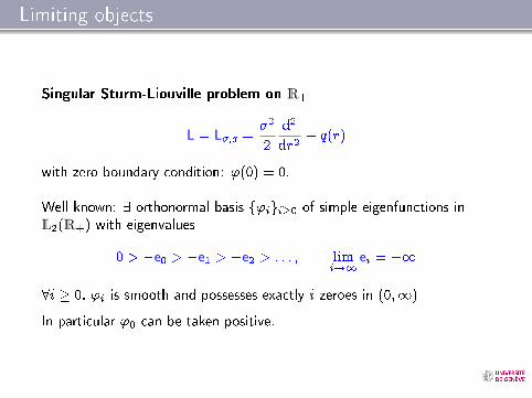
Singular Sturm-Liouville problem on R+

L = L�;q =�2

2

d2

dr2� q(r)

with zero boundary condition: '(0) = 0.

Well-known: 9 orthonormal basis f'igi�0 of simple eigenfunctions inL2(R+) with eigenvalues

0 > �e0 > �e1 > �e2 > : : : ; limi!1

ei = +1

8i � 0, 'i is smooth and possesses exactly i zeroes in (0;1)

In particular '0 can be taken positive.

Limiting objects

Singular Sturm-Liouville problem on R+

L = L�;q =�2

2

d2

dr2� q(r)

with zero boundary condition: '(0) = 0.

Well-known: 9 orthonormal basis f'igi�0 of simple eigenfunctions inL2(R+) with eigenvalues

0 > �e0 > �e1 > �e2 > : : : ; limi!1

ei = +1

8i � 0, 'i is smooth and possesses exactly i zeroes in (0;1)

In particular '0 can be taken positive.

Limiting objects

Ferrari-Spohn di�usions on (0;1)

Generators:

G�;q =1

'0(L+ e0I)( '0) =

�2

2

d2

dr2+ �2

'00'0

d

dr

The corresponding di�usions are ergodic and reversible w.r.t.

�0(dr) = '20(r)dr

Stationary path measure: P�;q

Limiting objects


Generators:

G�;q =1

'0(L+ e0I)( '0) =

�2

2

d2

dr2+ �2

'00'0

d

dr


�0(dr) = '20(r)dr


Limiting objects


Generators:

G�;q =1

'0(L+ e0I)( '0) =

�2

2

d2

dr2+ �2

'00'0

d

dr


�0(dr) = '20(r)dr


Main result

I Scaled process: x�(t) =1H�X[H2

�t] (with linear interpolation)

Theorem (Io�e, Shlosman, V., 2014)

Let (�N )N�1 be such that �N # 0 and H2�N=N ! 0. Then,

Law of x�N under Pu;vN;+;�N

N!1=) P�;q;

uniformly in 0 � u; v � CH�.

Main result

Example: V�(x) = �xIn this case:

H� = ��1=3; '0(r) = Ai(�r � !1); e0 =!1�;

where �!1 is the �rst zero of the Airy function Ai and � = 3p2=�2.

Scaling limit: di�usion in log-Airy potential

The corresponding di�usion was already derived in[Ferrari&Spohn, AoP 2005] in the context of aBrownian bridge conditioned to stay above a circularbarrier.

Main result

Example: V�(x) = �xIn this case:

H� = ��1=3; '0(r) = Ai(�r � !1); e0 =!1�;

where �!1 is the �rst zero of the Airy function Ai and � = 3p2=�2.

Scaling limit: di�usion in log-Airy potential

The corresponding di�usion was already derived in[Ferrari&Spohn, AoP 2005] in the context of aBrownian bridge conditioned to stay above a circularbarrier.

Transfer operator

(To simplify, I assume here that px = p�x)

8x; y 2 N; eT�(x; y) = py�x e�12 (V�(x)+V�(y))

Note that e12 (V�(u)+V�(v)) Z

u;vN;+;� = eT2N

� (u; v)

Krein-Rutman =) eT� possesses a leading e.f. �� > 0 of e.v. E�

Normalized version: T� = 1E�

eT�Ground-state chain:

��(x; y) =1

��(x)T�(x; y)��(y)

Pos. recurrent Markov chain, with inv. meas. ��(x) = c��(x)2

Stationary path-measure: P�

Transfer operator




u;vN;+;� = eT2N

� (u; v)




��(x; y) =1

��(x)T�(x; y)��(y)



Transfer operator




u;vN;+;� = eT2N

� (u; v)



eT�

Ground-state chain:

��(x; y) =1

��(x)T�(x; y)��(y)



Transfer operator




u;vN;+;� = eT2N

� (u; v)




��(x; y) =1

��(x)T�(x; y)��(y)



Convergence of fdds

Let N� = H�1� N.

E�fu0(x�(0))u1(x�(t))g =Xr;s2N�

��(H�r)�[H2

�t]

� (H�r; H�s)u0(r)u1(s)

Assume one can show that, as � # 0,

H�c� ! 1; ��(H�r) ! '0(r); T[H2

�t]

� [f�](H�r) ! Tt[f ](r)

where Tt = e(L+e0I)t and f�(H��) ! f(�).Xr2N�

��(H�r) � � � = c�

Xr2N�

��(H�r)2 � � � !

Zdr'0(r)

2 � � � =

Z�0(dr) � � �

andXs2N�

�[H2

�t]

� [u1(H�1� �)](H�r) =

1

��(H�r)T[H2

�t]

� [��u1(H�1� �)](H�r)

!1

'0(r)Tt['0u1](r) = e

G�;qt[u1](r)

Thus,E�fu0(x�(0))u1(x�(t))g ! E�;qfu0(x(0))u1(x(t))g

Convergence of fdds

Let N� = H�1� N.

E�fu0(x�(0))u1(x�(t))g =Xr;s2N�

��(H�r)�[H2

�t]

� (H�r; H�s)u0(r)u1(s)


H�c� ! 1; ��(H�r) ! '0(r); T[H2

�t]

� [f�](H�r) ! Tt[f ](r)

where Tt = e(L+e0I)t and f�(H��) ! f(�).

Xr2N�

��(H�r) � � � = c�

Xr2N�

��(H�r)2 � � � !

Zdr'0(r)

2 � � � =

Z�0(dr) � � �

andXs2N�

�[H2

�t]

� [u1(H�1� �)](H�r) =

1

��(H�r)T[H2

�t]

� [��u1(H�1� �)](H�r)

!1

'0(r)Tt['0u1](r) = e

G�;qt[u1](r)


Convergence of fdds

Let N� = H�1� N.

E�fu0(x�(0))u1(x�(t))g =Xr;s2N�

��(H�r)�[H2

�t]

� (H�r; H�s)u0(r)u1(s)


H�c� ! 1; ��(H�r) ! '0(r); T[H2

�t]

� [f�](H�r) ! Tt[f ](r)


��(H�r) � � � = c�

Xr2N�

��(H�r)2 � � � !

Zdr'0(r)

2 � � � =

Z�0(dr) � � �

andXs2N�

�[H2

�t]

� [u1(H�1� �)](H�r) =

1

��(H�r)T[H2

�t]

� [��u1(H�1� �)](H�r)

!1

'0(r)Tt['0u1](r) = e

G�;qt[u1](r)


Convergence of fdds

Let N� = H�1� N.

E�fu0(x�(0))u1(x�(t))g =Xr;s2N�

��(H�r)�[H2

�t]

� (H�r; H�s)u0(r)u1(s)


H�c� ! 1; ��(H�r) ! '0(r); T[H2

�t]

� [f�](H�r) ! Tt[f ](r)


��(H�r) � � � = c�

Xr2N�

��(H�r)2 � � � !

Zdr'0(r)

2 � � � =

Z�0(dr) � � �

andXs2N�

�[H2

�t]

� [u1(H�1� �)](H�r) =

1

��(H�r)T[H2

�t]

� [��u1(H�1� �)](H�r)

!1

'0(r)Tt['0u1](r) = e

G�;qt[u1](r)


Three main probabilistic inputs

1. The free energy is of order H�2�

Setting e� = �H2� logE�, this implies that

0 < lim inf�#0

e� � lim sup�#0

e� <1:

compactness of (e�)�>0

2. Tail estimate:

Pu;vN;+;�N

(X0 > KH�) � exp��K

�pq(K) ^H�

�uniformly in K > 0 and � � �0.

tightness of (x�;P�) and compactness of (��(H��))�>0

3. Approximation by stationary distributionSuppose N � H2

�Nand uN ; vN � cH�N . Then, for any local event A,

limN!1

jPu;vN;+;�N

(A)� P�N (A)j = 0:

su�cient to prove convergence of fdd under P�N




0 < lim inf�#0


e� <1:


2. Tail estimate:

Pu;vN;+;�N

(X0 > KH�) � exp��K

�pq(K) ^H�





limN!1

jPu;vN;+;�N

(A)� P�N (A)j = 0:





0 < lim inf�#0


e� <1:


2. Tail estimate:

Pu;vN;+;�N

(X0 > KH�) � exp��K

�pq(K) ^H�





limN!1

jPu;vN;+;�N

(A)� P�N (A)j = 0:


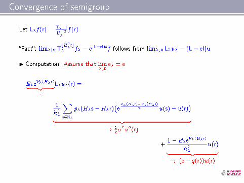
Convergence of semigroup

Let L�f(r) =T��I

H�2�

f(r)

�Fact�: lim�#0 TbH2

�tc

� f� = e(L+eI)tf follows from lim�#0 L�u� = (L+ eI)u

I Computation: Assume that lim�#0

e� = e

E�eV�(H�r)| {z }!1

L�u�(r) =

1

h2�

Xs2N�

p�(H�s�H�r)�eV�(H�r)�V�(H�s)

2 u(s)� u(r)�

| {z }! 1

2�2u00(r)

+1� E�e

V�(H�r)

h2�

u(r)| {z }! (e� q(r))u(r)



H�2�

f(r)


�tc



e� = e

E�eV�(H�r)| {z }!1

L�u�(r) =

1

h2�

Xs2N�


2 u(s)� u(r)�

| {z }! 1

2�2u00(r)

+1� E�e

V�(H�r)

h2�

u(r)| {z }! (e� q(r))u(r)



H�2�

f(r)


�tc



e� = e

E�eV�(H�r)| {z }!1

L�u�(r) =

1

h2�

Xs2N�


2 u(s)� u(r)�

| {z }! 1

2�2u00(r)

+1� E�e

V�(H�r)

h2�

u(r)| {z }! (e� q(r))u(r)

Identi�cation of the limit

One then easily deduce:

Proposition

e0 = lim�#0

e�; '0(r) = lim�#0

��(H�r)

Indeed, w.l.o.g., consider a subsequence (�k)k>0 such that e�k ! e and��k(H�k �)! '(�)

T�� = �� =) e(L+eI)t' = '

=) ' is a non-negative (normalized) eigenfunction of L witheigenvalue �e.

=) ' = '0 and e = e0



Proposition

e0 = lim�#0

e�; '0(r) = lim�#0

��(H�r)


T�� = �� =) e(L+eI)t' = '


=) ' = '0 and e = e0



Proposition

e0 = lim�#0

e�; '0(r) = lim�#0

��(H�r)


T�� = �� =) e(L+eI)t' = '


=) ' = '0 and e = e0



Proposition

e0 = lim�#0

e�; '0(r) = lim�#0

��(H�r)


T�� = �� =) e(L+eI)t' = '


=) ' = '0 and e = e0



Proposition

e0 = lim�#0

e�; '0(r) = lim�#0

��(H�r)


T�� = �� =) e(L+eI)t' = '


=) ' = '0 and e = e0

Thanks

for your attention!

Date post:	01-Sep-2019
Category:	Documents
Upload:	others
View:	1 times
Download:	0 times

Scaling limit of a layer of unstable...

Documents