648
LEARNING AND APPROXIMATE DYNAMIC PROGRAMMING Scaling Up to the Real World

LEARNINGANDAPPROXIMATE DYNAMICPROGRAMMING
Scaling Up to the Real World


LEARNINGANDAPPROXIMATE DYNAMICPROGRAMMING
Scaling Up to the Real World
Edited by
Jennie Si, Andy Barto, Warren Powell,and Donald Wunsch
A Wiley-Interscience Publication
JOHN WILEY & SONS
New York • Chichester • Weinheim • Brisbane • Singapore • Toronto

Preface
Complex artificial systems have become integral and critical components of modernsociety. The unprecedented rate at which computers, networks, and other advancedtechnologies are being developed ensures that our dependence on such systems willcontinue to increase. Examples of such systems include computer and communicationnetworks, transportation networks, banking and finance systems, electric power grid,oil and gas pipelines, manufacturing systems, and systems for national defense.These are usually multi-scale, multi-component, distributed, dynamic systems. Whileadvances in science and engineering have enabled us to design and build complexsystems, comprehensive understanding of how to control and optimize them is clearlylacking.There is an enormous body of literature describing specific methods for controllingspecific complex systems based on various simplifying assumptions and requiringa range of performance compromises. While much has been said about complexsystems, these systems are usually too complicated for the conventional mathematicalmethodologies that have proven to be successful in designing instruments. The mereexistence of complex systems does not necessarily mean that they are operatingunder the most desirable conditions with enough robustness to withstand the kindsof disturbances that inevitably arise. This was made clear, for example, by the majorpower outage across dozens of cities in the Eastern United States and Canada inAugust of 2003.Dynamic programming is a well-known, general-purpose method to deal with com-plex systems, to find optimal control strategies for nonlinear and stochastic dynamicsystems. It is based on the Bellman equation which suffers from a severe “curse ofdimensionality” (for some problems, there can even bethreecurses of dimensional-ity). This has limited its applications to very small problems. The same may be saidof the classical “min-max” algorithms for zero-sum games, which are closely related.Over the past two decades, substantial progress has been made through efforts inmultiple disciplines such as adaptive/optimal/robust control, machine learning, neuralnetworks, economics, and operations research. For the most part, these efforts havenot been cohesively linked, with multiple parallel efforts sometimes being pursuedwithout knowledge of what others have done. A major goal of the 2002 NSF workshopwas to bring these parallel communities together to discuss progress and to share ideas.Through this process, we are hoping to better define a community with commoninterests and to help develop a common vocabulary to facilitate communication.
Despite the diversity in the tools and languages used, a common focus of theseresearchers has been to develop methods capable of finding high-quality approximatesolutions to problems whose exact solutions via classical dynamic programming arenot attainable in practice due to high computational complexity and lack of accurateknowledge of system dynamics. At the workshop, the phraseapproximate dynamicprogramming(ADP) was identified to represent this stream of activities.A number of important results were reported at the workshop, suggesting that thesenew approaches based on approximating dynamic programming can indeed scale upto the needs of large-scale problems that are important for our society. However,to translate these results into systems for the management and control of real-worldcomplex systems will require substantial multi-disciplinary research directed towardintegrating higher-level modules, extending multi-agent, hierarchical, and hybridsystems concepts. There is a lot left to be done!This book is a summary of the results presented at the workshop, and is organizedwith several objectives in mind. First, it introduces the common theme of ADP toa large, interdisciplinary research community to raise awareness and to inspire moreresearch results. Second, it provides readers with detailed coverage of some existingADP approaches, both analytically and empirically, which may serve as a baseline todevelop further results. Third, it demonstrates the successes that ADP methods havealready achieved in furthering our ability to manage and optimize complex systems.The organization of the book is as follows. It starts with a strategic overview and futuredirections of the important field of ADP. The remainder contains three parts. PartOne aims at providing readers a clear introduction of some existing ADP frameworksand details on how to implement such systems. Part Two presents important andadvanced research results that are currently under development and that may lead toimportant discoveries in the future. Part Three is dedicated to applications of variousADP techniques. These applications demonstrate how ADP can be applied to largeand realistic problems arising from many different fields, and they provide insightsfor guiding future applications.Additional information about the 2002 NSF workshop can be found athttp://www.eas.asu.edu/˜nsfadp
Jennie SiTempe, AZ
Andrew G. BartoAmherst, MA
Warren B. PowellPrinceton, NJ
Donald C. WunschRolla, MO
April 14, 2004
i

Acknowledgments
The contents of this book are based on the workshop: “Learning and ApproximateDynamic Programming,” which was sponsored by the National Science Founda-tion (NSF grant number ECS-0223696), and held in Playacar, Mexico in April of2002. This book is a result of active participation and contribution from the workshopparticipants and the chapter contributors. Their names and addresses are listed below.
Charles W. AndersonDepartment of Computer ScienceColorado State UniversityFort Collins, CO 80523 USA
S. N. BalakrishnanDepartment of Mechanical and Aerospace Engineering and Engineering MechanicsUniversity of Missouri-RollaRolla, MO 65409 USA
Andrew G. BartoDepartment of Computer ScienceUniversity Of MassachusettsAmherst, MA 01003 USA
Dimitri P. BertsekasLaboratory for Information and Decision SystemsMassachusetts Institute of TechnologyCambridge, MA 02139 USA
Zeungnam BienDepartment of Electrical Engineering and Computer ScienceKorea Advanced Institute of Science and TechnologyYuseong-gu, Daejeon 305-701 Republic of Korea
Vivek S. BorkarSchool of Technology and Computer ScienceTata Institute of Fundamental Research
ii

ACKNOWLEDGMENTS iii
Mumbai, 400005 India
Xi-Ren CaoDepartment of Electrical and Electronic EngineeringHong Kong University of Science and TechnologyClear Water Bay, Kowloon , Hong Kong
Daniel Pucci de FariasDepartment of Mechanical EngineeringMassachusetts Institute of TechnologyCambridge, MA 02139 USA
Thomas G. DietterichSchool of Electrical Engineering and Computer ScienceOregon State UniversityCorvallis, OR 97331 USA
Russell EnnsBoeing Company the Helicopter Systems5000 East McDowell RoadMesa, AZ 85215
Department of Electrical EngineeringArizona State UniversityTempe, AZ 85287 USA
Augustine O. EsogbueIntelligent Systems and Controls LaboratoryGeorgia Institute of TechnologyAtlanta, GA 30332 USA
Silvia FerrariDepartment of Mechanical Engineering and Materials ScienceDuke UniversityDurham, NC 27708 USA
Laurent El GhaouiDepartment of Electrical Engineering and Computer ScienceUniversity of California at BerkeleyBerkeley, CA 94720 USA
Mohammad GhavamzadehDepartment of Computer ScienceUniversity of Massachusetts
iv ACKNOWLEDGMENTS
Amherst, MA 01003 USA
Greg GrudicDepartment of Computer ScienceUniversity of Colorado at BoulderBoulder, CO 80309 USA
Dongchen HanDepartment of Mechanical and Aerospace Engineering and Engineering MechanicsUniversity of Missouri-RollaRolla, MO 65409 USA
Ronald G. HarleySchool of Electrical and Computer EngineeringGeorgia Institute of TechnologyAtlanta, GA 30332 USA
Warren E. Hearnes IIIntelligent Systems and Controls LaboratoryGeorgia Institute of TechnologyAtlanta, GA 30332 USA
Douglas C. HittleDepartment of Mechanical EngineeringColorado State UniversityFort Collins, CO 80523 USA
Dong-Oh KangDepartment of Electrical Engineering and Computer ScienceKorea Advanced Institute of Science and TechnologyYuseong-gu, Daejeon 305-701 Republic of Korea
Matthew KretchmarDepartment of Computer ScienceColorado State UniversityFort Collins, CO 80523 USA
George G. LendarisSystems Science and Electrical EngineeringPortland State UniversityPortland, OR 97207 USA
Derong LiuDepartment of Electrical and Computer EngineeringUniversity of Illinois at Chicago
ACKNOWLEDGMENTS v
Chicago, IL 60612 USA
Sridhar MahadevanDepartment of Computer ScienceUniversity of MassachusettsAmherst, MA 01003 USA
James A. MomohCenter for Energy Systems and ControlDepartment of Electrical EngineeringHoward UniversityWashington, DC 20059 USA
Angelia NedichAlphatech, Inc.Burlington, MA 01803 USA
James C. NeidhoeferAccurate Automation CorporationChattanooga, TN 37421 USA
Arnab NilimDepartment of Electrical Engineering and Computer SciencesUniversity of California at BerkeleyBerkeley, CA 94720 USA
Warren B. PowellDepartment of Operations Research and Financial EngineeringPrinceton UniversityPrinceton, NJ 08544 USA
Danil V. ProkhorovResearch and Advanced EngineeringFord Motor CompanyDearborn, MI 48124 USA
Khashayar RohanimaneshDepartment of Computer ScienceUniversity of MassachusettsAmherst, MA 01003 USA
Michael T. RosensteinDepartment of Computer ScienceUniversity of Massachusetts
vi ACKNOWLEDGMENTS
Amherst, MA 01003 USA
Malcolm RyanSchool of Computer Science & EngineeringUniversity of New South WalesSydney 2052 Australia
Shankar SastryDepartment of Electrical Engineering and Computer SciencesUniversity of California at BerkeleyBerkeley, CA 94720 USA
Jennie SiDepartment of Electrical EngineeringArizona State UniversityTempe, AZ 85287 USA
Ronnie SircarDepartment of Operations Research and Financial EngineeringPrinceton UniversityPrinceton, NJ 08544 USA
Robert F. StengelDepartment of Mechanical and Aerospace EngineeringPrinceton UniversityPrinceton, NJ 08544 USA
Georgios TheocharousArtificial Intelligence LaboratoryMassachusetts Institute of TechnologyCambridge, MA 02139 USA
Lyle UngarSchool of Engineering and Applied ScienceUniversity of PennsylvaniaPhiladelphia, PA 19104 USA
Benjamin Van RoyDepartment of Management Science and EngineeringStanford UniversityStanford, CA 94305 USA
Ganesh K. VenayagamoorthyDepartment of Electrical and Computer EngineeringUniversity of Missouri-Rolla
ACKNOWLEDGMENTS vii
Rolla, MO 65409 USA
Paul WerbosNational Science FoundationArlington, VA 22230 USA
David WhitePraesagus Corp.San Jose, CA 95128 USA
Bernard WidrowDepartment of Electrical EngineeringStanford UniversityStanford, CA 94305 USA
Donald C. WunschDepartment of Electrical and Computer EngineeringUniversity of Missouri-RollaRolla, MO 65409 USA
Lei YangDepartment of Electrical EngineeringArizona State UniversityTempe, AZ 85287 USA
Peter YoungDepartment of Electrical and Computer EngineeringColorado State UniversityFort Collins, CO 80523 USA
Edwin ZiviWeapons & Systems Engineering DepartmentU.S. Naval AcademyAnnapolis, MD 21402 USA
The editors would like to acknowledge the efforts of Mr. Lei Yang and Mr. JamesDankert of the Department of Electrical Engineering at Arizona State University, whoassisted in many aspects during the preparation of this book and performed muchof the electronic formatting of the book manuscript. The editors would also like toacknowledge the support from Ms. Catherine Faduska and Ms. Christina Kuhnenat IEEE Press. Finally, the editors would like to thank the reviewers and Dr. DavidFogel for their encouragement and helpful inputs that have helped enhance the book.

Dedication
To those with an open mind and the courage to go beyond the ordinary.
viii

Contents
Foreword 1Shankar Sastry
1 ADP: Goals, Opportunities and Principles 2Paul Werbos
1.1 Goals of This Book 2
1.2 Funding Issues, Opportunities and the Larger Context 4
1.3 Unifying Mathematical Principles and Roadmap of the Field 16
Part I Overview 45
2 Reinforcement Learning and its Relationship to Supervised Learning 47Andrew G. Barto and Thomas G. Dietterich
2.1 Introduction 47
2.2 Supervised Learning 48
2.3 Reinforcement Learning 50
2.4 Sequential Decision Tasks 54
2.5 Supervised Learning for Sequential Decision Tasks 58
2.6 Concluding Remarks 60
3 Model-based Adaptive Critic Designs 64Silvia Ferrari and Robert F. Stengel
3.1 Introduction 64
3.2 Mathematical Background and Foundations 66
3.3 Adaptive Critic Design and Implementation 73
3.4 Discussion 88
3.5 Summary 88
4 Guidance in the Use of Adaptive Critics for Control 95
ix

x CONTENTS
George G. Lendaris and James C. Neidhoefer
4.1 Introduction 95
4.2 Reinforcement Learning 96
4.3 Dynamic Programming 97
4.4 Adaptive Critics: “Approximate Dynamic Programming” 97
4.5 Some Current Research on Adaptive Critic Technology 101
4.6 Application Issues 103
4.7 Items For Future ADP Research 116
5 Direct Neural Dynamic Programming 123Jennie Si, Lei Yang and Derong Liu
5.1 Introduction 123
5.2 Problem Formulation 124
5.3 Implementation of Direct NDP 125
5.4 Comparisons 131
5.5 A Continuous State Control Problem 136
5.6 Call Admission Control for CDMA Cellular Networks 138
5.7 Conclusions and Discussions 144
6 The Linear Programming Approach to Approximate Dynamic Program-ming 150
Daniela Pucci de Farias
6.1 Introduction 150
6.2 Markov Decision Processes 155
6.3 Approximate Linear Programming 156
6.4 State-Relevance Weights and the Performance of ALP Policies 157
6.5 Approximation Error Bounds 159
6.6 Application to Queueing Networks 162
6.7 An Efficient Constraint Sampling Scheme 164
6.8 Discussion 169
7 Reinforcement Learning in Large, High Dimensional State Spaces 175Greg Grudic and Lyle Ungar
7.1 Introduction 175
7.2 Theoretical Results and Algorithm Specifications 181
7.3 Experimental Results 188
7.4 Conclusion 194
CONTENTS xi
8 Hierarchical Decision Making 199Malcolm Ryan
8.1 Introduction 199
8.2 Reinforcement Learning and the Curse of Dimensionality 200
8.3 Hierarchical Reinforcement Learning in Theory 205
8.4 Hierarchical Reinforcement Learning in Practice 213
8.5 Termination Improvement 217
8.6 Intra-behaviour learning 219
8.7 Creating behaviours and building hierarchies 221
8.8 Model-based Reinforcement Learning 221
8.9 Topics for Future Research 222
8.10 Conclusion 223
Part II Technical Advances 229
9 Improved Temporal Difference Methods with Linear Function Approxi-mation 231
Dimitri P. Bertsekas, Vivek S. Borkar, and Angelia Nedich
9.1 Introduction 231
9.2 Preliminary Analysis 237
9.3 Convergence Analysis 239
9.4 Relations Betweenλ-LSPE and Value Iteration 241
9.5 Relation Betweenλ-LSPE and LSTD 248
9.6 Computational Comparison ofλ-LSPE and TD(λ) 249
10 Approximate Dynamic Programming for High Dimensional ResourceAllocation Problems 256
Warren B. Powell and Benjamin Van Roy
10.1 Introduction 256
10.2 Dynamic Resource Allocation 257
10.3 The Curses of Dimensionality 260
10.4 Algorithms for Dynamic Resource Allocation 261
10.5 Mathematical programming 266
10.6 Approximate Dynamic Programming 270
10.7 Experimental Comparisons 272
10.8 Conclusion 274
11 Concurrency, Multiagency, and Partial Observability 279
xii CONTENTS
Sridhar Mahadevan, Mohammad Ghavamzadeh, Khashayar Rohanimanesh, and Geor-gios Theocharous
11.1 Introduction 279
11.2 Background 281
11.3 Spatiotemporal Abstraction of Markov Processes 283
11.4 Concurrency, Multiagency, and Partial Observability 288
11.5 Summary and Conclusions 300
12 Learning and Optimization - From a System Theoretic Perspective 305Xi-Ren Cao
12.1 Introduction 305
12.2 A General View of Optimization 307
12.3 Estimation of Potentials and Performance Derivatives 310
12.4 Gradient-Based Optimization 317
12.5 Policy Iteration 318
12.6 Constructing Performance Gradients with Potentials as BuildingBlocks 322
12.7 Conclusion 324
13 Robust Reinforcement Learning Using Integral-Quadratic Constraints 330Charles W. Anderson, Matt Kretchmar, Peter Young, and Douglas Hittle
13.1 Introduction 330
13.2 Integral-Quadratic Constraints and Stability Analysis 331
13.3 Reinforcement Learning in the Robust Control Framework 333
13.4 Demonstrations of Robust Reinforcement Learning 339
13.5 Conclusions 347
14 Supervised Actor-Critic Reinforcement Learning 351Michael T. Rosenstein and Andrew G. Barto
14.1 Introduction 351
14.2 Supervised Actor-Critic Architecture 353
14.3 Examples 358
14.4 Conclusions 367
15 BPTT and DAC: A Common Framework for Comparison 373Danil V. Prokhorov
15.1 Introduction 373
15.2 Relationship between BPTT and DAC 375

CONTENTS xiii
15.3 Critic representation 378
15.4 Hybrid of BPTT and DAC 382
15.5 Computational complexity and other issues 387
15.6 Two classes of challenging problems 389
15.7 Conclusion 393
Part III Applications 397
16 Near-Optimal Control Via Reinforcement Learning 399Augustine O. Esogbue and Warren E. Hearnes II
16.1 Introduction 399
16.2 Terminal Control Processes 400
16.3 A Hybridization: The GCS-∆ Controller 402
16.4 Experimental Investigation of the GCS-∆ Algorithm 414
16.5 Dynamic Allocation of Controller Resources 416
16.6 Conclusions and Future Research 419
17 Multiobjective Control Problems by Reinforcement Learning 425Dong-Oh Kang and Zeungnam Bien
17.1 Introduction 425
17.2 Preliminary 427
17.3 Policy Improvement Algorithm for MDP with Vector-valued Reward 432
17.4 Model-Free Multiple Reward Reinforcement Learning for FuzzyControl 435
17.5 Summary 445
18 Adaptive Critic Based Neural Network for Control-Constrained AgileMissile 455
S. N. Balakrishnan and Dongchen Han
18.1 Introduction 455
18.2 Problem Formulation and Solution Development 457
18.3 Minimum Time Heading Reversal Problem in a Vertical Plane 461
18.4 Use of Networks in Real-Time as Feedback Control 465
18.5 Numerical Results 465
18.6 Conclusions 468
19 Applications of Approximate Dynamic Programming in Power SystemsControl 471
Ganesh K Venayagamoorthy, Ronald G Harley, and Donald C Wunsch

xiv CONTENTS
19.1 Introduction 471
19.2 Adaptive Critic Designs and Approximate Dynamic Programming 475
19.3 General Training Procedure for Critic and Action Networks 485
19.4 Power System 486
19.5 Simulation and Hardware Implementation Results 488
19.6 Summary 502
20 Robust Reinforcement Learning for Heating, Ventilation, and Air Con-ditioning Control of Buildings 508
Charles W. Anderson, Douglas Hittle, Matt Kretchmar, and Peter Young
20.1 Introduction 508
20.2 Heating Coil Model and PI Control 512
20.3 Combined PI and Reinforcement Learning Control 513
20.4 Robust Control Framework for Combined PI and RL Control 516
20.5 Conclusions 520
21 Helicopter Flight Control Using Direct Neural Dynamic Programming 526Russell Enns and Jennie Si
21.1 Introduction 526
21.2 The Helicopter Model 529
21.3 Direct NDP Mechanism Applied to Helicopter Stability Control 531
21.4 Direct NDP Mechanism Applied to Helicopter Tracking Control 539
21.5 Reconfigurable Flight Control 544
21.6 Conclusions 547
22 Towards Dynamic Stochastic Optimal Power Flow 551James A. Momoh
22.1 Grand Overview of the Plan for the Future Optimal Power Flow(OPF) 551
22.2 Generalized Formulation of the OPF Problem 557
22.3 General Optimization Techniques Used in Solving the OPF Problem 561
22.4 State-of-the-Art Technology in OPF Programs: The Quadratic Inte-rior Point (QUIP) Method 565
22.5 Strategy for Future OPF Development 566
22.6 Conclusion 587
23 Control, Optimization, Security, and Self-healing of Benchmark PowerSystems 589
James A. Momoh and Edwin Zivi

CONTENTS xv
23.1 Introduction 589
23.2 Description of the Benchmark Systems 591
23.3 Illustrative Terrestrial Power System Challenge Problems 594
23.4 Illustrative Navy Power System Challenge Problems 605
23.5 Summary of Power System Challenges and Topics 620
23.6 Summary 624

Foreword
SHANKAR SASTRY
University of California, Berkeley
This is the foreword.
1
1 ADP: Goals, Opportunities andPrinciples
PAUL WERBOS
National Science Foundation
1.1 GOALS OF THIS BOOK
Is it possible to build a general-purpose learning machine, which can learn to maxi-mizewhateverthe user wants it to maximize, over time, in a strategic way, even whenit starts out from zero knowledge of the external world? Can we develop general-purpose software or hardware to “solve” the Hamilton-Jacobi-Bellman equation fortruly large-scale systems? Is it possible to build such a machine which works effec-tively in practice, even when the number of inputs and outputs is as large as what themammal brain learns to cope with? Is it possible that the human brain itself is sucha machine, in part? More precisely - could it be that the same mathematical designprinciples which we use to build rational learning-based decision-making machinesare also the central organizing principle of the human mind itself? Is it possible toconvert all the great rhetoric about “complex adaptive systems” into something whichactually works, in maximizing performance?
Back in 1970, few informed scientists could imagine that the answers to these ques-tions might ultimately turn out to be yes, if the questions are formulated carefully.But as of today, there is far more basis for optimism than there was back in 1970.Many different researchers, mostly unknown to each other, working in differentfields, have independently found promising methods and strategies for overcomingobstacles which once seemed overwhelming.
This part will summarize the overall situation and the goals of this book briefly butprecisely, in words. Part 1.2 will discuss the needs and opportunities for ADP systemsacross some important application areas. Part 1.3 will discuss the core mathematicalprinciples which make all of this real.
2
GOALS OF THIS BOOK 3
Goal-oriented people may prefer to read part 1.2 first, but bottom-up researchers mayprefer to jump immediately to part 1.3. The discussion of goals here and in section1.2 is really just a brief summary of some very complex lessons learned over time,which merit much more detailed discussion in another context.
This book will focus on the first three questions above. It will try to bring togetherthe best of what is known across many disciplines relevant to the question: howcan we developbettergeneral-purpose tools for doing optimization over time, byusing learning and approximation to allow us to handlelarger-scale, more difficultproblems? Many people have also studied the elusive subtleties of the follow-onquestions about the human brain and the human mind [1]; however, we will neverbe able to construct a good straw-man model of how the mammalian brain achievesthese kinds of capabilities, until we understand what these capabilities require ofanyinformation processing system onanyhardware platform, wet, dry, hard or ethereal.The first three questions are a difficult enough challenge by themselves.
As we try to answer these three questions, we need to constantly re-examine whatthey actually mean. What are we trying to accomplish here? What is a “generalpurpose” machine? Certainly no one will ever be able to build a system which isguaranteed to survive when it is given just a microsecond to adapt to a totally crazyand unprecedented kind of lethal shock from out of the blue. Mammal brains workamazingly well, but even they get eaten up sometimes in nature. But certainly, weneed to look for some ability to learn or converge at reasonable speed (as fast aspossible!) across a wide variety of complex tasks or environments. We need tofocus on the long-term goal of building systems for the general case of nonlinearenvironments, subject to random disturbances, in which our intelligent system getsto observe only a narrow, partial window into the larger reality it is immersed in.
In practical engineering, we, like nature, will usually not want to start our systems outin a state of zero knowledge. But even so, we can benefit from using learning systemspowerful enough that theycould converge to an optimum, even when starting fromzero. Many of us consider it a gross abuse of the English language when peopleuse the word “intelligent” to describe high-performance systems which are unable tolearn anything fundamentally new, on-line or off-line.
In many practical applications today, we can use ADP as a kind of offline numericalmethod, which tries to “learn” or converge to an optimal adaptive control policy for aparticular type of plant (like a car engine). But even in offline learning, convergencespeed is a major issue, and similar mathematical challenges arise.
Is it possibleto achieve the kind of general-purpose optimization capability weare focusing on here, as the long-term objective? Even today, there is only oneexact method for solving problems of optimization over time, in the general caseof nonlinearity with random disturbance: dynamic programming (DP). But exactdynamic programming is used only in niche applications today, because the “curseof dimensionality” limits the size of problems which can be handled. Thus in manyengineering applications, basic stability is now assured via conservative design, butoverall performance is far from optimal. (It is common to optimize or tweak acontrol parameter here and there, but that is not at all the same as solving the

4 ADP: GOALS, OPPORTUNITIES AND PRINCIPLES
dynamic optimization problem.) Classical, deterministic design approaches cannoteven address questions like: How can we minimize theprobability of disaster, incases where we cannot totally guarantee that a disaster is impossible?
There has been enormous progress over the past ten years in increasing the scale ofwhat we can handle withapproximateDP and learning; thus the goals of this bookare two-fold: (1) to begin to unify and consolidate these recent gains, scattered acrossdisciplines; and (2) to point the way to how we can bridge the gap between wherewe are now andthe next major watershedin the basic science - the ability to handletasks as large as what the mammal brain can handle, and even to connect to what wesee in the brain.
The term “ADP” can be interpreted either as “Adaptive Dynamic Programming”(with apologies to Warren Powell) or as “Approximate Dynamic Programming” (asin much of my own earlier work). The long-term goal is to build systems whichinclude both capabilities; therefore, I will simply use the acronym “ADP” itself.Various strands of the field have sometimes been called “reinforcement learning”or “adaptive critics” or “neurodynamic programming,” but the term “reinforcementlearning” has had many different meanings to many different people.
In order to reach the next major watershed here, we will need to pay more attentionto two major areas: (1) advancing ADP as such, the main theme of this book; (2)advancing the critical subsystems we will need as components of ADP systems,such as systems which learn better and faster how to make predictions in complexenvironments.
1.2 FUNDING ISSUES, OPPORTUNITIES AND THE LARGERCONTEXT
This book is the primary product of an NSF-sponsored workshop held in Mexicoin April 2002, jointly chaired by Jennie Si and Andrew Barto. The goals of theworkshop were essentially the same as the goals of this book. The workshop coveredsome very important further information, beyond the scope of the book itself, postedat http://www.eas.asu.edu/˜nsfadp.
The potential of this newly emerging area looks far greater if we cancombinewhathas been achieved across all the relevant disciplines, and put the pieces all together.There are substantial unmet opportunities here, including some “low lying fruit.”One goal of this book is to help us see what these opportunities would look like, ifone were to bring these strands together in a larger, more integrated effort. But asa practical matter, large funding in this area would require three things: (1) moreproposal pressure in the area; (2) more unified and effective communication of thelarger vision to the government and to the rest of the community; (3) more follow-through on the visionwithin the ADP community - including more cross-disciplinaryresearch and more unified education.
Greater cross-disciplinary cooperation is needed for intellectual reasons, as you willsee from this book. It is also needed for practical reasons. The engineering and

FUNDING ISSUES, OPPORTUNITIES AND THE LARGER CONTEXT 5
operations research communities have done a good job on the applications side,on the whole, while the computer science communities have done a good job oneducational outreach and infrastructure. We will need to combine both of thesetogether, more effectively, to achieve the full potential in either area.
At a lower level, the Control, Networks and Computational Intelligence (CNCI)program in the Electrical and Communication Systems (ECS) Division of NSF hasfunded extensive work related to ADP, including earlier workshops which led tobooks of seminal importance [2, 3]. The center of gravity of CNCI has been theIEEE communities interested in these issues (especially in neural networks and incontrol theory), but ECS also provided some of the early critical funding for Barto,Bertsekas and other major players in this field. ADP remains a top priority in CNCIfunding. It will benefit the entire community if more proposals are received in theseareas. The Knowledge and Cognitive Systems program in Intelligent InformationSystems (IIS) Division of NSF has also funded a great deal of work in related areas,and has joined with ECS in joint-funding many projects.
In the panels which I lead for CNCI, I ask them to think of the funding decision itselfas a kind of long-term optimization problem under uncertainty. The utility functionto be maximized is a kind of 50-50 sum of two major terms - the potential benefitto basic scientific understanding, and the potential benefit to humanity in general.These are also the main considerations to keep in mind when considering possiblefunding initiatives.
Occasionally, some researchers feel that these grand-sounding goals are too large andtoo fuzzy. But consider this analogy. When one tries to sell a research project toprivate industry, onemustaddress the ultimate bottom line. Proposals which are notwell-thought-out and specifically tuned to maximize the bottom line usually do notget funded by industry. The bottom line is different at NSF, but the same principleapplies. Strategic thinking is essential in all of these sectors. All of us need to reassessour work, strategically, on a regular basis, to try to maximize our own impact on thelarger picture.
The biggest single benefit of ADP research, in my personal view, is based on the hopethat answers to the first three questions in section 1.1 will be relevant to the furtherquestions, involving the brain and the mind. This hope is a matter for debate in thelarger world, where it contradicts many strands of inherited conventional wisdomgoing back for centuries. This book cannot do justice to those complex and seriousdebates, but the connection between those debates and what we are learning fromADP has been summarized at length elsewhere (e.g. [9, 52], with reference to furtherdiscussions.
1.2.1 Benefits to Fundamental Scientific Understanding
In practice, the fundamental scientific benefit of most of the proposals which I seecomes down to the long-term watershed discussed above. There are few questionsas fundamental in science as “What is Mind or intelligence?” Thus I generally askpanelists to evaluate what the impact might be of a particular project in allowing us

6 ADP: GOALS, OPPORTUNITIES AND PRINCIPLES
to get to the watershed earlier than we would without the project. Since we willclearly need some kind of ADP to get there, ADP becomes the top scientific priority.But - as this book will bring out - powerful ADP systems will also require powerfulcomponentsor subsystems. This book will touch on some of the critical needs andopportunities for subsystems, such as subsystems which learn to predict or modelthe external world, subsystems for memory, subsystems for stochastic search andsubsystems for more powerful function approximation. This book may be uniquelyimportant in identifying what we need to get from such subsystems, but there areother books which discuss those areas in more detail. CNCI funds many projectsin those areas from people who may not know what ADP is, but are providingcapabilities important to the long-term goals. Likewise, there are many projects incontrol system design which can feed into the long-term goal here, with or withoutan explicit connection to ADP. In every one of these areas, greater unification ofknowledge is needed, for the sake of deeper understanding, more effective education,and reducing the common tendencies towards reinventing or spinning wheels.
1.2.2 Broader Benefits to Humanity
Optimal performance turns out to be critical to a wide variety of engineering andmanagement tasks important to the future of humanity - tasks which provide excellenttest-beds or drivers for new intelligent designs. The ECS Division has discussed thepractical needs of many major technology areas, directly relevant to the goals ofachieving sustainable growth here on earth, of cost-effective settlement of space, andof fostering human potential in the broadest sense. ADP has important potentialapplications in many areas, such as manufacturing [3], communications, aerospace,Internet software and defense, all of interest to NSF; however, test-beds related toenergy and the environment have the closest fit to current ECS activities.
This past year, ECS has played a major role in three cross-agency funding activi-ties involving energy and the environment, where ADP could play a critical role inenabling things which could not be done without it. It looks to me as if all threewill recur or grow, and all three are very open to funding partnerships between ADPresearchers and domain experts. The three activities focus on: (1) new crossdisci-plinary partnerships addressing electric power networks (EPNES); (2) space solarpower (JIETSSP); and (3) sustainable technology (TSE). To learn about these activi-ties in detail, search on these acronyms at http://www.nsf.gov. Here I will talk aboutthe potential role of ADP in these areas.
1.2.2.1 Potential Benefits In Electric Power Grids Computational intelligenceis only one of the core areas in the CNCI program. CNCI is also the main fundingprogram in the US government for support of electric utility grid research. CNCI haslong-standing ties with the IEEE Power Engineering Society (PES) and the ElectricPower Research Institute (EPRI). Transitions and flexibility in the electric powersector will be crucial to hopes of achieving a sustainable global energy system. Many
FUNDING ISSUES, OPPORTUNITIES AND THE LARGER CONTEXT 7
people describe the electric power system of the Eastern United States as “The largest,most complicated single machine ever built by man.”
The workshop led by Si and Barto was actually just one oftwo coordinated work-shops held back-to-back in the same hotel in Mexico. In effect, the first workshopasked: “How can we develop the algorithms needed in order to better approximateoptimal control over time of extremely large, noisy, nonlinear systems?” The secondworkshop, chaired by Ron Harley of the University of Natal (South Africa) and Geor-gia Tech, asked: “How can we develop the necessary tools in order to do integratedglobal optimization over time of the electric power grid as one single system?” Itis somewhat frightening that some engineers could not see how there could be anyconnection between these two questions, when we were in the planning stages.
The Harley workshop - sponsored by James Momoh of NSF and Howard Univer-sity, and by Massoud Amin of EPRI and the University of Minnesota - was actuallyconceived by Karl Stahlkopf, when he was a Vice-President of EPRI. Ironically,Stahlkopf urged NSF to co-sponsor a workshop on that topic as a kind of act of reci-procity for EPRI co-sponsoring a workshop I had proposed (when I was temporarilyrunning the electric power area) on hard-core transmission technology and urgentproblems in California. Stahlkopf was very concerned by the growing difficultyof getting better whole-system performance and flexibility in electric power grids,at a time when nonlinear systems-level challenges are becoming more difficult butcontrol systems and designs are still mainly based on piecemeal, local, linear or staticanalysis. “Is it possible,” he stressed, “to optimize thewhole thing in an integratedway, as a single dynamical system?”
It will require an entire new book to cover all the many technologies and needs foroptimization discussed at the second workshop. But there are five points of particularrelevance here.
First, James Momoh showed how his new Optimal Power Flow (OPF) system - beingwidely distributed by EPRI - is much closer to Stahlkopf’s grand vision than anythingelse now in existence.
Real-world suppliers to the electric utility industry have told me that OPF is farmore important to their clients than all the other new algorithms put together. OPFdoes provide a way of coordinating and integrating many different decisions acrossmany points of the larger electric power system. Momoh’s version of OPF - using acombination of nonlinear interior point optimization methods and genetic algorithms- has become powerful enough to cope with a growing variety of variables, all acrossthe system. But even so, the system is “static” (optimizes at a given time slice) anddeterministic. Stahlkopf’s vision could be interpretedeither as: (1) extending OPFto the dynamic stochastic case - thus creating dynamic stochastic OPF (DSOPF); (2)applying ADP to the electric power grid. The chances of success here may be best ifboth interpretations are pursued together in a group which understands how they areequivalent, both in theory and in mathematical details. Howard University may beparticularly well equipped to move towards DSOPF in this top-down, mathematically-based approach.

8 ADP: GOALS, OPPORTUNITIES AND PRINCIPLES
Some researchers in electric power are now working to extend OPF by adding the "S"but not the "D." They hope to learn from the emerging area of stochastic programmingin operations research. This can improve the treatment of certain aspects of powersystems, but it does provide a capability for anticipatory optimization. It does notprovide a mechanism for accounting for the impact of present decisions on futuresituations. For example, it would not give credit to actions that a utility system couldtake at present in order to prevent a possible "traffic jam" or breakdown in the nearfuture. Simplifications and other concepts from stochastic programming could bevery useful within the context of a larger, unifying ADP system, but only ADP isgeneral enough to allow a unified formulation of the entire decision problem.
Second, Venayagamoorthy of Missouri-Rolla presented important results which forma chapter of this book. He showed how DHP - a particular form of ADP design -results in an integrated control design for a system of turbogenerators which is ableto keep the generators up, even in the face of disturbances three times as large aswhat can be handled by the best existing alternative methods. This was shown onan actual experimental electric power grid in South Africa. The neural networkmodels of generator dynamics were trained in real time as part of this design. Theability to keep generators going is very useful in a world where containing andpreventing system-wide blackouts is a major concern. This work opens the door totwo possible extensions: (1) deployment on actual commercially running systems, inareas where blackouts are a concern or where people would like to run generators at ahigher load (i.e. with lower stability margins); (2) research into building up to largerand larger systems, perhaps by incorporating power-switching components into theexperimental networks and models. This may offer a “bottom-up” pathway towardsDSOPF. This work was an outcome of a CNCI grant to fund a partnership betweenRon Harley (a leading power engineer) and Don Wunsch (a leading researcher inADP from the neural network community).
Third, the DHP system used in this example outputs value signals which may beconsidered as “price signals” or “shadow prices.” They represent thegradientof themore conventional scalar value function used in the Bellman equation or in simplerADP designs. They are generalizations of the Lagrange Multipliers used in Momoh’sOPF system. They may also offer new opportunities for a better interface betweenthe computer-based grid control systems and the money-based economic controlsystems.
Fourth, there is every reason to worry that the technology used by Venayagamoorthy- which works fine for a dozen to a few dozen continuous state variables - will startto break down as we try to scale up to thousands of variables,unlessthe componentsof the design are upgraded, as I will discuss later in this chapter. The effort to scaleup is, once again, the core research challenge ahead of us here. One warning: somewriters claim to handle a dozen state variables when they actually mean that theyhandle a dozen possible states in a finite-state Markhov chain system; however, inthis case, I really am referring to a state space which is R12, a twelve-dimensionalspace defined by continuous variables, which is highly nonlinear, and not reducibleto clusters around a few points in that space.

FUNDING ISSUES, OPPORTUNITIES AND THE LARGER CONTEXT 9
Finally, ADP researchers who are interested in exploring this area are strongly urgedto look up “EPNES” at http://www.nsf.gov, and look in particular at the benchmarkproblems discussed there. The benchmark problems there, developed in collaborationbetween the two sponsors (NSF and the Navy), were designed to make it as easy aspossible for non-power-engineers to try out new control approaches. As a practicalmatter, however, EPNES is more likely to fund partnerships which do include acollaborator from hard-core power engineering.
1.2.2.2 Potential Benefits in Space Solar Power (SSP)The Millennium Project ofthe United Nations University (http://millennium-project.org) recently asked decisionmakers and science policy experts all over the world: “What challenges can sciencepursue whose resolution would significantly improve the human condition?” Theleading response was: “Commercial availability of a cheap, efficient, environmen-tally benign non-nuclear fission and non-fossil fuel means of generating base-loadelectricity, competitive in price with today’s fossil fuels.” Space solar power is a highrisk vision for future technology, but many serious experts believe that it is the mostpromising of the very few options for meeting this larger need. (Earth-based solaris another important option.) Thus in March 2002, NASA, NSF and EPRI issued asolicitation for proposals called the “Joint Investigation of Enabling Technologies forSpace Solar Power (JIETSSP).” John Mankins of NASA and I served as co-chairs ofthe Working Group which managed this activity.
Reducing costwas the number one goal of this effort. For each proposal, we askedthe reviewers to consider: What is the potential impact of funding this work onreducing the time we have to wait, before we know enough to build SSP systemswhich can safely beat the cost of nuclear power in developing regions like the MiddleEast? We also asked the usual questions NSF asks about the potential benefits tobasic science and other impacts.
Earlier proposals for SSP, dating back to the 1960’s and 1970’s, could not meet thiskind of cost target, for several reasons. One of the key problems was the enormouscost of sending up humans to do all of the assembly work in space. Consider thetotal costs of sending up six people to live in a space station, multiply by a thousand,and you begin to see how important it is to reduce this component of cost as much aspossible.
JIETSSP was partly the outcome of a workshop organized by George Bekey of USCin April 2000, jointly sponsored by NSF and NASA. The original goal was to explorehow radically new approaches to robotics, such as robots building robots or robotswith real intelligence, might be used to reduce costs either in space solar power or inbuilding earth-based solar power systems.
The most practical concept to emerge from that workshop was the concept of “teleau-tonomy” as described by Rhett Whittaker of Carnegie-Mellon. Truly autonomous,self-replicating robots may indeed become possible, using ADP and other new tech-nologies, but we do not really need them for SSP, and we need to make SSP affordableas soon as possible. But by the same token, we cannot afford to wait until domain
10 ADP: GOALS, OPPORTUNITIES AND PRINCIPLES
specialists in robotics develop complete three-dimensional physics models of everypossible task and every possible scenario that might occur in space.
Whittaker proposed that we plan for a system in which hundreds of human operators(mostly on earth) control hundreds or thousands of robots in space, to performassembly and maintenance. He proposed that we build up to this capability in anincremental way, by first demonstrating that we can handle the full range of requiredtasks in a more traditional telerobotics mode, and then focus on coordination and costreduction. Ivory tower robotics research can easily become a gigantic, unfocused,nonproductive swamp; Whittaker’s kind of strategy may be crucial to avoiding suchpitfalls. Greg Baiden, of Penguin ASI in Canada and Laurentian University, hasimplemented real-world teleautonomy systems used in the mining industry whichcan provide an excellent starting point. Lessons from assembling the InternationalSpace Station need to be accounted for as well.
In the short term, the most promising role for ADP in SSP robotics may be mid-levelwork, analogous to the work of Venayagamoorthy in electric power. Venayagamoor-thy has developed better sensor-based control policies, flexible enough to operateover a broader range of conditions, for acomponentof the larger power system. Inthe same way, ADP could be used to improve performance or robustness or autonomyfor componentsof a larger teleautonomy system. Half of the intellectual challengehere is to scope out the testbed challenges which are really important within realistic,larger systems designs in the spirit of Whittaker or Baiden.
What kinds of robotics tasks could ADP really help with, either in space or on earth?
Practical robotics in the US often takes a strictly domain-specific approach, in thespirit of expert systems. But the robotics field worldwide respects the achievementsof Hirzinger (in Germany) and Fukuda (in Japan), who have carefully developedways to use computational intelligence and learning to achieve better results in awide variety of practical tasks. Fukuda’s work on free-swinging, ballistic kinds ofrobots (motivated by the needs of the construction industry) mirrors the needs ofspace robotics far better than the domain-specific Japanese walking robots that havebecome so famous. Hirzinger has found ways to map major tasks in robotics into tasksfor general-purpose learning systems [4], where ADP(and related advanced designs)may be used to achieve capabilities even greater than what Hirzinger himself hasachieved so far.
It is also possible that new research, in the spirit of Warren Powell’s chapter in thisbook, could be critical to thelarger organizational problems in moving thousandsof robots and materials around a construction site in space. Powell’s methods forapproximating a value function have been crucial to his success so far in handlingdynamic optimization problems with thousands of variables - but even more powerfulfunction approximators might turn out to be important to SSP, if coupling effects andnonlinearities should make the SSP planning problems more difficult than the usuallogistics problems on earth. We do not yet know.
In 2002, JIETSSP funded twelve or thirteen research projects (depending on how onecounts). Five of these were on space robotics. These included an award to Singh,Whittaker and others at Carnegie-Mellon, and other projects of a more immediate
FUNDING ISSUES, OPPORTUNITIES AND THE LARGER CONTEXT 11
nature. They also included two more forwards-looking projects - one led by Shen atUSC and one by Jennie Si - aiming at longer-term, more fundamental improvementsin what can be done with robots. The Si project emphasizes ADP and what we canlearn from biology and animal behavior. The Shen project emphasizes robots whichcan adapt theirphysical form, in the spirit of Transformers, in order to handle a widerange of tasks.
A deep challenge to NASA and NSF here is the need to adapt to changes inhigh-leveldesign concepts for SSP. “What are we trying to build?” ask the roboticists. Butwe don’t yet know. Will it be something like the Sun Tower design which Mankins’groups developed a few years ago? Or will the core element be a gigantic light-to-light laser, made up of pieces “floating” in a vacuum, held together by some kind oftensegrity principle with a bit of active feedback control? Could there even be somekind of safe nuclear component, such as a laser fusion system in space, using thenew kinds of fuel pellets designed by Perkins of Lawrence Livermore which allowlight-weight MHD energy extraction from the protons emerging from D-D fusion? One should not even underestimate ideas like the Ignatiev/Criswell schemes forusing robotic systems to exploit materials on the moon. Given this huge spectrum ofpossibilities, we clearly need approaches to robotic assembly which are as flexibleand adaptive as possible.
1.2.2.3 Benefits to Technology for a Sustainable Environment (TSE)Com-plicated as they are, the electric power grid and the options for SSP are only twoexamples taken from a much larger set of energy/environment technologies of interestto the Engineering Directorate of NSF and to its partners. (For example, see [5].)
Many of the other key opportunities for ADP could now fit into the recently enlargedscope of Technology for a Sustainable Environment (TSE), a joint initiative of EPAand NSF. Recent progress has been especially encouraging for the use of intelligentcontrol in cars, buildings and boilers.
Building energy use is described at length in the chapter by Charles Anderson etal, based on a grant funded jointly by CNCI and by the CMS Division of NSF.Expert reviewers from that industry have verified that this new technology really doesprovide a unique opportunity to reduce energy use in buildings by a significant factor.Furthermore, use of ADP should make it possible to learn aprice-responsivecontrolpolicy, which would be very useful to the grid as a whole (and to saving money forthe customer). There are important possibilities for improved performance throughfurther research - but the biggest challenge for now is to transfer the success alreadyachieved in the laboratory to the global consumer market. There are no insuperablebarriers here, but it always takes a lot of time and energy to coordinate the manyaspects of this kind of fundamental transition in technology.
ADP for cars has larger potential, but the issues with cars are more complicated.There are urgent needs for reduced air pollution and improved fuel flexibility andefficiency in conventional cars and trucks. Many experts believe that the emissionof NOx compounds by cars and trucks is the main accessible cause of damage tohuman health and to nature today, from Los Angeles to the Black Forrest of Germany.

12 ADP: GOALS, OPPORTUNITIES AND PRINCIPLES
Improved fuel flexibility could be critical to the ability of advanced economies towithstand sharp reductions in oil supply from the Middle East ten years in the future- an issue of growing concern. In the longer term, cost and efficiency concerns willbe critical to the rate at which new kinds of cars – hybrid-electric, pure electric orfuel-cell cars - can actually penetrate the mass market.
Up to now, Feldkamp’s group at Ford Research has demonstrated the biggest provenopportunity for learning systems to yield important benefits here. By 1998, they haddemonstrated that a neural network learning system could meet three new stringentrequirements of the latest Clean Air Act in an affordable way, far better than any otherapproach ever proven out: (1) on-board diagnostics for misfires, using time-laggedrecurrent networks (TLRN); (2) idle speed control; (3) control of fuel/air ratios. InSeptember of 1998, the President of Ford committed himself (in a major interviewin Business Week) to deploying this system in every Ford car made in the world by2001. An important element of this plan was a new neural network chip design fromMosaix LLC of California (led by Raoul Tawel of the Jet Propulsion Laboratory),funded by an SBIR grant from NSF, which would cost on the order of $1-$10 perchip. Marko of Ford - who collaborates closely with Feldkamp’s group - was askedto organize a major conference on clean air technology for the entire industry, basedin part on this success.
But there are many caveats here.
First, there have been changes in the Clean Air Act in the past few years, and majorchanges in Ford management.
Second, management commitment by itself is not sufficient to change the basictechnology across a large world-wide enterprise, in the throes of other difficultchanges. The deployment of the lead element of the clean air system - the misfiredetector - has moved ahead very quickly, in actuality. Danil Prokhorov - who has animportant chapter in this book - has taken over a lead role in that activity, under LeeFeldkamp.
Third, the neural network control system was not based on ADP, and was not trainedto reduce NOx as such. Statistics on NOx reduction were not available, at lastcheck. The control system and the misfire detectors wereboth based on TLRNstrained by backpropagation through time (BTT [7]). In effect, they used the kind ofcontrol design discussed in section 2.10 of my 1974 PhD thesis on backpropagation[6], which was later implemented by four different groups by 1988 [2] includingWidrow’s famous truck-backer-upper, and was later re-interpreted as “neural modelpredictive control” ([3], ch. 10; [8]). Some re-inventions of the method havedescribed it as a kind of “direct policy reinforcement learning,” but it is not a formof ADP. It does not use the time-forwards kind of learning system required of aplausible model of brain-like intelligence. Some control engineers would call it akind of receding horizon method. Feldkamp’s group has published numerous paperson the key ideas which made their success possible, summarized in part in [4].
In his chapter, Prokhorov raises a number of questions about ADP versus BTT whichare very important in practical engineering. Properly implemented (as at Ford), BTTtends to be far superior in practice to other methods commonly used. Stability is

FUNDING ISSUES, OPPORTUNITIES AND THE LARGER CONTEXT 13
guaranteed under conditions much broader than what is required for stability withordinary adaptive control [8, 9]. Whenever BTT and ADP can both be applied to atask in control or optimization, a good evaluation study should use both on a regularbasis, to provide a kind of cross-check. Powell’s chapter gives one good example ofa situation where ADP works far better than a deterministic optimization. (Unlessone combines BTT with special tricks developed by Jacobsen and Mayne [10], BTTis a deterministic optimization method.) There are many connections between BTTand ADP which turn out to be important in advanced research, as Prokhorov andI have discussed. Many of the techniques used by Ford with BTT are essential tolarger-scale applications of ADP as well.
More recently, Jagannathan Sarangapani of the University of Missouri-Rolla hasdemonstrated a 50 percent reduction in NOx (with a clear possibility for getting itlower) in tests of a simple neural network controller on a Ricardo Hydra researchengine with cylinder geometry identical to that of the Ford Zetec engine [11], undera grant from CNCI. Sarangapani has drawn heavily on his domain knowledge fromyears of working at Caterpillar, before coming to the university. While BTT andADP both provide a way to maximize utility or minimize errorover the entire future,Sarangapani has used a simpler design which tries to minimize errorone time stepinto the future, using only one active “control knob” (fuel intake). But by using agood measure of error, and usingreal-time learning to update his neural networks,he was still able to achieve impressive initial results.
Saragapani explains the basic idea as follows. People have known for many yearsthat better fuel efficiency and lower NOx could be achieved, if engines could berun in a “lean regime” (fuel air ratios about 0.7) and if exhaust gasses could berecycled into the engine at a higher level. But in the past, when people did this,it resulted in a problem called “cyclic dispersion” - a kind of instability leading tomisfires and other problems. Physics-based approaches to modeling this problem andpreventing the instabilities have not been successful, because of real-world variationsand fluctuations in engine behavior. By using a simple neural network controller,inspired by ideas from his Ph.D. thesis adviser Frank Lewis [12], he was able toovercome this problem. This approach may lead to direct improvements in airquality from large vehicles which do not use catalytic converters (and are not likelyto soon, for many reasons).
As with the Anderson work, it will be important to take full advantage of the initialbreakthrough in performance here. But one can do better. One may expect betterperformance and extensions to the case of cars by incorporating greater foresight- by minimizing the same error or cost measure Sarangapani is already using, butminimizing it over the long-term, and multiplying it by a term to reflect the impactof fuel-oxygen ratios on the performance of the catalytic converter (or using a moredirect measure or predictor of emissions); ADP provides methods necessary to thatextension. ADP should also make it possible to account for additional “controlknobs” in the system, such as spark plug advance and such, which will be veryimportant to wringing out optimal performance from this system. It may also beimportant to use the approaches Ford has used to train TLRNs topredictthe system,
14 ADP: GOALS, OPPORTUNITIES AND PRINCIPLES
in order to obtain additionalinputsto the control systems, in order to really maximizeperformance and adaptability of the system. (See 3.2.2.) It may even be useful to usesomething like the Ford system topredict the likelihood of misfire, to construct anerror measure still better than what Saragapani is now using. In the end, theory tellsus to expect improved performance if we take such measures, but we will not knowhow large such improvements can actually be until we try our best to achieve them.
ADP may actually be more important tolonger-termneeds in the world of cars andtrucks.
For example, if mundane issues of mileage and pollution are enough to justify puttinglearning chips into all the cars and trucks in the world, then we can use those chipsfor additional purposes, without adding too much to the cost of a car. Years ago, thefirst Bush Administration made serious efforts to try to encouragedual-firedcars,able to flip between gasoline and methanol automatically. Roberta Nichols (nowwith UC Riverside) once represented Ford in championing this idea at a nationallevel. But at that time, it would have cost about $300 per car to add this flexibility,and oil prices seemed increasingly stable. In 2003 - it seems increasingly clearthat more “fuel insurance” would be a very good thing to have, andalso an easierthing to accomplish. Materials are available for multi-fuel gas tanks. It does nothave to be just gasolineor methanol; a wide spectrum can be accommodated. Butmore adaptive, efficient engine control becomes crucial. Learning-based controlmay provide a way to make that affordable. Fuel flexibility may also be importantin solving the “chicken and egg” problems on the way to a more sustainable mix ofenergy sources.
Cost and efficiency of control are central issues as well in hybrid, electric and fuelcell vehicles. As an example, chemical engineers involved in fuel cells have oftenargued that today’s fuel cell systems are far less efficient than they could be, if onlythey took better advantage of synergies like heat being generated in one place andneeded in another, with the right timing. Optimizationacross timeshould be able tocapture those kinds of synergies.
1.2.2.4 Benefits in Other Application Domains For reasons of space, I cannotdo real justice to the many other important applications of ADP in other areas. I willtry to say a little, but apologize to those who have done important work I will not getto.
Certainly the broader funding for ADP, beyond ECS, would benefit from greater useof ADP in other well-funded areas such as counterterrorism, infrastructure protectionabove and beyond electric power, health care, transportation, other branches ofengineering and software in general. Sometimes strategic partnerships with domainexperts and a focus on benchmark challenges in those other sectors are the best way toget started. When ECS funding appears critical to opening the door to large fundingfrom these other sources, many of us would bend over backwards to try to help,within the constraints of the funding process. In some areas - like homeland securityand healthcare, in particular - the challenges to humanity are so large and complexthat the funding opportunities available today may not always be a good predictor
FUNDING ISSUES, OPPORTUNITIES AND THE LARGER CONTEXT 15
of what may become available tomorrow, as new strategies evolve to address theunderlying problems more effectively.
Ferrari and Stengel in this book provide solid evidence for an astounding conclusion- namely, that significant improvements in fuel efficiency and maneuverability arepossible even for conventional aircraft and conventional maneuvers, using ADP. Sten-gel’s long track record in aerospace control and optimal control provides additionalevidence that we should take these results very seriously.
ADP clearly has large potential in “reconfigurable flight control (RFC),” the effort tocontrol aircraft so as to minimize the probability of losing the aircraft after damage sosevere that an absolute guarantee of survival is not possible. The large current effortsin RFC across many agencies (most notably NASA Ames) can be traced back tosuccessful simulation studies using ADP at McDonnell-Douglas, using McDonnell’sin-house model of its F-15 [3]. Mark Motter of NASA organized a special sessionat the American Control Conference (ACC01 Proceedings) giving current status andpossibilities. Lendaris’ work in this book was partly funded by NSF, and partlyfunded under Motter’s effort, in association with Accurate Automation Corporationof Tennessee. Jim Neidhoefer and Krishnakumar developed important ADP applica-tions in the past, and have joined the NASA Ames effort, where Charles Jorgensenand Arthur Soloway made important earlier contributions, particularly in developingverification and validation procedures.
It is straightforward to extend ADP for use in strategic games. Some of the hybridcontrol designs described by Shastry and others are general-purpose ADP designs,with clear applicability to strategic games, autonomous vehicles and the like. Balakr-ishnan has demonstrated success in hit-to-kill simulations (on benchmark challengesprovided by the Ballistic Missile Defense Organization) far beyond that of othercompetitors. As with electric power, however, upgradedcomponentsmay be crit-ical in making the transition from controlling one piece of the system, to optimalmanagement of the larger theater.
There is also a strong parallel between the goal of “value-based management” ofcommunication networks and the goal of DSOPF discussed in section 1.2.2.1. Inparticular, preventing “traffic jams” is essentially a dynamic problem, which staticoptimization and static pricing schemes cannot address as well.
Helicopter control and semiconductor manufacturing with ADP have been addressedby Jennie Si in this book, and by David White in [3] and in other places. Unmetopportunities probably exist to substantially upgrade the manufacturing of high-quality carbon-carbon composite parts, based on the methods proven out by Whiteand Sofge when they were at McDonnell-Douglas [3].
As this book was going to press, Nilesh Kulkarni of Princeton and Minh Phan ofDartmouth reported new simulations of the use of ADHDP in design of plasma hyper-sonic vehicles, a radically new approach to lower-cost reusable space transportation,where it is crucial to have a more adaptive nonlinear sort of control scheme like ADP.(This was jointly funded by CNCI and by the Air Force.) During the meeting atthe Wright-Patterson Air Force Base, the key aerospace designers and funders wereespecially enthusiastic about the possible application of ADP to “Design for Optimal
16 ADP: GOALS, OPPORTUNITIES AND PRINCIPLES
Dynamic Performance,” which we had asked Princeton to investigate. In DODP, thesimulator would contain truly vicious noise (reflecting parameter uncertainties), andADP would be used to tune both the weightsand the physical vehicle design pa-rameters so as to optimize performance over time. Researchers such as Frank Lewisand Balakrishnan have demonstrated promising systems and opportunities with Mi-croElectroMechanical Systems (MEMS), a key stream of nanotechnology. Manyforward-looking funding discussions stress how we are moving towards a new kindof global cyberinfrastructure, connecting in a more adaptive way from vast networksof sensors to vast networks of action and decision, with more and more fear that wecannot rely on Moore’s Law alone to keep improving computing throughput per dol-lar beyond 2015. ADP may provide a kind of unifying framework for upgrading thisnew cyberinfrastructure, especially if we develop ADP algorithms suitable for im-plementation on parallel distributed hardware (such as cellular neural networks)withanalog aspects (as in the work of Chris Diorio, funded by ECS).
Many researchers such as John Moody have begun to apply ADP or related methodsin financial decision-making. Older uses of neural networks in finance have taken a"behaviorist" or "technical" approach, in which the financial markets are predictedas if they were stochastic weather systems without any kind of internal intelligence.George Soros, among others, has argued very persuasively and very concretely howlimited and dangerous that approach can become (even though many players are saidto be making a lot of money in proprietary systems). The financial system itself maybe analyzed as a kind of value-calculation system or critic network. More concretely,the systems giving supply and demand (at a given price) may be compared to theAction networks or policy systems in an ADP design, and systems which adapt pricesto reflect supply and demand and other variables may be compared to certain types ofcritic systems (mainly DHP). The usual pricing systems assumed in microeconomicoptimality theorems tend to require perfect foresight, but ADP critics remain validin the stochastic case; thus they might have some value in areas like auction systemdevelopment, stability analysis, or other areas of economic analysis.
Again, of course, the work by Warren Powell on large-scale logistics problems is amajor watershed in showing how ADP can already outperform other methods, and isdoing so today on large important real-world management problems.
1.3 UNIFYING MATHEMATICAL PRINCIPLES AND ROADMAP OFTHE FIELD
1.3.1 Definition of ADP, Notation and Schools of Thought
The key premise of this book is that many different schools of thought, in differentdisciplines, using different notation have made great progress in addressing the sameunderlying mathematical design challenge. Each discipline tends to be fiercelyattached to its own notation, terminology and personalities - but here I will haveto choose a notation “in the middle” in order to discuss how the various strands of
UNIFYING MATHEMATICAL PRINCIPLES AND ROADMAP OF THE FIELD 17
research fit each other. I will try to give a relatively comprehensive review of themain ideas - but I hope that the important work which I do not know about will bediscussed in the more specialized reviews in other chapters of this book.
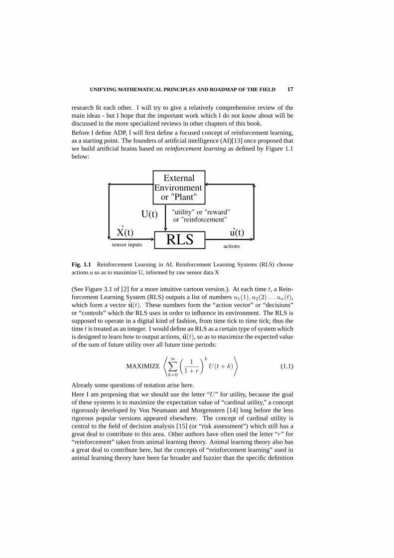
Before I define ADP, I will first define a focused concept of reinforcement learning,as a starting point. The founders of artificial intelligence (AI)[13] once proposed thatwe build artificial brains based onreinforcement learningas defined by Figure 1.1below:
RLS
ExternalEnvironment
or "Plant"
"utility" or "reward"or "reinforcement"
U(t)
u(t)
actionssensor inputs
X(t)
Fig. 1.1 Reinforcement Learning in AI. Reinforcement Learning Systems (RLS) chooseactions u so as to maximize U, informed by raw sensor data X
(See Figure 3.1 of [2] for a more intuitive cartoon version.). At each timet, a Rein-forcement Learning System (RLS) outputs a list of numbersu1(1), u2(2) . . . un(t),which form a vector~u(t). These numbers form the “action vector” or “decisions”or “controls” which the RLS uses in order to influence its environment. The RLS issupposed to operate in a digital kind of fashion, from time tick to time tick; thus thetimet is treated as an integer. I would define an RLS as a certain type of system whichis designed to learn how to output actions,~u(t), so as to maximize the expected valueof the sum of future utility over all future time periods:
MAXIMIZE
⟨ ∞∑
k=0
(1
1 + r
)k
U(t + k)
⟩(1.1)
Already some questions of notation arise here.
Here I am proposing that we should use the letter “U ” for utility, because the goalof these systems is to maximize the expectation value of “cardinal utility,” a conceptrigorously developed by Von Neumann and Morgenstern [14] long before the lessrigorous popular versions appeared elsewhere. The concept of cardinal utility iscentral to the field of decision analysis [15] (or “risk assessment”) which still has agreat deal to contribute to this area. Other authors have often used the letter “r” for“reinforcement” taken from animal learning theory. Animal learning theory also hasa great deal to contribute here, but the concepts of “reinforcement learning” used inanimal learning theory have been far broader and fuzzier than the specific definition

18 ADP: GOALS, OPPORTUNITIES AND PRINCIPLES
here. The goal here is to focus on a mathematical problem, and mathematicalspecificity is crucial to that focus.
Likewise, I am using the letter “r” for the usual discount rate or interest rate asdefined by economists for the past many centuries. It is often convenient, in puremathematical work, to define a discountfactorγ by:
γ =1
1 + r(1.2)
However, the literature of economics and operations research has a lot to say aboutthe meaning and use ofr which is directly relevant to the use of ADP in engineeringas well [16]. Some computer science papers discuss the choice ofγ as if it werepurely a matter of computational convenience - even in cases where the choice ofγmakes a huge difference to deciding what problem is actually being solved. Valuesof γ much less than one can be a disaster for systems intended to survive for morethan two or three time ticks.
From the viewpoint of economics, the control or optimization problems which we tryto solve in engineering are usually just subproblems of a larger optimization problem- the problem of maximizing profits or maximizing value-added for the companywhich pays for the work. To do justice to the customer, one should use an interestrater which is only a few percentper year. True, ethical foresight demands that wetry to setr = 0, in some sense, for the utility functionU which we use at the highestlevel of decision-making [16]. It is often more difficult to solve an optimizationproblem for the case wherer → 0; however, our ability to handle that case is just asimportant as our ability to scale up to larger plants and larger environments.
Finally, I am using angle brackets, taken from physics, to denote the expectationvalue.
There are many other notations for expectation value used in different disciplines;my choice here is just a matter of convenience and esthetics.
Over the years, the concept of an RLS in AI has become somewhat broader, fuzzierand not really agreed upon. I will define a more focused concept of RLS here, justfor convenience.
Much of the research on RLS in AI considers the case where the time horizon is notinfinite as in equation 1.1. That really is part of RLS research, and part of ADP aswell, so long as people are using the kinds of designs which can address the case ofan infinite time horizon. But when people address the classic problem of stochasticprogramming (i.e., when their future time horizon is just one period ahead), that is notADP. There are important connections between stochastic programming and ADP,just as there are connections between nonlinear programming and ADP, but they aredifferent mathematical tasks.
Likewise, in Figure 1.1, we are looking for an RLS design which marches forwardsin time, and can be scaled up “linearly” as the complexity of the task grows. It istricky to define what we mean by “linear scaling” in a precise way. (See [9] for aprecise statement for the particular case of Multiple-Input Multiple-Output (MIMO)
UNIFYING MATHEMATICAL PRINCIPLES AND ROADMAP OF THE FIELD 19
linear control.) But we certainly are not looking for designs whose foresight is totallybased on an explicit prediction of every time periodτ between the presentt and somefuture ultimate horizont+H. Designs of that sort are basically a competitor to ADP,as discussed in section 1.2.2.3. We are not looking for designs which include explicitsolution of theN2-by-N2 supraoperator [17] equations which allow explicit solutionof matrix Riccati equations. Nevertheless, ADP research does include researchwhich uses less scaleable components, if it uses themwithin scaleable designs and ifit teaches us something important to our long-term goals here.(e.g., [18, 19].)
ADP is almost the same as this narrow version of RLS,except thatwe assume thatutility is specified as a functionU(~X(t)) instead of just a “reinforcement signal”U(t).ADP is more general, because we could always append a “reinforcement signal” tothe vector~X(t) of current inputs, and defineU(~X) as the function which picks outthat component. ADP also includes the case where time t may be continuous.
In ADP, as in conventional control theory, we are interested in the general case ofpartially observedplants or environments. In my notation, I would say that the“environment” box in Figure 1.1 contains a “state vector,”~R(t), which is not thesame as~X(t). (In control theory [12, 20, 21], the state vector is usually denoted as~x, while the vector of observed or sensed data is called~y.) “R” stands for “reality.”Within an ADP system, we do not know the true value of~R(t), the true state ofobjective reality; however we may use Recurrent systems to Reconstruct or update aRepresentation of Reality. (See section 1.3.2.2.)
True ADP designs all include a component (or components) which estimates “value.”There are fundamental mathematical reasons why it is impossible to achieve the goalsdescribed here, without using “value functions” somehow. Some work in ADP, inareas like hybrid control theory, does not use the phrase “value function,” but thesekinds of functions are present under different names. Value functions are related toutility functions U, but are not exactly the same thing. In order to explain why valuefunctions are so important, we must move on to discuss the underlying mathematics.
1.3.2 The Bellman Equation, Dynamic Programming and Control Theory
Traditionally, there is only one exact and efficient way to solve problems in optimiza-tion over time, in the general case where noise and nonlinearity are present: dynamicprogramming. Dynamic programming was developed in the field of operations re-search, by Richard Bellman, who had close ties with John Von Neumann.
The basic idea of dynamic programming is illustrated in Figure 1.2:
In dynamic programming, the user supplies both a utility function - the function to bemaximized - and a stochastic model of the external plant or environment. One thensolves forthe unknown functionJ(~x(t)) which appears in the equation in Figure 1.2.This function may be viewed as a kind of secondary or strategic utility function. Thekey theorem in dynamic programming is roughly as follows: the strategy of action~u which maximizesJ in the immediate future (timet + 1) is the strategy of actionwhich maximizes the sum ofU over the long-term future (as in Eq. 1.2). Dynamic

20 ADP: GOALS, OPPORTUNITIES AND PRINCIPLES
Dynamic programming Dynamic programming
Model of reality Model of reality Utility function U Utility function U
Secondary, or strategic utility function J Secondary, or strategic utility function J
J( x (t)) = Max <U( x (t), u (t))+(J( x (t+1))/(1+r))> u (t)
Fig. 1.2 The basic idea of dynamic programming: given U, solve the Bellman equation toget J; use J to calculate optimal actions
programming converts a problem in optimization over time into a “simple” problemin maximizingJ just one step ahead in time.
1.3.2.1 Explanation of Basic Elements in Figure 1.2Before going further, weneed to explain Figure 1.2 very carefully. There are some hidden issues here whichare important even to advanced research in ADP.
The equation in Figure 1.2 is a variant of the original equation developed by Bellman.The task of optimization in the deterministic case, where there is no noise, was studiedcenturies before Bellman. Bellman’s equation was re-interpreted, years ago, as thestochastic generalization of the Hamilton-Jacobi equation of physics. Thus manycontrol theorists now refer to it as the “Hamilton-Jacobi-Bellman” (HJB) Equation.
Many people have found that DP or ADP can be useful even in the deterministiccase. The case of zero noise is just a special case of the general method. Many booksstart out by explaining DP in the case of zero noise, and then discussing the generalcase, which they call “stochastic dynamic programming.” But for researchers inthe field, “stochastic dynamic programming” is a redundant expression, like “mentaltelepathy.”
In Figure 1.2,J is the value function. Many researchers use “J” [15, 25], but manyothers - especially in AI - use “V ,” in part because of the seminal paper by Barto,Sutton and Anderson [26]. The idea is that “V ” stands for “value.” But there areother types of value function which occur in ADP research.
The equation in Figure 1.2 deviates a little from the original formulation of VonNeumann, insofar as the utility functionU is now shown as a function of the state~x(t) and of the actions~u(t). I did not include that extension, back in the firstcrude paper which proposed that we develop reinforcement learning systems byapproximating Howard’s version of dynamic programming [27, 22]. In that paper, Istressed the difference between primitive, unintelligent organisms - whose behavior is
UNIFYING MATHEMATICAL PRINCIPLES AND ROADMAP OF THE FIELD 21
governed by in-born automatic stimulus-response action responses - versus intelligentorganisms, which learn to choose actions based on theresultswhich the actions leadto. There is no real need for the extension toU(~x, ~u), since we can always accountfor variables like costs in the state vector. Nevertheless, the extension turns out tobe convenient for everyday operations research. When we make this extension, theoptimal~u(t) is no longer the~u(t) which maximizes <J(~x(t + 1))>; rather, it is the~u which maximizes <U(t) + J(t + 1)>, as shown in Figure 1.2.
The reader who is new to this area may ask where the stochastic model fits intothis equation. The stochastic model of reality is necessary in order to compute theexpectation values in the equation.
1.3.2.2 Partial Observability and Robust Control: Why “~x” in Figure 1.2 Is aCentral Problem Note that I used “~x” here to describe the state of the plant orenvironment. I deliberately did not write “~X” or “ ~R,” in Figure 1.2, because there isa very serious problem here, of central importance both in theory and in practice, inDP and in ADP. The problem is that classical DP assumes afully observed system.In other words, it assumes that the system which chooses~u(t) is able to make itsdecision based onfull knowledgeof ~x(t). More precisely, it assumes that we aretrying to solve for an optimal strategy or policy of action, which may be written as afunction~u(~x), and it assumes that the observed variables obey a Markhov process;in other words,~x(t + 1) is governed by a probability distribution which dependson~x(t) and~u(t), and is otherwise independent of anything which happened beforetime t. Failure to fully appreciate this problem and its implications has been a majorobstacle to progress in some parts of ADP research.
In control theory and in operations research, there has long been active researchinto Partially Observed Markhov Decision Problems (POMDP). ADP, as defined inthis book, is really an extension of the general case, POMDP, and not of DP in thenarrowest sense.
Control theory has developed many insights into partial observability. I cannotsummarize all of them here, but I can summarize a few highlights.
There are three very large branches of modern control theory - robust control, adaptivecontrol and optimal control. There are also some important emerging branches, likediscrete event dynamical systems (DEDS) and hybrid control, also represented inthis book. Even within control theory, there are big communication gaps betweendifferent schools of thought and different streams of practical applications.
Optimal control over time in thelinear case, for a known plant subject to Gaussiannoise, is a solved problem. There are several standard textbooks [20, 28]. Forthis kind of plant, an optimal controller can be designed by hooking together twocomponents: (1) a Kalman filter, which estimates the state vector~R(t), using a kindof recurrent update rule mainly based on the past~R(t− 1), the current observations~X(t) and the past actions~u(t − 1); (2) a “certainty equivalence” controller, whichis essentially the same as what DP would ask for,assuming thatthe estimated statevector is the true state vector. This kind of “certainty equivalence” approach is not
22 ADP: GOALS, OPPORTUNITIES AND PRINCIPLES
exactly correct in the nonlinear case, but it can be a useful approximation - far betterthan assuming that the state vector is just the same as the vector~X!
Robust and adaptive control are two different ways of responding to the question:“What can we do when the dynamics of the plant themselves are unknown?” Ro-bust control and adaptive control were both developed around the goal ofstability,first, rather than performance. In both cases, you usually assume that you have amathematical model of the plant to be controlled - but there are parameters in thatmodel whose values are unknown. In robust control, you try to find a control law orcontroller design~u(~X) which guarantees that the plant will not blow up, no matterwhat the unknown parameters are, over a very wide space of possibilities. There arecomputational tools now widely available for “mu synthesis” and such, which allowyou to maximize the margin of safety (the acceptable range of parameters) for theusual linear case. In adaptive control, you try toadaptyour control rule in real time,based on real-time observations of how the plant actually behaves. Note that adaptivedynamic programming (ADP) is not a special case of adaptive control in the usualsense!
Several advanced researchers in robust control, such as Athans and Barras, haveaddressed the task of robust controlin the general nonlinear case. It turns out thatthe solution to that task reduces to the task of trying to solve the HJB equation!Thus the most accurate possible approximation to true nonlinear robust control, inthe general case, can only be found by developing software which approximates thesolution to the HJB equation. From the viewpoint of nonlinear robust control, thisentire book can be seen as a book about the computational issues in implementingnonlinear robust control. But in actuality, when we use an HJB equation to derive arobust controller, we can add terms in the utility function to represent concepts likeenergy use and cost, to represent more accurately what we really want.
Barras [29] has done important fundamental work on partial observability in thiscase. Crudely, his work appears to say that we can solve for the true “optimal”nonlinear robust controller, if we take the certainty equivalence approach, but weuse a different kind of filter instead of the Kalman filter. We must use a nonlinearfunction approximator, and we must tune or train it so as to minimize a special lossfunction which properly penalizes different kinds of prediction errors. The reader isurged to study the original paper for a more precise statement of the findings. (See[9] and [20]and the chapter by Anderson et al in this book for some other connectionsbetween robust control, optimal control, adaptive control and ADP.)
Both in nonlinear robust controland in other ADP applications, there will always bea certain amount of approximation error in solving the HJB equations, no matter howhard we work to minimize that error. This does have some implications for stabilityanalysis, for real-world nonlinear robust control just as much as for other forms ofADP. As Balakrishnan has frequently argued, we know that the controller we getafter the factis stable, if we have found a way to converge to a reasonably accuratesolution of the HJB equation in off-line learning - even if we had to try out differentsets of initial weights to get there, and exploit tricks like “shaping” ([3], Foreword).

UNIFYING MATHEMATICAL PRINCIPLES AND ROADMAP OF THE FIELD 23
The problem of partial observability is crucial to practical applications, in many ways.For example, section 1.2.2.3 mentions the work by Ford Research in developing aclean car chip. Both Ford and Sarangapani have stressed how variations between onecar engine and another explain why classical types of control design (implemented atgreat detail and at great cost) failed to achieve the kind of success they were able toachieve.No fixed feedforward controller, conventional or neural, can be expected toperform well across such a wide range of plants. However, there are two approacheswhich have worked here: (1) as in Sarangapani, the approach of learning or adaptingin real time to the individual plant; (2) as at Ford, the use of a kind of certaintyequivalence approach.
In the simplest neural certainty equivalence approach (or “neural observer” approach,as described by Frank Lewis), we train a Time-Lagged Recurrent Network [3, 6] topredict the observed variables~X(t) as a function of~X(t−1), ~R(t−1) and~u(t−1),where R now represents a set of recurrent neurons. In fact, the combination of~X(t)and of this~R(t) is basically just an estimated state vector! When we make thisexpanded vector of inputs available to our policy,~u(~X, ~R), we arrive at a reasonableapproximation to the exact results of Stengel, Barras and others. The recurrenttunable prediction structure does not have to be a neural network - but for the generalnonlinear case, it should be some kind of universal nonlinear approximator.
Eventually, brain-like capability will require acombinationof real-time learning (tolearn the laws of nature, in effect) and time-lagged recurrence (to allow fast adaptationto changes in familiar but unobserved parameters like friction and how slippery a roadis [4]). It will also require moving ahead from deterministic forecasting components,to more general stochastic components, unifying designs such as adaptive hiddenMarkhov models [30], Stochastic Encoder-Decoder-Predictors ([3], chapter 13), andprobability distribution estimators like Kohonen’s self-organizing maps [31], etc.The development of better stochastic adaptive system identifiers is a major area forresearch in and of itself.
Finally, there may exist other ways to cope with partial observability which do notrequire use of a neural observer. Some kind of internal time-lagged recurrence or“memory” is necessary, because without memory our system cannot infer anythingabout the dynamics of the plant which it is trying to control. But the recurrencecould be elsewhere. The recurrence could even bewithin the control rule or policyitself. In ([3], ch. 13), I showed how the concept of “Error Critic” could be used toconstruct a model of the olive-cerebellum system in the brain, in which the “policy”is a time-lagged recurrent neural network. This approach results in a system whichdoes not learn as fast, over time, as the neural observer approach - but it allowsthe resulting controller to function at a much higher sampling rate. Prokhorov hasclaimed success in related work, in talks; see his chapter for citations to his writtenwork. One can easily imagine a kind of “master-slave” design in which the “master”ADP system learns quickly but has a lower sampling rate (say, 4 hertz or 10 hertz),while the “slave” system runs at a higher sampling rate (say, 200 hertz) and tries tomaximize a utility function defined as something likeJ∗(t + 1) − J∗(t), whereJ∗
is the value function computed by the “master” system.
24 ADP: GOALS, OPPORTUNITIES AND PRINCIPLES
Partial observability presents even larger challenges, in the longer term. In AI, thereis a classic paper by Albus [32] which proposes a design for intelligent systems,in which there isboth an estimated state vectorand a “World Model” (a regularlyupdated map of the current state of the entire world of the organism). At first, thisseems hard to understand, from an engineering point of view; after all, the estimatedstate vector is supposed to be a complete image of reality all by itself. But as theenvironment becomes more and more complex, something like this two-level systemmay turn out to be necessary after all. The Albus design may only be a kind of cartoonimage of a truly optimizing learning system, but it may offer some real clues to thekinds of issues and patterns that we will need to address as we scale up to the levelof complexity that the mammal brain can handle. Lokendra Shastri of Berkeley hasaddressed related issues as well, using ADP methods as part of a reasoning system.
In many engineering applications today, the easiest way to overcome the hurdlesinvolving stability proof and verification is to combine off-line ADP learning withtraining sets based on very nasty "meta" simulation models like those used in theFord work. It is essential that the ADP components contain the recurrence necessaryto allow good performance for a fixed feedback controller over such nasty trainingsets. This kind of approach can be honestly described as an application of nonlinearrobust control. It is necessary to achieve and verify convergence after the fact, butit is not necessary to provide an absolute guarantee that the offline learning wouldalways converge without human assistance on all possible plants! In the case of truereal-time adaptation, the adaptive control community has shown [21] that stability canbe guaranteed only under very stringent conditions, even for multi-input multi-output(MIMO) linear systems. The usual methods for training critic or value-approximationnetworks do not possess guaranteed robust stability even in the linear case [[9], section7]. One may question whether even the brains of humans are universally stable underall possible streams of input experience. Nevertheless, I have proposed a suite ofnew ways to train value functions which do overcome these problems in the linearstochastic case [[9], section 9]. I conjecture that these methods provide the missingpart of the long-sought design for true distributed MIMO adaptive control possessingtotal system stability for all controllable linear systems [9]. Proving such a theoremis one of the many important opportunities now at hand in this area.
1.3.3 ADP: Methods and Opportunities to Beat the Curse of Dimensionality
Exact dynamic programming, as illustrated in Figure 1.2, cannot be used in thegeneral case. There is no general method to calculate an exact closed form solutionto any arbitrary nonlinear differential equation! In fact, there is no such methodeven for simple algebraic equations, when they get beyond fourth-order or fifth-orderpolynomial equations. For the general case,numerical methodsor approximationsare the best that can be done. Even the human brain itself cannot exactly “solve”NP-hard problems like playing a perfect game of chess or of Go; in reality, the goalis to do as well as possible, not more.
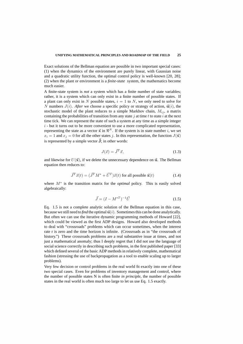
UNIFYING MATHEMATICAL PRINCIPLES AND ROADMAP OF THE FIELD 25
Exact solutions of the Bellman equation are possible in two important special cases:(1) when the dynamics of the environment are purely linear, with Gaussian noiseand a quadratic utility function, the optimal control policy is well-known [20, 28];(2) when the plant or environment is afinite-statesystem, the mathematics becomemuch easier.
A finite-state system isnot a system which has a finite number of state variables;rather, it is a system which can only exist in a finite number of possible states. Ifa plant can only exist inN possible states,i = 1 to N , we only need to solve forN numbersJ(i). After we choose a specific policy or strategy of action,~u(i), thestochastic model of the plant reduces to a simple Markhov chain,Mij , a matrixcontaining the probabilities of transition from any statej at timet to statei at the nexttime tick. We can represent the state of such a system at any time as a simple integeri - but it turns out to be more convenient to use a more complicated representation,representing the state as a vector~x in <N . If the system is in state numberi, we setxi = 1 andxj = 0 for all the other statesj. In this representation, the functionJ(~x)is represented by a simple vector~J; in other words:
J(~x) = ~JT ~x, (1.3)
and likewise forU(~x), if we delete the unnecessary dependence on~u. The Bellmanequation then reduces to:
~JT ~x(t) = ( ~JT M∗ + ~UT )~x(t) for all possible~x(t) (1.4)
whereM∗ is the transition matrix for theoptimal policy. This is easily solvedalgebraically:
~J = (I −M∗T )−1~U (1.5)
Eq. 1.5 is not a complete analytic solution of the Bellman equation in this case,because we still need tofindthe optimal~u(i). Sometimes this can be done analytically.But often we can use the iterative dynamic programming methods of Howard [22],which could be viewed as the first ADP designs. Howard also developed methodsto deal with “crossroads” problems which can occur sometimes, when the interestrate r is zero and the time horizon is infinite. (Crossroads as in “the crossroads ofhistory.”) These crossroads problems are a real substantive issue at times, and notjust a mathematical anomaly; thus I deeply regret that I did not use the language ofsocial science correctly in describing such problems, in the first published paper [33]which defined several of the basic ADP methods in relatively complete, mathematicalfashion (stressing the use of backpropagation as a tool to enable scaling up to largerproblems).
Very few decision or control problems in the real world fit exactly into one of thesetwo special cases. Even for problems of inventory management and control, wherethe number of possible states N is often finitein principle, the number of possiblestates in the real world is often much too large to let us use Eq. 1.5 exactly.

26 ADP: GOALS, OPPORTUNITIES AND PRINCIPLES
Early attempts to approximate dynamic programming were mostly based on a verysimple approximation to the Bellman equation. The true environment, howevercomplex, was approximated as a finite state system. For example, if the state vector~x is a bounded vector in<N , we can representJ(~x) by using a kind of N-dimensionallookup table containing all possible values of~x. But the size of such a lookup tablegrows exponentially withN ! This is the core of the “curse of dimensionality.”Warren Powell, in his chapter, discusses the curse of dimensionality in more detail.
Strictly speaking, ADP does not throw out that old approach to approximation! Ittreats it as a special case of one of thethree more general principles which are thecore of ADP:
(1) value approximation: Instead of solving forJ(~x) exactly, we can use auniversal approximation functionJ(~x,W ), containing a set of parametersW ,and try to estimate parametersW which makeJ(~x,W ) a good approximationto the true functionJ ;
(2) alternate starting points:Instead of always starting from the Bellman equationdirectly, we can start fromrelatedrecurrence equations (section 1.3.3.2) whichsometimes improve the approximation;
(3) hybrid design:We can combine multiple ADP systems and other systems inmore complex hybrid designs, without losing generality, in order to scale upto larger real-world problems, such as problems which involve multiple timescales and a mixture of continuous and discrete variables at multiple scales ofspace.
Dozens of different ADP designs or algorithms have been developed and used indifferent disciplines, based on one or more of these three general approaches. Inorder to build aunifiedADP design, which can learn to handle the broadest possiblevariety of complex tasks (as well as the mammalian brain does), we will need toexploit all three approaches to the utmost, and learn how to combine them togethermore effectively.
The remainder of this section will discuss each of these three approaches, in turn.It will proceed systematically from simpler ADP designs - easier to implement butless able to cope with difficult tasks - all the way up to the larger research challengescritical to the long-term strategic goals discussed above. In so doing, it will try toprovide a kind of global roadmap of this very complicated field.
1.3.3.1 Value Approximation and the Adaptive Critic This subsection willmainly discuss how we choose and tune an approximate value functionJ(~x,W )based on the Bellman equation proper. But the reader should be warned that thesimplest reinforcement learning packages based on this approach often convergeslowly when they are used on engineering tasks with a moderate number of contin-uous variables in them. Many critics of reinforcement learning have claimed thatreinforcement learning could not be useful on large-scale problems - mainly because

UNIFYING MATHEMATICAL PRINCIPLES AND ROADMAP OF THE FIELD 27
their students, using the easiest off-the-shelf tools in MatLab, were unable to tacklea large problem at first pass. The simplest designs are an important place to start, butone must build up beyond them (as in sections 1.3.2.2, 1.3.3.2 and even 1.3.3.3) inorder to handle larger problems. And of course we need further research and bettersoftware in order to capture the full power of the approach.
Even if we limit ourselves to ADP methods which tuneJ(~x,W ) based on the Bellmanequation proper, there is still a huge variety of more-or-less general designs. Thereare four decisions you must make when you put together such a system:
(1) What functionJ(~x,W ) do you choose to approximateJ(~x)?
(2) value updates:For anygivenstrategy or policy or controller~u(~x), how doyou adapt the weightsW to “best fit the Bellman equation”?
(3) policy updates:How do you represent and adapt~u(~x) itself as part of thisprocess?
(4) How do you coordinate, manage and time the value updates and policy updates?
With regard to question 1, many researchers still use lookup tables or linear basisfunction approximators:
J(~x,W ) =∑α
Wαfα(~x), (1.6)
where the functionsfα are preprogrammed basis functions or features chosen bythe user. A truly general-purpose computer program to calculate value updates andpolicy updates should be able to accommodate these particular choices as a specialcase. These special cases can also yield mathematical insights [25] which might beuseful as a stepping-stone to where we want to go. But our goal here is to get tothegeneralcase, where we need to be able to use a universal approximator able toapproximate "any" nonlinear function. Powell, in particular, has stressed that hissuccess in handling large problems is based on going beyond what he could get withlinear basis functions as in [25].
But which universal approximatorJ(~x,W ) do we use? The choice of functionapproximator has been one of the key issues explaining why some researchers havedone much better than others in real-world applications of ADP. We will also needto use approximators much more powerful than anyone has used in the past, in orderto scale up to more brain-like performance.
Universal approximation theorems have been proven for many, many systems such asTaylor series, fuzzy logic systems, wavelet systems, simple “global” neural networks(like the Multilayer Perceptron, MLP [7, 34]), and “local” neural networks like theRadial Basis Function (RBF), the CMAC, the SOM, the ART, etc. These all haveadvantages in various application domains. Some people from statistics argue thatthere can never be any real science here, because “there is no free lunch.” They arguethat some approximators will be better in some domains, and others will be better inothers, and there never can be a truly general-purpose system.
28 ADP: GOALS, OPPORTUNITIES AND PRINCIPLES
Certainly it makes sense for software designers to give their users a wide choice ofoptions - but the “no free lunch” theory misses a few critical points. It misses avery large historical literature on the foundations of induction and learning, which isrelevant here but is too complicated to discuss in detail. (e.g., see ([4], chapter 10)and sources cited in [34].) It misses the fact that approximators in family A can bedense in family B but not vice-versa. More concretely - it does not fully account forthe important, practical theorems proven by researchers like Barron [35] and Sontagon function approximation.
Taylor series, lookup tables, gain schedulers, CMAC and RBF are all examples ofthe broad class of linear basis function approximators. Barron [35] proved thatlinear basis function systems and MLPs are both universal approximators -but withdifferent accuracy in approximation. When we try to approximate smooth functions,and maintain a certain level of accuracy with more and more inputs (m), thenumberof parametersor nodes needed to maintain that accuracy rises at an exponentialrate with m, for linear basis function approximators, while it only rises as a gentlepolynomial function of m for MLPs. This makes intuitive sense, because we knowthat the required size of a lookup table grows exponentially with m, and we know thatother linear basis function approximators are based on the same underlying principle.
Barron’s result is only the tip of a very large iceberg, but it already conveys animportant lesson. In practical work in the neural network field, it is well-known thatMLPs allow greater accuracy in approximation formoderately largem than the localapproximators. (There are some exceptions, when the data is all clustered around afew points in state space, but that is not the general case.) A majority of the practicalsuccesses discussed in part II were based on using MLPs as the value approximator(s).On the other hand, it usually takes more time and skill to train MLPs than to trainlinear basis function approximators. Thus one has to work harder if one wants to getbetter results; this is a recurrent theme across all parts of the ADP field. There is alsostill a need for more research on ways to blend global networks like MLPs and localnetworks together, to combine the advantages of both,particularly when the speedof learning is an urgent issue; this is one of the subsystem-level issues I referred toin section 1.2.1.
I have speculated [36] that Elastic Fuzzy Logic systems (ELF) might be as powerfulas MLPs in function approximation, but for now this is just a speculation, so far as Iknow.
MLPs can do well in approximating smooth functions withm on the order of50−100.That is a huge step up from the old lookup-table dynamic programming.But it isstill a far cry from a brain-like scale of performance.It is good enough when thejob is to control a single car engine, or airplane, or turbogenerator or router. It isnotgood enoughto meet the needs of large-scale network control as discussed in part II.
Many people from AI and statistics have argued that we will never be able to scaleup to brain-like complexity, without exploiting a whole lot of prior information. Thisis true, in principle. But researchers going back to the philosopher Emmanuel Kantand the statistician Brad Efron have stressed that we can use a particulartypeof priorinformation which does not block our ability to learn new things in an open-minded

UNIFYING MATHEMATICAL PRINCIPLES AND ROADMAP OF THE FIELD 29
way. From a practical viewpoint - we can exploit tacit prior assumptions aboutsymmetry in order to design whole new classes of neural network designs, whichare capable of addressing large-scale network management, image processing andsegmentation and the like. There is a ladder of designs which now exists here, risingup from the generalized MLP [7, 34], to the Simultaneous Recurrent Network (SRN),to the Cellular SRN [37, 38], to the ObjectNet [39]. These should not be confusedwith the simple recurrent networks which are widely discussed in psychology but arenot so useful here.
A few quick comments about strategic games may be of interest to some readers.Fogel [18] has argued that the past success of reinforcement learning in playing gameshas been oversold. Reinforcement learning has generated human-class performancein backgammon and checkers,but onlywhen the programmers spent enormous effortin crafting the features they use in a linear basis function value function. There wasnever any true learning of the game from scratch. With tic-tac-toe, he was able totrain a perfect game player simply by using genetic algorithms to evolve an optimalgameplayer(~u(~x)). But this did not really work for checkers, as he had hoped. Hewasable to achieve human-level performance for the first time in checkers withoutcheating, by evolving a value-approximating MLP networkJ(~x,W ), and using thatnetwork as a basis for choosing moves. This was an historic achievement. But noone has ever achieved real human-level performance in the game of Go, with orwithout learning; based on what we learned from earlier work on lattices similar toGo boards [37], I would conjecture that: (1) Fogel’s approach might work with Go,if he replaced the MLP with a cellular SRN or ObjectNet; (2) even his earlier attemptto evolve a controller directly for checkers might have succeeded if he had used anSRN; (3) success in theater-like strategy games would also require Object Nets, butresearch on Go would be a good starting point to get there. I do not claim that thissimple approach would do full justice to the game of Go. Rather, it offers a tangiblehope to show that learning systems might outperform existing Go players. Onecould do better, to start, by using more advanced evolutionary computing methods,such as the use of particle swarm methods to adapt the continuous valued weightsin the value-approximating network. In parallel, we need to develop better gradient-exploiting methods to train recurrent recurrent systems like ObjectNets, in order totrain networks too large for evolutionary computing to handle, and in order to getcloser to brain-like approaches. Go can provide a testbed for even more powerfulgeneral concepts, but it would be useful to get this stream of research extended anddisseminated much further immediately, based on the best we can do today.
Again, this is all the tip of an iceberg, but the other three design questions above alsomerit serious discussion here.
First, the issue of how to do value updates.
Beginners to ADP often suggest that we should try to train the weights or parametersW by minimizing the following measure of error as a function ofW :
EG =∑
t
(J(~x(t),W )− (U(~x(t), ~u(t)) + γJ(~x(t + 1),W ))2, (1.7)
30 ADP: GOALS, OPPORTUNITIES AND PRINCIPLES
where the sum is taken over real or simulated pairs of data(~x(t), ~x(t + 1)). (Thesubscript “G” refers to Galerkin.) Years ago, I evaluated the performance of thisvalue-updating method, for the case of linear multiple-input multiple-output (MIMO)plants with nonzero noise. I proved that it converges to the wrong estimate of Walmost always [9, 40].
The connection to Galerkin is discussed at length in [9]. The procedure of minimizingEG is essentially a special case of one of the more general methods proposed byGalerkin decades ago to approximate the solution to partial differential equations(PDE). But the Bellman equation is not strictly a PDE, because of its stochasticaspect. The stochastic aspect turns out to be the source of the problem in tryingto apply Galerkin’s approach here[9]. More recently, Balakrishnan has adapted adifferent method of Galerkin (specialized to time-forwards systems rather than PDEin general) to the challenge of optimal, ADP control of systems like fluid flowsgoverned by PDE.
In 1977 [41], I proposed instead that we approximate Howard’s iterative proceduredirectly, bytraining the networkJ(~x,W ) to try to match or predict the targets:
J∗(t) = U(t) + J(t + 1)/(1 + r), (1.8)
This training could be done by minimizing least square error and backpropagation,or we could useany othermethod used to train any kind of function approximatorto match examples of input vectors and desired output vectors. I called this method“Heuristic Dynamic Programming” (HDP) [41]. This statement of the method isquite brief - but it is complete. The method really is quite simple, in the general case.(See [3] for elaborate discussions of how to embed this idea in simple, general formwithin a larger software system for ADP.)
Earlier, in 1973 [42], Widrow implemented an alternative training method for a neuralnetwork which he called a “critic”, for use in playing blackjack. In effect, he trainedJ(~x(t),W ) directly to predict:
J∗(t) =T−1∑τ=t
U(τ) + U∗(T ), (1.9)
whereU∗ is a kind of terminal payoff at a terminal timeT . There was no connectionmade to utility functions or dynamic programming. In 1983, Barto, Sutton andAnderson [26] generalized Widrow’s method to define the class of methodsTD(λ),such thatλ = 0 andλ = 1 would yield a choice between Eq. 1.8 and Eq. 1.9. Therewas no indication of a connection to [41] or to any form of dynamic programmingat that time; that connection was made later, in 1987, when Sutton read [43], andset up the discussions at GTE which later led to the 1988 NSF workshop reportedin [2]. Since then, we have used the term “critic” or “critic network” to refer toany parameterized network used to approximateJ(~x) or to approximateany of theother various value functions which emerge from relatives of the Bellman equation(section 1.3.3.2). An "adaptive critic" system is any system which contains such a

UNIFYING MATHEMATICAL PRINCIPLES AND ROADMAP OF THE FIELD 31
critic network, plus some mechanism to adapt or tune the critic based on off-linelearning or on-line learning,
Many researchers such as Williams have been able to show how pathological trainingsets~x can cause HDP itself to converge to the wrong answer or even to diverge. VanRoy [44] has proven that it will always converge to the right value, under reasonableconditions,if the training set is chosen from the normal stream of experience onewould expect to see while controlling and observing the actual plant. There areseveral more complex variants of HDP, for which I have proven that the methodwill always converge to the right value function for linear MIMO plants (includingstochastic versions), even when the training sets are chosen in a pathological manner[9]. There are also a wide variety of other methods available, some more trulylearning-based and some based on linear programming, as described by Van Roy’schapter in this book. It would be interesting to see whether Van Roy’s approach couldbe made more powerful, by exploiting the nonlinear programming methods describedin Momoh’s chapter. It would also be interesting to see whether such methods couldbe restructured or adapted into true, scaleable learning-based methods for adaptingJ(~x,W ), similar in spirit to some of the work by Trafalis in training simpler typesof neural networks based on sophisticated ideas from operations research[45].
Policy updates are much more straightforward than value updates, in theory. Manyresearchers in AI address tasks where there is only a finite set of possible actionsto take at any time t. In designing a system to play Go, for example, one mightsearch over every possible move, and do the maximization on the fly by brute force.(There are many other similar choices familiar to AI researchers.) In engineeringapplications today, it is reasonable to train a controller~u(~x,Wu), which may alsobe a universal approximator. For example, we may train the weightsWuα so as tomaximize <U(t)+γJ(t+1)>, by adapting them in response to a stochastic gradientestimate:
∂∂Wuα
(U(t) + J(t+1)
1+r
)
≈ ∑i
((∂U
∂ui(t)+ γ
∑j
∂J(t+1)∂xj(t+1) ·
∂xj(t+1)∂ui(t)
)· ∂ui(t)
∂Wuα
)(1.10)
The control theorist should immediately see that this isexactly the same as theprocedure used to update or train a controller in Indirect Adaptive Control (IAC)[46], except that IAC eliminates “U ” and it replacesJ(t + 1) with a fixedmeasureof tracking error which is basically arbitrary. Both here and in IAC, we must train orobtain a model of the plant in order to estimate the required partial derivatives. In bothcases, the derivative calculations and summation can be done more quickly and moreefficiently in real time by using an algorithm which I call “backpropagation through amodel.” [3, 7]. This algorithm calculates the required derivatives efficiently throughany differentiable model, neural, fuzzy, classical or other. In 1988 [2], I coinedthe term “Backpropagated Adaptive Critic” (BAC) [2] to name this way of traininga controller or Action Netu(~x,Wu). The stability guarantees for IAC depend onhighly restrictive assumptions, even in the linear case [21]; however, there is good
32 ADP: GOALS, OPPORTUNITIES AND PRINCIPLES
reason to believe that theextensionof IAC provided by the use of new HDP variantscan yield universal total system stability guarantees forall controllable linear plants[9].
More recently, some researchers have used the term “Policy Gradient Control Syn-thesis” (PGCS) for this approach to updating or training an Action Net. In certaindesigns, this may require the efficient real-time calculation of selected second deriva-tives. The form of second-order backpropagation required for such applications wasfirst discussed in 1979 [33], but explained in more detail in [3].
High-level decision problems sometimes require more than just brute-force maxi-mization or an Action network of this type. As we scale up to brain-like capabilities,we will need to design and train something like Option Networks, which generatereasonablechoicesfor ~u(t) decisions, along with search and selection systems to gowith them.[47]. This involves some kind of stochastic search capability, related toevolutionary computing (EC), but not at all the same. In conventional EC, the usersupplies a functionU(~u), and a fixed algorithm searches through possible values of~u. But in brain-like stochastic search (BLiSS?), we try to develop learning systemswhich learn to do better and better stochastic search forfamiliesof optimization prob-lemsU(~u, ~x). For example, one such functionU(~u, ~x) would be thefamily of alltravelling salesman problems for 1,000 cities, where x is the vector of coordinates ofthose cities. There has been some preliminary research related to BLiSS by Wunschand by Serpen, but much more will be needed.
Finally, the issue of how to manage, time and control value updates and policy updatesis an extremely complex issue, very dependent on the specific choices one makes.Many chapters in this book will discuss various aspects of these issues. As a generalrule, we do know that mammal brains somehow do concurrent real-time updates ofalltheir components. But they also need periods of offline-learning and consolidation,in deep sleep and dreams. There are learning tasks in ADP which clearly relate tothese biological functions [1, 2, 43], but more research will be needed to pin themdown more completely.
1.3.3.2 Alternative Starting Points: Beyond the Bellman Equation ProperTheprevious section discussed value approximation for ADP designs baseddirectly onthe Bellman equation - HDP, TD and variations of them. The Bellman equation itselfmay be viewed as a kind of recursion equation for the functionJ(~x).There are two alternative starting points which are important to applications ofADP today. One of them is the recursion equation which underlies methods calledAction-Dependent HDP (ADHDP), Q learning, and related methods. The other isthe recursion relation underlying Dual Heuristic Programming (DHP); that equationis essentially a stochastic generalization of the Pontryagin equation, which is asimportant and well-known as the Hamilton-Jacobi equation in some fields of science.
Crudely speaking, the ADHDP/Q recurrence leads to ADP designs which do notdirectly require a model of the plant or environment. (However, they do not escapethe issues discussed in section 1.3.3.2.) The DHP recurrence equation was developed

UNIFYING MATHEMATICAL PRINCIPLES AND ROADMAP OF THE FIELD 33
in order to overcome scaling problems with all methods discussed so far in thissection, for tasks involving continuous variables.
Q learning and ADHDP are different methods, dating back to two independentsources in 1989 - the classic PhD thesis of Watkins [23] and a far briefer paper givenat the IEEE Conference on Decision and Control [24], respectively. But both can bederived from the same recurrence equation. Here I will derive that equation as in[24], but will now label the new value function as “Q” instead of “J .”
If we write the Bellman equation as:
J(~x(t)) = max~u(t)
< U(~x(t), ~u(t)) + γJ(~x(t + 1)) >, (1.11)
we may simplydefine:
Q(~x(t), ~u(t)) =< U(~x(t), ~u(t)) + γJ(~x(t + 1)) > . (1.12)
Using this definition, Eq. 1.11 may be expressed equivalently as :
J(~x(t)) = max~u(t)
Q(~x(t), ~u(t)), (1.13)
Substituting Eq. 1.13 into Eq. 1.12, we deduce :
Q(~x(t), ~u(t)) =< U(~x(t), ~u(t)) + γ max~u(t+1)
Q(~x(t + 1), ~u(t + 1)) > (1.14)
Eq. 1.14 is the recurrence equation underlying both ADHDP and Q-learning.
Q learning generally uses lookup tables to represent or approximate the functionQ.In the 1990 workshop which led to [3], Watkins did report an effort to approximateQ using a standard CMAC neural network, for a broom-balancing task; however, hereported that that variation did not work.
With Q learning, as in TD learning, one can derive the policy~u(~x) simply by con-sidering every possible choice of actions, in tasks where there is only a manageable,finite list of choices. However, in the TD case, dynamic programming clearly callson us to try topredict< J(t + 1) > for each choice, which then requires some kindof model of the plant or environment. With Q learning, you only need to know theQfunction. You escape the need for a model. On the other hand, if~x and~u are actuallycontinuous variables, and if you are using a lookup table approximation toQ, thenthe curse of dimensionality here is even worse than with conventional DP.
For Action-Dependent HDP (ADHDP) [3, 24], I proposed that we approximateQ(~x(t), ~u(t)) and~u(~x) by using universal approximators, like neural networks. Wecan train a networkQ(~x, ~u,W ) to try to match targetsQ∗ based on the recurrenceEq. 1.14, usingexactlythe same procedure as in HDP. (See [3] for pseudo-code,flowcharts, examples and analysis.) We can train~u(~x,Wu) to maximizeQ, by tuning

34 ADP: GOALS, OPPORTUNITIES AND PRINCIPLES
the weights ofWu in response to the derivatives ofQ, backpropagated fromQ to ~uto the weights.
Some neural network researchers would immediately ask: “Doesn’t the use of back-propagation lead to slow learning here?” Not necessarily. When a traditional MLP istrained by backpropagation, the learning is indeed slower than what we see with radialbasis functions (RBF), for example. But the problem lies with the MLP structure,more than with backpropagation. (It is also important to know modern techniquesfor adjusting learning rates and such.) More powerful function approximators (likehumans!) are even trickier to train, because they are searching a space of possibili-ties which is even larger. But when backpropagation is used to train simpler, localnetworks, it can be reasonably fast.
As an example, David White - co-sponsor of the 1990 joint NSF/McDonnell-Douglasworkshop which led to [3] - applied ADHDP in 1990 to control the McDonnell modelof the F-15 aircraft in simulation. He and Urnes did a study in which the simulatedaircraft was badly damaged in random ways, and the ADHDP system tried to relearnthe control fast enough (2 seconds) to keep the craft from crashing. It succeeded abouthalf the time, which was far better than conventional methods (2 percent survival orso). The neural networks used to approximateQ and~u were a new, differentiablevariant of the CMAC design. (See [3] for details.) White and Sofge also usedADHDP to produce high-quality carbon-carbon parts using a cost-effective processwhich had defied earlier, expensive approaches based on more traditional methods.(See [3] - and section 1.2 of this chapter.)
ADHDP in some form has been independently rediscovered by a number of re-searchers, who have reported good results. For example, Ford Research [48] reporteda quick and easy solution of the bioreactor control challenge problem in [3], which,according to Ungar, defied the very best and most modern adaptive control methods.Many of Si’s results reported in this book use a design in this category. Shibata’s“fuzzy critic” for robot control [49], developed under Fukuda, also appears to be inthis category. It is good news that we are beginning to integrate and consolidate moreof this work.
ADHDP can handle larger-scale engineering problems than lookup-table Q or TDapproaches. (From an engineering viewpoint, I have described the lookup-table and“associative trace” versions of Q and TD as “level 1,” versus ADHDP as “level 2.”)But it still encounters problems as one tries to scale up to even larger problems, andit also has problems related to “persistence of excitation” ([3], chapter 13). Becauseof these issues, and because of the issues of partial observability, I have argued thatthe combination of HDP and BAC discussed in the previous section tends to be morepowerful - “level 3” - on engineering problems which involve continuous variables.In order to scale up still further - “level 4” - many of us have gone on to use a differentrecurrence equation altogether, the DHP recurrence equation.
The correct recurrence equation for DHP may be derived in a straightforward way,by first defining:
~λ(t) = ∇~xJ(~x(t)), (1.15)

UNIFYING MATHEMATICAL PRINCIPLES AND ROADMAP OF THE FIELD 35
which is another way of writing:
λi(t) =∂J(~x(t))∂xi(t)
(∀i), (1.16)
by performing the calculation for a particular policy~u(~x), and by differentiating Eq.1.11 with respect toxi(t) to get:
λi(t) =
⟨∂U(~x(t),~u(t))
∂xi+ γ
∑j
∂J(~x(t+1))∂xj(t+1) · ∂xj(t+1)
∂xi(t)
+∑k
(∂U(~x(t),~u(t))
∂uk(t) + γ∑j
∂J(~x(t+1)∂xj(t+1) ·
∂xj(t+1)∂uk(t)
)· ∂uk(~x(t))
∂xi(t)
⟩ (1.17)
This general type of complex derivative calculation relies heavily on mathematicalfoundations discussed further in [6].
Some control theorists have asked at first: “Can you do this? Just differentiate theBellman equation?” In fact, weknowthat Eq. 1.11 must hold for the optimal policy.So long asJ andu and the plant are differentiable (within the Kolmogorov probabilityformalism [10]), we know that Eq. 1.17must holdas well, for an optimal policy. Itis a necessary condition for an optimum. Likewise, the policy update equivalent toEq. 1.10 is trivial to deduce. (See [3].) But Eq. 1.10 is not asufficientconditionfor a globally optimal policy; that is why I discussed stochastic search issues afterthe discussion of Eq. 1.10, and similar issues apply here. For complex nonlinearproblems in general it is often possible to guarantee local optima, superiority to linearmethods, and global optima in various convex cases in a rigorous way, but intelligentsystems design can never guarantee “perfect” creativity in finding global optima.Stronger guarantees exist for GDHP (to be discussed below) than for DHP.
The recurrence equation for~λ follows by using the definition of~λ to simplify Eq.1.17:
λi(t) =
⟨∂U∂xi
+ γ∑j
λj(t + 1) · ∂xj(t+1)∂xi
+∑k
(∂U∂uk
+ γ∑j
λj(t + 1) · ∂xj(t+1)∂uk
)· ∂uk
∂xi
⟩ (1.18)
where variables without time arguments refer to values at timet.
The obvious way to approximate this recurrence relationship is to train an approxi-mator,~λ(~x,W ), to meet the targets~λ∗ defined by the right-hand side of Eq. 1.18;more precisely, starting from any estimate ofW , one can update the estimate ofW tomake~λ(~x,W ) better match~λ∗(~x, W ), where~λ∗(~x, W ) is defined by the right-handside of Eq. 1.18, using thecurrentestimates ofW to estimate the values of~λ(t + 1)by ~λ(~x(t + 1), W ) as required to calculate to right-hand side of Eq. 1.18. Details,flow-charts, pseudo-code and some theoretical analysis (along with a couple of un-

36 ADP: GOALS, OPPORTUNITIES AND PRINCIPLES
fortunate typos) can be found in [3], chapter 13. Using modular code design, and abasic understanding of backpropagation, it is not necessary to be an expert in controltheory or on these equations in order to implement DHP.
Certain warnings are needed here. Although I discussed the general idea of DHPback in 1977 [41], I did not really specify the method then (unlike the case forHDP). In 1981 [50]. I discussed a way to implement the idea, using backpropagationand an error function similar to Eq. 1.7; however, that kind of variation (which Inow call DHPG) converges to the wrong answer almost always for linear dynamicalsystems with noise [9]. In order to converge to the correct answer, it is necessaryin principle to include the (∂uk/∂xi) terms, which were explained for the first timein [3]. (See [9] for extensions important to robust and adaptive control.) All of theactual implementations and applications of DHP occurred after the publication of[3]. Many of the most important ones appear in this book.
The vector~λ of DHP has many connections to concepts in other fields of science andengineering. For example, to the economist,λi(t) represents a kind of “marginalutility” or “shadow price” - the long-term market value of the commodity whosequantity or level is given by the variablexi. DHP critics could actually be usedas pricing systems. In the Pontryagin equation,λi is called a “costate variable;” inmodern optimal control [20, 28], the letter “λ” is still used for costate variables. Thevector~λ is also closely related to the gradients calculated in backpropagation throughtime, which creates many opportunities for seamless, integrated hybrid designs,discussed in part in the Chapter by Prokhorov.
DHP could have some interesting applications in network control, as discussed insection 1.2.2. For a large network system, we would need something like an ObjectNet(section 1.3.3.1) in order to input observations across anentire electric power grid,and output a vector of shadow prices or values for all of those observed values.Physically, an ObjectNet may be thought of as a specific kind of highly coordinatedassembly ofcomponentnetworks, each of which refers to a particular object in thegrid; thus we could choose to implement such a value-approximation network as adistributed system, with chips located near each object to implement the componentnetwork for that object. Such a system would output the estimate of values whichapply to each object, from the node which is actually located at that object. Ateach object, we could perform a kind of local optimization over time, using a lower-level ADP system which responds to these global values, using a master-slave kindof arrangement similar to the one discussed in section 1.3.2.2. Communicationconstraints could simply be represented as part of the topology specification of theObjectNet to be trained.
DHP is not the only method in its class. There have also been a few simulations ofAction-Dependent DHP (ADDHP), Globalized DHP (GDHP), ADGDHP and relatedError Critic designs. (See [3, 9] and some of the work of Wunsch and Prokhorov.) Inessence, GDHP is a hybrid of HDP and DHP. It trains a scalar critic which estimatestheJ function, but uses second derivatives in order to achieve the same effect as DHP.In effect, GDHP provides a way of performing DHP (as described above) while alsoguaranteeing strict adherence to the requirement that the vectors~λ are the gradient of
UNIFYING MATHEMATICAL PRINCIPLES AND ROADMAP OF THE FIELD 37
a functionJ . More generally [43], GDHP allows one to train the critic to minimizea weighted sum of the DHP second-order error measure and the usual HDP/TD first-order error measure; ifsomestate variables are continuous while others are discrete,one can use GDHP on the entireJ function by simply by not using the (undefined)second-order terms for the discrete state variables. (The discussion of [43] needs tobe updated, to reflect the convergence results in [3] and [9].) Benchmark studies byWunsch and Prokhorov show little difference in performance between the easier DHPmethod and GDHP in difficult engineering problems involving continuous variables.Thus it may be premature to say more about GDHP at the present time.
1.3.3.3 Hybrid and Large-Scale Designs: Closing the Gap to the Mammal BrainLevel This chapter started out by posing a question: when and how can we handledynamic optimization problems as large and as complex as what the smallest mammalbrain can learn to handle? (Of course, such systems could do far better than mice orhumans onsome problems, as a byproduct of this effort.)
Years ago, I believed that the kinds of designs discussed in sections 1.3.3.1 and1.3.3.2 might be enough to achieve that goal by themselves. After all, the famousneuropsychologist Hebb argued decades ago that all the complexities of higher-orderintelligence might result as anemergent propertyof a much simpler kind of learningsystem [51]. Why could they not emerge from these kinds of more sophisticated andpowerful learning design? The parallels to what was known about the brain in 1980were also quite strong [43].
Recent research both in neuroscience and in technology has made it ever more clearthat our earlier beliefs were mistaken.
For example, neuroscience has learned a great deal about thebasal ganglia[52, 53].Decision-making in the brain does not follow the highly rigid, pre-programmed kindsof hierarchies that were used in classical AI and in the old Red Army - but it clearlydoes have a mechanism for exploitingmultiple time scales. Furthermore, it nowseems more and more clear that critic methods canconverge faster- by orders ofmagnitude at times - when they include a way to exploit such structure. The challengelies in how to build systems which exploit such properties as effectively as possible,without using ad hoc patches and hierarchies that interfere with the flexibility oflearning and the ability to converge in the end to a true multi-level optimum.
Three strands of research have demonstrated promising ideas to help us handle thisissue. The field ofhybrid control, represented here by Shankar Shastry, has studieddecoupled methods for the HJB equation, particularly for problems involving a mix ofcontinuous an discrete variables. AI researchers in reinforcement learning have alsoexplored a number of ideas; the chapter by Dietterich gives an excellent overview,and the chapter by Barto describes further recent work. I myself have also developedsome modified multilevel Bellman equations [47, 54] based on the concept of fuzzyor crisp partitions of the state space, which may have some role to play in this strandof research. (These were inspired in part by some earlier work by Sutton [55], and bysome work on matrix decomposition theory which I did in 1978, but go substantiallybeyond the initial inspirations.)

38 ADP: GOALS, OPPORTUNITIES AND PRINCIPLES
Spatial structure is also very critical, as was already discussed in section 1.3.3.1.Large-scale network control will be an important testbed in learning how to handlespatial structure, but concepts like the Object Net still leave open some key questions.For example, how do brainslearn object types? How can systems like the brainimplement such structures, using some kind of multiplexing or thalamic gating [56]?How does spatial complexity interface with temporal complexity?
As we move up to systems which truly make high-level decisions, in order to managemultiple levels of time, issues related to stochastic search and stochastic systemidentification become ever more important. This chapter has already discussed theseissues - but we need to remember that they will become more important in the future.
None of this work would allow us to build an artificial human mind. Thehumanmindinvolves a whole new set of issues [1] far beyond the scope of this chapter. But99 percent of the human brain is more or less equivalent to structures which exist inthe smallest mouse. A deeper, more functional understanding of the latter should bea big step forward, inallowingus someday to understand the former more deeply aswell.

Bibliography
1. P. Werbos, “What do neural nets and quantum theory tell us about mind andreality,” In K. Yasue, M. Jibu & T. Della Senta (eds),No Matter, Never Mind :Proceedings of Toward a Science of Consciousness : Fundamental Approaches(Tokyo ’99), John Benjamins Pub Co, 2002. See also P.Werbos, “Optimization: AFoundation for understanding consciousness,” In D.Levine & W. Elsberry (eds),Optimality in Biological and Artificial Networks,Erlbaum, 1997.
2. W.T. Miller, R. Sutton & P. Werbos (eds),Neural Networks for Control, MITPress, 1990, now in paper.
3. White & D. Sofge (eds),Handbook of Intelligent Control, Van Nostrand, 1992.
4. P. Werbos, Neurocontrollers, in J. Webster (eds),Encyclopedia of Electrical andElectronics Engineering, Wiley, 1999.
5. M. Hoffert et al, “Advanced Technology Paths to Global Climate Stability:Energy For a Greenhouse Planet,”Science, Nov. 1, 2002.
6. P. Werbos,Beyond Regression: New Tools for Prediction and Analysis in the Be-havioral Sciences, Ph.D. Thesis, Committee on Applied Mathematics, HarvardU., 1974. Reprinted in its entirety in P.Werbos,The Roots of Backpropagation:From Ordered Derivatives to Neural Networks and Political Forecasting, Wiley,1994.
7. P. Werbos, “Backpropagation through time: what it does and how to do it,”Proc.IEEE, Vol. 78, No. 10, October 1990. Updated version reprinted as chapter 8 of[6].
8. J.A. Suykens, B.DeMoor and J.Vandewalle, “Nlq theory: a neural control frame-work with global asymptotic stability criteria,”Neural Networks, Vol. 10, No.4,p.615-637, 1997.
9. P. Werbos,Stable Adaptive Control Using New Critic Designs. ArXiv.org: adap-org/9810001 (1998)
10. Jacobson/Mayne D.Jacobson & D.Mayne,Differential Dynamic Programming,American Elsevier, 1970.
39
40 BIBLIOGRAPHY
11. P. He and J. Sarangapani, “Neuro Emission Controller for Minimizing CyclicDispersion in Spark Ignition Engines,” TNN submitted, 2003. Condensed ver-sions are in press in IJCNN 2003 Proceedings (IEEE) and CCA 2003 Proceedings(IEEE).
12. F. Lewis, J. Campos and R. Selmic,Neuro-Fuzzy Control of Industrial Systemswith Actuator Nonlinearities, Philadellphia: SIAM, 2002.
13. E.A. Feigenbaum and J. Feldman,Computers and Thought, McGraw-Hill, 1963.
14. J. Von Neumann and O. Morgenstern,The Theory of Games and EconomicBehavior, Princeton NJ: Princeton U. Press, 1953.
15. H. Raiffa,Decision Analysis, Addison-Wesley, 1968.
16. P. Werbos, “Rational approaches to identifying policy objectives,”Energy: TheInternational Journal, 15 (3/4), 1990, p.171-185.
17. D.F. Walls and G.F. Milburn,Quantum Optics, Springer, New York, 1994.
18. David B. Fogel,Blondie24: Playing at the Edge of AI, Morgan-Kauffman, 2001.
19. T. Landelius,Reinforcement Learning and Distributed Local Model Synthesis,Ph.D. thesis and Report No.469, Department of Electrical Engineering, Linkop-ing U., 58183, Linkoping, Sweden.
20. Robert F. Stengel,Optimal Control and Estimation, Dover edition, 1994.
21. K. Narendra and A. Annaswamy,Stable Adaptive Systems, Englewood NJ:Prentice-Hall, 1989; Washington D.C.: Hemisphere, 1982.
22. R. Howard,Dynamic Programming and Markhov Processes, MIT Press, 1960.
23. C.J.C.H. Watkins,Learning From Delayed Rewards, Ph.D. thesis, Universityof Cambridge, England, 1989. See also Watkins and Dayan, “Technical note:Q-learning,”Machine Learning, Vol. 8, No.3/4, 1992, p.279-292.
24. P. Werbos, “Neural networks for control and system identification,”IEEE Proc.CDC89, IEEE, 1989.
25. D.P. Bertsekas and J.N. Tsisiklis,Neuro-Dynamic Programming, Athena Scien-tific, 1996.
26. A. Barto, R. Sutton and C. Anderson, “Neuronlike adaptive elements that cansolve difficult learning control problems,”IEEE Trans. SMC, Vol. 13, No.5,1983, p.834-846.
27. P. Werbos, “The elements of intelligence,”Cybernetica (Namur), No.3, 1968.
28. A. Bryson & Y.C. Ho,Applied Optimal Control, Ginn, 1969.

BIBLIOGRAPHY 41
29. J.S. Baras and N.S. Patel, “Information state for robust control of set-valueddiscrete time systems,”Proc. 34th Conf. Decision and Control (CDC), IEEE,1995. p.2302.
30. S. Mukhopadhyay and B. Jain, “Multi-agent Markhov decision processes withlimited agent communication,”Proc. Of the Int’l Joint Conf. On Control Appli-cations and Int’l Symposium on Intelligent Control (IEEE CCA/ISIC01), IEEE:200l.
31. T. Kohonen,Self-Organizing Maps, New York: Spinger, 1997, Second Edition.Also see H.Ritter, T.Martinetz, and K.Schulten,Neural Computation and Self-Organizing Maps, Addison-Wesley, 1992.
32. J. Albus, “Outline of Intelligence,”IEEE Trans. Systems, Man and Cybernetics,Vol.21, No.2, 1991.
33. P. Werbos, “Changes in global policy analysis procedures suggested by newmethods of optimization,”Policy Analysis and Information Systems, Vol.3, No.1,June 1979.
34. P. Werbos, Backpropagation: General Principles and Issues for Biology. In D.Fogel and C. Robinson (eds), Computational Intelligence: The Experts Speak.IEEE, 2003.
35. A.R. Barron, “Universal approximation bounds for superpositions of a sigmoidalfunction,” IEEE Trans. Info. Theory, 39(3) 930-945, 1993.
36. P. Werbos, “Elastic fuzzy logic: a better fit to neurocontrol and true intelligence,”J. Intelligent & Fuzzy Systems, Vol. 1, No.4, 1993.
37. X.Z. Pang & P. Werbos, “Neural network design for J function approximationin dynamic programming,”Math. Modelling and Scientific Computing, Vol.5, NO.2/3, 1996 (physically 1998). Available also as adap-org/ 9806001 atarXiv.org. See also P.Werbos & X.Z.Pang, “Generalized maze navigation: SRNcritics solve what feedforward or Hebbian nets cannot,”Proc. Conf. Systems,Man and Cybernetics (SMC), Beijing, IEEE, 1996.
38. T. Yang & L.O. Chua, “Implementing Back-Propagation-Through-Time Learn-ing Algorithm Using Cellular Neural Networks,”Int’l J. Bifurcation and Chaos,Vol. 9, No. 9, June 1999, p.1041-1074.
39. See P. Werbos posted at www.iamcm.org, and [47].
40. P. Werbos, “Consistency of HDP applied to a simple reinforcement learningproblem,”Neural Networks, March 1990.
41. P. Werbos, “Advanced forecasting for global crisis warning and models of intel-ligence,”General Systems Yearbook, 1977 issue.

42 BIBLIOGRAPHY
42. B. Widrow, N. Gupta & S. Maitra, “Punish/reward: learning with a Critic inadaptive threshold systems,”IEEE Trans. SMC, 1973, Vol. 5, p.455-465.
43. P. Werbos, “Building and understanding adaptive systems: A statisti-cal/numerical approach to factory automation and brain research,”IEEE Trans.SMC, Jan./Feb. 1987.
44. J. Tsitsiklis & B. Van Roy, “An analysis of temporal-difference learning withfunction approximation,”IEEE Trans. Auto. Control, Vol. 42, No. 5, May 1997.
45. T.B. Trafalis and S. Kasap, “Artificial neural networks in optimization and ap-plications,” Handbook of Applied Optimization, P. M. Pardalos and M. G. C.Resende (eds), Cambridge University Press 2000.
46. K. Narendra & S. Mukhopadhyay, “Intelligent control using neural networks,”In M. Gupta & N. Sinha (eds),Intelligent Control Systems, IEEE Press, 1996.
47. P. Werbos, “A Brain-Like Design To Learn Optimal Decision Strategies in Com-plex Environments,” in M.Karny, K.Warwick and V.Kurkova (eds),Dealingwith Complexity: A Neural Networks Approach, Springer, London, 1998. Alsoin S.Amari and N.Kasabov,Brain-Like Computing and Intelligent InformationSystems, Springer,1998.
48. F. Yuan, L. Feldkamp, G. Puskorius & L. Davis, “A simple solution to the biore-actor benchmark problem by application of Q-learning,”Proc. World Congresson Neural Networks, Erlbaum, 1995.
49. T. Shibata,Hierarchical Intelligent Control of Robotic Motion, Master’s Thesis,Dept. of Electronic Mechanical Engineering, Nagoya University, Japan, 1992,chapter 5.
50. P. Werbos, “Applications of advances in nonlinear sensitivity analysis,” inR.Drenick & F. Kozin (eds),System Modeling and Optimization: Proc. IFIPConf. (1981), Springer 1982; reprinted as chapter 7 in [6].
51. D.O. Hebb,The Organization of Behavior, Wiley, 1949.
52. James C. Houk, J.L. Davis and D.G. Beiser (eds),Models of Information Pro-cessing in the Basal Ganglia, Cambridge, Mass.: MIT Press, 1995.
53. Karl H. Pribram, ed.,Brain and Values, Erlbaum: Hillsdale, NJ, 1998. (See alsoearlier books edited by Pribram in the same series from Eerlbaum.)
54. P. Werbos, “Multiple Models for Approximate Dynamic Programming and TrueIntelligent Control: Why and How,” In K. Narendra, (eds),Proc. 10th Yale Conf.on Learning and Adaptive Systems, New Haven: K.Narendra, EE Dept., YaleU., 1998.
55. R. Sutton, “TD Models: Modeling the World at a Mixture of Time Scales,”CMPSCI Technical Report, 95-114, U.Mass. Amherst, December 1995, later

BIBLIOGRAPHY 43
published inProc. 12th Int. Conf. Macjine Learning, 531-539, Morgan Kauf-mann, 1995.
56. Charles H. Anderson, B. Olshausen and D. Van Essen, “Routing networks invisual cortex,” In M. Arbib (eds),The Handbook of Brain Theory and NeuralNetworks, MIT Press, 1995, First Edition, p. 823-826.


Part I
Overview


2 Reinforcement Learning and itsRelationship to SupervisedLearning
ANDREW G. BARTO and THOMAS G. DIETTERICHUniversity of Massachusetts Oregon State University
Editor’s Summary: This chapter focuses on presenting some key concepts ofmachine learning, approximate dynamic programming, and the relationships betweenthem. Discussion and comparisons are made based on various aspects of the two fieldssuch as training information, behavioral variety, problem conversion, applicable tasks,etc. The chapter contains many real-world examples and applications to illustratethe use of these concepts. The primary focus of this chapter is a discussion ofthe concepts and strategies of machine learning, not necessarily algorithmic details.This chapter provides high-level perspective on machine learning and approximatedynamic programming.
2.1 INTRODUCTION
The modern study of approximate dynamic programming (DP) combines ideas fromseveral research traditions. Among these is the field of Artificial Intelligence, whoseearliest period focussed on creating artificial learning systems. Today, MachineLearning is an active branch of Artificial Intelligence (although it includes researchersfrom many other disciplines as well) devoted to continuing the development ofartificial learning systems. Some of the problems studied in Machine Learningconcern stochastic sequential decision processes, and some approaches to solvingthem are based on DP. These problems and algorithms fall under the general headingof reinforcement learning. In this chapter, we discuss stochastic sequential decisionprocesses from the perspective of Machine Learning, focussing on reinforcementlearning and its relationship to the more commmonly studied supervised learningproblems.
47

48 RL AND ITS RELATIONSHIP TO SUPERVISED LEARNING
Machine Learning is the study of methods for constructing and improving softwaresystems by analyzing examples of their behavior rather than by directly program-ming them. Machine Learning methods are appropriate in application settings wherepeople are unable to provide precise specifications for desired program behavior, butwhere examples of desired behavior are available, or where it is possible to assign ameasure of goodness to examples of behavior. Such situations include optical char-acter recognition, handwriting recognition, speech recognition, automated steeringof automobiles, and robot control and navigation. A key property of tasks in whichexamples of desired behavior are available is that people can perform them quiteeasily, but people cannot articulate exactlyhow they perform them. Hence, peoplecan provide input-output examples, but they cannot provide precise specifications oralgorithms. Other tasks have the property that people donot know how to performthem (or a few people can perform them only with great difficulty), but people areable to evaluate attempts to perform them, that is, to score behavior according tosome performance criterion. Situations like this include playing master-level chessand controlling the nation-wide power grid in an efficient and fail-safe manner.
Machine Learning methods are also appropriate for situations where the task ischanging with time or across different users, so that a programmer cannot anticipateexactly how the program should behave. For example, Machine Learning methodshave been applied to assess credit-card risk, to filter news articles, to refine infor-mation retrieval queries, and to predict user browsing behavior in computer-basedinformation systems such as the world-wide web.
Another area of application for Machine Learning algorithms is to the problemof finding interesting patterns in databases, sometimes calleddata mining. Manycorporations gather information about the purchases of customers, the claims filedby medical providers, the insurance claims filed by drivers, the maintenance recordsof aircraft, and so forth. Machine Learning algorithms (and also, many traditionalmethods from statistics) can find important patterns in these data that can be appliedto improve marketing, detect fraud, and predict future problems.
We begin by describing tasks in which examples of desired behavior are available.
2.2 SUPERVISED LEARNING
In supervised learning, the learner is giventraining examplesof the form(xi, yi),where each input valuexi is usually ann-dimensional vector and each output valueyi
is a scalar (either a discrete-valued quantity or a real-valued quantity). It is assumedthat the input values are drawn from some fixed probability distributionD(x) andthen the output valuesyi are assigned to them. The output values may be assigned bya fixed functionf , so thatyi = f(xi), or they may be assigned stochastically by firstcomputingf(xi) and then probabilistically perturbing this value with some randomnoise. This later, stochastic view is appropriate when the output values are assignedby a noisy process (e.g., a human judge who makes occasional errors). In either case,

SUPERVISED LEARNING 49
the goal is to correctly predict the output values of new data pointsx drawn from thesame distributionD(x).For example, in optical character recognition, each input valuexi might be a 256-bitvector giving the pixel values of an8×8 input image, and each output valueyi mightbe one of the 95 printable ascii characters. When, as in this case, the output valuesare discrete,f is called aclassifierand the discrete output values are calledclasses.
Alternatively, in credit card risk assessment, each input might be a vector of propertiesdescribing the age, income, and credit history of an applicant, and the output mightbe a real value predicting the expected profit (or loss) of giving a credit card to theapplicant. In cases where the output is continuous,f is called apredictor.
A supervised learning algorithm takes a set of training examples as input and producesa classifier or predictor as output. The set of training examples provides two kindsof information. First, it tells the learning algorithm the observed output valuesyi
for various input valuesxi. Second, it gives some information about the probabilitydistributionD(x). For example, in optical character recognition for ascii characters,the training data provides information about the distribution of images of ascii char-acters. Non-ascii characters, such as greek or hebrew letters, would not appear in thetraining data.
The best possible classifier/predictor for data pointx would be the true functionf(x)that was used to assign the output valuey to x. However, the learning algorithm onlyproduces a “hypothesis”h(x). The difference betweeny andh(x) is measured by aloss function, L(y, h(x)). For discrete classification, the loss function is usually the0/1 loss: L(y, h(x)) is 0 if y = h(x) and 1 otherwise. For continuous prediction,the loss function is usually the squared error:L(y, h(x)) = (y − h(x))2. The goalof supervised learning is to choose the hypothesish that minimizes the expectedloss:
∑x D(x)L(y, h(x)). Hence, data pointsx that have high probability are more
important for supervised learning than data points that have low or zero probability.
A good way to estimate the expected loss of a hypothesish is to compute the averageloss on the training data set:1/N
∑Ni=1 L(yi, h(xi)), whereN is the number of
training examples. Supervised learning algorithms typically work by considering aspace of hypotheses,H, that is chosen by the designer in the hopes that it contains agood approximation to the unknown functionf . The algorithms searchH (implicitlyor explicitly) for the hypothesish that minimizes the average loss on the training set.
However, if the training examples contain noise or if the training set is unrepresen-tative (particularly if it is small), then anh with zero expected loss on the trainingexamples may still perform poorly on new examples. This is called the problem ofoverfitting, and it arises whenh becomes overly complex and ad hoc as the learningalgorithm tries to achieve perfect performance on the training set. To avoid overfit-ting, learning algorithms must seek a tradeoff between the simplicity ofh (simplerhypotheses are less likely to be ad hoc) and accuracy on the training examples. Astandard approach is to define acomplexity measurefor each hypothesish and tosearch for theh that minimizes the sum of this complexity measure and the expectedloss measured on the training data.
50 RL AND ITS RELATIONSHIP TO SUPERVISED LEARNING
Learning algorithms have been developed for many function classesH includinglinear threshold functions (linear discriminant analysis, the naıve Bayes algorithm, theLMS algorithm, and the Winnow algorithm; see [13]), decision trees (the CART andC4.5 algorithms; see [22, 9, 25]), feed-forward neural networks (the backpropagationalgorithm; see [6]), and various families of stochastic models (the EM algorithm; see[18]).
Theoretical analysis of supervised learning problems and learning algorithms isconducted by researchers in the area of computational learning theory (see [16]).One of the primary goals of research in this area is to characterize which functionclassesH have polynomial-time learning algorithms. Among the key results is atheorem showing that the number of training examples required to accurately learna function f in a function classH grows linearly in a parameter known as theVapnik-Chervonenkis dimension (VC-dimension) ofH. The VC-dimension of mostcommonly-used function classes has been computed. Another key result is a setof proofs showing that certain function classes (including small boolean formulasand deterministic finite-state automata) cannot be learned in polynomial time by anyalgorithm. These results are based on showing that algorithms that could learn suchfunction classes could also break several well-known crytographic schemes whichare believed to be unbreakable in polynomial time.
2.3 REINFORCEMENT LEARNING
Reinforcement learningcomes into play when examples of desired behavior are notavailable but where it is possible to score examples of behavior according to someperformance criterion. Consider a simple scenario. Mobile phone users sometimesresort to the following procedure to obtain good reception in a new locale wherecoverage is poor. We move around with the phone while monitoring its signalstrength indicator or by repeating “Do you hear me now?” and carefully listening tothe reply. We keep doing this until we either find a place with an adequate signal oruntil we find the best place we can under the circumstances, at which point we eithertry to complete the call or give up. Here, the information we receive is not directlytelling us where we should go to obtain good reception. Nor is each reading telling usin which direction we should move next. Each reading simply allows us to evaluatethe goodness of our current situation. We have to move around—explore—in orderto decide where we should go. We are not given examples of correct behavior.
We can formalize this simple reinforcement learning problem as one of optimizing anunknown reward functionR. Given a locationx in the world,R(x) is the reward (e.g.,phone signal strength) that can be obtained at that location. The goal of reinforcementlearning is to determine the locationx∗ that gives the maximum rewardR(x∗). Areinforcement learning system is not givenR, nor is it given any training examples.Instead, it has the ability to take actions (i.e., choose values ofx) and observe theresulting rewardR(x). The reward may be deterministic or stochastic.

REINFORCEMENT LEARNING 51
We can see that there are two key differences from supervised learning. First, thereis no fixed distributionD(x) from which the data pointsx are drawn. Instead, thelearner is in charge of choosing values ofx. Second, the goal is not to predict theoutput valuesy for data pointsx, but instead to find a single valuex∗ that givesmaximum reward. Hence, instead of minimizing expected loss over the entire spaceof x values (weighted according toD(x)), the goal is to maximize the reward at asingle locationx∗. If the rewardR(x) is stochastic, the goal is to maximize expectedreward, but the expectation is taken with respect to the randomness inR at the singlepointx∗, and not with respect to some probability distributionD(x).We can formalize this simple form of reinforcement learning in terms of minimizinga loss function. The loss at a pointx is theregret we have for choosingx insteadof x∗: L(x) = R(x∗) − R(x). This is the difference between the reward we couldhave received atx∗ and the reward we actually received. However, this formulationis rarely used, because there is no way for the learner to measure the loss withoutknowingx∗—and oncex∗ is known, there is no need to measure the loss!
Given that this simple form of reinforcement learning can be viewed as optimizinga function, where doeslearningcome in? The answer is long-term memory. Con-tinuing the mobile phone example, after finding a place of good reception supposewe want to make another call from the same general area.We go directly back tothat same place, completely bypassing the exploratory search(or we may not botherat all in the case when we were unsuccessful earlier). In fact, over time, we canbuild up a library of suitable spots in frequently visited locales where we gofirstwhen we want to make calls, and from which we possibly continue exploring. In asupervised version of this task, on the other hand, we would be directly told wherethe reception is best for a set of example locales. Reinforcement learning combinessearchand long-term memory. Search results are stored in such a way that searcheffort decreases—and possibly disappears—with continued experience.
Reinforcement learning has been elaborated in so many different ways that this corefreature of combining search with long-term memory is sometimes obscured. Thisis especially true with respect to extensions of reinforcement learning that apply tosequential decision problems. In what follows, we first discuss in more detail severalaspects of reinforcement learning and then specialize our comments to its applicationto sequential decision problems.
2.3.1 Why Call It Reinforcement Learning?
The term reinforcement comes from studies of animal learning in experimental psy-chology, where it refers to the occurrence of an event, in the proper relation to aresponse, that tends to increase the probability that the response will occur again inthe same situation. The simplest reinforcement learning algorithms make use of thecommonsense idea that if an action is followed by a satisfactory state of affairs, oran improvement in the state of affairs, then the tendency to produce that action isstrengthened, i.e., reinforced. This is the principle articulated by Thorndike in hisfamous “Law of Effect” [34]. Instead of the term reinforcement learning, however,
52 RL AND ITS RELATIONSHIP TO SUPERVISED LEARNING
psychologists use the termsinstrumental conditioning, or operant conditioning, torefer to experimental situations in which what an animal actually does is a criticalfactor in determining the occurrence of subsequent events. These situations are saidto includeresponse contingencies, in contrast to Pavlovian, or classical, conditioningsituations in which the animal’s responses do not influence subsequent events, atleast not those controlled by the experimenter. There are very many accounts ofinstrumental and classical conditioning in the literature, and the details of animalbehavior in these experiments are surprisingly complex. See, for example, [15]. Thebasic principles of learning via reinforcement have had an influence on engineeringfor many decades (e.g., [19]) and on Artificial Intelligence since its very earliest days[19, 20, 26, 35]. It was in these early studies of artificial learning systems that theterm reinforcement learning seems to have originated. Sutton and Barto [28] providean account of the history of reinforcement learning in Artificial Intelligence.
But the connection between reinforcement learning as developed in engineering andArtificial Intelligence and the actual details of animal learning behavior is far fromstraightforward. In prefacing an account of research attempting to capture moreof the details of animal behavior in a computational model, Dayan [12] stated that“Reinforcement learning bears a tortuous relationship with historical and contem-porary ideas in classical and instrumental conditioning.” This is certainly true, asthose interested in constructing artificial learning systems are motivated more bycomputational possibilies than by a desire to emulate the details of animal learning.This is evident in the view of reinforcement learning as a combination of search andlong-term memory discussed above, which is a an abstract computational view thatdoes not attempt to do justice to all the subleties of real animal learning.
For our mobile phone example, the principle of learning by reinforcement is involvedin several different ways depending on what grain size of behavior we consider. Wecould think of a move in a particular direction as a unit of behavior, being reinforcedwhen reception improved, in which case we would tend to continue to move inthe same direction. Another view, one that includes long-term memory, is that thetendency to make a call from a particular place is reinforced when a call from thatplace is successful, thus leading us to increase the probability that we will make acall from that place in the future. Here we see the reinforcement process manifestedas the storing in long-term memory of the results of a successful search. Notethat the principle of learning via reinforcement does not imply that onlygradualorincrementalchanges in behavior are produced. It is possible for complete learning tooccur on a single trial, although gradual changes in behavior make more sense whenthe contingencies are stochastic.
2.3.2 Behavioral Variety
Because it does not directly receive training examples or directional information, areinforcement learning system has to actively try alternatives, process the resultingevaluations, and use some kind of selection mechanism to guide behavior toward thebetter alternatives. Many different terms have been used to describe this basic kind

REINFORCEMENT LEARNING 53
of process, which of course is also at the base of evolutionary processes: selectional(as opposed to instructional, which refers to processes like supervised learning),generate-and-test, variation and selection, blind variation and selection, and trial-and-error. These last two terms deserve discussion since there is some confusionabout them. To many, blind variation and trial-and-error connote totally random, i.e.,uniformly distributed, behavior patterns. But this is not what those who have usedthese terms have meant (e.g., [12]).Blind variation refers to the need to sometimestake actions whose consequences cannot be foreseen, that is, which represent trueleaps beyond the current knowledge base. This does not mean that these actionsmust be randomly chosen. They can be based on a large amount of accumulatedknowledge, but they cannot have consequences that can be accurately deduced fromthe current knowledge base. Note that even a deterministic action selection processcan satisfy this requirement. Similarly, trial-and-error learning has the same meaning.Trials do not have to be random.
As a result of the need for behavioral variety, reinforcement learning involves aconflict betweenexploitationandexploration. In deciding which action to take, theagent has to balance two conflicting objectives: it has to exploit what it has alreadylearned in order to perform at a high level, and it has to behave in new ways—explore—to learn more. Because these needs ordinarily conflict, reinforcementlearning systems have to somehow balance them. In control engineering, this isknown as the conflict between control and identification, or the problem of dualcontrol [14]. This conflict is not present in supervised learning tasks unless thelearner can influence which training examples it processes, a setting that is known asactive learning.
At the root of this conflict is that in a reinforcement learning task a search must beconducted for something that cannot be recognized based on its intrinsic properties.For example, the property of being the better of two alternatives depends on bothalternatives—it is a relative property—and a search algorithm has to examine bothalternatives to decide which is the better. It is logically necessary to examine theinferior alternative. In contrast, the objectives of other types of searches depend onintrinsic properties of the members of the search space. For example, in searching forthe name “Adam Smith” in a telephone directory, one can recognize the target namewhen one sees it because being, or not being, the target name is an intrinsic propertyof individual names. When a name is found that satisfies the solution property, thesearch stops. In a search task involving intrinsic properties, such as a supervisedlearning task, it is conceivable that the search can be declared accomplished afterexamining a single element in the search space. If the search is based on relativeproperties, however, this is never possible. Note that since we are speaking about thelogical properties of search processes, the distinction between searching defined byrelative and intrinsic properties is somewhat different than the distinction betweensatisficingandoptimizing[27], which refers to more practical issues in creating astopping criterion.
54 RL AND ITS RELATIONSHIP TO SUPERVISED LEARNING
2.3.3 Converting Reinforcement Learning to Supervised Learning
Having discussed key differences between reinforcement learning and supervisedlearning, the question arises as to whether these differences are fundamental or merelysuperficial differences that can be eliminated with suitable problem reformulation.In other wards, are there ways of reducing one type of problem to the other? Thefirst thing to note is that it is possible to convert any supervised learning task into areinforcement learning task: the loss function of the supervised task can be used as todefine a reward function, with smaller losses mapping to larger rewards. (Although itis not clear why one would want to do this because it converts the supervised probleminto a more difficult reinforcement learning problem.) But is it possible to do this theother way around: to convert a reinforcement learning task into a supervised learningtask?
In general, there is no way to do this. The key difficulty is that whereas in supervisedlearning, the goal is to reconstruct the unknown functionf that assigns output valuesy to data pointsx, in reinforcement learning, the goal is to find the inputx∗ that givesthe maximum rewardR(x∗).Nonetheless, is there a way that we could apply ideas from supervised learning toperform reinforcement learning? Suppose, for example, that we are given a set oftraining examples of the form(xi, R(xi)), where thexi are points and theR(xi)are the corresponding observed rewards. In supervised learning, we would attemptto find a functionh that approximatesR well. If h were a perfect approximation ofR, then we could findx∗ by applying standard optimization algorithms toh. Butnotice thath could be a very poor approximation toR and still be very helpful forfinding x∗. Indeed,h could be any function such that the maximum value ofh isobtained atx∗. This means, for example, that we do not want to use the expectedloss at each training pointxi as the goal of learning. Instead, we seek a functionh whose maxima are good approximations ofR’s maxima. There are a variety ofways of formulating this problem as an optimization problem that can be solved. Forexample, we can requireh be a good approximation ofR but that it also satisfy thefollowing constraint: for any two training examples(x1, R(x1)) and(x2, R(x2)), ifR(x1) > R(x2) thenh(x1) must be greater thanh(x2). Techniques of this kind arean area of active research [11]. However, note that these optimization problems arenot equivalent to supervised learning problems.
2.4 SEQUENTIAL DECISION TASKS
The reinforcement learning tasks most relevant to approximate DP are sequentialdecision tasks. It is not an exaggeration to say that the application of reinforcementlearning algorithms to these tasks accounts for nearly all of the current interestin reinforcement learning by Machine Learning researchers. In these problems, acomputer program must make a sequence of decisions, where each decision changesthe state of the program’s environment and is followed by a numerical reward. The
SEQUENTIAL DECISION TASKS 55
performance function is a measure of the total amount of reward received over a(possilby infinite) sequence of decisions. The case most commonly studied has theproperty that each immediate reward is zero until the end of the sequence, whenit evaluates a final outcome. Imagine a computer playing the game of chess. Thecomputer makes a long sequence of moves before it finds out whether it wins or losesthe game. Similarly, in robot navigation, the robot must choose a sequence of actionsin order to get from a starting location to some desired goal. We could train computersto play chess or control robots by telling them which move to make at each step. Butthis is difficult, tedious, and time-consuming. Furthermore, we may not know enoughabout the task to be able to give correct training information. It would be much nicerif computers could learn these tasks from only the final outcome—the win or loss inchess, the success or failure in robot navigation. Reinforcement learning algorithmsare designed for this kind oflearning from delayed reward.
Reinforcement learning researchers have widely adopted the framework ofMarkovdecision processes(MDPs) to study sequential reinforcement learning. MDPs arediscrete-time stochastic optimal control problems with a well-developed theory (see,e.g., [4]). A full specification of an MDP includes the probabilistic details of howstate transitions and rewards are influenced by a set of actions. The objective is tocompute anoptimal policy, i.e., a function from states to actions that maximizesthe expected performance from each state, where a number of different performancemeasures are typically used. Given a full specification of an MDP with a finite numberof states and actions, an optimal policy can be found using any of several stochasticDP algorithms, although their computational complexity makes them impractical forlarge-scale problems.
Reinforcement learning for sequential decision tasks consists of a collection of meth-ods for approximating optimal policies of MDPs, usually under conditions in which afull specification of the MDP is unavailable. A typical reinforcement learning systemlearns a task by repeatedly performing it—that is, it makes moves in chess or issuescontrol commands to a robot. Before each move, the algorithm can examine the cur-rent state,s of the environment (i.e., the current board position in a chess game or thecurrent sensor inputs from the robot together with any other relevant robot-internalinformation) and then choose and execute an actiona (i.e., a chess move or a robotcommand). The action causes the environment to change to a new states′. Aftereach state transition, the learning system receives a reward,R(s, a, s′). In chess,the reward is zero until the end of the game, where it is 1 (win), 0 (draw), or−1(loss). In robot navigation, there is typically a large positive reward for reaching thegoal position and a small negative reward for each step. There may also be negativerewards for using energy, taking time, or bumping into walls or other obstacles.
There are many alternative approaches to approximating optimal policies. The mostdirect approach is to directly learn a policy. In this approach, a space of possiblepolicies is defined, usually be defining a parameterized family of policy functionsthat are continuously differentiable with respect to the parameters. Given a particularpolicy (corresponding to a particular parameter setting), there are algorithms that canestimate the gradient of the expected performance (i.e., the expected total reward, the
56 RL AND ITS RELATIONSHIP TO SUPERVISED LEARNING
expected discounted total reward, or the expected reward per step) of the policy withrespect to its parameters by performing online trial executions of the policy (e.g.,[2, 3]).
A somewhat less direct approach is to learn avalue function, V , which assigns a realnumberV (s) to each states indicating how valuable it is for the system to be in thatstate. A closely-related method learns anaction-value function, Q, whereQ(s, a)tells how valuable it is to do actiona in states. In either case, the value is an estimateof the total amount of reward that will accumulate over the future starting in thespecfied state. (The counterpart of a value function in a cost-minimizing formulationis sometimes called the “cost-to-go” function.) Once the system has learned agood approximation of the value function, it can execute an improved policy bychoosing actions that have higher values or lead to states that have higher values. Forexample, given the action-value functionQ, the policy for states can be computedas the actiona that maximizesQ(s, a). As this process continues, one expects thepolicy to improve toward optimality in an approximation of the policy improvementDP procedure. Reinforcement learning algorithms that learn value functions oftenupdate their policies before the value functions of their current policies have beenfully learned. This allows them to decide on actions quickly enough to meet timeconstraints.
The most indirect approach to approximating an optimal policy is to learn a model ofthe MDP itself through a system identification procedure. For DPs this involves learn-ing the reward functionR(s, a, s′) and the transition probability functionP (s′|s, a)(i.e., the probability that the environment will move to states′ when actiona isexecuted in states). These two functions can be learned by interacting with theenvironment and using a system identification procedure. Each time the learner ob-serves states, performs actiona, receives rewardr and moves to the resulting states′, it obtains training examples forP (s′|s, a) andR(s, a, s′). These examples can begiven to supervised learning algorithms to learnP andR. Once these two functionshave been learned with sufficient accuracy, DP algorithms can be applied to computethe optimal value function and optimal policy. Methods that learn a model are knownas “model-based” methods. They typically require the fewest number of exploratoryinteractions with the environment, but they also typically do not scale well to verylarge problems.
These three approaches are not mutually exclusive. There are policy-search methodsthat learn partial models to help compute gradients [36] and value function methodsthat learn partial models and perform incremental DP [1, 23].
The algorithms that may scale best are model-free algorithms for estimating valuefunctions, such as the Temporal Difference algorithm [29, 30]. Interestingly, thetemporal difference family of algorithms can be viewed as supervised learning algo-rithms in which the training examples consist of(s, V (s)) pairs, wheres is a stateandV (s) is an approximation of the value of states. They are not true supervisedlearning algorithms, because theV (s) values are not provided by a teacher but insteadare computed from the estimated values of future states. For this reason, they aresometimes called “bootstrapping” methods. The other reason that these algorithms

SEQUENTIAL DECISION TASKS 57
are not true supervised learning algorithms is that the probability distribution overthe statess is not a fixed distributionD(s). Instead, the distribution depends onthe current value functionV and the current policy for choosing exploratory actions.Despite these differences, many algorithms from supervised learning can be appliedto these temporal difference algorithms [8, 11, 17].
Reinforcement learning methods that use value functions are closely related to DPalgorithms, which successively approximate optimal value functions and optimalpolicies for both deterministic and stochastic problems. Details are readily availableelsewhere (see, e.g., [28]). Most reinforcement learning algorithms that estimatevalue functions share a few key features:
1. Because conventional DP algorithms require multiple exhaustive “sweeps”of the environment state set (or a discretized approximation of it), they arenot practical for problems with very large finite state sets or high-dimensionalcontinuous state spaces. Instead of requiring exhaustive sweeps, reinforcementlearning algorithms operate on states as they occur in actual or simulatedexperiences in controlling the process. It is appropriate to view them asMonteCarlo DP algorithms.
2. Whereas conventional DP algorithms require a complete and accurate modelof the process to be controlled, many reinforcement learning algorithms donot require such a model. Instead of computing the required quantities (suchas state values) from a model, they estimate these quantities from experience.However, as described above, reinforcement learning methods can learn modelsin order to improve their efficiency.
3. Conventional DP algorithms use lookup-table storage of values for all states,which is impractical for large problems. Reinforcement learning algorithmsoften use more compact storage schemes in the form of parameterized functionrepresentations whose parameters are adjusted through adaptations of variousfunction approximation methods.
2.4.1 Reinforcement Learning and other Approximate DP Methods
While there is not a sharp distinction between reinforcement learning algorithmsand other methods for approximating solutions to MDPs, several features tend tobe associated with reinforcement learning. The most conspicuous one is that com-putation in reinforcement learning takes place during interaction between an activedecision maker and its environment. The computational process occurs while thedecision maker is engaged in making decisions as opposed to being an off-line batchprocess. Artificial Intelligence researchers say that the decision maker is “situated”in its environment. This feature arises from an underlying interest inlearning, aswe see it accomplished by ourselves and other animals, and not merely in generalcomputational methods. Often this interaction is only virtual, as a simulated learningagent interacts with a simulated environment, but even in this case, the processes ofusingandacquiringknowledge are not separated into two distinct phases.

58 RL AND ITS RELATIONSHIP TO SUPERVISED LEARNING
As a result of this emphasis, the objective of a reinforcement learning algorithm is notnecessarily to approximate an optimal policy, at least not uniformly across the statespace, as in conventional approaches to MDPs. It is more accurate to think of theobjective from the active agent’s point of view: it is to obtain as much reward over timeas possible. Since an agent usually visits states non-uniformly while it is behaving,the approximation error is weighted by the agent’s state-visitation distribution, a so-calledon-policy distribution[28]. This is possible due to the situated nature of thereinforcement learning process. In some problems it confers significant advantagesover conventional DP algorithms because large portions of the state space can belargely irrelevant for situated behavior.
A second feature that tends to be associated with reinforcement learning is the lack ofcomplete knowledge of the MDP in question. The process of computing an optimalpolicy, or an approximately-optimal policy, given complete knowledge of an MDP’sstate transition and reward probabilities is considered to be more of aplanningprob-lem than a learning problem. However, there are many applications of reinforcementlearning that make use of so-calledgenerative models. These are simulation modelsof the MDP. Given a chosen states and actiona, a generative model can produce anext states′ sampled according to the probability transition functionP (s′|s, a) andan immediate reward generated according toR(s, a, s′). Some generative modelspermit the learner to jump around from one state to another arbitrarily, while othergenerative models can only simulate continuous trajectories through the state space.In principle, a generative model contains the same information as knowingP andR, but this information is not available in an explicit form and therefore cannot beused directly for DP. Instead, the generative model is applied to simulate the inter-action of the learner with the environment, and reinforcement learning algorithmsare applied to approximate an optimal policy. The advantage of generative modelsfrom an engineering perspective is that it is often much easier to design and imple-ment a generative model of an application problem than it is to construct an explicitrepresentation ofP andR. In addition, learning from a generative model (e.g., of arobot aircraft) can be faster, safer, and cheaper than learning by interacting with thereal MDP (e.g., a real robot). Using generative models in approximating solutions toMDPs is closely associated with reinforcement learning even though learning fromon-line experience in the real world remains a goal of many reinforcement learningresearchers.
2.5 SUPERVISED LEARNING FOR SEQUENTIAL DECISION TASKS
For the same reasons that non-sequential reinforcement learning cannot be reducedto supervised learning, sequential reinforcement learning can also not be reduced tosupervised learning. First, the information provided by the environment (the nextstate and the reward) does not specify the correct action to perform. Second, thegoal is to perform the optimal action in those states that are visited by the optimalpolicy. But this distribution of states is not a fixed distributionD(s), but instead
SUPERVISED LEARNING FOR SEQUENTIAL DECISION TASKS 59
depends on the actions chosen by the learner. However, there is an additional reasonwhy reinforcement learning in sequential decision tasks is different from supervisedlearning: In sequential decision tasks,the agent must suffer the consequences of itsown mistakes.
Consider the problem of learning to steer a car down a highway. We can view this asa supervised learning problem in which an expert human teacher drives the car downthe highway and the learner is given training examples of the form(s, a), wheres isthe current position of the car on the road (e.g., its position relative to the edges ofthe lane) anda is the steering action chosen by the teacher. We could now view thisas a supervised learning problem where the goal is to learn the functiona = f(s).This approach has been termed “behavioral cloning” (Sammut??), because we wishto “clone” the behavior of a human expert.
Note that the distribution of statesD(s) contains only those states (i.e., those positionsof the car) that are visited by a good human driver. If the functionf can be learnedcompletely and correctly and the car is started in a good states, then there is noproblem. But supervised learning is never perfect. Leth be the hypothesis output bythe supervised learner, and lets1 be a state whereh(s1) 6= f(s1). In this state, thelearner will make a mistake, and the car will enter a new states2 chosen according toP (s2|s1, h(s1)). For example,s1 might be a state where the right wheels of the carare on the edge of the highway, and states2 might be a state where the right wheelsare off the road. Now this state was never observed during training (because thehuman teacher would never make this mistake, soD(s2) = 0). Consequently, thelearner does not know how to act, and the car could easily leave the road completelyand crash. The point is that even ifh is 99.99% correct on the distributionD(s),even a single states1 whereh is wrong could lead to arbitrarily bad outcomes.Reinforcement learning cannot be solved by supervised learning, even with a perfectteacher. It is interesting to note that the ALVINN project [24] attempted to addressexactly this problem by applying domain knowledge to generate synthetic trainingexamples for a wide range of states including states where the car was far off theroad.
Because reinforcement learning occurs online through interacting with the environ-ment, the learner is forced to learn from its own mistakes. If the car leaves the roadand crashes, the learner receives a large negative reward, and it learns to avoid thoseactions. Indeed, a reinforcement learning system can learn to avoid states that couldpotentially lead to dangerous states. Hence, the learner can learn to avoid stateswhere the wheels get close to the edges of the lane, because those states are “risky.”In this way, a reinforcement learning system can learn a policy that is better thanthe best human expert. This was observed in the TD-gammon system, where humanexperts changed the way they play certain backgammon positions after studying thepolicy learned by reinforcement learning [31, 32, 33].

60 RL AND ITS RELATIONSHIP TO SUPERVISED LEARNING
2.6 CONCLUDING REMARKS
In this article, we have attempted to define supervised learning and reinforcementlearning and clarify the relationship between these two learning problems. We havestressed the differences between these two problems, because this has often been asource of confusion. Nonetheless, there are many similarities. Both reinforcementlearning and supervised learning are statistical processes in which a general function islearned from samples. In supervised learning, the function is a classifier or predictor;in reinforcement learning, the function is a value function or a policy.
A consequence of the statistical nature of reinforcement learning and supervisedlearning is that both approaches face a tradeoff between the amount of data andthe complexity of the function that can be learned. If the space of functions beingconsidered is too large, the data will be overfit, and both supervised and reinforcementlearning will perform poorly. This is manifested by high error rates in supervisedlearning. In reinforcement learning, it is manifested by slow learning, because muchmore exploration is needed to gather enough data to eliminate overfitting.
Another similarity between reinforcement learning and supervised learning algo-rithms is that they both often make use of gradient search. However, in supervisedlearning, the gradient can be computed separately for each training example, whereasin reinforcement learning, the gradient depends on the relative rewards of two ormore actions.
We note that the view we present of the key features distinguishing reinforcementlearning from other related subjects leaves room for credible alternatives. Researchersdo not thoroughly agree on these issues, and it is not clear that striving for definitivedefinitions serves a useful purpose. Modern problem formulations and algorithmscan significantly blur some of these distinctions, or even render them irrelevant.Nevertheless, we hope that our discussion can serve as a useful guide to the coreideas behind reinforcement learning and their relationship to the fundamental ideasof supervised learning.
Acknowledgments
This material is based upon work supported by the National Science Foundation under GrantNo. ECS-0218125. Any opinions, findings, and conclusions or recommendations expressedin this material are those of the authors and do not necessarily reflect the views of the NationalScience Foundation.

Bibliography
1. A. G. Barto, S. J Bradtke, and S. P. Singh, “Learning to Act using Real-TimeDynamic Programming,”Artificial Intelligence,vol. 72, pp. 81-138, 1995.
2. J. Baxter, P. L. Bartlett, “Infinite-Horizon Gradient-Based Policy Search,”Jour-nal of Artificial Intelligence Research,vol. 15, pp. 319-350, 2001.
3. J. Baxter, P. L. Bartlett, and L. Weaver, “Infinite-Horizon Gradient-Based PolicySearch: II. Gradient Ascent Algorithms and Experiments,”Journal of ArtificialIntelligence Research,vol. 15, pp.351-381, 2001.
4. D. P. Bertsekas,Dynamic Programming: Deterministic and Stochastic Models,Prentice-Hall, Englewood Cliffs, NJ, 1987.
5. D. P. Bertsekas, J. N. Tsitsiklis,Neuro-Dynamic Programming,Athena Scientific,Belmont, MA, 1996.
6. C. M. Bishop,Neural Networks for Pattern Recognition,Oxford UniversityPress, Oxford, England, 1996.
7. J. A. Boyan, “Least-Squares Temporal Difference Learning,” In I. Bratko, andS. Dzeroski, eds.,Machine Learning: Proceedings of the Sixteenth InternationalConference (ICML),1999.
8. S. J. Bradtke, A. G. Barto, “Linear Least–squares Algorithms for TemporalDifference Learning,”Machine Learning,vol. 22, pp. 33-57, 1996.
9. L. Breiman, J. H. Friedman, R. A. Olshen, and C. J. Stone,Classification andRegression Trees,Wadsworth and Brooks, Monterey, CA, 1984.
10. P. Dayan, “Motivated Reinforcement Learning,” In T. G. Dietterich, S. Becker,Z. Ghahramani, (Eds.)Advances in Neural Information Processing Systems 14,Proceedings of the 2002 Conference,pp. 11-18, MIT Press, Cambridge, MA,2003.
11. T. G. Dietterich, X. Wang, “Batch value function approximation via supportvectors,” In T. G. Dietterich, S. Becker, Z. Ghahramani, (Eds.)Advances inNeural Information Processing Systems 14, Proceedings of the 2002 Conference,pp. 1491-1498, MIT Press, Cambridge, MA, 2003.
61

62 BIBLIOGRAPHY
12. R. Dawkins,The Blind Watchmaker,Norton, New York, 1986.
13. R. O. Duda, P. E. Hart, and D. G. Stork,Pattern Classification, Second Edition,Wiley, New York, 2001.
14. A. A. Feldbaum,Optimal Control Systems,Academic Press, New York, 1965.
15. B. R. Hergenhahn, M. H. Olson,An Introduction to Theories of Learning (SixthEdition),Prentice Hall, Upper Saddle River, NJ, 2001.
16. M. J. Kearns, U. V. Vazirani,An introduction to computational learning theory,MIT Press, Cambridge, MA, 1994.
17. M. G. Lagoudakis, R. Parr, “Reinforcement Learning as Classification: Lever-aging Modern Classifiers,” In T. G. Fawcett, N. Mishra, (Eds.)Proceedings,Twentieth International Conference on Machine Learning,pp. 424-431, AAAIPress, Menlo Park, CA, 2003.
18. G. J. McLachlan, T. Krishnan,The EM Algorithms and Extensions,John Wiley& Sons, Inc., New York, 1997.
19. J. M. Mendel, R. W. McLaren, “Reinforcement Learning Control and PatternRecognition Systems,” In J. M. Mendel, and K. S. Fu, (Eds.)Adaptive, Learn-ing and Pattern Recognition Systems: Theory and Applications,pp. 287-318,Academic Press, New York, 1970.
20. M. L. Minsky, Theory of Neural-Analog Reinforcement Systems and its Appli-cation to the Brain-Model Problem,Ph.D. dissertation, Princeton University,1954.
21. M. L. Minsky, “Steps Toward Artificial Intelligence,”Proceedings of the Instituteof Radio Engineers,vol. 49, pp. 8-30, 1961. Reprinted in E. A. Feigenbaum andJ. Feldman (Eds.)Computers and Thought,pp. 406-450, McGraw-Hill, NewYork, 1963.
22. T. Mitchell,Machine Learning,McGraw Hill, 1997.
23. A. W. Moore, C. G. Atkeson, “Prioritized Sweeping: Reinforcement Learningwith Less Data and Less Real Time,”Machine Learning,vol. 13, pp. 103-130,1993.
24. D. A. Pomerleau, “Efficient Training of Artificial Neural Networks for Au-tonomous Navigation,”Neural Computation,vol. 3, pp. 88-97, 1991.
25. J. R. Quinlan,C4.5: Programs for Empirical Learning,Morgan Kaufmann, SanFrancisco, CA, 1993.
26. A. L. Samuel, “Some Studies in Machine Learning Using the Game of Checkers,”IBM Journal on Research and Development,vol. 3, pp. 211-229, 1959. Reprinted

BIBLIOGRAPHY 63
in E. A. Feigenbaum and J. Feldman (Eds.)Computers and Thought,pp. 71-105,McGraw-Hill, New York, 1963.
27. H. A. Simon,Administrative Behavior,Macmillan, New York, 1947.
28. R. S. Sutton, A. G. Barto,Reinforcement Learning: An Introduction,MIT Press,Cambridge, MA, 1998.
29. R. S. Sutton, “Learning to Predict by the Method of Temporal Differences,”Machine Learning,vol. 3, pp. 9-44, 1988.
30. R. S. Sutton, “Generalization in Reinforcement Learning: Successful ExamplesUsing Coarse Coding,” In D. S. Touretzky, M. C. Moser, M. E. Hesselmo,(Eds.),Advances in Neural Information Processing Systems, Proceedings of the1995 Conference,pp. 1038-1044, MIT Press, Cambridge, MA, 1996.
31. G. J. Tesauro, “Practical Issues in Temporal Difference Learning,”MachineLearning, vol. 8, pp. 257-277, 1992.
32. G. J. Tesauro, “TD–Gammon, A Self-Teaching Backgammon Program, AchievesMaster-Level Play,”Neural Computation,vol. 6, pp. 215-219, 1994.
33. Tesauro, G. (1995). Temporal Difference Learning and TD-Gammon.Commu-nications of the ACM, 28: 58–68.
34. E. L. Thorndike,Animal Intelligence,Hafner, Darien, Conn, 1911.
35. A. M. Turing, “Computing Machinery and Intelligence,”Mind, vol. 59, pp. 433-460, 1950. Reprinted in E. A. Feigenbaum and J. Feldman, (Eds.),Computersand Thought,pp. 11-15, McGraw-Hill, New York, 1963.
36. X. Wang, T. G. Dietterich, “Model-Based Policy Gradient Reinforcement Lear-ing,” In T. G. Fawcett, N. Mishra, (Eds.)Proceedings, Twentieth InternationalConference on Machine Learning,pp. 776-783, AAAI Press, Menlo Park, CA,2003.

3 Model-based Adaptive CriticDesigns
SILVIA FERRARI and ROBERT F. STENGELDuke University Princeton University
Editor’s Summary: This chapter provides an overview of model-based adap-tive critic designs, including background, general algorithms, implementations, andcomparisons. The authors begin by introducing the mathematical background ofmodel-reference adaptive critic designs. Various ADP designs such as HeuristicDynamic Programming (HDP), Dual HDP (DHP), Globalized DHP (GDHP), andAction-Dependent (AD) designs are examined from both a mathematical and im-plementation standpoint and put into perspective. Pseudocode is provided for manyaspects of the algorithms. The chapter concludes with applications and examples.For another overview perspective that focuses more on implementation issues readChapter 4: Guidance in the Use of Adaptive Critics for Control. Chapter 15 con-tains a comparison of DHP with back-propagation through time, building a commonframework for comparing these methods.
3.1 INTRODUCTION
Under the best of circumstances, controlling a nonlinear dynamic system so as tominimize a cost function is a difficult process because it involves the solution of a two-point boundary value problem. The necessary conditions for optimality, referred toasEuler-Lagrange equations, include the final time. Hence, they cannot be accesseduntil the trajectory has been completed. The most that one can hope for is to solvethe problem off line using an iterative process, such as steepest descent [1], beforethe trajectory begins. Then, the optimal control history can be applied to the actualsystem. If there are no errors in system description or control history implementationand if there are no disturbing forces, the system will execute the optimal trajectory inthe specified time interval. For all other cases, optimality of the actual control systemis, at best, approximate.
64

INTRODUCTION 65
Of course, the real problem is more complex because there are non-deterministic (orstochastic) effects. The initial condition may differ from its assumed value, the systemmodel may be imperfect, and there may be external disturbances to the dynamicprocess. At a minimum, closed-loop (feedback) control is required to account forperturbations from the open-loop-optimal trajectory prescribed by prior calculations.Because perturbations excite modes of motion that may be lightly damped or evenunstable, the feedback control strategy must either assure satisfactory stability aboutthe nominally optimal trajectory or produce a neighboring-optimal trajectory. Ifperturbations are small enough to be adequately described by a local linearization ofthe dynamic model, if random disturbances have zero mean, and if the model itselfis not too imprecise, alinear-quadratic neighboring-optimal controllerprovidesstability and generates the neighboring-optimal trajectory [1].
If, in addition, there are uncertain errors in the measurements required for feedbackcontrol, or if the full state is not measured, then some adjustment to control strat-egy must be made to minimize the degrading effect of imperfect information. Forsmall perturbations and zero-mean measurement errors, the problem is solved byconcatenating an optimal perturbation-state estimator with the feedback control law,forming atime-varying, linear-quadratic-Gaussian regulator. Inputs to the optimalestimator include a possibly reduced set of measurements and known control inputs.The algorithm makes predictions from the model of perturbation dynamics and, withknowledge of disturbance and measurement-error statistics, it corrects the predic-tions using the measurements to form aleast-squares state estimate. In such case,theseparationandcertainty-equivalence principlesapply to the perturbation system:the controller and estimator can be designed separately, and the controller itself isthe same controller that would have been applied to the deterministic (i.e., certain)system state [2]. With perfect measurements, the neighboring-optimal controller isthe same with or without zero-mean disturbance inputs: it is certainty-equivalent.
Thus, we see that real-time, exact optimal control of an actual system in an uncertainenvironment is not strictly possible, though there are approximating solutions thatmay be quite acceptable. In the remainder of this chapter, we present an approach toapproximate optimal control that is based on dynamic programming, so we brieflyrelate the prior discussion to this alternative point of view [3, 4].
While there is no stochastic equivalent to the Euler-Lagrange equations, there isan equivalent stochastic dynamic programming formulation that extends to adaptivecritic designs [5]. This approach seeks to minimize theexpected valueof the costfunction with respect to the control, conditioned on knowledge of the system, its state,and the probability distributions of uncertainties [1]. For simplicity, this chapter onlydeals with adaptive critic designs that are deterministic.
Dual controlis one method that offers a systematic solution to the problem of approx-imate optimization [6]-[8]. It optimizes a value function, or cost-to-go, composedof three parts that are associated with nominal optimal control, cautious feedbackcontrol, and probing feedback control. The first component represents the cost as-sociated with optimization using present knowledge of the system and its trajectory.The second component represents cost associated with the effects of uncertain in-

66 MODEL-BASED ADAPTIVE CRITIC DESIGNS
puts and measurements. The third cost is associated with control inputs that improveknowledge of the system’s unknown parameters. A numerical search over the presentvalue of the control minimizes a stochasticHamilton-Jacobi-Bellman(HJB)equation[6] providing a basis for real-time, approximate optimal control.
If the final time is finite and minimizing a terminal cost is important, the entireremaining trajectory must be evaluated to determine the future cost. If the finaltime is infinite, then the terminal cost is of no consequence, and the future trajectoryis propagated far enough ahead that additional steps have negligible impact on thecontrol policy. In some applications, it may be sufficient to propagate just one stepahead to approximate the future cost, greatly reducing the required computation.Thus, there is a close relationship between dual control and otherreceding-horizonor predictive-adaptivecontrol approaches [9, 10].
Adaptive critic controllers provide an alternative, practical approach to achievingoptimality in the most general case. A distinguishing feature of this approach is thatthe optimal control law and value function are modelled as parametric structures (e.g.,computational neural networks), whose shapes are improved over time by solvingthe Recurrence Relation of Dynamic Programming. The methods use step-aheadprojection to estimate the future cost. When the final time approaches infinity andthe system dynamics are unchanging, the methods converge to the optimal controllaw. In practice, the parametric structures adapt to changing system parameters,including system failures, without explicit parameter identification. This requires anapproximate model of the plant dynamics that admits satisfactory estimates of thefuture cost. In separate work [11, 12], we have shown how to pre-train neural networksto give these parametric structures good starting topologies (orinitializations) priorto on-line learning by an adaptive critic approach.
3.2 MATHEMATICAL BACKGROUND AND FOUNDATIONS
This section introduces the foundations of model-reference adaptive critic designs,placing them within the framework of optimal control. The on-line solution ofinfinite-horizon problems, with information that becomes available incrementallyover time, is emphasized. In optimal control problems the objective is to devise astrategy of action, or control law, that optimizes a desired performance metric or cost.Two well-known solution approaches are the calculus of variations, involving theEuler-Lagrange equations, and backward dynamic programming. They are reviewedhere because they both have strong ties with the adaptive critic approach.
Adaptive critic designs utilize two parametric structures called theactor and thecritic. The actor consists of a parameterized control law. The critic approximatesa value-related function and captures the effect that the control law will have onthe future cost. At any given time the critic provides guidance on how to improvethe control law. In return, the actor can be used to update the critic. An algorithmthat successively iterates between these two operations converges to the optimalsolution over time. More importantly, this adaptive critic algorithm can be used to

MATHEMATICAL BACKGROUND AND FOUNDATIONS 67
design control systems that improve their performance on line, subject to actual plantdynamics.
3.2.1 Solution of The Optimal Control Problem
The objective is to determine a stationary optimal control law that minimizes aperformance measureJ expressed by a scalar, time-invariant integral function of thestate and controls and by a scalar terminal cost,
J = ϕ[x(tf )] +tf−1∑tk=t0
L[x(tk),u(tk)] (3.1)
subject to the dynamic constraint imposed by plant dynamics. Thiscost functionrepresents the cost of operation as it accrues from the initial timet0 to the final timetf . The integrand orLagrangianL[·] is the cost associated with one time increment;it also is referred to as utility or reward in the financial and operation researchliterature, where the objective typically is to maximize the overall performance (Eq.3.1). The plant dynamics are discrete, time-invariant, and deterministic, and they canbe modelled by a difference equation of the form,
x(tk+1) = f [x(tk),u(tk)] (3.2)
with equally spaced time increments in the intervalt0 ≤ tk ≤ tf , and initial conditionx(t0). x is then× 1 plant state andu is them× 1 control vector. For simplicity, italso is assumed that the state is fully observable and that perfect output measurementsare available.
The control law is assumed to be solely a function of the state
u = c(x) (3.3)
The control functionalc(·) may contain functions of its arguments such as integralsand derivatives, and the optimal form is denoted byc∗(x). At any moment in time,tk, the cost that is going to accrue from that moment onward can be expressed by avalue function,
V = ϕ[x(tf )] +tf−1∑
tk
L[x(tk),u(tk)] = V [x(tk), c(x)] (3.4)
that depends on the present value of the state,x(tk), and on the chosen control lawc(x). Therefore,V [x(tk), c(x)] also can be written in abbreviated form asV [xk, c],wherexk ≡ x(tk).
68 MODEL-BASED ADAPTIVE CRITIC DESIGNS
One approach to the optimization of Eq. 3.1 subject to Eq. 3.2 is to augment the costfunction by the dynamic equation, recasting the problem in terms of theHamiltonian
H(xk,uk, λk) = L[x(tk),u(tk)] + λT (tk)f [x(tk),u(tk)] (3.5)
λ is acostateor adjoint vector that contains Lagrange multipliers [1] and representsthe cost sensitivity to state perturbations on the optimal trajectory; it can be shownthat λ(tf ) = ∂ϕ/∂x|tf
(with the gradient defined as a column vector). When thefinal time is fixed, necessary conditions for optimality, the Euler-Lagrange equations,can be obtained by differentiating the Hamiltonian with respect to the state andthe control [1]. Thus, the dynamic optimization problem is reduced to atwo-pointboundary value problem, where the state and the adjoint vector are specified at theinitial and final time, respectively. Ultimately, necessary and sufficient conditionsfor optimality are provided by Pontryagin’s Minimum Principle, stating that on theoptimal trajectoryH must be stationary and convex
H∗ = H(x∗k,u∗k, λ∗k) ≤ H(x∗k,uk, λ∗k) (3.6)
Another approach to solving the optimal control problem consists ofimbedding[13]the minimization of the cost function, Eq. 3.1, in the minimization of the valuefunction, Eq. 3.4. When the system is in an admissible statexk, the value function,i.e., the cost of operation from the instanttk to the final timetf , can be written as
V (xk,uk, . . . ,uf−1) = L(xk,uk) + V (xk+1,uk+1, . . . ,uf−1) (3.7)
xk+1 depends onxk anduk through Eq. 3.2. All subsequent values of the state can bedetermined fromxk and from the chosen control history,uk, . . . ,uf−1. Therefore,the cost of operation fromtk onward can be minimized with respect to all futurevalues of the control
V ∗(x∗k) = minuk,...,uf−1
L(x∗k,uk) + V (x∗k+1,uk+1, . . . ,uf−1) (3.8)
It follows that the optimal value function depends on the present state of the systemand is independent of any prior history. Suppose a policy is optimal over the timeinterval(tf − tk). Then, by thePrinciple of Optimality[14], whatever the initial state(xk) and decision(uk) are, the remaining decisions also must constitute an optimalpolicy with regard to the statexk+1, i. e.,
V ∗(x∗k) = minuk
L(x∗k,uk) + V ∗(x∗k+1) (3.9)
That is, the value function can be minimized solely with respect to the present valueof the control,uk, provided the future cost of operation,V (xk+1,uk+1, . . . ,uf−1),is optimal (in which case, it only depends on the next value of the state on the optimaltrajectory, i.e.,x∗k+1). Eq. 3.9 constitutes the Recurrence Relation of DynamicProgramming. The optimal value function can be interpreted as the minimum cost
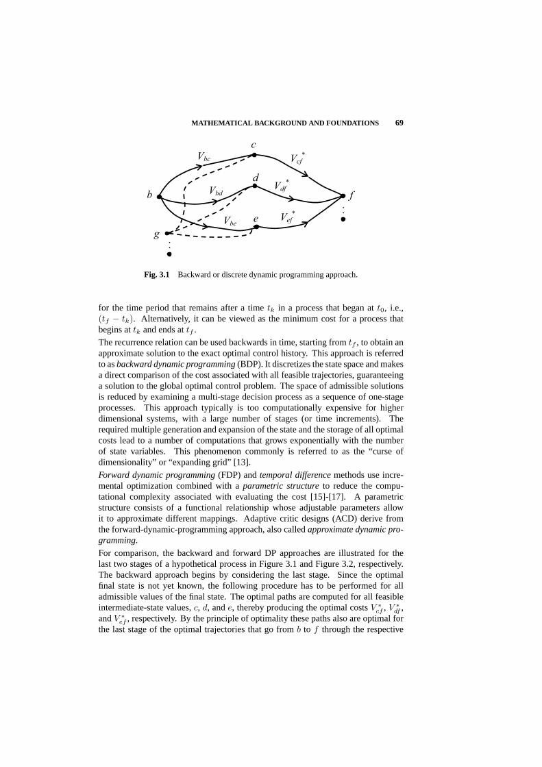
MATHEMATICAL BACKGROUND AND FOUNDATIONS 69
g
b
c
.
.Vef
*
Vdf*
Vcf*
Vbe
Vbd
Vbc
e
d
.
.
f
Fig. 3.1 Backward or discrete dynamic programming approach.
for the time period that remains after a timetk in a process that began att0, i.e.,(tf − tk). Alternatively, it can be viewed as the minimum cost for a process thatbegins attk and ends attf .
The recurrence relation can be used backwards in time, starting fromtf , to obtain anapproximate solution to the exact optimal control history. This approach is referredto asbackward dynamic programming(BDP). It discretizes the state space and makesa direct comparison of the cost associated with all feasible trajectories, guaranteeinga solution to the global optimal control problem. The space of admissible solutionsis reduced by examining a multi-stage decision process as a sequence of one-stageprocesses. This approach typically is too computationally expensive for higherdimensional systems, with a large number of stages (or time increments). Therequired multiple generation and expansion of the state and the storage of all optimalcosts lead to a number of computations that grows exponentially with the numberof state variables. This phenomenon commonly is referred to as the “curse ofdimensionality” or “expanding grid” [13].
Forward dynamic programming(FDP) andtemporal differencemethods use incre-mental optimization combined with aparametric structureto reduce the compu-tational complexity associated with evaluating the cost [15]-[17]. A parametricstructure consists of a functional relationship whose adjustable parameters allowit to approximate different mappings. Adaptive critic designs (ACD) derive fromthe forward-dynamic-programming approach, also calledapproximate dynamic pro-gramming.
For comparison, the backward and forward DP approaches are illustrated for thelast two stages of a hypothetical process in Figure 3.1 and Figure 3.2, respectively.The backward approach begins by considering the last stage. Since the optimalfinal state is not yet known, the following procedure has to be performed for alladmissible values of the final state. The optimal paths are computed for all feasibleintermediate-state values,c, d, ande, thereby producing the optimal costsV ∗
cf , V ∗df ,
andV ∗ef , respectively. By the principle of optimality these paths also are optimal for
the last stage of the optimal trajectories that go fromb to f through the respective

70 MODEL-BASED ADAPTIVE CRITIC DESIGNS
state values, e. g.,V ∗b(c)f = Vbc + V ∗
cf . Thus, if the last-stage’s costs,V ∗cf , V ∗
df , andV ∗
ef , are stored, then the total costsV ∗b(c)f , V ∗
b(d)f , andV ∗b(e)f can be compared to
find the optimal path fromb to f . For a process with more than two stages, the stateb would be unknown. Hence, the same computation would be carried out for allpossible state values, such asg in Figure 3.1, in order to determineV ∗
bf , V ∗gf , and
so on. The algorithm terminates when the initial stage is reached, where the state isknown from the initial conditions.
Unlike backward DP, forward DP algorithms progress forward in time, and theyapproximate the optimal control and future cost by considering only the current valueof the state. Supposea is the initial state of a two-stage process or, equivalently, thestate of an on-going process at the second-to-last stage, as outlined in Figure 3.2.Then,a is known and the costVab can be computed from the Lagrangian for a chosencontrol policy. The optimal cost over all future stages,V ∗
bf , is predicted by a function
approximator or parametric structure. Hence, the sum(Vab + V ∗bf ) can be minimized
with respect to the present value of the control, according to the recurrence relationof dynamic programming (Eq. 3.9). At the next stageb-c this procedure is repeated.The cost approximation, denoted byV , has been improved based on the informationgathered during the first stage. Therefore, the next path, fromc to f , is closer to theoptimal trajectory.
Adaptive critic designs reproduce the most general solution of FDP by derivingrecurrence relations for the optimal policy, the cost, and, possibly, their derivatives.The goal is to overcome the curse of dimensionality, while ensuring convergenceto a near-optimal solution over time. The following section introduces the basicadaptive-critic algorithm and the related proof of convergence.
3.2.2 The Adaptive Critic Algorithm
Adaptive critic designs are based on an algorithm that cycles between apolicy-improvement routineand avalue-determination operation. At each optimizing cycle,indexed by , the algorithm approximates the optimal control law (Eq. 3.3) and valuefunction (Eq. 3.8) based on the statexk. We distinguish between iteration overk, which represents the passage of time in the dynamic process, and over`, whichrelates to the search for an optimal solution. In off-line optimization, an ensemble ofstate vectors including all possible values ofxk is used during every cycle. In this
b cVbcVab Vcfa
*~
bfV *~
cfV
f
Fig. 3.2 Forward or approximate dynamic programming approach.
MATHEMATICAL BACKGROUND AND FOUNDATIONS 71
case, the entire process can be simulated fromt0 to tf . In on-line optimization, onecycle is carried out at each time step based on a single value ofxk, i. e., the actualstate, such thatk = `.
For simplicity, the following discussion is limited to the infinite-horizon optimalcontrol problem, where the final timetf tends to infinity. In this case, the costfunction to be minimized takes the form,
J = limtf→∞
tf−1∑tk=t0
L[x(tk),u(tk)] (3.10)
and the terminal cost can be set equal to zero [1].
The projected costV (xk+1, c) that a sub-optimal control lawc would incur fromtkto tf can be estimated from Eq. 3.7. Using the projected cost as a basis, the control-law and value-function approximations can be improved during every optimizationcycle,`. Over several cycles, the policy-improvement routine generates a sequenceof sub-optimal control lawsc` | ` = 0, 1, 2, . . .; the value-determination operationproduces a sequence of sub-optimal value functionsV` | ` = 0, 1, 2, . . .. Thealgorithm terminates whenc` and V` have converged to the optimal control lawand value function, respectively. The proof of convergence [5] is outlined in theAppendix.
Policy-Improvement Routine Given a value functionV (·, c`) corresponding to acontrol lawc`, animprovedcontrol law,c`+1, can be obtained as follows,
c`+1(xk) = arg minuk
L(xk,uk) + V (xk+1, c`) (3.11)
such thatV (xk, c`+1) ≤ V (xk, c`), for any value ofxk. Furthermore, the sequenceof functionsc` | ` = 0, 1, 2, . . . converges to the optimal control law,c∗(x).
Value-Determination Operation Given a control lawc, the value function can beupdated according to the following rule,
V`+1(xk, c) = L(xk,uk) + V`(xk+1, c) (3.12)
such that the sequenceV` | ` = 0, 1, 2, . . ., in concert with the policy-improvementupdate, converges to the optimal value functionV ∗(x).
The adaptive critic algorithm successively iterates between these two updates, asillustrated in Figure 3.3. The algorithm can begin in either box. The speed ofconvergence is dependent on the suitability of the initialized control law and valuefunction c0 and V0, as well as on the details of the adjustment rules. A simpleexample is given in Section 3.3.5. More detailed examples are given in [11, 18].
In the `th cycle,c`+1 is determined by the policy-improvement routine and can beused as the control lawc in the value-determination operation. Then, in the(`+1)th
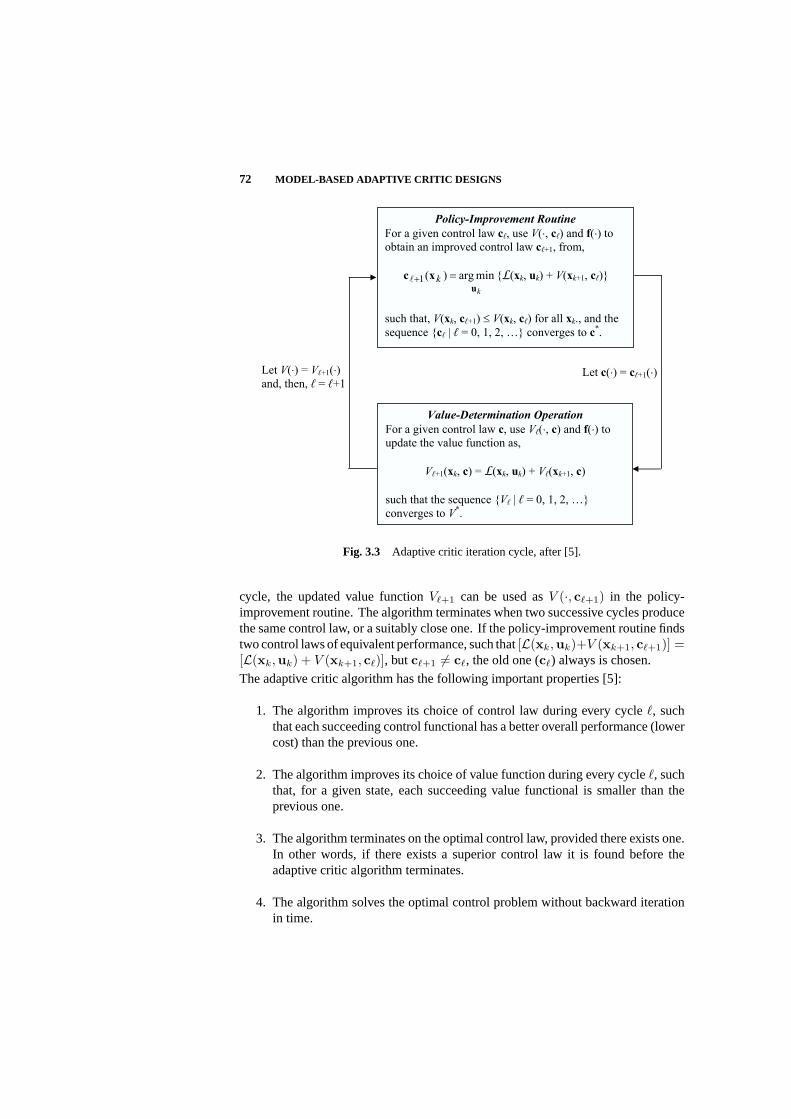
72 MODEL-BASED ADAPTIVE CRITIC DESIGNS
Policy-Improvement Routine
For a given control law c , use V( , c ) and f( ) to
obtain an improved control law c +1, from,
k
k
u
xc minarg)(1 L(xk, uk) + V(xk+1, c )
such that, V(xk, c +1) V(xk, c ) for all xk., and the
sequence c | = 0, 1, 2, converges to c*.
Let V( ) = V +1( )
and, then, = +1
Value-Determination Operation
For a given control law c, use V ( , c) and f( ) to
update the value function as,
V +1(xk, c) = L(xk, uk) + V (xk+1, c)
such that the sequence V | = 0, 1, 2,
converges to V*.
Let c( ) = c +1( )
Fig. 3.3 Adaptive critic iteration cycle, after [5].
cycle, the updated value functionV`+1 can be used asV (·, c`+1) in the policy-improvement routine. The algorithm terminates when two successive cycles producethe same control law, or a suitably close one. If the policy-improvement routine findstwo control laws of equivalent performance, such that[L(xk,uk)+V (xk+1, c`+1)] =[L(xk,uk) + V (xk+1, c`)], butc`+1 6= c`, the old one (c`) always is chosen.
The adaptive critic algorithm has the following important properties [5]:
1. The algorithm improves its choice of control law during every cycle`, suchthat each succeeding control functional has a better overall performance (lowercost) than the previous one.
2. The algorithm improves its choice of value function during every cycle`, suchthat, for a given state, each succeeding value functional is smaller than theprevious one.
3. The algorithm terminates on the optimal control law, provided there exists one.In other words, if there exists a superior control law it is found before theadaptive critic algorithm terminates.
4. The algorithm solves the optimal control problem without backward iterationin time.

ADAPTIVE CRITIC DESIGN AND IMPLEMENTATION 73
Properties 1 through 4 are demonstrated in the Appendix. Property 4 is fundamentalto the solution approach. The following section discusses on-line implementationsof the adaptive critic algorithm.
3.3 ADAPTIVE CRITIC DESIGN AND IMPLEMENTATION
The adaptive critic algorithm can be used to determine the optimal control law for adynamic process on or off line. In the latter case, control design is based on the modelof the system to be controlled, and the required values of the state are produced bysimulation. The adaptive critic cycle generates a control lawc` and a value functionV` for an ensemble of state values. The procedure is repeated for` = 0, 1, 2, . . ., untilthe algorithm terminates producingc∗ andV ∗. Subsequently,c∗ can be implementedto operate the system in Eq. 3.2 in an optimal fashion.
The adaptive critic algorithm also can be used on line. Unlike the Euler-Lagrangeequations and backward DP, the computation required by each iteration depends onlyon the present state,xk, and does not involve the final conditions (e. g.,λ(tf )).In on-line implementations state-vector values become available progressively intime asxk | k = 0, 1, 2, . . .. Then, the indices and k in Figure 3.3 coincideat every algorithmic cycle and moment in time. Although this procedure can beadopted for systems whose dynamic equation (Eq. 3.2) is known precisely, it isparticularly valuable when the system dynamics are not fully known or subject tochange. Then, the adaptive critic algorithm can be implemented on line, while thesystem is operating.
In on-line implementations, the control lawc`, generated by theth algorithmic cycle,is applied at timetk. Assuming that the plant is fully observable, theactualvalue ofthe present state,xk, is determined from available output measurements. The nextvalue of the state,xk+1, ispredictedthrough the model in Eq. 3.2. Hence, the controllaw and value function can be improved at every moment in timetk based on theobserved value ofxk. The optimal control law can be determined on line for systemswhose true dynamic characteristics are revealed only during actual operation. Sincethe adaptive critic algorithm improves upon any sub-optimal control law (sayc`−1), itusually is convenient to implementc` as soon as it is generated. The system convergesto optimal performance provided its dynamics remain unchanged. Otherwise, thealgorithm continues to improve the control and value functions incrementally, subjectto the varying dynamics. An underlying assumption is that the dynamic variationsoccur on a sufficiently large time scale with respect to the algorithmic cycles.
3.3.1 Overview of Adaptive Critic Designs
Adaptive critic designs implement approximate dynamic programming through recur-rence relations for the control law, the value function, and, possibly, their derivatives.The basic architectures can be classified in four categories [19, 20]:
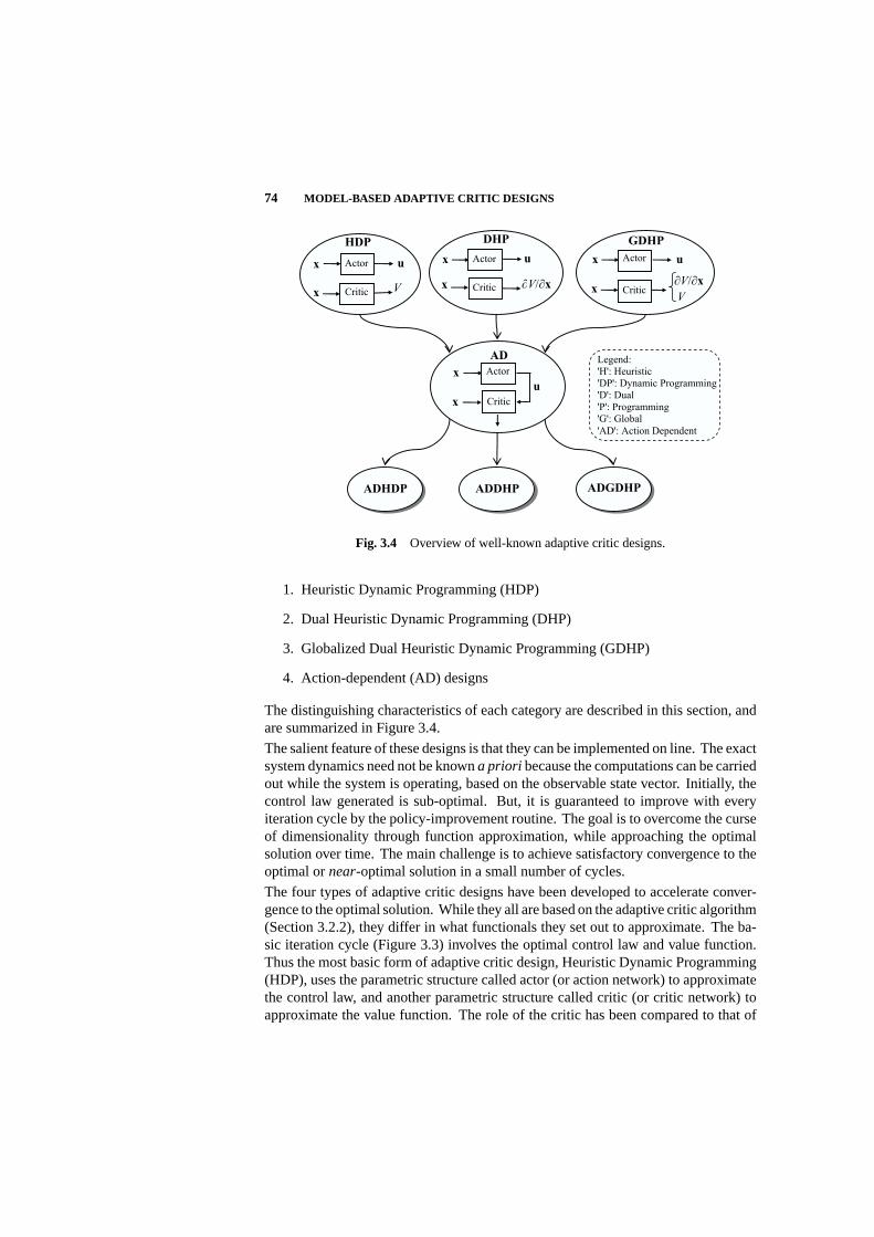
74 MODEL-BASED ADAPTIVE CRITIC DESIGNS
x
x
GDHP
u
CriticV/ x
V
Actor
x
x
DHP
V/ x
u
Critic
Actor
HDP
xV
ux
Critic
Actor
Legend:
'H': Heuristic
'DP': Dynamic Programming
'D': Dual
'P': Programming
'G': Global
'AD': Action Dependent
x
u
x
Critic
AD
Actor
ADHDP ADDHP ADGDHP
Fig. 3.4 Overview of well-known adaptive critic designs.
1. Heuristic Dynamic Programming (HDP)
2. Dual Heuristic Dynamic Programming (DHP)
3. Globalized Dual Heuristic Dynamic Programming (GDHP)
4. Action-dependent (AD) designs
The distinguishing characteristics of each category are described in this section, andare summarized in Figure 3.4.
The salient feature of these designs is that they can be implemented on line. The exactsystem dynamics need not be knowna priori because the computations can be carriedout while the system is operating, based on the observable state vector. Initially, thecontrol law generated is sub-optimal. But, it is guaranteed to improve with everyiteration cycle by the policy-improvement routine. The goal is to overcome the curseof dimensionality through function approximation, while approaching the optimalsolution over time. The main challenge is to achieve satisfactory convergence to theoptimal ornear-optimal solution in a small number of cycles.
The four types of adaptive critic designs have been developed to accelerate conver-gence to the optimal solution. While they all are based on the adaptive critic algorithm(Section 3.2.2), they differ in what functionals they set out to approximate. The ba-sic iteration cycle (Figure 3.3) involves the optimal control law and value function.Thus the most basic form of adaptive critic design, Heuristic Dynamic Programming(HDP), uses the parametric structure called actor (or action network) to approximatethe control law, and another parametric structure called critic (or critic network) toapproximate the value function. The role of the critic has been compared to that of

ADAPTIVE CRITIC DESIGN AND IMPLEMENTATION 75
“reinforcement” in psychology, and to the “utility function” in utility theory [21].The critic provides the actor with a performance measure for its present actions byanticipating and evaluating future events. In practice, HDP converges slowly becausethe parameters of this architecture ultimately are updated based on a scalar evaluationfunction, i. e.,V .
An alternative approach referred to as Dual Heuristic Programming (DHP) was firstproposed in [21, 22]. DHP uses the critic to approximate the derivatives of thevalue function with respect to the state, i. e.,∂V/∂xk. It correlates the parametersof the architecture to a larger number of dependent variables. The actor is used toapproximate the control law, as in all other adaptive critic designs. An algorithmfor updating the DHP functionals can be obtained from the policy-improvementroutine and the value-determination operation, as explained in Section 3.3.3. Inapplications [23, 24], the DHP algorithm has been shown to find the optimal solutionmore rapidly (with less iteration cycles) than HDP. However, due to the use ofderivative information, the relationships for updating the control and value-derivativefunctionals are more involved. Furthermore, since the DHP critic approximates avector functional, the problem of function approximation is more challenging.
Many other methodologies have been proposed to alleviate some of the difficultiesmentioned above. For example, Globalized Dual Heuristic Programming (GDHP)combines the advantages of both the HDP and DHP architectures [16, 25, 26]. InGDHP the critic approximates both the value function and its derivatives. Action-dependent (AD) versions of these approaches use a parametric structure, again re-ferred to as critic, to approximate a value function that dependsexplicitly on thecontrol (as shown in Figure 3.4). The motivation behind this [27] and other method-ologies (e. g., [28]) is to achieve faster convergence to the optimal solution and tosimplify the problem of function approximation.
In summary, an adaptive critic architecture consists of a parametric structure, thecritic, that approximates the value function (Eq. 3.4) or a closely-related quantity,and another parametric structure, the actor, that approximates the control law. Oncethe functions to be approximated are chosen, an algorithm that updates them atevery cycle can be obtained from the policy-improvement routine and the value-determination operation in Section 3.2.2. The objective is to produce two sequencesof functions that eventually converge to the optimal solution.
3.3.2 Function Approximation
Three functionals play a key role in all adaptive critic designs. They are:
• The control law
• The value function
• The model of the system to be controlled
The objective of the adaptive critic algorithm is to progressively improve its approx-imation of the optimal control lawc∗(xk) and value functionV ∗(xk). A model of

76 MODEL-BASED ADAPTIVE CRITIC DESIGNS
the system (such as Eq. 3.2) is required in order to predict the next value of the statexk+1 at every iteration cycle (Figure 3.3). Hence, designs based on this algorithmoften are referred to asmodel-based adaptive critics. When the system’s behavior ispartly unanticipated the model provides an approximation to its dynamics [19].
The sequences of functions generated by the adaptive critic algorithm are synthe-sized by a convenient parametrization or function approximator that captures therelationship between the dependent and independent variables. Without the use ofan appropriate parametric structure each function, sayuk = c`(xk), would need tobe represented by a lookup table. For large state and control spaces it is infeasibleto carry out the required computation (eq.s 3.11 and 3.12) with lookup-table rep-resentations ofc`, V`, c`+1, andV`+1. Moreover, it usually is desirable to obtaina functional representation of the optimal control and value functions once the al-gorithm converges. Therefore, a parametric structure that, ultimately, is capable ofapproximating the optimal solution must be chosen.
A suitable function approximatoror parametric structure has the following charac-teristics:
• It is differentiable;
• It approximates the desired function with less complexity than a lookup-tablerepresentation;
• It is supplied with apposite algorithms for computing the parameter values;
• It is capable of approximating the optimal shape of the function within thedesired accuracy.
There are many theoretical and practical issues associated with the problem of func-tion approximation. The most important ones pertain to the effect that functionapproximation has on convergence. In order for the original proof (in the Appendix)to hold, this process must be consistent with the policy-improvement routine andvalue-determination operation in Section 3.2.2. Additional details can be found in[29]-[31].
We assume that the actor is a suitable parametric structurec(xk,a), wherea is a vectorof parameters to be optimized by the policy-improvement routine. The functionapproximator’s parameters are updated at every cycle,`, such thatc(xk,a`) ≈c`(xk). Then, the computational complexity of the adaptive critic algorithm isreduced at every cycle. Upon termination of the algorithm (whenc` → c∗), theoptimal control is readily approximated asc(xk,a∗) ≈ c∗(xk).The parameters of the function approximator must be determined at every cycle of thealgorithm without compromising convergence. This process, in itself, may requireone or more iterations. The following sections describe how function approximationcan be combined with the policy-improvement routine and the value-determinationoperation (Section 3.2.2) to produce heuristic and dual-heuristic adaptive critic de-signs.

ADAPTIVE CRITIC DESIGN AND IMPLEMENTATION 77
3.3.3 Derivation of the Heuristic and Dual-Heuristic Dynamic ProgrammingAlgorithms
In on-line implementations of adaptive critic designs the control and value functionapproximations are updated incrementally over time. With one available value ofthe state,xk, the minimization problem in Eq. 3.11 can be solved by computing thestationary point of the scalar functionV (xk, c`) ≡ [L(xk,uk)+V (xk+1, c`)]. Thispoint is defined as the value ofuk that satisfies theoptimality condition,
∂V (xk, c`)∂uk
=∂L(xk,uk)
∂uk+
[∂f(xk,uk)
∂uk
]T∂V (xk+1, c`)
∂xk+1= 0 (3.13)
along with the followingconvexity condition:
∂2V (xk, c`)∂u2
k
> 0 (3.14)
This condition requires a positive definite Hessian matrix [32]. The gradient of ascalar function [32], e. g.,∂V/∂xk, is defined as a column vector. The stationarycontrol value can be used to improve upon the control law approximationc` at themoment in timetk. Rules for updating the critic on line are similarly derived, asshown in the following sections.
Heuristic Dynamic Programming (HDP) Algorithm
In Heuristic Dynamic Programming, the actor is a parametric structurec with pa-rametersa that is used to approximate the control law. The critic is a parametricstructureV , with parametersw, that is used to approximate the value function, i. e.:
c(xk,a`) ≈ c`(xk) (3.15)
V (xk,w`) ≈ V`(xk, c) (3.16)
The value function estimate is assumed to be acomposite functionof xk, sinceuk = c(xk) and system dynamics are known (Eq. 3.2). The state is its sole input,as this is the action-independent version of HDP. The optimal value function alsois a function solely of the state, as shown in Eq. 3.8. When the chosen parametricstructures are differentiable, the optimality condition (Eq. 3.13) generates a sequenceof successively-improving control lawsc` | ` = 0, 1, 2, . . .. Concurrently, thevalue-determination operation (Eq. 3.12) generates a sequence of successively-improving value functionsV` | ` = 0, 1, 2, . . .. An HDP algorithm that iteratesbetween these two operations is shown below. At every cycle`, the actor parametersare updated based on the improved control lawc`+1, and the critic parameters areupdated based on the improved value functionV`+1.

78 MODEL-BASED ADAPTIVE CRITIC DESIGNS
Heuristic-Dynamic-Programming Actor Update Suppose a control-law approx-imator, c(·,a`), and a corresponding value-function approximator,V (·,w`), aregiven. Then, an improved control-law approximatorc(·,a`+1) can be obtained bycomputing a desired control vectoruD
k , such that,
∂V (xk,w`)∂uk
∣∣∣∣∣uk=uD
k
=
[∂L(xk,uk)
∂uk+
(∂f(xk,uk)
∂uk
)T∂V (xk+1,w`)
∂xk+1
]∣∣∣∣∣uk=uD
k
= 0
(3.17)and the matrix[∂2V (xk,w`)/∂u2
k]|uk=uDk
is positive definite.
The improved actor parameters,a`+1, can be computed as follows,
a`+1 = arg minauD
k − c(xk,a) (3.18)
where,uDk ≡ c`+1(xk), thereforec(xk,a`+1) ≈ c`+1(xk).
Heuristic-Dynamic-Programming Critic Update Given the improved control-lawapproximatorc(·,a`+1) and the value-function approximatorV (·,w`), an improvedvalue-function approximatorV (·,w`+1) can be obtained by computing its desiredvalue,
V Dk ≡ V`+1(xk, c) = L(xk,uk) + V (xk+1,w`) (3.19)
with uk = c(xk,a`+1), and, subsequently, by determining the improved criticparameters,
w`+1 = arg minwV D
k − V (xk,w) (3.20)
such that,V (xk,w`+1) ≈ V`+1(xk, c).
There exist other approaches for updating the actor based on the optimality condition.One possibility is to obtain the improved actor parameters by minimizing the right-hand side of Eq. 3.17 directly with respect toa:
a`+1 = arg mina
[∂L(xk,uk)
∂uk+
(∂f(xk,uk)
∂uk
)T∂V (xk+1,w`)
∂xk+1
]∣∣∣∣∣uk=c(xk,a)
(3.21)Although this method reduces the actor update to one step, it may be computationallyless efficient and less reliable.
Dual Heuristic Dynamic Programming (DHP) Algorithm
In Dual Heuristic Dynamic Programming, the critic approximates a sequence offunctionals,λ` | ` = 0, 1, 2, . . ., that ultimately converges to the derivative of the

ADAPTIVE CRITIC DESIGN AND IMPLEMENTATION 79
optimal value function with respect to the state, defined as:
λ∗(x∗k) ≡ ∂V ∗(x∗k)∂x∗k
(3.22)
In essence, the role of the critic is to generate the costate or adjoint vector in theHamilton-Jacobi-Bellman(HJB) equation, estimating the cost sensitivity to stateperturbations. In the HJB approach, the Hamiltonian (Eq. 3.5) is defined by adjoiningthe dynamic equation (Eq. 3.2) to the Lagrangian by∂V/∂xk.
A parametric structurec with parametersa, the actor, is used to approximate thecontrol law. Another parametric structureλ with parametersω, the critic, is used toapproximate the derivative of the value function with respect to the state:
c(xk,a`) ≈ c`(xk) (3.15)
λ(xk, ω`) ≈ ∂V`(xk, c)∂xk
≡ λ`(xk, c) (3.23)
When the chosen parametric structures are differentiable, the optimality condition(Eq. 3.13) can be used to generate a sequence of successively-improving controllawsc` | ` = 0, 1, 2, . . ..The value-determination operation (Eq. 3.12) is differentiated with respect to thestate to obtain a recurrence relation for the functionλ:
∂V`+1(xk, c)∂xk
≡ λ`+1(xk, c) =∂L(xk,uk)
∂xk+
[∂c(xk)∂xk
]T∂L(xk,uk)
∂uk
+[∂f(xk,uk)
∂xk
]T∂V`(xk+1, c)
∂xk+1
+[∂c(xk)∂xk
]T [∂f(xk,uk)
∂uk
]T∂V`(xk+1, c)
∂xk+1(3.24)
Equation 3.24 generates the sequence of successively-improving value functionderivativesλ` | ` = 0, 1, 2, . . ., as the control law sequence is generated. A DHPalgorithm that, at every step, updates the actor parameters based on the improvedcontrol law,c`+1, and updates the critic parameters based on the improved value-function derivative,λ`+1, is given below.
Dual-Heuristic-Programming Actor Update Suppose a control-law approxima-tor c(·,a`) and a corresponding value-function-derivative approximatorλ(·, ω`) aregiven. Then, an improved control-law approximatorc(·,a`+1) can be obtained by
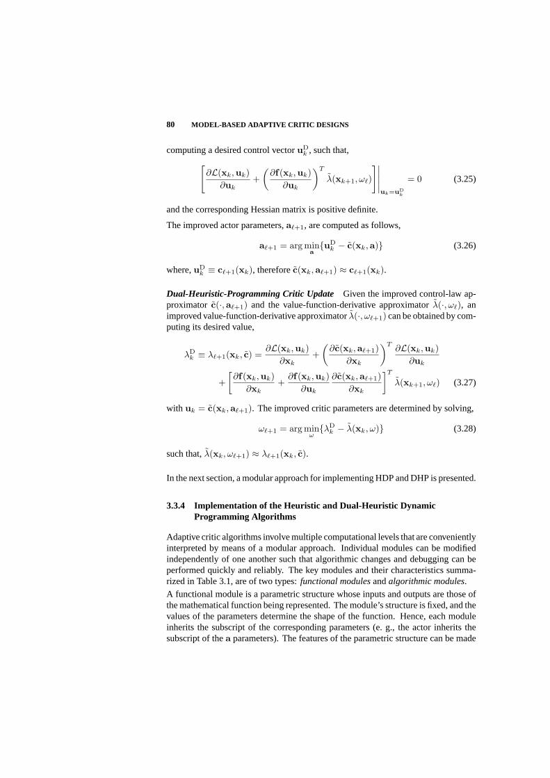
80 MODEL-BASED ADAPTIVE CRITIC DESIGNS
computing a desired control vectoruDk , such that,
[∂L(xk,uk)
∂uk+
(∂f(xk,uk)
∂uk
)T
λ(xk+1, ω`)
]∣∣∣∣∣uk=uD
k
= 0 (3.25)
and the corresponding Hessian matrix is positive definite.
The improved actor parameters,a`+1, are computed as follows,
a`+1 = arg minauD
k − c(xk,a) (3.26)
where,uDk ≡ c`+1(xk), thereforec(xk,a`+1) ≈ c`+1(xk).
Dual-Heuristic-Programming Critic Update Given the improved control-law ap-proximator c(·,a`+1) and the value-function-derivative approximatorλ(·, ω`), animproved value-function-derivative approximatorλ(·, ω`+1) can be obtained by com-puting its desired value,
λDk ≡ λ`+1(xk, c) =
∂L(xk,uk)∂xk
+(
∂c(xk,a`+1)∂xk
)T∂L(xk,uk)
∂uk
+[∂f(xk,uk)
∂xk+
∂f(xk,uk)∂uk
∂c(xk,a`+1)∂xk
]T
λ(xk+1, ω`) (3.27)
with uk = c(xk,a`+1). The improved critic parameters are determined by solving,
ω`+1 = arg minωλD
k − λ(xk, ω) (3.28)
such that,λ(xk, ω`+1) ≈ λ`+1(xk, c).
In the next section, a modular approach for implementing HDP and DHP is presented.
3.3.4 Implementation of the Heuristic and Dual-Heuristic DynamicProgramming Algorithms
Adaptive critic algorithms involve multiple computational levels that are convenientlyinterpreted by means of a modular approach. Individual modules can be modifiedindependently of one another such that algorithmic changes and debugging can beperformed quickly and reliably. The key modules and their characteristics summa-rized in Table 3.1, are of two types:functional modulesandalgorithmic modules.
A functional module is a parametric structure whose inputs and outputs are those ofthe mathematical function being represented. The module’s structure is fixed, and thevalues of the parameters determine the shape of the function. Hence, each moduleinherits the subscript of the corresponding parameters (e. g., the actor inherits thesubscript of thea parameters). The features of the parametric structure can be made

ADAPTIVE CRITIC DESIGN AND IMPLEMENTATION 81
Module:Implementation
of:Inputs: Outputs: Architecture:
),(~ ac xk c ( ) Both
),(~
wV xk V ( ) HDP
),(~
xk ( ) DHP
Function
approximatione, p, and g~ ( , ) g~ ( , +1) Both
xk, ),(~ ac ,
and ),(~
wV
Dku HDPPolicy-
improvement
routine xk, ),(~ ac ,
and ),(~
Dku DHP
xk, ),(~1ac ,
and ),(~
wV
DkV HDPValue-
determination
operation xk, ),(~1ac ,
and ),(~
Dk
DHP
Actor
Critic
Parameter
update
Actor
target
Critic
target
Table 3.1 Functional and algorithmic modules and their characteristics within HeuristicDynamic Programming (HDP) and Dual Heuristic Programming (DHP) architectures.
accessible to and modified by other modules. In most programming languages thisis easily achieved, for example by making these featuresglobal variables[33]. Theactor and the critic constitute the key functional modules.
An algorithmic module may involve one or more iterations whose purpose is toupdate parameters, solve the optimality condition, and compute the value function orits derivatives. The details of each module depend on the adaptive critic design andparametric structures. Table 3.1 shows how the properties of each module depend onthe chosen architecture. Using this notation, both the HDP and DHP algorithms canbe described by the diagram in Figure 3.5. The solid lines illustrate the flow of inputand output information between the modules. The dashed lines in Figure 3.5 indicatethat the updated functional modules replace the preceding ones. The modules’ inputsand outputs are listed in Table 3.1.
3.3.4.1 Parameter-Update Module for Function ApproximationThe actor andthe critic functional modules represent the corresponding parametric structures, asillustrated in Table 3.1. These structures may consist of neural networks, polynomials,splines [34], or any other differentiable mappings with adjustable parameters. Thevalues of the parameters are adjusted by the parameter-update module during every

82 MODEL-BASED ADAPTIVE CRITIC DESIGNS
Actor Critic
Actor +1
Critic +1
Parameter
update
Actor
target
Critic
target
Parameter
update
Fig. 3.5 Modular description of the′th iteration cycle in the HDP and DHP algorithms.
cycle, `, of the adaptive critic algorithm. For example, in the case of a neuralnetwork this module represents a training algorithm such as backpropagation [35].In temporal-difference methods it represents the learning algorithm for updating theweight vector of the chosen basis functions.
In general, the functions in a sequenceg`(p) | ` = 0, 1, 2, . . . must be succes-sively approximated by a parametric structure,g(p, υ), with inputp and adjustableparametersυ. The functions may comprise control laws or value-related functions,depending on which functional module is being updated. Eventually, the sequenceconverges to the optimal functiong∗(p) ≈ g(p, υ). Prior to this,g`+1(p) representsan estimate ofg∗(p) that has been improved with respect to the preceding functiong`(p) during the iteration cycle.
The parameter-update module determines the value of the parametersυ`+1 for whichg(p, υ`+1) most closely approximatesg`+1(p). The parameters are initialized witheither random variables or prior values. In subsequent cycles, an estimate of theparameters already is available inυ`. This estimate can be improved by minimizinga specified error, denoted in general bye, with respect to the parameter values. Theimproved parameter values,υ`+1, replaceυ` in the updated structureg(p, υ`+1) (asillustrated in Figure 3.6). Every error-minimization process may involve one or more
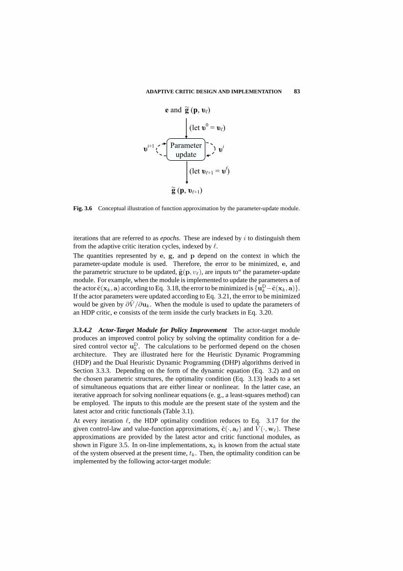
ADAPTIVE CRITIC DESIGN AND IMPLEMENTATION 83
e and g~ (p, )
(let0 = )
i+1 Parameter
updatei
g~ (p, +1)
(let +1 = f)
Fig. 3.6 Conceptual illustration of function approximation by the parameter-update module.
iterations that are referred to asepochs. These are indexed byi to distinguish themfrom the adaptive critic iteration cycles, indexed by`.
The quantities represented bye, g, and p depend on the context in which theparameter-update module is used. Therefore, the error to be minimized,e, andthe parametric structure to be updated,g(p, υ`), are inputs to“ the parameter-updatemodule. For example, when the module is implemented to update the parametersa ofthe actorc(xk,a) according to Eq. 3.18, the error to be minimized isuD
k −c(xk,a).If the actor parameters were updated according to Eq. 3.21, the error to be minimizedwould be given by∂V /∂uk. When the module is used to update the parameters ofan HDP critic,e consists of the term inside the curly brackets in Eq. 3.20.
3.3.4.2 Actor-Target Module for Policy ImprovementThe actor-target moduleproduces an improved control policy by solving the optimality condition for a de-sired control vectoruD
k . The calculations to be performed depend on the chosenarchitecture. They are illustrated here for the Heuristic Dynamic Programming(HDP) and the Dual Heuristic Dynamic Programming (DHP) algorithms derived inSection 3.3.3. Depending on the form of the dynamic equation (Eq. 3.2) and onthe chosen parametric structures, the optimality condition (Eq. 3.13) leads to a setof simultaneous equations that are either linear or nonlinear. In the latter case, aniterative approach for solving nonlinear equations (e. g., a least-squares method) canbe employed. The inputs to this module are the present state of the system and thelatest actor and critic functionals (Table 3.1).
At every iteration`, the HDP optimality condition reduces to Eq. 3.17 for thegiven control-law and value-function approximations,c(·,a`) andV (·,w`). Theseapproximations are provided by the latest actor and critic functional modules, asshown in Figure 3.5. In on-line implementations,xk is known from the actual stateof the system observed at the present time,tk. Then, the optimality condition can beimplemented by the following actor-target module:
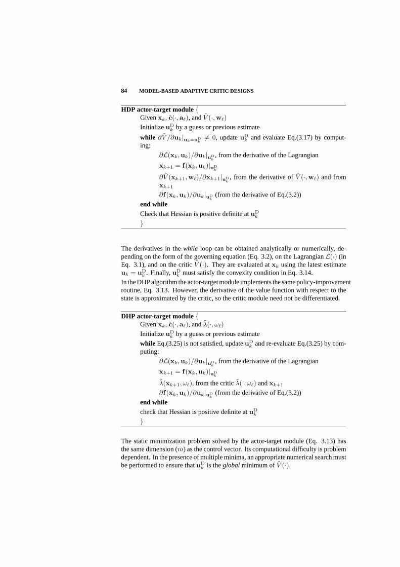
84 MODEL-BASED ADAPTIVE CRITIC DESIGNS
HDP actor-target moduleGivenxk, c(·,a`), andV (·,w`)Initialize uD
k by a guess or previous estimate
while ∂V /∂uk|uk=uDk6= 0, updateuD
k and evaluate Eq.(3.17) by comput-ing:
∂L(xk,uk)/∂uk|uDk
, from the derivative of the Lagrangian
xk+1 = f(xk,uk)|uDk
∂V (xk+1,w`)/∂xk+1|uDk
, from the derivative ofV (·,w`) and fromxk+1
∂f(xk,uk)/∂uk|uDk
(from the derivative of Eq.(3.2))
end whileCheck that Hessian is positive definite atuD
k
The derivatives in thewhile loop can be obtained analytically or numerically, de-pending on the form of the governing equation (Eq. 3.2), on the LagrangianL(·) (inEq. 3.1), and on the criticV (·). They are evaluated atxk using the latest estimateuk = uD
k . Finally,uDk must satisfy the convexity condition in Eq. 3.14.
In the DHP algorithm the actor-target module implements the same policy-improvementroutine, Eq. 3.13. However, the derivative of the value function with respect to thestate is approximated by the critic, so the critic module need not be differentiated.
DHP actor-target moduleGivenxk, c(·,a`), andλ(·, ω`)Initialize uD
k by a guess or previous estimate
while Eq.(3.25) is not satisfied, updateuDk and re-evaluate Eq.(3.25) by com-
puting:
∂L(xk,uk)/∂uk|uDk
, from the derivative of the Lagrangian
xk+1 = f(xk,uk)|uDk
λ(xk+1, ω`), from the criticλ(·, ω`) andxk+1
∂f(xk,uk)/∂uk|uDk
(from the derivative of Eq.(3.2))
end whilecheck that Hessian is positive definite atuD
k
The static minimization problem solved by the actor-target module (Eq. 3.13) hasthe same dimension (m) as the control vector. Its computational difficulty is problemdependent. In the presence of multiple minima, an appropriate numerical search mustbe performed to ensure thatuD
k is theglobalminimum ofV (·).

ADAPTIVE CRITIC DESIGN AND IMPLEMENTATION 85
3.3.4.3 Critic-Target Module for Value Determination The critic-target modulecomputes an improved value function or value-function derivative for the presentstate,xk, according to the value-determination operation. The value of the improvedfunction, denoted by the superscript(·)D, can be used to update the critic parametersby means of the parameter-update module. Since the input/output characteristics ofthe critic depend on the chosen architecture, so do the computations performed bythe critic-target module. In this section, the critic-target module is illustrated for theHDP and DHP algorithms derived in Section 3.3.3.
In the HDP algorithm, a critic-update routine is obtained by combining the originalvalue-determination operation (Eq. 3.12) with function approximation. The critic-target module computes the improved valueV D
k based onxk and on the latest actorand critic approximations,c(·,a`+1) andV (·,w`).
HDP critic-target module Givenxk, c(·,a`+1), andV (·,w`)EvaluateV D
k from Eq.(3.19) by computing:
L(xk,uk), usinguk = c(xk,a`+1)xk+1 = f(xk,uk), usinguk = c(xk,a`+1)V (xk+1,w`), from the criticV (·,w`) andxk+1
The above algorithm implies that the actor parameters already have been updatedfrom a` to a`+1 according to the HDP actor update (Section 3.3.3).
Similarly, in DHP the critic-target module computes the desired value-functionderivative,λD
k , according to the critic-update operation. As before,λDk is com-
puted from the present state of the system,xk, and from the latest actor and criticstructures,c(·,a`+1) andλ(·, ω`). Then, the critic parameters can be updated fromω` to ω`+1 by the parameter-update module. The DHP critic-target module imple-ments a recurrence relation (Eq. 3.27) that is obtained by differentiating the originalvalue-determination operation (Eq. 3.12).
The derivatives in the critic-target module can be obtained analytically or numerically,depending on the form of the governing equation (Eq. 3.2), on the LagrangianL(·) (inEq. 3.1), and on the actorc(·). All of these quantities are evaluated at the present statexk and at the control value produced by the updated actor, i. e.,uk = c(xk,a`+1).
3.3.5 Example: Linear Quadratic Problem
Linear-quadratic (LQ) problems [1] involve a linear dynamic equation and a quadraticcost function. For this class of optimal control problems the solution can be computedby means of amatrix Riccati Equation[1]. Their solution by an adaptive criticapproach is demonstrated to illustrate the concepts introduced in the previous sections.

86 MODEL-BASED ADAPTIVE CRITIC DESIGNS
DHP critic-target module Givenxk, c(·,a`+1), andλ(·, ω`)EvaluateλD
k from Eq.(3.27) by computing:
∂L(xk,uk)/∂uk and ∂L(xk,uk)/∂xk, from the derivatives of theLagrangian
Usinguk = c(xk,a`+1)∂f(xk,uk)/∂uk and ∂f(xk,uk)/∂xk (from the derivatives ofEq.(3.2)),
Usinguk = c(xk,a`+1)xk+1 = f(xk,uk), usinguk = c(xk,a`+1)λ(xk+1, ω`), from the criticλ(·, ω`) andxk+1
∂c(xk,a`+1)/∂xk, from the derivative of the actorc(·,a`+1)
A quadratic cost function of the form,
J = limtf→∞
12
tf−1∑tk=t0
[xTk Qxk + uT
k Ruk] (3.29)
is to be minimized subject to thelinear time-invariant(LTI) dynamic equation
xk+1 = Fxk + Guk (3.30)
By assuming that the optimal value function is quadratic,
V ∗(x∗k) =12x∗k
T Px∗k (3.31)
it can be proven [13] that the LQ optimal control law has the form,
u∗k = −C(x∗k − xR) (3.32)
where,xR represents the reference state value. The problem’s objective is to deter-mine the matricesC andP that bring the state to the valuexR, while optimizing Eq.3.29 subject to Eq. 3.30.
Typically, the gain matrixC is obtained from the Riccati matrixP after solving aRiccati equation [1]. Here, we determine the optimal control and value functionusing the DHP approach. The functions to be calculated are the control law,c, andthe value function derivative,λ. From eq.s 3.31 and 3.32, it can be deduced thatpolynomials constitute suitable approximating structures for these functions. Byconsidering the elements ofC as the actor parameters (a) and the elements ofP as

ADAPTIVE CRITIC DESIGN AND IMPLEMENTATION 87
the critic parameters (ω), the DHP actor and critic are given by,
c(xk,a`) = −C`(xk − xR) (3.33)
λ(xk, ω`) = P`xk (3.34)
Q, R, andP` are symmetric, positive-definite matrices. The DHP actor and criticupdates (Section 3.3.3) are used to update the elements ofC` andP` at every cycle,`, of the adaptive critic algorithm.
The LQ problem can be solved on line by using the observed value of the statexk
during the`th cycle of the DHP algorithm (letting = k). After the actor and criticparameters are initialized toC0 andP0 the iterative process begins. Every cyclecomprises an actor update followed by a critic update. During the`th cycle the DHPactor update is carried out for the givenxk, c`, andλ`. The DHP actor-target module(Section 3.3.4.2) computesuD
k from Eq. 3.25, which takes the form
RuDk + GT P`(Fxk + GuD
k ) = 0 (3.35)
The new actor parametersC`+1 are determined by the parameter-update module(Section 3.3.4.1). According to Eq. 3.26, this can be achieved by minimizing theerroruD
k + C(xk − xR) with respect toC.
During the same cycle,, the DHP critic update is carried out for the givenxk, c`+1,andλ`. The DHP critic-target module (Section 3.3.4.3) computesλD
k from Eq. 3.27,which takes the form
λDk = Qxk + CT
`+1RC`+1xk + [F + GC`+1]T P`(F−GC`+1)xk (3.36)
The new critic parametersP`+1 are determined by the parameter-update module byminimizing the errorλD
k −Pxk with respect toP.
In this simple example the parameter-update module performs a linear minimizationto adjust the actor and the critic functionals (eq.s 3.33 and 3.34). In both cases, anerror with the formb − Ax is to be minimized with respect toA. Since thereare more unknowns (elements inA) than there are equations (error elements), theproblem is underdetermined. Hence, even in this simple case there exist multiplealternatives for the design of the parameter-update module (including least-squaresmethods). This usually is the most challenging aspect of the implementation and islikely to affect convergence greatly.
LQ problems are a class of control problems for which there exist more effectivemethods of solution than adaptive critic designs. This example is offered mainly forillustrative purposes. Nevertheless, if the actual system dynamics were to differ fromEq. 3.30 while retaining this linear form, the adaptive critic approach described herecould be implemented to perfect the control law (Eq. 3.33) on line. Thus, a similarmethod has been applied to aircraft optimal control in [40, 41].

88 MODEL-BASED ADAPTIVE CRITIC DESIGNS
3.4 DISCUSSION
This chapter focuses on on-line implementations of adaptive critic designs, where theactor and the critic are updated incrementally every time a state value is observed.Clearly, this approach is not always the most effective way to solve an optimal controlproblem. For example, when uncertainties and plant dynamics satisfy appropriateassumptions, other designs can be implemented more easily and effectively. Adaptivecritic designs present many challenges, including intricate implementation detailsand lack of performance guarantees. Nevertheless, they remain an important area ofresearch with many promises and accomplishments. Their most significant featureis that they can be used to develop control systems that canlearn to improve theirperformance over time subject to the actual plant dynamics.
Because the behavior of most plants cannot be fully anticipateda priori, adaptivecritic designs have been investigated for a wide range of applications. The DHPmethod has been successfully implemented to prevent cars from skidding whendriving over unexpected patches of ice [36]. DHP-based controllers have beendeveloped for missile interception [37] and for aircraft auto-landing [38]. Recently,adaptive critic designs have been used to replace the automatic voltage generatorand the turbine governor of a turbogenerator connected to the power grid [24]. Inthis research, DHP is shown to converge faster than HDP, especially in cases wherethe system’s dynamics and operating conditions change unexpectedly. Also, DHPhas been used to improve the performance of an aircraft controller on line in thepresence of unmodelled dynamics, control failures, and parameter variations [39].These numerical simulations show that learning can prevent loss of control duringcritical maneuvers while they are experienced by the controller for the first time.Another possible application of adaptive critic designs is on-line state estimation,which can be formulated as an optimal control problem (Section 3.2.1) where thecontrol,u, is replaced by the estimate of the state.
3.5 SUMMARY
This chapter provides an introduction to the field of model-reference adaptive criticdesigns. These methods seek optimality in the most general case. Their use for the on-line approximate solution of infinite-horizon optimal control problems is emphasizedhere. Section 3.2 presents basic background material, including Howard’s adaptivecritic algorithm or iteration cycle, which forms the basis of most ACD. The cyclecomprises a policy-improvement routine and a value-determination operation that canbe used in sequence to improve the approximate solution over time. By combining thisbasic iteration cycle with function approximation a variety of adaptive critic designscan be obtained, as described in Section 3.3. The Heuristic and Dual-HeuristicDynamic Programming (HDP and DHP) algorithms are derived in this section. Bothalgorithms can be implemented by a streamlined modular approach. This is based ontwo functional modules, the actor and the critic, and on three algorithmic modules,

SUMMARY 89
the parameter update, the actor target, and the critic target. Adaptive critic designshave been applied to a variety of problems, ranging from control of automobiles toregulation of turbogenerators. The DHP approach is demonstrated in Section 3.3.5for a simple linear-quadratic problem. A purpose of this chapter is to motivate thefurther exploration of ACD for the control and estimation of complex systems.
Appendix: Proof of Convergence for The Adaptive Critic AlgorithmThe following proof has been adapted from [5]. Given a generic control lawuk =c(xk), the following recurrence relation can be found by inspection from eq.s 3.4and 3.7
V (xk, c) = L(xk,uk) + V (xk+1, c) (3.37)
where, the value functionV is not necessarily optimal. For a process with a verylarge number of stages (or time increments), the total costJ in Eq. 3.1 can growwithout limit astf tends to infinity. Therefore, it is convenient to define anaveragetotal costcorresponding to the control lawc, that has the same optimality conditionsas Eq. 3.1
Jc = limtf→∞
1tf
tf−1∑tk=t0
L[x(tk),u(tk)] (3.38)
Also, astf approaches infinity in the limit, it is reasonable to let the terminal costϕ[x(tf )] equal zero [1]. Subsequently, arelative value functionthat has value inproving convergence of the adaptive critic algorithm can be defined as,
υc(xk) = limtf→∞
tf−1∑tk=t0
[L(xk, c)− Jc], x(t0) = x(tk) (3.39)
such that,Jc + υc(xk) = L(xk,uk) + V (xk+1, c) (3.40)
The relative value function differs from the original one by a constant that, under agiven policy, can be eliminated by considering the difference in relative values, e. g.,υc(xd)−υc(xe), representing the additional cost caused by starting at stated, ratherthan at statee.
Suppose that a control lawcA has been evaluated for the operation of the system, butthe adaptive critic algorithm has produced a control lawcB 6= cA. Then, property1 of the algorithm can be proven by showing that the new control law has a smalleraverage cost, i. e.,JB ≤ JA, or J∆ ≡ (JA − JB) ≥ 0. Since, Eq. 3.37 and 3.40can be written solely in terms ofxk anduk through Eq. 3.2, the subscriptk can beomitted and the equations written with respect tox, implying a generic moment intime. If the control lawcB was chosen overcA by the policy-improvement routine,then the following relationship applies,
L(x,uB) + V [f(x,uB), cA] ≤ L(x,uA) + V [f(x,uA), cA] (3.41)

90 MODEL-BASED ADAPTIVE CRITIC DESIGNS
and the following positive function can be defined for allx:
γ(x) ≡ L(x,uA) + V [f(x,uA), cA]− L(x,uB)− V [f(x,uB), cA] ≥ 0 (3.42)
Equation 3.40 is applied to both control laws individually, as if they were each usedto control the process fromt0 to tf :
JA + υA(x) = L(x,uA) + V [f(x,uA), cA] (3.43)
JB + υB(x) = L(x,uB) + V [f(x,uB), cB ] (3.44)
When the above relations are subtracted from one another they produce,
JA − JB + υA(x)− υB(x) = L(x,uA)− L(x,uB)+V [f(x,uA), cA]− V [f(x,uB), cB ](3.45)
which simplifies to,
JA − JB + υA(x)− υB(x) = γ(x) + V [f(x,uB), cA]− V [f(x,uB), cB ] (3.46)
by means of Eq. 3.42. By defining the quantitiesυ∆(x) ≡ υA(x) − υB(x) andV ∆[f(x,uB)] ≡ V [f(x,uB), cA]− V [f(x,uB), cB ], Eq. 3.46 can be written as
J∆ + υ∆(x) = γ(x) + V ∆[f(x,uB)] (3.47)
This relationship takes the same form as Eq. 3.40 with the average costJc given byEq. 3.38. Thus, Eq. 3.47 can be solved similarly forJ∆,
J∆ = limtf→∞
1tf
tf−1∑tk=t0
γ(xk) (3.48)
whereγ(xk) ≥ 0 for all xk. It follows that J∆ ≥ 0 and that the adaptive criticalgorithm has improved the control law producing a functional that has better overallperformance. This proves property 1 of the algorithm.
During every cycle, the value-determination operation updates the value functionalfromV` toV`+1, for a given control law produced by the policy-improvement routine.Suppose during the last cycle the policy-improvement routine has chosen the controllaw cB over cA, the control law from the previous cycle. Then, the followingrelationship must apply for allx:
V`(x, cB) ≤ V`(x, cA) (3.49)
The value functional is updated by the value-determination operation according tothe relationship:
V`+1(x, cB) = L(x,uB) + V`[f(x,uB), cB ] (3.50)
SUMMARY 91
Thus, the following inequality can be found to hold from Eq. 3.37 and 3.49:
V`+1(x, cB) = V`(x, cB) ≤ V`(x, cA) (3.51)
The above equation shows that the value functional obtained during this last cy-cle, V`+1(x, cB), is improved with respect to the one obtained during the previ-ous cycle,V`(x, cA). The equality represents the case in which the policy im-provement routine has found two equally-good control laws,cB andcA, such thatV`(x, cB) = V`(x, cA), but cB 6= cA. When this situation arises, the algorithmkeeps the old control law,cA, and value functional,V`(x, cA), as mentioned in Sec-tion 3.2.2. This proves property 2 of the adaptive critic algorithm. This property alsoimplies that if the latest control law,cB , were used for the remainder of the process,the cost that would accrue over all future times,V`+1(x, cB), would be lower thanthe cost that would have accrued by using the results from the previous cycle, i. e.,cA andV`(x, cA).Property 3 of the adaptive critic algorithm is proven by contradiction. Suppose asuperior control law exists, call itcA, but the algorithm has converged on a differentfunctional,cB , with a larger average cost, i. e.,JA ≤ JB . It follows from Eq. 3.42thatγ(x) ≤ 0 for all x. But, then, Eq. 3.48 implies thatJ∆ ≤ 0, which contradictsthe assumptionJA ≤ JB . Thus, if the algorithm converges on a control law, it meansthat it is optimal, for if there were a superior control law it would be discoveredbefore termination.
Property 4 can be deduced by observing that the converging sequences can be gener-ated successively over time, by letting` = k.
Bibliography
1. R. F. Stengel,Optimal Control and Estimation,Dover Publications, New York,NY, 1994.
2. Y. Bar-Shalom and E. Tse, “Dual Effect, Certainty Equivalence, and Separationin Stochastic Control,”IEEE Trans. Automatic Control,Vol. 19, No. 5, pp.494-500, 1974.
3. R. Bellman,Dynamic Programming,Princeton University Press, Princeton,1957.
4. R. Bellman and R. Kalaba,Dynamic Programming and Modern Control Theory,Academic Press, New York, 1965.
5. R. Howard,Dynamic Programming and Markov Processes,MIT Press, Cam-bridge, MA, 1960.
6. A. A. Fel’dbaum,Optimal Control Systems,Academic Press, New York, 1965.
7. E. Tse, Y. Bar-Shalom, and L. Meier, III, “Wide-Sense Adaptive Dual Controlfor Nonlinear Stochastic Systems,”IEEE Trans. Automatic Control,Vol. 18, No.2, pp. 98-108, 1973.
8. Y. Bar-Shalom, “Stochastic Dynamic Programming: Caution and Probing,”IEEE Trans. Automatic Control,Vol. 26, No. 5, pp. 1184-1195, Oct. 1981.
9. D. Q. Mayne and H. Michalska, “Receding Horizon Control of Non-LinearSystems,”IEEE Trans. Automatic Control,Vol. 35, No. 5, pp. 814-824, 1990.
10. G. C. Goodwin and K. S. Sin,Adaptive Filtering Prediction and Control,PrenticeHall, Englewood Cliffs, 1984.
11. S. Ferrari and R. F. Stengel, “Classical/Neural Synthesis of Nonlinear ControlSystems,”J. Guidance, Control and Dynamics,Vol. 25, No. 3, pp. 442-448,2002.
12. S. Ferrari and R. F. Stengel, “Algebraic Training of a Neural Network,”Proc.2001 American Control Conference,Arlington, VA, pp. 1605-1610, 2001.
92

BIBLIOGRAPHY 93
13. D. E. Kirk,Optimal Control Theory; an Introduction,Prentice-Hall, EnglewoodCliffs, NJ, 1970.
14. R. E. Bellman and S. E. Dreyfus,Applied Dynamic Programming,PrincetonUniversity Press, Princeton, NJ, 1962.
15. R. Bellman,Methods of Nonlinear Analysis: Volume II,Academic Press, 1973.
16. P. J. Werbos, “Building and Understanding Adaptive Systems: A Statisti-cal/Numerical Approach for Factory Automation and Brain Research,”IEEETrans. Syst., Man, Cybern.,Vol. 17, No. 1, pp. 7-20, 1987.
17. D. P. Bertsekas, “Distributed Dynamic Programming,”IEEE Trans. AutomaticControl,Vol. 27, pp. 610-616, 1982.
18. S. Ferrari and R. F. Stengel, “An Adaptive Critic Global Controller,”Proc.American Control Conference,Anchorage, AK, May 2002.
19. P. J. Werbos, “Neurocontrol and Supervised Learning: an Overview and Evalu-ation,” Handbook of Intelligent Control,D. A. White and D. A. Sofge, Eds., pp.65-86, Van Nostrand Reinhold, New York, NY, 1992.
20. V. Prokhorov and D. C. Wunsch, II, “Adaptive Critic Designs,”IEEE Trans.Neural Networks,Vol. 8, No. 5, pp. 997-1007, Sept. 1997.
21. P. J. Werbos, “A Menu of Designs for Reinforcement Learning Over Time,”Neural Networks for Control,W. T. Miller, R. S. Sutton, and P. J. Werbos, Eds.,pp. 67-96, MIT Press, Cambridge, MA, 1990.
22. P. J. Werbos, “Advanced Forecasting Methods for Global Crisis Warning andModels of Intelligence,”General Systems Yearbook,1997.
23. G. G. Lendaris and T. Shannon, “Application Considerations for the DHPMethodology,”Proc. International Joint Conference on Neural Networks,An-chorage, AK, 1998.
24. G. K. Venayagamoorthy, R. G. Harley, and D. C. Wunsch, “Comparison ofHeuristic Dynamic Programming and Dual Heuristic Programming AdaptiveCritics for Neurocontrol of a Turbogenerator,”IEEE Trans. Neural Networks,Vol. 13, No. 3, pp. 764-773, 2002.
25. A. Barto, R. Sutton, and C. Anderson, “Neuronlike Elements that Can Solve Dif-ficult Learning Control Problems,”IEEE Trans. Systems, Man, and Cybernetics,Vol. 3, No. 5, pp. 834-846, 1983.
26. P. J. Werbos, “Applications of Advances in Nonlinear Sensitivity Analysis,”System Modeling and Optimization: Proceedings of the 10th IFIP Conference,R. F. Drenick and F. Kozin, Eds., Springer-Verlag, New York, NY, 1982.

94 BIBLIOGRAPHY
27. C. Watkins, “Learning from Delayed Rewards,” Ph.D. Thesis, Cambridge Uni-versity, Cambridge, England, 1989.
28. T. H. Wonnacott and R. Wonnacott,Introductory Statistics for Business andEconomics,2nd Ed., Wiley, New York, NY, 1977.
29. R. E. Bellman and S. E. Dreyfus, “Functional Approximation and Dynamic Pro-gramming,”Math. Tables and Other Aids Comp.,Athena Scientific, Bellmont,MA, 1995.
30. G. J. Gordon, “Stable Function Approximation in Dynamic Programming,” Tech-nical Report CMU-CS-95-103, Carnegie Mellon University, 1995.
31. D. A. White and D. A. Sofge, Eds.,Handbook of Intelligent Control,Van Nos-trand Reinhold, New York, NY, 1992.
32. G. Strang,Linear Algebra and Its Applications,3rd Ed., Harcourt, Brace,Janovich, San Diego, 1988.
33. The MathWorks, Inc., Getting Started with MATLAB,http://www.mathworks.com, Version 5, September 1998.
34. J. N. Tsitsiklis and B. Van Roy, “An Analysis of Temporal-Difference Learningwith Function Approximation,”IEEE Trans. Automatic Control,Vol. 42, No. 5,pp. 674-690, 1997.
35. P. J. Werbos, “Backpropagation Through Time: What It Does and How To DoIt,” Proc. of the IEEE,Vol. 78, No. 10, pp. 1550-1560, 1990.
36. G. G. Lendaris, L. Schultz, and T. T. Shannon, “Adaptive Critic Design forIntelligent Steering and Speed Control of a 2-Axle Vehicle,”Proc. InternationalJoint Conference on Neural Networks,Italy, 2000.
37. D. Han and S. N. Balakrishnan, “Adaptive Critic Based Neural Networks forControl-Constrained Agile Missile Control,”Proc. American Control Confer-ence,San Diego, CA, pp. 2600-2604, 1999.
38. G. Saini and S. N. Balakrishnan, “Adaptive Critic Based Neurocontroller forAutolanding of Aircraft,” Proc. American Control Conference,Albuquerque,New Mexico, pp. 1081-1085, 1997.
39. S. Ferrari, “Algebraic and Adaptive Learning in Neural Control Systems,” Ph.D. Thesis, Princeton University, Princeton, NJ, 2002.
40. S. N. Balakrishnan and V. Biega, “Adaptive-Critic-Based Neural Networks forAircraft Optimal Control,”J. Guidance, Control, and Dynamics,Vol. 19, No. 4,pp. 893-898, 1996.
41. K. KrishnaKumar and J. Neidhoefer, “Immunized Adaptive Critics for Level-2Intelligent Control,”Proc. IEEE Int. Conf. Systems, Man and Cybernetics,Vol.1, pp. 856-861, 1997.

4 Guidance in the Use of AdaptiveCritics for Control
GEORGE G. LENDARIS and JAMES C. NEIDHOEFERPortland State University Accurate Automation Corporation
Editor’s Summary: This chapter, along with Chapter 3, provides an overview ofseveral ADP design techniques. While Chapter 3 deals more with the theoreticalfoundations, Chapter 4 is more devoted to practical issues such as problem formationand utility functions. The authors discuss issues associated with designing andtraining adaptive critics using the design techniques introduced in Chapter 3.
4.1 INTRODUCTION
The aim of this chapter is to provide guidance to the prospective user of Adap-tive Critic / Approximate Dynamic Programming methods for designing the actiondevice in certain kinds of control systems. While there are currently various dif-ferent successful “camps” in the Adaptive Critic community spanning government,industry, and academia, and while the work of these independent groups may entailimportant differences, there are basic common threads. The latter include: Rein-forcement Learning (RL), Dynamic Programming (DP), and basic Adaptive Critic(AC) concepts.
Describing and understanding the fundamental equations of DP is not difficult. Simi-larly, it is not difficult to show diagrams of different AC methodologies and understandconceptually how they work. However, understanding the wide variety of issues thatcrop up in actually applying the AC methodologies is both non-trivial and crucialto the success of the venture. Some of the important tasks include: formulating(appropriately) the problem-to-be-solved; defining a utility function that properlycaptures/embodies the problem-domain requirements; selecting the discount factor;designing the training “syllabus”; designing training strategies and selecting asso-ciated run-time parameters (epoch size, learning rates, etc.); deciding when to startand stop training; and, not the least, addressing stability issues. A brief overviewof the three topics listed in the previous paragraph (RL, DP, and AC) is given first,
95
96 GUIDANCE IN THE USE OF ADAPTIVE CRITICS FOR CONTROL
followed by the main body of this chapter, in which selected issues important to thesuccessful application of ACs are described, and some approaches to addressing themare presented.
Clearly,while much progress in the development and application of Adaptive Criticshas already occurred, much remains to be done. The last section of the chapterdescribes some items the authors deem important be included in a future researchagenda for the Adaptive Critic community.
4.2 REINFORCEMENT LEARNING
Reinforcement learning (RL) occurs when an agent learns behaviors through trial-and-error interactions with its environment, based on “reinforcement” signals fromthe environment. In the past ten to fifteen years, the potential of reinforcementlearning has excited the imagination of researchers in the machine learning, intelligentsystems, and artificial intelligence communities. Achievement of such potential,however, can be elusive, as formidable obstacles reside in the details of computationalimplementation.
In a general RL model, an agent interacts with its environment through sensors (per-ception) and actuators (actions) [13, 6]. Each interaction iteration typically includesthe following: the agent receives inputs that indicate the state of the environment; theagent then selects and takes an action, which yields an output; this output changes thestate of the environment, transitioning it to a “better” or a “worse” state; the latter areindicated to the agent by either a “reward” or a “penalty” from the environment, andthe amount of such reward/penalty has the effect of a “reinforcement” signal to theagent. The behavior of a healthy agent tends to increase the reward part of the signal,over time, through a trial and error learning process. Thorndike’s law of effect hasbeen rephrased in [5, 56] to offer the following definition of reinforcement learning:“If an action taken by a learning system is followed by a satisfactory state of affairs,then the tendency of the system to produce that particular action is strengthened orreinforced. Otherwise, the tendency of the system to produce that action is weak-ened.” Reinforcement learning differs from supervised-learning mainly in the kindof feedback received from the environment. In supervised-learning, the equivalentof a “teacher” function is available that knows the correct output, a priori, for eachof the agent’s outputs, and training/learning is based on output error data. In RL,on the other hand, the agent only receives a more general, composite reward/punishsignal, and learns from this using an operating principle of increasing the amount ofreward it receives over time. While RL has been implemented in a variety of differ-ent ways and has involved other related research areas (e.g., search and planning), inthis chapter, we focus on application of the RL ideas to implementing approximateDynamic Programming, often called Adaptive Critics. We comment that the phrase‘Adaptive Critic’ was originally coined by Widrow, [61], in a manner that implieslearning with a critic. The present authors, on the other hand, prefer that the term
DYNAMIC PROGRAMMING 97
‘adaptive’ in the phrase refer to the critic’s learning attribute. We note that [59] alsouses the term ‘adaptive’ in this latter sense.
4.3 DYNAMIC PROGRAMMING
Dynamic Programming (DP) [7] provides a principled method for determining opti-mal control policies for discrete-time dynamic systems whose states evolve accordingto given transition probabilities that depend on a decision/controlu. Simultaneouswith a transition from one state (call itX(t)) to the next(X(t+1)) under controlu, acostU is incurred [8]. Optimality is defined in terms of minimizing the sum of all thecosts to be incurred while progressing from any state to the end state (both, finite andinfinite cases are handled). This sum of costs is called ‘cost-to-go,’ and the objectiveof DP is to calculate numerically the optimal cost-to-go functionJ∗. An associatedoptimal control policy is also computed. Fundamental to this approach is Bellman’sPrinciple of Optimality, which states that: “no matter how an intermediate pointis reached in an optimal trajectory, the rest of the trajectory (from the intermediatepoint to the end) must be optimal.” Unfortunately, the required DP calculations be-come cost-prohibitive as the number of states and controls become large (Bellman’s“curse of dimensionality”); since most real-world problems fall into this category,approximating methods for DP have been explored since its inception (e.g. see [27]).The DP method entails the use of a Utility function, where the Utility function iscrafted (by the user) to embody the design requirements of the given control prob-lem. This function provides the above-mentioned ‘cost’ incurred while transitioningfrom a given state to the next one. A secondary utility function, known as the Valuefunction (referred to above as the Cost-to-Go function), is defined in terms of theUtility function, and is used to perform the optimization process. [Bellman usedthe technically correct terminology Valuefunctional, but much of our literature usesfunctioninstead; the latter is used in this chapter.] Once the ‘optimal’ version of theValue function has been determined, then the optimal controller may be designed,e.g., via the Hamilton-Jacobi-Bellman equation.
4.4 ADAPTIVE CRITICS: “APPROXIMATE DYNAMICPROGRAMMING”
The Adaptive Critic concept is essentially a juxtaposition of RL and DP ideas. It willbe important to keep in mind, however, that whereas DP calculates the control viathe optimal Value Function, the AC concept utilizes an approximation of the optimalValue Function to accomplish its controller design. For this reason, AC methods havebeen more properly referred to as implementing Approximate Dynamic Programming(ADP). A family (also called “ladder”) of ADP structures was proposed by Werbosin the early 1990’s [59, 60], and has been widely used by others [11, 12, 14, 15,18, 19, 21, 22, 23, 24, 25, 26, 32, 33, 34, 36, 37, 38, 41, 43, 45, 46]. While the

98 GUIDANCE IN THE USE OF ADAPTIVE CRITICS FOR CONTROL
original formulation was based on neural network implementations, it was noted thatany learning structure capable of implementing the appropriate mathematics wouldwork. Fuzzy Logic structures would be a case in point; recent examples may be foundin [25, 44, 48, 53, 55]. This family of ADP structures includes: Heuristic DynamicProgramming (HDP), Dual Heuristic Programming (DHP), and Global Dual HeuristicProgramming (GDHP). There are ‘action dependent’ (AD) versions of each, yieldingthe acronyms: ADHDP, ADDHP, and ADGDHP. A detailed description of all theseADP structures is given in [43], called Adaptive Critic Designs there; additionaldetails may also be found in [41].
The different ADP structures can be distinguished along three dimensions: 1) Theinputs provided to the critic; 2) the outputs of the critic; and 3) the requirements fora plant model in the training process.
4.4.1 Critic Inputs
The critic typically receives information about the state of the plant (and of a referencemodel of the plant, where appropriate); in the action dependent structures, the criticis also provided the outputs of the action device (controller).
4.4.2 Critic Outputs
In the HDP structure, the critic outputs an approximation of the Value FunctionJ(t);in the DHP structure, it approximates the gradient ofJ(t); and in the GDHP, itapproximates both,J(t) and its gradient.
4.4.3 Model requirements
While there exist formulations that require only one training loop (e.g. [30]), theabove ADP methods all entail the use of two training loops: one for the controllerand one for the critic. There is an attendant requirement for two trainable functionapproximators, one for the controller and one for the critic. Depending on the ADPstructure, one or both of the training loops will require amodel of the plant. The con-troller training loop adapts the function approximator to be an approximately optimalcontroller (whose outputs areu(t)), via maximizing the secondary utility functionJ(t). Since a gradient-based learning algorithm is typically used, derivatives’ esti-mates are required for controller training (in the DHP version, these estimates areprovided directly from the critic). Adaptation of the function approximation in thecritic training loop is based on the consistency of its estimates through time, the exactimplicit relationship being a function of the type of critic used and the structure of theprimary utility function. In this chapter, we focus on the DHP structure; this struc-ture requires a plant model for both loops. We mention that some view this modeldependence to be an unnecessary “expense.” The position of the authors, however,is that the expense is in many contexts more than compensated for by the additionalinformation available to the learning/optimization process. We take further moti-

ADAPTIVE CRITICS: “APPROXIMATE DYNAMIC PROGRAMMING” 99
vation for pursuing model-dependent versions from the biological exemplar: someexplanations of the human brain developmental/learning process invoke the notionof ‘model imperative’ [39].
4.4.4 Model Use in Training Loops
Figure 4.1 provides a general diagrammatic layout for the ADP discussion. The basecomponents are the action/controller and the plant; the controller receives measure-ment data about the plant’s current stateX(t) and outputs the controlu(t); the plantreceives the controlu(t), and moves to its next stateX(t + 1). TheX(t) data isprovided to the critic and to the Utility function. In addition, theX(t + 1) datais provided for a second pass through the critic. All of this data is needed in thecalculations for performing the controller and critic training (the various dotted linesgoing into the ‘calculate’ boxes). This training is based on the Bellman Recursion:
J(t) = U(t) + γJ(t + 1) (4.1)
We note that the termJ(t+1) is an important component of this equation, and is thereason thatX(t + 1) is passed through the critic to get its estimate for time(t + 1)(see [17, 16] for fuller expansion of the equations involved).
))(( tX
λ
))1(( +tXλ)1( +tX
))(( tXλ
)(tu)(tX
ijw∆
Fig. 4.1 General layout of Adaptive Critic structures
The following is a verbal “walk through” of the six different AC structures, pointingout why and in which loop(s) of each structure a plant model is required. The resultsare tabulated in Table I.
HDP: The critic estimatesJ(t) based directly on the plant stateX(t); since thisdata is available directly from the plant, critic training does not need a plant modelfor its calculations. Controller training, on the other hand, requires finding thederivatives ofJ(t) with respect to the control variables, obtained via the chain rule∂J(t)∂ui(t)
=∑n
j=1∂J(t)
∂Xj(t)∂Xj(t)∂ui(t)
. Estimates of the first term in this equation (derivatives
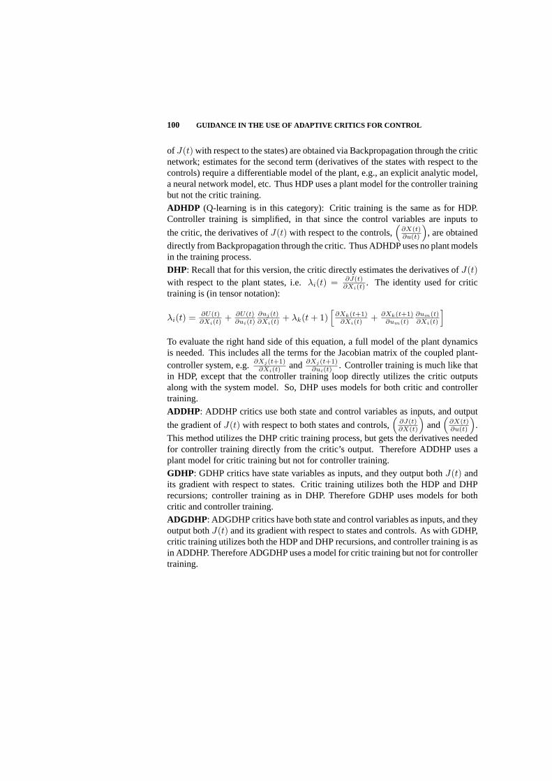
100 GUIDANCE IN THE USE OF ADAPTIVE CRITICS FOR CONTROL
of J(t) with respect to the states) are obtained via Backpropagation through the criticnetwork; estimates for the second term (derivatives of the states with respect to thecontrols) require a differentiable model of the plant, e.g., an explicit analytic model,a neural network model, etc. Thus HDP uses a plant model for the controller trainingbut not the critic training.
ADHDP (Q-learning is in this category): Critic training is the same as for HDP.Controller training is simplified, in that since the control variables are inputs to
the critic, the derivatives ofJ(t) with respect to the controls,(
∂X(t)∂u(t)
), are obtained
directly from Backpropagation through the critic. Thus ADHDP uses no plant modelsin the training process.
DHP: Recall that for this version, the critic directly estimates the derivatives ofJ(t)with respect to the plant states, i.e.λi(t) = ∂J(t)
∂Xi(t). The identity used for critic
training is (in tensor notation):
λi(t) = ∂U(t)∂Xi(t)
+ ∂U(t)∂ui(t)
∂uj(t)∂Xi(t)
+ λk(t + 1)[
∂Xk(t+1)∂Xi(t)
+ ∂Xk(t+1)∂um(t)
∂um(t)∂Xi(t)
]
To evaluate the right hand side of this equation, a full model of the plant dynamicsis needed. This includes all the terms for the Jacobian matrix of the coupled plant-controller system, e.g.∂Xj(t+1)
∂Xi(t)and ∂Xj(t+1)
∂ui(t). Controller training is much like that
in HDP, except that the controller training loop directly utilizes the critic outputsalong with the system model. So, DHP uses models for both critic and controllertraining.
ADDHP: ADDHP critics use both state and control variables as inputs, and output
the gradient ofJ(t) with respect to both states and controls,(
∂J(t)∂X(t)
)and
(∂X(t)∂u(t)
).
This method utilizes the DHP critic training process, but gets the derivatives neededfor controller training directly from the critic’s output. Therefore ADDHP uses aplant model for critic training but not for controller training.
GDHP: GDHP critics have state variables as inputs, and they output bothJ(t) andits gradient with respect to states. Critic training utilizes both the HDP and DHPrecursions; controller training as in DHP. Therefore GDHP uses models for bothcritic and controller training.
ADGDHP: ADGDHP critics have both state and control variables as inputs, and theyoutput bothJ(t) and its gradient with respect to states and controls. As with GDHP,critic training utilizes both the HDP and DHP recursions, and controller training is asin ADDHP. Therefore ADGDHP uses a model for critic training but not for controllertraining.

SOME CURRENT RESEARCH ON ADAPTIVE CRITIC TECHNOLOGY 101
Table I. Summary of requirement for model in training loops
ADP Model NEEDED for training of
STRUCTURE CRITIC CONTROLLER
HDP X
ADHDP
DHP X X
ADDHP X
GDHP X X
ADGDHP X
4.5 SOME CURRENT RESEARCH ON ADAPTIVE CRITICTECHNOLOGY
As part of providing guidance to prospective users of the ADP methods to developcontroller designs, we sketch some of the work being done in the area, and providecitations that the reader may find useful.
Andersen and his colleagues at Colorado State University have been working on com-bining Robust control theory with reinforcement learning methodologies to developproofs for both, static and dynamic stability, (e.g. [1, 2]). A reinforcement learningprocedure has resulted which is guaranteed to remain stable even during training. Inan attempt to speed up the process (which turns out being on the slow side), work isunderway to use predicted reinforcement along with received reinforcement.
Balakrishnan and his colleagues at the University of Missouri-Rolla, have beenworking on applying adaptive critic based neurocontrol for distributed parametersystems (e.g. [11, 12, 26, 36, 37, 38]). The objectives of this research are to developand demonstrate new adaptive critic designs, and to analyze the performance of theseneurocontrollers in controlling parabolic, hyperbolic, and elliptic systems.
Barto and his colleagues at the University of Massachusetts, have been working onmethods to allow an agent learning through reinforcement learning to automaticallydiscover subgoals (e.g. [28, 40]). By creating and using subgoals, the agent is ableto accelerate its learning on the current task, and to transfer its expertise to otherrelated tasks. Discovery of subgoals is attained by examining commonalities acrossmultiple paths to a solution. The task of finding these commonalities is cast as amultiple-instance learning problem, and the concept of diverse density is used to findthe solution.
KrishnaKumar at the NASA Ames Intelligent Flight Controls Lab, and Neighoefer,at Accurate Automation Coorporation, show an interesting implementation and ap-plication of adaptive critics ([14]). The basic idea is that if a nonlinear system can

102 GUIDANCE IN THE USE OF ADAPTIVE CRITICS FOR CONTROL
be linearized at representative points in the operational envelope, then the solution tothe Ricatti equation at each point can be used as the Bellman Value function (“costto go”) for DP. If the Ricatti solutions also show a degree of statistical correlation,then an “Immunized” scheme (which mimics the building block scheme of biologicalimmune systems) can be used with Ricatti solutions as “building blocks” to act asHDP Immunized Adaptive Critics (IAC).
Lendaris and his colleagues at the Portland State University NW ComputationalIntelligence Laboratory (NWCIL) have focused the past few years on exploringapplication issues related to ADP, in particular, the DHP version (e.g. [18, 19, 21,22, 23, 24, 25, 48, 49, 50, 51, 52, 53]). Much of the material reported in this chapteris an outgrowth of that work. A MATLAB based DHP computational platform hasbeen developed, and is available for downloading and use from the NWCIL Web site:www.nwcil.pdx.edu. Key recent research and application results related to ADPinvolve the use of Fuzzy Logic structures for the controller, critic, and/or plant in theDHP ADP method (see Section 4.6.10). A recent application project is the designof a nonlinear controller for a hypersonic-shaped aircraft known as LoFlyter© [20].Current work focuses on exploring methods ofJ∗ surface generation for fast optimaldecision/control design.
Prokhorov and his colleagues at the Ford Research Laboratory have done a significantamount of work in developing stability analysis techniques for neural networks (e.g.,[3, 4, 10]). An interesting application of the AC method was their experiment witha “real” ball and beam system. The benchmark ball and beam system was built inthe lab, and different approaches were used to control the system. Neural networkswere used in three roles: 1) to identify the system, 2) for the controller, and 3) for thecritic. In one of their studies, they made the problem even more difficult by applyinga sticky adhesive to the surface of the beam [9]; the ACs successfully handled theproblem.
Saeks and his colleagues at Accurate Automation Corporation have been workingwith a variety of AC and adaptive dynamic programming implementations (e.g.[30, 45, 46]). Some of these implementations include an ADP algorithm baseddirectly on the Hamilton-Jacobi-Bellman equation, and includes a continuous timestability proof that remains valid during on-line training. In [30], demonstrationsof this algorithm are given for i) the linear case, ii) the nonlinear case using alocally quadratic approximation to the value functional, and iii) the nonlinear caseusing a (potentially global) radial basis function approximation of the Value function.Another AC implementation has been developed suitable for real-time applications[32, 33]. This is a time-varying linear critic methodology based on LQR theory.Applications of these algorithms have included controlling the hybrid power systemof a hybrid electric vehicle, pitch control in simulated aircraft problems, simulated X-43 autolanding analysis, path-planning for autonomous UAV flight, and the guidancemodule of a satellite formation flying algorithm.
Active work is also being performed by researchers such as Paul Werbos, JennieSi, Sylvia Ferrari/Robert Stengel, and Ganesh Venayagamourthy/Donald Wunsch.Please refer to their respective chapters in this book for a summary of their work.
APPLICATION ISSUES 103
4.6 APPLICATION ISSUES
In this section, we discuss various considerations that are important to theapplicationof ADP. Before getting to the specifics, we comment that two major issues confrontedin establishing practical training protocols are (1) the choice of control scenarios,and (2) the setting of values for the different parameters that govern the dynamicsof the learning process. The control scenarios aspect includes the selection ofregulation points, targets/target trajectories, initial plant states, noise regimes, andreset conditions (i.e. when should a training run be terminated). Training parametersof critical importance include the learning coefficients for both the critic and thecontroller, and the discount factorγ used in the Bellman recursion.
4.6.1 Problem Formulation
The mathematical formalism used in previous sections indicates that the plant’s statevector X(t) is input to the critic and to the controller. An important pragmatic issueturns out beingwhat to include in the definition ofX(t) for ADP computational pur-poses? The control engineer using this methodology must have deep understandingof the problem context and the physical plant to be controlled to successfully makethe requisite choices forX(t). A strong suggestion is to invoke your engineeringintuition and whatever rigorous knowledge is available to satisfy yourself that thevariables you select as inputs to the controller and critic are sufficient to assure thatat every point in the corresponding state space, there will exist a unique action for thecontroller to take. If you decide such uniqueness is questionable, then you may haveto estimate some (even a hybrid) variable that will make the state space unique. If thisis not achieved, all is not lost, but more complex learning structures, e.g., recurrentneural networks, may have to be used, and these are more difficult to train.
Not all mathematically describable states are observable; and even if they are inprinciple, there may be instrumentation constraints. Further, there are cases wherewe might be able to measure certain system variables (e.g., acceleration) whereastheory suggests fewer variables (e.g., only position and velocity) are required. But,experience informs us that in some situations, inclusion of the additional measurementcould make the ADP process work better - e.g., if the learning device has to infer theequivalent of acceleration to satisfy certain control objectives, providing accelerationdirectly might be beneficial. However, “more” is not always better, as more inputspotentially add to the computational and inferencing burden. In such a case, onecould explore option(s) equivalent to providing position and acceleration instead ofposition and velocity.
When performing the problem-formulation task, it is useful to discern whether theplant is decomposable - that is, to determine whether certain aspects of the plantdynamics may be considered to be only loosely coupled. If so, this could be usefulwhile crafting the Utility function (discussed below), and even provides the possibilitythat an equivalently loosely decoupled controller architecture might be appropriate.

104 GUIDANCE IN THE USE OF ADAPTIVE CRITICS FOR CONTROL
While it may border on the obvious, another aspect of problem formulation that iscritical to success is a clear statement of the control objectives. Only after clarityof the objectives is at hand, is one in a position to give explicit attention to thefundamental issue of how these objectives are to be represented for ADP application.The choice of this representation is a prerequisite to the next task, and is one of thekey determinants of the eventual success or failure of the ADP design process.
4.6.2 Crafting the Utility Function
The Utility function is the only source of information the ADP process has about thetask for which it is designing the controller. When the statement is made that DynamicProgramming designs anoptimalcontroller, optimality is defined strictly in terms ofthe Utility function. It is important to recognize that a different Utility function will(typically) yield a different controller. The two key creative tasks performed by theuser of ADP are
1. deciding what to include in theX(t) vector, as discussed in the above sub-section,
2. crafting the Utility function in a manner that properly captures/embodies theproblem-domain requirements, and yields a desirable controller.
One mathematical formalism suggests designating the control task in terms of areference trajectory, sayX∗(t) (which could in principle be obtained from a referencemodel), and defining the Utility function directly asU(t) = ||X(t) −X∗(t)|| (e.g.,see [41]). In practice, however, one finds that the ADP process can often be improvedby treating some of the components ofX(t) in a non-uniform manner withinU(t).For example, different relative weightings might be used for various components,or more dramatically, some of the error components might use different powers, oralternatively, have nonlinear coefficients (e.g., see [21, 42]). Further, as suggestedin [16] and [23], there is often substantial benefit to paring downU(t) to containthe minimum number of terms necessary to accomplish the task (what these are,however, are not always easy to determinea priori).
We reproduce here a sequence of Utility functions reported in [21] that were craftedto represent an increasing set of constraints stipulated in the problem definition phase.The context was to design a steering and velocity controller for a 2-axle, terrestrial,autonomous vehicle; the task was to change lanes on a multi-lane road.
The first Utility function defined in that paper is an example of the suggestion abovethat it may be appropriate to have different weightings of the state variables:
U1 = −(
12yerr
)2
−(
18verr
)2
− 116
(v)2
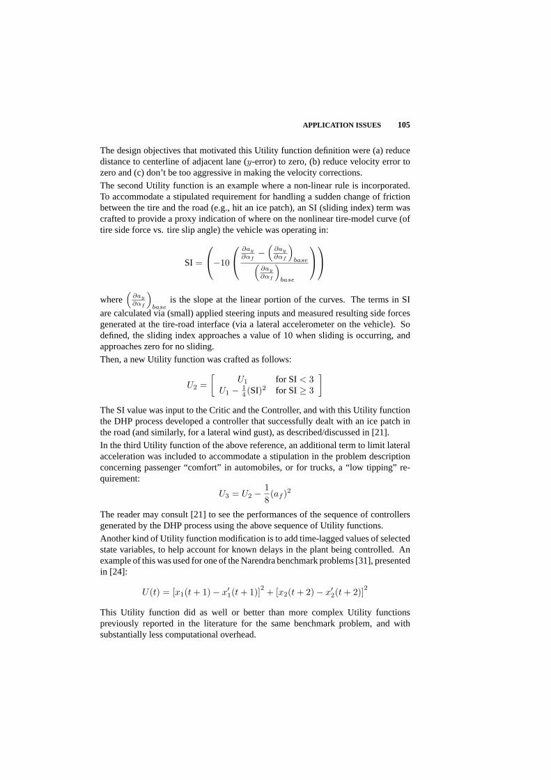
APPLICATION ISSUES 105
The design objectives that motivated this Utility function definition were (a) reducedistance to centerline of adjacent lane (y-error) to zero, (b) reduce velocity error tozero and (c) don’t be too aggressive in making the velocity corrections.
The second Utility function is an example where a non-linear rule is incorporated.To accommodate a stipulated requirement for handling a sudden change of frictionbetween the tire and the road (e.g., hit an ice patch), an SI (sliding index) term wascrafted to provide a proxy indication of where on the nonlinear tire-model curve (oftire side force vs. tire slip angle) the vehicle was operating in:
SI =
−10
∂ay
∂αf−
(∂ay
∂αf
)base(
∂ay
∂αf
)base
where(
∂ay
∂αf
)base
is the slope at the linear portion of the curves. The terms in SI
are calculated via (small) applied steering inputs and measured resulting side forcesgenerated at the tire-road interface (via a lateral accelerometer on the vehicle). Sodefined, the sliding index approaches a value of 10 when sliding is occurring, andapproaches zero for no sliding.
Then, a new Utility function was crafted as follows:
U2 =[
U1 for SI < 3U1 − 1
4 (SI)2 for SI≥ 3
]
The SI value was input to the Critic and the Controller, and with this Utility functionthe DHP process developed a controller that successfully dealt with an ice patch inthe road (and similarly, for a lateral wind gust), as described/discussed in [21].
In the third Utility function of the above reference, an additional term to limit lateralacceleration was included to accommodate a stipulation in the problem descriptionconcerning passenger “comfort” in automobiles, or for trucks, a “low tipping” re-quirement:
U3 = U2 − 18(af )2
The reader may consult [21] to see the performances of the sequence of controllersgenerated by the DHP process using the above sequence of Utility functions.
Another kind of Utility function modification is to add time-lagged values of selectedstate variables, to help account for known delays in the plant being controlled. Anexample of this was used for one of the Narendra benchmark problems [31], presentedin [24]:
U(t) = [x1(t + 1)− x′1(t + 1)]2 + [x2(t + 2)− x′2(t + 2)]2
This Utility function did as well or better than more complex Utility functionspreviously reported in the literature for the same benchmark problem, and withsubstantially less computational overhead.

106 GUIDANCE IN THE USE OF ADAPTIVE CRITICS FOR CONTROL
4.6.2.1 Decomposition of Utility Functions. If during the Problem Formulationtask it is determined that the plant is (even approximately) decomposable, then thereis a potential for crafting separate Utility functions for each of the resulting “chunks.”
In this case, it may be appropriate to define the overall Utility function as a sum ofsuch component Utility functions, i.e.,U(t) = U1(t) + ... + Up(t).With such a formulation, a separate critic estimator could be used for each term. ForHDP critics, one has
J(t) =∞∑
i=0
γiU(t + i)
=∞∑
i=0
p∑
j=1
γiUj(t + i)
=p∑
j=1
Jj(t)
and for DHP
∇J(t) =p∑
j=1
∇Jj(t)
In practice, this decomposition tends to speed up critic learning, as each sub-critic isestimating a simpler function.
In the case of multiple outputs from the controller, the controller learning processcan also be simplified if the additive terms in the cost function correspond to separatemodes, and the latter are dominated by distinct control variables. For example,consider a two dimensional nonlinear system:
x1 = f1(x, u1)
x2 = f2(x, u2)
with primary cost function
U(t) = g1(x, u1, t) + g2(x, u2, t)
and secondary cost function
J(t) = J1(t) + J2(t)
In DHP this could be approached using two critics, each estimating∇J1(t) or∇J2(t)respectively. The complete gradient for controller training would be
(∂
∂u1J1(t) +
∂
∂u1J2(t),
∂
∂u2J1(t) +
∂
∂u2J2(t)
)

APPLICATION ISSUES 107
For initial training, the cross terms could be dropped and the following approximation
used:(
∂∂u1
J1(t), ∂∂u2
J2(t))
. This simplifies the learning of the dominant plant
dynamics and control effects. It may be useful to include a subsequent fine tuning ofthe controller via inclusion of the cross terms, unless the interactions arevery weak.
See [22] for an example of decomposed utility functions for the steering and speedcontrol of a 2-axle terrestrial vehicle. Also, see [41] for a related kind of criticdecomposition, one the author calls ‘primitive adaptive critics.’
4.6.3 Scaling Variables
While theory does not speak to this issue directly, empirical evidence suggests thatit is eminently useful to scale the components ofX(t) being fed into the controllerand the critic (e.g., see [17]), such that each of the variable values are nominally inthe range of±1, particularly when the critic and/or controller are implemented vianeural networks (this recommendation is dependent on the approximating structureused). Further, as indicated above, it is important to pay attention to the relativescaling of the component terms in the Utility function. The latter may hinge solelyon engineering intuition related to the problem domain and the control specifications.
4.6.4 Selecting the Discount Factor
The original equation defined by Bellman that led to Eq. 4.1 above is as follows:
J(t) = U(t) +∞∑
k=1
γkU(t + k) (4.2)
We notice that the Value functionJ(t) is given in terms of the currentU(t), plusthe sum of all future values ofU(·), pre-multiplied by a discount factorγ, where0 ≤ γ ≤ 1. At γ = 0, only the present value ofU is used, ignoring all future values.At γ = 1, all future values are deemed equally important (“infinite horizon” version).
In principle, we might expect theγ value to be governed by the requirements of theoriginal problem formulation. In applying ADP, however, an important issue is howthe value ofγ influences the ADP convergence process (via its role in the Bellmanrecursion, Eq. 4.1). The degree to which this is felt is different for the HDP, DHP, andGDHP structures. To help inform your intuition about this, note that the critic outputsvalues that are used to train itself, so at early stages of the process, the component inEq. 4.1 contributed by the critic may be considered equivalent to ‘noise.’
For the HDP structures, those that directly estimateJ(t) values, appropriatelyselectingγ is critical for convergence of critic training. Common practice (e.g. [9])is to start training with lowγ values and then anneal them up (progressively incrementthem). The lowγ values represent a high discount rate that cancels out the right handterm of the Bellman recursion. This results in the critic learning to approximate(just) the primary utility functionU(t). Progressively incrementingγ then causes the

108 GUIDANCE IN THE USE OF ADAPTIVE CRITICS FOR CONTROL
critic to learn how the primary costs accumulate through time to form the long-term(secondary) value function,J(t).For the DHP structures, those that directly produce∇J(t), this annealing processtends to be less necessary, often allowing largeγ values to be used from the verybeginning. For higher dimensional problems, however, even for the DHP structure, ithas been found useful to “schedule” theγ values. A reasonable rule of thumb is thateven if a larger value ofγ is suggested by the problem formulation and/or the ADPstructure type, use a small value at the early stages of the ADP process, while the stateof knowledge in the critic is low, and as the critic’s training proceeds, incrementallyincreaseγ to higher levels.
4.6.5 Selecting Learning Rates
As mentioned earlier, the ADP structures addressed here all include two trainingloops: one for the critic and one for the controller. Aseparate learning rate(orlearning-rate schedule) is associated with each training loop. In certain special cases,theory may be invoked to determine approximate desired values for the learningrates. For example, in Prokhorov et al., [57], success was reported using dualKalman filters to automatically adjust certain parameters, though this approach addssubstantial computation to the process. More generally, however, “rule of thumb” isour primary guide, and even these are determined empirically within given problemcontexts. Determining the values of these and other parameters turns out being themost labor-intensive aspect of employing the ADP methodology. In some cases, theuser gets the feeling that the process requires an exhaustive search. The NWCIL DHPcomputational platform mentioned in Section 4.5 (available at www.nwcil.pdx.edu)provides a capability to experiment with lots of parameter values with minimal humanintervention.
As is well known, the learning rate values mentioned above are important determi-nants of the training loop dynamics - and in particular, whether or not the processwill converge, and if so, the convergence rate. Pragmatically, one determines usefulranges for the two learning rates empirically. Fortunately, once values are found thatresult in a convergent ADP process, these values are relatively robust to other processparameter changes the user may wish to explore. As with theγ values of the previoussection, once useful ranges for learning rates are found, annealing (scheduling) thelearning rates is also beneficial. The direction of annealing/scheduling in this caseis the opposite: start with larger learning rates, and anneal downwards as learningprogresses.
During the process of discovering useful values of the learning rates, if a selectedset of rates results in the ADP process converging, but very slowly, then increase thelearning rates incrementally - until one or both of the incremented values causes theprocess to diverge. Then just back down a notch or two. The more usual situation,however, is that early experiments result in a divergent process; in these cases, it isuseful to observe which loop diverges first. The rate in this loop is adjusted first. In-tuitively, since the controller is designed based on information acquired by the critic,

APPLICATION ISSUES 109
it would make sense to use a larger learning-rate for the critic (to have it learn faster)than the controller. Indeed, there is empirical evidence for this. However, we havealso seen counterexamples, where it worked better for the controller to have a higherlearning rate. The rule-of-thumb we have developed is to start with a ratio of about10:1 for the learning rates, the critic’s being the larger one. Typical learning-ratevalues found useful in the problem domains explored by the first author in the pasthave been between 0.001 to 0.01, and sometimes up to 0.1.
General summary:
Guidance for selection of ADP process parameters is via “rules of thumb”.
ADP parameter-value determination is the most labor-intensive aspect of employingthe methodology.
Specific to this subsection:
Learning rate values determine training loop dynamics.
It is useful to use separate rates in each training loop.
One Rule of Thumb: Use a ratio of about 10:1 for the learning rates, the larger onefor the critic loop (however, see caveat in the text).
To determine useful range(s) for learning rates, start exploration with (sometimesvery) low values to find at least one set that will yield convergence; increase incre-mentally until process no longer converges; then back down a notch or two.
If no combination is found that yields convergence, see next subsection.
Learning-rate values found useful in applications to date (by first author and co-workers) for the critic loop are between 0.001 - 0.01, and sometimes up to 0.1.
Once useful ranges of learning rates are determined, scheduling (annealing) the rateswithin these ranges may be beneficial during the design runs.
Scheduling of Learning Rate values goes from large to small (in contrast to schedulinggamma values of previous sub-section, which goes from small to large).
4.6.6 Convergence of the ADP (controller design) process
The task of getting the ADP process to converge involves a carefully orchestratedselection of all of the above items. Experience indicates that there is strong interactionamong their values in how they affect ADP convergence. If after scaling has beenaccomplished and exploration of learning rate andγ values has been performed withno successful convergence, we suggest reconsidering the Utility function formulation.We have examples of situations where seemingly minor changes in the formulation ofthe Utility function resulted in dramatically different ADP convergence behavior andresulting controller design. Associated with this, it may also be useful to reconsiderthe selection of variables being used as inputs to the controller and to the critic (cf.discussion in Section 4.6.1 as well).

110 GUIDANCE IN THE USE OF ADAPTIVE CRITICS FOR CONTROL
4.6.7 Designing the Training “Syllabus”
Specific attention must be given to the design of the training regimen. Many issuesneed to be considered. In the control context, a key issue ispersistence of excitation,which entails a requirement that the plant be stimulated such that all important modesare excited “sufficiently often” during the learning process. Additionally, it is alsoimportant that the full range of controller actions are experienced. A key rule-of-thumb in designing the regimen is to start the training with the simplest tasks first,and then build up the degree of difficulty. The truck backer-upper project of [35]provides an excellent example of this training principle, albeit in the context of adifferent learning methodology (Backpropagation through time).
The above rule-of-thumb includes considerations such as choosing initial plant statesnear regulation points or target states, selecting target trajectories that remain withina region of state space with homogenous dynamics, and initializing the controllerwith a stabilizing control law. This last approach falls under the topic of usingapriori information to pre-structure either the controller or critic (more on this below).As the easier scenarios are successfully learned, harder scenarios are introduced ina manner that persistence of excitation across the entire desired operating region isachieved. In this stage, initial conditions for the plant are chosen farther and fartherfrom regulation points, target trajectories are chosen so as to cross boundaries inqualitative dynamics, etc. The progression continues until the entire operating rangeof the controller is being exercised in the training runs.
A useful practice employed by the authors is to brainstorm how we would trainanimals or humans, including ourselves, to learn the given task. We then transformthe insights gained into candidate training syllabi for the given ADP task.
4.6.8 Stopping/Reset Criteria
Another operational issue to consider is when to stop the learning process and startover again. In the well-known pole-cart problem, there is a straightforward decision:When the pole drops, stop the process, reset the pole, and continue the training process(e.g. see [16, 17]). As another example, consider training a steering controller fora 4-wheeled terrestrial vehicle to change lanes on a highway: if the vehicle goesoff the road, rather than continuing the training process to see if the controller canlearn to get the vehicle back on the highway, instead, stop the process as soon as thevehicle goes “out of bounds,” return to the starting point, and continue the training,starting the controller and critic weights (in the NN context) where they left off (e.g.,see [21, 22]). The idea is to give an opportunity to improve the controller based onthe design it had just before going out-of-bounds, rather than after it got “mired inthe mud,” as it might do in attempting to get back on the highway in the steeringexample. This idea may easily be generalized: Specify limits for each componentof X(t) (andu(t) if appropriate) being used in the Utility function, create an out-of-bounds monitoring procedure, when an out-of-bound condition is detected (for one

APPLICATION ISSUES 111
or more of the monitored variables), stop the process, return to an appropriate startingpoint, and continue the training.
This stop/reset strategy may also be usefully applied in those cases where the criticcontinues to diverge, no matter what choices are made with learning rate and/orother parameters. After a relatively “sweet” spot in the parameter values has beendetermined, even if the process does not converge by itself, the stop/reset strategyhas been successfully employed to get the system to converge.
4.6.9 Simultaneous vs. Sequential Operation of Critic and ControllerTraining Loops
Once a forward computation is performed through the controller and plant, and acritic output is obtained (estimate ofJ(t) or its derivatives), the ADP system ispoised to perform a learning cycle in each of the two training loops. One strategywould be to simultaneously perform a learning cycle in both. This strategy works,and indeed, the authors routinely use it. However, experimentally determining valuesfor the ADP process parameters discussed above is sometimes more difficult with thisstrategy than with other possibilities. In some early papers (e.g. [42, 43, 47, 57, 60],a “flip-flop” strategy was proposed wherein training was performed a number oftimes (called an epoch) in one loop while the training for the other loop was puton “hold”, and then during the next epoch, the roles of being trained and being onhold were flipped. This flip-flop sequencing continued until the whole ADP processconverged. While this strategy tends to be easier to get to converge, its convergencerate is slower than for other alternatives. This slower convergence is a consequenceof losing information in those loops that are placed on hold. Additional strategieswere subsequently developed (see [16, 17]) that also make use of the principle ofseparate (non-simultaneous) training, but in addition provide a means of preservingall the available information, thus avoiding the penalty of longer convergence times.The mechanism for preserving the information is called “shadow critic” in the critictraining loop, and “shadow controller” in the controller training loop. The shadowconcept entails performing the training updates in a COPY of the critic (rather thanin the critic itself) and in a COPY of the controller during their respective “hold”epochs. Then at the end of the “hold” epoch, the design in the COPY (shadowversion) is uploaded to the in-line version as a starting point for training duringthe next epoch. Various combinations are described: Shadow Critic Only; ShadowController Only; Shadow Critic and Shadow Controller. The motivating benefitfor using these alternate strategies is their enhanced convergence performance. Inaddition, however, for some limited cases explored, the controller designs generatedvia the various strategies had some qualitative differences as well [24].
More recently, the Shadow Controller concept was incorporated in a proposed designof a method to deal with stability issues that arise when the ADP method is to beused in an on-line context [19]. See Section 4.6.11 below.
112 GUIDANCE IN THE USE OF ADAPTIVE CRITICS FOR CONTROL
4.6.10 Embedding a-priori Knowledge
If a priori knowledge is available about the problem domain that may be translatedinto a starting design of the controller and/or the critic, then it behooves us to use thisknowledge as a starting point for the ADP procedures. While the ADP methods maybe made to converge with random initializations of the controller and critic networks(usually only applicable in off-line situations), it is generally understood that thebetter the starting controller design, the “easier” it will be for the ADP process toconverge. Another way to look at this is that if the starting controller design is “close”to an optimal design (e.g., the human designers already did a pretty good job), thenthe ADP system’s task is one ofrefininga design - and this is intuitively easier thanhaving to explore the design domain to even get to what is astarting point in theassumed context.
There are a variety of ways to obtaina priori information about the problem domainthat can be used to initialize the trainable function approximator in the ADP process.For example, consider a system with an existing controller, but the controller’s designis known to be non-optimal and it is desired to improve the design. One could traina neural network to copy this controller, substitute this NN in place of the controller,and implement an ADP process to optimize the controller design. If the ADP requiresa differentiable plant model, then such a model will also have to be developed beforestarting the process. With this starting controller design, one would begin the ADPprocess with a long epoch to train just the critic, and then transition into one of thestrategies described in the previous section to incrementally improve both, the critic’sestimate ofJ∗ and the corresponding controller design.
An alternate location to embeda priori knowledge is in the critic. For example, inthe context of an LQR (linear quadratic regulator) problem, theJ∗ surface is knownto be parabolic. While the various parameter values of the parabolic surface may notbe known a priori, if the critic is pre-structured to just represent such surfaces, thenADP convergence is enhanced, e.g. see [54]. We think of this in terms of pre-biasingthe critic’s ‘perception’ of the problem.
Often times, the key source ofa priori knowledge resides in the head of a humanexpert. There is little available in the neural network literature that provides guidanceon how to embed such a priori knowledge into a neural network starting design. Onthe other hand, a large literature has developed in recent decades describing theoryand methods for using Fuzzy Logic to capture such human expertise, and further, forusing Fuzzy Systems in the controls context. Space limitations preclude surveyingthat literature here; a couple of accessible suggestions to the reader are [58, 62]. It isimportant to point out here that certain Fuzzy structures qualify as trainable universalfunction approximators, and thus, should in principle be usable in ADP processes.Indeed, successful use of Fuzzy structures for both controller and/or critic roles,and in fact, for the plant’s differentiable model, have been accomplished (e.g., see[50, 51, 53]). We summarize below an example of such an application (taken from[50]), to convey the thought process you would use to employ such techniques. A
APPLICATION ISSUES 113
summary of the results to be described in the following few paragraphs is given inTable II.
A Fuzzy structure known as a first-order TSK model (e.g. see [62]) offers a directapproach for representing the relevant characteristics of the plant, and for prestructur-ing both the controller and critic. A very simple model of the well-known cart-polesystem was constructed using such a structure, and for DHP training, it was demon-strated that this model’s effectiveness was comparable to the use of a full analyticmodel. This is especially interesting since no example-specific information (polelength or mass, cart mass, etc.) was included in the model.
The line of reasoning went as follows. First, it was noted that the six observable vari-ables (related to pole angleθ and cart positionx) constitute a coupled pair of second or-der systems. It can be inferred that the derivatives∂θ
∂θ , ∂θ∂θ
, ∂θ∂θ
, ∂θ∂θ
, ∂θ∂θ
, ∂x∂x , ∂x
∂x , ∂x∂x , ∂x
∂x
and ∂x∂x are all always positive. This observation constitutes a partialqualitative
modelof the plant’s dynamics. An additional observation is that application of apositive control force to the cart tends to increasex, x andx, and decreaseθ, θ andθ; this a priori knowledge allows setting∂x
∂u , ∂x∂u , and ∂x
∂u positive, and∂θ∂u , ∂θ
∂u and∂θ∂u negative. This collection ofassumptionswas defined as the Double IntegratorModel (DIM). When the DIM was substituted into the baseline DHP training proce-dure in place of the true analytic plant model, the procedure successfully produceda controller81 percent of the time (as compared to 99.99 percent with the analyticmodel).
Buoyed by this promising result, another piece ofa priori knowledge was crafted outof the observable fact that when the pole is deflected from vertical, the force of gravitywill tend to increase the angular acceleration of the pole in the same direction as thedeflection while also imparting an acceleration to the cart in the opposite direction.This resulted in a new pair of rules:
If θ 6= 0 then∂x
∂θis negative
and
If θ 6= 0 then∂θ
∂θis positive
The DIM augmented with these two rules was called the Crisp Rule Double IntegratorModel (CRDIM). When used in the DHP training procedure this model turned outbeing only 76 percent effective.
While initially disappointing, this result provided the context for an important con-clusion: while the linguistic description of the plant’s behavior is correct, thecrispimplementationof the rules that were used actually detracted from the effectivenessof the CRDIM for controller training. By moving to a Fuzzy framework for theentiremodel, substantially improved results were obtained.
To keep the fuzzy implementation simple, only three linguisticvalueswere usedfor each variable: POSITIVE, ZERO and NEGATIVE. A triangular membershipfunction was used for the ZERO linguistic value (with end points scaled consistent
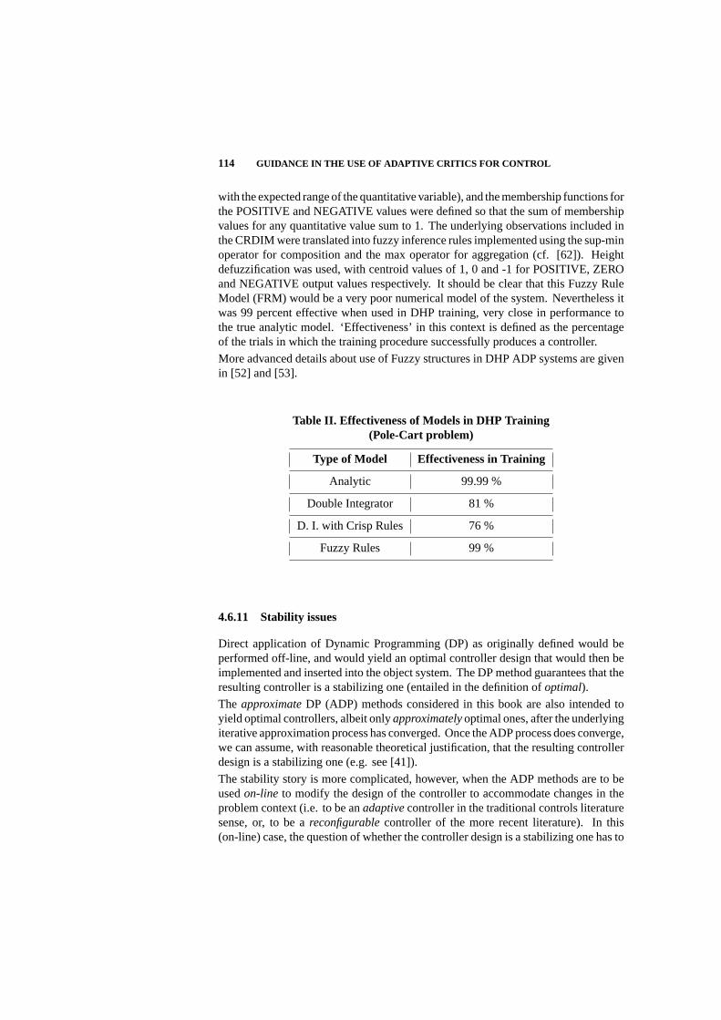
114 GUIDANCE IN THE USE OF ADAPTIVE CRITICS FOR CONTROL
with the expected range of the quantitative variable), and the membership functions forthe POSITIVE and NEGATIVE values were defined so that the sum of membershipvalues for any quantitative value sum to 1. The underlying observations included inthe CRDIM were translated into fuzzy inference rules implemented using the sup-minoperator for composition and the max operator for aggregation (cf. [62]). Heightdefuzzification was used, with centroid values of 1, 0 and -1 for POSITIVE, ZEROand NEGATIVE output values respectively. It should be clear that this Fuzzy RuleModel (FRM) would be a very poor numerical model of the system. Nevertheless itwas 99 percent effective when used in DHP training, very close in performance tothe true analytic model. ‘Effectiveness’ in this context is defined as the percentageof the trials in which the training procedure successfully produces a controller.
More advanced details about use of Fuzzy structures in DHP ADP systems are givenin [52] and [53].
Table II. Effectiveness of Models in DHP Training(Pole-Cart problem)
Type of Model Effectiveness in Training
Analytic 99.99 %
Double Integrator 81 %
D. I. with Crisp Rules 76 %
Fuzzy Rules 99 %
4.6.11 Stability issues
Direct application of Dynamic Programming (DP) as originally defined would beperformed off-line, and would yield an optimal controller design that would then beimplemented and inserted into the object system. The DP method guarantees that theresulting controller is a stabilizing one (entailed in the definition ofoptimal).
The approximateDP (ADP) methods considered in this book are also intended toyield optimal controllers, albeit onlyapproximatelyoptimal ones, after the underlyingiterative approximation process has converged. Once the ADP process does converge,we can assume, with reasonable theoretical justification, that the resulting controllerdesign is a stabilizing one (e.g. see [41]).
The stability story is more complicated, however, when the ADP methods are to beusedon-line to modify the design of the controller to accommodate changes in theproblem context (i.e. to be anadaptivecontroller in the traditional controls literaturesense, or, to be areconfigurablecontroller of the more recent literature). In this(on-line) case, the question of whether the controller design is a stabilizing one has to
APPLICATION ISSUES 115
be askedat each iterationof the ADP design process. This is calledstepwisestabilityin [30] or staticstability in [2].
As in Section 4.5, we offer here a brief review of related research (here concerningstability issues) as part of providing guidance to prospective users of the ADP.
4.6.11.1 Recent Approaches to Stability IssuesThe group at Colorado StateUniversity address the issue of stability in ADP systems in terms of what they call‘static’ stability and ‘dynamic’ stability, [2]. Their static stability means that each timethe controller’s design is modified, it continues to be a stabilizing controller. This kindof stability is called step-wise stability in [30]. Theirdynamicstability notion, on theother hand, refers to the dynamics introduced by the sequence of changed controllerdesigns in the loop. They approach static stability with neural network controllers byfirst extracting the linear time-invariant (LTI) components of the neural network andrepresenting the remaining parts as sector-bounded nonlinear uncertainties. IntegralQuadratic Constraint (IQC) analysis [1] is then used to determine the stability of thesystem consisting of the plant, nominal controller, and the neural network with givenweight values. The dynamic stability problem is addressed by once again treating theneural network’s nonlinear components as sector bounded nonlinear uncertainties.In addition, uncertainty in the form of a slowly time-varying scalar is added tocover weight changes during learning. Finally, IQC analysis is applied to determinestability [29]. In this way, the network weight learning problem is transformed intoone of network weight uncertainty; following this, a straightforward computationguarantees the stability of the network during training. The “down side” of thisapproach is its rather slow convergence to a design solution.
The group at the University of Massachusetts uses Lyapunov methods to success-fully verify qualitative properties of controller designs, such as stability, or limitingbehavior, [28]. Lyapunov-based methods are used to ensure that an agent learningthrough reinforcement learning exhibits behavior that satisfies qualitative propertiesrelating to goal-achievement and safety.
The group at the Ford Research Laboratories has done a significant amount of work inanalyzing the stability of recurrent neural networks (RNNs), [3, 4, 9, 10]. Their workfocuses on the global Lyapunov stability of multilayer perceptrons, where they assumethe network weights are fixed. They perform a state space transformation to convertthe original RNN equations to a form suitable for stability analysis. Then appropriatelinear matrix inequalities (LMI) are solved to determine whether the system understudy is globally exponentially stable. In [4], an on-line system capable of analyzingan input-output data sequence to construct a sequence of binary classifications withoutbeing provided correct class information as part of the training process is described.The system employs both supervised and unsupervised training techniques to formmultiple behavior models.
The group at Portland State University’s NW Computational Intelligence Laboratoryhas proposed a computation/simulation approach based on the Shadow Controllerconcept mentioned in Section 4.6.9 (e.g. see [18, 19]). This approach is predicted tobecome viable for on-line applications as computational power continues to increase.
116 GUIDANCE IN THE USE OF ADAPTIVE CRITICS FOR CONTROL
Since the issue during on-line training of a controller is to avoid instantiating intothe control loop a controller that is not stabilizing, the (DHP, in their case) trainingis done only on the Shadow Controller. While many issues remain to be resolved forthis proposed procedure, the idea is to determine the (local) stability of the currentShadow Controller design by performing a high-speed simulation of the closed loop(using the plant model already required for the DHP method), determine a locallinearization, determine the s-plane pole locations, and from this test to determinewhether the current Shadow Controller design meets minimum stability requirements;if so, upload the design to the on-line controller; if not, wait until another train/testcycle. The assumption is that stabilizing controller designs will occur sufficientlyoften to render the proposed procedure viable.
The group at Accurate Automation Corporation has developed an adaptive dynamicprogramming (incidentally, in [30], the acronym ADP is used for Adaptive DynamicProgramming, whereas in the present book ADP is used for Approximate DynamicProgramming) algorithm with a continuous time stability proof, [30] . The algorithmis initialized with a (stabilizing) Value function, and the corresponding control lawis computed via the Hamilton-Jacobi-Bellman Equation (which is thus guaranteedto be a stabilizing controller for this step), and the system is run; the resultant statetrajectories are kept track of and used to update the Value function in a soft computingmode. The method is repeated to convergence. In [30], this method is shown to beglobally convergent, with step-wise stability, to the optimal Value function / controllaw pair for an (unknown) input affine system with an input quadratic performancemeasure (modulo the appropriate technical conditions). This algorithm has beendemonstrated on the example problems mentioned in Section 4.5 for Saeks and hiscolleagues.
4.7 ITEMS FOR FUTURE ADP RESEARCH
As mentioned in Section 4.1, much progress in the development and application ofAdaptive Critics has already occurred, yet much remains to be done. We com-ment here on two topics that appear to us to have significant potential for ex-panded/enhanced application of the ADP methods. One relates to employmentof Fuzzy communication among the actors in an ADP system, and the other relatesto speeding up the process ofJ∗ generation in selected problem domains.
The idea for the latter is to develop a computational intelligence methodology thatefficiently designs optimal controllers foradditional problemswithin an assumedproblem domain,based on knowledge of existing designs in that domain. Researchon this approach is just starting at the NWCIL, but promises to benefit from broaderinvolvement. As currently envisioned, the key ingredient of this methodology willbe aJ∗ Surface Generator(J∗SG). Fundamental tasks in this quest involve repre-sentation, representation, representation.
The idea for including Fuzzy communication among the actors in an ADP system(in contrast to within the various actors, as discussed in Section 4.6.10) is motivated

ITEMS FOR FUTURE ADP RESEARCH 117
by observing the process wherein, for example, a human athlete refines his/herperformance based on verbal hints/instructions provided by an experienced coach(this may apply to many human activities, such as dancing, art, etc.). A potentiallykey location for receiving/embedding such knowledge communicated via a Fuzzyrepresentation could be the Utility function. A hint that the Utility function could bethe heart of such a refinement process may reside for us in the sequence of additionsto the Utility functions described in Section 4.6.2, and the corresponding refinementsin controller performance achieved. Each of us has many personal experiences ofusing verbally communicated guidance to enhance some kind of performance, andthis could provide a rich source of intuition for such an approach. We encouragedialogue to begin within our research community.
Acknowledgments
Most of the work reported in Sections 4.4 & 4.6 of this chapter was supported by NSF Grant#ECS-9904378, G. Lendaris, PI.

Bibliography
1. C. Anderson. Approximating a policy can be easier than approximating a valuefunction. Technical Report CS-00-101, Colorado State University, 2000.
2. C. Anderson, R. M. Kretchner, P. M. Young, and D. C. Hittle. Robust reinforce-ment learning control with static and dynamic stability.International Journal ofRobust and Nonlinear Control, 11, 2001.
3. N. Barabanov and D. Prokhorov. Stability analysis of discrete-time recurrentneural networks.IEEE Trans. On Neural Networks, March, 2002.
4. N. Barabanov and D. Prokhorov. Two alternative stability criteria for discrete-time rmlp. Las Vegas, NV, Dec. 2002. Control and Decision Conference.
5. A. G. Barto. Handbook of Intelligent Control, chapter Reinforcement Learn-ing and Adaptive Critic Methods, pages 469–491. New York: Van Nostrand-Reinhold, 1992.
6. A. G. Barto and R. S. Sutton.Reinforcement Learning: An Introduction. MITPress, 1998.
7. R. E. Bellman.Dynamic Programming. Princeton University Press, 1957.
8. D. P. Bertsekas and J. N. Tsitsiklis.Neuro-Dynamic Programming. AthenaScientific, 1996.
9. P. Eaton, D. Prokhorov, and D. Wunsch. Neurocontroller for fuzzy ball-and-beamsystems with nonlinear, nonuniform friction.IEEE Trans. On Neural Networks,pages 423–435, March 2000.
10. L. Feldkamp, T. Feldkamp, and D. Prokhorov.Intelligent Signal Processing,chapter An Approach to Adaptive Classification. IEEE Press, 2001.
11. Z. Huang and S. N. Balakrishnan. Robust adaptive critic based neurocontrollersfor missiles with model uncertainties.2001 AAA Guidance, Navigation andControl Conference, Montreal, Canada, Aug 2001.
12. Z. Huang and S.N. Balakrishnan. Robust adaptive critic based neurocontrollersfor systems with input uncertainties.Proceedings of IJCNN’2000, Como, Italy,pages B–263, July 2000.
118

BIBLIOGRAPHY 119
13. L. P. Kaelbling, M. L. Littman, and A. W. Moore. Reinforcement learning: Asurvey.Journal of Artificial Intelligence Research, 4:237–285, 1996.
14. K. KrishnaKumar and J. Neidhoefer. Immunized adaptive critics. invited sessionon Adaptive Critics, ICNN ’97, Houston, 1997. A version of this was presentedat ANNIE ’96, November 10- 13, St. Louis, MO.
15. K. KrishnaKumar and J. Neidhoefer.Immunized Adaptive Critic for an Au-tonomous Aircraft Control Application. Artificial immune systems and theirapplications. Springer-Verlag, Inc., 1998.
16. G. G. Lendaris and T. T. Shannon C. Paintz. More on training strategies forcritic and action neural networks in dual heuristic programming method (invitedpaper). Proceedings of Systems Man and Cybernetics Society InternationalConference’97, Orlando, IEEE Press, October 1997.
17. G. G. Lendaris and C. Paintz. Training strategies for critic and action neuralnetworks in dual heuristic programming method.Proceedings of InternationalConference on Neural Networks’97 (ICNN’97), Houston, 1997.
18. G. G. Lendaris, R. A. Santiago, and M. S. Carroll. Dual heuristic programmingfor fuzzy control.Proceeedings of IFSA / NAFIPS Conference,Vancouver, B.C.,July 2002.
19. G. G. Lendaris, R. A. Santiago, and M. S. Carroll. Proposed framework for apply-ing adaptive critics in real-time realm.Proceedings of International Conferenceon Neural Networks’02 (IJCNN’ 2002), Hawaii, May 2002.
20. G. G. Lendaris, R. A. Santiago, J. McCarthy, and M. S. Carroll. Controller designvia adaptive critic and model reference methods.Proceedings of InternationalConference on Neural Networks’03 (IJCNN’ 2003), Portland, July 2003.
21. G. G. Lendaris and L. J. Schultz. Controller design (from scratch) using approx-imate dynamic programming.Proceedings of IEEE International Symposium onIntelligent Control ’2000,(IEEE-ISIC’2000), Patras,Greece, July 2000.
22. G. G. Lendaris, L. J. Schultz, and T. T. Shannon. Adaptive critic design for intelli-gent steering and speed control of a 2-axle vehicle.Proceedings of InternationalConference on Neural Networks’00 (IJCNN’2000) Italy, Jan 2000.
23. G. G. Lendaris and T. T. Shannon. Application considerations for the dhpmethodology. Proceedings of the International Joint Conference on NeuralNetworks’98 (IJCNN’98), Anchorage, IEEE Press, May 1998.
24. G. G. Lendaris, T. T. Shannon, and A. Rustan. A comparison of training al-gorithms for dhp adaptive critic neuro-control.Proceedings of InternationalConference on Neural Networks’99 (IJCNN’99), Washington,DC, 1999.

120 BIBLIOGRAPHY
25. G. G. Lendaris, T. T. Shannon, L. J. Schultz, S. Hutsell, and A. Rogers. Dualheuristic programming for fuzzy control.Proceeedings of IFSA / NAFIPS Con-ference,Vancouver, B.C., July 2001.
26. X. Liu and S. N. Balakrishnan. Convergence analysis of adaptive critic basedneural networks.Proceedings of 2000 American Control Conference, Chicago,IL, June 2000.
27. R. Luus.Iterative Dynamic Programming. CRC Press, 2000.
28. A. McGovern and A. G. Barto. Automatic discovery of subgoals in reinforcementlearning using diverse density.Proceedings of the 18th International Conferenceon Machine Learning, pages 361–368, 2001.
29. A. Megretski and A. Rantzer. System analysis via integral quadratic constraints:Part ii. Technical Report ISRN LUTFD2/TFRT-7559-SE, Lund Institute ofTechnology, September, June 1997.
30. J. J. Murray, C. Cox, G.G. Lendaris, and R. Saeks. Adaptive dynamic program-ming. IEEE TRANSACTIONS on SYSTEMS, MAN. and CYBERNETICS, PARTC: Applications and Reviews, 32, No.2:140–153, May 2002.
31. K. S. Narendra and S. Mukhopadhyay. Adaptive control of nonlinear multivari-able systems using neural networks.Neural Networks, 7(5):737–752, 1994.
32. J. C. Neidhoefer. Report. Technical Report AAC-01-055, Accurate AutomationCorp, 2001.
33. J. C. Neidhoefer. Report. Technical Report AAC-02-016, Accurate AutomationCorp, 2002.
34. J. C. Neidhoefer and K. Krishnakumar. Intelligent control for autonomous aircraftmissions.IEEE Transactions on Systems, Man, and Cybernetics, Part A, January2001.
35. D. Nguyen and B. Widrow.Neural Networks for Control, chapter The TruckBacker-Upper: an Example of Self Learning in Neural Networks. MIT Press,1957.
36. R. Padhi and S. N. Balakrishnan. Adaptive critic based optimal control fordistributed parameter systems.Proceedings International Conference on Infor-mation, Communication and Signal Processing, December 1999.
37. R. Padhi and S. N. Balakrishnan. A systematic synthesis of optimal processcontrol with neural networks.Proceedings American Control Conference, Wash-ington, D.C., June 2001.
38. R. Padhi, S. N. Balakrishnan, and T. Randolph. Adaptive critic based optimalneuro control synthesis for distributed parameter systems.Automatica, 37:1223–1234, 2001.

BIBLIOGRAPHY 121
39. J. C. Pearce.The Biology of Transcendence. Park Street Press, 2002.
40. T. J. Perkins and A. G. Barto. Lyapunov design for safe reinforcement learning.AAAI Spring Symposium on Safe Learning Agents.
41. D. Prokhorov.Adaptive Critic Designs and their Application. PhD thesis, TexasTech University, 1997. Department of Electrical Engineering.
42. D. Prokhorov, R. Santiago, and D. Wunsch. Adaptive critic designs: A casestudy for neurocontrol.Neural Networks, 8:1367–1372, 1995.
43. D. Prokhorov and D. Wunsch. Adaptive critic designs.IEEE Transactions onNeural Networks, 8(5):997–1007, 1997.
44. A. Rogers, T. T. Shannon, and G. G. Lendaris. A comparison of dhp basedantecedent parameter tuning strategies for fuzzy control.Proceedings ofIFSA/NAFIPS Conference, Vancouver B.C., July, 2001.
45. R. Saeks, C. Cox, J. Neidhoefer, and D. Escher. Adaptive critic control of thepower train in a hybrid electric vehicle.Proceedings SMCia Workshop, 1999.
46. R. Saeks, C. Cox, J. Neidhoefer, P. Mays, and J. Murray. Adaptive critic controlof a hybrid electric vehicle.IEEE Transactions on Intelligent TransportationSystems, 3, No.4, December, 2002.
47. R. Santiago and P. Werbos. New progress towards truly brain-like intelligentcontrol. PROC WCNN ’94, pp. I-2toI-33, Erlbaum, 1994.
48. L. J. Schultz, T. T. Shannon, and G. G. Lendaris. Using dhp adaptive critic meth-ods to tune a fuzzy automobile steering controller.Proceedings of IFSA/NAFIPSConference, Vancouver, B.C., July, 2001.
49. T. T. Shannon. Partial , noisy and qualitative models for adaptive critic basedneuro-control.Proceedings of International Conference on Neural Networks’99(IJCNN’99), Washington, D.C., July, 1999.
50. T. T. Shannon and G. G. Lendaris. Qualitative models for adaptive critic neuro-control. Proceedings of IEEE SMC’99 Conference, Tokyo, June, 1999.
51. T. T. Shannon and G. G. Lendaris. Adaptive critic based approximate dynamicprogramming for tuning fuzzy controllers.Proceedings of IEEE-FUZZ 2000,IEEE Press, 2000.
52. T. T. Shannon and G. G. Lendaris. A new hybrid critic-training method forapproximate dynamic programming.Proceedings of International Society forthe System Sciences, ISSS’2000, Toronto, August, 2000.
53. T. T. Shannon and G. G. Lendaris. Adaptive critic based design of a fuzzy motorspeed controller.Proceedings of ISIC2001, Mexico City, Mexico, September,2001.

122 BIBLIOGRAPHY
54. T. T. Shannon, R. A. Santiago, and G. G. Lendaris. Accelerated critic learning inapproximate dynamic programming via value templates and perceptual learning.Proceedings of IJCNN’03, Portland, July, 2003.
55. S. Shervais and T. T. Shannon. Adaptive critic based adaptation of a fuzzypolicy manager for a logistic system.Proceedings of IFSA /NAFIPS Conference,Vancouver, B.C., July, 2001.
56. R. S. Sutton, A. G. Barto, and R. J. Williams. Reinforcement learning is directadaptive optimal control.Proceedings of the American Control Conference,Boston, MA, pp. 2143-2146, 1991.
57. N. Visnevski and D. Prokhorov. Control of a nonlinear multivariable system withadaptive critic designs.Proceedings of Artificial Neural Networks in Engineering(ANNIE), ASME Press, New York, 6:559–565, 1996.
58. L. X. Wang.A Course in Fuzzy Systems and Control. Prentice Hall, 1997.
59. P. J. Werbos.Neural Networks for Control, chapter A Menu of Designs forReinforcement Learning Over Time, pages 67–95. MIT Press, Cambridge, MA,1990.
60. P. J. Werbos.Handbook of Intelligent Control: Neural, Fuzzy, and Adaptive Ap-proaches, chapter Approximate Dynamic Programming for Real-Time Controland Neural Modeling, pages 493–525. Van Nostrand Reinhold, New York, 1994.
61. B. Widrow, N. Gupta, and S. Maitra. Punish/reward: Learning with a critic inadaptive threshhold systems.IEEE Transactions on Systems, Man and Cyber-netics, 3(5):455–465, 1973.
62. J. Yen and R. Langari.Fuzzy Logic: Intelligence, Control and Information.Prentice Hall, 1999.

5 Direct Neural DynamicProgramming
JENNIE SI and DERONG LIULEI YANGArizona State University University of Illinois at Chicago
Editor’s Summary: This chapter introduces direct neural dynamic programming (di-rect NDP), which belongs to the class of heuristic dynamic programming algorithmsdiscussed in Chapters 3, 19, and 4. However, direct NDP is a model-independentapproach to action-dependent heuristic dynamic programming. It is, therefore, anon-line learning control paradigm. This chapter contains a comparison study usingother well-known algorithms to help readers gain quantitative insight on several ADPalgorithms. It also contains results of direct NDP controlling a triple-link invertedpendulum using many continuous state variables and a continuous control, and di-rect NDP in a wireless network call admission control application. Furthermore,in Chapter 21 direct NDP is demonstrated on an industrial scale Apache helicoptermodel for stabilization, tracking control, and reconfiguration after component failure.Preliminary results indicate that direct NDP has the potential to address large scaleproblems.
5.1 INTRODUCTION
The term reinforcement learning is often used when discussing approximate dynamicprogramming (ADP) in the computer science and machine learning community.Associated with this term is a wide range of solid results obtained both analyticallyand empirically by considering learning in the arena of Markov decision processes[5, 20]. In most of its analyses and applications, reinforcement learning results assumediscrete cases, where the state and action spaces can be enumerated and stored inmemory. Another class of systems, adaptive critic designs, address some very similarissues, namely to develop learning systems that can improve their performance overtime through interactions with the environment and through past experience. Thefoundation of this approach is built on the calculus of variations used in optimal
123

124 DIRECT NEURAL DYNAMIC PROGRAMMING
control theory. The problem construct of adaptive critic designs introduces thepossibility of designing learning systems that can handle continuous state spaceproblems or the possibility of addressing generalization issues and design robustnessissues.
This chapter introduces direct neural dynamic programming (direct NDP). The term“direct” is influenced by the adaptive control literature where “direct adaptive con-trol” means no plant model, and thus no plant parameter estimation takes place butinstead certain plant information is used directly to find appropriate and convergentcontrol laws and control parameters. In direct NDP, two generic (neural) functionapproximators are used to represent both the value function (for control performanceevaluation) and the action function (for control law generation). Furthermore, thestate information is used directly in learning the control law where the controllerparameters are the weight parameters in the action function implemented by a neuralnetwork. Therefore direct NDP is a model-independent approach to action-dependantheuristic programming [25].
The class of adaptive critic designs [22] - [26] encompasses several important ideasand implementations of model-based approximate dynamic programming includingheuristic dynamic programming (HDP), dual heuristic dynamic programming (DHP),and globalized dual heuristic dynamic programming (GDHP). A distinguishing fea-ture of the adaptive critic designs is the potential of addressing large scale problemsincluding continuous state and control problems. Several applications and case stud-ies have been developed to demonstrate the feasibility of some key adaptive criticdesign techniques where globalized dual dynamic programming has been found themost effective in the family as a nonlinear controller (refer to [14, 9] and results inChapter 19). As a model-independent approach to the action-dependent heuristicdynamic programming, the direct NDP is expected to achieve computational effi-ciency and reliability due to its simple, completely gradient driven implementationin addressing large scale problems.
The chapter provides a detailed demonstration on how direct NDP works, someinsights on why it is a relatively robust implementation of ADP, and how it general-izes. There are also discussions about important open issues regarding convergence,convergence speed, principle of optimality, controller performance guarantee, etc.Here, non-trivial problems and benchmark studies are used to provide a quantitativeassessment of the algorithm. A complex case study, namely helicopter stabilization,tracking, and reconfiguration control, will be provided in detail in Chapter 21 of thisbook to demonstrate the generalization capability of direct NDP, especially to large,complex, nonlinear continuous state space control problems, and to illustrate designissues associated with direct NDP.
5.2 PROBLEM FORMULATION
The focus of this chapter is to discuss the same design problem that has been ad-dressed in reinforcement learning and adaptive critic designs: how to program a
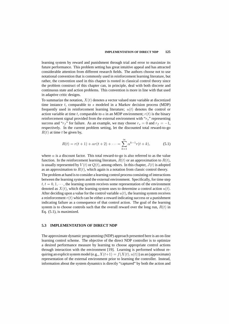
IMPLEMENTATION OF DIRECT NDP 125
learning system by reward and punishment through trial and error to maximize itsfuture performance. This problem setting has great intuitive appeal and has attractedconsiderable attention from different research fields. The authors choose not to usenotational convention that is commonly used in reinforcement learning literature, butrather, the convention used in this chapter is rooted in classical control theory sincethe problem construct of this chapter can, in principle, deal with both discrete andcontinuous state and action problems. This convention is more in line with that usedin adaptive critic designs.
To summarize the notation,X(t) denotes a vector valued state variable at discretizedtime instancet, comparable tos modeled in a Markov decision process (MDP)frequently used in reinforcement learning literature;u(t) denotes the control oraction variable at timet, comparable toa in an MDP environment;r(t) is the binaryreinforcement signal provided from the external environment with “rs” representingsuccess and “rf ” for failure. As an example, we may choosers = 0 andrf = −1,respectively. In the current problem setting, let the discounted total reward-to-goR(t) at timet be given by,
R(t) = r(t + 1) + αr(t + 2) + · · · =∞∑
k=1
αk−1r(t + k), (5.1)
whereα is a discount factor. This total reward-to-go is also referred to as the valuefunction. In the reinforcement learning literature,R(t) or an approximation toR(t),is usually represented byV (t) orQ(t), among others. In this chapter,J(t) is adoptedas an approximation toR(t), which again is a notation from classic control theory.
The problem at hand is to consider a learning control process consisting of interactionsbetween the learning system and the external environment. Specifically, for time stept, t = 0, 1, · · · , the learning system receives some representation of the environmentdenoted asX(t), which the learning system uses to determine a control actionu(t).After deciding upon a value for the control variableu(t), the learning system receivesa reinforcementr(t) which can be either a reward indicating success or a punishmentindicating failure as a consequence of that control action. The goal of the learningsystem is to choose controls such that the overall reward over the long run,R(t) inEq. (5.1), is maximized.
5.3 IMPLEMENTATION OF DIRECT NDP
The approximate dynamic programming (NDP) approach presented here is an on-linelearning control scheme. The objective of the direct NDP controller is to optimizea desired performance measure by learning to choose appropriate control actionsthrough interaction with the environment [19]. Learning is performed without re-quiring an explicit system model (e.g.,X(t+1) = f(X(t), u(t))) as an (approximate)representation of the external environment prior to learning the controller. Instead,information about the system dynamics is directly “captured” by both the action and

126 DIRECT NEURAL DYNAMIC PROGRAMMING
critic networks through learning. A general schematic diagram of the direct NDP isshown in Figure 5.1.
Action
Network
Critic
Network
System
R*
J(t)
J(t-1)
α
u(t)
X(t)
X(t)
r(t)
+
+
+
−
−
−
Fig. 5.1 Schematic diagram for implementation of direct neural dynamic programming.The solid lines denote system information flow, while the dashed lines represent error back-propagation paths to reduce the squared Bellman error:([r(t) + αJ(t)]− J(t− 1))2.
The direct NDP design structure in Figure 5.1 includes two networks, action andcritic, as building blocks. The critic network is trained toward optimizing a totalreward-to-go objective, namely to balance the Bellman equation. The action networkis trained such that the critic output approaches an ultimate objective of success,R∗ = rs
1−α , which is determined from Eq. (5.1). Due to this constraint a sufficientcondition for the applicability of the learning structure proposed in Figure 5.1 is thatα < 1 to ensure a convergent sequence to the ultimate performanceR∗ derived fromEq. (5.1). During the learning process, the action network is constrained by the criticto generate controls that optimize the future reward-to-go instead of only temporarilyoptimal solutions. In contrast to usual supervised neural network applications, thereare no readily available training sets of input-output pairs used for approximatingthe overall objective functionR(t) in terms of a least squares fit. Instead, both thecontrol actionu and the critic outputJ are updated according to an error functionthat changes from one time step to the next.
In the on-line learning control implementation, the controller is “naıve” when it startsto control. This is because, initially, both the action and critic networks possessrandom weights/parameters. Once a system state is observed, an action will besubsequently produced based on the parameters in the action network. A “better”control under the specific system state should result in a reduced Bellman error. Thisset of system operations will be reinforced through memory or association betweenstates and control output in the action network. Otherwise, the control will be adjustedthrough tuning the weights in the action network to minimize the Bellman error.

IMPLEMENTATION OF DIRECT NDP 127
5.3.1 The Critic Network
The critic network is used to provide an outputJ(t), which is an approximation forR(t), the weighted total future reward-to-go. The reward functionR(t) at timet isgiven by Eq. (5.1).
We define the prediction error, and consequently the Bellman error, for the criticelement as
ec(t) = [r(t) + αJ(t)]− J(t− 1), (5.2)
and the objective function to be minimized in the critic network is
Ec(t) =12e2c(t). (5.3)
Let wc denote the set of weight parameters in the critic network. The critic networkcan then be represented byJ = nnc(X,u, wc), wherennc denotes the critic network.The weight update rule for the critic network is a gradient-based adaptation given by
wc(t + 1) = wc(t) + ∆wc(t) (5.4)
∆wc(t) = lc(t)[−∂Ec(t)
∂wc(t)
](5.5)
∂Ec(t)∂wc(t)
=∂Ec(t)∂J(t)
∂J(t)∂wc(t)
(5.6)
wherelc(t) > 0 is the learning rate of the critic network at timet, which is typicallyselected to decrease with time to a small value. To re-iterate, the objective of thecritic network learning is to minimize the Bellman error by properly adjusting theweight parameters in the critic network.
5.3.2 The Action Network
The principle in adapting the action network is to back-propagate the error between thedesired ultimate performance objective, denoted byR∗, and the approximate functionJ from the critic network. Sincers has been defined as the reinforcement signal for“success,”R∗ is set to rs
1−α in the direct NDP design paradigm and in subsequent casestudies. In the action network, the state measurements are used as inputs to create acontrol as the output of the network. In turn, the action network can be implementedby either a linear or a nonlinear network, depending on the complexity of the problem.The weight update in the action network can be formulated as follows. Let
ea(t) = J(t)−R∗. (5.7)
Let wa denote the set of weight parameters in the action network, where the actionnetwork is represented byu = nna(X, wa). The weights in the action network are

128 DIRECT NEURAL DYNAMIC PROGRAMMING
updated to minimize the following performance error measure:
Ea(t) =12e2a(t). (5.8)
The update algorithm is then similar to the one in the critic network. By a gradientdescent rule
wa(t + 1) = wa(t) + ∆wa(t) (5.9)
∆wa(t) = la(t)[−∂Ea(t)
∂wa(t)
](5.10)
∂Ea(t)∂wa(t)
=∂Ea(t)∂J(t)
∂J(t)∂wa(t)
(5.11)
wherela(t) > 0 is the learning rate of the action network at timet, which usuallydecreases with time to a small value.
5.3.3 On-line Learning Algorithms
To provide readers with concrete implementation details, for the rest of this chapternonlinear multi-layer feed-forward networks are used as approximators for both theaction and the critic networks. Specifically, in this design, one hidden layer is usedin each network. As an example, and for the ease of introducing notation, a structurefor the nonlinear, multi-layer critic network is shown in Figure 5.2.
x2
u
xn
x1
wc(1)
J
wc(2)
Fig. 5.2 Schematic diagram for the implementation of a nonlinear critic network using afeed-forward network with one hidden layer.
In the critic network, the outputJ(t) is of the form,
J(t) =Nh∑
i=1
w(2)ci
(t)pi(t), (5.12)

IMPLEMENTATION OF DIRECT NDP 129
pi(t) =1− exp−qi(t)
1 + exp−qi(t), i = 1, · · · , Nh, (5.13)
qi(t) =n+1∑
j=1
w(1)cij
(t)xj(t), i = 1, · · · , Nh, (5.14)
whereqi is theith hidden node input of the critic network, andpi is the correspondingoutput of the hidden node.Nh is the total number of hidden nodes in the critic networkandn + 1 is the total number of inputs into the critic network including the analogaction valueu(t) from the action network. By applying the chain rule, the adaptationof the critic network is summarized below.
(1) ∆w(2)c (hidden to output layer):
∆w(2)ci
(t) = lc(t)
[− ∂Ec(t)
∂w(2)ci (t)
], (5.15)
∂Ec(t)
∂w(2)ci (t)
=∂Ec(t)∂J(t)
∂J(t)
∂w(2)ci (t)
= αec(t)pi(t). (5.16)
(2) ∆w(1)c (input to hidden layer):
∆w(1)cij
(t) = lc(t)
[− ∂Ec(t)
∂w(1)cij (t)
], (5.17)
∂Ec(t)
∂w(1)cij (t)
=∂Ec(t)∂J(t)
∂J(t)∂pi(t)
∂pi(t)∂qi(t)
∂qi(t)
∂w(1)cij (t)
(5.18)
= αec(t)w(2)ci
(t)[12
(1− p2
i (t))]
xj(t). (5.19)
The adaptation in the action network is implemented by a feed-forward networksimilar to the one in Figure 5.2 except that the inputs are then measured states and

130 DIRECT NEURAL DYNAMIC PROGRAMMING
the output is the actionu(t). The associated equations for the action network are,
u(t) =1− exp−v(t)
1 + exp−v(t), (5.20)
v(t) =Nh∑
i=1
w(2)ai
(t)gi(t), (5.21)
gi(t) =1− exp−hi(t)
1 + exp−hi(t), i = 1, · · · , Nh, (5.22)
hi(t) =n∑
j=1
w(1)aij
(t)xj(t), i = 1, · · · , Nh, (5.23)
wherev is the input to the action node, andgi andhi are the output and the inputof the hidden nodes of the action network, respectively. Since the only input to theaction network is the state measurements, there is no (n + 1)th term in (5.23) as inthe critic network (see Eq. (5.14) for comparison). The update rule for the nonlinearmulti-layer action network also contains two sets of equations.
(1) ∆w(2)a (hidden to output layer):
∆w(2)ai
(t) = la(t)
[− ∂Ea(t)
∂w(2)ai (t)
], (5.24)
∂Ea(t)
∂w(2)ai (t)
=∂Ea(t)∂J(t)
∂J(t)∂u(t)
∂u(t)∂v(t)
∂v(t)
∂w(2)ai (t)
, (5.25)
= ea(t)Nh∑
i=1
[w(2)
ci(t)
12
(1− p2
i (t))w(1)
ci,n+1(t)
].
[12
(1− u2(t)
)]gi(t)· (5.26)
In the above equations,∂J(t)∂u(t) is obtained by changing variables and by chain rule.
The result is the summation term. The termw(1)ci,n+1 is the weight associated with the
input element from the action network.
(2) ∆w(1)a (input to hidden layer):
∆w(1)aij
(t) = la(t)
[− ∂Ea(t)
∂w(1)aij (t)
], (5.27)
∂Ea(t)
∂w(1)aij (t)
=∂Ea(t)∂J(t)
∂J(t)∂u(t)
∂u(t)∂v(t)
∂v(t)∂gi(t)
∂gi(t)∂hi(t)
∂hi(t)
∂w(1)aij (t)
(5.28)
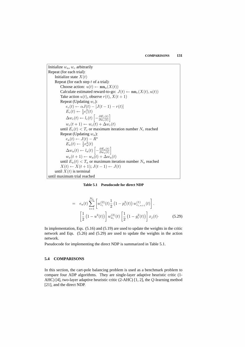
COMPARISONS 131
Initialize wa, wc arbitrarilyRepeat (for each trial):
Initialize stateX(t)Repeat (for each stept of a trial):
Choose action:u(t) ← nna(X(t))Calculate estimated reward-to-go:J(t) ← nnc(X(t), u(t))Take actionu(t), observer(t), X(t + 1)Repeat (Updatingwc):
ec(t) ← αJ(t)− [J(t− 1)− r(t)]Ec(t) ← 1
2e2c(t)
∆wc(t) ← lc(t)[−∂Ec(t)
∂wc(t)
]
wc(t + 1) ← wc(t) + ∆wc(t)until Ec(t) < Tc or maximum iteration numberNc reachedRepeat (Updatingwa):
ea(t) ← J(t)−R∗
Ea(t) ← 12e2
a(t)
∆wa(t) ← la(t)[−∂Ea(t)
∂wa(t)
]
wa(t + 1) ← wa(t) + ∆wa(t)until Ea(t) < Ta or maximum iteration numberNa reachedX(t) ← X(t + 1); J(t− 1) ← J(t)
until X(t) is terminaluntil maximum trial reached
Table 5.1 Pseudocode for direct NDP
= ea(t)Nh∑
i=1
[w(2)
ci(t)
12
(1− p2
i (t))w(1)
ci,n+1(t)
].
[12
(1− u2(t)
)]w(2)
ai(t)
[12
(1− g2
i (t))]
xj(t)· (5.29)
In implementation, Eqs. (5.16) and (5.19) are used to update the weights in the criticnetwork and Eqs. (5.26) and (5.29) are used to update the weights in the actionnetwork.
Pseudocode for implementing the direct NDP is summarized in Table 5.1.
5.4 COMPARISONS
In this section, the cart-pole balancing problem is used as a benchmark problem tocompare four ADP algorithms. They are single-layer adaptive heuristic critic (1-AHC) [4], two-layer adaptive heuristic critic (2-AHC) [1, 2], theQ-learning method[21], and the direct NDP.

132 DIRECT NEURAL DYNAMIC PROGRAMMING
The cart-pole balancing problem is a classic control problem used in early reinforce-ment learning literature [1, 2, 4]. It has since been adopted frequently as a benchmarkexample to evaluate various learning algorithms [12, 13].
The system model under consideration was identical to that in [4]. This modelprovided four state variables: 1)x(t), position of the cart on the track; 2)θ(t), angleof the pole with respect to the vertical position; 3)x(t), cart velocity; 4)θ(t), angularvelocity.
In this study a run consisted of a maximum of 50,000 consecutive trials. It wasconsidered successful if the last trial (trial number less than 50,000) of the run lasted600,000 time steps. Otherwise, if the controller was unable to learn to balance thecart-pole within 50,000 trials (i.e., none of the 50,000 trials lasted over 600,000time steps), then the run was considered unsuccessful. In simulations, we used 0.02seconds for each time step, and a trial was a complete process from start to fall.A pole was considered fallen when the pole was outside the range of[−12, 12]and/or the cart was beyond the range of[−2.4, 2.4] meters in reference to the centralposition on the track. Note that although the forceF applied to the cart was binary,the controlu(t) fed into the critic network as shown in Figure 5.1 was continuous.
The direct NDP was implemented following the steps given in Table 5.1. Note thatthe weights in the action and the critic networks were trained using their internalcycles,Na andNc, respectively. That is, within each time step the weights of thetwo networks were updated for at mostNa andNc times, respectively, or stoppedonce the internal training error thresholdTa andTc were met. The parametersNa,Nc, Ta, andTc were later collectively referred to as stopping criteria.
Learning system performance was compared to evaluate the learning controller’soverall ability to learn the task, to sustain noise, and to handle complex dynamics.
5.4.1 Algorithm Implementation
Here is a summary of implementation details of the four algorithms.
• Single-layer adaptive heuristic critic (1-AHC)
The 1-AHC is one of the earliest reinforcement learning methods [4]. Thelearning controller implemented was from the original C source code offRichard Sutton’s web site. The parameters were kept the same as follows:Action learning rate (α) = 1000; Critic learning rate (β) =0.5; TD discountfactor (γ) = 0.95; Decay rate (λ) = 0.8; E trace decay rate (δ) = 0.9. Quantizedstate variables were used as inputs. The state space was divided into 162regions. A 162-component binary valued vector was a representation of onestate input for the system. In this implementation, all components were zeroexcept for one corresponding to the region where the current state resided.
• Two-layer adaptive heuristic critic (2-AHC)
The 2-AHC is a direct extension of the 1-AHC by using two layer neuralnetworks to present the actor and critic units, respectively [1, 2]. Therefore,

COMPARISONS 133
continuous state inputs can be directly fed into each network after propernormalization. The algorithm implemented was from the original C sourcecode off Charles Anderson’s web site. The parameters were kept the same:Action learning rate (α) = 1.0; Hidden action learning rate (αh) =0.2; Criticlearning rate (β) = 0.2; Hidden critic learning rate (βh) = 0.05.
• Q-learning
The one-stepQ-learning withε-greedy was implemented as described in [21].The same input quantization as in 1-AHC was used forQ-learning. A Q-tablewith 162×2 entries were created and with initialQ values chosen to be 0. Theε-greedy policy allowed for an interleaving of “exploration” and “exploitation”.The learning parameters were chosen as follows: Q learning rate (β)= 0.5; TDdiscount factor (γ) = 0.999;ε = 1× 10⁻⁵.
• Direct NDP
The direct NDP was implemented per Table 5.1. The learning parameters wereas follows: lc(0)=0.3; la(0)=0.3; lc(f)=0.005;la(f)=0.005, wherelc(0) wasthe initial learning rate for the critic network which was later reduced tolc(f).The same can be said aboutla(0) and la(f). The stopping criteria used intraining the neural networks were:Nc=50;Na=100;Tc=0.05;Ta=0.005.
5.4.2 Simulation Implementation
All comparisons were based on 20 runs. A successful run was one where its last trialsustained 600,000 sequential control actions without failure (corresponding to 3hrand 20m in real time). Each implementation was written in C and ran on a PentiumIV PC.
Thefirst setof experiments (with results shown in Table 5.2, Table 5.3, and Table 5.4)was to compare learning performance in a noisy cart-pole system. For each of thefour algorithms, each run and each trial were conducted from the center start position.Three different noise levels (1%, 2%, and 5%) were evaluated. Uniform noise wasadded to the system states as follows. Letx be the current state variable. If thenoise level was 5%, then the actual state values that fed into the learning controllerwasx + random(−x ∗ 0.05, x ∗ 0.05). The same principle applied to other noiselevels. In addition to sensor noise, a very small random disturbance with a magnitudeless than±0.0001 was added into the system state measurements to ensure that thesimulated system was subject to some level of noise even atx = 0. To provide areference point, we also tabulated learning performance when no noise was added tothe system. Results were compared for 1) number of trials needed to complete thelearning control task; 2) learning time measured by CPU seconds; and 3) number offailed runs.
The second setof experiments (with results shown in Table 5.5) was to evaluatelearning performance as in Anderson [1, 2] where both the cart and the pole startedfrom random initial positions with random initial velocities. But no noise was added

134 DIRECT NEURAL DYNAMIC PROGRAMMING
in this study. At the start of every trial, the positions and the velocities were set tonew random values. Specifically, the four initial states were uniformly distributedwithin the following ranges:x ∈ [-2.4, 2.4]; x ∈ [-1.5, 1.5];θ ∈ [−12, 12]; θ ∈[-1.5, 1.5].
5.4.3 Simulation Results
Statistical results for the first set of experiments are summarized in Tables 5.2 - 5.4.The results shown in Table 5.2 for 1-AHC, 2-AHC andQ-learning with 0% noisecase were very close to those obtained in [12] when the authors compared the threealgorithms to their SANE algorithm, using the identical cart-pole balancing system.The simulation results for 1-AHC, 2-AHC andQ-learning for other cases in Table5.2 and Table 5.3 were comparable to the ones provided in the technical report [13].The actual numbers may be a little different since a longer simulation time and asmaller number of allowed trials in each run were used to obtain the results.
Mean TrialsNoise Level 1-AHC 2-AHC Q-learning Direct NDP
0% 320 5674 1815 10
1% 187 4890 3322 134
2% 2402 9887 9200 73
5% N/A 14145 N/A 110
Table 5.2 Comparison of learning system performance measured by trials needed tolearn the task under different levels of noise from “0” initial condition.
Failed RunsNoise Level 1-AHC 2-AHC Q-learning Direct NDP
0% & 1% 0 0 0 0
2% 0 1 0 0
5% 20 2 20 0
Table 5.3 Comparison of learning system performance measured by number of failedruns out of 20 under different levels of noise from “0” initial condition.
In obtaining the above results, it is noticed that direct NDP uses the least numberof trials. But, that does not imply the shortest CPU time. In addition,Q-learning
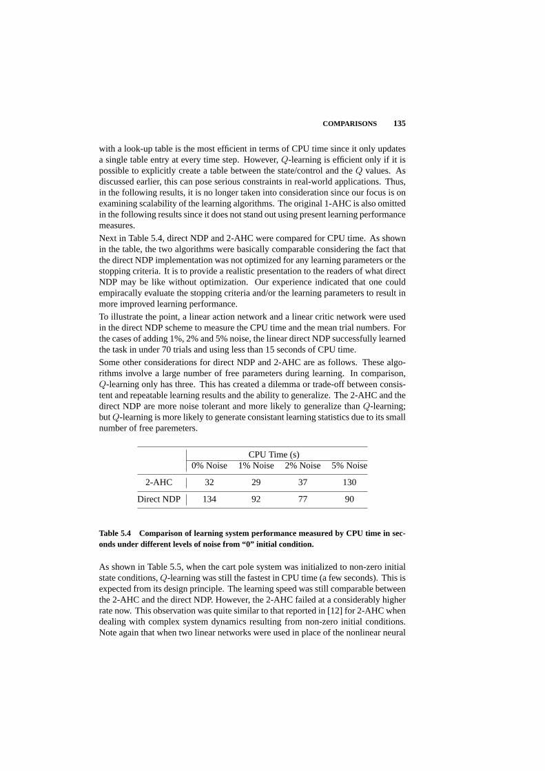
COMPARISONS 135
with a look-up table is the most efficient in terms of CPU time since it only updatesa single table entry at every time step. However,Q-learning is efficient only if it ispossible to explicitly create a table between the state/control and theQ values. Asdiscussed earlier, this can pose serious constraints in real-world applications. Thus,in the following results, it is no longer taken into consideration since our focus is onexamining scalability of the learning algorithms. The original 1-AHC is also omittedin the following results since it does not stand out using present learning performancemeasures.
Next in Table 5.4, direct NDP and 2-AHC were compared for CPU time. As shownin the table, the two algorithms were basically comparable considering the fact thatthe direct NDP implementation was not optimized for any learning parameters or thestopping criteria. It is to provide a realistic presentation to the readers of what directNDP may be like without optimization. Our experience indicated that one couldempiracally evaluate the stopping criteria and/or the learning parameters to result inmore improved learning performance.
To illustrate the point, a linear action network and a linear critic network were usedin the direct NDP scheme to measure the CPU time and the mean trial numbers. Forthe cases of adding 1%, 2% and 5% noise, the linear direct NDP successfully learnedthe task in under 70 trials and using less than 15 seconds of CPU time.
Some other considerations for direct NDP and 2-AHC are as follows. These algo-rithms involve a large number of free parameters during learning. In comparison,Q-learning only has three. This has created a dilemma or trade-off between consis-tent and repeatable learning results and the ability to generalize. The 2-AHC and thedirect NDP are more noise tolerant and more likely to generalize thanQ-learning;butQ-learning is more likely to generate consistant learning statistics due to its smallnumber of free paremeters.
CPU Time (s)0% Noise 1% Noise 2% Noise 5% Noise
2-AHC 32 29 37 130
Direct NDP 134 92 77 90
Table 5.4 Comparison of learning system performance measured by CPU time in sec-onds under different levels of noise from “0” initial condition.
As shown in Table 5.5, when the cart pole system was initialized to non-zero initialstate conditions,Q-learning was still the fastest in CPU time (a few seconds). This isexpected from its design principle. The learning speed was still comparable betweenthe 2-AHC and the direct NDP. However, the 2-AHC failed at a considerably higherrate now. This observation was quite similar to that reported in [12] for 2-AHC whendealing with complex system dynamics resulting from non-zero initial conditions.Note again that when two linear networks were used in place of the nonlinear neural

136 DIRECT NEURAL DYNAMIC PROGRAMMING
networks, direct NDP learned the task from non-zero initial conditions in under 90trials using less than 8 seconds of CPU time.
CPU Time (s) Mean Trials Failed Runs
1-AHC 162 2309 1
2-AHC 54 12310 10
Q-learning 4 1553 0
Direct NDP 41 64 0
Table 5.5 Comparison of learning system performance measured by CPU time, meantrials and failed runs for the pole balancing task starting from random initial conditionwithout noise.
5.5 A CONTINUOUS STATE CONTROL PROBLEM
The direct NDP design introduced in the previous sections was applied to a continuousstate on-line learning control problem. The triple-link inverted pendulum problemwith a single control input is illustrated in Figure 5.3.
5.5.1 Triple-link inverted pendulum with single control input
The system model for the triple-link problem was the same as that in [7]. The systemparameters used in this study were identical to those in [7] as well.
The only controlu (in volts) generated by the action network was converted intoforce by an analog amplifier through a conversion gainKs (in Newtons/volt). Insimulations,Ks = 24.7125 N/V. Each link could only rotate in the vertical planeabout the axis of a position sensor fixed to the top of each link.
There were eight state variables in this model: 1)x(t), position of the cart on thetrack; 2)θ1(t), vertical angle of the first link joint to the cart; 3)θ2(t), vertical angleof the second link joint to the first link; 4)θ3(t), vertical angle of the third link jointto the second link; 5)x(t), cart velocity; 6)θ1(t), angular velocity ofθ1(t); 7) θ2(t),angular velocity ofθ2(t); 8) θ3(t), angular velocity ofθ3(t).In the triple-link inverted pendulum problem, a run consisted of a maximum of 3,000consecutive trials. A run was considered successful if the last trial of the run lasted600,000 time steps. A unit time step was 5 ms. The constraints for the reinforcementlearning were: 1) the cart track extended 1.0m to both ends from the center position;2) the voltage applied to the motor was within [-30, 30]V range; 3) each link angleshould be within the range of[−20, 20] with respect to the vertical axis. In our

A CONTINUOUS STATE CONTROL PROBLEM 137
firstjoint
controlforce
x
θ1
θ2
θ3
L1
l1
mountjoint
secondjoint
Fig. 5.3 Illustration of the triple-link inverted pendulum problem with state and controlvariables defined as depicted.
simulations, condition 2 was assured by using a sigmoid function at the output of theaction node. For conditions 1) and 3), if either one failed or both failed, the systemprovided an indicative signalr = −1 at the moment of failure, otherwiser = 0 allthe time. Several experiments were conducted to evaluate the effectiveness of thedirect NDP design. The results are reported in the following.
5.5.2 Simulation results
Note that the triple-link system is highly unstable. To see this, observe that thepositive eigenvalues of the linearized system model are far away from zero (thelargest is around 10.0). In obtaining the linearized system model, the Coulombfriction coefficients are assumed to be negligible. Besides, the system dynamicschange fast. It requires a sampling time below 10 ms.
Since the analog output from the action network was directly fed into the system,the controller was more sensitive to actuator noise than when using a binary con-trol output. Experiments conducted included evaluations of direct NDP controllerperformance under uniform actuator noise, uniform or Gaussian sensor noise, andthe case without noise. Specifically, the actuator noise was implemented throughu(t) = u(t) + ρ, whereρ was a uniformly distributed random variable. For thesensor noise, both uniform and Gaussian random variables were added to the anglemeasurementsθ. The uniform state sensor noise was implemented throughθ = (1+noise percentage)× θ. Gaussian sensor noise was zero mean with variance of either0.1 or 0.2.

138 DIRECT NEURAL DYNAMIC PROGRAMMING
Before the presentation of our results, the learning parameters were summarized asfollows: lc(0)=0.8; lc(f)=0.001;la(0)=0.8; la(f)=0.001. The stopping criteria intraining the neural networks were:Nc=10;Na=200;Tc=0.01;Ta=0.001. Simulationresults are tabulated in Table 5.6.
Noise type success rate # of trials
None 97% 1194
Uniform 5% actuator 92% 1239
Uniform 10% actuator 84% 1852
Uniform 5% sensor onθ1 89% 1317
Uniform 10% sensor onθ1 80% 1712
Gaussian sensor onθ1 variance = 0.1 85% 1508
Gaussian sensor onθ1 variance = 0.2 76% 1993
Table 5.6 Performance evaluation of direct NDP learning controller when balancing atriple-link inverted pendulum. The second column represents the percentage of successfulruns out of 100. The third column depicts the average number of trials to learn the task.The average is taken over the successful runs.
Figure 5.4 is an example of typical angle trajectories of the triple-link under directNDP control for a successful learning trial.
The results presented in this case study have demonstrated the applicability of thedirect NDP designs to a non-trivial continuous state control problem. It is worthmentioning that the direct NDP controlled angle variations are significantly smallerthan those obtained from nonlinear control system design [7].
5.6 CALL ADMISSION CONTROL FOR CDMA CELLULARNETWORKS
In the present example, direct NDP was applied to call admission control in SIR-based power-controlled direct-sequence code-division multiple access (DS-CDMA)cellular networks, where SIR denotes signal-to-interference ratio. For a given setof parameters including traffic statistics and mobility characteristics, fixed call ad-mission control schemes can sometimes yield optimal solutions [16] using a gradeof service measure. However, such schemes are not adaptable to changing networkconditions [16, 9, 17, 18]. Therefore, we developed a direct NDP-based self-learningcall admission control algorithm for the CDMA wireless network application. Theperformance of the present algorithm was studied through computer simulations and

CALL ADMISSION CONTROL FOR CDMA CELLULAR NETWORKS 139
0 10 20 30 40 50 60 70 80 90 100−4
−2
0
2
4
Deg
rees
θ1
0 10 20 30 40 50 60 70 80 90 100−4
−2
0
2
4
Deg
rees
θ2
0 10 20 30 40 50 60 70 80 90 100−2
−1
0
1
2
Time Steps
Deg
rees
θ3
Fig. 5.4 Typical angle trajectories of the triple-link during a successful learning trial usingon-line NDP control when the system is free of noise.
compared with existing call admission control algorithms. Results show that the di-rect NDP-based self-learning call admission control algorithm outperforms existingcall admission control algorithms under the network conditions specified below.
Problem Definition
Consider a base station withN concurrent active connections. The power receivedfrom each connection is denoted bySn, n = 1, · · · , N . In an SIR-based power-controlled DS-CDMA network [18, 3, 6, 10], the desired value of the power levelSn
is a function of the number of active connections in the home cell (home base station)and total other cell interference. A DS-CDMA cellular network with a single classof service (e.g., voice) is considered. The maximum received power at a base stationfor that class of service is denoted byH.
Two types of calls, new and handoff, are considered for admission controls. Foran arriving call requesting admission, one of the two control actions, accept orreject, is selected. Typically handoff calls are given higher priority than new calls[16, 9, 17, 18]. This is accomplished by using different thresholds for new calls andhandoff calls as shown below.

140 DIRECT NEURAL DYNAMIC PROGRAMMING
The criteria for accepting new calls can be expressed as
u(t) =
1 (accept): if 0 < Snew ≤ T and0 < Sn ≤ H for n = 1, 2, · · · , N,
-1 (reject): else,
whereT ≤ H is the threshold for new calls.
For handoff calls, a more relaxed threshold is given as
u(t) =
1 (accept): if 0 < Shandoff ≤ H and0 < Sn ≤ H for n = 1, 2, · · · , N,
-1 (reject): else.
The objective of this study is to optimize the grade of service (GoS) measure undervarious, possibly changing environmental conditions and user behaviors. The GoSmeasure [28] is defined as
GoS = P (call blocking) + w × P (handoff failure), (5.30)
where the first term is the probability of call blocking and the second term is theprobability of handoff blocking with the weighting factorw (typically chosen as 10)signifying a relative emphasis on the two terms.
Algorithm Implementation
Since only binary control, accept or reject, was needed in call admission, only thecritic network shown in Figure 5.1 was utilized where the control input to the criticnetwork wasu(t) = +1 for accept andu(t) = −1 for reject. A correct admissiondecision was associated with a reward signal of “0” otherwise a penalty signal of apositive value. The inputs to the critic network were the system states, the admissioncontrol (accept or reject) and the call type (new call or handoff call). The systemstate was the total interference received at the base station. In DS-CDMA cellularsystems, interference increases as traffic load increases.
To formulate a proper value function for the learning controller, a cost is first associ-ated with each active connectionn as follows:
• for new call
En =
ξ ·max[
SnT − 1
], 0
, when u(t) = 1,
ξ ·max[
1− SnH
], 0
, when u(t) = −1,
(5.31)
• for handoff call
En = ξ ·max
u(t) ·[Sn
H− 1
], 0
, (5.32)

CALL ADMISSION CONTROL FOR CDMA CELLULAR NETWORKS 141
whereξ > 0 is a coefficient,T ≤ H, andEn ≥ 0 for all n = 1, · · · , N .
A collective cost is then chosen from allN connections as
E =
max0≤n≤N
(En), if u(t) = 1,
min0≤n≤N
(En), if u(t) = −1.(5.33)
We can now define an instantaneous reinforcement signalr as
r =E
1 + E. (5.34)
The instantaneous reinforcement signalr defined in (5.34) has the following prop-erties: (1)r ≈ 0 whenE << 1, and (2)r ≈ 1 whenE >> 1. The choice ofthe present reinforcement signal in (5.34) clearly shows minimum points (the flatareas) that our call admission control tries to reach and the points with high penaltyto avoid. The objective of the learning controller is to make the correct admissioncontrol decisions such that the total reward-to-goR(t) in Eq. (5.1) is optimized.We have thus formulated an approximate dynamic programming problem. Next, weuse the learning architecture shown in Figure 5.1 to obtain an approximate solution.Note again that in this example, the action network is omitted since the binary controldecision is well defined.
With the reinforcement signal given by (5.33) and (5.34), we have
0 < J(t) <1
1− α,
whereα is the discount factor in Eq. (5.1).
Alternatively, a different cost and consequently instantaneous reinforcement can bedefined in place of (5.31) as follows:
En =
ξ ·max[
SnH − 1
], 0
, when u(t) = 1, na ≤ Nh
ξ ·max[
SnT − 1
], 0
, when u(t) = 1, na > Nh
ξ ·max[
1− SnH
], 0
, when u(t) = −1
(5.35)
wherena is the number of handoff calls in the cell that are accepted and are stillactive, andNh is a fixed parameter indicating the threshold for low traffic load. It isexpected that different cost measure will lead to different system performance.
Data is collected prior to training the learning controller. When a call arrives, one canaccept or reject the call with any scheme and calculate the instantaneous reinforcementsignalr for the system as presented above. For instance, a call can be accepted andrejected simply by using a equal probability of 0.5. In the mean time, state andenvironmental data are collected corresponding to each action. These include total
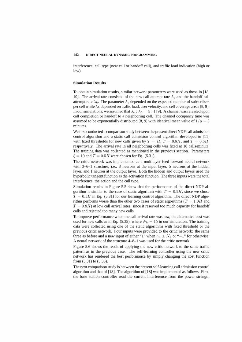
142 DIRECT NEURAL DYNAMIC PROGRAMMING
interference, call type (new call or handoff call), and traffic load indication (high orlow).
Simulation Results
To obtain simulation results, similar network parameters were used as those in [18,10]. The arrival rate consisted of the new call attempt rateλc and the handoff callattempt rateλh. The parameterλc depended on the expected number of subscribersper cell whileλh depended on traffic load, user velocity, and cell coverage areas [8, 9].In our simulations, we assumed thatλc : λh = 5 : 1 [9]. A channel was released uponcall completion or handoff to a neighboring cell. The channel occupancy time wasassumed to be exponentially distributed [8, 9] with identical mean value of1/µ = 3minutes.
We first conducted a comparison study between the present direct NDP call admissioncontrol algorithm and a static call admission control algorithm developed in [11]with fixed thresholds for new calls given byT = H, T = 0.8H, andT = 0.5H,respectively. The arrival rate in all neighboring cells was fixed at 18 calls/minute.The training data was collected as mentioned in the previous section. Parametersξ = 10 andT = 0.5H were chosen for Eq. (5.31).
The critic network was implemented as a multilayer feed-forward neural networkwith 3–6–1 structure, i.e., 3 neurons at the input layer, 5 neurons at the hiddenlayer, and 1 neuron at the output layer. Both the hidden and output layers used thehyperbolic tangent function as the activation function. The three inputs were the totalinterference, the action and the call type.
Simulation results in Figure 5.5 show that the performance of the direct NDP al-gorithm is similar to the case of static algorithm withT = 0.5H, since we choseT = 0.5H in Eq. (5.31) for our learning control algorithm. The direct NDP algo-rithm performs worse than the other two cases of static algorithms (T = 1.0H andT = 0.8H) at low call arrival rates, since it reserved too much capacity for handoffcalls and rejected too many new calls.
To improve performance when the call arrival rate was low, the alternative cost wasused for new calls as in Eq. (5.35), whereNh = 15 in our simulation. The trainingdata were collected using one of the static algorithms with fixed threshold or theprevious critic network. Four inputs were provided to the critic network: the samethree as before and a new input of either “1” whenna ≤ Nh or “−1” for otherwise.A neural network of the structure 4–8–1 was used for the critic network.
Figure 5.6 shows the result of applying the new critic network to the same trafficpattern as in the previous case. The self-learning controller using the new criticnetwork has rendered the best performance by simply changing the cost functionfrom (5.31) to (5.35).
The next comparison study is between the present self-learning call admission controlalgorithm and that of [18]. The algorithm of [18] was implemented as follows. First,the base station controller read the current interference from the power strength

CALL ADMISSION CONTROL FOR CDMA CELLULAR NETWORKS 143
10 15 20 25 30 3510
−4
10−3
10−2
10−1
100
101
GoS
Call arrival rate in the center cell (calls/minute)
Call arrival rate in neighboring cells: 18 calls/minute
self−learningT=H T=0.8H T=0.5H
Fig. 5.5 Comparison result using cost function defined in (5.31).
10 15 20 25 30 3510
−4
10−3
10−2
10−1
100
101
GoS
Call arrival rate in the center cell (calls/minute)
Call arrival rate in neighboring cells: 18 calls/minute
self−learningT=H T=0.8H T=0.5H
Fig. 5.6 Comparison study using cost function defined in (5.35).
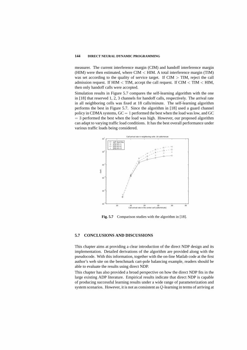
144 DIRECT NEURAL DYNAMIC PROGRAMMING
measurer. The current interference margin (CIM) and handoff interference margin(HIM) were then estimated, where CIM< HIM. A total interference margin (TIM)was set according to the quality of service target. If CIM> TIM, reject the calladmission request. If HIM< TIM, accept the call request. If CIM< TIM < HIM,then only handoff calls were accepted.
Simulation results in Figure 5.7 compares the self-learning algorithm with the onein [18] that reserved 1, 2, 3 channels for handoff calls, respectively. The arrival ratein all neighboring cells was fixed at 18 calls/minute. The self-learning algorithmperforms the best in Figure 5.7. Since the algorithm in [18] used a guard channelpolicy in CDMA systems, GC= 1 performed the best when the load was low, and GC= 3 performed the best when the load was high. However, our proposed algorithmcan adapt to varying traffic load conditions. It has the best overall performance undervarious traffic loads being considered.
10 15 20 25 30 3510
−4
10−3
10−2
10−1
100
101
GoS
Call arrival rate in the center cell (calls/minute)
Call arrival rate in neighboring cells: 18 calls/minute
self−learning[25] GC=1 [25] GC=2 [25] GC=3
Fig. 5.7 Comparison studies with the algorithm in [18].
5.7 CONCLUSIONS AND DISCUSSIONS
This chapter aims at providing a clear introduction of the direct NDP design and itsimplementation. Detailed derivations of the algorithm are provided along with thepseudocode. With this information, together with the on-line Matlab code at the firstauthor’s web site on the benchmark cart-pole balancing example, readers should beable to evaluate the results using direct NDP.
This chapter has also provided a broad perspective on how the direct NDP fits in thelarge existing ADP literature. Empirical results indicate that direct NDP is capableof producing successful learning results under a wide range of parameterization andsystem scenarios. However, it is not as consistent asQ-learning in terms of arriving at
CONCLUSIONS AND DISCUSSIONS 145
similar controllers after learning.Q-learning has very few free parameters, which isthe key to producing consistent learning results or solutions. However, as discussedearlier in the chapter, it is difficult to scale or generalize for large problems.
As an alternative to a tabulated value function for each possible state and controlaction, a neural network based value function approximation has the advantage ofgeneralization over the input space and being more resistant to noise. However atrade-off, observed empirically, is that on-line training of the neural value functionmay not always be accurate when compared to table-based approaches. This ismainly due to the randomness in parameter initialization, and the possibility that theparameter set converges to a local minimum in the error function space. With thissaid, our experience indicate that direct NDP is in general insensitive to parameterssuch as initial weights in the action and/or critic network and the learning ratecoefficients as long as they satisfy some general guidelines such as those specified instochastic approximation. Simulation results in the present chapter and Chapter 21have demonstrated that the direct NDP mechanism is capable of handling complexsystem dynamics, and it is robust in the presence of noise and disturbance.
The examples used in this chapter are continuous state problems. The triple-linkpendulum is a multi-state-single-control problem. Even though still a toy problem, itis not an easy problem for a typical classic controller. The three controlled pendulumangles shown in Figure 5.4 are much tighter than those in [7]. Later in Chapter21, direct NDP is used to control a helicopter under realistic flying conditions forstabilization, maneuvering, and reconfiguration after some component failure. Allthese results point to the possibility that direct NDP type of designs do have thepotential to generalize. However many challenges remain to be addressed.
Direct NDP is a model-independent approach to ADP. As seen from comparisons toQ-learning and actor-critic methods, even though clearly defined gradient informationmay have provided a clear parameter search direction, it still contains certain levelsof randomness due to the very nature of neural networks as approximators. Arecent study has demonstrated that this randomness can result in large variancesin controller bandwidth and other control performance measures [27]. This is notsurprising since unlike many classic control design methods where specific systemperformance measures are explicitly taken into design consideration, in the ADPsetting, one is only given a delayed, qualitative measure of the systems’ well being.The immediate issue is whether or not one can take advantage of a system model anda priori system knowledge and use them in the design process.
As discussed earlier, a good learning controller should be one that learns to perform atask quickly and also with a guarantee to learn to perform the task successfully throughtrial and error. Another factor that may not be explicitly present in the reinforcementsignal is the degree of meeting the performance requirement. In both pendulum casestudies, however, it is quite intriguing to see that the learning controllers not onlybalanced the poles, but also maintained the poles as centered as possible.
In summary, our results have demonstrated the potential of direct NDP in solvinglarge scale problems guided by delayed, high-level feedbacks despite the open issuesdiscussed earlier.

146 DIRECT NEURAL DYNAMIC PROGRAMMING
Acknowledgments
The first and second authors’ research was supported by the National Science Foundationunder grants ECS-0002098 and ECS-0233529. The third author’s research was supported bythe National Science Foundation under grants ECS-9996428 and ANI-0203063.

Bibliography
1. C. Anderson, “Strategy learning with multi-layer connectionist representa-tions,” Proceedings of the Fourth International Workshop on Machine Learning,pp. 103-114, 1987.
2. C. Anderson, “Learning to control an inverted pendulum using neural networks,”IEEE Control Systems Magazine,vol. 9, no. 3, pp. 31-37, 1989.
3. S. Ariyavisitakul, “Signal and interference statistics of a CDMA system withfeedback power control - Part II,”IEEE Transactions on Communications,vol. 42, pp. 597-605, 1994.
4. A. G. Barto, R. S. Sutton, and C. W. Anderson, “Neuron like adaptive ele-ments that can solve difficult learning control problems,”IEEE Transactions OnSystems, Man, and Cybernetics, vol. 13, pp. 834-847, 1983.
5. D. P. Bertsekas, and J. N. Tsitsiklis,Neuro-Dynamic Programming,AthenaScientific, 1996.
6. Z. Dziong, M. Jia, and P. Mermelstein, “Adaptive traffic admission for integratedservices in CDMA wireless-access networks,”IEEE Journal on Selected Areasin Communications,vol. 14, pp. 1737-1747, 1996.
7. K. D. Eltohamy, and C. Y. Kuo, “Nonlinear optimal control of a triple linkinverted pendulum with single control input,”International Journal of Control,vol. 69, no. 2, pp. 239-256, 1998.
8. R. A. Guerin, “Channel occupancy time distribution in a cellular radio system,”IEEE Transactions on Vehicular Technology,vol. 35, pp. 89-99, 1987.
9. D. Hong, and S. S. Rappaport, “Traffic model and performance analysis for cel-lular mobile radio telephone systems with prioritized and nonprioritized handoffprocedures,”IEEE Transactions on Vehicular Technology,vol. 35, pp. 77-92,1986.
10. D. K. Kim, and D. K. Sung, “Capacity estimation for an SIR-based power-controlled CDMA system supporting ON-OFF traffic,”IEEE Transactions onVehicular Technology,vol. 49, pp. 1094-1100, 2000.
147

148 BIBLIOGRAPHY
11. D. Liu, and Y. Zhang, “An adaptive call admission control algorithm for SIR-based power-controlled integrated services CDMA cellular networks,”Proceed-ings of the International Conference on Telecommunications,pp. 610-638, 2002.
12. D. E. Moriarty, and R. Miikkulainen, “Efficient reinforcement learning throughsymbiotic evolution,”Machine Learning,vol. 22, no. 11-32, pp. 11-32, 1996.
13. M. Pendrith, “On reinforcement learning of control actions in noisy and non-markovian domains,”Technical Report UNSW-CSE-TR-9410,1994.
14. D. V. Prokhorov, R. A. Santiago, and D. C. Wunsch II, “Adaptive critic designs:a case study for neuro-control,”Neural Networks,vol. 8, pp. 1367-1372, 1995.
15. D. V. Prokhorov, and D. C. Wunsch II, “Adaptive critic designs,”IEEE Transac-tions on Neural Networks,vol. 8, no. 5, pp. 997-1007, 1997.
16. R. Ramjee, D. Towsley, and R. Nagarajan, “On optimal call admission controlin cellular networks,”Wireless Networks,vol. 3, no. 1, pp. 29-41, 1997.
17. S. S. Rappaport, and C. Purzynski, “Prioritized resource assignment for mobilecellular communication systems with mixed services and platform types,”IEEETransactions on Vehicular Technology,vol. 45, pp. 443-458, 1996.
18. S. M. Shin, C.-H. Cho, and D. K. Sung, “Interference-based channel assignmentfor DS-CDMA cellular systems,”IEEE Transactions on Vehicular Technology,vol. 48, pp. 233-239, 1999.
19. J. Si, and Y. Wang, “Online learning control by association and reinforcement,”IEEE Transactions on Neural Networks,vol. 12, no. 2, pp. 264-276, 2001.
20. R. S. Sutton, and A. G. Barto,Reinforcement Learning: An Introduction,TheMIT Press, 1998.
21. C. J. C. H. Watkins,Learning from Delayed Rewards,Ph.D. Dissertation, Uni-versity of Cambridge, 1989.
22. P. Werbos, “Advanced forecasting methods for global crisis warning and modelsof intelligence,”General System Yearbook,vol. 22, pp. 25-38, 1977.
23. P. Werbos, “A menu of design for reinforcement learning over time,”NeuralNetworks for Control,in W. T. Miller III, R. S. Sutton, & P. J. Werbos (Eds.),MIT Press, 1990.
24. P. Werbos, “Neuro-control and supervised learning: An overview and valuation,”Handbook of Intelligent Control,in D. White, & D. Sofge (Eds.), Van NostrandReinhold, 1992.
25. Werbos, P., “Approximate dynamic programming for real-time control and neuralmodeling,” Handbook of Intelligent Control,in D. White, & D. Sofge (Eds.),Van Nostrand Reinhold, 1992.

BIBLIOGRAPHY 149
26. P. Werbos, “Tutorial on neurocontrol, control theory and related techniques:from back propagation to brain-like intelligent systems,”12th Intl Conferenceon Math. & Computer Modeling & Scientific Computing,1999. Also availableat www.iamcm.org/pwerbos/.
27. L. Yang, J. Si, K. Tsakalis, and A. Rodriguez, “Analyzing and enhancing directNDP designs using a control-theoretic approach,”IEEE International Symposiumon Intelligent Control,pp. 529-532, 2003.
28. “A guide to DECT features that influence the traffic capacity and the maintenanceof high radio link transmission quality, including the results of simulations,”ETSITechnical Report: ETR 042,1992.

6 The Linear ProgrammingApproachto Approximate DynamicProgramming
DANIELA PUCCI DE FARIAS
Massachusetts Institute of Technology
Editor’s Summary: This chapter addresses the issue of the “curse of dimensional-ity” by treating ADP as the “dual” of the linear programming problem and introducesthe concept of approximate linear programming (ALP). It provides a brief introduc-tion to the use of Markov Decision Process models. For a more comprehensive studyof MDP models, and the techniques that can be used with them, read Chapters 11and 12. This chapter discusses the performance of approximate LP policies, approx-imation error bounds, and provides an application to queuing networks. Anotherqueuing network example can be found in Chapter 12. The chapter finishes with anefficient constraint sampling scheme.
6.1 INTRODUCTION
Dynamic programming offers a unified approach to solving problems of stochasticcontrol. Central to the methodology is the cost-to-go function, which is obtained viasolving Bellman’s equation. The domain of the cost-to-go function is the state spaceof the system to be controlled, and dynamic programming algorithms compute andstore a table consisting of one cost-to-go value per state. Unfortunately, the size ofa state space typically grows exponentially in the number of state variables. Knownas thecurse of dimensionality, this phenomenon renders dynamic programmingintractable in the face of problems of practical scale.
One approach to dealing with the curse of dimensionality is to generate an ap-proximation within a parameterized class of functions, in a spirit similar to that ofstatistical regression. In particular, to approximate a cost-to-go functionJ∗ map-
150

INTRODUCTION 151
ping a state spaceS to reals, one would design a parameterized class of functionsJ : S×<K 7→ <, and then compute a parameter vectorr ∈ <K to “fit” the cost-to-gofunction, so that
J(·, r) ≈ J∗.
Note that there are two important preconditions to the development of an effectiveapproximation. First, it is necessary to choose a parameterizationJ that can closelyapproximate the desired cost-to-go function, i.e., the parameterization must be suchthat infr ‖J∗ − J(·, r)‖ is small. Second, it is necessary to have an algorithm thatidentifies a parameter vectorr such that‖J∗ − J(·, r)‖ is small.
At this stage, choosing appropriate classes of parametric functions is an art. Onemust balance issues such as efficiency of computation and storage ofh, difficulty incomputing appropriate parametersr, and ability of the parametric class to produce rea-sonable approximations. In practice, the choice of a suitable class typically requiresanalysis and/or experimentation with the specific problem at hand. “Regularities”associated with the function, for example, can guide the choice of representation.
In this chapter, we assume that a linearly parameterized classJ is given. Such a classcan be represented by
J(·, r) =K∑
k=1
rkφk,
where eachφk is a “basis function” mappingS to < and the parametersr1, . . . , rK
represent basis function weights. We consider the problem of generating an appropri-ate parameterr throughapproximate linear programming(ALP) [25, 8], an algorithmbased on a formulation that generalizes the linear programming approach to exactdynamic programming [5, 11, 12, 13, 18, 20]. The development in this chapter istwofold. First, we analyze the performance of approximate linear programming. Weaddress questions such as:
• If the set of basis functions has the potential to produce a close approximationto the cost-to-go function, is approximate linear programming also able toproduce a close approximation?
• What guarantees can we offer for the expected costs induced by policies pro-duced by approximate linear programming? How close are they to the optimalcosts?
• How do the approximation errors and performance losses scale as we increasethe size of the state space of the system? What about increasing the dimensionof the state space?
Second, we develop some analysis leading to streamlined guidelines for implementa-tion of approximate linear programming. We investigate issues such as how differentchoices for the algorithm’s free parameters affect the quality of the approximationbeing generated, and how we can deal with the large number of constraints involvedin the linear programs that have to be solved by the algorithm.

152 THE LINEAR PROGRAMMING APPROACH TO ADP
6.1.1 Performance analysis for approximate linear programming
Over the years, interest in approximate dynamic programming has been fuelled toa large extent by stories of empirical success in applications such as backgammon[26], job shop scheduling [31], elevator scheduling [6] and pricing of Americanoptions [19, 29]. These case studies point to approximate dynamic programming as apotentially powerful tool for large-scale stochastic control. However, significant trialand error is involved in most success stories found in the literature, and duplicationof the same success in other applications has proven difficult. This is partly dueto a relatively poor understanding of how, why and when approximate dynamicprogramming algorithms work, and poses a barrier to the use of such algorithms inindustry. Hence the analysis of performance and errors associated with approximatedynamic programming algorithms is not only an interesting theoretical challenge butalso a practical necessity, and the recent advancements in the theoretical analysis ofapproximate linear programming can be viewed as steps toward the ultimate goalof developing approximate dynamic programming into a truly practical, streamlinedmethodology for aiding decision-making in large-scale problems.
The version of approximate linear programming described here was first introducedin [8] and represents a variant of the algorithm originally proposed by Schweitzer andSeidman [25]. While the original ALP algorithm may exhibit poor scaling properties,the version introduced in [8] enjoys strong theoretical guarantees.
A central question about any approximate dynamic programming algorithm is howwell it approximates the cost-to-go function. The quality of the approximationdepends on the choice of basis functions, hence the error induced by an approximatedynamic programming algorithm is usually characterized in relative terms — wecompare it against the best error that can be achieved given the selection of basisfunctions.
Section 6.5 presents an error bound establishing that approximate linear programmingyields an approximation error that is comparable to the best that can be achieved giventhe selection of basis functions. Besides offering guarantees about the behavior ofthe algorithm, the bound provides insight about the impact of the algorithm’s freeparameters onto the final approximation, thus leading to some guidance in theirselection. It also provides information about how well the algorithm scales as theproblem dimensions increase.
Comparison of approximations to the cost-to-go function involve the choice of ametric on the space of functions over the state space that determines how gooddifferent approximations are perceived to be. Of course, the ultimate comparisonis the expected cost of the policy induced by the approximation, and this should bereflected in the metric being chosen. Section 6.4 includes a bound on the expectedcost increase due to using policies generated by approximate linear programminginstead of the optimal policy. The bound suggests a natural metric for comparisonof different approximations to the cost-to-go function and gives reassurance that theapproximation error bounds under consideration are meaningful, as they are stated interms of a metric that is compatible with the natural performance-based metric. The
INTRODUCTION 153
performance bound also provides guidance on how to set the free parameters in theapproximate linear programming algorithm so as to indirectly optimize performanceof the policy being obtained.
6.1.2 Constraint sampling
The approximate linear programming method, as the name suggests, relies on a linearprogram — theapproximate LP— to compute an approximation to the cost-to-gofunction. The number of variables involved in the approximate LP is relatively small— one per basis function. However, the number of constraints — one per state-actionpair — is generally intractable, and this presents an obstacle.
Section 6.7 describes an approximation scheme based on constraint sampling thatreplaces the approximate LP with an auxiliary linear program — thereduced LP— with the same variables and objective as the approximate LP, but with only asampled subset of constraints. The reduced LP is motivated by the fact that, becausethere is a relatively small number of variables in the approximate LP, many of theconstraints should have a minor impact on the feasible region and do not need to beconsidered; in particular, it can be shown that, by sampling a tractable number ofconstraints according to any given distribution, the solution of the resulting reducedLP is guaranteed to benear-feasiblewith high probability. In other words, with highprobability, the set of constraints violated by the solution of the reduced LP has smallprobability under the sampling distribution.
The fact that constraint sampling yields near-feasible solutions is a general propertyof LP’s with a large number of constraints and relatively few variables. Propertiesspecific to approximate linear programming imply that, under certain conditions, theerror in approximating the cost-to-go function yielded by the reduced LP should beclose to that yielded by the approximate LP, with high probability.
6.1.3 Literature review
Much of the effort in the literature on approximate linear programming has been di-rected toward efficient implementation of the algorithm. Some general analysis of thealgorithm can be found in [27, 28, 15]. Trick and Zin [27, 28] develop heuristics forcombining the linear programming approach with successive state aggregation/gridrefinement in two-dimensional problems. Some of their grid generation techniquesare based on stationary state distributions, which also appear in the analysis of state-relevance weights presented here. An important feature of the linear programmingapproach is that it generateslower boundsas approximations to the cost-to-go func-tion; Gordon [15] discusses problems that may arise from this fact and suggestsconstraint relaxation heuristics. One of these problems is that the linear programused in the approximate linear programming algorithm may be overly constrained,which may lead to poor approximations or even infeasibility. The approach takenhere prevents this — part of the different between the variant of approximate linearprogramming presented here and the original one proposed by Schweitzer and Seid-
154 THE LINEAR PROGRAMMING APPROACH TO ADP
mann is that the former involves certain basis functions that guarantee feasibility andalso lead to guaranteed bounds on the approximation error.
The constraint sampling scheme presented here does not exploit any possible reg-ularity associated with structure in the constraints arising in specific problems, ora particular choice of basis functions, which might lead to much tighter bounds oreven methods for exact solution of the approximate LP. Results of this nature can befound in the literature. Morrison and Kumar [21] formulate approximate linear pro-gramming algorithms for queueing problems with a certain choice of basis functionsthat renders all but a relatively small number of constraints redundant. Guestrin etal. [17] exploit the structure arising when factored linear architectures are used forapproximating the cost-to-go function in factored MDP’s to efficiently implementapproximate linear programming with a tractable number of constraints. Traditionalmethods designed to deal with linear programs with large numbers of constraints,such as cutting planes and column generation, may also be useful in specific settings.Schuurmans and Patrascu [24] devise a constraint generation scheme for factoredMDP’s with factored linear architectures that lacks the guarantees of the algorithmpresented in [17], but requires a smaller amount of time on average. Grotschel [16]presents an efficient cutting-plane method for the traveling salesman problem.
Approximate linear programming also appears in the literature as a tool for analysisand solution of stochastic control problems in various application areas. Paschalidisand Tsitsiklis [22] apply the algorithm to two-dimensional problems arising in pricingof network services. Morrison and Kumar [21] use approximate linear programmingto derive bounds on the performance of queueing networks. Adelman [1, 2] usesapproximate linear programming as an analytical tool aiding in the development ofpolicies for inventory control. de Farias et al. [7] use approximate linear programmingto derive policies for optimal resource allocation in web server farms.
The results presented here appeared originally in articles [8, 9] by de Farias and VanRoy. Proofs are omitted and can be found in these references.
6.1.4 Chapter organization
This chapter is organized as follows. Sections 6.2 and 6.3 provide some background,including a formulation of the stochastic control problem under consideration anddiscussion of linear programming approaches to exact and approximate dynamicprogramming. Section 6.4 presents bounds on the performance of policies generatedby ALP, and a discussion on how performance optimization can be incorporatedin the algorithm by appropriate choice of certain parameters in the approximateLP. Section 6.5 presents bounds on the error in the approximation to the cost-to-gofunction yielded by ALP. The error bounds involve problem-dependent terms, andSection 6.6 focuses on characteristics of these terms in examples involving queueingnetworks. Section 6.7 describes a constraint sampling scheme for dealing with thelarge number of constraints involved in the approximate LP. Finally, Section 6.8discusses directions for future research on approximate linear programming.

MARKOV DECISION PROCESSES 155
6.2 MARKOV DECISION PROCESSES
A Markov decision process (MDP) in discrete-time is characterized by a tuple(S,A·, P·(·, ·), g·(·)), with the following interpretation.S represents a finite statespaceS of cardinality|S| = N . For each statex ∈ S, there is a finite set of availableactionsAx. Taking actiona ∈ Ax when the current state isx incurs costga(x).State transition probabilitiesPa(x, y) represent, for each pair(x, y) of states andeach actiona ∈ Ax, the probability that the next state will bey given that the currentstate isx and the current action isa.
A policy u is a mapping from states to actions. Given a policyu, the dynamics ofthe system follow a Markov chain with transition probabilitiesPu(x)(x, y). For eachpolicy u, we define a transition matrixPu whose(x, y)th entry isPu(x)(x, y).We letxt, t = 0, 1, . . . denote the state of the MDP at timet.
The problem of stochastic control amounts to selection of a policy that optimizesa given criterion. We will employ as the optimality criterion the infinite-horizondiscounted cost
Ju(x) = E
[ ∞∑t=0
αtgu(xt)|x0 = x
], (6.1)
wheregu(x) is used as shorthand forgu(x)(x) and the discount factorα ∈ (0, 1)reflects inter–temporal preferences. Throughout the paper, we letE[·] denote expectedvalue. It is well known that there exists a single policyu that minimizesJu(x)simultaneously for allx, and the goal is to identify that policy.
Let us define operatorsTu andT by
TuJ = gu + αPuJ
andTJ = min
uTuJ,
where the minimization is carried out component–wise. For any vectorJ , we alsodefine thegreedypolicy associated withJ given by
uJ(x) = argmina∈Ax
(ga(x) + α∑
y∈SPa(x, y)J(y)).
Dynamic programming involves solution of Bellman’s equation
J = TJ.
The unique solutionJ∗ of this equation is the optimal cost–to–go function
J∗ = minu
Ju,
and a policy is optimal if and only if it is greedy with respect toJ∗.

156 THE LINEAR PROGRAMMING APPROACH TO ADP
Dynamic programming offers a number of approaches to solving Bellman’s equation.One of particular relevance to our chapter makes use of linear programming, as wewill now discuss. Consider the problem
maxJ cT J (6.2)
s.t. TJ ≥ J,
wherec : S 7→ < is a vector with positive components, which we will refer to asstate–relevance weights, andcT denotes the transpose ofc. It can be shown that anyfeasibleJ satisfiesJ ≤ J∗. It follows that, for any set of positive weightsc, J∗ isthe unique solution to (6.2).
Note thatT is a nonlinear operator, thus the constrained optimization problem (6.2)is not a linear program. However, it is easy to reformulate the problem as a linearprogram, by noting that each nonlinear constraint(TJ)(x) ≥ J(x) is equivalent to aset of linear constraints
ga(x) + α∑
y∈SPa(x, y)J(y) ≥ J(x), ∀a ∈ Ax.
We refer to problem (6.2) as theexact LP.
As mentioned in the introduction, state spaces for practical problems are huge dueto the curse of dimensionality. Hence the linear program of interest involves pro-hibitively large numbers of variables and constraints. The approximation algorithmdiscussed in the sequel reduces dramatically the number of variables.
6.3 APPROXIMATE LINEAR PROGRAMMING
An approach to alleviating the curse of dimensionality is to generate approximationsto the cost-to-go function of the form
J∗(x) ≈ J(x, r) =K∑
i=1
riφi(x), (6.3)
whereφi : S 7→ <, i = 1, . . . , K are prespecified basis functions. Define a matrixΦ ∈ <|S|×K given by
Φ =
| |φ1 · · · φK
| |
, (6.4)
that is, each of the basis functions is stored as a column ofΦ, and each row correspondsto a vectorφ(x) ∈ <K of the basis functions evaluated at a statex. ThenJ(·, r) canbe represented in matrix notation asΦr, wherer is a K-dimensional vector withithentry corresponding tori. The following optimization problem might be used for
STATE-RELEVANCE WEIGHTS AND THE PERFORMANCE OF ALP POLICIES 157
computing a weight vectorr ∈ <K such thatΦr is a close approximation toJ∗:
maxr cT Φr (6.5)
s.t. TΦr ≥ Φr.
Given a solutionr, one might hope that taking the greedy policy with respect to theapproximate cost-to-go functionΦr would lead to near-optimal decisions. Like theexact LP, the optimization problem (6.5) can be recast as a linear program. We willrefer to this problem as theapproximate LP.
Note that, although the number of variables in the approximate LP is reduced toK, the number of constraints remains as large as in the exact LP. Fortunately, mostof the constraints become inactive, and solutions to the approximate LP can beapproximated efficiently. Linear programs involving few variables and a large numberof constraints are often tractable via constraint generation. In the specific case ofthe approximate LP, Section 6.7 describes how the special structure of dynamicprogramming can be exploited in an efficient constraint sampling algorithm thatleads to good approximations to the approximate LP solution.
6.4 STATE-RELEVANCE WEIGHTS AND THE PERFORMANCE OFALP POLICIES
With the limited approximation capacity offered by the selection of basis functions,an approximation that is uniformly good throughout the state space; in particular, themaximum error over all states can become arbitrarily large as the problem dimensionsincrease. This raises the question of how to balance the accuracy of the approximationover different portions of the state space. In this section, it is shown that approximatelinear programming allows for assigning different weights to approximation errorsover different portions of the state space, thereby allowing for emphasis of regions ofgreater importance. Moreover, a bound on the expected cost increase resulting fromusing a policy generated by ALP instead of the optimal cost-to-go function providesguidance on which portions of the state space should be emphasized.
The next lemma shows that tradeoffs between approximation errors over differentstates can be controlled via the state-relevance weights.
Henceforth we will use norms‖ · ‖p,γ , defined by
‖J‖p,γ = (∑
x∈Sγ(x)|J(x)|p)1/p
for eachp ≥ 1 and weight vectorγ : S 7→ <+.
Lemma 6.4.1 [8] A vector r solves the approximate LP (6.5) if and only if it solves
minr ‖J∗ − Φr‖1,c
s.t. TΦr ≥ Φr.
158 THE LINEAR PROGRAMMING APPROACH TO ADP
The approximate LP can be viewed as minimizing a certain weighted norm of theapproximation error, with weights equal to the state-relevance weights. Thereforethe vectorc specifies the tradeoff in the quality of the approximation across differentstates, and better approximations may be generated in a region of the state space byassigning relatively larger weight to that region.
The next result provides some guidance on which regions of the state space shouldbe emphasized. Underlying the choice of state-relevance weights is the question ofhow to measure quality of the approximate cost-to-go function. A possible measureof quality is the distance to the optimal cost-to-go function. A more direct mea-sure is a comparison between the actual costs incurred by using the greedy policyassociated with the approximate cost-to-go function and those incurred by an opti-mal policy. Theorem 6.4.1 provides a bound on the cost increase incurred by usingapproximations generated by approximated linear programming.
We consider as a measure of the quality of policyu the expected increase in theinfinite-horizon discounted cost, conditioned on the initial state of the system beingdistributed according to a probability distributionν, i.e.,
EX∼ν [Ju(X)− J∗(X)] =∑
x∈Sν(x)(Ju(x)− J∗(x)) = ‖Ju − J∗‖1,ν .
It will be useful to define a measureµu,ν over the state space associated with eachpolicy u and probability distributionν, given by
µTu,ν = (1− α)νT
∞∑t=0
αtP tu. (6.6)
It is easy to show that it is a probability distribution over the state spaceS.
The measureµu,ν captures the expected frequency of visits to each state when thesystem runs under policyu, conditioned on the initial state being distributed accordingto ν. Future visits are discounted according to the discount factorα.
Theorem 6.4.1 [8] Let J : S 7→ < be such thatTJ ≥ J . Then
‖JuJ − J∗‖1,ν ≤ 11− α
‖J − J∗‖1,µuJ ,ν . (6.7)
Theorem 6.4.1 has some interesting implications. Recall from Lemma 6.4.1 thatthe approximate LP generates an approximate cost-to-go functionΦr minimizing‖Φr − J∗‖1,c over the feasible region; contrasting this result with the bound on theincrease in costs (6.7), it makes sense to choose state-relevance weightsc that capturethe (discounted) frequency with which different states are expected to be visited. Thetheorem also sheds light on how beliefs about the initial state of the system can befactored into the approximate LP.
Note that the frequency with which different states are visited in general depends onthe policy being used. This poses a difficulty in the choice of state-relevance weights,

APPROXIMATION ERROR BOUNDS 159
J*
J = Φr
Φr~
Φr*
J(1)
J(2)
TJ J>
Fig. 6.1 Graphical interpretation of approximate linear programming
since the “ideal” distributionµu,ν depends on the policyu that is induced by theapproximate LP, which is not known a priori. One possibility is to have an iterativescheme, where the approximate LP is solved multiple times with state-relevanceweights adjusted according to the intermediate policies being generated. Anotherpossibility is to determine, via analysis of the problem being solved, the generalstructure of the stationary distributions, and experiment with state-relevance weightsc having that structure. This approach is illustrated in Section 6.6, where approximatelinear programming is applied to problems involving queueing networks.
6.5 APPROXIMATION ERROR BOUNDS
The central question in this section is whether having a good selection of basisfunctions is sufficient for the approximate LP to produce good approximations.Figure 6.1 illustrates the issue. Consider an MDP with states 1 and 2. The planerepresented in the figure corresponds to the space of all functions over the statespace. The shaded area is the feasible region of the exact LP, andJ∗ is the pointwisemaximum over that region. In the approximate LP, solutions are constrained to lie inthe subspaceJ = Φr. Note that the span of the basis functions comes relatively closeto the optimal cost-to-go functionJ∗; for instance, a maximum-norm projection ofJ∗ onto the subspaceJ = Φr yields the reasonably good approximationΦr∗. Atthe same time, the approximate LP yields the approximate cost-to-go functionΦr.This section demonstrates that the approximate LP can be set up so thatΦr is nottoo much farther fromJ∗ thanΦr∗ is, and gives an explicit bound relating thesedistances. Note that without further assumptions such a result cannot be established;it is easy to construct examples whereΦr∗ is arbitrarily close toJ∗ and yetΦr isarbitrarily far, or the approximate LP is even infeasible, as illustrated in Figure 6.2.
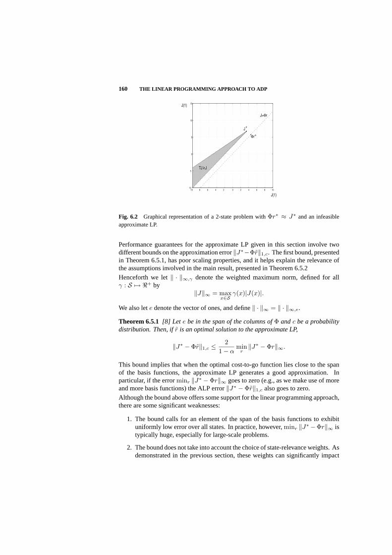
160 THE LINEAR PROGRAMMING APPROACH TO ADP
10 8 6 4 2 0 2 4 6 8 1010
5
0
5
10
15
J∗
Φr∗
J=Φr
TJ J>
J(1)
J(1)
Fig. 6.2 Graphical representation of a 2-state problem withΦr∗ ≈ J∗ and an infeasibleapproximate LP.
Performance guarantees for the approximate LP given in this section involve twodifferent bounds on the approximation error‖J∗−Φr‖1,c. The first bound, presentedin Theorem 6.5.1, has poor scaling properties, and it helps explain the relevance ofthe assumptions involved in the main result, presented in Theorem 6.5.2
Henceforth we let‖ · ‖∞,γ denote the weighted maximum norm, defined for allγ : S 7→ <+ by
‖J‖∞ = maxx∈S
γ(x)|J(x)|.
We also lete denote the vector of ones, and define‖ · ‖∞ = ‖ · ‖∞,e.
Theorem 6.5.1 [8] Let e be in the span of the columns ofΦ andc be a probabilitydistribution. Then, ifr is an optimal solution to the approximate LP,
‖J∗ − Φr‖1,c ≤ 21− α
minr‖J∗ − Φr‖∞.
This bound implies that when the optimal cost-to-go function lies close to the spanof the basis functions, the approximate LP generates a good approximation. Inparticular, if the errorminr ‖J∗ −Φr‖∞ goes to zero (e.g., as we make use of moreand more basis functions) the ALP error‖J∗ − Φr‖1,c also goes to zero.
Although the bound above offers some support for the linear programming approach,there are some significant weaknesses:
1. The bound calls for an element of the span of the basis functions to exhibituniformly low error over all states. In practice, however,minr ‖J∗−Φr‖∞ istypically huge, especially for large-scale problems.
2. The bound does not take into account the choice of state-relevance weights. Asdemonstrated in the previous section, these weights can significantly impact

APPROXIMATION ERROR BOUNDS 161
the quality of the approximate cost-to-go function. A more meaningful boundshould take them into account.
To set the stage for the development of an improved bound, let us establish somenotation. LetH be the operator given by
(HV )(x) = maxa∈Ax
∑
y∈SPa(x, y)V (y),
for all V : S 7→ <. For anyV , (HV )(x) represents the maximum expected value ofV (Y ) if the current state isx andY is a random variable representing the next state.
For eachV : S 7→ <, we define a scalarβV given by
βV = maxx
α(HV )(x)V (x)
. (6.8)
Definition 6.5.1 (Lyapunov function) We callV : S 7→ <+ a Lyapunov function ifβV < 1.
Existence of a Lyapunov function translates into the condition that there existV > 0andβ < 1 such thatα(HV )(x) ≤ βV (x), ∀x ∈ S. If α were equal to1, this wouldlook like a Lyapunov stability condition: the maximum expected value(HV )(x) atthe next time step must be less than the current valueV (x). In general,α is less than1, and this introduces some slack in the condition.
We are now ready to state the main result of this section. For any given functionVmappingS to positive reals, we use1/V as shorthand for a functionx 7→ 1/V (x).
Theorem 6.5.2 [8] Let r be a solution of the approximate LP. Then, for anyv ∈ <K
such thatΦv is a Lyapunov function, we have
‖J∗ − Φr‖1,c ≤ 2cT Φv
1− βΦvmin
r‖J∗ − Φr‖∞,1/Φv. (6.9)
Let us now discuss how Theorem 6.5.2 addresses the shortcomings of Theorem 6.5.1.
1. The norm‖ · ‖∞ appearing in Theorem 6.5.1 is undesirable largely becauseit does not scale well with problem size. In particular, for large problems,the optimal cost-to-go function can take on huge values over some (possiblyinfrequently visited) regions of the state space, and so can approximation errorsin such regions. Observe that the maximum norm of Theorem 6.5.1 has beenreplaced in Theorem 6.5.2 by‖ · ‖∞,1/Φv. Hence, the error at each state isnow weighted by the reciprocal of the Lyapunov function value. This shouldto some extent alleviate difficulties arising in large problems. In particular, theLyapunov function should take on large values in undesirable regions of thestate space — regions whereJ∗ is large. Hence, division by the Lyapunovfunction acts as a normalizing procedure that scales down errors in such regions.
162 THE LINEAR PROGRAMMING APPROACH TO ADP
2. As opposed to the bound of Theorem 6.5.1, the state-relevance weights doappear in the new bound. In particular, there is a coefficientcT Φv scalingthe right-hand side. In general, if the state-relevance weights are chosenappropriately, we expect thatcT Φv will be reasonably small and independentof problem size. Section 6.6 provides further qualification of this statement anda discussion of approaches to choosingc in the context of a concrete example.
It is important to note that the Lyapunov functionΦv plays a central role in thebound of Theorem 6.5.2. Its choice influences three terms on the right-hand-side ofthe bound: the errorminr ‖J∗ − Φr‖∞,1/Φv, the term1/(1 − βΦv), and the innerproductcT Φv with the state-relevance weights. An appropriately chosen Lyapunovfunction should make all three of these terms relatively small. Furthermore, for thebound to be useful in practical contexts, these terms should not grow much withproblem size. We illustrate choices of Lyapunov functions via an application to amulticlass queueing problem, in the next section.
6.6 APPLICATION TO QUEUEING NETWORKS
This section presents an example involving choices of state-relevance weights andLyapunov functions in a multiclass queueing problem. The intention is to illus-trate more concretely how state-relevance weights and Lyapunov functions mightbe chosen and show that reasonable choices lead to practical error bounds that areindependent of the number of states and of the number of state variables.
Consider a queueing network withd queues and finite buffers of size B. We assumethat the number of exogenous arrivals occuring in any time step has expected valueless than or equal toAd, for a finiteA. The statex ∈ <d indicates the number of jobsin each queue. The cost per stage incurred at statex is given byg(x) = 1
d
∑di=1 xi,
the average number of jobs per queue.
Let us first consider the optimal cost-to-go functionJ∗ and its dependency on thenumber of state variablesd. The goal is to establish bounds onJ∗ that will offer someguidance on the choice of a Lyapunov functionV that keeps the errorminr ‖J∗ −Φr‖∞,1/V small. SinceJ∗ ≥ 0 only upper bounds will be derived.
Instead of carrying the buffer sizeB throughout calculations, attention is restrictedto the infinite buffer case. The optimal cost-to-go function for the finite buffer caseshould be bounded above by that of the infinite buffer case, as having finite bufferscorresponds to having jobs arriving at a full queue discarded at no additional cost.
We haveEx [|xt|] ≤ |x|+ Adt,
since the expected total number of jobs at timet cannot exceed the total number ofjobs at time 0 plus the expected number of arrivals between 0 andt, which is lessthan or equal toAdt. Ex stands for the expected value conditioned onx0 = x, and

APPLICATION TO QUEUEING NETWORKS 163
|x| = ∑di=1 xi. It follows from this inequality that
Ex
[ ∞∑t=0
αt|xt|]
=∞∑
t=0
αtEx [|xt|]
≤∞∑
t=0
αt(|x|+ Adt)
=|x|
1− α+
Ad
(1− α)2. (6.10)
The first equality holds because|xt| ≥ 0 for all t; by the monotone convergencetheorem, we can interchange the expectation and the summation. We concludefrom (6.10) that the optimal cost-to-go function in the infinite buffer case should bebounded above by a linear function of the state; in particular,
0 ≤ J∗(x) ≤ ρ1
d|x|+ ρ0,
for some positive scalarsρ0 andρ1 independent of the number of queuesd.
As discussed before, the optimal cost-to-go function in the infinite buffer case pro-vides an upper bound for the optimal cost-to-go function in the case of finite buffersof sizeB. Therefore, the optimal cost-to-go function in the finite buffer case shouldbe bounded above by the same linear function regardless of the buffer sizeB.
We will establish bounds on the terms involved in the error bound of Theorem 6.5.2.Consider a Lyapunov functionV (x) = 1
d |x|+ C for some constantC > 0. Then
minr‖J∗ − Φr‖∞,1/V ≤ ‖J∗‖∞,1/V
≤ maxx≥0
ρ1|x|+ dρ0
|x|+ dC
≤ ρ1 +ρ0
C,
and the bound above is independent of buffer size and number of queues.
Consider the termβV . We have
α(HV )(x) ≤ α
( |x|+ Ad
d+ C
)
≤ V (x)
(α +
αA|x|d + C
)
≤ V (x)(
α +αA
C
),

164 THE LINEAR PROGRAMMING APPROACH TO ADP
and it is clear that, forC sufficiently large and independent ofd, there is a scalarβ < 1 independent ofd such thatαHV ≤ βV , and therefore 1
1−βVis uniformly
bounded onB andd.
Finally, consider the termcT V . Under some stability assumptions, the tail of thesteady-state distribution will have an upper bound with geometric decay [4]. This
motivates choosingc(x) =(
1−ξ1−ξB+1
)d
ξ|x|. The state-relevance weightsc are equiv-
alent to the conditional joint distribution ofd independent and identically distributedgeometric random variables conditioned on the event that they are all less thanB +1.Therefore,
cT V = E
[1d
d∑
i=1
Xi + C | Xi < B + 1, i = 1, ..., d
]
< E [X1] + C
=ξ
1− ξ+ C,
whereXi, i = 1, ..., d are identically distributed geometric random variables withparameter1−ξ. It follows thatcT V is uniformly bounded over buffer size and numberof queues. We conclude that the error produced by approximate linear programmingin this problem is uniformly bounded on the size and dimension of the state space.
6.7 AN EFFICIENT CONSTRAINT SAMPLING SCHEME
While the approximate LP may involve only a small number of variables, there isa potentially intractable number of constraints — one per state-action pair. Thissection describes a tractable approximation to the approximate LP: the reduced linearprogram (reduced LP).
Generation of a reduced LP relies on three objects: (1) a constraint sample sizem,(2) a probability measureψ over the set of state-action pairs, and (3) a boundingsetN ⊆ <K . The probability measureψ represents a distribution from whichconstraints are sampled. In particular, we consider a setX of m state-action pairs,each independently sampled according toψ. The setN is a parameter that restrictsthe magnitude of the reduced LP solution. This set should be chosen such that itcontainsΦr. The reduced LP is defined by
max cT Φrs.t. ga(x) + α
∑y Pa(x, y)(Φr)(y) ≥ (Φr)(x), ∀(x, a) ∈ X
r ∈ N .(6.11)
Let r be an optimal solution of the approximate LP and letr be an optimal solutionof the reduced LP. In order for the solution of the reduced LP to be meaningful,
AN EFFICIENT CONSTRAINT SAMPLING SCHEME 165
‖J∗−Φr‖1,c should close to‖J∗−Φr‖1,c. This is formalized as a requirement that
Prob (‖J∗ − Φr‖1,c ≤ ‖J∗ − Φr‖1,c + ε‖J∗‖1,c) ≥ 1− δ,
whereε > 0 is an error tolerance parameter andδ > 0 parameterizes a level ofconfidence1− δ. The main result of this section is the characterization of a tractablesample sizem that is sufficient for meeting such a requirement. In particular, it isshown that, ifψ andN are well-chosen, an error tolerance ofε can be accommodatedwith confidence1− δ given a sample sizem that grows as a polynomial inK, 1/ε,andlog 1/δ, and isindependentof the total number of approximate LP constraints.
The analysis is based on the notion of near-feasibility. Given a probability distributionψ over state-action pairs and a scalarε > 0, r is said to be(ψ, ε)-near-feasible if
ψ ((x, a) : (TaΦr)(x) < (Φr)(x)) < ε,
i.e., the set of constraints violated byr has measure less than or equal toε.
The following theorem is a direct application of results on uniform convergenceof empirical probabilities [14, 30], and establishes that only a tractable number ofconstraints needs to be considered in order to ensure near-feasibility.
Theorem 6.7.1 [9] Let 0 < δ < 1, 0 < ε < 1 be given constants and letW be a setformed by samplingm i.i.d. state-action pairs sampled fromψ. Then if
m ≥ 32ε2
[ln 8 + ln
1δ
+ k
(ln
16e
ε+ ln ln
16e
ε
)], (6.12)
we have
supr:(TaΦr)(x)≥(Φr)(x)
∀(x,a)∈W
ψ ((x, a) : (TaΦr)(x) < (Φr)(x)) ≤ ε, (6.13)
with probability at least1− δ.
It is easy to see that near-feasibility is not enough to ensure a small error if thesolution of the reduced LP involves arbitrarily large violations of the non–sampledconstraints. The next result presents conditions that enable a graceful bound on theerror in the approximation of the cost-to-go function incurred by solving the reducedLP instead of the approximate LP.
Let us first introduce certain constants and functions involved in our error bound.
For any Lyapunov functionV , we define a family of probability distributions on thestate spaceS, given by
µu,c,V (x) =µu,c(x)V (x)
µTu,cV
.

166 THE LINEAR PROGRAMMING APPROACH TO ADP
We also define a distribution over state-action pairs
ψu,c,V (x, a) =µu,c,V (x)|Ax| , ∀a ∈ Ax.
Finally, let the constantsA andθ be given by
A = maxx|Ax|
and
θ =µT
u∗V
cT J∗supr∈N
‖J∗ − Φr‖∞,1/V .
Theorem 6.7.2 is the main result of this section — a bound on the approximationerror introduced by constraint sampling.
Theorem 6.7.2 [9] Let u∗ be an optimal policy andX be a (random) set ofm state-action pairs sampled independently according to the distributionψu∗,c,V (x, a), forsome Lyapunov functionV , where
m ≥ 512A2θ2
(1− α)2ε2
[ln
8δ
+ K ln(
64Aθe
(1− α)εln
64Aθe
(1− α)ε
)]. (6.14)
Let r be an optimal solution of the approximate LP that is inN , and let r be anoptimal solution of the corresponding reduced LP. Ifr ∈ N then, with probability atleast1− δ, we have
‖J∗ − Φr‖1,c ≤ ‖J∗ − Φr‖1,c + ε‖J∗‖1,c. (6.15)
Certain aspects of Theorem 6.14 deserve further consideration. A major weaknessof Theorem 6.14 is that it relies on an idealized choice ofψ. In particular, thechoice assumes knowledge of an optimal policy. Alas, we typically do not know anoptimal policy — that is what we are after in the first place. Nevertheless, the resultprovides guidance on what makes a desirable choice of distribution. The spirit hereis analogous to one present in the importance sampling literature. In that context,the goal is to reduce variance in Monte Carlo simulation through intelligent choiceof a sampling distribution and appropriate distortion of the function being integrated.Characterizations of idealized sampling distributions guide the design of heuristicsthat are ultimately implemented.
The setN also plays a critical role in the bound. It influences the value ofθ, and anappropriate choice is necessary in order for this term to scale gracefully with problemsize. Ideally, given a class of problems, there should be a mechanism for generatingN such thatθ grows no faster than a low-order polynomial function of the numberof basis functions and the number of state variables. As illustrated later through anexample involving controlled queueing networks, we expect that it will be possibleto design effective mechanisms for selectingN for practical classes of problems.

AN EFFICIENT CONSTRAINT SAMPLING SCHEME 167
Finally, the number of sampled constraints grows polynomially with the maximumnumber of actions available per stateA, which makes the proposed approach inap-plicable to problems with a large number of actions per state. In [9], it is shown thatcomplexity in the action space can be exchanged for complexity in the state space,so that such problems can be recast in an amenable format.
Note that the sample complexity bounds in Theorems 6.7.1 and 6.7.2 are loose. Theemphasis is on showing that the number of required samples can be independent ofthe total number of constraints and can scale gracefully with respect to the numberof variables. Furthermore, the emphasis is on a general result that holds for a broadclass of MDPs, therefore special regularities associated with particular choices ofbasis functions or specific problems are not being exploited. In the presence ofsuch special structure, it may be possible to provide much tighter bounds or evenmethods for exact solution of the approximate LP. Examples of how problem-specificstructure may lead to tractable solution of the approximate LP can be found in theliterature in applications such as queueing networks [21], factored MDP’s [17, 24]or the traveling salesman problem [16]. Exploitation of particular properties andregularities of the problem at hand is obviously useful and the constraint samplingscheme is not meant as a substitute for that. The significance of the results presentedhere is that they suggest viability of the linear programming approach to approximatedynamic programming even in the absence of such favorable special structure.
6.7.1 Example: Controlled Queueing Networks
In order for the error bound (6.15) to be useful, the parameter
θ =µT
u∗V
cT J∗supr∈N
‖J∗ − Φr‖∞,1/V ,
should scale gracefully with problem size. We anticipate that for many relevantclasses of MDPs, natural choices ofV andN will ensure this. This section illustratesthis point through an example involving controlled queueing networks. The keyresult is Theorem 6.7.3, which establishes that — given certain reasonable choicesof Φ,N , andV — θ grows at most linearly with the number of queues.
We consider classes of problems denoted byQ(ξ, α, λ), with the following interpre-tation. Each problem instanceQ ∈ Q(ξ, α, λ) corresponds to a queueing controlproblem of the form described in Section 6.6 and identified by a quadruple:
• number of queuesdQ ≥ 1;
• buffer sizeBQ ≥ dQξ/(1− ξ);
• action setsAQ· ;
• transition probabilitiesPQ· (·, ·).
EachQ ∈ Q(ξ, α, λ) involves a discount factorα, and the expected number ofarrivals in any time step is less than or equal toλd.

168 THE LINEAR PROGRAMMING APPROACH TO ADP
Let u∗Q and J∗Q denote an optimal policy and the optimal cost-to-go function fora problem instanceQ. We consider approximatingJ∗Q by a linear combination of
basis functionsφQk (x) = xk, k = 1, . . . , dQ andφQ
dQ+1(x) = 1, using the followingapproximate LP:
maximize∑
x∈S cQ(x)(∑dQ+1
k=1 rkxk + rd+1
)
subject to 1dQ
∑dQ
i=1 xi + α∑
y∈S PQa (x, y)
(∑dQ
k=1 rkyk + rdQ+1
)
≥ ∑dQ
k=1 rkxk + rdQ+1, ∀x ∈ SQ, a ∈ AQx ,
(6.16)whereSQ = 0, . . . , BQdQ and the state-relevance weights are given by
cQ(x) =ξ−
∑dQi=1 xi
∑y∈SQ
ξ−∑dQ
i=1 yi
.
The number of constraints imposed by the approximate LP (6.16) grows exponentiallywith the number of queuesdQ. For even a moderate number of queues (e.g., ten),the number of constraints becomes unmanageable. Constraint sampling offers anapproach to alleviating this computational burden.
Formulating a reduced LP, given a problem instanceQ, requires defining a constraintsetNQ and a sampling distributionψQ. LetNQ to be the set of vectorsr ∈ <d+1
that satisfy the following linear constraints:
rdQ+1 ≤ λ
(1− α)2, (6.17)
BQrk + rdQ+1 ≤ BQ
(1− α)dQ+
λ
(1− α)2∀k = 1, . . . , dQ, (6.18)
(ξ
1− ξ− ξBQ+1(BQ + 1)
1− ξBQ+1
) dQ∑
k=1
rk + rdQ+1 ≥ 0. (6.19)
Note that the resulting reduced LP is a linear program withm + dQ + 2 constraints,wherem is the number of sampled ALP constraints.
It turns out thatNQ has two desirable properties: it contains optimal solutions of theALP (6.16) and is uniformly bounded overQ(ξ, α, λ).
Lemma 6.7.1 [9] For each ξ ∈ (0, 1), α ∈ (0, 1), and λ ∈ (0,∞) and eachQ ∈ Q(ξ, α, λ),NQ contains every optimal solution of the ALP (6.16).
Lemma 6.7.2 [9] For each ξ ∈ (0, 1), α ∈ (0, 1), andλ ∈ (0,∞), there exists ascalarCξ,α,λ such that
supr∈NQ
‖r‖∞ ≤ Cξ,α,λ,
for all Q ∈ Q(ξ, α, λ).

DISCUSSION 169
Now consider the distributionψQ = ψu∗Q,VQ, where
VQ(x) =1
dQ(1− α)
dQ∑
i=1
xi +2λ
(1− α)2. (6.20)
The following lemma establishes thatVQ is an optimal-policy Lyapunov function.
Lemma 6.7.3 [9] For each ξ ∈ (0, 1), α ∈ (0, 1) and λ ∈ (0,∞) and eachQ ∈Q(ξ, α, λ), VQ is an optimal-policy Lyapunov function.
Recall that the bound on sample complexity for the reduced LP, given by Eq. (6.14),is affected by a parameterθ. In the context of controlled queueing networks, we havea parameterθQ for each problem instanceQ ∈ Q(ξ, α, λ):
θQ =µT
u∗QVQ
cTQJ∗Q
supr∈NQ
‖J∗Q − ΦQr‖∞,1/VQ.
The final result presented here establishes thatθQ can be bounded above by a linearfunction of the number of queues.
Theorem 6.7.3 For eachξ ∈ (0, 1), α ∈ (0, 1), and λ ∈ (0,∞), there exists ascalarCξ,α,λ such thatθQ ≤ Cξ,α,λdQ.
Combining this theorem with the sample complexity bound of Theorem 6.7.2, itfollows that for anyQ ∈ Q(ξ, α, λ), a number of samples
m = O
(AQdQ
(1− α)ε
(dQ ln
AQdQ
(1− α)ε+ ln
1δ
)),
whereAQ = maxx∈SQ|AQ
x |, suffices to guarantee that
‖J∗Q − ΦQr‖1,cQ ≤ ‖J∗Q − ΦQr‖1,cQ + ε‖J∗Q‖1,cQ ,
with probability1− δ. Hence, the number of samples grows at most quadratically inthe number of queues.
6.8 DISCUSSION
The present analysis represents a step toward making approximate linear program-ming a streamlined approach to large-scale dynamic programming. It offers a betterunderstanding of the role of state-relevance weights and insights on how they canbe chosen so as to indirectly optimize performance of the policy being generated.The analysis also offers guarantees for the error in the approximation of the optimalcost-to-go function — approximate LP produces approximations that are comparableto the best that could have been achieved with the given selection of basis functions.
170 THE LINEAR PROGRAMMING APPROACH TO ADP
The performance and approximation error bounds enable us to predict the scalingproperties of approximate LP for broadly defined classes of problems, as illustratedby the study of multiclass queueing networks. Finally, this chapter presents generalapproach to dealing with the large number of constraints involved in the approximateLP, which one can resort to in the absence of problem-specific structure allowing forexact solution of the approximate LP.
There are a number of directions to be pursued in the further development of approx-imate linear programming. We mention a few:
Large discount factors and average-cost criterion.This chapter investigated howapproximate linear programming scales with the size and dimension of the state spaceof the system, but there is no consideration of how the algorithm scales as the discountfactor increases. The current performance and error bounds do not scale well withdiscount factor; in particular, the error bound (6.9) should scale with1/(1−α)2. TheLyapunov function analysis used to develop the bound also seems overly restrictivein the average-cost setting, as in this case it requires stability of all policies. Initialexploration of the average-cost case can be found in [10]. It is shown that a naiveapproximate LP formulation of the average-cost problem, which follows directlyfrom the discounted-cost version, may lead to undesirable behavior of approximateLP, and therefore a more sophisticated version of the algorithm is required.
Adaptive choice of state-relevance weights.The performance bound in Theorem6.4.1 suggests finding a weight vectorr such thatΦr minimizes
‖Φr − J∗‖1,µν,ur,
whereν is the estimate for the initial state distribution. By contrast, approximatelinear programming minimizes
‖Φr − J∗‖1,c,
with state-relevance weightsc determined by the user, and we have strong guaranteesfor the error‖Φr−J∗‖1,c at the optimal solutionr of the approximate LP. Ifc is closeto µν,ur , combining the performance and error bounds leads to a strong guaranteeon the performance of the policy generated by approximate LP. These observationssuggest an iterative scheme for adaptive choices of state-relevance weights:
1. Start with an arbitrary policyu0, let k = 0;
2. Solve the approximate LP with state-relevance weightsµν,ukto determine a
new policyuk+1;
3. Letk = k + 1 and go back to step 2.
Questions regarding the convergence of such a scheme and how much it wouldimprove performance must be addressed. Note that the above algorithm is basedon the assumption that a initial distributionν over the states is given. Runningapproximate linear programming online also raises the possibility of adapting the

DISCUSSION 171
initial distributionν to reflect the current state of the system, so that if at thekth ofthe approximate LP the system is at statex, we may setν = 1x.
Robustness to model uncertainty.In principle, approximate linear programmingrequires explicit knowledge of the costs and transition probabilities in the system.This requirement can be relaxed by noting that, in fact, transition probabilities appearin the approximate LP only through the expected values
∑y
Pa(x, y)Φ
of the basis functions evaluated at the next stateXk+1 given the current stateXk = xof the system. Hence the approximate LP can be implemented without major changesif there is access to a system simulator that takes as input any statex and produces anext statey distributed according toPa(x, ·). A more interesting situation arises in thecase where such a simulator is not available, but rather one must learn from onlineobservations of the system, and possibly adapt to changes in the system behaviorover time. In this case, it would be interesting to identify whether it is possibleto continually update the approximate LP parameters, easily determine when it isnecessary to re-solve the LP, and exploit knowledge of previous solutions to speedup computations in the approximate LP.
Basis function generation. A central issue in any approximate dynamic program-ming algorithm that has not been addressed in this chapter regards the choice ofbasis functions. Note that including additional basis functions in the approximate LPcorresponds to adding extra columns, hence it may be possible to apply general linearprogramming column generation techniques to approximate linear programming inorder to generate new basis functions leading to improvement in the approximationerror. For an initial exploration of this idea, see [23], where it is shown how theLagrange multipliers of the approximate LP can be used to assess whether addingany given new basis functions should lead to improvement in the approximation.
Appropriate distributions for constraint sampling. Theorem 6.7.2, involves anassumption that states are sampled according to distributionµu∗ for some optimalpolicyu∗. In general it is not possible to computeµu∗ in practice, without knowledgeof the optimal policyu∗; hence to constraints have to be sampled according to analternative distributionµ. Intuitively, if µ is reasonably close toµu∗ , the reduced LPshould still produce meaningful answers. How closeµ andµu∗ have to be and howto choose an appropriateµ are still open questions. As a simple heuristic, noting thatµ∗(x) → c(x) asα → 0, one might chooseµ = c. This choice is also justified bythe realization that, in many applications,c is an estimate forπu∗, and ifc = πu∗ , itis also true thatµu∗ = c = πµ∗ .

Bibliography
1. D. Adelman,A price-directed approach to stochastic inventory/routing,Preprint,2002.
2. D. Adelman,Price-directed replenishment of subsets: Methodology and itsapplication to inventory routing,Preprint, 2002.
3. D. Bertsekas and J.N. Tsitsiklis,Neuro-Dynamic Programming,Athena Scien-tific, 1996.
4. D. Bertsimas, D. Gamarnik, and J.N. Tsitsiklis, “Performance of multiclassMarkovian queueing networks via piecewise linear Lyapunov functions,”Annalsof Applied Probability,11(4):1384–1428, 2001.
5. V. Borkar, “A convex analytic approach to Markov decision processes,”Proba-bility Theory and Related Fields,78:583–602, 1988.
6. R.H. Crites and A.G. Barto, “Improving elevator performance using reinforce-ment learning,”Advances in Neural Information Processing Systems,volume 8,1996.
7. D.P. de Farias,The Linear Programming Approach to Approximate DynamicProgramming,PhD thesis, Stanford University, 2002.
8. D.P. de Farias and B. Van Roy, “The linear programming approach to approximatedynamic programming,” To appear inOperations Research,2001.
9. D.P. de Farias and B. Van Roy, “On constraint sampling in the linear programmingapproach to approximate dynamic programming,” Conditionally accepted toMathematics of Operations Research,2001.
10. D.P. de Farias and B. Van Roy, “Approximate linear programming for average-cost approximate dynamic programming,”Advances in Neural Information Pro-cessing Systems,volume 15, 2003.
11. G. de Ghellinck, “Les problemes de decisions sequentielles,”Cahiers du Centred’Etudes de Recherche Operationnelle,2:161–179, 1960.
12. E.V. Denardo, “On linear programming in a Markov decision problem,”Man-agement Science,16(5):282–288, 1970.
172

BIBLIOGRAPHY 173
13. F. D’Epenoux, “A probabilistic production and inventory problem,”ManagementScience, 10(1):98–108, 1963.
14. R.M. Dudley,Uniform Central Limit Theorems,Cambridge University Press,Cambridge, 1998.
15. G. Gordon,Approximate Solutions to Markov Decision Processess,PhD thesis,Carnegie Mellon University, 1999.
16. M. Grotschel and O. Holland, “Solution of large-scale symmetric travellingsalesman problems,”Mathematical Programming,51:141–202, 1991.
17. C. Guestrin, D. Koller, and R. Parr, “Efficient solution algorithms for factoredMDPs,” To appear in Journal of Artificial Intelligence Research, 2002.
18. A. Hordijk and L.C.M. Kallenberg, “Linear programming and Markov decisionchains,”Management Science,25:352–362, 1979.
19. F. Longstaff and E.S. Schwartz, “Valuing American options by simulation: Asimple least squares approach,”The Review of Financial Studies,14:113–147,2001.
20. A.S. Manne, “Linear programming and sequential decisions,”Management Sci-ence,6(3):259–267, 1960.
21. J.R. Morrison and P.R. Kumar, “New linear program performance boundsfor queueing networks,”Journal of Optimization Theory and Applications,100(3):575–597, 1999.
22. I.C. Paschalidis and J.N. Tsitsiklis, “Congestion-dependent pricing of networkservices,”IEEE/ACM Transactions on Networking,8(2):171–184, 2000.
23. P. Poupart, R. Patrascu, D. Schuurmans, C. Boutilier, and C. Guestrin, “Greedylinear value function approximation for factored Markov decision processes,”The Eighteenth National Conference on Artificial Intelligence,2002.
24. D. Schuurmans and R. Patrascu, “Direct value-approximation for factoredMDPs,” Advances in Neural Information Processing Systems,volume 14, 2001.
25. P. Schweitzer and A. Seidmann, “Generalized polynomial approximations inMarkovian decision processes,”Journal of Mathematical Analysis and Applica-tions,110:568–582, 1985.
26. G.J. Tesauro, “Temporal difference learning and TD-gammon,”Communicationsof the ACM,38:58–68, 1995.
27. M. Trick and S. Zin, “A linear programming approach to solving dynamic pro-grams,” Unpublished manuscript, 1993.
28. M. Trick and S. Zin, “Spline approximations to value functions: A linear pro-gramming approach,”Macroeconomic Dynamics,1, 1997.

174 BIBLIOGRAPHY
29. J.N. Tsitsiklis and B. Van Roy, “Regression methods for pricing complexAmerican-style options,”IEEE Transactions on Neural Networks,12(4):694–703, 2001.
30. M. Vidyasagar,A Theory of Learning and Generalization,Springer, London,1997.
31. W. Zhang and T.G. Dietterich, “High-performance job-shop scheduling with atime-delay TD(λ) network,” Advances in Neural Information Processing Sys-tems,volume 8, 1996.
7 Reinforcement Learning in Large,High Dimensional State Spaces
GREG GRUDIC and LYLE UNGARUniversity of Colorado at Boulder University of Pennsylvania
Editor’s Summary: The previous chapter addresses the “curse of dimensionality”by treating ADP as the dual of the linear programming problem and introduces themethod known as approximate linear programming. This chapter presents anothermethod for dealing with the “curse of dimensionality,” the policy gradient reinforce-ment learning framework. The Action Transition Policy Gradient (ATPG) algorithmpresented here estimates a gradient in the policy space that increases reward. Fol-lowing a brief motivation the authors present their algorithm in detail and discuss itsproperties. Finally, detailed experimental results are presented to show the types ofproblems that the algorithm can be applied to and what type of performance can beexpected. Another algorithm, Boundary Localized Reinforcement Learning, is alsodiscussed in this chapter. This is a mode switching controller that can be used toincrease the rate of convergence.
7.1 INTRODUCTION
In Reinforcement Learning (RL) an agent uses a trial and error strategy to explore itsenvironment with the goal of learning to maximize some (often infrequent) reward.This trial and error learning process is governed by stochastic search, which definesa probability distribution of actions taken during exploration. This type of stochasticsearch strategy has proven effective in many RL applications that intrinsically havelow dimensional state spaces [14].
However, applying a stochastic search strategy (or any poorly directed search strat-egy) to higher dimensional problems is problematic because, in general, the searchspace grows exponentially with the number of state variables. As a consequence,the computational cost and the time to convergence of reinforcement learning canquickly become impractical as the dimension of the problem increases. Function ap-proximation techniques have been proposed for learning generalizations across large
175

176 RL IN LARGE, HIGH DIMENSIONAL STATE SPACES
state spaces, as one possible solution to this curse of dimensionality problem in RL.However, even when function approximation techniques successfully generalize, thedimension of the search remains unchanged, and its computational cost and rate ofconvergence can still be impractical.
The goal of this chapter is to present a detailed summary of our recent effortsin addressing the convergence problems of RL in large state spaces. The maintheme of our efforts has been to systematically direct search in ways that allowquick convergence tolocally optimal policies. We specifically focus our theoryat convergence tolocal optimums because, in the large problem domains we areinterested in, convergence to globally optimal policies is simply not possible. Insupport of this claim, we pose the following question: can any human or animal claimto have achieved a globally optimal solution for how to live life? The answer to thisquestion obviously is no, and although our systems do not approach the complexity ofliving animals, they never the less cannot hope to achieve globally optimal policies.One example of this is a real mail delivery robot, where obstacles it must avoidcontinually move around (e.g. humans), sensors are noisy, actuators don’t alwaysperform the same, task parameters change, and the size of the state space can bethousands of real valued variables (vision sensors, sonar sensors, collision sensors,etc). Given all these uncertainties and the large problem space, globally optimalcontrol polices are simply not reasonable.
The approach to RL advocated here has three specific properties. First we formulateour solution within the Policy Gradient Reinforcement Learning (PGRL) framework,where the agent estimates a gradient in policy space which increases reward, andincrementally updates it’s policy along this gradient. There are a number of formu-lations of PGRL, all of which have theoretical guarantees to locally optimal policies[12, 5, 6, 2, 26]. In Section 7.1.1, we present our motivation for using this frameworkover the more traditional value function RL framework [21].
The key to effective learning in PGRL is efficiently obtaining accurate estimates ofthe performance gradient. Therefore, the second property of our RL formulation isthat we propose a PGRL algorithm, called Action Transition Policy Gradient (ATPG),which restricts estimates of the performance gradient to coincide with states wherethe agent changes from executing one action to another [2]. As argued below (seeSection 7.1.2), this formulation reduces the variance in policy gradient estimates andgreatly improves the rate of convergence of PGRL.
The third, and final, key property of our RL formulation is that we further reduce thecomputational cost of search in high dimensional spaces by restricting the agent’spolicy to a mode switching controller, which restricts the search to very limitedregions of the state space [1]. The size of the search region bounds the computationalcost of RL. Intuitively, the smaller the search region, the lower the computational costof learning, making it possible to apply RL to very high dimensional problems. Thisformulation of RL is called Boundary Localized Reinforcement Learning (BLRL)and is motivated in Section 7.1.3.
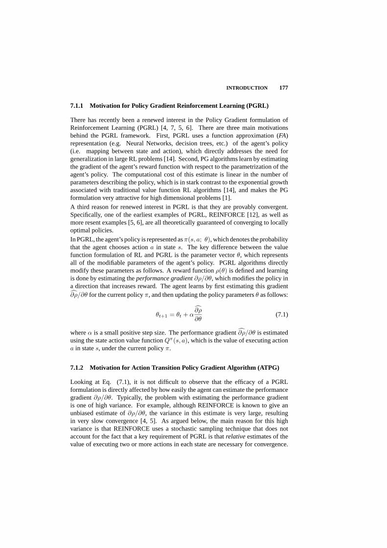
INTRODUCTION 177
7.1.1 Motivation for Policy Gradient Reinforcement Learning (PGRL)
There has recently been a renewed interest in the Policy Gradient formulation ofReinforcement Learning (PGRL) [4, 7, 5, 6]. There are three main motivationsbehind the PGRL framework. First, PGRL uses a function approximation (FA)representation (e.g. Neural Networks, decision trees, etc.) of the agent’s policy(i.e. mapping between state and action), which directly addresses the need forgeneralization in large RL problems [14]. Second, PG algorithms learn by estimatingthe gradient of the agent’s reward function with respect to the parametrization of theagent’s policy. The computational cost of this estimate is linear in the number ofparameters describing the policy, which is in stark contrast to the exponential growthassociated with traditional value function RL algorithms [14], and makes the PGformulation very attractive for high dimensional problems [1].
A third reason for renewed interest in PGRL is that they are provably convergent.Specifically, one of the earliest examples of PGRL, REINFORCE [12], as well asmore resent examples [5, 6], are all theoretically guaranteed of converging to locallyoptimal policies.
In PGRL, the agent’s policy is represented asπ(s, a; θ), which denotes the probabilitythat the agent chooses actiona in states. The key difference between the valuefunction formulation of RL and PGRL is the parameter vectorθ, which representsall of the modifiable parameters of the agent’s policy. PGRL algorithms directlymodify these parameters as follows. A reward functionρ(θ) is defined and learningis done by estimating theperformance gradient∂ρ/∂θ, which modifies the policy ina direction that increases reward. The agent learns by first estimating this gradient∂ρ/∂θ for the current policyπ, and then updating the policy parametersθ as follows:
θt+1 = θt + α∂ρ
∂θ(7.1)
whereα is a small positive step size. The performance gradient∂ρ/∂θ is estimatedusing the state action value functionQπ(s, a), which is the value of executing actiona in states, under the current policyπ.
7.1.2 Motivation for Action Transition Policy Gradient Algorithm (ATPG)
Looking at Eq. (7.1), it is not difficult to observe that the efficacy of a PGRLformulation is directly affected by how easily the agent can estimate the performancegradient∂ρ/∂θ. Typically, the problem with estimating the performance gradientis one of high variance. For example, although REINFORCE is known to give anunbiased estimate of∂ρ/∂θ, the variance in this estimate is very large, resultingin very slow convergence [4, 5]. As argued below, the main reason for this highvariance is that REINFORCE uses a stochastic sampling technique that does notaccount for the fact that a key requirement of PGRL is thatrelativeestimates of thevalue of executing two or more actions in each state are necessary for convergence.

178 RL IN LARGE, HIGH DIMENSIONAL STATE SPACES
Therefore, an agent using REINFORCE must pass through the same set of states manytimes, and hope that its stochastic policy executes a sufficient number of differentactions in each state to obtain this relative value estimate.
Function approximation representations ofQπ(s, a) (i.e. knowing the value ofexecuting every action in every state under the current policy) have been proposedas one way of decreasing the variance in estimating∂ρ/∂θ. Given Qπ(s, a), therelative value of executing each action in each state is explicitly known [5, 6]. Thisapproach seeks to build function approximation representationsf(s, a) ≈ Qπ(s, a),and then use these approximations instead of direct samples ofQπ(s, a) to estimate∂ρ/∂θ. In [5, 6] it is shown that if the form off(s, a) is restricted appropriately,then the resulting PG algorithm is guaranteed to converge to a locally optimal policy.However, as argued below, function approximation approaches to policy gradientsare not necessarily optimal.
How PGRL algorithms should be formulated to give fast convergence to locallyoptimal solutions is an important ongoing area of research [3]. In PGRL formulationsperformance gradient estimates typically have the following form:
∂ρ
∂θ= f
([Q (s1, a1)− b (s1)
], ...,
[Q (sT , aT )− b (sT )
])(7.2)
whereQ (si, ai) is the estimate of the value of executing actionai in statesi (i.e.the state action value function),b(si) the bias subtracted fromQ (si, ai) in statesi,T is the number of steps the agent takes before estimating∂ρ/∂θ, and the form ofthe functionf(.) depends on the PGRL algorithm being used (see Section 7.2.2, Eq.(7.5) for the form being considered here). The effectiveness of PGRL algorithmsstrongly depends on howQ (si, ai) is obtained and the form ofb(si).This chapter summarizes two recent theoretical results which shed new light onhow PGRL algorithms should be formulated [3]. The first addresses the issue ofwhether function approximation representations of the state action value functionQcan improve the convergence of the performance gradient. It has been proven thatspecific linear FA formulations can be incorporated into PGRL algorithms, whilestill guaranteeing convergence to locally optimal solutions [5, 6]. However, whetherlinear FA representations actually improve the convergence properties of PGRL is anopen question. To shead light on this, we present theory showing that using linearbasis function representations ofQ, rather than direct observations of it, canslowthe rate of convergence of PG estimates by a factor ofO(ML) (seeTheorem 1 inSection 7.2.3.1). This result suggests that PGRL formulations should avoid the useof linear FA techniques to representQ. In Section 7.3, experimental evidence ispresented supporting this conjecture.
The second theoretical result is concerned with the bias term. Specifically, can anon-zero bias termb(s) in (7.2) improve the convergence properties of PG estimates?There has been speculation that an appropriate choice ofb(s) can improve conver-gence properties [12, 5], but theoretical support has been lacking. We present theoryshowing that ifb(s) = (1/M)
∑a Q(s, a), whereM is the number actions, then the

INTRODUCTION 179
rate of convergence of the PG estimate isimprovedby O(1− (1/M)) (seeTheorem2 in Section 7.2.3.2). This suggests that the convergence properties of PGRL algo-rithms can be improved by using a bias term that is the average ofQ values in eachstate. Section 7.3 gives experimental evidence supporting this conjecture.
This second theoretical result motivates the Action Transition Policy Gradient (ATPG)algorithm, which has the unique property that it estimates the performance gradientusing direct estimates of therelativevalue of each action with respect to the averagevalue of all the actions [2]. The ATPG performance gradient estimate is:
∂ρ
∂θ=
∑s
∑a
gπ (s, a)(Qπ (s, a)− V π(s)
)(7.3)
wheregπ(s, a) is analytically derived from the policy (see Section 7.2.2, equation
(7.5), andV π(s) is an estimate ofV π(s), which is the bias term inTheorem 2(seeSection 7.2.3.2). For a policy ofM possible actions, the exact expression forV π(s)is defined by:
V π (s) =1M
M∑
j=1
Qπ (s, aj) (7.4)
The intuition behind ATPG RL is as follows. If the execution in states of actionaj has better than average reward underπ, then the policy gradient in (7.3) willupdate the parametersθ such that the probability of executingaj in s is increased.Conversely, if the execution in states of actionaj has worse than average rewardunderπ, then the policy gradient in (7.3) will update the parametersθ such that theprobability of executingaj in s is decreased.
Theory shows that, under appropriate piece-wise continuity conditions on the pol-icy π(s, a; θ) and the state-action value functionQπ(s, a), the ATPG algorithmconverges to a locally optimal policy (seeTheorem 3 in Section 7.2.4). Thesetheoretical results are supported by an experimental comparison of the ATPG algo-rithm with REINFORCE and with the Policy Iteration and Function ApproximationPIFA algorithm proposed by [5]. Our experiments indicate that ATPG consistentlyoutperforms PIFA, giving an order of magnitude faster convergence when the valuefunction is highly nonlinear or discontinuous. Furthermore, PIFA consistently out-performed REINFORCE by at least an order of magnitude in all experiments. Theseexperimental results are summarized in Section 7.3.
7.1.3 Motivation for Boundary Localized Reinforcement Learning (BLRL)
To further bias search in PGRL to improve convergence, we consider the class ofdeterministic mode switching controllers, where the agents deterministically choosewhich action (or mode) is executed in each region of the state space (see Figure 7.1).Mode switching controllers are commonly used in many control applications andallow complex control systems to be developed using many simple controllers, eachoperating in different regions of the state space. Early examples of this are aircraft

180 RL IN LARGE, HIGH DIMENSIONAL STATE SPACES
controllers where a different control system is used when an aircraft is climbingsteeply vs. cruising at constant elevation [18]. Mode switching controllers are alsocommonly used in Robotics where robots are required to switch between differentmodes such as avoid obstacle, follow leader, find target, etc, depending on the robot’sstate [30].
m1
m2
m3m4
ModeBoundary
State Space
Fig. 7.1 A Mode Switching Controller consists of a finite number of modesm1,m2, ... oractions, which are deterministically applied in specific regions of the workspace. The statespace is therefore divided into regions specified by Mode Boundaries.
Boundary Localized Reinforcement Learning (BLRL) [1] is a formulation of rein-forcement learning for agents that use a mode switching controller. In BLRL trialand error search is limited to regions near mode boundaries, which greatly improvesconvergence. Because BLRL is concerned only with updating the boundary loca-tions between modes, these boundaries can be implicitly parameterized, and PGRLis used to update these parameter values. Thus learning takes place by shifting modeswitching boundaries in directions that increase reward.
We summarize two theoretical results on the BLRL formulation. The first shows thatany stochastic policy (i.e. stochastic control strategy) can be transformed into a modeswitching policy, which localizes search to near mode boundaries (see Section 7.2.5).The practical consequence of this result is that any RL problem can be convertedto a BLRL problem, thus taking advantage of the convergence properties of BLRLin high dimensional state spaces. The second shows that convergence to a locallyoptimal mode switching policy is obtained when stochastic search is limited to nearmode boundaries (seeTheorem 4 in Section 7.2.6). Therefore most of the agent’sstate space can be ignored, while still guaranteeing convergence to a locally optimalsolution. These theoretical results are supported experimentally via simulationstudies in Section 7.3.

THEORETICAL RESULTS AND ALGORITHM SPECIFICATIONS 181
7.2 THEORETICAL RESULTS AND ALGORITHM SPECIFICATIONS
7.2.1 Reinforcement Learning as a MDP
We model the RL problem as a Markov Decision Process (MDP) [14]. The agent’sstate at timet ∈ 1, 2, ... is given by st ∈ S, S ⊆ <D. At each time stepthe agent chooses from a finite set ofM > 1 actionsat ∈ A = a1, ..., aM andreceives a rewardrt ∈ <. The dynamics of the environment are characterized bytransition probabilitiesP a
ss′ = Prst+1 = s′ |st = s, at = a and expected rewards
Ras = Ert+1|st = s, at = a, ∀s, s′ ∈ S, a ∈ A. The policy followed by the
agent is characterized by a parameter vectorθ ∈ <d, and is defined by the probabilitydistributionπ(s, a; θ) = Prat = a|st = s; θ, ∀s ∈ S, a ∈ A. We assume thatπ(s, a; θ) is differentiable with respect toθ.
7.2.2 Policy Gradient Formulation
We lime out analysis to the start state discount reward formulation of the rewardfunction, where the reward functionρ(π) and state action value functionQπ(s, a)are defined as:
ρ (π) = E
∞∑t=1
γtrt
∣∣∣∣ s0, π
, Qπ (s, a) = E
∞∑k=1
γk−1rt+k
∣∣∣∣ st = s, at = a, π
where0 < γ ≤ 1. Then, as shown in [5], the exact expression for the performancegradient is:
∂ρ
∂θ=
∑s
dπ (s)M∑
i=1
∂π (s, ai; θ)∂θ
(Qπ (s, ai)− b (s)) (7.5)
wheredπ (s) =∑∞
t=0 γt Pr st = s| s0, π andb(s) ∈ <.
In order to implement this PGRL algorithm, we require that the state-action valuefunction,Qπ, under the current policy be estimated. This estimate,Qπ, is derivedusing the observed valueQπ
obs (s, ai). We assume thatQπobs (s, ai) has the following
form:Qπ
obs (s, ai) = Qπ (s, ai) + ε (s, ai)
whereε (s, ai) has zero mean and finite varianceσ2s,ai
. Therefore, ifQπ (s, ai) is anestimate ofQπ (s, ai) obtained by averagingN observations ofQπ
obs (s, ai), then themean and variance are given by:
E[Qπ (s, ai)
]= Qπ (s, ai) , V
[Qπ (s, ai)
]=
σ2s,ai
N(7.6)

182 RL IN LARGE, HIGH DIMENSIONAL STATE SPACES
In addition, we assume thatQπobs (s, ai) are independently distributed. This is con-
sistent with the MDP assumption.
7.2.3 Rate of Convergence Results
We first stat the following definitions:
σ2max = max
s∈S,i∈1,...,Mσ2
s,ai, σ2
min = mins∈S,i∈1,...,M
σ2s,ai (7.7)
whereσ2s,ai
is defined in (7.6) and
Cmin =[∑
s(dπ (s))2
M∑i=1
(∂π(s,ai; θ)
∂θ
)2]
σ2min
Cmax =[∑
s(dπ (s))2
M∑i=1
(∂π(s,ai; θ)
∂θ
)2]
σ2max
(7.8)
7.2.3.1 Rate of Convergence of PIFA AlgorithmsThe PIFA algorithm [5] whichuses the following basis function representation for estimating the state action valuefunction,Qπ:
Qπ (s, ai) = fπai
(s) =L∑
l=1
wai,lφai,l (s) (7.9)
wherewai,l ∈ < are weights andφai,l (s) are basis functions defined ins ∈ <D.The weightswai,l are chosen using the observedQπ
obs (s, ai), and the basis functions,φai,l (s), satisfy the conditions defined in [5, 6], then the performance gradient isgiven by:
∂ρ
∂θ F=
∑s
dπ (s)M∑
i=1
∂π (s, ai; θ)∂θ
fπai
(s) (7.10)
Then, following theorem, first presented in [3], establishes bounds on the rate ofconvergence for this representation of the performance gradient.
Theorem 1: PIFA Algorithms. Let ∂ρ∂θ F
be an estimate of (7.10) obtained using thePIFA algorithm and the basis function representation (7.9). Then, given the aboveand Eqs. (7.7) and (7.8), the rate of convergence of a PIFA algorithm is boundedbelow and above by:
CminML
N≤ V
[∂ρ
∂θ F
]≤ Cmax
ML
N(7.11)
whereL is the number of basis functions,M is the number of possible actions, andN is the number of independent estimates of the performance gradient.
Proof: See [3].

THEORETICAL RESULTS AND ALGORITHM SPECIFICATIONS 183
7.2.3.2 Rate of Convergence of Direct Sampling AlgorithmsNext we establishrate of convergence bounds for performance gradient estimates that directly use theobservedQπ
obs (s, ai) without the intermediate step of building the FA representation.These bounds are established for the conditionsb(s) = (1/M)
∑a Q(s, a) and
b(s) = 0 in (7.5).
Theorem 2: Direct Sampling Algorithms. Let ∂ρ∂θ be an estimate of (7.5), be
obtained using direct samples ofQπ. Then, if b(s) = 0, and given the above
assumptions and Eqs. (7.7) and (7.8), the rate of convergence of∂ρ∂θ is bounded by:
Cmin1N≤ V
[∂ρ
∂θ
]≤ Cmax
1N
(7.12)
whereM is the number of possible actions, andN is the number of independentestimates of the performance gradient. Ifb(s) 6= 0 is defined as:
b (s) =1M
M∑
j=1
Qπ (s, aj) (7.13)
then the rate of convergence of the performance gradient∂ρ∂θ b
is bounded by:
Cmin1N
(1− 1
M
)≤ V
[∂ρ
∂θ b
]≤ Cmax
1N
(1− 1
M
)(7.14)
Proof: See [3].
Comparing (7.14) and (7.12) to (7.11) we see that policy gradient algorithms suchas PIFA (which build FA representations ofQ) converge by a factor ofO(ML)slower than algorithms which directly sampleQ. Furthermore, if the bias term is asdefined in (7.13), the bounds on the variance are further reduced byO(1− (1/M)).Experimental evidence in support of these theoretical results is given in Section 7.3.
7.2.4 Action Transition Policy Gradient
7.2.4.1 ATPG Approximation The ATPG algorithm updates the policy gradientwhenever the agent changes the action being executed (i.e.at 6= at+1), using thefollowing approximation [2]:
Pt ≡[∂π (st, at; θ)
∂θqt +
∂π (st+1, at+1; θ)∂θ
qt+1
](7.15)

184 RL IN LARGE, HIGH DIMENSIONAL STATE SPACES
where, for M possible actions:
qt =(
1M
)Qπ (st, at)−Qt
π (st, at; θ)π (st+1, at+1; θ)(7.16)
qt+1 =(
1M
)Qπ (st+1, at+1)−Qt
π (st, at; θ)π (st+1, at+1; θ)(7.17)
and Qπ(s, a) is an unbiased estimate ofQπ(s, a), and Qt is the average of thestate-action value functions:
Qt =12
(Qπ (st, at) + Qπ (st+1, at+1)
)(7.18)
The approximation defined by (7.15) through (7.18) has three main motivations.First, when estimating the gradient we only use value information obtained afteraction transition (i.e. (7.15)). Second, the actual value of the state action is notimportant, only the relative magnitude ofQπ (st, at) andQπ (st+1, at+1) matters.Therefore we subtract the average value from each such thatqt = −qt+1; the result ofthis shifting of theQ values is that the gradient estimate will move towards increasingthe probability of executing the more valuable action. Finally, normalizing byM andπ (st, at; θ)π (st+1, at+1; θ) in (7.16) and (7.17) accounts for the averaging overM possible actions and the probability of executingat and thenat+1.
An unbiased estimate of the state action value functionQπ at the end of each episodeis given by:
Qπ (st, at) =H−t∑
k=1
γk−1rt+k (7.19)
whereH is the number of time steps executed by the agent during the episode (i.e.t = 1, ...,H), andrt are the rewards received by the agent.
Given (7.15), the estimate of the policy gradient after a single episodel is given by:
[∂ρ
∂θ
]
l
=H∑
t=1
ϕt (7.20)
where
ϕt =
Pt , if at 6= at+1
0 , otherwise (7.21)
We can also estimate the policy gradient usingL episodes, then, which gives thefollowing ATPG Approximation:
∂ρ
∂θ=
1L
L∑
l=1
[∂ρ
∂θ
]
l
(7.22)
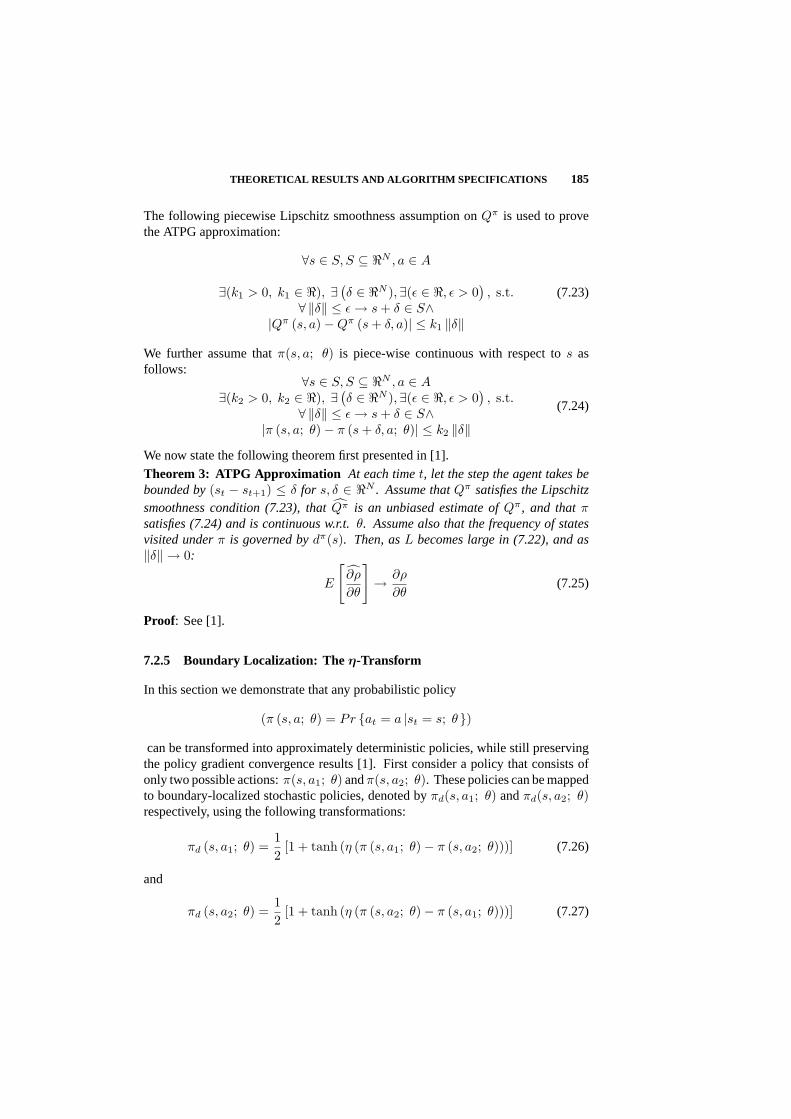
THEORETICAL RESULTS AND ALGORITHM SPECIFICATIONS 185
The following piecewise Lipschitz smoothness assumption onQπ is used to provethe ATPG approximation:
∀s ∈ S, S ⊆ <N , a ∈ A
∃(k1 > 0, k1 ∈ <), ∃ (δ ∈ <N ), ∃(ε ∈ <, ε > 0
), s.t.
∀ ‖δ‖ ≤ ε → s + δ ∈ S∧|Qπ (s, a)−Qπ (s + δ, a)| ≤ k1 ‖δ‖
(7.23)
We further assume thatπ(s, a; θ) is piece-wise continuous with respect tos asfollows:
∀s ∈ S, S ⊆ <N , a ∈ A∃(k2 > 0, k2 ∈ <), ∃ (
δ ∈ <N ), ∃(ε ∈ <, ε > 0), s.t.
∀ ‖δ‖ ≤ ε → s + δ ∈ S∧|π (s, a; θ)− π (s + δ, a; θ)| ≤ k2 ‖δ‖
(7.24)
We now state the following theorem first presented in [1].
Theorem 3: ATPG Approximation At each timet, let the step the agent takes bebounded by(st − st+1) ≤ δ for s, δ ∈ <N . Assume thatQπ satisfies the Lipschitzsmoothness condition (7.23), thatQπ is an unbiased estimate ofQπ, and thatπsatisfies (7.24) and is continuous w.r.t.θ. Assume also that the frequency of statesvisited underπ is governed bydπ(s). Then, asL becomes large in (7.22), and as‖δ‖ → 0:
E
[∂ρ
∂θ
]→ ∂ρ
∂θ(7.25)
Proof: See [1].
7.2.5 Boundary Localization: Theη-Transform
In this section we demonstrate that any probabilistic policy
(π (s, a; θ) = Pr at = a |st = s; θ)
can be transformed into approximately deterministic policies, while still preservingthe policy gradient convergence results [1]. First consider a policy that consists ofonly two possible actions:π(s, a1; θ) andπ(s, a2; θ). These policies can be mappedto boundary-localized stochastic policies, denoted byπd(s, a1; θ) andπd(s, a2; θ)respectively, using the following transformations:
πd (s, a1; θ) =12
[1 + tanh (η (π (s, a1; θ)− π (s, a2; θ)))] (7.26)
and
πd (s, a2; θ) =12
[1 + tanh (η (π (s, a2; θ)− π (s, a1; θ)))] (7.27)
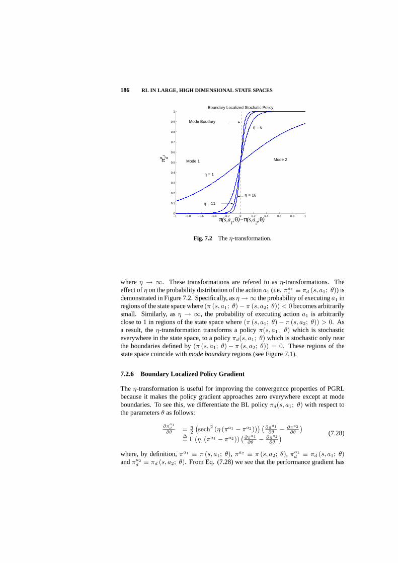
186 RL IN LARGE, HIGH DIMENSIONAL STATE SPACES
−1 −0.8 −0.6 −0.4 −0.2 0 0.2 0.4 0.6 0.8 10
0.1
0.2
0.3
0.4
0.5
0.6
0.7
0.8
0.9
1
π(s,a1;θ)−π(s,a
2;θ)
π da 1
Boundary Localized Stochatic Policy
η = 1
η = 6
η = 11
η = 16
Mode Boudary
Mode 1 Mode 2
Fig. 7.2 Theη-transformation.
whereη → ∞. These transformations are refered to asη-transformations. Theeffect ofη on the probability distribution of the actiona1 (i.e. πa1
c ≡ πd (s, a1; θ)) isdemonstrated in Figure 7.2. Specifically, asη →∞ the probability of executinga1 inregions of the state space where(π (s, a1; θ)− π (s, a2; θ)) < 0 becomes arbitrarilysmall. Similarly, asη → ∞, the probability of executing actiona1 is arbitrarilyclose to 1 in regions of the state space where(π (s, a1; θ)− π (s, a2; θ)) > 0. Asa result, theη-transformation transforms a policyπ(s, a1; θ) which is stochasticeverywhere in the state space, to a policyπd(s, a1; θ) which is stochastic only nearthe boundaries defined by(π (s, a1; θ)− π (s, a2; θ)) = 0. These regions of thestate space coincide withmode boundaryregions (see Figure 7.1).
7.2.6 Boundary Localized Policy Gradient
The η-transformation is useful for improving the convergence properties of PGRLbecause it makes the policy gradient approaches zero everywhere except at modeboundaries. To see this, we differentiate the BL policyπd(s, a1; θ) with respect tothe parametersθ as follows:
∂πa1d
∂θ = η2
(sech2 (η (πa1 − πa2))
) (∂πa1
∂θ − ∂πa2
∂θ
)∆= Γ (η, (πa1 − πa2))
(∂πa1
∂θ − ∂πa2
∂θ
) (7.28)
where, by definition,πa1 ≡ π (s, a1; θ), πa2 ≡ π (s, a2; θ), πa1d ≡ πd (s, a1; θ)
andπa2d ≡ πd (s, a2; θ). From Eq. (7.28) we see that the performance gradient has

THEORETICAL RESULTS AND ALGORITHM SPECIFICATIONS 187
−1 −0.8 −0.6 −0.4 −0.2 0 0.2 0.4 0.6 0.8 10
0.1
0.2
0.3
0.4
0.5
0.6
0.7
0.8
0.9
1
π(s,a1;θ)−π(s,a
2;θ)
ΓBoundary Localized Stochatic Search
Mode 1 Mode 2
Mode Boundary
η = 1
η = 6 η = 11
η = 16
Fig. 7.3 The magnitude of the policy gradient goes to zero everywhere except mode bound-aries asη →∞.
the following proportionality property:∣∣∣∣∂ρ
∂θ
∣∣∣∣ ∝ Γ (η, (πa1 − πa2)) (7.29)
This equation is plotted in Figure 7.3, where we see that asη → ∞, the policygradient approaches zero everywhere except near mode boundaries. As a result, onlyregions in state space near mode boundaries need be stochastically searched when theagent uses BL policies (i.e. mode switching controllers). The direct result of this isthat mode switching policies have a significantly reduced search space for learning,making them particularly suitable for high dimensional RL problems.
It is easy to extend the argument presented above for a policy of two actions (ormodes), to polices that have any finite number of actions (or modes). Thereforethe η-transformation is valid for any finite set of policies, and one can transformany stochastic policy to a BL policy. Next we state theBoundary Localized PolicyGradient Theorem(first stated in [1]), which is a direct extension of the PolicyGradient theorem.
Theorem 4: Boundary Localized Policy Gradient For any MDP, in either theaverage or discounted start-state formulations,
∂ρ
∂θ=
∑s
dπ (s)∑
a
∂πd(s, a; θ)∂θ
Qπ(s, a) (7.30)

188 RL IN LARGE, HIGH DIMENSIONAL STATE SPACES
0 20 40 60 80 100−0.1
0
0.1
0.2
0.3
0.4
0.5
0.6
Number of Policy Updates
ρ(π)
Biased Q No Bias
Linear FA Q
a) Convergence ofAlgorithms
0 2 4 6 8 10 12 1410
0
101
102
103
104
Number of Possible Actions (M)
V[∂
ρ /
∂ θ F
] / V
[∂ ρ
/ ∂
θ]
b) V [ ∂ρ∂θ F
]/V [ ∂ρ∂θ ]
0 2 4 6 8 10 12 1410
0
101
102
Number of Possible Actions (M)
V[∂
ρ /
∂ θ]
/ V
[∂ ρ
/ ∂
θ b]
c) V [ ∂ρ∂θ ]/V [ ∂ρ
∂θ b]
Fig. 7.4 Simulation Results
Proof Sketch: If ∂π/∂θ exists then because theη-transformation is continuouslydifferentiable, so does∂πd/∂θ. The rest of the proof follows that of [5].
The significance of the BLPG theorem is that locally optimal mode switching policescan be learned using policy gradients. As a result, even though search is localizedto a very small region of the state space, a policy gradient algorithm (7.30) will stillconverge to a locally optimum policy.
7.3 EXPERIMENTAL RESULTS
7.3.1 Verification of the Rate of Convergence Results
The Simulated Environment: The experiments simulate an agent episodicallyinteracting in a continuous two dimensional environment. The agent starts eachepisode in the same statesi, and executes a finite number of steps following a policyto a fixed goal statesG. The stochastic policy is defined by a finite set of Gaussians,each associated with a specific action. The Gaussian associated with actionam isdefined as:
gm (s) = exp
[−
D∑
d=1
(sd − cmd)2
vmd
]

EXPERIMENTAL RESULTS 189
wheres = (s1, ..., sD) ∈ <D, is the agents state,cm1, ..., cmD is the Gaussian center,andvm1, ..., vmD is the variance along each state space dimension. The probabilityof executing actionam in states is
π (s, am; θ) =gm (s)
M∑j=1
gj (s)
where θ = (c11, ..., c1d, v11, ..., v1d, ..., cM1, ..., cMD, vM1, ..., vMD) defines thepolicy parameters that dictate the agent’s actions. Actiona1 directs the agent to-ward the goals statesG, while the remaining actionsam (for m = 2, ..., M ) directthe agent towards the corresponding Gaussian centercm1, ..., cmD.
Noise is modeled using a uniform random distribution between(0, 1) denoted byU(0, 1), such that the noise in dimensionsd is given by:
sobsd = sd + δ (U (0, 1)− 0.5)
whereδ > 0 is the magnitude of the noise,sobsd is the state the agent observes and
uses to choose actions, andsd is the actual state of the agent.
The agent receives a reward of +1 when it reaches the goal state, otherwise it receivesa reward of:
r (s) = −0.01 exp
[−
D∑
d=1
s2d
4
]
Thus the agent gets negative rewards the closer it gets to the origin of the state space,and a positive reward whenever it reaches the goal state.
For further details we refer the reader towww.cis.upenn.edu/∼grudic/PGRLSimfor source code and details.
Implementation Details: We sampleQπobs (s, ai) by executing actionai in states
and thereafter following the policy. For the episodic formulation, where the agentexecutes a maximum ofT steps during each episode, at the end of each episode,Qπ
obs (st, at) for stept is evaluated using the following:
Qπobs (st, at) =
∞∑
k=1
γk−1rt+k|st = s, at = a, π
Given that the agent executes a complete episode((s1, a1), ..., (sT , aT )) follow-ing the policy π, at the completion of the episode we can therefore calculate(Qπ
obs(s1, a1), ..., Qπobs(sT , aT )) using the obove equation. This gives direct samples
of T state action value pairs. From (7.5) we require a total ofMT state action valuefunction observations to estimate a performance gradient (forM possible actions).We obtain the remaining(M − 1)T observations ofQπ
obs by sending the agent outon (M − 1)T episodes, each time allowing it to follow the policyπ for all T steps,with the exception that actionat = am is executed whenQπ
obs(st, am) is being
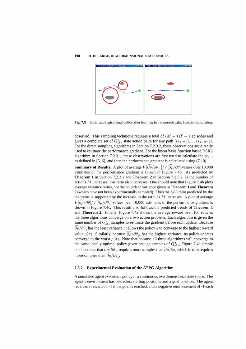
190 RL IN LARGE, HIGH DIMENSIONAL STATE SPACES
Fig. 7.5 Initial and typical final policy after learning in the smooth value function simulation.
observed. This sampling technique requires a total of(M − 1)T − 1 episodes andgives a complete set ofQπ
obs state action pairs for any path((s1, a1), ..., (sT , aT )).For the direct sampling algorithms in Section 7.2.3.2, these observations are directlyused to estimate the performance gradient. For the linear basis function based PGRLalgorithm in Section 7.2.3.1, these observations are first used to calculate thewai,l
as defined in [5, 6], and then the performance gradient is calculated using (7.10).
Summary of Results:A plot of averageV [∂ρ/∂θF ]/V [∂ρ/∂θ] values over 10,000estimates of the performance gradient is shown in Figure 7.4b. As predicted byTheorem 1 in Section 7.2.3.1 andTheorem 2 in Section 7.2.3.2, as the number ofactionsM increases, this ratio also increases. One should note that Figure 7.4b plotsaverage variance ratios, not the bounds in variance given inTheorem 1andTheorem2 (which have not been experimentally sampled). Thus theML ratio predicted by thetheorems is supported by the increase in the ratio asM increases. A plot of averageV [∂ρ/∂θ]/V [∂ρ/∂θb] values over 10,000 estimates of the performance gradient isshown in Figure 7.4c. This result also follows the predicted trends ofTheorem 1andTheorem 2. Finally, Figure 7.4a shows the average reward over 100 runs asthe three algorithms converge on a two action problem. Each algorithm is given thesame number ofQπ
obs samples to estimate the gradient before each update. Because
∂ρ/∂θb has the least variance, it allows the policyπ to converge to the highest reward
valueρ(π). Similarly, because∂ρ/∂θF has the highest variance, its policy updatesconverge to the worstρ(π). Note that because all three algorithms will converge tothe same locally optimal policy given enough samples ofQπ
obs, Figure 7.4a simply
demonstrates that∂ρ/∂θF requires more samples than∂ρ/∂θ, which in turn requires
more samples than∂ρ/∂θb.
7.3.2 Experimental Evaluation of the ATPG Algorithm
A simulated agent executes a policy in a continuous two dimensional state space. Theagent’s environment has obstacles, starting positions and a goal position. The agentreceives a reward of +1 if the goal is reached, and a negative reinforcement of -1 each

EXPERIMENTAL RESULTS 191
time it hits an obstacle. The learning objective is to modify the policy (modelledby a set of Guassians as defined below) such that it avoids hitting obstacles whileminimizing the time it takes to reach the goal. The agent uses a discount rewardformulation.
The agent can execute one of two types of actions: move away from the center ofa Gaussian or move towards the center of a Gaussian. Therefore the total numberof actions is defined by the number of Gaussians in the agent’s policy. There arefour parameters per Gaussian: two defining its position(X,Y ) in the 2 dimensionalstate space, and two defining its width(Sx, Sy) (these make up theθ parameters inthe policyπ(s, a; θ)). The agent chooses actions stochastically at each location inthe state space, with the probability of executing an action being proportional to therelative magnitude of each Gaussian.
Typical paths followed by the agent are shown in Figure 7.5. The figure shows pathsfollowed by the agent before and after learning as it moves along the dotted line froma starting point on the left hand side to the goal (small circle) on the right, whileavoiding the obstacles (shaded ellipsoid region). The agent’s policy in Figure 7.5 isdefined by three Gaussians, resulting inθ being a 12-dimensional vector that defineπ(s, a; θ). The location and width of two of the Gaussians is symbolized by regionsenclosed by elliptical curves surrounding the shaded obstacles, which represent areasof the state space where the action associated with the Gaussian has the greatestprobability of being executed. The ellipses symbolize the “move away from” theGaussian center actions. The final Gaussian is centered at the goal position (the farright lightly shaded circle) and represents the “move towards” Gaussian center (i.e.goal position) action. The “move towards” goal action is most probably everywhereexcept within the black ellipse regions.
We compare the ATPG, PIFA and REINFORCE algorithms (see [2] for algorithmimplementation details) on two types of simulated environments: one shown in Figure7.5 which has a continuous value function with respect to changes in the policy (i.e.the functionQπ(s, a) changes smoothly as the parametersθ of the policy change),and one shown in Figure 7.6 which has a discontinuous value function with respectto changes in the policy.
7.3.2.1 Smooth Value Function Simulation The initial and learned policies ofan agent in an environment where it never collides with an obstacle are shown inFigure 7.5. As learning progresses and the policyπ(s, a; θ) is changed, the valuefunctionQπ(s, a) changes continuously with respect toθ. The left graphic in Figure7.5 shows a typical path given an initial policy specification, and the right graphic inFigure 7.5 shows a typical path taken under the learned policy after either the ATPGor PIFA algorithms have converged. Both algorithms converge to a policy whichtakes the agent from the initial position to the final position in the shortest number ofsteps.
The ATPG and PIFA algorithms were compared forL = 1, 3, 5, 7, and10. Theaverage number of episodes over ten runs for the ATPG algorithm to converge rangedfrom 120 (standard deviation 10) forL = 1, to 1300 (standard deviation 150) for
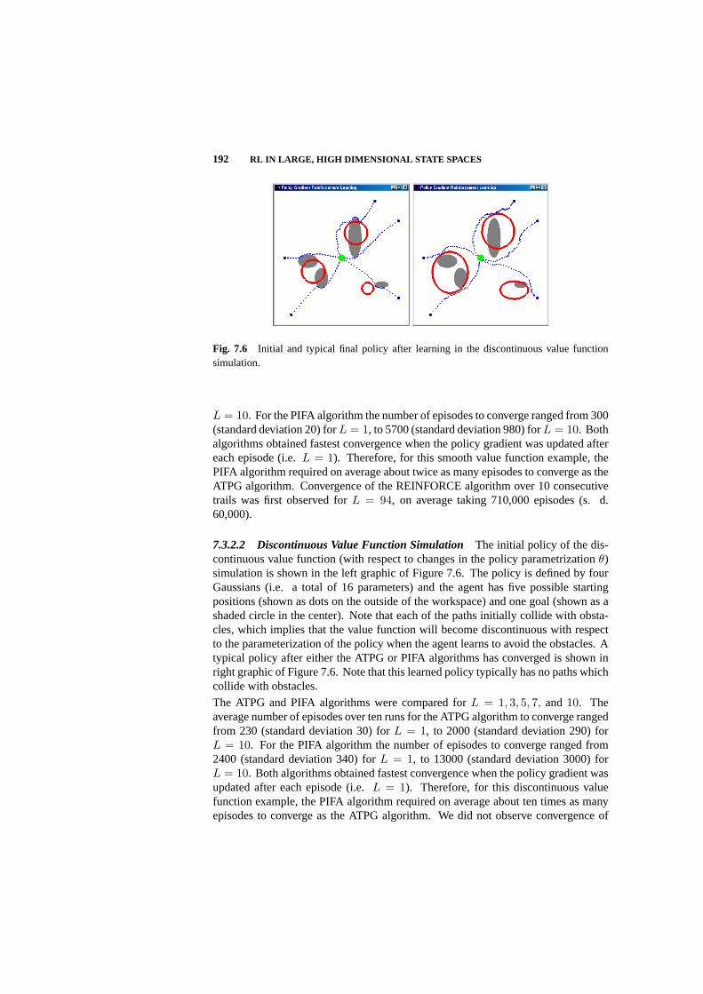
192 RL IN LARGE, HIGH DIMENSIONAL STATE SPACES
Fig. 7.6 Initial and typical final policy after learning in the discontinuous value functionsimulation.
L = 10. For the PIFA algorithm the number of episodes to converge ranged from 300(standard deviation 20) forL = 1, to 5700 (standard deviation 980) forL = 10. Bothalgorithms obtained fastest convergence when the policy gradient was updated aftereach episode (i.e.L = 1). Therefore, for this smooth value function example, thePIFA algorithm required on average about twice as many episodes to converge as theATPG algorithm. Convergence of the REINFORCE algorithm over 10 consecutivetrails was first observed forL = 94, on average taking 710,000 episodes (s. d.60,000).
7.3.2.2 Discontinuous Value Function Simulation The initial policy of the dis-continuous value function (with respect to changes in the policy parametrizationθ)simulation is shown in the left graphic of Figure 7.6. The policy is defined by fourGaussians (i.e. a total of 16 parameters) and the agent has five possible startingpositions (shown as dots on the outside of the workspace) and one goal (shown as ashaded circle in the center). Note that each of the paths initially collide with obsta-cles, which implies that the value function will become discontinuous with respectto the parameterization of the policy when the agent learns to avoid the obstacles. Atypical policy after either the ATPG or PIFA algorithms has converged is shown inright graphic of Figure 7.6. Note that this learned policy typically has no paths whichcollide with obstacles.
The ATPG and PIFA algorithms were compared forL = 1, 3, 5, 7, and10. Theaverage number of episodes over ten runs for the ATPG algorithm to converge rangedfrom 230 (standard deviation 30) forL = 1, to 2000 (standard deviation 290) forL = 10. For the PIFA algorithm the number of episodes to converge ranged from2400 (standard deviation 340) forL = 1, to 13000 (standard deviation 3000) forL = 10. Both algorithms obtained fastest convergence when the policy gradient wasupdated after each episode (i.e.L = 1). Therefore, for this discontinuous valuefunction example, the PIFA algorithm required on average about ten times as manyepisodes to converge as the ATPG algorithm. We did not observe convergence of
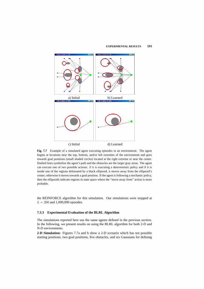
EXPERIMENTAL RESULTS 193
a) Initial
b) Learned
c) Initial
d) Learned
Fig. 7.7 Example of a simulated agent executing episodes in an environment. The agentbegins at locations near the top, bottom, and/or left extremes of the environment and goestowards goal positions (small shaded circles) located at the right extreme or near the center.Dashed lines symbolize the agent’s path and the obstacles are the larger gray areas. The agentcan execute one of two possible actions: if it is executing a deterministic policy and if it isinside one of the regions delineated by a black ellipsoid, it moves away from the ellipsoid’scenter; otherwise it moves towards a goal position. If the agent is following a stochastic policy,then the ellipsoids indicate regions in state space where the “move away from” action is moreprobable.
the REINFORCE algorithm for this simulation. Our simulations were stopped atL = 200 and 1,000,000 episodes.
7.3.3 Experimental Evaluation of the BLRL Algorithm
The simulations reported here use the same agents defined in the previous section.In the following, we present results on using the BLRL algorithm for both 2-D andN-D environments.
2-D Simulation: Figures 7.7a and b show a 2-D scenario which has ten possiblestarting positions, two goal positions, five obstacles, and six Gaussians for defining

194 RL IN LARGE, HIGH DIMENSIONAL STATE SPACES
Stochastic Stochastic DeterministicRL BLRL BLRL
Episodes to 6900 600 260converge (sd 400) (sd 90) (sd 40)
Table 7.1 2-D Convergence results with standard deviations.
policies (five for “move away from” which are shown as ellipsoids, and one for “movetowards goal”, which is most probable everywhere except inside the ellipsoids). Thereare a total of 24 policy parametersθ.
Figure 7.7a shows the initial policy and the resulting paths through the environment.Note that four paths end before a goal is reached and eight paths have collisions withobstacles. Figure 7.7b shows the paths after the policy parameters have converged tostable values. The location and extent of the Gaussians has converged such that noneof the paths now collide with obstacles, and the total distance travelled through statespace is shorter than initial policy path.
Table 7.1 shows the average number of episodes (over ten runs) required for conver-gence for the three types of polices studied: stochastic, boundary localized stochastic(η = 16), and deterministic. Note that the purely stochastic polices take the greatestnumber of episodes to converge, while the deterministic policies take the fewest.
N-D Simulation: Our high dimensional simulation include 4, 8, 16, 32, 64, and 128dimensional environments, with the number of policy parametersθ ranging from 14to 512 (i.e. 2 parameters per Gaussian per dimension). The projection of all of theseenvironments into the 2 dimensional XY plane is shown in Figure 7.7c and d. Figure7.7c shows the starting policies, while Figure 7.7d shows policies after convergence.The convergence results are summarized in Figure 7.8 (over ten runs with standarddeviation bars) for the three types of policies studied: stochastic, boundary localizedstochastic (η = 16), and deterministic. For both the deterministic and boundarylocalized policies, convergence is essentially constant with dimension. However, forthe stochastic policy, the convergence times explode with dimension. We only reportconvergence results up to 16 dimensions for stochastic policies - convergence onhigher dimensions was still not achieved after20, 000 iterations, at which time thesimulation was stopped.
7.4 CONCLUSION
The goal of this chapter is to propose a formulation for reinforcement learning thatconverges quickly in very high dimensional state spaces. We argue that the PolicyGradient Reinforcement Learning framework is an effective paradigm for large prob-lem domains, and present theoretical and experimental results to support our position.

CONCLUSION 195
0 20 40 60 80 100 120 1400
500
1000
1500
2000
2500
3000
3500
4000
4500ND Convergence Results
Dimensions
Epi
sode
s to
Con
verg
e Stochastic Policy
Boundary Localize Policy
Deterministic Policy
Fig. 7.8 N-D convergence results over ten runs with standard deviation bars.
Specifically, we show that gradients of increased reward in policy space can be ef-ficiently estimated using the Action Transition Policy Gradient (ATPG) algorithm.In addition, we show that if the agent’s control system (i.e. policy) belongs to thegeneral class of widely used mode switching controllers, then Boundary LocalizedReinforcement Learning (BLRL), can be used to give extremely fast convergence tolocally optimal policies, in very high dimensional state spaces.
Acknowledgments
Thanks to Vijay Kumar and Jane Mulligan for discussing this work with us. This work wasfunded by the IRCS at the University of Pennsylvania, and by the DARPA ITO MARS grantno. DABT63-99-1-0017.

Bibliography
1. G. Z. Grudic and L. H. Ungar Localizing Search in Reinforcement Learning. InProceedings of the Seventeenth National Conference on Artificial Intelligence,volume 17, pp: 590-595, 2000.
2. G. Z. Grudic and L. H. Ungar Localizing Policy Gradient Estimates to ActionTransitions. InProceedings of the Seventeenth International Conference onMachine Learning, volume 17, pp: 343-350, 2000.
3. G. Z. Grudic and L. H. Ungar Rates of Convergence of Performance GradientEstimates Using Function Approximation and Bias in Reinforcement Learning.In Advances in Neural Information Processing Systems, volume 14, pp: 1515-1522, 2002.
4. L. Baird and A. W. Moore Gradient Descent for General Reinforcement Learning.In Advances in Neural Information Processing Systems, volume 11, 1999.
5. R. S. Sutton, D. McAllester, S. Singh, and Y. Mansour Policy Gradient Methodsfor Reinforcement Learning with Function Approximation. InAdvances inNeural Information Processing Systems, volume 12, 2000.
6. V. R. Konda and J. N. Tsitsiklis Actor-Critic Algorithms. InAdvances in NeuralInformation Processing Systems, volume 12, 2000.
7. J. Baxter and P. L. Bartlett Direct Gradient-Based Reinforcement Learning:I. Gradient Estimation Algorithms. InTechnical Report of Computer SciencesLaboratory, Australian National University, 1999.
8. L. C. Baird Advantage Updating. InTechnical Report of Wright-Patterson AirForce Base, 1993.
9. L. C. Baird Residual algorithms: reinforcement learning with function approxi-mation. InProceedings of the Twelfth Int. Conf. on Machine Learning, pp: 30-371995.
10. R. S. Sutton Generalization in Reinforcement Learning: Successful ExamplesUsing Sparse Coarse Coding. InAdvances in Neural Information ProcessingSystems, volume 8, pp: 1038–1044, 1996.
196
BIBLIOGRAPHY 197
11. J. A. Boyan and A. W. Moore Generalization in Reinforcement Learning: SafelyApproximating the Value Function. InAdvances in Neural Information Process-ing Systems, volume 7, pp: 369-376, 1995.
12. R. J. Williams Simple statistical gradient-following algorithms for connectionistreinforcement learning. InMachine Learning, volume 8, pp: 229-256, 1992.
13. R. J. Williams A class of gradient-estimating algorithms for reinforcementlearning in neural networks. InProceedings of the IEEE First InternationalConference on Neural Networks, 1987.
14. L. P. Kaelbling and M. L. Littman and A. W. Moore Reinforcement Learning:A Survey. InJournal of Artificial Intelligence Research, volume 4, pp: 237-285,1996.
15. G. J. Gordon Stable Function Approximation in Dynamic Programming. InProceedings of the Twelfth Int. Conf. on Machine Learning, volume 4, pp: 261-268, 1995.
16. John N. Tsitsiklis and Benjamin Van Roy Feature-Based Methods for LargeScale Dynamic Programming. InMachine Learning, volume 22, pp: 59, 1996.
17. D. P. Bertsekas and J. N. Tsitsiklis Neuro-Dynamic Programming. AthenaScientific, 1996.
18. D. G. Lainiotis A Unifying Framework for Adaptive Systems, I: Estimation, II.In Proceedings of the IEEE, volume 64, pp: 1126-1134, 1182-1197, 1976.
19. B. Kuipers and K. J. Astrom The composition and validation of heterogeneouscontrol laws. InAutomatica, volume 30, pp: 233-249, 1994.
20. K. S. Narendra and J. Balakrishnan and K. Ciliz Adaptation and Learning UsingMultiple Models, Switching and Tuning. InIEEE Control Systems Magazine,volume 15, pp: 37-51, 1995.
21. R. S. Sutton and A. G. Barto Reinforcement Learning: An Introductio. MITPress, 1998.
22. R. S. Sutton and D. Precup and S. Singh Between MDPs and semi-MDPs: AFramework for Temporal Abstraction in Reinforcement Learning. InArtificialIntelligence, volume 112, pp: 181-211, 1999.
23. R. Brooks A robust layered control system for a mobile robot. InIEEE Journalof Robotics and Automation, volume 2, pp: 14-23, 1986.
24. M. Kearns and S. Singh Finite-Sample Convergence Rates for Q-Learning andIndirect Algorithms. InAdvances in Neural Information Processing Systems,volume 11, 1999.

198 BIBLIOGRAPHY
25. Marvin Minsky Steps Toward Artificial Intelligence. InComputers and Thought,pp: 406-450, 1963.
26. Jonathan Baxter and Peter L. Bartlett Reinforcement Learning in POMDP’svia Direct Gradient Ascent. InProceedings of the Seventeenth InternationalConference on Machine Learning (ICML’2000), pp: 41-48, 2000.
27. W. H. Press and B. P. Flannery and S. A. Teukolsky and W. T. Vetterling Nu-merical Recipes in C. Cambridge University Press, 1998.
28. R. S. Sutton and A. G. Barto Time-derivative models of pavlovian reinforce-ment. InLearning and Computational Neuroscience: Foundations of AdaptiveNetworks, pp: 497-537, 1990.
29. Leonid Peshkin and Kee-Eung Kim and Nicolas Meuleau and Leslie Pack Kael-bling Learning to Cooperate via Policy Search. InProceedings of the SixteenthInternational Conference on Uncertainty in Artificial Intelligence (UAI 2000),2000.
30. R. Fierro and A. Das and J. Spletzer and Y. Hur and R. Alur and J. Espositoand G. Grudic and V. Kumar and I. Lee and J. P. Ostrowski and G. Pappasand J. Southall and C. J. Taylor A framework and architecture for multirobotcoordination. InInternational Journal of Robotics Research, 2003.

8 Hierarchical Decision Making
MALCOLM RYAN
University of New South Wales
Editor’s Summary: As the field of reinforcement learning has advanced, interest insolving realistic control problems has increased. However, Markov Decision Process(MDP) models have not proven sufficient to the task. This has led to increaseduse of Semi-Markov Decision Process models and the development of HierarchicalReinforcement Learning (HRL). This chapter is an overview of HRL beginning witha discussion of the problems with the standard MDP models, then presenting thetheory behind HRL, and finishing with some actual HRL algorithms that have beenproposed. To see some examples of how hierarchical methods perform, see Chapter11.
8.1 INTRODUCTION
Reinforcement learning [49, 24] is a field of machine learning dedicated to buildingalgorithms which learn to control the interaction of an agent with an environment,to achieve particular goals. For over a decade, since the advent of TD(λ) [46] andQ-Learning [54], most of the work in reinforcement learning has been based onthe Markov Decision Process (MDP) model. While these algorithms have strongtheoretical convergence properties, they have often performed poorly in practice.Optimal policies can be found for simple toy problems, but the algorithms are oftendifficult to scale up to realistic control problems.
Part of the problem is that MDPs model a system in fine detail. In recent years therehas been a move from Markov Decision Processes to Semi-Markov Decision Pro-cesses, in an attempt to build models at higher levels of abstraction. This abstractionprovides a number of advantages which allow us to apply reinforcement learning toa significantly larger collection of problems.
This field is known as Hierarchical Reinforcement Learning (HRL) and has beenthe subject of rapid growth in the past few years. Many techniques have arisen, allbased on similar foundations but taking them in different directions. This profusion of
199

200 HIERARCHICAL DECISION MAKING
different approaches can hide both the commonalities shared by these algorithms, andthe different orthogonal improvements each approach contains. Many approachescombine several improvements into a single algorithm, which need not intrinsicallybe tied together.
In order to clarify this situation, we divide this review into three sections. In thefirst section we outline the problems with the standard MDP model for reinforcementlearning in greater detail. In the second section we present the theory behind Hier-archical Reinforcement Learning and describe some of the different improvementsit can offer. In the third section we describe some of the actual hierarchical rein-forcement learning algorithms which have been published and try to show how theycombine the different elements we have previously described.
This review tries to capture the motivations underlying the movement towards hier-archical reinforcement learning, and some of the prominent examples thereof. It isnot exhaustive. For an alternative presentation, with several recent inventions thatare omitted here, we refer the reader to Barto and Mahadevan’s survey [3].
8.2 REINFORCEMENT LEARNING AND THE CURSE OFDIMENSIONALITY
Reinforcement learning models an agent interacting with an environment, trying tooptimise its choice of action according to some reward criterion. The agent operatesover a sequence of discrete time-steps(t, t + 1, t + 2, . . .). (One time-step indicatesthe duration of a single action. This may or may not correspond to a fixed unit oftime in the real-world.)
At each step the agent observes the state of the environmentst and selects anappropriate actionat. Executing the action produces a change in the state of theenvironment tost+1. It is generally assumed that the sets of possible statesS andavailable actionsA are both finite. This is not always the case in practice, but itgreatly simplifies the theory, so we shall follow this convention.
The mapping of states to actions is done by an internal policyπ. The initial policy isarbitrarily chosen, generally random, and it is modified and improved based on theagent’s experiences. Each experience〈st, at, st+1〉 is evaluated according to somefixed reward function, yielding a rewardrt ∈ <. The agent’s objective is to modifyits policy to maximise its long-term reward. There are several possible definitions of“long-term reward” but the one most commonly employed is theexpected discountedreturngiven by:
Rt = Ert + γrt+1 + γ2rt+2 + . . .
= E
∑∞i=0 γirt+i
(8.1)
whereγ is thediscount ratethat specifies the relative weight of future rewards, with0 ≤ γ < 1. Should the agent reach some terminal statesT , then the infinite sum is cut

REINFORCEMENT LEARNING AND THE CURSE OF DIMENSIONALITY 201
short: all subsequent rewardsrT+1, rT+2, . . . are considered to be zero. (Another,less commonly used, reward criterion isaverage reward[29, 41, 43].)
To ensure that this optimisation problem is well-founded, most reinforcement learningalgorithms place a strong constraint on the structure of the environment. They assumethat it operates as aMarkov Decision Process(MDP) [37]. An MDP describes aprocess that has no hidden state or dependence on history. The outcomes of everyaction, in terms of state transition and reward, obey fixed probability distributionsthat depend only on the current state and the action performed.
Formally an MDP can be described as a tuple〈S,A, T, R〉 whereS is a finite set ofstates,A is a finite set of actions,T : S ×A×S → [0, 1] is a transition function andR : S ×A×< → [0, 1] is a reward function with:
T (s′|s, a) = P (st+1 = s′ | st = s, at = a) (8.2)
R (r|s, a) = P (rt = r | st = s, at = a) (8.3)
which respectively express the probability of ending up in states′ and receivingrewardr after executing actiona in states. These probabilities must be independentof any criteria other than the values ofs anda. This is called theMarkov Property.An in-depth treatment of the theory of Markov Decision Processes can be found inany of [5, 6, 7, 19, 37, 49].
Given this simplifying assumption, the best action to choose in any state dependson that state alone. This means that the agent’s policy can be expressed as a purelyreactive mapping of states to actions,π : S → A. Furthermore every states can beassigned a valueV π(s) that denotes the expected discounted return if the policyπ isfollowed:
V π(s) = E Rt | ε(π, s, t) (8.4)
= E
∞∑
i=0
γirt+i | ε(π, s, t)
(8.5)
=∫ +∞
−∞rRrs, adr + γ
∑
s′∈STs′s, aV π(s′) (8.6)
whereε(π, s, t) denotes the event of policyπ being initiated in states at timet. V π
called thestate value functionfor policy π.
An optimal policycan now be simply defined as a policyπ? that maximisesV π(s)for all statess. The Markov property guarantees that there is such a globally optimalpolicy [49] although it may not be unique. We define theoptimal state-value functionV ?(s) as being the state value function of the policyπ?:
V ?(s) = V π?
(s)= maxπ V π(s)
(8.7)

202 HIERARCHICAL DECISION MAKING
We can also define anoptimal state-action value functionQ?(s, a) in terms ofV ?(s)as:
Q?(s, a) = E rt + γV ?(st+1) | st = s, at = a (8.8)
This function expresses the expected discounted return if actiona is executed in states and an optimal policy is followed thereafter. If such a function is known then anoptimal policy can be extracted from it simply:
π?(s) = arg maxa∈A
Q?(s, a) (8.9)
Thus the reinforcement learning problem can be transformed from learning an optimalpolicy π? to learning the optimal state-action value functionQ?. 1 This turns outto be a relatively straightforward dynamic programming problem, which could inprinciple be solved by conventional DP algorithms.
There is, however, one complication. Standard techniques such as value-iteration orpolicy-iteration [5] rely on us already having an accurate model of the underlyingMDP. However, in reinforcement learning we assume that this model is not (initially)available. Our only source of information about the MDP is experimental interactionwith the environment. Given this we can proceed in two ways: we can attempt tolearn a model and then applied standard DP methods to construct a policy, or wecan attempt to learnQ? directly. These are called “model-based” and “model-free”approaches respectively. Much work has been done in both these areas, but model-free approaches tend to dominate. We perpetuate this bias in this chapter, focusing onmodel-free reinforcement learning, which is where most of the work in hierarchicallearning has been taking place. We briefly summarise some of the model-basedhierarchical learning towards the end of the chapter.
8.2.1 Q-Learning
Q-Learning[54] is widely regarded as the archetypal model-free reinforcement learn-ing algorithm. It is an online incremental learning algorithm that learns anapprox-imate state-action value functionQ(s, a) that converges to the optimal functionQ?
in Eq. 8.8 above (under certain conditions outlined below). It is a simple algorithmwhich avoids the complexities of modelling the functionsR and T of the MDPby learningQ directly from its experiences. It has significant practical limitations,but is theoretically sound and has provided a foundation for many more complexalgorithms. Pseudocode for this algorithm is given in Algorithm 1.
The approximate Q-function is stored in a table. Its initial values may be arbitrarilychosen, typically they are all zero or else randomly assigned. At each time-step an
1In practice it is only necessary for the agent to optimise its reward in the states it actually encounters.Complete optimal policies are not needed to do this as some states may never be reached. This is one wayin which reinforcement learning differs from classical MDP solution methods.
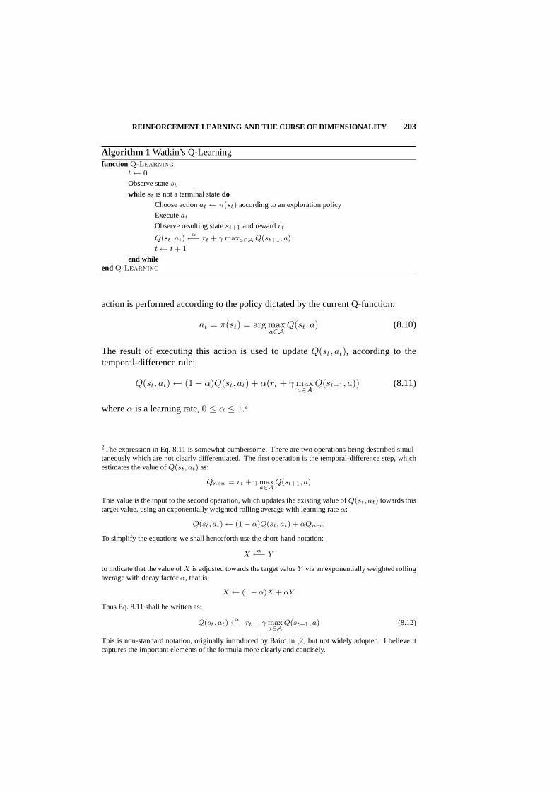
REINFORCEMENT LEARNING AND THE CURSE OF DIMENSIONALITY 203
Algorithm 1 Watkin’s Q-Learningfunction Q-Learning
t ← 0
Observe statest
while st is not a terminal statedoChoose actionat ← π(st) according to an exploration policy
Executeat
Observe resulting statest+1 and rewardrt
Q(st, at)α←− rt + γ maxa∈AQ(st+1, a)
t ← t + 1
end whileendQ-Learning
action is performed according to the policy dictated by the current Q-function:
at = π(st) = arg maxa∈A
Q(st, a) (8.10)
The result of executing this action is used to updateQ(st, at), according to thetemporal-difference rule:
Q(st, at) ← (1− α)Q(st, at) + α(rt + γ maxa∈A
Q(st+1, a)) (8.11)
whereα is a learning rate,0 ≤ α ≤ 1.2
2The expression in Eq. 8.11 is somewhat cumbersome. There are two operations being described simul-taneously which are not clearly differentiated. The first operation is the temporal-difference step, whichestimates the value ofQ(st, at) as:
Qnew = rt + γ maxa∈A
Q(st+1, a)
This value is the input to the second operation, which updates the existing value ofQ(st, at) towards thistarget value, using an exponentially weighted rolling average with learning rateα:
Q(st, at) ← (1− α)Q(st, at) + αQnew
To simplify the equations we shall henceforth use the short-hand notation:
Xα←− Y
to indicate that the value ofX is adjusted towards the target valueY via an exponentially weighted rollingaverage with decay factorα, that is:
X ← (1− α)X + αY
Thus Eq. 8.11 shall be written as:
Q(st, at)α←− rt + γ max
a∈AQ(st+1, a) (8.12)
This is non-standard notation, originally introduced by Baird in [2] but not widely adopted. I believe itcaptures the important elements of the formula more clearly and concisely.
204 HIERARCHICAL DECISION MAKING
The approximate state-action value functionQ is proven to converge to the optimalfunctionQ? (and henceπ to π?) given certain technical restrictions on learning rates(∑∞
t=1 αt = ∞ and∑∞
t=1 α2t < ∞) and the requirement that all state-action pairs
continue to be updated indefinitely [55, 53, 22]. This second requirement meansthat in executing the learnt policy the agent must also do a certain proportion ofnon-policy actions for the purposes of exploration. Exploration is important in allthe algorithms that follow. The simplest approach to exploration is theε-greedyalgorithm which simply takes an exploratory action with some small probabilityε,and a policy action otherwise. A large number of more complex alternatives exist(see [52] for a summary).
8.2.2 The curse of dimensionality
As stated above, Q-Learning is theoretically guaranteed to converge to an optimalpolicy, however the guarantee is only true in the limit, and in practical problems ofany significant size it has often been found to be impracticably slow. Without doinga full analysis of the algorithm, we can observe certain factors which contribute tothis failure.
To find an optimal policy, a Q-value must be learnt for every state-action pair. Thismeans, first of all, that every such pair needs to be explored at least once. Soconvergence time is at bestO(|S|.|A|). Real-world problems typically have largemulti-dimensional state spaces.|S| is exponential in the number of dimensions, soeach extra dimension added to a problem multiplies the time it takes.
Furthermore, states are generally only accessible from a handful of close neighbours,so the distance between any pair of states in terms of action steps also increaseswith the size and dimensionality of the space. Yet a change in the value of one statemay have consequences for the policy in a far distant state. As information can onlypropagate from one state to another through individual state transitions, the furtherapart two states are, the longer it will take for this information to be propagated. Thusthe diameter of the state space is an additional factor in the time required to reachconvergence.
A general-purpose solution to this problem has not yet been found. There have beenmany attempts to represent the table of Q-values more compactly by using one varietyof function approximator or another. These have met with mixed success. Sometimesthe resulting state-abstraction has enabled the learning algorithm to learn an effective(not necessarily optimal) policy in times faster than without abstraction by an orderof magnitude or more for a particular domain (eg. [51, 56, 4]), but no such approachhas proven to be a general-purpose solution. What works well in one domain will failspectacularly in another. Furthermore even the simplest and most conservative formsof function approximation have been shown to break the convergence proofs, causingQ-values to becoming wildly divergent in certain situations [2]. For a summary ofsuch attempts, see [24].
As a result of these difficulties researchers have turned from seeking general-purposeto special-purpose solutions. It has been recognised that a number of the most

HIERARCHICAL REINFORCEMENT LEARNING IN THEORY 205
successful applications of reinforcement learning have used significant task-specificbackground knowledge tacitly incorporated into the agent’s representation of its statesand actions. Focus is shifting towards creating an architecture by which this tacitinformation can become explicit and can be represented in a systematic way. The aimis to create systems that can benefit from the programmer’s task-specific knowledgewhilst maintaining desirable theoretical properties of convergence.
8.3 HIERARCHICAL REINFORCEMENT LEARNING IN THEORY
Significant attention has recently been given to hierarchical decomposition as a meansto this end. “Hierarchical reinforcement learning” (HRL) is the name given to a classof learning algorithms that share a common approach to scaling up reinforcementlearning.
Hierarchical decomposition has always been a natural approach to problem solving.“Divide-and-conquer” has long been a familiar motto in computer science. A complexproblem can often be solved by decomposing it into a collection of smaller problems.The smaller problems can be solved more easily in isolation, and then recombinedinto a solution for the whole. Inspiration for hierarchical reinforcement learningcame partly from behaviour-based techniques for robot programming [10, 28, 31]and partly from the hierarchical methods used in symbolic planning [40, 26, 21, 25].
Hierarchical reinforcement learning accelerates learning by forcing a structure onthe policies being learnt. The reactive state-to-action mapping of Q-learning isreplaced by a hierarchy of temporally-abstract actions. These are actions that operateover several time-steps. Like a subroutine or procedure call, once a temporallyabstract action is executed it continues to control the agent until it terminates, atwhich point control is restored to the main policy. These actions (variously calledsubtasks, behaviours, macros, options, activitiesor abstract machinesdepending onthe particular algorithm in question) must themselves be further decomposed intoone-step actions that the agent can execute. We shall henceforth refer to one-stepactions asprimitive actionsand temporally-abstract actions asbehaviours. Policieslearnt using primitive actions alone shall be calledmonolithic to distinguish themfrom hierarchicalor behaviour-basedpolicies.
How does this decomposition aid us? There are two different ways. One, it allowsus to limit the choices available to the agent, even to the point of hard-coding partsof the policy; and two, it allows us to specify local goals for certain parts of thepolicy. Different HRL algorithms implement these features in different ways. Someimplement one and not the other. We shall postpone describing specific algorithmsuntil Section 8.4, and for the moment present these features in more general terms,with the aid of an example.

206 HIERARCHICAL DECISION MAKING
Bathroom Bedroom2
Study LoungeCloset
Robot
Coffee Book
Hall
Laundry
Dining
KitchenBedroom1
Fig. 8.1 An example environment.
8.3.1 A Motivating Example
Figure 8.1 shows an example environment we shall use to illustrate the concepts inthis chapter. Imagine that the learning agent is a house-hold robot in a house with thelayout shown. Its purpose is to fetch objects from one room to another. It is able toknow its location with a precision as shown by the cells of the grid, and its primitiveactions enable it to navigate from a cell to any of its eight neighbours, with a smallprobability of error.
If the robot is in the same cell as an object, it can pick it up and carry it. Thereare two objects in the environment that we are interested in. In the kitchen in thenorth-west corner of the map is a machine which dispenses a cup of coffee. In thesecond bedroom there is a book, also indicated on the map. The robot starts at itsdocking location in the study. Its goal will vary from example to example as weconsider different aspects of HRL (and later, of planning).
In this environment we have 15,000 states (75 × 50 cells, with two different statesfor each object, depending on whether the robot is holding it or not3) and 9 primitiveactions (each of the 8 compass directions, plus the pickup action). This is not in itselfa complex environment, and most goals will be relatively easy to complete, but it iscertainly one that can be made simpler by providing an appropriate set of behaviours.
3The positions of the book and the coffee machine in their respective rooms are also part of the state butsince these positions are fixed, and the robot cannot drop these objects elsewhere, this information can beomitted.
HIERARCHICAL REINFORCEMENT LEARNING IN THEORY 207
The obvious behaviours to specify are:Go(Room1, Room2) which moves the robotbetween two neighbouring rooms, andGet(Object, Room) which moves towards andpicks up the specified object when the robot is in the same room as it. We will discusshow these behaviours are implemented as we examine individual techniques.
8.3.2 Limiting the Agent’s Choices
Since learning time is dominated by the number of state-action pairs that need to beexplored, the obvious way to accelerate the process is to cut down the number of suchpairs. Using background knowledge we can identify action choices which are plainlyunhelpful and eliminate them from the set of possible policies. There is a variety ofways in which this can be done. Of course, such limitations must be applied withcare, as overly broad limitations can prevent the agent from discovering policies thatmight otherwise be optimal.
Limiting Available Primitive Actions The simplest solution is to hard-code portionsof the policy. Some or all of the internal operation of a behaviour can be written byhand by the system designer. This removes the need for the agent to do any kindof learning at all for significant portions of the state space, which will immediatelyimprove performance. This assumes however that the system designer is able to dothis. Part of the point of learning policies is to relieve the designer of the need tospecify them, so this may be of limited use. Still, there are some situations in whichsimple behaviours might be wholly or partially specified, and algorithms have beendesigned to take advantage of this.
Less drastically, the internal policy of a behaviour could be learnt using only a limitedsubset of all available primitive actions. This is useful if the system designer knowsthat certain primitive actions are only suitable for particular behaviours and not forothers. From the example, theGo() behaviours could reasonably be limited to onlyuse the primitive actions which move the robot, and ignore the pickup action, whichwould be of no use to that behaviour.
Note that it is not strictly necessary to use hierarchy to limit primitive action choice.A simple extension to the MDP formalism above would allow the admissible actionset to be a function of the state. The Q-Learning algorithm can be successfullyapplied to this problem with only a slight modification. However adding hierarchyallows us to specify these restrictions on the wider context of the subtask we currentlyexecuting, as well as the immediate state.
Limiting Available Behaviours Likewise, limits can be placed on which behavioursare available to the agent at different times. Behaviours are generally limited in scope,so they often can only be executed from a subset of all possible states. For instancetheGet() behaviour can only be applied when the agent is it the same room as thetarget object. The set of states in which a behaviourB can be applied is called itsapplicability space, which we shall denoteB.pre. Learning algorithms should notallow the agent to choose a behaviour in a state in which it is not applicable.

208 HIERARCHICAL DECISION MAKING
However this may not be limiting enough. As more ambitious problems are tackled,the repertoire of behaviours available to an agent is likely to become large, and manybehaviours will have overlapping applicability spaces. It is of no use to limit theinternal policy choices of behaviours if choosing between the behaviours becomesjust as difficult.
To this end, most HRL algorithms implement some kind oftask hierarchytolimit the choice of behaviours to those that are appropriate to the agent’s situ-ation. Consider the situation in the example environment when the robot is inhall with the goal of fetching both the book and the coffee. There are six ap-plicable behaviours:Go(hall, study), Go(hall, dining), Go(hall, bedroom1),Go(hall, bathroom), Go(hall, bedroom2), andGo(hall, lounge). Of these, onlytwo are appropriate:Go(hall, dining), if the agent decides to fetch the coffee first,andGo(hall, bedroom2) if the agent decides to fetch the book. Exploring the othersis a waste of time. The system designer, who specified the behaviours, should realisethis and incorporate it into the task hierarchy, limiting the agent’s choices in this sit-uation to one of these two behaviours. The larger an agent’s repertoire of behavioursbecomes, the more critical this kind of background knowledge.
Committing to Behaviours Finally, choices are limited by requiring long-termcommitmentto a behaviour. It is conceivable that a learning algorithm could bewritten which implemented hard-coded behaviours but allowed the agent to choosea different behaviour on every time step. Such an algorithm would hardly be anybetter than learning a primitive policy directly, and could easily be worse. Long-termcommitment to behaviours has two benefits. First, a single behaviour can traverse along sequence of states in a single “jump”, effectively reducing the diameter of thestate-space and propagating rewards more quickly. In the grid-world, for example,fetching both the coffee and the book takes 126 primitive actions, but can be donewith a sequence of just 10 behaviours.
Second, a behaviour can “funnel” the agent into a particular set of terminating states.These states are then the launching points for new behaviours. If no behaviourever terminates in a given state, then no policy needs to be learnt for that state.Again, referring to the grid-world, eachGo() behaviour terminates in one of the sixcells surrounding a doorway, in one of four possible configuration of what the robotis holding. There are 10 doors, so this yields 240 states. EachGet() behaviourterminates in the same location as the target object with 2 possible configurations ofwhat the agent is holding, yielding a further 4 states. Plus 1 starting state gives atotal of 245 states in which the agent needs to learn to choose a behaviour, out of apossible 15,000. This is a significant reduction in the size of the policy-space andwill result in much faster learning.
Flexible limitations Limiting the policy space in this fashion will clearly have aneffect on optimality. If the optimal policy does not fit the hierarchical structure, thenany policy produced by a hierarchical reinforcement learner will be sub-optimal.This may well be satisfactory, but if not, it is possible to some degree to have the best

HIERARCHICAL REINFORCEMENT LEARNING IN THEORY 209
of both worlds by imposing structure on the policy during the early phase of learningand relaxing it later. This allows the agent to learn a near-to-optimal policy quicklyand then refine it to optimality in the long-term. Such techniques shall be describedin more detail in Section 8.5.
8.3.3 Providing Local Goals
So far we have assumed that all choices the agent makes, at any point in the hierarchy,are made to optimise the one global reward function. Such a policy is said to behierarchically optimal[15]. A hierarchically optimal policy is the best possible policywithin the confines of the hierarchical structure imposed by the system designer.
Hierarchical optimality, however, contradicts part of the intuition of behaviour-baseddecomposition of problems. The idea that a problem can be decomposed into severalindependent subparts which can be solved separately and recombined no longer holdstrue. The solution to each subpart must be made to optimise the whole policy, and thusdepends on the solutions to every other subpart. The internal policy for a behaviourdepends on its role in the greater task.
Consider, for example, the behaviourGo(hall, bedroom2) in the grid-world prob-lem. Figure 8.2 shows two possible policies for this behaviour. Assume, for themoment that diagonal movement is impossible. Which of these policies is hierar-chically optimal? The answer depends on the context in which it is being used. Ifthe agent’s overall goal was to reach the room as soon as possible, then the policy inFigure 8.2(a) is preferable. If, on the other hand, the goal is to pick up the book, thenthe policy in Figure 8.2(b) is better, as it will result in a shorter overall path to thebook (from some starting locations). (Note that in both cases, the policy illustratedis only one of many available optimal policies.)
Furthermore, the same behaviour may have different internal policies in different partsof the problem. For instance, if the agent’s goal is to fetch the book, carry it to anotherroom and then return to the bedroom, then the first instance ofGo(hall, bedroom2)will use the policy in Figure 8.2(b) and the second instance will use the policy inFigure 8.2(a).
An alternative is to define local goals for each behaviour in terms of a behaviour-specific reward function. The behaviour’s internal policy is learnt to optimise thislocal reward, rather than the global reward. This is calledrecursive optimality[15]and is a weaker form than hierarchical optimality. Recursively optimal policies makebest use of the behaviours provided to them, but cannot control what the behavioursthemselves do, and so cannot guarantee policies that are as efficient as hierarchicallyoptimal policies.
The advantages of this approach, however, are several. First of all, learning aninternal policy using a local reward function is likely to be much faster than learningwith a global one. The behaviour can be learnt independently, without reference tothe others. Local goals are generally simpler than global goals, and local rewardsoccur sooner than global ones. So each individual behaviour will be learnt morequickly.

210 HIERARCHICAL DECISION MAKING
Book
Bedroom2
(a) A policy which optimises the number of steps to enter the room
Book
Bedroom2
(b) A policy which optimises the number of steps to reach the book
Fig. 8.2 Two different internal policies for the behaviourGo(hall, bedroom2).

HIERARCHICAL REINFORCEMENT LEARNING IN THEORY 211
Furthermore, local goals often allow state abstraction. Elements of the state that areirrelevant to a local reward function can be ignored when learning the behaviour.So, for example, if theGo(hall, bedroom2) behaviour had a local reward functionwhich rewarded the agent for arriving in the bedroom, then the internal policy for thebehaviour could ignore what the robot is carrying. This would reduce the size of thestate space for this behaviour by a factor of four.
Finally, local goals allow re-use. Once a behaviour has been learnt in one context,it can be used again in other contexts without having to re-learn its internal policy.This is useful when the same behaviour is employed several different times withinthe one policy.
The decision whether or not to include local goals is a trade-off between optimalityand learning speed. In the ideal case, when local rewards exactly match the projectedglobal rewards, the policies learnt will be identical. However this is unlikely tooccur, and so we must decide which measure of performance is more important to us.In practice different researchers have chosen different approaches, as will becomeapparent in Section 8.4.
8.3.4 Semi-Markov Decision Processes: A Theoretical Framework
So far we have described hierarchical reinforcement learning in abstract terms. Wehave assumed that choosing between behaviours can be done in much the sameway as choosing primitive actions in monolithic reinforcement learning, to opti-mise the expected discounted return. There is, however, a fundamental differencebetween monolithic and hierarchical reinforcement learning: behaviours are tempo-rally extended where primitive actions are not. Executing a behaviour will produce asequence of state-transitions, yielding a sequence of rewards. The MDP model thatwas explained in Section 8.2 is limited insofar as it assumes each action will takea single time-step. A new theoretical model is needed to take this difference intoaccount.
Semi-Markov Decision Processes[20] are an extension of the MDP model to includea concept of duration, allowing multiple-step actions. Formally an SMDP is a tuple〈S,B, T,R〉, whereS is a set of states,B is a set of behaviours (temporally-abstractactions),T : S × B × S × N+ → [0, 1] is a transition function (including durationof execution), andR : S × B × < → [0, 1] is a reward function:
T (s′, k|s, B) = P
(Bt terminates ins′ at timet + k |st = s,Bt = B
)(8.13)
R (r|s, B) = P
(k−1∑
i=0
γirt+i = r | st = s,Bt = B
)(8.14)
whenBt is the behaviour executing at timet. T andR must both obey the Markovproperty, i.e. they can only depend on the behaviour and the state in which it wasstarted. (This formulation of a SMDP is based on that described by Parr in [34]).

212 HIERARCHICAL DECISION MAKING
A policy is a mappingπ : S → B from states to behaviours. A state-value functioncan be given as:
V π(s) =∫ +∞
−∞rRrs, π(s)dr +
∑
s′,k′Ts′,k′s, π(s)γkV π(s′) (8.15)
Semi-Markov Decision Processes are designed to model any continuous-time discrete-event system. Their purpose in hierarchical reinforcement learning is more con-strained. Executing a behaviour results in a sequence on primitive actions beingperformed. The value of the behaviour is equal to the value of that sequence. Thusif behaviourB is initiated in statest and terminates sometime later in statest+k
then the SMDP reward valueRt is equal to the accumulation of the one-step rewardsreceived while executingB:
Rt = rt + γrt+1 + γ2rt+2 + · · ·+ γk−1rt+k−1 (8.16)
Thus the state-value function in Eq. 8.15 above becomes:
V π(s) = E
∞∑
i=0
γirt+i | ε(π, s, t)
(8.17)
which is identical to the state-value function for primitive policies shown previouslyin Eq. 8.4. We can define an optimal behaviour-based policyπ? with the optimalstate-value functionV π?
as:
V π?
(s) = maxπ
V π(s) (8.18)
Since the value measureV π for a behaviour-based policyπ is identical to the valuemeasureV π for a primitive policy we know thatπ? yields the optimal primitivepolicy over the limited set of policies that our hierarchy allows.
8.3.5 Learning behaviours
Learning internal policies of behaviours can be expressed along the same lines.Formally, letB.π be the policy of behaviourB, andB.A be the set of sub-actions(either behaviours or primitives) available toB. LetRoot indicate the root behaviour,with reward function equal to that of the original (MDP) learning task. The recursivelyoptimal policy has:
B.π?(s) = arg maxa∈B.A
B.Q?(s, a) (8.19)
whereB.Q?(s, a) is the optimal state-action value function for behaviourB accordingto its local reward functionB.R (defined by the system designer in accordance to thebehaviour’s goals) .

HIERARCHICAL REINFORCEMENT LEARNING IN PRACTICE 213
In contrast, the hierarchically optimal policy has
B.π?(stack, s) = arg maxa∈B.A
Root.Q?(stack, s, a) (8.20)
wherestack= Root, . . . , B is the calling stack of behaviours andRoot.Q? is thestate-action value function according to the root reward function. The stack is anecessary part of the input to an hierarchically optimal policy, as the behaviour mayoperate differently in different calling contexts. (Hierarchically optimal policies donot allow local goals for behaviours, soB.R andB.Q? are not defined.)
8.4 HIERARCHICAL REINFORCEMENT LEARNING IN PRACTICE
We have discussed the expected benefits of hierarchical reinforcement learning inabstract terms without referring to any particular algorithm, to show what motivatesits exploration. Historically a large number of different implementations have beenproposed ([13, 27, 23]) but only recently have they been developed into a strong the-oretical framework that has been commonly agreed upon. Even so, there are severalcurrent implementations that differ significantly in which elements they emphasiseand how they approach the problem. We shall focus on four of the most recentofferings: SMDP Q-Learning, HSMQ-Learning, MAXQ-Q and HAMQ-Learning.
8.4.1 Semi-Markov Q-Learning
The simplest algorithm extends Watkins’ Q-Learning to include temporally abstractbehaviours. Bradtke and Duff [9] proposed such an algorithm, calledSMDP Q-Learning. Assuming behaviours obey the Semi-Markov property, an optimal policycan be learnt in a manner analogous to Watkins’ Q-Learning, but discounting basedon the time taken by the behaviour, as shown in Algorithm 2.
Just as primitive Q-Learning learns a state-action value function, so SMDP Q-Learning learns astate-behaviour value functionQ : S × B → <, which is anapproximation to theoptimal state-behaviour value functionQ?:
Q?(s,B) = E
k−1∑
i=0
γirt+i + γkV ?(st+k) | ε(s, B, t)
(8.21)
whereε(s, B, t) indicates the event of executing behaviourB in states at timet, andk is a random variable expressing the duration of the behaviourB in this event (takeninto account in the expectation).
The optimal policy is defined as before:
π?(s) = arg maxB∈B
Q?(s,B) (8.22)
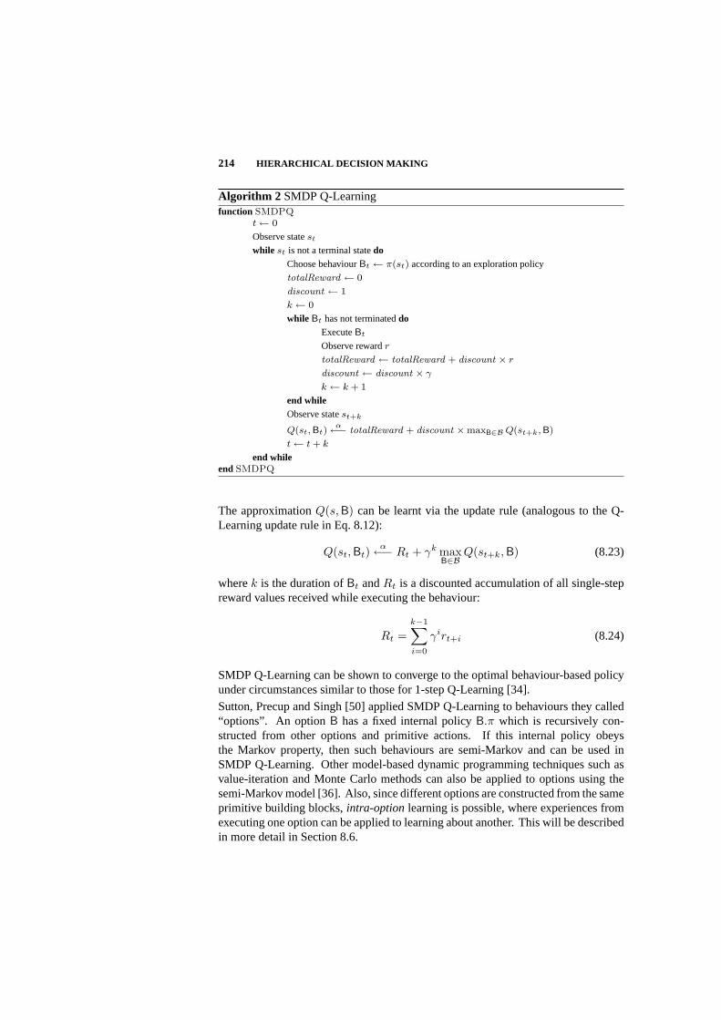
214 HIERARCHICAL DECISION MAKING
Algorithm 2 SMDP Q-Learningfunction SMDPQ
t ← 0
Observe statest
while st is not a terminal statedoChoose behaviourBt ← π(st) according to an exploration policy
totalReward ← 0
discount ← 1
k ← 0
while Bt has not terminateddoExecuteBt
Observe rewardr
totalReward ← totalReward + discount × r
discount ← discount × γ
k ← k + 1
end whileObserve statest+k
Q(st, Bt)α←− totalReward + discount ×maxB∈B Q(st+k, B)
t ← t + k
end whileendSMDPQ
The approximationQ(s, B) can be learnt via the update rule (analogous to the Q-Learning update rule in Eq. 8.12):
Q(st, Bt)α←− Rt + γk max
B∈BQ(st+k, B) (8.23)
wherek is the duration ofBt andRt is a discounted accumulation of all single-stepreward values received while executing the behaviour:
Rt =k−1∑
i=0
γirt+i (8.24)
SMDP Q-Learning can be shown to converge to the optimal behaviour-based policyunder circumstances similar to those for 1-step Q-Learning [34].
Sutton, Precup and Singh [50] applied SMDP Q-Learning to behaviours they called“options”. An optionB has a fixed internal policyB.π which is recursively con-structed from other options and primitive actions. If this internal policy obeysthe Markov property, then such behaviours are semi-Markov and can be used inSMDP Q-Learning. Other model-based dynamic programming techniques such asvalue-iteration and Monte Carlo methods can also be applied to options using thesemi-Markov model [36]. Also, since different options are constructed from the sameprimitive building blocks,intra-option learning is possible, where experiences fromexecuting one option can be applied to learning about another. This will be describedin more detail in Section 8.6.
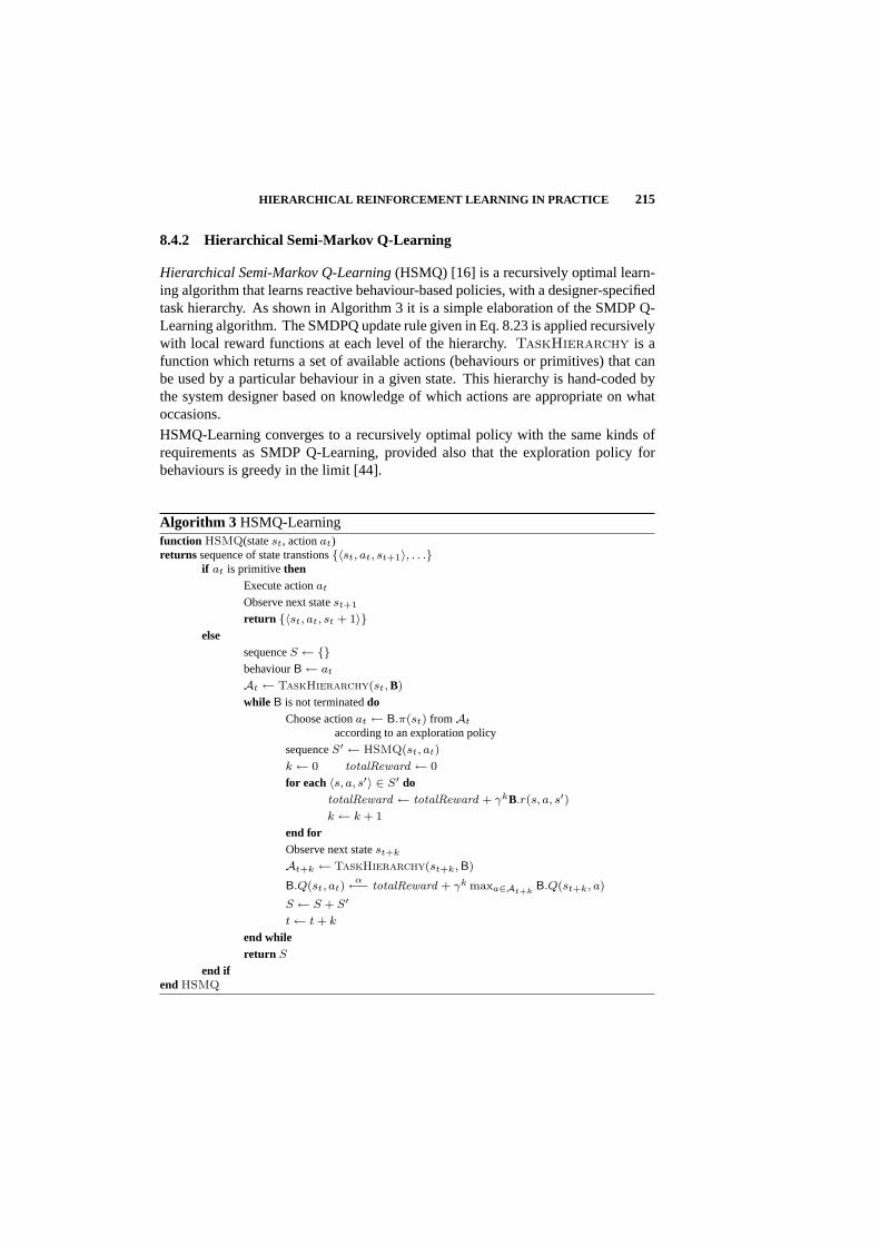
HIERARCHICAL REINFORCEMENT LEARNING IN PRACTICE 215
8.4.2 Hierarchical Semi-Markov Q-Learning
Hierarchical Semi-Markov Q-Learning(HSMQ) [16] is a recursively optimal learn-ing algorithm that learns reactive behaviour-based policies, with a designer-specifiedtask hierarchy. As shown in Algorithm 3 it is a simple elaboration of the SMDP Q-Learning algorithm. The SMDPQ update rule given in Eq. 8.23 is applied recursivelywith local reward functions at each level of the hierarchy.TaskHierarchy is afunction which returns a set of available actions (behaviours or primitives) that canbe used by a particular behaviour in a given state. This hierarchy is hand-coded bythe system designer based on knowledge of which actions are appropriate on whatoccasions.
HSMQ-Learning converges to a recursively optimal policy with the same kinds ofrequirements as SMDP Q-Learning, provided also that the exploration policy forbehaviours is greedy in the limit [44].
Algorithm 3 HSMQ-Learningfunction HSMQ(statest, actionat)returns sequence of state transtions〈st, at, st+1〉, . . .
if at is primitive thenExecute actionat
Observe next statest+1
return 〈st, at, st + 1〉else
sequenceS ← behaviourB ← at
At ← TaskHierarchy(st, B)
while B is not terminateddoChoose actionat ← B.π(st) fromAt
according to an exploration policy
sequenceS′ ← HSMQ(st, at)
k ← 0 totalReward ← 0
for each 〈s, a, s′〉 ∈ S′ dototalReward ← totalReward + γkB.r(s, a, s′)k ← k + 1
end forObserve next statest+k
At+k ← TaskHierarchy(st+k, B)
B.Q(st, at)α←− totalReward + γk maxa∈At+k
B.Q(st+k, a)
S ← S + S′
t ← t + k
end whilereturn S
end ifendHSMQ
216 HIERARCHICAL DECISION MAKING
8.4.3 MAXQ-Q
A more sophisticated algorithm for learning recursively optimal policies is Diet-terich’s MAXQ-Q [15]. The policies it learns are equivalent to those of HSMQ, but ituses a special decomposition of the state-action value function in order to learn themmore efficiently. MAXQ-Q relies on the observation that the value of a behaviourB as part of its parent behaviourP can be split into two parts: the reward expectedwhile executingB, and the discounted reward of continuing to executeP afterB hasterminated. That is:
P.Q(s, B) = P.I(s, B) + P.C(P, s, B) (8.25)
whereP.I(s,B) is the expected total discounted reward (according to the rewardfunction of the parent behaviourP) that is received while executing behaviourB frominitial states, andP.C(Bparent, s, Bchild) is the expected total reward of continuing toexecute behaviourBparentafterBchild has terminated, discounted appropriately to takeinto account the time spent inBchild. (Again with rewards calculated according to thebehaviourP.)
Furthermore theI(s, B) function can be recursively decomposed intoI andC viathe rule:
P.I(s, B) = maxa∈B.A
P.Q(s, a) (8.26)
There are several advantages to this decomposition, primarily of value in learningrecursively optimal Q-values. TheI andC functions can each be represented withcertain state abstractions that do not apply to both parts. The explanation is complexand beyond the scope of this review. For full details and pseudocode see [15].
8.4.4 Q-Learning with Hierarchies of Abstract Machines
Q-Learning with Hierarchies of Abstract Machines(HAMQ) [35] is an hierarchicallyoptimal learning algorithm that uses a more elaborate model to structure the policyspace. Behaviours are implemented ashierarchies of abstract machines(HAMs)which resemble finite-state machines, in that they include an internalmachine state.The state of the machine dictates the action it may take. Actions include: 1) perform-ing primitive actions, 2) calling other machines as subroutines, 3) making choices,4) terminating and returning control to the calling behaviour. Transitions betweenmachine states may be deterministic, stochastic or may rely on the state of the envi-ronment. Learning takes place at choice states only, where the behaviour must decidewhich of several internal state transitions to make. HAMs represent a compromisebetween hard-coded policies and fully-learnt policies. Some transitions can be hard-coded into the machine while others can be learnt. Thus they provide a means forbackground knowledge in the form of partial solutions to be specified.
Behaviours in HAMQ are merely a typographic convenience. In effect they arecompiled into a single abstract machine, consisting of action nodes and choice nodesonly. Algorithm 4 shows the Pseudocode for learning in such a machine.
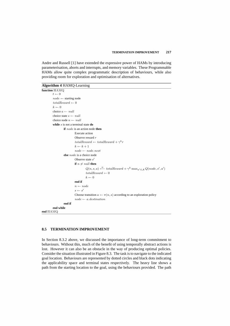
TERMINATION IMPROVEMENT 217
Andre and Russell [1] have extended the expressive power of HAMs by introducingparameterisation, aborts and interrupts, and memory variables. These ProgrammableHAMs allow quite complex programmatic description of behaviours, while alsoproviding room for exploration and optimisation of alternatives.
Algorithm 4 HAMQ-Learningfunction HAMQ
t ← 0
node ← starting node
totalReward ← 0
k ← 0
choicea ← null
choice states ← null
choice noden ← null
while s is not a terminal statedoif node is an action nodethen
Execute action
Observe rewardr
totalReward ← totalReward + γkr
k ← k + 1
node ← node.next
elsenode is a choice node
Observe states′
if n 6= null then
Q(n, s, a)α←− totalReward + γk maxa′∈AQ(node, s′, a′)
totalReward ← 0
k ← 0
end ifn ← node
s ← s′
Choose transitiona ← π(n, s) according to an exploration policy
node ← a.destination
end ifend while
endHAMQ
8.5 TERMINATION IMPROVEMENT
In Section 8.3.2 above, we discussed the importance of long-term commitment tobehaviours. Without this, much of the benefit of using temporally abstract actions islost. However it can also be an obstacle in the way of producing optimal policies.Consider the situation illustrated in Figure 8.3. The task is to navigate to the indicatedgoal location. Behaviours are represented by dotted circles and black dots indicatingthe applicability space and terminal states respectively. The heavy line shows apath from the starting location to the goal, using the behaviours provided. The path

218 HIERARCHICAL DECISION MAKING
travels from one termination state to the next, indicating that each behaviour is beingexecuted all the way to completion.
Start Goal
Fig. 8.3 A simple navigation task illustrating the advantage of termination improvement.The circles show the overlapping applicability spaces for a collection of hard-code navigationbehaviours. Each behaviour moves the agent towards the central landmark location (the blackdots). The heavy line indicates the standard policy with commitment to behaviours. Thelighter line indicates the path taken by a termination improved policy.
Compare this with the path shown by the lighter line. In this case each behaviouris executed only until a more appropriate behaviour becomes applicable. “Cuttingcorners” in this way results in a significantly shorter path, and a policy much closerto the optimal one.
This example is taken from the work of [45] who call this processterminationimprovement. They show how to produce such corner-cutting policies using hard-coded behaviours. Having already learnt an optimal policyπ using these behaviours,they transform it into an improvedinterrupted policyπ′ by prematurely interruptingan executing behaviourB wheneverQ(s,B) < V (s), i.e. when there is a betteralternative behaviour available. The resulting policy is guaranteed to be of equal orgreater efficiency than the original.
A similar approach can be applied to policies learnt using MAXQ-Q [15]. WhileMAXQ-Q is a recursively optimal learning algorithm, it nevertheless learns a valuefor each primitive action using the global reward function. In normal execution,actions are chosen on the basis of the local Q-value assigned to each by its callingbehaviour. However once such a recursively optimal policy has been learnt, it can beimproved by switching to selecting primitive actions based on their global Q-valueinstead. There is no longer any commitment to behaviours. Execution reverts tothe reactive semantics of monolithic Q-learning, and the hierarchy serves only s a

INTRA-BEHAVIOUR LEARNING 219
means to assign Q-values to primitives. This is called thehierarchical greedy policy,and is also guaranteed to be of equal or greater efficiency than the recursive policy.Furthermore, by continuing to update these Q-values, viapolling execution[23, 14],this policy can be further improved.
In both these algorithms it is important that the transformation is made to the policyonce an uninterrupted policy has already been learnt. If behaviours can be arbitrarilyinterrupted from the outset then the advantages of using temporally abstract actionsare lost. However in my own TRQ algorithm [39], I show that selective terminationimprovement can be done while learning is still ongoing, if we limit it to thoseoccasions in which we can prove that the executing behaviour is no longer appropriate.In TRQ this is done by giving behaviours abstract symbolic descriptions and usingthese descriptions to build high-level plans. A behaviour is only appropriate as longas it is recommended by the plan. If a behaviour is no longer appropriate then itmay be interrupted before normal termination without adversing affecting learningperformance.
8.6 INTRA-BEHAVIOUR LEARNING
When behaviours are constructed from a common set of primitive actions, in acommon Markov model, experiences gathered while executing one behaviour maystrongly overlap with those from another. If two behavioursB1 and B2 haveoverlapping applicability spaces and action sets, then whenB1 executes actiona ∈ B1.A ∩ B2.A in states ∈ B1.pre ∩ B2.pre then the resulting experience〈s, a, s′〉 can often be used to learn about bothB1 andB2.
There are two ways in which this information can be transferred fromB1 to B2:
1. It can be used to update both theinternalpolicy ofB2, through a method calledall-goals updating[23], and
2. It can be used to update theexternalpolicy which is callingB1 andB2, throughintra-option learning[36, 50].
8.6.1 All-goals updating
Q-Learning is what is termed anoff-policy learning algorithm [49]. This meansthat the update rule for the state-action value functionQ(s, a) (Eq. 8.12 above)does not rely on the actiona to be drawn from the current policy. In particular, ifwe are working in a recursively-optimal framework, in which there are behaviour-specific reward functions specifying local goals, then any experience〈s, a, s′〉 withs, s′ ∈ B.pre anda ∈ B.A can be used to update the state-action value functionB.Q(s, a) regardless of whether the experience was obtained while executingB itselfor another behaviour.

220 HIERARCHICAL DECISION MAKING
As a result, when multiple behaviours have overlapping applicability spaces andaction sets, then experiences from executing one behaviour can be used to improvethe policy of others. This is what Kaelbling callsall-goals updating[23].
This is also the case for the hierarchical extensions of Q-learning which we havepresented above, but is not true for all reinforcement learning algorithms.On-policyalgorithms, such as SARSA [38, 48] are not amenable to this kind of experiencesharing as they rely on the experiences used to update a policy being drawn from theexecution of that policy.
8.6.2 Intra-option learning
Whereas all-goals updating concerns updating the internal policies of overlappingbehaviours,intra-option learning[36, 50] updates the policy of the parent behaviourwhich calls the subtasksB1 andB2. In this caseB1 andB2 are assumed to be fixed-policy behaviours (options), although the technique can probably also be extendedto hierarchically-optimal or recursively-optimal learnt behaviours (no convergenceproof is yet available).
Intra-option learning is based on the observation that if a behaviourB dictates prim-itive actionat in statest, and then continues executing then:
Q?(st,B) = E(rt) + γ∑st+1
Tst+1st, atQ∗(st+1,B) (8.27)
i.e. the value of executingB in st is the immediate reward for executingat plus thediscounted value of continuing to executeB thereafter. Alternatively, ifB terminatesin statest+1 then:
Q?(st, B) = E(rt) + γ∑st+1
Tst+1st, at maxB′∈B
Q∗(st+1,B′) (8.28)
i.e. the value of executingB is the the immediate reward for executingat and thenthe discounted value of the subsequently chosen behaviour.
Based on this fact, we can construct aone-step intra-option Q-learningupdate rulewhich updates the state-behaviour valueQ(s, B) with B.π(s) = a based on theexperience〈s, a, r, s′〉, as follows:
Q(s,B) α←− r + γU(st+1, B) (8.29)
where:U(s, B) = (1− β(B, s))Q(s,B) + β(B, s)max
B′∈BQ(s,B′)
whereβ(B, s) denotes the probabilityB terminates in states.
Once again, this update rule does not rely on the experience necessarily resultingfrom the execution ofB as part of the parent policy. The experience may be drawnfrom the execution of behaviourB1 and used to update the value ofB2 provided that
CREATING BEHAVIOURS AND BUILDING HIERARCHIES 221
B1.π(s) = B2.π(s). So in this way we can improve our estimations of the value ofseveral “overlapping” behaviours based on the experience of executing only one.
Both this all-goals updating and intra-option learning increase the amount of com-putation done based on each experience gathered. This can potentially mean betterperformance with less experience, but it can also mean longer learning times due toexcess computation. There is a tradeoff between the experience and computation.Generally it is assumed that experience is the bottleneck in learning, and that compu-tation is relatively inexpensive, but as hierarchical methods grow more complex thisis an issue that is going to need to be addressed.
8.7 CREATING BEHAVIOURS AND BUILDING HIERARCHIES
As stated earlier, typically the hierarchy of behaviours is defined by a human designer.Many researchers have pointed to the desirability of automating this task (eg. [8, 17]).
One approach to this problem is the HEXQ algorithm [18]. This algorithm is anextension of MAXQ-Q which attempts to automatically decompose a problem intoa collection of subproblems. Sub-problems are created corresponding to particularvariables in the state-vector. Variables that change infrequently inspire behaviourswhich aim to cause those variables to change.
A similar approach is used by acQuire [32]. It uses exploration to identify “bot-tlenecks” in the state-space – states which are part of many trajectories through thespace. Bottleneck states are selected as subgoals for new behaviours.
Both these approaches implement a kind of uninformed behaviour invention, basedonly on the dynamics of the environment without any background knowledge.Rachel [39] adopts alternative approach. This system combines hierarchical rein-forcement learning with symbolic planning. Behaviours are specified by a trainingin abstract terms, in terms of their pre-conditions and goals. These specificationstake the form of teleo-operators [33], which are used in conjunction with symbolicplanning to build hierarchies of behaviours suited to a given task.
8.8 MODEL-BASED REINFORCEMENT LEARNING
As we said earlier, not all reinforcement learning algorithms are model-free likeQ-Learning and it’s derivatives. There are also many algorithms which attempt tolearn models of the transition and reward functionsTs′s, a and Rs′s, a, and thenuse these models to construct policies using dynamic programming methods such asvalue-iteration or policy-iteration (eg [47]). Such techniques have been somewhatless popular in practice as learning accurate models ofT andR has been found to bemore difficult than learning Q-values directly.

222 HIERARCHICAL DECISION MAKING
Nevertheless these technique have also been applied to the hierarchical reinforcementlearning problem, and model-based hierarchical algorithms exist (eg H-Dyna [42],SMDP Planning [36], abstract MDPs [17], and discrete-event models [30]).
It is unfortunate that model-based methods have apparently acquired second-classstatus in this field as there are potentially many ways in which a complete model, atmultiple levels of abstraction, could be exploited far beyond a particular task-specificset of Q-values. This is an area deserving further attention.
8.9 TOPICS FOR FUTURE RESEARCH
8.9.1 Recombination of different features
As we have described above, most hierarchical reinforcement learning algorithms areactually the combination of several independent features. These particular combina-tions are not necessarily forced, but are mainly accidental. Some of these featuresare:
1. Hierarchical vs Recursive optimality,
2. The MAXQ decomposition of the state-action value function,
3. The HAMQ programmable behaviour structure,
4. Termination improvement
5. Intra-option learning
It would certainly be worthwhile to investigate other recombinations of these features.There is no obvious reason, for example, why the MAXQ decomposition could notbe applied to to a hierarchically optimal learning algorithm; or the HAMQ frame-work used to structure recursively optimal behaviours with termination improvement.Some combinations may not work, but we cannot be sure of this until we explorethem.
8.9.2 Real-world Applications
As must be apparent from this chapter, the development of hierarchical reinforcementtheory and algorithms has been proceeding strongly in recent years. However thisdevelopment has far outstripped the use of these methods in non-trivial real-worldsituations. One piece of work stands out: Crites successful use of SMDP Q-learningto learn elevator control [11, 12]. Few others exist.
Hierarchical reinforcement learning is founded on the claim that hierarchy can helpus overcome the curse of dimensionality. The field has matured, the algorithms areavailable. Now it is time to prove that these claims are not empty.

CONCLUSION 223
8.10 CONCLUSION
Hierarchy has proven to be a rich source of development in reinforcement learning,producing both theoretical and practical advances. It has found a solid theoreticalmodel in Semi-Markov Decision Processes and has been growing strongly. Diversealgorithms have been built on this shared foundation, differing in terms of optimalitycriteria, action selection mechanisms, state-approximation, and, as always, terminol-ogy. In this chapter we have tried to unify these different approaches and show howtheir might be separated and recombined. It is our hope that this will give a coherentfoundation for future development and the application of these new ideas to solvinggreater problems.
Acknowledgments
I would like to thank Andrew Barto for reviewing several drafts of this report and providingmany valuable recommendations.

Bibliography
1. David Andre and Stuart J. Russell, “Programmable reinforcement learningagents,”Advances in Neural Information Processing Systems 12: Proceedingsof the 1999 Conference,pp. 1019-1025, 2000.
2. Leemon C. Baird, “Residual algorithms: Reinforcement learning with functionapproximation,” pp. 30-37, 1995.
3. Andrew G. Barto and Sridhar Mahadevan, “Recent advances in hierarchicalreinforcement learning,”Discrete-Event Dynamical Systems: Theory and Appli-cations,vol. 13, pp. 341-379, 2003.
4. J. Baxter, A. Tridgell, and L. Weaver, “Knightcap: A chess program that learnsby combining td(λ) with game-tree search,”Proceedings of the Fifteenth Inter-national Conference on Machine Learning,pp. 28-36, San Franciso, CA, 1998.
5. Richard Bellman,Dynamic Programming,Princeton University Press, 1957.
6. D. P. Bertsekas,Dynamic Programming: Deterministic and Stochastic Models,Prentice-Hall, Englewood Cliffs, NJ, 1987.
7. D. P. Bertsekas and J. N. Tsitsiklis,Neuro-Dynamic Programming,Athena Sci-entific, Belmont, MA, 1996.
8. Craig Boutilier, Thomas Dean, and Steve Hanks, “Decision-theoretic planning:Structural assumptions and computational leverage,”Journal of Artificial Intel-ligence Research,11:1–94, 1999.
9. Steven J. Bradtke and Michael O. Duff, “Reinforcement learning methods forcontinuous-time Markov decision problems,” In G. Tesauro, D. Touretzky, andT. Leen, editors,Advances in Neural Information Processing Systems,vol. 7,pp. 393–400. The MIT Press, 1995.
10. Rodney A. Brooks, “A robust layered control system for a mobile robot,”IEEEJournal of Robotics and Automation, RA-2(1):14–23, 1986.
11. Robert Harry Crites,Large-Scale Dynamic Optimization Using Teams of Rein-forcement Learning Agents,University of Massachusetts Amherst, 1996.
224

BIBLIOGRAPHY 225
12. Robert Harry Crites and Andrew G. Barto, “Elevator Group control using multi-ple reinforcement learning agents,”Machine Learning,vol. 33:2-3, pp. 235-262,1998.
13. Peter Dayan and Geoffrey E. Hinton, “Feudal reinforcement learning,”Advancesin Neural Information Processing Systems,vol. 5, pp. 271-278, 1992.
14. Thomas G. Dietterich, “The MAXQ method for hierarchical reinforcement learn-ing,” pp. 118-126, 1998.
15. Thomas G. Dietterich, “Hierarchical reinforcement learning with the MAXQvalue dunction decomposition,”Artitificial Intelligence, vol. 13, pp. 227-303,2000.
16. Thomas G. Dietterich, “An overview of MAXQ hierarchical reinforcement learn-ing,” In B. Y. Choueiry and T. Walsh, editors,Proceedings of the Symposiumon Abstraction, Reformulation and Approximation SARA 2000, Lecture Notes inArtificial Intelligence,pp. 26-44, New York, NY, 2000.
17. Milos Hauskrecht, Nicolas Meuleau, Leslie Pack Kaelbling, Thomas Dean,and Craig Boutilier, “Hierarchical solution of Markov decision processes us-ing macro-actions,”Uncertainty in Artificial Intelligence,pp. 220-229, 1998.
18. Bernhard Hengst, “Discovering hierarchy in reinforcement learning withHEXQ,” Proceedings of the Seventh International Conference on MachineLearning,1990.
19. Ronald A. Howard,Dynamic Programming and Markov Processes,The MITPress, Cambridge, MA, 1960.
20. Ronald A. Howard,Dynamic Probabilistic Systems: Semi-markov and DecisionProcesses,John Wiley and sons, New York, NY, 1971.
21. Glenn A. Iba, “A heuristic approach to the discovery of macro-operators,”Ma-chine Learning, vol. 3, pp. 285-317, 1989.
22. Tommi Jaakkola, Michael I. Jordan, and Satinder P. Singh, “On the convergenceof stochastic iterative dynamic programming algorithms,”Advances in NeuralInformation Processing Systems,vol. 6, The MIT Press, November, 1994.
23. Leslie Pack Kaelbling, “Hierarchical learning in stochastic domains: Prelim-inary results,”Proceedings of the Tenth International Conference on MachineLearning,1993.
24. Leslie Pack Kaelbling, Michael L. Littman, and Andrew P. Moore, “Reinforce-ment learning: A survey,”Journal of Artificial Intelligence Research, vol. 4,pp. 237-285, 1996.

226 BIBLIOGRAPHY
25. Craig A. Knoblock, “Search reduction in hierarchical problem solving,”Pro-ceedings of the Ninth National Conference on Artificial Intelligence (AAAI-91),vol. 2, pp.686-691, Anaheim, California, USA, 1991.
26. Richard E. Korf, “Planning as search: A quantitative approach,”Artificial Intel-ligence,vol. 33(1), pp. 65-88, 1987.
27. Long-Ji Lin.Reinforcement Learning for Robots Using Neural Networks,PhDthesis, School of Computer Science, Carnegie Mellon University, 1993.
28. P. Maes, “How to do the right thing,”Connection Science Journal, Special Issueon Hybrid Systems,vol. 1, 1990.
29. Sridhar Mahadevan, “Average reward reinforcement learning: Foundations, al-gorithms, and empirical results,”Machine Learning,vol. 22(1-3), pp. 159-195,1996.
30. Sridhar Mahadevan and Nikfar Khaleeli and Nicholas Marchalleck, “DesigningAgent Controllers using Discrete-Event Markov Models,”Working Notes of theAAAI Fall Symposium on Model-Directed Autonomous Systems,Cambridge,Massachusetts, 1997.
31. Maja J. Mataric, “Behaviour based control: Examples from navigation, learn-ing and group behaviour,”Journal of Experimental and Theoretical ArtificialIntelligence,vol. 9(2-3), 1996.
32. Amy McGovern and Andrew G. Barto, “Automatic discovery of subgoals inreinforcement learning using diverse density,” pp.361-368, 2001.
33. Nils J. Nilsson, “Teleo-reactive programs for agent control,”Journal of ArtificialIntelligence Research, vol. 1, pp. 139-158, 1994.
34. Ronald Parr,Hierarchical Control and learning for Markov decision processes,PhD thesis, University of California at Berkeley, 1998.
35. Ronald Parr and Stuart Russell, “Reinforcement learning with hierarchies ofmachines,” In Michael I. Jordan, Michael J. Kearns, and Sara A. Solla, editors,Advances in Neural Information Processing Systems,vol. 10,. The MIT Press,1998.
36. Doina Precup,Temporal Abstraction in Reinforcement Learning,University ofMassachusetts, Amherst, 2000.
37. Martin L. Puterman,Markov Decision Processes: Discrete Stochastic DynamicProgramming,John Wiley & Sons, Inc., New York, NY, 1994.
38. G. A. Rummery and M. Niranjan, “Online Q-learning using connectionist sys-tems,”Technical Report CUED/F-INFENG/TR 166,Cambridge University En-gineering Department, 1994.

BIBLIOGRAPHY 227
39. Malcolm R. K. Ryan,Hierarchical Reinforcement Learning: A Hybrid Ap-proach,PhD thesis, University of New South Wales, 2002.
40. Earl D. Sacerdoti, Planning in a hierarchy of abstraction spaces,Artificial Intel-ligence,vol. 5(2), pp. 115-135, 1974.
41. A. Schwartz, “A reinforcement learning method for maximizing undiscountedrewards,”Proceedings of the Tenth International Conference on Machine Learn-ing, 1993.
42. Satinder P. Singh, “Reinforcement Learning with a Hierarchy of Abstract Mod-els,” Proceedings of the Tenth National Conference on Artifical Intelligence,1992.
43. Satinder P. Singh, “Reinforcement learning algorithms for average-payoff marko-vian decision processes,”National Conference on Artificial Intelligence,pp. 700-705, 1994.
44. Satinder P. Singh, Tommi Jaakkola, Michael L. Littman, and Csaba Szepes-vari, “Convergence results for single-step on-policy reinforcement-learning al-gorithms,”Machine Learning, vol. 38(3), pp. 287-308, 2000.
45. R. S. Sutton, S. Singh, D. Precup, and B. Ravindran, “Improved switchingamong temporally abstract actions,”Advances in Neural Information ProcessingSystems,vol. 11, The MIT Press, 1999.
46. Richard S. Sutton, “Implementation details for the TD(λ) procedure for the caseof vector predictions and backpropagation,”Technical Report TN87-509.1,GTELaboratories, 1987.
47. Richard S. Sutton, “Integrated Architectures for Learning, Planning and ReactingBased on Approximating Dynamic Programming,”Proceedings of the SeventhInternational Conference on Machine Learning,San Franciso, CA, 1990.
48. Richard S. Sutton, “Generalisation in reinforcement learning successful exam-ples using sparse coarse coding,”Advances in Neural Neural Information Pro-cessing Systems,1995.
49. Richard S. Sutton and Andrew G. Barto,Reinforcement Learning: An Introduc-tion, The MIT Press, Cambridge, MA, 1998.
50. Richard S. Sutton, Doina Precup, and Satinder P. Singh, “Between MDPs andsemi-MDPs: A framework for temporal abstraction in reinforcement learning,”Artificial Intelligence,vol. 112(1-2), pp. 181-211, 1999.
51. G. Tesauro, “Td-gammon, a self-teaching backgammon program achievesmaster-level play,”Neural Computation, vol. 6, pp. 215-219, 1994.
228 BIBLIOGRAPHY
52. S. B. Thrun, “The role of exploration in learning control with neural networks,” InD. A. White and D. A. Sofge, editors,Handbook of Intelligent Control: Neural,Fuzzy and Adaptive Approaches,Florence, Kentucky, 1992.
53. John N. Tsitsiklis, “Asynchronous stochastic approximation and Q-learning,”Machine Learning, vol. 16(3), September, 1994.
54. Christopher. J. C. H. Watkins,Learning from Delayed Rewards,PhD thesis,King’s College, Cambridge, England, 1989.
55. Christopher. J. C. H. Watkins and Peter Dayan, “Q-learning,”Machine Learning,vol. 8(3), pp. 279-292, 1992.
56. W. Zhang and T. G. Dietterich, “A reinforcement learning approach to job-shopscheduling,”Proceedings of the Fourteenth International Joint Conference onArtificial Intelligence,1995.

Part II
Technical Advances

9 Improved Temporal DifferenceMethods with Linear FunctionApproximation
DIMITRI P. BERTSEKAS and ANGELIA NEDICHMassachusetts Institute of Technology Alphatech, Inc.VIVEK S. BORKARTata Institute of Fundamental Research
Editor’s Summary: This chapter considers temporal difference algorithms withinthe context of infinite-horizon finite-state dynamic programming problems with dis-counted cost and linear cost function approximation. This problem arises as asubproblem in the policy iteration method of dynamic programming. Additionaldiscussions of such problems can be found in Chapters 12 and 6. The advantage ofthe method presented here is that this is the first iterative temporal difference methodthat converges without requiring a diminishing step size. The chapter discusses theconnections with Suttonfls TD(λ) and with various versions of least-squares thatare based on value-iteration. It is shown using both analysis and experiments thatthe proposed method is substantially faster, simpler, and more reliable than TD(λ).Comparisons are also made with the LSTD method of Boyan and Bradtke and Barto.
9.1 INTRODUCTION
In this paper, we analyze methods for approximate evaluation of the cost-to-go func-tion of a stationary Markov chain within the framework of infinite-horizon discounteddynamic programming. We denote the states by1, . . . , n, the transition probabili-ties bypij , i, j = 1, . . . , n, and the corresponding costs byαtg(i, j), whereα is adiscount factor with0 < α < 1. We want to evaluate the long-term expected costcorresponding to each initial statei, given by
J(i) = E
[ ∞∑t=0
αtg(it, it+1)∣∣∣ i0 = i
], ∀ i = 1, . . . , n,
231

232 IMPROVED TD METHODS WITH LINEAR FUNCTION APPROXIMATION
whereit denotes the state at timet. This problem arises as a subproblem in the policyiteration method of dynamic programming, and its variations, such as modifiedpolicy iteration, optimistic policy iteration, andλ-policy iteration (see Bertsekas andTsitsiklis [4], Bertsekas [3], and Puterman [15] for extensive discussions of thesemethods).
The cost functionJ(i) is approximated by a linear function of the form
J(i, r) = φ(i)′r, ∀ i = 1, . . . , n,
whereφ(i) is ans-dimensional feature vector, associated with the statei, with com-ponentsφ1(i), . . . , φs(i), whiler is a weight vector with componentsr(1), . . . , r(s).(Throughout the paper, vectors are viewed as column vectors, and a prime denotestransposition.)
Our standing assumptions are:
(a) The Markov chain has steady-state probabilitiesπ(1), . . . , π(n) which arepositive, i.e.,
limt→∞
P [it = j | i0 = i] = π(j) > 0, ∀ i, j.
(b) The matrixΦ given by
Φ =
− φ(1)′ −
...− φ(n)′ −
has ranks.
The TD(λ) method with function approximation was originally proposed by Sutton[17], and its convergence has been analyzed by several authors, including Dayan [8],Gurvits, Lin, and Hanson [10], Pineda [14], Tsitsiklis and Van Roy [19], and VanRoy [18]. We follow the line of analysis and Tsitsiklis and Van Roy, who have alsoconsidered a discounted problem under the preceding assumptions on the existenceof steady-state probabilities and rank ofΦ.
The algorithm, described in several references, including the books by Bertsekas andTsitsiklis [4], and Sutton and Barto [16], generates an infinitely long trajectory ofthe Markov chain(i0, i1, . . .) using a simulator, and at timet iteratively updates thecurrent estimatert using an iteration that depends on a fixed scalarλ ∈ [0, 1], and onthe temporal differences
dt(ik, ik+1) = g(ik, ik+1) + αφ(ik+1)′rt − φ(ik)′rt, ∀ t = 0, 1, . . . , ∀ k ≤ t.
Tsitsiklis and Van Roy [19] have introduced the linear system of equations
Ar + b = 0,

INTRODUCTION 233
whereA andb are given by
A = Φ′D(αP − I)∞∑
m=0
(αλP )mΦ, b = Φ′D∞∑
m=0
(αλP )mg, (9.1)
P is the transition probability matrix of the Markov chain,D is the diagonal matrixwith diagonal entriesπ(i), i = 1, . . . , n,
D =
π(1) 0 · · · 00 π(2) · · · 0
· · ·0 0 · · · π(n)
, (9.2)
andg is the vector with componentsg(i) =∑n
j=1 pijg(i, j). They have shown thatTD(λ) converges to the unique solutionr∗ = −A−1b of the systemAr + b = 0, andthat the error between the corresponding approximationΦr∗ and the true cost-to-govectorJ satisfies
‖Φr∗ − J‖D ≤ 1− αλ
1− α‖ΠJ − J‖D,
where‖ · ‖D is the weighted norm corresponding to the matrixD (i.e., ‖x‖D =√x′Dx), andΠ is the matrix given byΠ = Φ(Φ′DΦ)−1Φ′D. (Note thatΠJ − J
is the difference betweenJ and its projection, with respect to the weighted norm, onthe range of the feature matrixΦ.)
The essence of the Tsitsiklis and Van Roy analysis is to write the TD(λ) algorithm as
rt+1 = rt + γt(Art + b) + γt(Ξtrt + ξt), t = 0, 1, . . . , (9.3)
whereγt is a positive stepsize, andΞt andξt are some sequences of random matricesand vectors, respectively, that depend only on the simulated trajectory (so they areindependent ofrt), and asymptotically have zero mean. A key to the convergenceproof is that the matrixA is negative definite, so it has eigenvalues with negative realparts, which implies in turn that the matrixI + γtA has eigenvalues within the unitcircle for sufficiently smallγt. However, in TD(λ) it is essential that the stepsizeγt
be diminishing to 0, both because a smallγt is needed to keep the eigenvalues ofI + γtA within the unit circle, and also becauseΞt andξt do not converge to 0.
In this paper, we focus on theλ-least squares policy evaluation method (λ-LSPEfor short), proposed and analyzed by Nedic and Bertsekas [13]. This algorithm wasmotivated as a simulation-based implementation of theλ-policy iteration method,proposed by Bertsekas and Ioffe [2] (also described in Bertsekas and Tsitsiklis [4],Section 2.3.1). In fact the method of this paper was also stated (without convergenceanalysis), and was used with considerable success by Bertsekas and Ioffe [2] [seealso Bertsekas and Tsitsiklis [4], Eq. (8.6)] to train a tetris playing program – achallenging large-scale problem that TD(λ) failed to solve. In this paper, rather thanfocusing on the connection withλ-policy iteration, we emphasize a connection with(multistep) value iteration (see Section 9.4).

234 IMPROVED TD METHODS WITH LINEAR FUNCTION APPROXIMATION
The λ-LSPE method, similar to TD(λ), generates an infinitely long trajectory(i0,i1, . . .) using a simulator. At each timet, it finds the solutionrt of a least squaresproblem,
rt = arg minr
t∑m=0
(φ(im)′r − φ(im)′rt −
t∑
k=m
(αλ)k−mdt(ik, ik+1)
)2
, (9.4)
and computes the new vectorrt+1 according to
rt+1 = rt + γ(rt − rt), (9.5)
whereγ is a positive stepsize. The initial weight vectorr0 is chosen independentlyof the trajectory(i0, i1, . . .).It can be argued thatλ-LSPE is a “scaled” version of TD(λ). In particular, from theanalysis of Nedic and Bertsekas ([13], p. 101; see also Section 9.3), it follows thatthe method takes the form
rt+1 = rt + γ(Φ′DΦ)−1(Art + b) + γ(Ztrt + ζt), t = 0, 1, . . . , (9.6)
whereγ is a positive stepsize, andZt andζt are some sequences of random matricesand vectors, respectively, that converge to 0 with probability 1. It was shown in[13] that when the stepsize is diminishing rather than being constant, the methodconverges with probability 1 to the same limit as TD(λ), the unique solutionr∗ ofthe systemAr + b = 0 (convergence for a constant stepsize was conjectured but notproved).
One of the principal results of this paper is that the scaling matrix(Φ′DΦ)−1 is“close" enough to−A−1 so that, based also on the negative definiteness ofA, thestepsizeγ = 1 leads to convergence for allλ ∈ [0, 1], i.e., the matrixI+(Φ′DΦ)−1Ahas eigenvalues that are within the unit circle of the complex plane. In fact, we cansee thatA may be written in the alternative form
A = Φ′D(M − I)Φ, M = (1− λ)∞∑
m=0
λm(αP )m+1,
so that forλ = 1, the eigenvalues ofI + (Φ′DΦ)−1A are all equal to 0. Wewill also show that asλ decreases towards 0, the region where the eigenvalues ofI + (Φ′DΦ)−1A lie expands, but stays within the interior of the unit circle.
By comparing the iterations (9.3) and (9.6), we see that TD(λ) andλ-LSPE have acommon structure – a deterministic linear iteration plus noise that tends to 0 withprobability 1. However, the convergence rate of the deterministic linear iteration isgeometric in the case ofλ-LSPE, while it is slower than geometric in the case ofTD(λ), because the stepsizeγt must be diminishing. This indicates thatλ-LSPEhas a significant rate of convergence advantage over TD(λ). At the same time, witha recursive Kalman filter-like implementation discussed in [13],λ-LSPE does not

INTRODUCTION 235
require much more overhead per iteration than TD(λ) [the associated matrix inversionat each iteration requires onlyO(s2) computation using the results of the inversionat the preceding iteration, wheres is the dimension ofr].
For some further insight on the relation ofλ-LSPE withγ = 1 and TD(λ), let usfocus on the case whereλ = 0. TD(0) has the form
rt+1 = rt + γtφ(it)dt(it, it+1), (9.7)
while 0-LSPE has the form
rt+1 = arg minr
t∑m=0
(φ(im)′r − φ(im)′rt − dt(im, im+1)
)2(9.8)
[cf. Eq. (9.4)]. We note that the gradient of the least squares sum above is
−2t∑
m=0
φ(im)dt(im, im+1).
Asymptotically, in steady-state, the expected values of all the terms in this sum areequal, and each is proportional to the expected value of the termφ(it)dt(it, it+1)in the TD(0) iteration (9.7). Thus, TD(0)updatesrt along the gradient of the leastsquares sum of 0-LSPE, plus stochastic noise that asymptotically has zero mean. Thisinterpretation also holds for other values ofλ 6= 0, as will be discussed in Section9.4.
Another class of temporal difference methods, parameterized byλ ∈ [0, 1], hasbeen introduced by Boyan [6], following the work by Bradtke and Barto [7] whoconsidered the caseλ = 0. These methods, known as Least Squares TD (LSTD), alsoemploy least squares and have guaranteed convergence to the same limit as TD(λ)andλ-LSPE, as shown by Bradtke and Barto [7] for the caseλ = 0, and by Nedic andBertsekas [13] for the caseλ ∈ (0, 1]. Konda [12] has derived the asymptotic meansquared error of a class of recursive and nonrecursive temporal difference methods[including TD(λ) and LSTD, but not including LSPE], and have found that LSTDhas optimal asymptotic convergence rate within this class. The LSTD method is notiterative, but instead it evaluates the simulation-based estimatesAt andbt of (t+1)Aand(t + 1)b, given by
At =t∑
m=0
zm
(αφ(im+1)′ − φ(im)′
),
bt =t∑
m=0
zmg(im, im+1), zm =m∑
k=0
(αλ)m−kφ(ik),
(see Section 9.3), and estimates the solutionr∗ of the systemAr + b = 0 by
rt+1 = −A−1t bt.
236 IMPROVED TD METHODS WITH LINEAR FUNCTION APPROXIMATION
We argue in Section 9.5 that LSTD andλ-LSPE have comparable asymptotic perfor-mance, although there are significant differences in the early iterations. In fact, theiterates of LSTD andλ-LSPE converge to each other faster than they converge tor∗.Some insight into the comparability of the two methods can be obtained by verifyingthat the LSTD estimatert+1 is also the unique vectorr satisfying
r = arg minr
t∑m=0
(φ(im)′r − φ(im)′r −
t∑
k=m
(αλ)k−md(ik, ik+1; r)
)2
, (9.9)
whered(ik, ik+1; r) = g(ik, ik+1) + αφ(ik+1)′r − φ(ik)′r.
While finding r that satisfies Eq. (9.9) is not a least squares problem, its similaritywith the least squares problem solved by LSPE [cf. Eq. (9.4)] is evident.
We note, however, that LSTD and LSPE may differ substantially in the early iterations.Furthermore, LSTD is a pure simulation method that cannot take advantage of a goodinitial choicer0. This is a significant factor in favor ofλ-LSPE in a major context,namely optimistic policy iteration [4], where the policy used is changed (using apolicy improvement mechanism) after a few simulated transitions. Then, the use ofthe latest estimate ofr to start the iterations corresponding to a new policy, as wellas a small stepsize (to damp oscillatory behavior following a change to a new policy)is essential for good overall performance.
The algorithms and analysis of the present paper, in conjunction with existing re-search, support a fairly comprehensive view of temporal difference methods withlinear function approximation. The highlights of this view are as follows:
(1) Temporal difference methods fundamentally emulate value iteration methodsthat aim to solve a Bellman equation that corresponds to a multiple-transitionversion of the given Markov chain, and depends onλ (see Section 9.4).
(2) The emulation of thekth value iteration is approximate through linear functionapproximation, and solution of the least squares approximation problem (9.4)that involves the simulation data(i0, i1, . . . , it) up to timet.
(3) The least squares problem (9.4) is fully solved at timet byλ-LSPE, but is solvedonly approximately, by a single gradient iteration (plus zero-mean noise), byTD(λ) (see Section 9.4).
(4) LSPE and LSTD have similar asymptotic performance, but may differ substan-tially in the early iterations. Furthermore, LSPE can take advantage of goodinitial estimates ofr∗, while LSTD, as presently known, can not.
The paper is organized as follows. In Section 9.2, we derive a basic lemma regardingthe location of the eigenvalues of the matrixI +(Φ′DΦ)−1A. In Section 9.3, we usethis lemma to show convergence ofλ-LSPE with probability 1 for any stepsizeγ in arange that includesγ = 1. In Section 9.4, we derive the connection ofλ-LSPE with
PRELIMINARY ANALYSIS 237
various forms of approximate value iteration. Based on this connection, we discusshow our line of analysis extends to other types of dynamic programming problems. InSection 9.5, we discuss the relation betweenλ-LSPE and LSTD. Finally, in Section9.6 we present computational results showing thatλ-LSPE is dramatically faster thanTD(λ), and also simpler because it does not require any parameter tuning for thestepsize selection method.
9.2 PRELIMINARY ANALYSIS
In this section we prove some lemmas relating to the transition probability matrixP , the feature matrixΦ, and the associated matricesD andA of Eqs. (9.2) and(9.1). We denote byR andC the set of real and complex numbers, respectively,and byRn andCn the spaces ofn-dimensional vectors with real and with complexcomponents, respectively. The complex conjugate of a complex numberz is denotedz. The complex conjugate of a vectorz ∈ Cn, is the vector whose components arethe complex conjugates of the components ofz, and is denotedz. The modulus
√zz
of a complex numberz is denoted by|z|. We consider two norms onCn, the standardnorm, defined by
‖z‖ = (z′z)1/2 =
(n∑
i=1
|zi|2)1/2
, ∀ z = (z1, . . . , zn) ∈ Cn,
and the weighted norm, defined by
‖z‖D = (z′Dz)1/2 =
(n∑
i=1
p(i)|zi|2)1/2
, ∀ z = (z1, . . . , zn) ∈ Cn.
The following lemma extends, from<n to Cn, a basic result of Tsitsiklis and VanRoy [19].
Lemma 9.2.1 For all z ∈ Cn, we have‖Pz‖D ≤ ‖z‖D.
Proof: For any z = (z1, . . . , zn) ∈ Cn, we have, using the defining property∑ni=1 p(i)pij = p(j) of the steady-state probabilities,
‖Pz‖2D = z′P ′DPz
=n∑
i=1
p(i)
n∑
j=1
pij zj
n∑
j=1
pijzj

238 IMPROVED TD METHODS WITH LINEAR FUNCTION APPROXIMATION
≤n∑
i=1
p(i)
n∑
j=1
pij |zj |
2
≤n∑
i=1
p(i)n∑
j=1
pij |zj |2
=n∑
j=1
n∑
i=1
p(i)pij |zj |2
=n∑
j=1
p(j)|zj |2
= ‖z‖2D,
where the first inequality follows sincexy + xy ≤ 2|x| |y| for any two complexnumbersx andy, and the second inequality follows by applying Jensen’s inequality.
¥The next lemma is the key to the convergence proof of the next section.
Lemma 9.2.2 The eigenvalues of the matrixI +(Φ′DΦ)−1A lie within the circle ofradiusα(1− λ)/(1− αλ).
Proof: We haveA = Φ′D(M − I)Φ,
where
M = (1− λ)∞∑
m=0
λm(αP )m+1,
so that(Φ′DΦ)−1A = (Φ′DΦ)−1Φ′DMΦ− I.
HenceI + (Φ′DΦ)−1A = (Φ′DΦ)−1Φ′DMΦ.
Let β be an eigenvalue ofI + (Φ′DΦ)−1A and letz be a corresponding eigenvector,so that
(Φ′DΦ)−1Φ′DMΦz = βz.
LettingW =
√DΦ,
we have(W ′W )−1W ′√DMΦz = βz,
from which, by left-multiplying withW , we obtain
W (W ′W )−1W ′√DMΦz = βWz. (9.10)

CONVERGENCE ANALYSIS 239
The norm of the right-hand side of Eq. (9.10) is
‖βWz‖ = |β| ‖Wz‖ = |β|√
zΦ′DΦz = |β| ‖Φz‖D. (9.11)
To estimate the norm of the left-hand side of Eq. (9.10), first note that
‖W (W ′W )−1W ′√DMΦz‖ ≤ ‖W (W ′W )−1W ′‖ ‖√
DMΦz‖‖W (W ′W )−1W ′‖ ‖
√DMΦz‖ = ‖W (W ′W )−1W ′‖ ‖MΦz‖D,
and then note also thatW (W ′W )−1W ′ is a projection matrix [i.e., forx ∈ <n,W (W ′W )−1W ′x is the projection ofx on the subspace spanned by the columns ofW ], so that‖W (W ′W )−1W ′x‖ ≤ ‖x‖, from which
‖W (W ′W )−1W ′‖ ≤ 1.
Thus we have
‖W (W ′W )−1W ′√DMΦz‖ ≤ ‖MΦz‖D
=
∥∥∥∥∥(1− λ)∞∑
m=0
λmαm+1Pm+1Φz
∥∥∥∥∥D
≤ (1− λ)∞∑
m=0
λmαm+1‖Pm+1Φz‖D
≤ (1− λ)∞∑
m=0
λmαm+1‖Φz‖D
=α(1− λ)1− αλ
‖Φz‖D, (9.12)
where the last inequality follows by repeated use of Lemma 9.2.1. By comparingEqs. (9.12) and (9.11), and by taking into account thatΦz 6= 0 (sinceΦ has fullrank), we see that
|β| ≤ α(1− λ)1− αλ
.
¥
9.3 CONVERGENCE ANALYSIS
We will now use Lemma 9.2.2 to prove the convergence ofλ-LSPE. It is shown inNedic and Bertsekas [13] that the method is given by
rt+1 = rt + γB−1t (Atrt + bt), ∀ t, (9.13)
240 IMPROVED TD METHODS WITH LINEAR FUNCTION APPROXIMATION
where
Bt =t∑
m=0
φ(im)φ(im)′, At =t∑
m=0
zm
(αφ(im+1)′ − φ(im)′
), (9.14)
bt =t∑
m=0
zmg(im, im+1), zm =m∑
k=0
(αλ)m−kφ(ik). (9.15)
[Note that if in the early iterations,∑t
m=0 φ(im)φ(im)′ is not invertible, we may addto it a small positive multiple of the identity, or alternatively we may replace inverseby pseudoinverse. Such modifications are inconsequential and will be ignored in thesubsequent analysis; see also [13].] We can rewrite Eq. (9.13 as
rt+1 = rt + γB−1
t (Atrt + bt), ∀ t,
where
Bt =Bt
t + 1, At =
At
t + 1, bt =
bt
t + 1.
Using the analysis of [13] (see the proof of Prop. 3.1, p. 108), it follows that withprobability 1, we have
Bt → B, At → A, bt → b,
whereB = Φ′DΦ,
andA andb are given by Eq. (9.1).
Thus, we may write iteration (9.13) as
rt+1 = rt + γ(Φ′DΦ)−1(Art + b) + γ(Ztrt + ζt), t = 0, 1, . . . , (9.16)
whereZt = B
−1
t At −B−1A, ζt = B−1
t bt −B−1b.
Furthermore, with probability 1, we have
Zt → 0, ζt → 0.
We are now ready to prove our convergence result.
Proposition 9.3.1 The sequence generated by theλ-LSPE method converges tor∗ =−A−1b with probability 1, provided that the constant stepsizeγ satisfies
0 < γ <2− 2αλ
1 + α− 2αλ.

RELATIONS BETWEEN λ-LSPE AND VALUE ITERATION 241
Proof: If we write the matrixI + γ(Φ′DΦ)−1A as
(1− γ)I + γ(I + (Φ′DΦ)−1A
),
we see, using Lemma 9.2.2, that its eigenvalues lie within the circle that is centeredat1− γ and has radius
γα(1− λ)1− αλ
.
It follows by a simple geometrical argument that this circle is strictly contained withinthe unit circle if and only ifγ lies in the range between 0 and(2−2αλ)/(1+α−2αλ).Thus for eachγ within this range, the spectral radius ofI + γ(Φ′DΦ)−1A is lessthan 1, and there exists a norm‖ · ‖w over<n and anε > 0 (depending onγ) suchthat
‖I + γ(Φ′DΦ)−1A‖w < 1− ε.
Using the equationb = −Ar∗, we can write the iteration (9.16) as
rt+1− r∗ =(I +γ(Φ′DΦ)−1A+γZt
)(rt− r∗)+γ(Ztr
∗+ ζt), t = 0, 1, . . . .
For any simulated trajectory such thatZt → 0 andζt → 0, there exists an indextsuch that
‖I + γ(Φ′DΦ)−1A + γZt‖w < 1− ε, ∀ t ≥ t.
Thus, for sufficiently larget, we have
‖rt+1 − r∗‖w ≤ (1− ε)‖rt − r∗‖w + γ‖Ztr∗ + ζt‖w.
SinceZtr∗ + ζt → 0, it follows that rt − r∗ → 0. Since the set of simulated
trajectories such thatZt → 0 andζt → 0 is a set of probability 1, it follows thatrt → r∗ with probability 1. ¥Note that asλ decreases, the range of stepsizesγ that lead to convergence is reduced.However, this range always contains the stepsizeγ = 1.
9.4 RELATIONS BETWEEN λ-LSPE AND VALUE ITERATION
In this section, we will discuss a number of value iteration ideas, which underlie thestructure ofλ-LSPE. These connections become most apparent when the stepsize isconstant and equal to 1 (γ ≡ 1), which we will assume in our discussion.
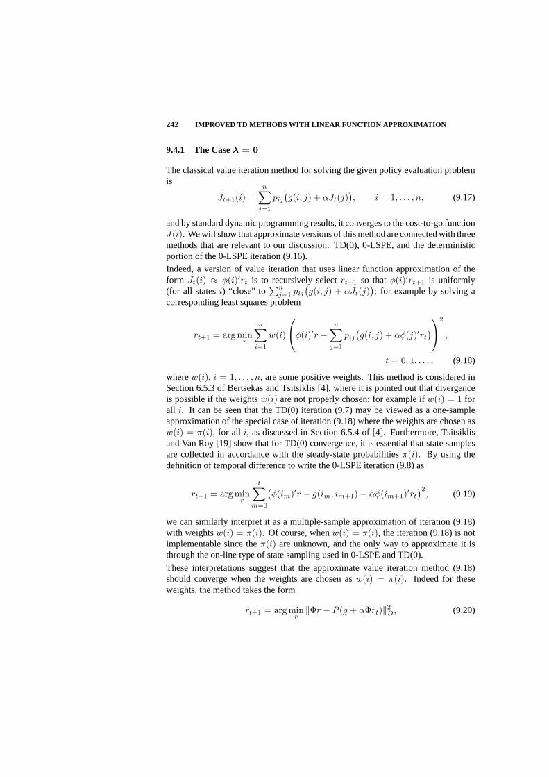
242 IMPROVED TD METHODS WITH LINEAR FUNCTION APPROXIMATION
9.4.1 The Caseλ = 0
The classical value iteration method for solving the given policy evaluation problemis
Jt+1(i) =n∑
j=1
pij
(g(i, j) + αJt(j)
), i = 1, . . . , n, (9.17)
and by standard dynamic programming results, it converges to the cost-to-go functionJ(i). We will show that approximate versions of this method are connected with threemethods that are relevant to our discussion: TD(0), 0-LSPE, and the deterministicportion of the 0-LSPE iteration (9.16).
Indeed, a version of value iteration that uses linear function approximation of theform Jt(i) ≈ φ(i)′rt is to recursively selectrt+1 so thatφ(i)′rt+1 is uniformly(for all statesi) “close" to
∑nj=1 pij
(g(i, j) + αJt(j)
); for example by solving a
corresponding least squares problem
rt+1 = arg minr
n∑
i=1
w(i)
φ(i)′r −
n∑
j=1
pij
(g(i, j) + αφ(j)′rt
)
2
,
t = 0, 1, . . . , (9.18)
wherew(i), i = 1, . . . , n, are some positive weights. This method is considered inSection 6.5.3 of Bertsekas and Tsitsiklis [4], where it is pointed out that divergenceis possible if the weightsw(i) are not properly chosen; for example ifw(i) = 1 forall i. It can be seen that the TD(0) iteration (9.7) may be viewed as a one-sampleapproximation of the special case of iteration (9.18) where the weights are chosen asw(i) = π(i), for all i, as discussed in Section 6.5.4 of [4]. Furthermore, Tsitsiklisand Van Roy [19] show that for TD(0) convergence, it is essential that state samplesare collected in accordance with the steady-state probabilitiesπ(i). By using thedefinition of temporal difference to write the 0-LSPE iteration (9.8) as
rt+1 = arg minr
t∑m=0
(φ(im)′r − g(im, im+1)− αφ(im+1)′rt
)2, (9.19)
we can similarly interpret it as a multiple-sample approximation of iteration (9.18)with weightsw(i) = π(i). Of course, whenw(i) = π(i), the iteration (9.18) is notimplementable since theπ(i) are unknown, and the only way to approximate it isthrough the on-line type of state sampling used in 0-LSPE and TD(0).
These interpretations suggest that the approximate value iteration method (9.18)should converge when the weights are chosen asw(i) = π(i). Indeed for theseweights, the method takes the form
rt+1 = arg minr‖Φr − P (g + αΦrt)‖2D, (9.20)
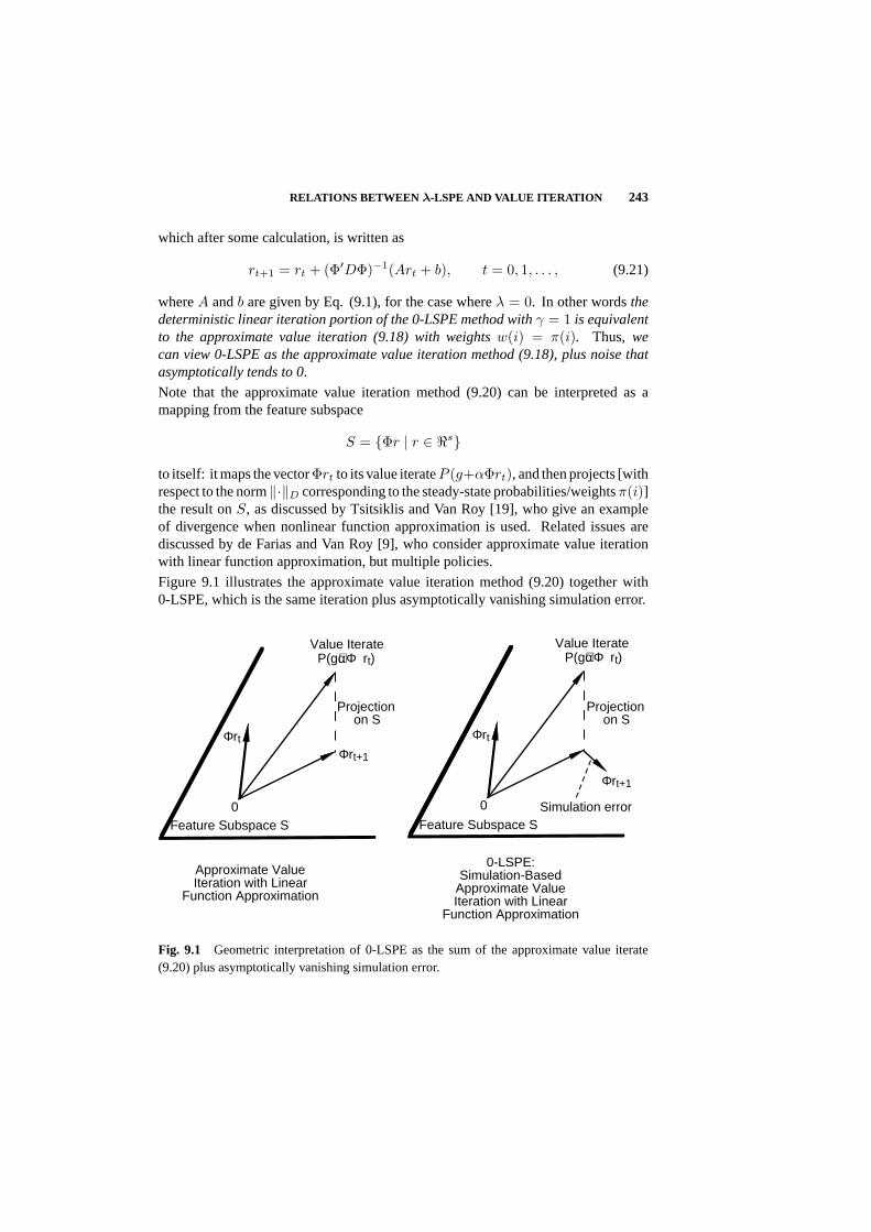
RELATIONS BETWEEN λ-LSPE AND VALUE ITERATION 243
which after some calculation, is written as
rt+1 = rt + (Φ′DΦ)−1(Art + b), t = 0, 1, . . . , (9.21)
whereA andb are given by Eq. (9.1), for the case whereλ = 0. In other wordsthedeterministic linear iteration portion of the 0-LSPE method withγ = 1 is equivalentto the approximate value iteration (9.18) with weightsw(i) = π(i). Thus, wecan view 0-LSPE as the approximate value iteration method (9.18), plus noise thatasymptotically tends to 0.
Note that the approximate value iteration method (9.20) can be interpreted as amapping from the feature subspace
S = Φr | r ∈ <s
to itself: it maps the vectorΦrt to its value iterateP (g+αΦrt), and then projects [withrespect to the norm‖·‖D corresponding to the steady-state probabilities/weightsπ(i)]the result onS, as discussed by Tsitsiklis and Van Roy [19], who give an exampleof divergence when nonlinear function approximation is used. Related issues arediscussed by de Farias and Van Roy [9], who consider approximate value iterationwith linear function approximation, but multiple policies.
Figure 9.1 illustrates the approximate value iteration method (9.20) together with0-LSPE, which is the same iteration plus asymptotically vanishing simulation error.
Feature Subspace S
Φrt
P(g+αΦrt)
0
Φrt+1
Feature Subspace S
Φrt
0
Φrt+1
Simulation error
Approximate ValueIteration with Linear
Function Approximation
0-LSPE:Simulation-Based
Approximate ValueIteration with Linear
Function Approximation
P(g+αΦrt)Value Iterate Value Iterate
Projectionon S
Projectionon S
Fig. 9.1 Geometric interpretation of 0-LSPE as the sum of the approximate value iterate(9.20) plus asymptotically vanishing simulation error.

244 IMPROVED TD METHODS WITH LINEAR FUNCTION APPROXIMATION
9.4.2 Connection with Multistep Value Iteration
In the case whereλ ∈ (0, 1), a similar connection with approximate value iterationcan be derived, except thateach value iteration involves multiple state transitions(seealso the corresponding discussion by Bertsekas and Ioffe [2], and also Bertsekas andTsitsiklis [4], Section 2.3). In particular, forM ≥ 1, let us consider theM -transitionBellman’s equation
J(i) = E
[αMJ(iM ) +
M−1∑
k=0
αkg(ik, ik+1))∣∣∣ i0 = i
], i = 1, . . . , n. (9.22)
This equation has the cost-to-go functionJ as its unique solution, and in fact may beviewed as Bellman’s equation for a modified policy evaluation problem, involvinga Markov chain where each transition corresponds toM transitions of the original,and the cost is calculated using a discount factorαM and a cost per (M -transition)stage equal to
∑M−1k=0 αkg(ik, ik+1). The value iteration method corresponding to
this modified problem is
Jt+1(i) = E
[αMJt(iM ) +
M−1∑
k=0
αkg(ik, ik+1)∣∣∣ i0 = i
], i = 1, . . . , n,
and can be seen to be equivalent toM iterations of the value iteration method(9.17) for the original problem. The corresponding simulation-based least-squaresimplementation is
rt+1 = arg minr
t∑m=0
(φ(im)′r − αMφ(im+M )′rt −
M−1∑
k=0
αkg(im+k, im+k+1)
)2
,
t = 0, 1, . . . ,
or equivalently, using the definition of temporal difference,
rt+1 = arg minr
t∑m=0
(φ(im)′r − φ(im)′rt −
m+M−1∑
k=m
αk−mdt(ik, ik+1)
)2
,
t = 0, 1, . . . . (9.23)
This method, which is identical to 0-LSPE for the modified policy evaluation problemdescribed above, may be viewed as intermediate between 0-LSPE and 1-LSPE forthe original policy evaluation problem; compare with the form (9.4) ofλ-LSPE forλ = 0 andλ = 1.
Let us also mention the incremental gradient version of the iteration (9.23), given by
rt+1 = rt + γt φ(it)t+M−1∑
k=t
αk−tdt(ik, ik+1), t = 0, 1, . . . . (9.24)

RELATIONS BETWEEN λ-LSPE AND VALUE ITERATION 245
This method, which is identical to TD(0) for the modified (M -step) policy evaluationproblem described above, may be viewed as intermediate between TD(0) and TD(1)[it is closest to TD(0) for smallM , and to TD(1) for largeM ]. Note that temporaldifferences do not play a fundamental role in the above iterations; they just providea convenient shorthand notation that simplifies the formulas.
9.4.3 The Case0 < λ < 1
TheM -transition Bellman’s equation (9.22) holds for a fixedM , but it is also possibleto consider a version of Bellman’s equation whereM is random and geometricallydistributed with parameterλ, i.e.,
Prob(M = m) = (1− λ)λm−1, m = 1, 2, . . . (9.25)
This equation is obtained by multiplying both sides of Eq. (9.22) with(1−λ)λm−1,for eachm, and adding overm:
J(i) =∞∑
m=1
(1− λ)λm−1E
[αmJ(im) +
m−1∑
k=0
αkg(ik, ik+1))∣∣∣ i0 = i
],
i = 1, . . . , n. (9.26)
Tsitsiklis and Van Roy [19] provide an interpretation of TD(λ) as a gradient-likemethod for minimizing a weighted quadratic function of the error in satisfying thisequation.
We may view Eq. (9.26) as Bellman’s equation for a modified policy evaluationproblem. The value iteration method corresponding to this modified problem is
Jt+1(i) =∞∑
m=1
(1− λ)λm−1E
[αmJt(im) +
m−1∑
k=0
αkg(ik, ik+1))∣∣∣ i0 = i
],
i = 1, . . . , n,
which can be written as
Jt+1(i) = Jt(i) + (1− λ)∞∑
m=1
m−1∑
k=0
λm−1αkE[g(ik, ik+1) + αJt(ik+1)− Jt(ik) | i0 = i
]
= Jt(i) + (1− λ)∞∑
k=0( ∞∑
m=k+1
λm−1
)αkE
[g(ik, ik+1) + αJt(ik+1)− Jt(ik) | i0 = i
]

246 IMPROVED TD METHODS WITH LINEAR FUNCTION APPROXIMATION
and finally,
Jt+1(i) = Jt(i) +∞∑
k=0
(αλ)kE[g(ik, ik+1) + αJt(ik+1)− Jt(ik) | i0 = i
],
i = 1, . . . , n.
By using the linear function approximationφ(i)′rt for the costsJt(i), and by replac-ing the termsg(ik, ik+1) + αJt(ik+1)− Jt(ik) in the above iteration with temporaldifferences
dt(ik, ik+1) = g(ik, ik+1) + αφ(ik+1)′rt − φ(ik)′rt,
we obtain the simulation-based least-squares implementation
rt+1 = arg minr
t∑m=0
(φ(im)′r − φ(im)′rt −
t∑
k=m
(αλ)k−mdt(ik, ik+1)
)2
,
(9.27)which is in factλ-LSPE with stepsizeγ = 1.
Let us now discuss the relation ofλ-LSPE withγ = 1 and TD(λ). We note that thegradient of the least squares sum ofλ-LSPE is
−2t∑
m=0
φ(im)t∑
k=m
(αλ)k−mdt(ik, ik+1).
This gradient after some calculation, can be written as
−2(z0dt(i0, i1) + · · ·+ ztdt(it, it+1)
), (9.28)
where
zk =k∑
m=0
(αλ)k−mφ(im), k = 0, . . . , t,
[cf. Eq. (9.15)]. On the other hand, TD(λ) has the form
rt+1 = rt + γtztdt(it, it+1).
Asymptotically, in steady-state, the expected values of all the termszmdt(im, im+1)in the gradient sum 9.28 are equal, and each is proportional to the expected valueof the termztdt(it, it+1) in the TD(λ) iteration. Thus, TD(λ) updatesrt along thegradient of the least squares sum ofλ-LSPE, plus stochastic noise that asymptoticallyhas zero mean.
In conclusion, for allλ < 1, we can viewλ-LSPE withγ = 1 as a least-squares basedapproximate value iteration with linear function approximation. However, each valueiteration implicitly involves a random number of transitions with geometric distribu-tion that depends onλ. The limit r∗ depends onλ because the underlying Bellman’s

RELATIONS BETWEEN λ-LSPE AND VALUE ITERATION 247
equation also depends onλ. Furthermore, TD(λ) andλ-LSPE may be viewed asstochastic gradient and Kalman filtering algorithms, respectively, for solving theleast squares problem associated with approximate value iteration.
9.4.4 Generalizations Based on Other Types of Value Iteration
The connection with value iteration described above provides a guideline for devel-oping other least-squares based approximation methods, relating to different types ofdynamic programming problems, such as stochastic shortest path, average cost, andsemi-Markov decision problems, or to variants of value iteration such as for exampleGauss-Seidel methods. To this end, we generalize the key idea of the convergenceanalysis of Sections 9.2 and 9.3. A proof of the following proposition is embodied inthe argument of the proof of Prop. 6.9 of Bertsekas and Tsitsiklis [4] (which actuallydeals with a more general nonlinear iteration), but for completeness, we give anindependent argument that uses the proof of Lemma 9.2.2.
Proposition 9.4.1 Consider a linear iteration of the form
xt+1 = Gxt + g, t = 0, 1, . . . , (9.29)
wherext ∈ <n, and G and g are givenn × n matrix andn-dimensional vector,respectively. Assume thatD is a positive definite symmetric matrix such that
‖G‖D = max‖z‖D≤1
z∈Cn
‖Gz‖D < 1,
where‖z‖D =√
z′Dz, for all z ∈ Cn. LetΦ be ann × s matrix of ranks. Thenthe iteration
rt+1 = arg minr∈<s
‖Φr −GΦrt − g‖D, t = 0, 1, . . . (9.30)
converges to the vectorr∗ satisfying
r∗ = arg minr∈<s
‖Φr −GΦr∗ − g‖D, (9.31)
from every starting pointr0 ∈ <s.
Proof: The iteration (9.30) can be written as
rt+1 = (Φ′DΦ)−1(Φ′DGΦrt + Φ′Dg), (9.32)
so it is sufficient to show that the matrix(Φ′DΦ)−1Φ′DGΦ has eigenvalues that liewithin the unit circle. The proof of this follows nearly verbatim the correspondingsteps of the proof of Lemma 9.2.2. Ifr∗ is the limit ofrt, we have by taking limit inEq. (9.32),
r∗ =(I − (Φ′DΦ)−1Φ′DG
)−1(Φ′DΦ)−1Φ′Dg.

248 IMPROVED TD METHODS WITH LINEAR FUNCTION APPROXIMATION
It can be verified thatr∗ as given by the above equation, also satisfies Eq. (9.31).¥
The above proposition can be used within various dynamic programming/functionapproximation contexts. In particular, starting with a value iteration of the form(9.29), we can consider a linear function approximation version of the form (9.30),as long as we can find a weighted Euclidean norm‖ · ‖D such that‖G‖D < 1.We may then try to devise a simulation-based method that emulates approximatelyiteration (9.28) lsiter, similar toλ-LSPE. This method will be an iterative stochasticalgorithm, and its convergence may be established along the lines of the proof ofProp. 3.1. Thus, Prop. 4.1 provides a general framework for deriving and analyzingleast-squares simulation-based methods in approximate dynamic programming. Anexample of such a method, indeed the direct analog ofλ-LSPE for stochastic shortestpath problems, was stated and used by Bertsekas and Ioffe [2] to solve the tetristraining problem [see also [4], Eq. (8.6)].
9.5 RELATION BETWEEN λ-LSPE AND LSTD
We now discuss the relation betweenλ-LSPE and the LSTD method that estimatesr∗ = −A−1b based on the portion(i0, . . . , it) of the simulation trajectory by
rt+1 = −A−1t bt,
[cf. Eqs. (9.14) and (9.15)]. Konda [12] has shown that the error covarianceE(rt−
r∗)(rt − r∗)′
of LSTD goes to zero at the rate of1/t. Similarly, it was shown byNedic and Bertsekas [13] that the covariance of the stochastic termZtrt + ζt in Eq.(9.21) goes to zero at the rate of1/t. Thus, from Eq. (9.21), we see that the errorcovarianceE
(rt − r∗)(rt − r∗)′
of λ-LSPE also goes to zero at the rate of1/t.
We will now argue that a stronger result holds, namely thatrt “tracks” rt in the sensethat the differencert − rt converges to 0 faster thanrt − r∗. Indeed, from Eqs.(9.14) and (9.15), we see that the averagesBt, At, andbt are generated by the slowstochastic approximation-type iterations
Bt+1 = Bt +1
t + 2(φ(it+1)φ(it+1)′ −Bt
),
At+1 = At +1
t + 2(zt+1
(αφ(it+2)′ − φ(it+1)′
)−At
), (9.33)
bt+1 = bt +1
t + 2(zt+1g(it+1, it+2)− bt+1
). (9.34)
Thus, they converge at a slower time scale than theλ-LSPE iteration
rt+1 = rt + B−1
t (Atrt + bt), (9.35)

COMPUTATIONAL COMPARISON OF λ-LSPE AND TD(λ) 249
where, for sufficiently larget, the matrixI + B−1
t At has eigenvalues within the unitcircle, inducing much larger relative changes ofrt. This means that theλ-LSPEiteration (9.35) “seesBt, At, andbt as essentially constant,” so that, for larget, rt+1
is essentially equal to the corresponding limit of iteration (9.35) withBt, At, and
bt held fixed. This limit is−A−1
t bt or rt+1. It follows that the differencert − rt
converges to 0 faster thanrt − r∗. The preceding argument can be made preciseby appealing to the theory of two-time scale iterative methods (see e.g., Benveniste,Metivier, and Priouret [1]), but a detailed analysis is beyond the scope of this paper.
Despite their similar asymptotic behavior, the methods may differ substantially inthe early iterations, and it appears that the iterates of LSTD tend to fluctuate morethan those ofλ-LSPE. Some insight into this behavior may be obtained by notingthat theλ-LSPE iteration consists of a deterministic component that converges fast,and a stochastic component that converges slowly, so in the early iterations, thedeterministic component dominates the stochastic fluctuations. On the other hand,At andbt are generated by the slow iterations (9.33) and (9.34), and the corresponding
estimate−A−1
t bt of LSTD fluctuates significantly in the early iterations.
Another significant factor in favor of LSPE is that LSTD cannot take advantage of agood initial choicer0. This is important in contexts such as optimistic policy iteration,as discussed in the introduction. Figure 9.2 shows some typical computational resultsfor two 100-state problems with four features, and the valuesλ = 0 andλ = 1. Thefour features are
φ1(i) = 1, φ2(i) = i, φ3(i) = I([81, 90]), φ4(i) = I([91, 100]),
whereI(S) denotes the indicator function of a setS [I(i) = 1 if i ∈ S, andI(i) = 0if i /∈ S].
The figure shows the sequence of the parameter valuesr(1) over 1,000 itera-tions/simulated transitions, for three methods: LSTD, LSPE with a constant stepsizeγ = 1, and LSPE with a time-varying stepsize given by
γt =t
500 + t.
While all three methods asymptotically give the same results, it appears that LSTDoscillates more that LSPE in the initial iterations. The use of the time-varying stepsize“damps” the noisy behavior in the early iterations.
9.6 COMPUTATIONAL COMPARISON OF λ-LSPE AND TD(λ)
We conducted some computational experimentation to compare the performanceof λ-LSPE and TD(λ). Despite the fact that our test problems were small, thedifferences between the two methods emerged strikingly and unmistakably. Themethods performed as expected from the existing theoretical analysis, and converged

250 IMPROVED TD METHODS WITH LINEAR FUNCTION APPROXIMATION
0 200 400 600 800 1000−50
0
50
100
150
0 200 400 600 800 1000−50
0
50
100
150
0 200 400 600 800 1000−20
0
20
40
60
80
100
0 200 400 600 800 1000−20
0
20
40
60
80
100
LSPE(0), γ=t/(500+t)
LSTD(0)
LSPE(0), γ=1LSTD(1)
LSPE(1), γ=1
LSPE(1), γ=t/(500+t)
LSPE(1), γ=t/(500+t)
LSPE(1), γ=1LSTD(1)
LSPE(0), γ=t/(500+t)
LSPE(0), γ=1LSTD(0)
Fig. 9.2 The sequence of the parameter valuesr(1) over 1,000 iterations/simulated transi-tions, for three methods: LSTD, LSPE with a constant stepsizeγ = 1, and LSPE with atime-varying stepsize. The top figures correspond to a “slow-mixing” Markov chain (highself-transition probabilities) of the form
P = 0.9 ∗ Prandom + 0.1I,
whereI is the identity andPrandom is a matrix whose row elements were generatedas uniformly distributed random numbers within[0, 1], and were normalized so thatthey add to 1. The bottom figures correspond to a “fast-mixing” Markov chain (lowself-transition probabilities):
P = 0.1 ∗ Prandom + 0.9I.
The cost of a transition was randomly chosen within[0, 1] at every statei, plusi/30for self-transitions fori ∈ [90, 100].
COMPUTATIONAL COMPARISON OF λ-LSPE AND TD(λ) 251
to the same limit. In summary, the major observed differences between the twomethods are:
(1) The number of iterations (length of simulation) to converge within the samesmall neighborhood ofr∗ was dramatically smaller forλ-LSPE than for TD(λ).Interestingly, not only was the deterministic portion of theλ-LSPE iterationmuch faster, but the noisy portion was faster as well, for all the stepsize rulesthat we tried for TD(λ).
(2) While in λ-LSPE there is no need to choose any parameters (we fixed thestepsize toγ = 1), in TD(λ) the choice of the stepsizeγt wasλ-dependent,and required a lot of trial and error to obtain reasonable performance.
(3) Because of the faster convergence and greater resilience to simulation noise ofλ-LSPE, it is possible to use values ofλ that are closer to 1 than with TD(λ),thereby obtaining vectorsΦr∗ that more accurately approximate the true costvectorJ .
The observed superiority ofλ-LSPE over TD(λ) is based on the much faster con-vergence rate of its deterministic portion. On the other hand, for many problemsthe noisy portion of the iteration may dominate the computation, such as for exam-ple when the Markov chain is “slow-mixing,” and a large number of transitions areneeded for the simulation to reach all the important parts of the state space. Then,both methods may need a very long simulation trajectory in order to converge. Ourexperiments suggest much better performance forλ-LSPE under these circumstancesas well, but were too limited to establish any kind of solid conclusion. However, insuch cases, the optimality result for LSTD of Konda (see Section 9.1), and compa-rability of the behavior of LSTD andλ-LSPE, suggest a substantial superiority ofλ-LSPE over TD(λ).
We will present representative results for a simple test problem with three statesi = 1, 2, 3, and two features, corresponding to a linear approximation architecture ofthe form
J(i, r) = r(1) + ir(2), i = 1, 2, 3,
wherer(1) andr(2) were the components ofr. Because the problem is small, wecan state it precisely here, so that our experiments can be replicated by others. Weobtained qualitatively similar results with larger problems, involving 10 states andtwo features, and 100 states and four features. We also obtained similar results inlimited tests involving theM -step methods (9.23) and (9.24).
We testedλ-LSPE and TD(λ) for a variety of problem data, experimental conditions,and values ofλ. Figure 9.2 shows some results where the transition probability andcost matrices are given by
[pij ] =
0.01 0.99 00.55 0.01 0.440 0.99 0.01
, [g(i, j)] =
1 2 01 2 −10 1 0
.

252 IMPROVED TD METHODS WITH LINEAR FUNCTION APPROXIMATION
The discount factor wasα = 0.99. The initial condition wasr0 = (0, 0). Thestepsize forλ-LSPE was chosen to be equal to 1 throughout. The stepsize choice forTD(λ) required quite a bit of trial and error, aiming to balance speed of convergenceand stochastic oscillatory behavior. We obtained the best results with three differentstepsize rules
γt =16(1− αλ)
500(1− αλ) + t, (9.36)
γt =16(1− αλ)
√log(t)
500(1− αλ) + t, (9.37)
γt =16(1− αλ) log(t)500(1− αλ) + t
. (9.38)
Rule (9.36) led to the slowest convergence with least stochastic oscillation, whilerule (9.38) led to the fastest convergence with most stochastic oscillation.
It can be seen from Figure 9.3 that TD(λ) is not settled after 20,000 iterations/simulatedtransitions, and in the case whereλ = 1, it does not even show signs of convergence.By contrast,λ-LSPE essentially converges within no more than 500 iterations, andwith small subsequent stochastic oscillation. Generally, asλ becomes smaller, bothTD(λ) andλ-LSPE converge faster at the expense of a worse bound on the errorΦr∗ − J . The qualitative behavior, illustrated in Figure 9.3, was replicated for avariety of transition probability and cost matrices, initial conditions, and other ex-perimental conditions. This behavior is consistent with the computational resultsof Bertsekas and Ioffe [2] for the tetris training problem (see also Bertsekas andTsitsiklis [4], Section 8.3). Furthermore, in view of the similarity of performanceof λ-LSPE and LSTD, our computational experience is also consistent with that ofBoyan [6].
Acknowledgments
Research supported by NSF Grant ECS-0218328 and Grant III.5(157)/99-ET from the Dept. ofScience and Technology, Government of India. Thanks are due to Janey Yu for her assistancewith the computational experimentation.
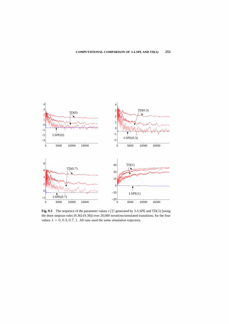
COMPUTATIONAL COMPARISON OF λ-LSPE AND TD(λ) 253
0 5000 10000 15000−20
−10
0
10
20
30
0 5000 10000 15000
−2
0
2
4
6
8
0 5000 10000 15000
−2
−1
0
1
2
3
4
0 5000 10000 15000
−3
−2
−1
0
1
2
3
4
LSPE(1)
TD(0.3)
LSPE(0.7)
LSPE(0)LSPE(0.3)
TD(1)
TD(0)
TD(0.7)
Fig. 9.3 The sequence of the parameter valuesr(2) generated byλ-LSPE and TD(λ) [usingthe three stepsize rules (9.36)-(9.38)] over 20,000 iterations/simulated transitions, for the fourvaluesλ = 0, 0.3, 0.7, 1. All runs used the same simulation trajectory.
Bibliography
1. A. Benveniste, M. Metivier, and P. Priouret,Adaptive Algorithms and StochasticApproximations,Springer-Verlag, N. Y., 1990.
2. D. P. Bertsekas, S. Ioffe, “Temporal Differences-Based Policy Iteration andApplications in Neuro-Dynamic Programming,”Lab. for Info. and DecisionSystems Report LIDS-P-2349,MIT, Cambridge, MA, 1996.
3. D. P. Bertsekas,Dynamic Programming and Optimal Control, 2nd edition,Athena Scientific, Belmont, MA, 2001.
4. D. P. Bertsekas, J. N. Tsitsiklis,Neuro-Dynamic Programming,Athena Scientific,Belmont, MA, 1996.
5. D. P. Bertsekas, J. N. Tsitsiklis, “Gradient Convergence in Gradient Methodswith Errors,”SIAM J. Optimization,vol. 10, pp. 627-642, 2000.
6. J. A. Boyan, “Technical Update: Least-Squares Temporal Difference Learning,”Machine Learning,vol. 49, pp. 1-15, 2002.
7. S. J. Bradtke, A. G. Barto,, “Linear Least-Squares Algorithms for TemporalDifference Learning,”Machine Learning,vol. 22, pp. 33-57, 1996.
8. P. D. Dayan, “The Convergence of TD(λ) for generalλ,” Machine Learning,vol. 8, pp. 341-362, 1992.
9. de D. P. Farias, B. Van Roy, “ On the Existence of Fixed Points for ApproximateValue Iteration and Temporal-Difference Learning ,”J. of Optimization Theoryand Applications,vol. 105, 2000.
10. L. Gurvits, L. J. Lin, and S. J. Hanson, “Incremental Learning of Evalua-tion Functions for Absorbing Markov Chains: New Methods and Theorems,”Preprint, 1994.
11. V. R. Konda, J. N. Tsitsiklis, “The Asymptotic Mean Squared Error of TemporalDifference Learning,” Unpublished Report,Lab. for Information and DecisionSystems,M.I.T., Cambridge, MA, 2003.
12. V. R. Konda,Actor-Critic Algorithms,Ph.D. Thesis, Dept. of Electrical Engi-neering and Computer Science, M.I.T., Cambridge, MA, 2002.
254
BIBLIOGRAPHY 255
13. Nedic, A., D. P. Bertsekas, “Least Squares Policy Evaluation Algorithms withLinear Function Approximation,”Discrete Event Dynamic Systems: Theory andApplications,Vol. 13, pp. 79-110, 2003.
14. F. Pineda, “Mean-Field Analysis for Batched TD(λ),” Neural Computation,pp.1403-1419, 1997.
15. M. L. Puterman,Markov Decision Processes,John Wiley Inc., New York, 1994.
16. R. S. Sutton, A. G. Barto,Reinforcement Learning,MIT Press, Cambridge, MA,1998.
17. R. S. Sutton, “Learning to Predict by the Methods of Temporal Differences,”Machine Learning,vol. 3, pp. 9-44, 1988.
18. B. Van Roy, “Learning and value Function Approximation in Complex DecisionProcessesw,” Ph.D. Thesis, Massachusetts Institute of Technology, May, 1998.
19. J. N. Tsitsiklis, B. Van Roy, “An Analysis of Temporal-Difference Learning withFunction Approximation,”IEEE Transactions on Automatic Control,vol. 42, pp.674-690, 1997.
10 Approximate DynamicProgramming for HighDimensional Resource AllocationProblems
WARREN B. POWELL and BENJAMIN VAN ROYPrinceton University Stanford University
Editor’s Summary: This chapter focuses on presenting a mathematical model fordynamic resource allocation problems and reviews computational methods includingapproximate dynamic programming that addresses them. Detailed examples andcomparisons are given to validate the advantages of solving these high-dimensionalcomplex problems using ADP.
10.1 INTRODUCTION
The allocation of human and physical resources over time is a fundamental problemthat is central to management science. For example, a freight transportation companymust manage personnel and equipment to move shipments in a timely manner in thepresence of a variety of dynamic information processes: customer demands, equip-ment failures, weather delays, and failures of execution. This is a high-dimensionalproblem since it involves a large number of resources, each of which must be trackedas it is affected by decisions and uncertainties.
In principle, problems of dynamic resource allocation can be treated as Markovdecision processes and solved using dynamic programming algorithms. Textbookdynamic programming algorithms – such as value iteration and policy iteration –typically require compute time and memory that grow exponentially in the number ofstate variables, the number of decision variables, and the number of random variablesthat affect the system in each time period. These three “curses of dimensionality”render such algorithms infeasible for problems of practical scale.
256
DYNAMIC RESOURCE ALLOCATION 257
In this paper, we focus on a formulation of dynamic resource allocation that was orig-inally motivated by problems in transportation but also captures problems arising ina variety of other settings. Practical problems formulated in terms of our model typ-ically involve thousands of state variables that describe current resources, thousandsof decision variables that determine what is to be done with each resource, and thou-sands of random variables that influence the state. These random variables captureuncertainties from a variety of sources, such as customer demands, the physical net-work, and characteristics of the people and equipment used to provide services (e.g.,equipment breakdowns and no-shows). Clearly, textbook dynamic programming al-gorithms are inapplicable, and solving such large-scale dynamic resource allocationproblems has proven to be a terrific challenge. In this chapter, we present examplesof approximate dynamic programming algorithms developed by the first author andcollaborators to address such problems. We also discuss the relation between thesealgorithms and ideas studied in the broader approximate dynamic literature (includ-ing “neuro-dynamic programming” and “reinforcement learning” methods) and themathematical programming literature.
This chapter is organized as follows. Section 10.2 presents a mathematical modelfor a broad class of resource allocation problems together with a simple illustrativeexample. Section 10.3 discusses how – in the context of our dynamic resourceallocation model – the three curses of dimensionality prevent application of textbookdynamic programming algorithms. In section 10.4, we present approximate dynamicprogramming algorithms designed for our model. We discuss in section 10.5 modelsand algorithms that have emerged from the field of mathematical programming, andthen review in section 10.6 relations to ideas that have evolved from within theapproximate dynamic programming literature. In section 10.7, we present someexperimental results.
10.2 DYNAMIC RESOURCE ALLOCATION
In this section, we present a formulation of dynamic resource allocation problems.After defining the formulation in section 10.2.1, we discuss in section 10.2.2 a simpleexample involving the management of a fleet of trucks. This example is a dramaticallysimplified version of a real trucking problem. However, it serves to illustrate howthe formulation maps to a practical context while avoiding the intricacies of trulyrealistic models (see, for example, [25, 28]).
10.2.1 Problem Formulation
We consider a system that evolves in discrete time overT periods. At each timet = 0, . . . , T , the state of the system is described by a state variableRt, taking theform:
a = The vector of attributes that describe a single resource.
A = The set of possible attributes.

258 ADP FOR HIGH DIMENSIONAL RESOURCE ALLOCATION PROBLEMS
Rta = The number of resources with attributea at timet.
Rt = (Rta)a∈A.
For our purposes, it is enough to describe a single resource class such as trucks orpeople or product, but more complex problems can exhibit multiple resource classes(tractors, trailers and drivers; pilots, aircraft and passengers). For these problems, wehave to define different resource classesCR. We then letAc be the attribute spacefor a resource classc ∈ CR, and we letRc
t be the vector of resources for classc. Ifwe letRt = (Rc
t)c∈CR then we can continue to letRt be our resource state.
At each timet = 0, . . . , T − 1, a decision is made on what to do with each resource.For any resource with attributea, there is a setDa of actions that can be applied tothe resource. The collection of actions applied at timet is represented by a decisionxt = (xtad)a∈A,d∈Da , wherextad is the number of resources with attributea thatactiond is applied to. In a transportation example involving the management ofequipment,a would capture the type and location of a piece of equipment and anaction might be to move the equipment from one location to another. Needless to say,each decision variablextad must be a nonnegative integer and the decision variablesmust satisfy flow conservation constraints:
∑
d∈Da
xtad = Rta ∀a ∈ A (10.1)
which we write compactly asAtxt = Rt, whereAt is a linear operator. Theremay also be additional constraints on the decision variable. We assume that theseconstraints are linear, taking the form
Utxt ≤ ut, (10.2)
whereUt is a linear operator mapping decisions toRnt for soment, so thatUtxt andut are elements of<nt .
The change that a decision induces on the stateRt is a linear function of the decision.We define a linear operator∆t by:
(∆txt)a = The number of resources that result in attributea given the decision vectorxt.
The vectorRt of resources that we can act on in time periodt is known as thepre-decision state vector. The resource vector after the resources have been acted onis given byRx
t = ∆txt. We refer toRxt as thepost-decisionstate vector, since it is
the state of our system immediately after decisions have been made.
There are also random shocks – new resources appear and existing resources can dis-appear randomly. This randomness is driven by a sequenceω1, . . . , ωT of indepen-dent identically distributed random variables. The random change during thetth pe-riod in the number of resources with attributea takes the formRa(Rx
t , ωt+1) for somefunctionRa. Note that this quantity is a function of both the random variableωt+1
DYNAMIC RESOURCE ALLOCATION 259
and the “post-decision” stateRxt = ∆txt. Let R(Rx
t , ωt+1) = (Ra(Rxt , ωt+1))a∈A.
The dynamics of our system are described by the simple equation:
Rt+1 = ∆txt + R(Rxt , ωt+1).
If our random changes are purely exogenous arrivals to the system (which do notdepend on the state of the system), we will writeR(ωt) as the exogenous arrivals tothe system during time intervalt.
At each time, we must select a feasible actionxt. For shorthand, we denote the feasi-ble set byXt(Rt) – this is the set of actionsxt with nonnegative integer componentsthat satisfy (10.1) and (10.2). Each actionxt is selected based only on the currentstateRt. Hence, we can think of decisions as being made by apolicy, which is afunctionXπ
t that maps each state to a feasible action:
xt = Xπt (Rt) ∈ Xt(Rt).
There are, of course, many different policies (functions) that we can use, so we letΠbe our family of policies (decision functions) that we can choose from.
The contribution (or reward) generated in eachtth period is a linear functionCtxt ofthe decisionxt. Here,Ct is a linear operator that gives the total contribution (if weare maximizing) of an action. Our objective is to select a policy that maximizes theexpected contribution over the horizon:
maxπ∈Π
E
[T−1∑t=0
CtXπt (Rt)
].
10.2.2 A Transportation Example
As an example to illustrate how our formulation might map to a real-world context,we discuss in this section a simplified model of a truckload motor carrier. For thesake of brevity, we will only discuss at a very high level how elements of the modelmight be used to capture features of the application.
Consider the management ofN trucks moving amongL cities overT time periods.Loads materialize at various cities, and each load is tagged with a destination. Forthe sake of simplicity, we assume that the only source of uncertainty is in demand(i.e., the loads that materialize in various cities).
We now discuss how one might formulate the problem in terms of our mathematicalmodel. The attributea specifies either that the resource is residing in a particularcity, or that the resource is travelling, in which case the attributea further specifiesthe next city where the resource will arrive and the time until arrival.
The random variableR(Rxt , ωt+1) captures new loads entering the system. The
number of loads that materialize at each city in a given time period is independentof the numbers at other cities, and these arrivals are independent and identically

260 ADP FOR HIGH DIMENSIONAL RESOURCE ALLOCATION PROBLEMS
distributed over time. Note that, in this special case,R only depends onωt+1 andnotRx
t .
The set of possible actionsDa that can be applied to a resource depends on itscurrent attribute. For example, a driver in one location can typically be assignedto move loads that are not too far away. Furthermore, the attribute vector mightcapture other characteristics of a driver that limit what a driver can do. For example,a Canadian-based driver in the United States can only accept a load that returns himto Canada.
Some additional constraints are placed on the choice of the aggregate collection ofactionsxt. The flow conservation constraint (10.1) ensures that we only act on thetrucks and loads that are available. Further requirements are that a load can onlymove if it is on a truck and that a truck can only carry a single load at a time. Theserequirements can be represented as a linear constraintUtxt ≤ ut for appropriatelydefinedUt andut.
The operator∆t captures how resources migrate in the system and how loads leavethe system as consequences of decisions. Each load generates a contribution upondelivery. The contribution is a decreasing function of the time taken to serve theload, as specified by its attributea. The net contribution in a time period can berepresented as a linear functionCtxt of xt.
10.3 THE CURSES OF DIMENSIONALITY
The problem of dynamic resource allocation can – in principle – be addressed viadynamic programming. In particular, value functionsV0, . . . , VT are computed bysetting
VT (RT ) = 0, (10.3)
and applying the recursion
Vt(Rt) = maxx∈Xt(Rt)
(Ctx + Et
[Vt+1
(Rx
t + R(Rxt , ωt+1)
)]), (10.4)
where the expectation is taken over possible outcomes ofRt+1. We use the subscriptwith the expectation operator to indicate the conditioning information. In particular,for anyt, Et denotes a conditional expectation, conditioned onω1, . . . , ωt (if t = 0,this translates to an expectation with respect to the prior distribution). Optimaldecisionsxt can then be generated according to
xt ∈ argmaxx∈Xt(Rt)
(Ctx + Et
[Vt+1
(Rx
t + R(Rxt , ωt+1)
)]).
Three computational obstacles prevent use of this textbook approach when dealingwith problems of practical scale. First, the number of possible state vectorsRt

ALGORITHMS FOR DYNAMIC RESOURCE ALLOCATION 261
grows very quickly with the number|A| of possible attributes, making computationof Vt(Rt) for every possibleRt unmanageable. Second, exact computation of theexpectation is infeasible because the number of possible outcomes ofωt+1 typicallybecomes enormous as|A| grows. Finally, finding an optimal decisionxt fromthe discrete spaceXt generally requires an exhaustive search overXt. This spaceonce again grows extremely quickly as|A| grows, rendering an exhaustive searchinfeasible. We refer to these three obstacles as the three “curses of dimensionality.”
We note that some authors have studied formulations similar to what we have pre-sented and solved problem instances using exact dynamic programming techniques([1, 16]). However, the problems instances treated involve very few variables – a farstretch from the scale of real transportation systems.
10.4 ALGORITHMS FOR DYNAMIC RESOURCE ALLOCATION
In this section, we present algorithms developed by the first author with collaboratorsto address large-scale dynamic resource allocation problems of the type presented insection 10.2. These algorithms incorporate several ideas, one of which involves areformulation of dynamic programming equations in terms of a “post-decision state.”We discuss this reformulation in section 10.4.1. The algorithms approximate a valuefunction. This requires design of an approximation architecture and execution ofalgorithms that fit the approximation architecture to the value function. Two particularapproximation architectures that have been successfully applied to transportationproblems are discussed in section 10.4.2. In section 10.4.3 we present algorithmsused to fit these approximation architectures.
10.4.1 The Post-Decision State
Earlier we introduced the notion of a “post-decision state”Rxt = Rt + ∆txt. This
is the state of the system after being modified by the actionxt taken at timet butbefore being affected by the random variableRt+1. Let V x
t (Rxt ) be the maximal
expected sum of contributions to be received from decisionsxt+1, . . . , xT−1, giventhe post-decision stateRx
t , so that
V xt (Rx
t ) = Et
[Vt
(Rx
t + R(Rxt , ωt+1)
)].
It is easy to show thatV xt can be computed by setting
V xT−1(R
xT−1) = 0, (10.5)
and applying the recursion
V xt (Rx
t ) = Et
[max
x∈Xt+1(Rxt +R(Rx
t ,ωt+1))
(Ct+1x + V x
t+1 (∆t+1x))]
. (10.6)
262 ADP FOR HIGH DIMENSIONAL RESOURCE ALLOCATION PROBLEMS
Further, optimal decisions can be generated according to
xt ∈ argmaxx∈Xt(Rt)
(Ctx + V xt (∆t+1x)) .
The new recursion is similar to the standard dynamic programming recursion (10.4)used for computingVt. An important difference, however, is that this new recursion(10.6) involves the expectation of a maximum whereas (10.4) requires computing themaximum of an expectation. This difference in the form of (10.6) can be critical foruse of simulation-based methods, as we will discuss in the section 10.4.3.
10.4.2 Approximation Architectures
Our approach to high-dimensional dynamic resource allocation problems involvesapproximating each value functionV x
t using anapproximation architecture; thatis, a family of functionsV x parameterized by a vectorv of real values, so thateachV x(·, v) is a function mapping states to real values. Approximation of thevalue function involves choosing an appropriate approximation architecture and thencomputing parametersvt so thatV x(·, vt) ≈ V x
t . Given such an approximation,suboptimal decisionsxt can be generated according to
xt ∈ argmaxx∈Xt(Rt)
(Ctx + V x(∆tx, vt)
). (10.7)
When choosing an approximation architecture, one must strike a balance betweencomputational efficiency and performance of the resulting policy. Some approxima-tion architectures may amplify computational challenges. For example, a second orthird order polynomial approximation toV x
t may turn the maximization problem in(10.7) into a very difficult integer program. On the other hand, specially structuredapproximation architectures such as those we will discuss next may sometimes leadto computationally tractable integer programming problems; e.g., in some cases themaximization problem in (10.7) may become an easily solved network optimizationproblem.
Two classes of approximation architectures have been successfully applied to a varietyof problems in transportation operations. These are linear (in the state variable)architectures:
V x(Rt, vt) =∑
a∈AvtaRta, (10.8)
and separable concave architectures:
V x(Rt, vt) =∑
a∈A
bRtac∑
i=1
vtai + (Rta − bRtac)vtadRtae
, (10.9)

ALGORITHMS FOR DYNAMIC RESOURCE ALLOCATION 263
wherevtai ≥ vtaj for all t, a, andi ≤ j. In the linear case, the parameter vectortakes the formvt = (vta)a∈A, whereas in the separable concave case, we havevt = (vtai)a∈A,i∈1,Rmax
ta , whereRmaxta is an upper bound on the values thatRx
ta cantake on. Though states are integer-valued, these approximation architectures assignvalues to all elements of the positive orthant. This is required to make the optimizationproblem (10.7) amenable to available software for solving integer programs. Notethat the separable concave architecture can realize any separable concave functionon the integers. Each non-integer point is assigned a value corresponding to alinear interpolation. Each of the two architectures offers specific advantages anddisadvantages, as we now discuss.
Not surprisingly, linear approximations are the easiest to work with. They willwork well when the value function is approximately linear over the range of interest,and also for discrete routing and scheduling problems whereRta ∈ 0, 1. If theone-period problem,
xt ∈ argmaxx∈Xt(Rt)
Ctx,
exhibits structure that facilitates efficient solution (for example, network or near-network structure) a linear approximation to the value function will retain this struc-ture in (10.7). Additionally, linear approximations offer computational advantageswith regards to algorithms for computing appropriate parametersvt. Linear approxi-mations should generally be tried before other, more complex strategies, but they cansometimes work poorly. In such cases, one must move on to a richer approximationarchitecture.
For some problems, the value function is nonlinear but concave, and separableconcave functions have proven to offer useful approximations. Although they aretypically harder to work with than linear approximations, the decision optimizationproblem (10.7) often still retains network or near-network structure if the one-periodproblem exhibits such structure. For example, in certain problems involving man-agement of homogeneous resources, the optimization problem (10.7) exhibits purenetwork structure so that solution of the linear programming relaxation naturallyproduces integer solutions (see, for example, [10]). In more realistic problems, re-sources are heterogeneous. The resulting optimization problems do not generallyexhibit pure network structure. Nevertheless, solution of the linear programmingrelaxation results in integer solutions the vast majority of the time, and non-integersolutions are often easy to resolve.
10.4.3 Algorithms
In this section, we describe algorithms for computing parameter values to fit linearand separable concave approximations to the value function. These algorithms arerepresentative of ideas developed by the first author and collaborators to tacklelarge-scale problems in transportation and logistics. In order to deliver a briefand accessible exposition, we have chosen to present relatively simple versions of

264 ADP FOR HIGH DIMENSIONAL RESOURCE ALLOCATION PROBLEMS
the algorithms. More complicated variations that improve on execution time andmemory requirements can be found in ([28, 10, 33],and [26]). Such improvementsare often critical for practical application to realistic large-scale problems.
The algorithms we will present are iterative and integrate integer programming,stochastic approximation, and function approximation. Each iteration involves anindependent simulated sequenceω1, . . . , ωT and adjusts the parametersv0, . . . , vT−2
by small amounts. The algorithms for linear and separable concave architectures areidentical except for one step, so we describe them as one algorithm and only delineatethe two cases when required. In stating the algorithm, we will use some new notation.For eacha, a ∈ A, let δa
a = 1 andδaa = 0 for a 6= a (note that this can be thought
of as a Dirac delta function). Also, letδa = (δaa)a∈A. The algorithm takes as a
parameter a step sizeγ, which is generally chosen to be a small positive scalar. Leteach element ofvt be initialized to0. Each iteration of the algorithm executes thefollowing steps:
1. Generate random sequence.Sample the random sequenceω1, . . . , ωT .
2. Simulate state trajectory. For t = 0, . . . , T − 1, let
xt ∈ argmaxx∈Xt(Rt)
(Ctx + V x(∆tx, vt)
)
Rxt = ∆txt
Rt+1 = Rxt + R(Rx
t , ωt+1).
3. Estimate gradient. For t = 0, . . . , T − 2 anda ∈ A such thatRxta < Rmax
ta ,let
qt = Ct+1xt+1 + V x(Rxt+1, vt+1)
Rx+ta = Rx
t + δa
q+ta = max
x∈Xt+1(Rxt +δa+R(Rx
t +δa,ωt+1))
(Ct+1x + V x(∆t+1x, vt+1)
)
dta = q+ta − qt.
4. Update approximation architecture parameters.For t = 0, . . . , T − 2 anda ∈ A such thatRx
ta < Rmaxta , apply
(a) Linear case.
vta := (1− γ)vta + γdta.
(b) Separable concave case.For the slope elementi = (Rxta + 1):
vtai := (1− γ)vtai + γdta,

ALGORITHMS FOR DYNAMIC RESOURCE ALLOCATION 265
which may produce a nonconcave function. Restore concavity accordingto:
if vta(Rxta+1) > vtaRx
ta:
vtaRxta
:=vtaRx
ta+vta(Rx
ta+1)
2
vta(Rxta+1) :=
vtaRxta
+vta(Rxta+1)
2
if vta(Rxta+1) < vta(Rx
ta+2) :vta(Rx
ta+1) :=vta(Rx
ta+1)+vta(Rxta+2)
2
vta(Rxta+1) :=
vta(Rxta+1)+vta(Rx
ta+2)
2 .
(10.10)
Let us now provide an interpretation of the algorithm. Each sampled sequenceω1, . . . , ωT is used in Step 2 to generate a sample trajectory of statesR0, Rx
0 , . . .,RT−1, Rx
T−1, RT . In addition to the random sequence, this state trajectory isinfluenced by decisionsx0, . . . , xT−1. As the state trajectory is generated, thesedecisions are selected to optimize an estimate of future contribution. This estimateis taken to be the sumCtxt + V x(Rt + ∆txt, vt) of immediate contribution andan approximation of subsequent contribution given byV x(·, vt). Implicit in thestatement of our algorithm is that we have access to a subroutine for optimizing thisestimate overx ∈ Xt(Rt). The optimization problem is an integer program, andas discussed in the previous section, for applications in transportation and logistics,it often exhibits network or near-network structure. This facilitates use of availablesoftware for integer programming. Though there are no theoretical guarantees whenthe problem does not exhibit pure network structure, this approach appears to workwell in practice.
For each attributea ∈ A and post-decision stateRxt , Step 3 estimates how availability
of an additional unit of a resource with attributea would have impacted the predictionof future contribution. The difference is denoted bydta. Step 4 is a stochasticapproximation iteration that tunes the gradient of the approximationV x(Rx
t , vt) withrespect toRx
t to be closer to the estimated gradientdt.
In the case of a separable concave approximation, an extra step after the tuningprojects the approximation back into the space of concave functions, if the tuningstep destroys concavity. Note that we cannot even allow intermediate functionalapproximations to be nonconcave because of the complexities this would introduceto the problem of optimizing overx ∈ Xt(Rt). For a discussion of methods formaintaining concavity, see [11, 37, 27].
We mentioned earlier that reformulation of the dynamic programming recursion interms of a post-decision state could be critical to the use of simulation-based methods.Let us now discuss how this relates to the above algorithm. One could imaginedeveloping an analogous algorithm to approximate the pre-decision value functionVt(Rt) using an approximation architectureV (Rt, vt). Again, we would generatea random sequence, simulate the corresponding state trajectory, estimate gradientsof predicted contribution, and update the approximation architecture accordingly.However, a difficulty arises in the Step 3, as we now explain.

266 ADP FOR HIGH DIMENSIONAL RESOURCE ALLOCATION PROBLEMS
In Step 3,qt can be viewed as a sample estimate of
Et
[max
x∈Xt+1(Rxt +R(Rx
t ,ωt+1))
(Ct+1x + V x(∆t+1x, vt)
)]
. (10.11)
It is easy to see thatqt is an unbiased estimate of this expectation, and this is important,since the stochastic approximation updates essentially average these estimates tobetter estimate the expectation.
Suppose now that we wish to adapt the algorithm so that it works with a pre-decisionvalue functionV (Rt, vt). Then, in Step 3, we would want to generate an unbiasedestimate of
maxx∈Xt(Rt)
(Ctx + Et
[V (Rt + ∆tx + R(Rt + ∆tx, ωt+1), vt)
]), (10.12)
based on a sampled value ofωt+1. In general, this is not possible. Unlike theexpectation of the maximum (10.11), there is no simple way of generating an unbiasedestimate of the maximum of an expectation (10.12) based on a single sample ofωt+1.An exception to this, however, arises in the case of a linear approximation architectureif R depends onRt instead ofRx
t . In this event, we have
maxx∈Xt(Rt)
(Ctx + Et
[V
(∆tx + R(Rt, ωt+1), vt
)])
= maxx∈Xt(Rt)
(Ctx + V (∆tx, vt)
)+ Et
[V
(R(Rt, ωt+1), vt
)].
Clearly, an unbiased estimate can be generated by maximizing the first term on theright hand side and addingV (R(Rt, ωt+1), vt) generated from a single sampleωt+1.On the other hand, when the approximation architecture is nonlinear orR dependsRx
t , an unbiased estimate can no longer be generated based on a single sample.
10.5 MATHEMATICAL PROGRAMMING
The problem formulation and algorithms we have presented evolved from a line ofwork on solution methods for large-scale problems in transportation and logistics.As of this writing, this field is dominated by algorithms developed within the mathe-matical programming community for handling high-dimensional resource allocationproblems. We briefly review a simple deterministic model (for which there is a vastarray of algorithms) and then introduce two competing themes that have emergedfrom within this community for introducing uncertainty.

MATHEMATICAL PROGRAMMING 267
10.5.1 Deterministic mathematical programming
In the field of transportation and logistics, the most common modelling and algo-rithmic strategy is to formulate the problem deterministically and then use classicalmath programming algorithms to solve the resulting model. For example, consider adeterministic version of the problem we introduced in section 10.2.1 resulting fromsettingR(Rx
t , ωt+1) = Rt+1 for a deterministic sequenceR1, . . . , RT . This wouldlead to a deterministic optimization problem:
maxx0,...,xT−1
T−1∑t=0
Ctxt (10.13)
subject to, fort = 0, . . . , T − 1:
Atxt = Rt (10.14)
Utxt ≤ ut (10.15)
Rt+1 = ∆txt + Rt+1 (10.16)
xt ≥ 0 and integer-valued (10.17)
As with our stochastic formulation from section 10.2.1, Eq. (10.14) typically repre-sents flow conservation. Eqs. (10.15) and (10.17) impose upper and lower boundson the flow. Eq. (10.16) captures the state dynamics.
Deterministic problems like the one we have formulated often result in large, timestaged linear integer programs. These can sometimes be solved effectively. However,they completely ignore uncertainty and some of the more complex dynamics that canarise in real-world settings.
10.5.2 Stochastic Programming
The most common approach for modelling resource allocation problems in practiceis to formulate the problem deterministically and apply mathematical programmingalgorithms developed for this setting. When uncertainty is introduced into mathe-matical programming, we find ourselves in a subfield calledstochastic programming.In a sense, Markov decision processes might be viewed as an extension of stochasticsystems models to incorporate optimization, while stochastic programming might beviewed as an extension of (deterministic) mathematical programming to incorporateuncertainty.
Two algorithmic strategies have emerged from the stochastic programming commu-nity. The first, covered in section 10.5.2.1, uses an explicit representation of decisionsin the future for each of a finite set of scenarios. This approach is fundamentallydifferent approach from dynamic programming. The second strategy, called Bendersdecomposition (section 10.5.2.2) uses a method for approximating the downstreamimpact of decisions. This is much closer in spirit to dynamic programming.

268 ADP FOR HIGH DIMENSIONAL RESOURCE ALLOCATION PROBLEMS
10.5.2.1 Scenario methodsThe oldest strategy to solving linear programs underuncertainty is stochastic programming using scenario methods. The roots of thisapproach date to the work by Dantzig ([9]), but the earliest serious investigationof stochastic programs were primarily due to Wets ([48, 49, 43, 50]). For modernreviews of this field, see [5, 14, 15, 32]).
As an example, let us formulate a scenario-based stochastic program to solve aproblem similar to that posed by our model of section 10.2.1. Let uncertainty berepresented in terms of a trajectory of random outcomesω = (ω1, . . . , ωT ). LetΩ bethe set of possible “scenarios”ω, and letp(ω) be the probability that eachω ∈ Ω willoccur. The random impact on resources at timet is assumed to take the formRt(ω).Using this representation of uncertainty, consider solving the following optimizationproblem:
maxx0,xt(ω)|t=1,...,T−1,ω∈Ω
C0x0 +∑
ω∈Ω
p(ω)T−1∑t=1
Ctxt(ω) (10.18)
subject to the following first stage constraints forω ∈ Ω:
A0x0 = R0 (10.19)
U0x0 ≤ u0 (10.20)
R1(ω) = ∆0x0 + R1(ω) (10.21)
x0 ≥ 0 and integer-valued (10.22)
and the subsequent stage constraints, fort = 1, . . . , T − 1 andω ∈ Ω:
Atxt(ω) = Rt(ω) (10.23)
Utxt(ω) ≤ ut (10.24)
Rt+1(ω) = ∆txt(ω) + Rt+1(ω) (10.25)
xt(ω) ≥ 0 and integer-valued (10.26)
This formulation allows us to make a different set of decisions for each outcome,which means we are allowing a decision to “see” into the future. To prevent thisbehavior, we incorporate an additional constraint for eacht = 1, . . . , T − 1 and pairof scenariosω, ω′ ∈ Ω for which (ω1, . . . , ωt) = (ω′1, . . . , ω
′t):
xt(ω) = xt(ω′) (10.27)
The constraints (10.27) are callednonanticipativity constraints.
We note that there is no explicit use of a state variable. This approach has provenuseful in the financial services sector where random processes (e.g. interest rates,currency fluctuations, stock prices) can be correlated in a very complex way. Thistechnique is widely used in financial asset allocation problems for designing low-risk
MATHEMATICAL PROGRAMMING 269
portfolios ([21, 18]), and a variety of specialized algorithms have been designed tohelp solve these problems ([17, 20, 19]).
The optimization problem represented by Eqs. (10.18)-(10.27) requires determin-ing all decisions over all scenarios (over all time periods) at the same time. Notsurprisingly, the resulting optimization problem ismuchlarger than its deterministiccounterpart. In addition, the formulation typically destroys integrality properties thatmight exist in the original problem. The solution of stochastic integer programs isan emerging area of research (see [31] for a thorough review of this field). This ap-proach is generally not computationally tractable in the context of large scale resourceallocation.
10.5.2.2 Benders DecompositionAn alternative strategy, which exploits the struc-ture of linear programs, is to replace the second term on the right hand side of Eq.(10.18) with a series of cuts that captures the structure of this function. We discussthis approach in the context of a two-stage problem – that is, the case ofT = 2. Theidea is to iteratively solve a sequence of “master problems” of the form:
maxx0,z
C0x0 + z (10.28)
subject to the first stage constraints (10.19)-(10.22) and the constraints:
z − βix0 ≤ αi, ∀ i = 1, ..., n (10.29)
whereβi andαi are generated by solving the dual of a second stage problem:
maxx1(ω)
C1x1(ω) (10.30)
subject to constraints (10.23)-(10.26). The second stage is solved for a singleω ∈ Ω,so the problem is no larger than a one-period deterministic problem. After solvingthe second stage problem for a single scenario, the dual information is used to updatethe cuts in Eq. (10.29). There are different strategies for creating and updating cuts.The “L-shaped decomposition algorithm” ([42]) solves two-stage problems with afinite set of scenarios. In one of the major breakthroughs in the field, [13] describethe “stochastic decomposition” algorithm that generalizes the L-shaped algorithmfor problems with an infinite number of scenarios. [30] and [6] present variationsof Benders for multistage problems. Figure 10.1 provides a sketch of the CUPPSalgorithm in [6] which is basically a generalization of the L-shaped algorithm formultistage problems.
The appeal of Benders decomposition is seen by simply comparing the problemof solving Eq. (10.28) along with Eq. (10.30) to the challenge of solving Eq.(10.18). Benders decomposition exploits the structure of a linear program, howeverthe rate of convergence remains an open question. [27], for example, found thatBenders algorithm could require hundreds of iterations before it outperformed a

270 ADP FOR HIGH DIMENSIONAL RESOURCE ALLOCATION PROBLEMS
Step 1. Solve the followingmaster problem:
xn0 ∈ arg maxC0x + z : A0x0 = R0, z − βkx ≤ αk, k = 1, . . . , n− 1, x ≥ 0
Step 2. Sampleωn ∈ Ω and solve the following dualsubproblem:
v(xn0 , ωn) ∈ arg min(R1(ωn) + ∆0xn
0 )T v : AT1 v ≥ C1
Augment the set of dual vertices by:
Vn = Vn−1⋃v(xn
0 , ωn)
Step 3. Set:
vn(ω) ∈ arg min(R1(ω) + ∆0xn0 )v : v ∈ Vn for all ω ∈ Ω
Step 4. Construct the coefficients of thenth cut to be added to the master problem by:
αn + βnx0 ≡∑
ω∈Ω
p(ω)(R1(ω) + ∆0x0
)Tvn(ω)
Fig. 10.1 Sketch of the CUPPS algorithm
simple deterministic approximation even for relatively small problems (the rate ofconvergence slows as the problem size increases).
Benders can be used for multistage problems by simply stepping forward throughtime, a technique that is sometimes referred to as nested Benders decomposition (see[23] for an application in an energy setting and [2] for an application to reservoiroptimization). The basic strategy is identical to that used in approximate dynamicprogramming.
For an analysis of the convergence of these techniques see [30] and [6].
10.6 APPROXIMATE DYNAMIC PROGRAMMING
The algorithms we have presented emerged from a thread of research that grew toa large extent independently from the broader approximate dynamic programmingliterature – which includes, for example, work under the guise of “neuro-dynamicprogramming,” “reinforcement learning,” and “heuristic dynamic programming.” Werefer the reader to [4, 35, 40] for surveys of this literature. There are a number ofideas in common between the algorithm we have presented and those proposed inthis approximate dynamic programming literature. In this section, we discuss thesesimilarities and also some notable differences.
Like algorithms from the broader approximate dynamic literature, the algorithmpresented in section 10.4 approximates a dynamic programming value function foruse in decision-making. Another striking commonality is the use of simulated statetrajectories and stochastic approximation updates. In this respect, the algorithmof section 10.4 is closely related to temporal-difference learning ([34]), Q-learning
APPROXIMATE DYNAMIC PROGRAMMING 271
([44] and [45]), and SARSA ([29]). Some work in the reinforcement learningliterature highlights the importance of simulated state trajectories towards reducingapproximation error ([36] and [39]). Perhaps this phenomenon has also contributedto the empirical success in transportation of algorithms like that of section 10.4.
The formulation of dynamic programs around the pre-decision state is the most stan-dard treatment in textbooks, though even Bellman’s original treatment of dynamicprogramming ([3], p. 142) included an example of a dynamic programming recursionin terms of a post-decision state. In our context, such a reformulation of the dynamicprogramming recursion becomes necessary to enable computation of unbiased esti-mates of the right hand side via simulation. Such a reformulation is employed for thesame reason by Q-learning and SARSA. One interesting difference, though, is thatthe post-decision state used by Q-learning and SARSA is taken to be the state-actionpair – in our context, this would be(Rt, xt). The algorithm we have presented, onthe other hand, makes use of a more parsimonious representationRx
t = Rt + ∆txt
of the post-decision state. This is possible because of special structure associatedwith our problem formulation, which makesRx
t a sufficient statistic for predictingfuture contribution. Since Q-learning is designed for more general Markov decisionprocesses that do not exhibit such structure, it can not make use of such a sufficientstatistic. The idea of using a parsimonious sufficient statistic has also been proposedin an application of approximate dynamic programming to inventory management([41]). The use of the post-decision state variable is implicit in the work of [24] and[7] for a stochastic fleet management problem, and is explicit in [10] for the sameproblem class, and [22] and [33] in other problem classes.
Another significant difference in the algorithm of section 10.4 is that the updates adaptthe derivative of the value function with respect to state, whereas most algorithmsin the approximate dynamic programming literature adapt the values themselves.Clearly, it is the derivative of the value function that matters when it comes todecision-making, since the value function is only used to compare relative valuesamong states. An interesting issue to explore may be whether there are fundamentaladvantages to adapting derivatives rather than values. Though the idea of adaptingderivatives has not been a focus of the approximate dynamic programming literature,it has received some attention. For example, this idea has been promoted by Werbos,who proposed a number of algorithms with this objective in mind ([46] and [47]).
An important departure from the broader approximate dynamic programming litera-ture is in the use of integer programming methods to solve the decision optimizationproblem
maxx∈Xt(Rt)
(Ct+1x + V x(∆t+1x, vt+1)
).
This approach has been successfully applied to problems involving thousands of deci-sion variables. Though there is some work in the approximate dynamic programmingliterature on approaches for dealing with high-dimensional decision spaces (see, e.g.,[4, 8, 12]), to our knowledge, no other applications of approximate dynamic pro-gramming have dealt with such large numbers of decision variables.

272 ADP FOR HIGH DIMENSIONAL RESOURCE ALLOCATION PROBLEMS
The use of separable linear and concave approximations facilitate the use of integerprogramming methods to optimize decisions. Though separable approximators havebeen used regularly in the approximate dynamic programming literature (see, e.g.,[36]), there has not been a practice of restricting to linear or concave functions, andtheir use has not been motivated by a need to structure the decision optimizationproblem. The separable linear or concave structure is important – if more generalnonlinear approximations were used this would likely destroy integrality propertiesof underlying linear programs. The result would be a decision optimization problemthat could not be handled effectively by integer programming methods.
Finally, it is worth noting that the scale of problems tackled by the first author and col-laborators far exceeds most other applications of approximate dynamic programmingreported in the literature. In particular, there are typically thousands of state variablesand thousands of decision variables. For problems of such enormous scale, it be-comes important to use methods for which compute time and memory requirementsgrow slowly with the number of state variables. In this respect, separable approx-imation architectures are advantageous because the number of parameters involvedgrows linearly in the number of state variables.
10.7 EXPERIMENTAL COMPARISONS
The techniques described in this chapter have evolved in the context of solving anarray of very large-scale resource allocation problems. One of the challenges that wealways face in the field of approximate dynamic programming is evaluating how wellour techniques work. Bounds can be useful, but tend to be quite loose in practice.
For our problem class, we can report on two types of experiments. The first focuses ontwo-stage problems (make a decision in the first stage, see information in the secondstage, make a second decision, stop), for which computationally tractable, provablyconvergent algorithms already exist using the principle of Benders decomposition(which we reviewed in section 10.5.2.2). The second set of experiments look atmultiperiod problems, and compare against rolling horizon approximations that usedeterministic forecasts of the future.
Figure 10.2 shows comparisons of three variations of Benders against a variation ofthe concave, separable approximation method (described in section 10.4.3) calledthe SPAR algorithm (see [27]). The algorithms were run on four sets of problem ofincreasing size (10, 25, 50 and 100 locations). The execution times are comparable(although the “L-shaped” algorithm is much slower than the others). But the resultssuggest that Benders exhibits higher errors after the same number of iterations, andthat the error increases dramatically with problem size, whereas the SPAR algorithmactually improves. This is capturing the observation that in practice, large problemsare reasonably approximated using separable approximations.
Benders decomposition can be run on multiperiod problems as well, but the rate ofconvergence appears to become prohibitively slow. The best competition comes fromthe standard engineering practice of solving sequences of deterministic approxima-

EXPERIMENTAL COMPARISONS 273
Fig. 10.2 The quality of the solution produced by variations of Benders and separable, concave ap-proximations (SPAR) expressed as a percent of the optimal solution found using L-shaped decomposition.Based on results from [27].
tions using a rolling horizon procedure. [38] reports on comparisons using linearand piecewise linear, concave value function approximations against a deterministic,rolling horizon procedure. Table 10.1 summarizes one set of experiments that consid-ered problems with 10, 20 and 40 locations. Each cell in this table gives the averageobjective function for each method divided by the average of all the posterior boundsobtained by calculating the (outcome-dependent) optimal solutions for each of the100 sample realizations tested. This set of experiments focused on an applicationwith different equipment types (such as box cars) which can be described purelybased on the type of equipment and their location. It is possible to substitute differentequipment types for the same order (at a cost), as well as substituting equipmentof the same type from different locations. Separable concave value functions areestimated for each location and equipment type, which would suggest a significantpotential for error. Just the same, separable concave approximations work quite wellagainst the linear approximations (which works the worst) and the rolling horizonprocedure.
As of this writing, we do not know exactly how well these methods work on general,multistage problems given the lack of effective, computationally tractable compet-ing algorithms. There are many unanswered questions, but there has been enoughprogress to suggest that this is a promising line of investigation for this problem class.
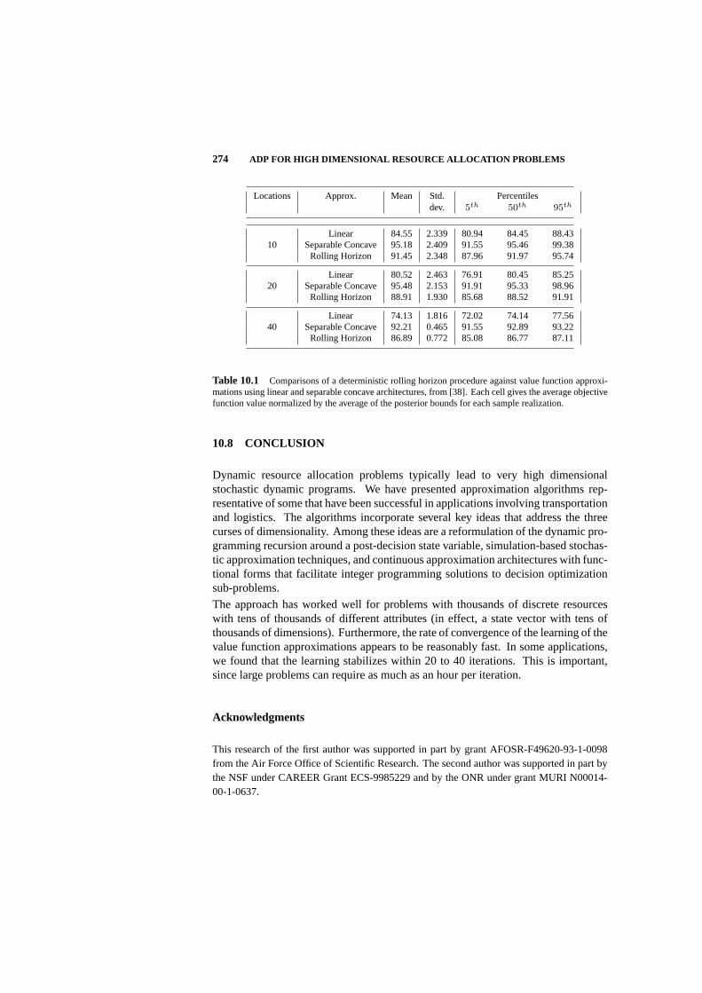
274 ADP FOR HIGH DIMENSIONAL RESOURCE ALLOCATION PROBLEMS
Locations Approx. Mean Std. Percentilesdev. 5th 50th 95th
Linear 84.55 2.339 80.94 84.45 88.4310 Separable Concave 95.18 2.409 91.55 95.46 99.38
Rolling Horizon 91.45 2.348 87.96 91.97 95.74
Linear 80.52 2.463 76.91 80.45 85.2520 Separable Concave 95.48 2.153 91.91 95.33 98.96
Rolling Horizon 88.91 1.930 85.68 88.52 91.91
Linear 74.13 1.816 72.02 74.14 77.5640 Separable Concave 92.21 0.465 91.55 92.89 93.22
Rolling Horizon 86.89 0.772 85.08 86.77 87.11
Table 10.1 Comparisons of a deterministic rolling horizon procedure against value function approxi-mations using linear and separable concave architectures, from [38]. Each cell gives the average objectivefunction value normalized by the average of the posterior bounds for each sample realization.
10.8 CONCLUSION
Dynamic resource allocation problems typically lead to very high dimensionalstochastic dynamic programs. We have presented approximation algorithms rep-resentative of some that have been successful in applications involving transportationand logistics. The algorithms incorporate several key ideas that address the threecurses of dimensionality. Among these ideas are a reformulation of the dynamic pro-gramming recursion around a post-decision state variable, simulation-based stochas-tic approximation techniques, and continuous approximation architectures with func-tional forms that facilitate integer programming solutions to decision optimizationsub-problems.
The approach has worked well for problems with thousands of discrete resourceswith tens of thousands of different attributes (in effect, a state vector with tens ofthousands of dimensions). Furthermore, the rate of convergence of the learning of thevalue function approximations appears to be reasonably fast. In some applications,we found that the learning stabilizes within 20 to 40 iterations. This is important,since large problems can require as much as an hour per iteration.
Acknowledgments
This research of the first author was supported in part by grant AFOSR-F49620-93-1-0098from the Air Force Office of Scientific Research. The second author was supported in part bythe NSF under CAREER Grant ECS-9985229 and by the ONR under grant MURI N00014-00-1-0637.

Bibliography
1. J. Alden, R. Smith, “Rolling horizon procedures in nonhomogeneous markovdecision processes,”Operations Research,vol. 40, no. 2, pp. S183-S194, 1992.
2. T. W. Archibald, C. S. Buchanan, K. I. M. McKinnon, and L. C. Thomas, “Nestedbenders decomposition and dynamic programming for reservoir optimisation,”J. Oper. Res. Soc.,vol. 50, pp. 468-479, 1999.
3. R. Bellman,Dynamic Programming,Princeton University Press, Princeton,1957.
4. D. Bertsekas, J. Tsitsiklis,Neuro-Dynamic Programming,Athena Scientific,Belmont, MA, 1996.
5. J. Birge, F. Louveaux,Introduction to Stochastic Programming,Springer-Verlag,New York, 1997.
6. Z.-L. Chen, W. Powell, “A convergent cutting-plane and partial-sampling algo-rithm for multistage linear programs with recourse,”Journal of OptimizationTheory and Applications,vol. 103(3), pp. 497-524, 1999.
7. R. Cheung, W. B. Powell, “An algorithm for multistage dynamic networkswith random arc capacities, with an application to dynamic fleet management,”Operations Research,vol. 44(6), pp. 951-963, 1996.
8. R. Crites, A. Barto, “Elevator group control using multiple reinforcement learn-ing agents,” Technical report, 1994.
9. G. Dantzig, A. Ferguson, “The allocation of aircrafts to routes: An exampleof linear programming under uncertain demand,”Management Science,vol. 3,pp. 45-73, 1956.
10. G. Godfrey, W. B. Powell, “An adaptive, dynamic programming algorithm forstochastic resource allocation problems I: Single period travel times,”Trans-portation Science,vol. 36(1), pp. 21-39, 2002.
11. G. A. Godfrey, W. B. Powell, “An adaptive, distribution-free approximation forthe newsvendor problem with censored demands, with applications to inventory
275
276 BIBLIOGRAPHY
and distribution problems,”Management Science,vol. 47(8), pp. 1101-1112,2001.
12. C. Guestrin, D. Koller, and R. Parr, “Efficient solution algorithms for factoredMDPs,” Technical report, 2003.
13. J. Higle, S. Sen, “Stochastic decomposition: An algorithm for two stage lin-ear programs with recourse,”Mathematics of Operations Research,vol. 16(3),pp. 650-669, 1991.
14. G. Infanger,Planning under Uncertainty: Solving Large-scale Stochastic LinearPrograms,The Scientific Press Series, Boyd & Fraser, New York, 1994.
15. P. Kall, S. Wallace,Stochastic Programming,John Wiley & Sons, New York,1994.
16. A. Kleywegt, J. Papastavrou,, “Acceptance and dispatching policies for a distri-bution problem,”Transporation Science,vol. 32(2), pp. 127-141, 1998.
17. I. Lustig, J. Lustig, Mulvey, and T. Carpenter, “Formulating stochastic programsfor interior point methods,”Operations Research,vol. 39, pp. 757-770, 1991.
18. J. Mulvey, “Introduction to financial optimization:Mathematical Programmingspecial issue,”Mathematical Programming: Series B,vol. 89, pp. 205-216, 2001.
19. J. M. Mulvey, A. Ruszczynski, “A diagonal quadratic approximation method forlarge scale linear programs,”Operations Research Letters,vol. 12, pp. 205-215,1991.
20. J. M. Mulvey, A. J. Ruszczynski, “A new scenario decomposition method forlarge-scale stochastic optimization,”Operations Research,vol. 43(3), pp. 477-490, 1995.
21. J. M. Mulvey, H. Vladimirou, “Stochastic network programming for financialplanning problems,”Management Science,vol. 38(8), pp. 1642-1664, 1992.
22. K. Papadaki, W. B. Powell, “A monotone adaptive dynamic programming algo-rithm for a stochastic batch service problem,”European Journal of OperationalResearch,vol. 142(1), pp. 108-127, 2002.
23. M. Pereira, L. Pinto, “Multistage stochastic optimization applied to energy plan-ning,” Mathematical Programming,vol. 52, pp. 359-375, 1991.
24. W. B. Powell, “A comparative review of alternative algorithms for the dynamicvehicle allocation problem,” in B. Golden & A. Assad, (Eds.),Vehicle Routing:Methods and Studies,North Holland, Amsterdam, pp. 249-292, 1988.
25. W. B. Powell, “A stochastic formulation of the dynamic assignment problem, withan application to truckload motor carriers,”Transportation Science,vol. 30(3),pp. 195-219, 1996.

BIBLIOGRAPHY 277
26. W. B. Powell, H. Topaloglu, “Stochastic programming in transportation andlogistics,” in A. Ruszczynski & A. Shapiro, (Eds.)Handbook in OperationsResearch and Management Science,Volume onStochastic Programming,NorthHolland, Amsterdam (to appear).
27. W. B. Powell, A. Ruszczynski, and H. Topaloglu, “Learning algorithms forseparable approximations of stochastic optimization problems,” Technical re-port, Princeton University, Department of Operations Research and FinancialEngineering, 2002a.
28. W. B. Powell, J. A. Shapiro, and H. P. Simao, “An adaptive dynamic programmingalgorithm for the heterogeneous resource allocation problem,”TransportationScience,vol. 36(2), pp. 231-249,2002b.
29. G. Rummery, M. Niranjan, “On-line Q-learning using connectionist systems,”Technical report, Cambridge University Engineering Department Technical Re-port CUED/F-INFENG/TR166, 1994.
30. A. Ruszczynski, “Parallel decomposition of multistage stochastic programmingproblems,”Math. Programming,vol. 58(2), pp. 201-228, 1993.
31. S. Sen, “Algorithms for stochastic, mixed-integer programs,” in G. L. Nemhauser,(Ed.),Handbook in Operations Research and Management Science, Volume onDiscrete Optimization,North Holland, Amsterdam, (to appear).
32. S. Sen, J. Higle, “An introductory tutorial on stochastic linear programmingmodels,”Interfaces,vol. 29(2), pp. 33-61, 1999.
33. M. Spivey, W. B. Powell,, “The dynamic assignment problem,”TransportationScience,(to appear).
34. R. Sutton,, “Learning to predict by the methods of temporal differences,”Ma-chine Learning,vol. 3, pp. 9-44, 1988.
35. R. Sutton, A. Barto,Reinforcement Learning,The MIT Press, Cambridge, Mas-sachusetts, 1998.
36. R. S. Sutton, “Generalization in reinforcement learning: Successful examplesusing sparse coarse coding,” in M. E. H. D. S. Touretzky, M. C. Mozer, (Eds.),Advances in Neural Information Processing Systems,vol. 19, pp. 1038-1044,1996.
37. H. Topaloglu, W. B. Powell, “An algorithm for approximating piecewise lin-ear concave functions from sample gradients,”Operations Research Letters,vol. 31(1), pp. 66-76, 2003.
38. H. Topaloglu, W. B. Powell, “Dynamic programming approximations forstochastic, time-staged integer multicommodity flow problems,” Technical re-port, Cornell University, Department of Operations Research and Industrial En-gineering, 2003b.
278 BIBLIOGRAPHY
39. Tsitsiklis, B. Van Roy, “An analysis of temporal-difference learning with functionapproximation,”IEEE Transactions on Automatic Control,vol. 42, pp. 674-690,1997.
40. B. van Roy, “Neuro-dynamic programming: Overview and recent trends,”inE. Feinberg & A. Shwartz, (Eds.),Handbook of Markov Decision Processes:Methods and Applications,Kluwer, Boston, 2001.
41. B. Van Roy, D. P. Bertsekas, Y. Lee, and J. N. Tsitsiklis, “A neuro-dynamicprogramming approach to retailer inventory management,”Proceedings of theIEEE Conference on Decision and Control,1997.
42. R. Van Slyke, R. Wets, “L-shaped linear programs with applications to optimalcontrol and stochastic programming,”SIAM Journal of Applied Mathematics,vol. 17(4), pp. 638-663, 1969.
43. D. Walkup, R. Wets, “Stochastic programs with recourse,”SIAM Journal ofApplied Mathematics,vol. 15, pp. 1299-1314, 1967.
44. C. Watkins, Learning from delayed rewards, Ph.d. thesis, Cambridge University,Cambridge, UK, 1989.
45. C. Watkins, P. Dayan, “Q-learning,”Machine Learning,vol. 8, pp. 279-292,1992.
46. P. J. Werbos, “Approximate dynamic programming for real-time control andneural modelling,” in D. A. White & D. A. Sofge, (Eds.), ‘Handbook of IntelligentControl: Neural, Fuzzy, and Adaptive Approaches’, 1992a.
47. P. J. Werbos, “Neurocontrol and supervised learning: an overview and valuation,”in D. A. White & D. A. Sofge, (Eds.), ‘Handbook of Intelligent Control: Neural,Fuzzy, and Adaptive Approaches’, 1992b.
48. R. Wets, “Programming under uncertainty: The equivalent convex program,”SIAM Journal of Applied Mathematics,vol. 14, pp. 89-105, 1966a.
49. R. Wets , “Programming under uncertainty: The solution set,”SIAM Journal ofApplied Mathematics,vol. 14, pp. 1143-1151, 1966b.
50. R. Wets, “Stochastic programs with fixed recourse: The equivalent deterministicproblem,”SIAM Review,vol. 16, pp. 309-339, 1974.

11 Hierarchical Approaches toConcurrency, Multiagency, andPartial Observability
SRIDHAR MAHADEVAN,MOHAMMAD GHAVAMZADEH, GEORGIOS THEOCHAROUSKHASHAYAR ROHANIMANESHUniversity of Massachusetts MIT A. I. Laboratory
Editor’s Summary: In this chapter the authors summarize their research in hi-erarchical probabilistic models for decision making involving concurrent action,multiagent coordination, and hidden state estimation in stochastic environments. Ahierarchical model for learning concurrent plans is first described for observablesingle agent domains, which combines compact state representations with temporalprocess abstractions to determine how to parallelize multiple threads of activity. Ahierarchical model for multiagent coordination is then presented, where primitivejoint actions and joint states are hidden. Here, high level coordination is learned byexploiting overall task structure, which greatly speeds up convergence by abstractingfrom low level steps that do not need to be synchronized. Finally, a hierarchical frame-work for hidden state estimation and action is presented, based on multi-resolutionstatistical modeling of the past history of observations and actions.
11.1 INTRODUCTION
Despite five decades of research on models of decision-making, artificial systemsremain significantly below human level performance in many natural problems, suchas driving. Perception is not the only challenge in driving; at least as difficultare the challenges of executing and monitoring concurrent (or parallel) activities,dealing with limited observations, and finally modeling the behavior of other driverson the road. We address these latter challenges in this paper. To date, a generalframework that jointly addresses concurrency, multiagent coordination, and hiddenstate estimation has yet to be fully developed. Yet, many everyday human activities,
279

280 CONCURRENCY, MULTIAGENCY, AND PARTIAL OBSERVABILITY
such as driving (see Figure 11.1) , involve simultaneously grappling with these andother challenges.
Humans learn to carry out multiple concurrent activities at many abstraction levels,when acting alone or in concert with other humans. Figure 11.1 illustrates a familiareveryday example, where drivers learn to observe road signs and control steering, butalso manage to engage in other activities such as operating a radio, or carrying ona cellphone conversation. Concurrent planning and coordination is also essential tomany important engineering problems, such as flexible manufacturing with a teamof machines to scheduling robots to transport parts around factories. All these tasksinvolve a hard computational problem: how to sequence multiple overlapping andinteracting parallel activities to accomplish long-term goals. The problem is difficultto solve in general since it requires learning a mapping from noisy incompleteperceptions to multiple temporally extended decisions with uncertain outcomes. Itis indeed a miracle that humans are able to solve problems such as driving withrelatively little effort.
Answer cellphone Tune FM Classical Music Station
Change LanesKeep in Lane
accelerate brake coast
Fig. 11.1 Driving is one of many human activities illustrating the three principal challengesaddressed in this chapter: concurrency, multiagency, and partial observability. To drivesuccessfully, humans execute multiple parallel activities,while coordinating with actions takenby other drivers on the road, and use memory to deal with their limited perceptual abilities.
In this chapter, we summarize our current research on a hierarchical approach toconcurrent planning and coordination in stochastic single agent and multiagent envi-ronments. The overarching theme is that efficient solutions to these challenges can bedeveloped by exploiting multi-level temporal and spatial abstraction of actions andstates. The framework will be elaborated in three parts. First, a hierarchical modelfor learning concurrent plans is presented, where for simplicity, it is assumed thatagents act alone, and can fully observe the state of the underlying process. The keyidea here is that by combining compact state representations with temporal processabstractions, agents can learn to parallelize multiple threads of activity. Next, a hier-archical model for multiagent coordination is described, where primitive joint actionsand joint states may be hidden. This partial observability of lower level actions isindeed a blessing, since it allows agents to speedup convergence by abstracting fromlow-level steps that do not need to be synchronized. Finally, we present a hierarchi-cal approach to state estimation, based on multi-resolution statistical modeling of thepast history of observations and actions.
The proposed approaches all build on a commonMarkov decision process(MDP)modeling paradigm, which is summarized in the next section. Previous MDP-
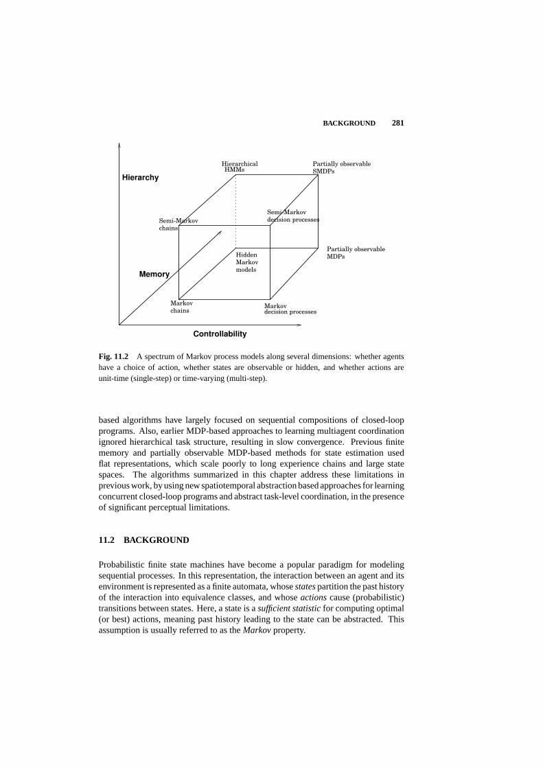
BACKGROUND 281
Markov
chains
Partially observable
MDPs
Semi-Markov
decision processes
Hidden
Markov
models
Partially observable
SMDPs
HierarchicalHMMs
Markovdecision processes
Controllability
Hierarchy
Semi-Markov
chains
Memory
Fig. 11.2 A spectrum of Markov process models along several dimensions: whether agentshave a choice of action, whether states are observable or hidden, and whether actions areunit-time (single-step) or time-varying (multi-step).
based algorithms have largely focused on sequential compositions of closed-loopprograms. Also, earlier MDP-based approaches to learning multiagent coordinationignored hierarchical task structure, resulting in slow convergence. Previous finitememory and partially observable MDP-based methods for state estimation usedflat representations, which scale poorly to long experience chains and large statespaces. The algorithms summarized in this chapter address these limitations inprevious work, by using new spatiotemporal abstraction based approaches for learningconcurrent closed-loop programs and abstract task-level coordination, in the presenceof significant perceptual limitations.
11.2 BACKGROUND
Probabilistic finite state machines have become a popular paradigm for modelingsequential processes. In this representation, the interaction between an agent and itsenvironment is represented as a finite automata, whosestatespartition the past historyof the interaction into equivalence classes, and whoseactionscause (probabilistic)transitions between states. Here, a state is asufficient statisticfor computing optimal(or best) actions, meaning past history leading to the state can be abstracted. Thisassumption is usually referred to as theMarkovproperty.

282 CONCURRENCY, MULTIAGENCY, AND PARTIAL OBSERVABILITY
Markov processes have become the mathematical foundation for much current workin reinforcement learning [36], decision-theoretic planning [2], information retrieval[8], speech recognition [11], active vision [22], and robot navigation [14]. In thischapter, we are interested in abstracting sequential Markov processes using twostrategies: state aggregation/decomposition and temporal abstraction. State decom-position methods typically represent states as collections offactoredvariables [2],or simplify the automaton by eliminating “useless” states [4]. Temporal abstractionmechanisms, for example in hierarchical reinforcement learning [37, 6, 25], encap-sulate lower-level observation or action sequences into a single unit at more abstractlevels. For a unified algebraic treatment of abstraction of Markov decision processesthat covers both spatial and temporal abstraction, the reader is referred to [29].
Figure 11.2 illustrates eight Markov process models, arranged in a cube whose axesrepresent significant dimensions along which the models differ from each other.While a detailed description of each model is beyond the scope of this chapter, wewill provide brief descriptions of many of these models below, beginning in thissection with the basic MDP model.
A Markov decision process(MDP) [28] is specified by a set of statesS, a set ofallowable actionsA(s) in each states, and a transition function specifying the next-state distributionP a
ss′ for each actiona ∈ A(s). A reward or cost functionr(s, a)specifies theexpectedreward for carrying out actiona in states. Solving a givenMDP requires finding an optimal mapping orpolicy π∗ : S → A that maximizesthe long-term cumulative sum of rewards (usually discounted by some factorγ < 1)or the expected average-reward per step. A classic result is that for any MDP, thereexists a stationary deterministic optimal policy, which can be found by solving anonlinear set of equations, one for each state (such as by a successive approximationmethod calledvalue iteration):
V ∗(s) = maxa∈A(s)
(r(s, a) + γ
∑
s′P a
ss′V∗(s′)
)(11.1)
MDPs have been applied to many real-world domains, ranging from robotics [14, 17]to engineering optimization [3, 18], and game playing [39]. In many such domains,the model parameters (rewards, transition probabilities) are unknown, and need tobe estimated from samples generated by the agent exploring the environment. Q-learning was a major advance in direct policy learning, since it obviates the need formodel estimation [45]. Here, the Bellman optimality equation is reformulated usingaction valuesQ∗(x, a), which represent the value of the non-stationary policy ofdoing actiona once, and thereafter acting optimally. Q-learning eventually finds theoptimal policy asymptotically. However, much work is required in scaling Q-learningto large problems, and abstraction is one of the key components. Factored approachesto representing value functions may also be key to scaling to large problems [15].
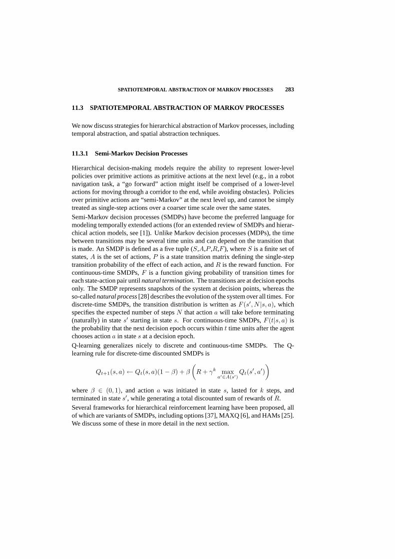
SPATIOTEMPORAL ABSTRACTION OF MARKOV PROCESSES 283
11.3 SPATIOTEMPORAL ABSTRACTION OF MARKOV PROCESSES
We now discuss strategies for hierarchical abstraction of Markov processes, includingtemporal abstraction, and spatial abstraction techniques.
11.3.1 Semi-Markov Decision Processes
Hierarchical decision-making models require the ability to represent lower-levelpolicies over primitive actions as primitive actions at the next level (e.g., in a robotnavigation task, a “go forward” action might itself be comprised of a lower-levelactions for moving through a corridor to the end, while avoiding obstacles). Policiesover primitive actions are “semi-Markov” at the next level up, and cannot be simplytreated as single-step actions over a coarser time scale over the same states.
Semi-Markov decision processes (SMDPs) have become the preferred language formodeling temporally extended actions (for an extended review of SMDPs and hierar-chical action models, see [1]). Unlike Markov decision processes (MDPs), the timebetween transitions may be several time units and can depend on the transition thatis made. An SMDP is defined as a five tuple (S,A,P ,R,F ), whereS is a finite set ofstates,A is the set of actions,P is a state transition matrix defining the single-steptransition probability of the effect of each action, andR is the reward function. Forcontinuous-time SMDPs,F is a function giving probability of transition times foreach state-action pair untilnatural termination. The transitions are at decision epochsonly. The SMDP represents snapshots of the system at decision points, whereas theso-callednatural process[28] describes the evolution of the system over all times. Fordiscrete-time SMDPs, the transition distribution is written asF (s′, N |s, a), whichspecifies the expected number of stepsN that actiona will take before terminating(naturally) in states′ starting in states. For continuous-time SMDPs,F (t|s, a) isthe probability that the next decision epoch occurs withint time units after the agentchooses actiona in states at a decision epoch.
Q-learning generalizes nicely to discrete and continuous-time SMDPs. The Q-learning rule for discrete-time discounted SMDPs is
Qt+1(s, a) ← Qt(s, a)(1− β) + β
(R + γk max
a′∈A(s′)Qt(s′, a′)
)
whereβ ∈ (0, 1), and actiona was initiated in states, lasted fork steps, andterminated in states′, while generating a total discounted sum of rewards ofR.
Several frameworks for hierarchical reinforcement learning have been proposed, allof which are variants of SMDPs, including options [37], MAXQ [6], and HAMs [25].We discuss some of these in more detail in the next section.

284 CONCURRENCY, MULTIAGENCY, AND PARTIAL OBSERVABILITY
0.5
0.5
1.0
0.70.3
0.9 0.1
1.0 0.3
0.70.50.3
0.2
0.40.2
0.6 0.8 1.0
s1
s2 s3
s4 s5
s6 s7 s8
e1
e3
e4
Fig. 11.3 An example hierarchical hidden Markov model. Only leaf nodes produce obser-vations. Internal nodes can be viewed as generating sequences of observations.
11.3.2 Hierarchical Hidden Markov Models
Hidden Markov models (HMMs) are a widely-used probabilistic model for represent-ing time-series data, such as speech [11]. Unlike an MDP, states are not perceivable,and instead the agent receives an observationo which can be viewed as being gener-ated by a stochastic processP (o|s) as a function of the underlying states. HMMshave been widely applied to many time-series problems, ranging from speech recog-nition [11], information extraction [8], and bioinformatics [12]. However, like MDPs,HMMs do not provide any direct way of representing higher-level structure that isoften present in many practical problems. For example, an HMM can be used as aspatial representation of indoor environments [34], but typically such environmentshave higher order structures such as corridors or floors which are not made explicit inthe underlying HMM model. As in the case with MDPs, in most practical problems,the parameters of the underlying HMM have to be learned from samples. The mostpopular method for learning an HMM model is the Baum-Welch procedure, which isitself a special case of the more general Expectation-Maximization (EM) statisticalinference algorithm.
Recently, an elegant hierarchical extension of HMMs was proposed [7]. The HHMMgeneralizes the standard hidden Markov model by allowing hidden states to representstochastic processes themselves. An HHMM is visualized as a tree structure (see Fig-ure 11.3) in which there are three types of states, production states (leaves of the tree)which emit observations, and internal states which are (unobservable) hidden states
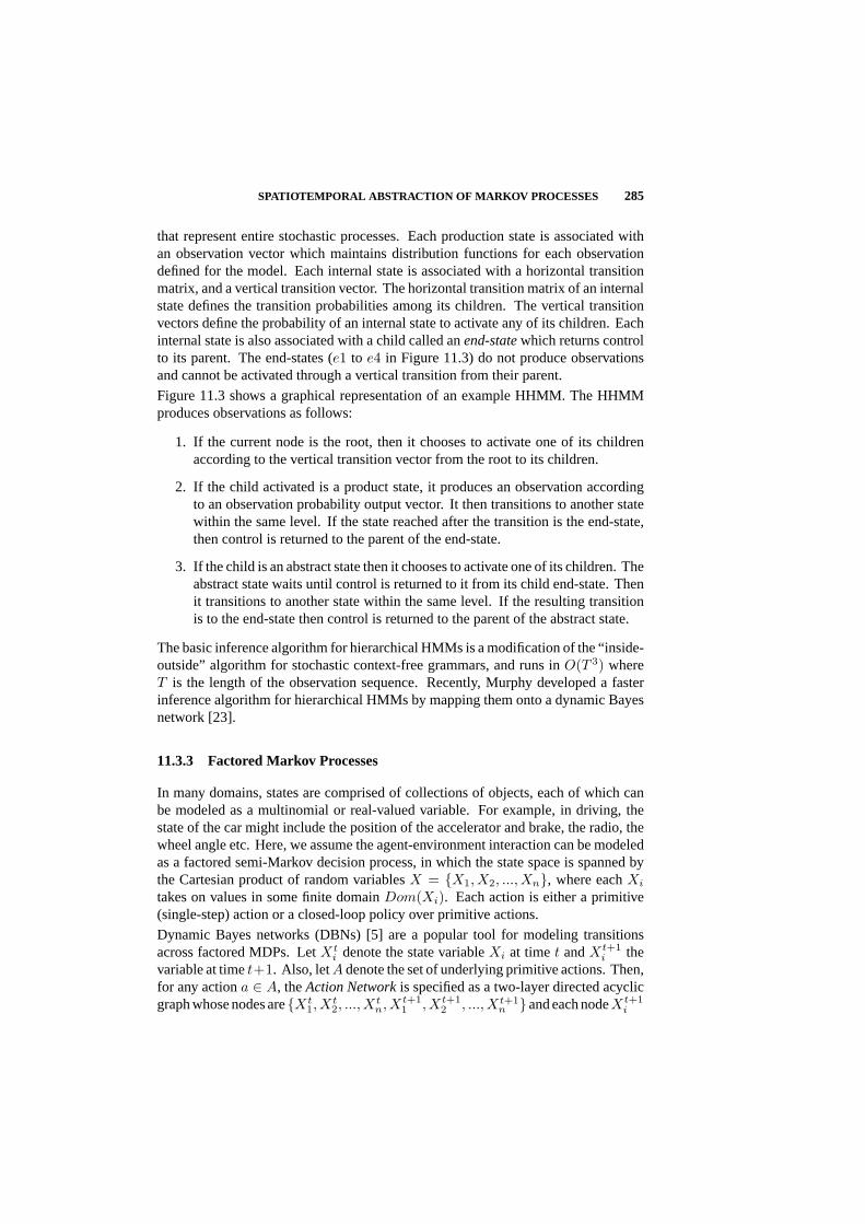
SPATIOTEMPORAL ABSTRACTION OF MARKOV PROCESSES 285
that represent entire stochastic processes. Each production state is associated withan observation vector which maintains distribution functions for each observationdefined for the model. Each internal state is associated with a horizontal transitionmatrix, and a vertical transition vector. The horizontal transition matrix of an internalstate defines the transition probabilities among its children. The vertical transitionvectors define the probability of an internal state to activate any of its children. Eachinternal state is also associated with a child called anend-statewhich returns controlto its parent. The end-states (e1 to e4 in Figure 11.3) do not produce observationsand cannot be activated through a vertical transition from their parent.
Figure 11.3 shows a graphical representation of an example HHMM. The HHMMproduces observations as follows:
1. If the current node is the root, then it chooses to activate one of its childrenaccording to the vertical transition vector from the root to its children.
2. If the child activated is a product state, it produces an observation accordingto an observation probability output vector. It then transitions to another statewithin the same level. If the state reached after the transition is the end-state,then control is returned to the parent of the end-state.
3. If the child is an abstract state then it chooses to activate one of its children. Theabstract state waits until control is returned to it from its child end-state. Thenit transitions to another state within the same level. If the resulting transitionis to the end-state then control is returned to the parent of the abstract state.
The basic inference algorithm for hierarchical HMMs is a modification of the “inside-outside” algorithm for stochastic context-free grammars, and runs inO(T 3) whereT is the length of the observation sequence. Recently, Murphy developed a fasterinference algorithm for hierarchical HMMs by mapping them onto a dynamic Bayesnetwork [23].
11.3.3 Factored Markov Processes
In many domains, states are comprised of collections of objects, each of which canbe modeled as a multinomial or real-valued variable. For example, in driving, thestate of the car might include the position of the accelerator and brake, the radio, thewheel angle etc. Here, we assume the agent-environment interaction can be modeledas a factored semi-Markov decision process, in which the state space is spanned bythe Cartesian product of random variablesX = X1, X2, ..., Xn, where eachXi
takes on values in some finite domainDom(Xi). Each action is either a primitive(single-step) action or a closed-loop policy over primitive actions.
Dynamic Bayes networks (DBNs) [5] are a popular tool for modeling transitionsacross factored MDPs. LetXt
i denote the state variableXi at timet andXt+1i the
variable at timet+1. Also, letA denote the set of underlying primitive actions. Then,for any actiona ∈ A, theAction Networkis specified as a two-layer directed acyclicgraph whose nodes areXt
1, Xt2, ..., X
tn, Xt+1
1 , Xt+12 , ..., Xt+1
n and each nodeXt+1i
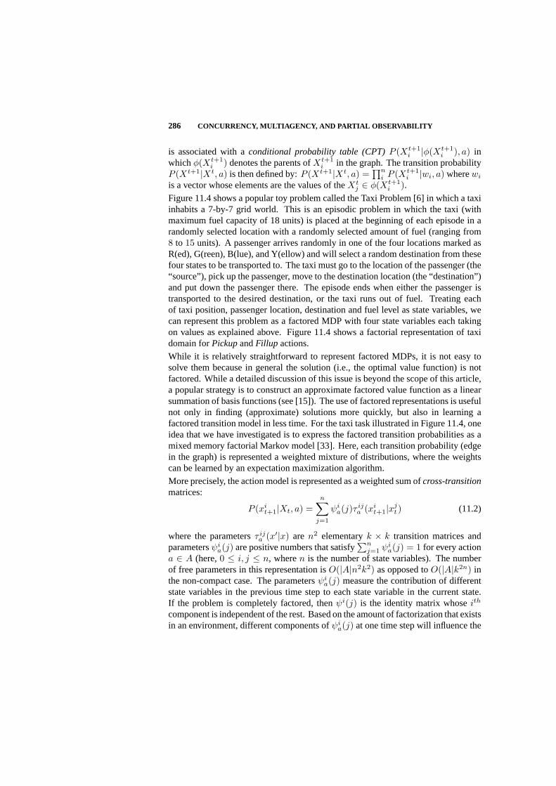
286 CONCURRENCY, MULTIAGENCY, AND PARTIAL OBSERVABILITY
is associated with aconditional probability table (CPT)P (Xt+1i |φ(Xt+1
i ), a) inwhichφ(Xt+1
i ) denotes the parents ofXt+1i in the graph. The transition probability
P (Xt+1|Xt, a) is then defined by:P (Xt+1|Xt, a) =∏n
i P (Xt+1i |wi, a) wherewi
is a vector whose elements are the values of theXtj ∈ φ(Xt+1
i ).Figure 11.4 shows a popular toy problem called the Taxi Problem [6] in which a taxiinhabits a 7-by-7 grid world. This is an episodic problem in which the taxi (withmaximum fuel capacity of 18 units) is placed at the beginning of each episode in arandomly selected location with a randomly selected amount of fuel (ranging from8 to 15 units). A passenger arrives randomly in one of the four locations marked asR(ed), G(reen), B(lue), and Y(ellow) and will select a random destination from thesefour states to be transported to. The taxi must go to the location of the passenger (the“source”), pick up the passenger, move to the destination location (the “destination”)and put down the passenger there. The episode ends when either the passenger istransported to the desired destination, or the taxi runs out of fuel. Treating eachof taxi position, passenger location, destination and fuel level as state variables, wecan represent this problem as a factored MDP with four state variables each takingon values as explained above. Figure 11.4 shows a factorial representation of taxidomain forPickupandFillup actions.
While it is relatively straightforward to represent factored MDPs, it is not easy tosolve them because in general the solution (i.e., the optimal value function) is notfactored. While a detailed discussion of this issue is beyond the scope of this article,a popular strategy is to construct an approximate factored value function as a linearsummation of basis functions (see [15]). The use of factored representations is usefulnot only in finding (approximate) solutions more quickly, but also in learning afactored transition model in less time. For the taxi task illustrated in Figure 11.4, oneidea that we have investigated is to express the factored transition probabilities as amixed memory factorial Markov model [33]. Here, each transition probability (edgein the graph) is represented a weighted mixture of distributions, where the weightscan be learned by an expectation maximization algorithm.
More precisely, the action model is represented as a weighted sum ofcross-transitionmatrices:
P (xit+1|Xt, a) =
n∑
j=1
ψia(j)τ ij
a (xit+1|xj
t ) (11.2)
where the parametersτ ija (x′|x) are n2 elementaryk × k transition matrices and
parametersψia(j) are positive numbers that satisfy
∑nj=1 ψi
a(j) = 1 for every actiona ∈ A (here,0 ≤ i, j ≤ n, wheren is the number of state variables). The numberof free parameters in this representation isO(|A|n2k2) as opposed toO(|A|k2n) inthe non-compact case. The parametersψi
a(j) measure the contribution of differentstate variables in the previous time step to each state variable in the current state.If the problem is completely factored, thenψi(j) is the identity matrix whoseith
component is independent of the rest. Based on the amount of factorization that existsin an environment, different components ofψi
a(j) at one time step will influence the
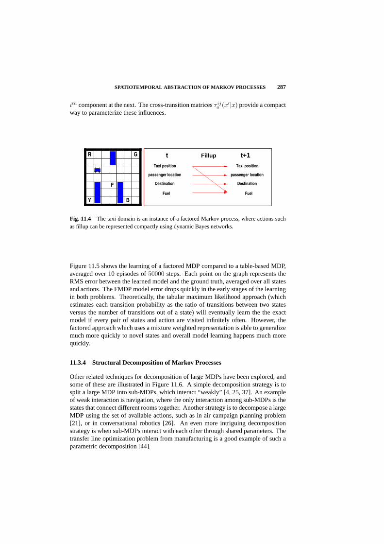
SPATIOTEMPORAL ABSTRACTION OF MARKOV PROCESSES 287
ith component at the next. The cross-transition matricesτ ija (x′|x) provide a compact
way to parameterize these influences.
R G
BY
F
t
passenger location
Taxi position
Destination
Fuel
passenger location
t+1
Taxi position
Destination
Fuel
Fillup
Fig. 11.4 The taxi domain is an instance of a factored Markov process, where actions suchas fillup can be represented compactly using dynamic Bayes networks.
Figure 11.5 shows the learning of a factored MDP compared to a table-based MDP,averaged over 10 episodes of50000 steps. Each point on the graph represents theRMS error between the learned model and the ground truth, averaged over all statesand actions. The FMDP model error drops quickly in the early stages of the learningin both problems. Theoretically, the tabular maximum likelihood approach (whichestimates each transition probability as the ratio of transitions between two statesversus the number of transitions out of a state) will eventually learn the the exactmodel if every pair of states and action are visited infinitely often. However, thefactored approach which uses a mixture weighted representation is able to generalizemuch more quickly to novel states and overall model learning happens much morequickly.
11.3.4 Structural Decomposition of Markov Processes
Other related techniques for decomposition of large MDPs have been explored, andsome of these are illustrated in Figure 11.6. A simple decomposition strategy is tosplit a large MDP into sub-MDPs, which interact “weakly” [4, 25, 37]. An exampleof weak interaction is navigation, where the only interaction among sub-MDPs is thestates that connect different rooms together. Another strategy is to decompose a largeMDP using the set of available actions, such as in air campaign planning problem[21], or in conversational robotics [26]. An even more intriguing decompositionstrategy is when sub-MDPs interact with each other through shared parameters. Thetransfer line optimization problem from manufacturing is a good example of such aparametric decomposition [44].

288 CONCURRENCY, MULTIAGENCY, AND PARTIAL OBSERVABILITY
0
0.02
0.04
0.06
0.08
0.1
0.12
0.14
0.16
0 10000 20000 30000 40000 50000
RM
S E
rro
r
Steps
Taxi domain
Tabular Maximum-LikelihoodFMDP
Fig. 11.5 Comparing factored versus tabular model learning performance in the taxi domain.
Room 3
Room 1
Room 4
x x
xx x
x
x x
$
Room 2 x
x
x x
x x
$
a) b)
Task 2 Task n
Available Action Set
Task 1
MTS
Fig. 11.6 State and action-based decomposition of Markov processes.
11.4 CONCURRENCY, MULTIAGENCY, AND PARTIALOBSERVABILITY
This section summarizes our recent research on exploiting spatiotemporal abstractionto produce improved solutions to three difficult problems in sequential decision-making: learning plans involving concurrent action, multiagent coordination, andusing memory to estimate hidden state.
11.4.1 A Hierarchical Framework for Concurrent Action
We now describe a probabilistic model for learning concurrent plans over temporallyextended actions [30, 31]. The notion of concurrent action is formalized in a generalway, to capture both situations where a single agent can execute multiple parallel

CONCURRENCY, MULTIAGENCY, AND PARTIAL OBSERVABILITY 289
processes, as well as the multi-agent case where many agents act in parallel.
The Concurrent Action Model (CAM)is defined as(S,A, T ,R), whereS is a setof states,A is a set ofprimary actions,T is a transition probability distributionS ×wp(A)×S ×N → [0, 1], where wp(A) is the power-set of the primary actionsandN is the set of natural numbers, andR is the reward function mappingS → <.Here, a concurrent action is simply represented as a set of primary actions (hereaftercalled amulti-action), where each primary action is either a single step action, or atemporally extended action(e.g., modeled as a closed loop policy over single stepactions [37]).
Figure 11.7 illustrates a toy example of concurrent planning. The general problem isas follows. The agent is given a set of primary actions, each of which can be viewedas a (fixed or previously learned) “subroutine” for choosing actions over a subspaceof the overall state space. The goal of the agent is to learn to construct a closed-loopplan (or policy) that allows multiple concurrent subroutines to be executed in parallel(and in sequence) to achieve the task at hand. For multiple primary actions to beexecuted concurrently, their joint semantics must be well-defined. Concurrency isfacilitated by assuming states are not atomic, but structured as a collection of (discreteor continuous) variables, and the effect of actions on such sets of variables can becaptured by a compact representation, such as a dynamic Bayes net (DBN) [5].
(to each room’s 2 hallways)- One single step no-op option
- 8 multi-step navigation options
- 3 stochastic primitive actions for keys(get-key, key-nop and putback-key)
each key- Drops the keys 20% of times when passingthrough the water trap and holding both keys
- 2 multi-step key options (pickup-key) for
water trap
and holding both keys
- 4 stochastic primitive actions(Up, Down, Left and Right)- Fail 10% of times, when not passingthe water trap- Fail 30% of times, when passing thewater trap
Agent H0
H2
H1 H3 (Goal)
Fig. 11.7 A grid world problem to illustrate concurrent planning: the agent is given subrou-tines for getting to each door from any interior room state, and for opening a locked door. Ithas to learn the shortest path to the goal by concurrently combining these subroutines. Theagent can reach the goal more quickly if it learns to parallelize the subroutine for retrieving thekey before it reaches a locked door. However, retrieving the key too early is counterproductivesince it can drop with some probability.

290 CONCURRENCY, MULTIAGENCY, AND PARTIAL OBSERVABILITY
Since multiple concurrent primary actions may not terminate synchronously, thenotion of a decision epoch needs to be generalized. For example, a decision epochcan occur when any one of the actions currently running terminates. We refer tothis as theTany termination condition (Figure 11.8, left). Alternatively, a decisionepoch can be defined to occur when all actions currently running terminate, which werefer to as theTall condition (Figure 11.8, middle). We can design other terminationschemes by combiningTany and Tall : for example, another termination schemecalledcontinueis one that always terminates based on theTany termination scheme,but lets those primary actions that did not terminate naturally continue running, whileinitiating new primary actions if they are going to be useful (Figure 11.8, right).
ts
t t+k
nd 1+nd
1o2o
4o3o
interrupted,,, 4321 oooo=multi-option
ts
t
nd 1+nd
1o2o
4o3o
,,, 4321 oooo=multi-option
no-op
ts
t t+k
nd 1+nd
1o2o
4o3o
Continue to run,,, 4321 oooo=
Current multi-option
1'o
,,,' 4321 oooo=N ext multi-option
Fig. 11.8 Left: Tanytermination scheme. Middle:Tall termination scheme. Right:Tcontinue termination scheme.
For concreteness, we will describe the concurrent planning framework when theprimary actions are represented asoptions [37]. The treatment here is restrictedto options over discrete-time SMDPs and deterministic policies, but the main ideasextend readily to other hierarchical formalisms [6, 25] and to continuous-time SMDPs[9, 28]. More formally, an optiono consists of three components: a policyπ : S → A,a termination conditionβ : S → [0, 1], and an initiation setI ⊆ S, whereI denotesthe set of statess in which the option can be initiated. For any states, if option π istaken, then primitive actions are selected based onπ until it terminates according toβ. An optiono is aMarkov optionif its policy, initiation set and termination conditiondepend stochastically only on the current states ∈ S. An optiono is semi-Markovifits policy, initiation set and termination condition are dependent on all prior historysince the option was initiated. For example, the optionexit-roomin the grid worldenvironment shown in Figure 11.7, in which states are the different locations in theroom, is a Markov option, since for a given location, the direction to move to get tothe door can be computed given the current state.
A hierarchical policy over primary actions or options can be defined as follows. TheMarkov policy over optionsµ : S → O (whereO is the set of all options) selectsan optiono ∈ O at timet using the functionµ(st). The optiono is then initiated inst until it terminates at a random timet + k in some statest+k according to a giventermination condition, and the process repeats inst+k.
The multistep state transition dynamics over options is defined using the discountfactor to weight the probability of transitioning. Letpo(s, s′, k) denote the probabilitythat the optiono is initiated in states and terminates in states′ afterk steps. Thenp(s′|s, o) =
∑∞k=1 po(s, s′, k)γk (note that whenγ < 1, the transition model is not

CONCURRENCY, MULTIAGENCY, AND PARTIAL OBSERVABILITY 291
a stochastic matrix, since the distributions do not sum to 1). If multi-step models ofoptions and rewards are known, optimal hierarchical plans can be found by solving ageneralized Bellman equation over options similar to Eq. 11.1. Under either definitionof the termination event (i.e.;Tany , Tall , andTcontinue ), the following result holds.
Theorem 11.4.1Given a Markov decision process, and a set of concurrent Markovoptions defined on it, the decision process that selects only among multi-actions, andexecutes each one until its termination according to a given termination conditionforms a semi-Markov decision process.
The proof requires showing that the state transition dynamicsp(s′, N |~a, s) and therewardsr(s,~a) over any concurrent action~a defines a semi-Markov decision process[30]. The significance of this result is that SMDP Q-learning methods can be extendedto learn concurrent plans under this model. The extended SMDP Q-learning algorithmfor learning to plan with concurrent actions updates the multi-action-value functionQ(s,~a) after each decision epoch where the multi-action~a is taken in some statesand terminates ins′ (under a specific termination condition):
Q(s,~a) ← Q(s,~a)(1− β) + β
[R + γk max
~a′∈Os′Q(s′, ~a′)
](11.3)
wherek denotes the number of time steps between initiation of the multi-action~oin states and its termination in states′, andR denotes the cumulative discountedreward over this period. The result of using this algorithm on the simple grid worldproblem in shown in Figure 11.9. The figure illustrates the difference in performanceunder different termination conditions (Tall, Tany, andTcontinue).
The performance of the concurrent action model also depends on the termination eventdefined for that model. Each termination event trades-off between the optimality ofthe learned plan and how fast it converges to its optimal policy. Letπ∗seq , π∗all andπ∗any denote the optimal policy when the primary actions are executed sequentially;when termination constructTall is used; and when termination constructTany isused, respectively. Also letπcontinue represent the policy learned based on theTcontinue termination construct. Intuitively, the models with a termination constructthat imposes more frequent multi-action termination (such asTany andTcontinue ),tend toarticulate more frequently and should perform more optimally. Howeverdue to more interruption, they may converge more slowly to their optimal behavior.Based on the definition of each termination construct we can prove the followingtheorem:
Theorem 11.4.2 In a concurrent action model and a set of termination schemesTany, Tall, continue, the following partial ordering holds among the optimal pol-icy based onTany , the optimal policy based onTall , the continuepolicy and theoptimal sequential policy:π∗seq ≤ π∗all ≤ πcontinue ≤ π∗any .
where≤ denotes the partial ordering relation over policies.

292 CONCURRENCY, MULTIAGENCY, AND PARTIAL OBSERVABILITY
20
25
30
35
40
45
50
55
60
65
70
0 100000 200000 300000 400000 500000
Med
ian/
Tria
ls (
step
s to
goa
l)
Trial
Sequential ActionsConcurrent Actions: T-all
Concurrent Actions: T-anyConcurrent Actions: T-continue
Fig. 11.9 This graph compares an SMDP technique for learning concurrent plans (undervarious termination conditions) with a slower “get-to-door-then-pickup-key” sequential planlearner. The concurrent learners outperform the sequential learner, but the choice of terminationaffects the speed and quality of the final plan.
Tall
Tany
Continue multi-action policies
Multi-action policies using
Multi-action policies using
Policies over sequential actions
Fig. 11.10 Comparison of policies over multi-actions and sequential primary actions usingdifferent termination schemes.
Figure 11.10 illustrates the results defined by Theorem 11.4.2. According to thisfigure, the optimal multi-action policies based onTany andTall , and alsocontinuemulti-action policies dominate (with respect to the partial ordering relation definedover policies) the optimal policies over the sequential case. Furthermore, policiesbased oncontinuemulti-actions dominate the optimal multi-action policies based onTall termination scheme, while themselves being dominated by the optimal multi-action policies based onTany termination scheme.
11.4.2 Learning Multiagent Task-Level Coordination Strategies
The second case study uses hierarchical abstraction to design efficient learning algo-rithms forcooperativemultiagent systems [46]. Figure 11.11 illustrates a multiagentautomated guided vehicle (AGV) scheduling task, where four AGV agents will max-imize their performance at the task if they learn to coordinate with each other. The
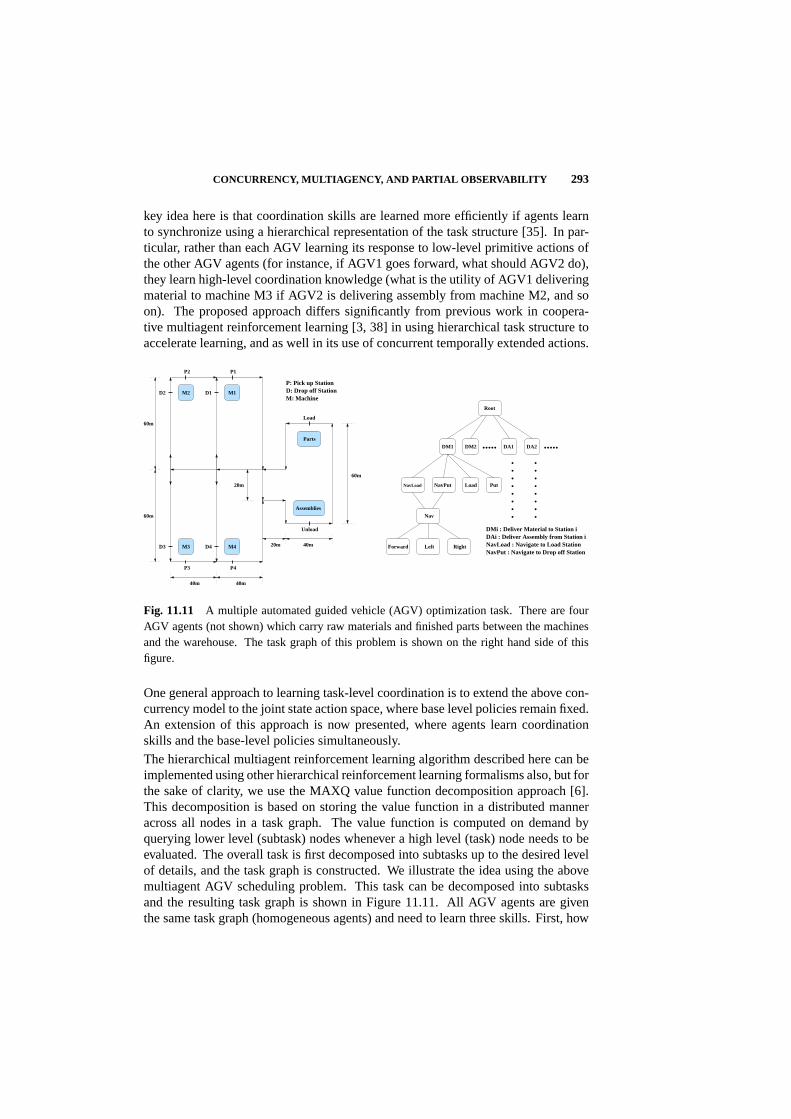
CONCURRENCY, MULTIAGENCY, AND PARTIAL OBSERVABILITY 293
key idea here is that coordination skills are learned more efficiently if agents learnto synchronize using a hierarchical representation of the task structure [35]. In par-ticular, rather than each AGV learning its response to low-level primitive actions ofthe other AGV agents (for instance, if AGV1 goes forward, what should AGV2 do),they learn high-level coordination knowledge (what is the utility of AGV1 deliveringmaterial to machine M3 if AGV2 is delivering assembly from machine M2, and soon). The proposed approach differs significantly from previous work in coopera-tive multiagent reinforcement learning [3, 38] in using hierarchical task structure toaccelerate learning, and as well in its use of concurrent temporally extended actions.
P: Pick up StationD: Drop off StationM: Machine
Forward Left Right
Nav
NavLoad NavPut PutLoad
DM1 DM2 DA2DA1
Root
.
.
.
.
.
.
.
.
.
.
.
.
.DMi : Deliver Material to Station iDAi : Deliver Assembly from Station iNavLoad : Navigate to Load StationNavPut : Navigate to Drop off Station
D2
D4D3
D1
P1P2
P3 P4
Unload
Load
20m
60m
40m20m
60m
40m 40m
60m
M3
M2
M4
M1
Parts
Assemblies
..... .....
.
.
.
Fig. 11.11 A multiple automated guided vehicle (AGV) optimization task. There are fourAGV agents (not shown) which carry raw materials and finished parts between the machinesand the warehouse. The task graph of this problem is shown on the right hand side of thisfigure.
One general approach to learning task-level coordination is to extend the above con-currency model to the joint state action space, where base level policies remain fixed.An extension of this approach is now presented, where agents learn coordinationskills and the base-level policies simultaneously.
The hierarchical multiagent reinforcement learning algorithm described here can beimplemented using other hierarchical reinforcement learning formalisms also, but forthe sake of clarity, we use the MAXQ value function decomposition approach [6].This decomposition is based on storing the value function in a distributed manneracross all nodes in a task graph. The value function is computed on demand byquerying lower level (subtask) nodes whenever a high level (task) node needs to beevaluated. The overall task is first decomposed into subtasks up to the desired levelof details, and the task graph is constructed. We illustrate the idea using the abovemultiagent AGV scheduling problem. This task can be decomposed into subtasksand the resulting task graph is shown in Figure 11.11. All AGV agents are giventhe same task graph (homogeneous agents) and need to learn three skills. First, how

294 CONCURRENCY, MULTIAGENCY, AND PARTIAL OBSERVABILITY
to do each subtask, such as deliver parts to machine M1 or navigation to drop offstation D3, and when to perform load or put action. Second, the agents also needto learn the order to do subtasks (for instance go to pick up station of a machineand pick up an assembly, before heading to the unload station). Finally, the agentsalso need to learn how to coordinate with other agents (i.e. AGV1 can deliver partsto machine M4 whereas AGV3 can deliver assemblies from machine M2). We candistinguish between two learning approaches. In theselfishcase, the agents learnwith the given task graph, but make no attempt to coordinate with each other. Inthe cooperativecase, coordination skills among agents are learned by using jointactions at the level(s) immediately under the root task. Therefore, it is necessary togeneralize the MAXQ decomposition from its original sequential single-agent settingto the concurrent multiagent coordination problem. We call this extension of MAXQ,cooperativeMAXQ [19]. In this algorithm, each agent learns joint abstract actionvalues by communicating with other agents only the high-level subtasks that they aredoing. Since high-level tasks can take a long time to complete, communication isneeded only fairly infrequently, which is a significant advantage over flat methods.A further advantage is that agents learn coordination skills at the level of abstractactions and it allows for increased cooperation skills as agents do not get confusedby low level details. In addition, each agent has only local state information and isignorant about the other agent’s state. Keeping track of just local information greatlysimplifies the underlying reinforcement learning problem. This is based on the ideathat in many cases, the state of the other agent might be roughly estimated just byknowing about the high-level action being performed by the other agent.
Let ~s = (s1, . . . , sn) and~a = (a1, . . . , an) denote a joint state and a concurrentaction, wheresi is the local state andai is the action being performed by agenti. Letthe joint action value functionQ(p,~s,~a) represents the value of concurrent action~ain joint state~s, in the context of executing parent taskp.
The MAXQ decomposition of the Q-function relies on a key principle: the rewardfunction for the parent task is essentially the value function of the child subtask. Thisprinciple can be extended to joint concurrent action values as shown below. Themost salient feature of thecooperativeMAXQ algorithm, is that the top level(s) (thelevel immediately below the root and perhaps lower levels) of the hierarchy is (are)configured to store thecompletion functionvalues for joint abstract actions of allagents. Thecompletion functionC(p,~s,~a) is the expected cumulative discountedreward of completing parent taskp after finishing concurrent action~a, which wasinvoked in state~s. The joint concurrent value functionV (p,~s) is now approximatedby each agenti (given only its local statesi) as:
V i(p, si) =
maxai Qi(p, si,~a) if p is a composite action∑s′i
P (s′i|si, p)R(s′j |sj , p) if p is a primitive action
where the action value function of agenti (given only its local statesi) is defined as
Qi(p, si,~a) ≈ V i(ai, si) + Ci(p, si,~a) (11.4)

CONCURRENCY, MULTIAGENCY, AND PARTIAL OBSERVABILITY 295
The first term in Eq. 11.4,V i(ai, si), refers to the discounted sum of rewards receivedby agenti for performing actionai in local statesi. The second term,Ci(p, si,~a),completes the sum by accounting for rewards earned for completing the parent taskp after finishing subtaskai. The completion function is updated in this algorithmfrom sample values using an SMDP learning rule. Note that the correct action valueis approximated by only considering local statesi and also by ignoring the effect ofconcurrent actionsak, k 6= i by other agents when agenti is performing actionai.In practice, a human designer can configure the task graph to store joint concurrentaction-values at the highest (or lower than the highest as needed) level(s) of thehierarchy.
To illustrate the use of this decomposition in learning multiagent coordination for theAGV scheduling task, if the joint action-values are restricted to only the highest levelof the task graph under the root, we get the following value function decompositionfor AGV1:
Q1(Root, s1, DM3, DA2, DA4, DM1) ≈ V
1(DM3, s1) + C
1(Root, s1, DM3, DA2, DA4, DM1)
which represents the value of AGV1 performing task DM3 in the context of theoverall root task, when AGV2, AGV3 and AGV4 are executing DA2, DA4 and DM1.Note that this value is decomposed into the value of AGV1 performing DM3 subtaskitself and the completion sum of the remainder of the overall task done by all fouragents.
Figure 11.12 compares the performance and speed of thecooperativeMAXQ al-gorithm with other learning algorithms, including single-agent MAXQ and selfishmultiagent MAXQ, as well as several well-known AGV scheduling heuristics like“first come first serve”, “highest queue first” and “nearest station first”.
0
2
4
6
8
10
12
14
0 5000 10000 15000 20000 25000 30000 35000 40000
Thr
ough
put o
f the
sys
tem
Time since start of simulation (sec)
Co-operating Multi-Agent MAXQSelfish Multi-Agent MAXQ
Single Agent MAXQ
0
2
4
6
8
10
12
14
0 5000 10000 15000 20000 25000 30000 35000 40000
Thr
ough
put o
f the
sys
tem
Time since start of simulation (sec)
Co-operative Multi-Agent MAXQFirst Come First Served Heuristic
Highest Queue First HeuristicNearest Station First Heuristic
Fig. 11.12 This figure compares the performance of thecooperativeMAXQ algorithm withother learning methods, including single-agent MAXQ and selfish multiagent MAXQ, as wellas several well-known AGV scheduling heuristics. The throughput is measured in terms of thenumber of finished assemblies deposited at the unload station per unit time.

296 CONCURRENCY, MULTIAGENCY, AND PARTIAL OBSERVABILITY
11.4.3 Hierarchical Memory
When agents learn to act concurrently in real-world environments, the true state of theenvironment is usually hidden. To address this issue, we need to combine the abovemethods for learning concurrency and coordination with methods for estimatinghidden state. We have explored two multiscale memory models [10, 42].HierarchicalSuffix Memory(HSM) [10] generalizes the suffix tree model [20] to SMDP-basedtemporally extended actions. Suffix memory constructs state estimators from finitechains of observation-action-reward triples. In addition to extending suffix modelsto SMDP actions, HSM also uses multiple layers of temporal abstraction to formlonger-term memories at more abstract levels. Figure 11.13 illustrates this idea forrobot navigation for the simpler case of a linear chain, although the tree-based modelhas also been investigated. An important side-effect is that the agent can look backmany steps back in time while ignoring the exact sequence of low-level observationsand actions that transpired. Tests in a robot navigation domain showed that HSMoutperformed “flat” suffix tree methods, as well as hierarchical methods that used nomemory [10].
. . .. . . . . .
*?
T-junctioncorner dead end
D3 D1 D3 D2 D1 D3
*. . . ?
d3 d2 d3d3 d2d2
abstraction level: navigation
abstraction level: traversal
abstraction level: primitive
Fig. 11.13 A hierarchical suffix memory state estimator for a robot navigation task. Atthe abstract (navigation) level, observations and decisions occur at intersections. At thelower (corridor-traversal) level, observations and decisions occur within the corridor. At eachlevel, each agent constructs states out of its past experience with similar history (shown withshadows).
Partially observable MDPs are theoretically more powerful than finite memory mod-els, but past work on POMDPs has mostly studied “flat” models for which learningand planning algorithms scale poorly with model size. We have developed a newhierarchical POMDPframework termed H-POMDPs (see Figure 11.14) [42], byextending the hierarchical hidden Markov model (HHMM) [7] to include rewards,multiple entry/exit points into abstract states and (temporally extended) actions.
H-POMDPs can also be represented as Dynamic Bayesian networks [43], in a similarway that HHMMs can be represented as DBNs [23]. Figure 11.15 shows a DynamicBayesian net representation of H-POMDPs. This model differs from the model

CONCURRENCY, MULTIAGENCY, AND PARTIAL OBSERVABILITY 297
Fig. 11.14 State transition diagram of a hierarchical POMDP used to model corridor envi-ronments. Large ovals represent abstract states; the small solid circles within them represententry states, and the small hollow circles represent exit states. The small circles with arrowsrepresent production states. Arcs represent non-zero transition probabilities as follows: Dottedarrows from concrete states represent concrete horizontal transitions, dashed arrows from exitstates represent abstract horizontal transitions, and solid arrows from entry states representvertical transitions.
described in [23] in two basic ways: the presence of action nodesA, and the fact thatexit nodesX are no longer binary.
O 1 O 2
11
21
22
12
1 2
1A A2
S
S
X
S
S
X
Fig. 11.15 A 2-level HPOMDP represented as a DBN.
In the particular navigation example shown in Figure 11.14, the exit nodeXt cantake on five possible values, representing no-exit, north-exit, east-exit, south-exit, andwest-exit. IfXt = no-exit, then we make a horizontal transition at the concrete level,but the abstract state is required to remain the same. IfXt 6= no-exit, then we entera new abstract state; this abstract state then makes a vertical transition into a newconcrete state. The new concrete state,S1
t , depends on the new abstract state,S2t , as
298 CONCURRENCY, MULTIAGENCY, AND PARTIAL OBSERVABILITY
well as the previous exit state,Xt−1. More precisely we can define the conditionalprobability distributions of each type of node in the DBN as follows: For the abstractnodes,
P (S2t = s′|S2
t−1 = s,Xt−1 = x,At−1 = a) =
δ(s′, s) if x =no-exitT root(s′x|sx, a) otherwise
whereT root(s′x|sx, a) in the state representation of the HPOMDP model defines thetransition probability from abstract states and exit statex to abstract states′ andentry statex, wherex defines the type of entry or exit state (north, east, west, south).S is the parent ofs ands′ in the state transition model.
For the concrete nodes,
P (S1t = s′|S1
t−1 = s, S2t = S, Xt−1 = x,At−1 = a) =
TS(s′|s, a) if x =no-exitV (s′|Sx) otherwise
whereV (s′|Sx) defines the probability of a vertical transition from abstract stateSand entry state of typex to concrete states′.For the exit nodes,
P (Xt = x|S1t = s, S2
t = S, At = a) = TS(Sx|s, a)
whereTS(Sx|s, a) is the transition probability from production states under abstractstateS to exit from stateS of typex.
For the sensor nodes,
P (Ot = z|S1t = s, S2
t = S, At−1 = a) = OS(z|s, a)
whereOS(z|s, a) is the probability of perceiving observationz at thesth node understateS after actiona.
One of the most important differences of Hierarchical HMMs/POMDPs and flatmodels are the results of inference. In a hierarchical model a transition to an abstractstate at timet is zero, unless the abstract state is able to produce part of the remainingobservations and actions in a given sequence. The inference algorithm for the staterepresentation of HHMMs/H-POMDPs in [7], [42] achieves this by doing inferenceon all possible subsequences of observations under the different abstract states, whichleads toO(KDT 3) time, whereK is the number of states at each level of the hierarchyandD is the depth of the hierarchy. In a DBN representation we can achieve thesame result as the cubic time algorithms by asserting that the sequence has finished.In our particular implementation we assert that at the last time slice the sequencehas finished, and that there is a uniform probability of exit from any of the fourorientations. Since we have a DBN representation, we can apply any standard Bayesnet inference algorithm, such as junction tree, to perform filtering or smoothing whichtake in the worse caseO(K2DT ) time. Empirically it might be less, depending onthe size of the cliques being formed, as was shown in [23].
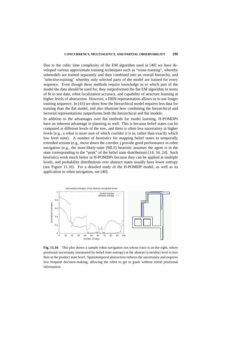
CONCURRENCY, MULTIAGENCY, AND PARTIAL OBSERVABILITY 299
Due to the cubic time complexity of the EM algorithm used in [40] we have de-veloped various approximate training techniques such as “reuse-training”, wherebysubmodels are trained separately and then combined into an overall hierarchy, and"selective-training" whereby only selected parts of the model are trained for everysequence. Even though these methods require knowledge as to which part of themodel the data should be used for, they outperformed the flat EM algorithm in termsof fit to test data, robot localization accuracy, and capability of structure learning athigher levels of abstraction. However, a DBN-representation allows us to use longertraining sequence. In [43] we show how the hierarchical model requires less data fortraining than the flat model, and also illustrate how combining the hierarchical andfactorial representations outperforms both the hierarchical and flat models.
In addition to the advantages over flat methods for model learning, H-POMDPshave an inherent advantage in planning as well. This is because belief states can becomputed at different levels of the tree, and there is often less uncertainty at higherlevels (e.g., a robot is more sure of which corridor it is in, rather than exactly whichlow level state). A number of heuristics for mapping belief states to temporallyextended actions (e.g., move down the corridor ) provide good performance in robotnavigation (e.g., the most-likely-state (MLS) heuristic assumes the agent is in thestate corresponding to the “peak” of the belief state distribution) [14, 34, 24]. Suchheuristics work much better in H-POMDPs because they can be applied at multiplelevels, and probability distributions over abstract states usually have lower entropy(see Figure 11.16). For a detailed study of the H-POMDP model, as well as itsapplication to robot navigation, see [40].
0
0.2
0.4
0.6
0.8
1
0 10 20 30 40 50 60 70 80 90 100
Nor
mal
ized
ent
ropi
es
Number of steps
Normalized entropies of the abstract and global levels
Global entropyAbstract entropy
Fig. 11.16 This plot shows a sample robot navigation run whose trace is on the right, wherepositional uncertainty (measured by belief state entropy) at the abstract (corridor) level is lessthan at the product state level. Spatiotemporal abstraction reduces the uncertainty and requiresless frequent decision-making, allowing the robot to get to goals without initial positionalinformation.
300 CONCURRENCY, MULTIAGENCY, AND PARTIAL OBSERVABILITY
11.5 SUMMARY AND CONCLUSIONS
In this chapter, we presented hierarchical models of decision-making involving con-current actions, multiagent coordination, and hidden state estimation.The commonthread which spanned solutions to these three challenges is that multi-level temporaland spatial abstraction of actions and states can be exploited to achieve effective so-lutions. The overall approach was presented in three phases, beginning with a hierar-chical model for learning concurrent plans for observable single-agent domains. Thisconcurrency model combined compact state representations with temporal processabstractions to formalize concurrent action. Multiagent coordination was addressedusing a hierarchical model where primitive joint actions and joint states are abstractedby exploiting overall task structure, which greatly speeds up convergence since low-level steps are ignored that do not need to be synchronized. Finally, a hierarchicalframework for hidden state estimation was presented, which used multi-resolutionstatistical models of the past history of observations and actions.
Acknowledgments
This research was supported in part by grants from the National Science Foundation (Knowl-edge and Distributed Intelligence program), the Defense Advanced Research Projects Agency(MARS, Distributed Robotics, and Robot-2020 programs), Michigan State University, and theUniversity of Massachusetts at Amherst.
Bibliography
1. A. Barto, and S. Mahadevan, “Recent Advances in Hierarchical ReinforcementLearning,”Discrete-Event Systems: Theory and Applications,13:41–77, 2003.
2. C. Boutilier, R. Dearden, and M. Goldszmidt, “Stochastic dynamic programmingwith factored representations,”Artificial Intelligence,121(1–2):49–107, 2000.
3. R.H. Crites and A.G. Barto, “Elevator group control using multiple reinforcementlearning agents,”Machine Learning,33:235–262, 1998.
4. T. Dean and R. Givan, “Model minimization in Markov decision processes,”Proceedings of AAAI,1997.
5. T. Dean and K. Kanazawa, “A model for reasoning about persistence and causa-tion,” Computational Intelligence,5(3):142–150, 1989.
6. T. G. Dietterich, “Hierarchical reinforcement learning with the MAXQ valuefunction decomposition,”International Journal of Artificial Intelligence Re-search,13:227–303, 2000.
7. S. Fine, Y. Singer, and N. Tishby, “The Hierarchical Hidden Markov Model:Analysis and Applications,”Machine Learning,32(1), July 1998.
8. Dayne Freitag and Andrew Kachites McCallum, “Information extraction withHMMs and shrinkage,”Proceedings of the AAAI-99 Workshop on MachineLearning for Informatino Extraction,1999.
9. M. Ghavamzadeh and S. Mahadevan, “Continuous-time hierarchical reinforce-ment learning,”Proceedings of the Eighteenth International Conference on Ma-chine Learning,2001.
10. N. Hernandez and S. Mahadevan, “Hierarchical memory-based reinforcementlearning,”Proceedings of Neural Information Processing Systems,2001.
11. F. Jellinek,Statistical Methods in Speech Recognition,MIT Press, 2000.
12. K. Karplus, C. Barrett, and R. Hughey, “Hidden markov models for detectingremote protein homologies,” 1998.
301
302 BIBLIOGRAPHY
13. Craig A. Knoblock, “An analysis of ABSTRIPS,” In James Hendler, editor,Artificial Intelligence Planning Systems: Proceedings of the First InternationalConference (AIPS 92),pp. 126–135, College Park, Maryland, USA, 1992.
14. S. Koenig and R. Simmons, “Xavier: A robot navigation architecture basedon partially observable markov decision process models,” In D. Kortenkamp,P. Bonasso, and Murphy. R., editors,AI-based Mobile Robots: Case-studies ofSuccessful Robot Systems,MIT Press, 1997.
15. Daphne Koller and Ronald Parr, “Computing factored value functions for policiesin structured mdps,”16th International Joint Conference on Artificial Intelligence(IJCAI), pp. 1332–1339, 1999.
16. M. Littman, “Markov games as a framework for multi-agent reinforcement learn-ing,” Proceedings of the Eleventh International Conference on Machine Learn-ing, pp. 157–163, 1994.
17. S. Mahadevan and J. Connell, “Automatic programming of behavior-based robotsusing reinforcement learning,”Artificial Intelligence,55:311–365, 1992. Ap-peared originally as IBM TR RC16359, Dec 1990.
18. S. Mahadevan, N. Marchalleck, T. Das, and A. Gosavi, “Self-improving factorysimulation using continuous-time average-reward reinforcement learning,”Proc.14th International Conference on Machine Learning,pp. 202–210, MorganKaufmann, 1997.
19. R. Makar, S. Mahadevan, and M. Ghavamzadeh, “Hierarchical Multiagent Rein-forcement Learning,”Proc. 5th International Conference on Autonomous Agents,pp. 246–253, ACM Press, 2001.
20. Andrew K. McCallum,Reinforcement Learning with Selective Perception andHidden State. PhD thesis, University of Rochester, 1995.
21. N. Meuleau, M. Hauskrecht, K. Kim, L. Peshkin, L. Kaelbling, T. Dean, andC. Boutilier, “Solving very large weakly coupled markov decision processes,”Proceedings of the Conference on Uncertainty in Artificial Intelligence, 1998.
22. S. Minut and S. Mahadevan, “A reinforcement learning model of selective visualattention,”Fifth International Conference on Autonomous Agents,2001.
23. K. Murphy and M. Paskin, “Linear time inference in hierarchical hmms,”Pro-ceedings of Neural Information Processing Systems,2001.
24. I. Nourbakhsh, R. Powers, and S. Birchfield, “Dervish: An office-navigationrobot,” AI Magazine,16(2):53–60, 1995.
25. R.E. Parr,Hierarchical Control and Learning for Markov Decision Processes,PhD Thesis, University of California, Berkeley, 1998.

BIBLIOGRAPHY 303
26. J. Pineau, N. Roy, and S. Thrun, “A hierarchical approach to POMDP planningand execution,”Workshop on Hierarchy and Memory in Reinforcement Learning(ICML 2001),Williams College, MA, June 2001.
27. A. Prieditis,Machine discovery of admissible heuristics,1993.
28. M. L. Puterman,Markov Decision Processes,Wiley Interscience, New York,USA, 1994.
29. B. Ravindran and A. Barto, “Model minimization in hierarchical reinforcementlearning,”Symposium on Abstraction and Reformulation (SARA 2002), SpringerVerlag, 2002.
30. K. Rohanimanesh and S. Mahadevan, “Decision-theoretic planning with concur-rent temporally extended actions,”17th Conference on Uncertainty in ArtificialIntelligence,2001.
31. K. Rohanimanesh and S. Mahadevan, “Incremental learning of factorial markovdecision processes,” unpublished, 2002.
32. S. Russell and P. Norvig,Artificial Intelligence: A Modern Approach,Prentice-Hall, 1994.
33. Saul, L. K., & Jordan, M. I, “Mixed Memory Markov Models: DecomposingComplex Stochastic Processes as Mixture of Simpler Ones,”Machine Learning,37,75–87, 1999.
34. Hagit Shatkay and Leslie Pack Kaelbling, “Learning topological maps with weaklocal odometric information,”IJCAI (2),pp. 920–929, 1997.
35. T. Sugawara and V. Lesser, “Learning to improve coordinated actions in coopera-tive distributed problem-solving environments,”Machine Learning,33:129–154,1998.
36. R. Sutton and A. Barto,An introduction to reinforcement learning,MIT Press,Cambridge, MA., 1998.
37. R. Sutton, D. Precup, and S. Singh, “Between MDPs and Semi-MDPs: A frame-work for temporal abstraction in reinforcement learning,”Artificial Intelligence,112:181–211, 1999.
38. M. Tan, “Multi-agent reinforcement learning: Independent vs. cooperativeagents,”Proceedings of the Tenth International Conference on Machine Learn-ing, pp. 330–337, 1993.
39. Gerald Tesauro, “Practical issues in temporal difference learning,”MachineLearning,8:257–278, 1992.
40. G. Theocharous,Hierarchical Learning and Planning in Partially ObservableMarkov Decision Processes,PhD Thesis, Michigan State University, 2002.

304 BIBLIOGRAPHY
41. G. Theocharous and S. Mahadevan, “Approximate planning with hierarchicalpartially observable markov decision processs for robot navigation,”Proceedingsof the IEEE International Conference on Robotics and Automation (ICRA),2002.
42. G. Theocharous, K. Rohanimanesh, and S. Mahadevan, “Learning hierarchicalpartially observable markov decision processs for robot navigation,”Proceedingsof the IEEE International Conference on Robotics and Automation (ICRA),2001.
43. G. Theocharous, K. Murphy, and L. Kaelbling, “Representing hierarchicalPOMDPs as DBNs for multi-scale robot localization,IJCAI Workshop on Rea-soning with Uncertainty in Robotics,2003.
44. G. Wang and S. Mahadevan, “Hierarchical optimization of policy-coupled semi-Markov decision processes,”Proc. 16th International Conf. on Machine Learn-ing, pp. 464–473, Morgan Kaufmann, San Francisco, CA, 1999.
45. C. Watkins,Learning from Delayed Rewards,PhD thesis, King’s College, Cam-bridge, England, 1989.
46. G. Weiss,Multiagent Systems: A Modern Approach to Distributed ArtificialIntelligence,MIT Press, Cambridge, MA., 1999.

12 Learning and Optimization- From a System TheoreticPerspective
XI-REN CAO
Hong Kong University of Science and Technology
Editor’s Summary: Learning and optimization of stochastic systems is a multi-disciplinary area that attracts researchers in control systems, operations research,and computer science. Areas such as perturbation analysis (PA), Markov decisionprocesses (MDP), and reinforcement learning (RL) share a common goal. Thischapter offers an overview of the area of learning and optimization from a systemtheoretic perspective, and it is shown that these seemingly different fields are actuallyclosely related. Furthermore, this perspective leads to new research directions,which are illustrated using a queuing example. The central piece of this area isthe performance potentials, which can be equivalently represented as perturbationrealization factors that measure the effects of a single change to a sample path on thesystem performance. Potentials or realization factors can be used as building blocksto construct performance sensitivities. These sensitivity formulas serve as the basisfor learning and optimization.
12.1 INTRODUCTION
Learning and performance optimization of stochastic systems have been an activeresearch topic for many years. It has attracted close attention from different researchcommunities, including control systems (perturbation analysis, or PA [27, 20]), oper-ations research (Markov decision processes, or MDP [1, 4, 36, 34, 7]), and artificialintelligence (reinforcement learning, or RL [42, 29]). These areas share a commongoal, but have different perspectives, focuses, and perhaps different methodologies.
Perturbation analysis [27] was originally developed for estimating performancederivatives with respect to system parameters in stochastic systems with queueingstructures (queueing networks, generalized semi-Markov processes, etc); the esti-
305

306 LEARNING AND OPTIMIZATION - FROM A SYSTEM THEORETIC PERSPECTIVE
mates can be obtained by analyzing a single sample path of such a system; it wasshown that although the approach requires some conditions for the system structure[8], it is very efficient [26] since it utilizes the special dynamic properties of thesystem. The fundamental concept of PA, perturbation realization [10], has beenextended to Markov processes. Recent research in this direction reveals a strongconnection among PA, MDP, and RL [12].
In this chapter, we offer an overview of learning and optimization from a systemtheoretic perspective. We show how these seemingly different disciplines are closelyrelated, how one topic leads to the others, and how this perspective may lead to newresearch topics and new results. Our discussion is based on the general model ofdiscrete time Markov chains, which is used widely in these different disciplines tomodel stochastic systems. For simplicity, we discuss Markov chains with finite statespace denoted as1, 2, · · · ,M. The central piece of learning and optimization is theperformance potentialsg(i), i = 1, · · · ,M , or equivalently, perturbation realizationfactorsd(i, j) = g(j) − g(i) [14]. From a perturbation analysis point of view, achange in system parameters induces a series of perturbations on a sample path.The effect of a single perturbation on system performance can be measured by therealization factor of the perturbation, and the total effect of the parameter changeon the performance is then the sum of the realization factors of all the perturbationsinduced by the parameter changes [10]. For Markov chains, parameters are thetransition probabilities, a perturbation is a “jump” from one statei to another statej, and the realization factor equals the difference of the potentials at the two states.It has been shown that by the above principle, we can use potentials or realizationfactors as building blocks to construct performance sensitivities for many systems.When the changes are discrete, this leads to formulas for the performance differenceof two Markov chains, and when the changes are infinitesimal, it leads to the formulafor performance gradients [14] [16].
These two standard formulas are the basis for performance optimization [12]. Op-timization can be achieved by combining the gradient estimate with stochastic ap-proximation methods, or by policy iteration which can be easily derived from theperformance difference formula (see section 12.2). This leads to the following mainresearch directions:
1. Develop efficient algorithms to estimate the potentials and/or the derivatives.Reinforcement learning, TD(λ), neuro-dynamic programming, etc, are efficientways of estimating the performance potentials, realization factors, and relatedquantities such as Q-factors, etc., based on sample paths (section 12.3.1).In addition, algorithms can be developed to estimate performance gradientsdirectly from a single sample path (sections 12.3.2, 12.3.3).
2. Develop efficient optimization algorithms with the potential or gradient esti-mates
(a) Gradient-based optimization for parameterized systems; this approachcombines the gradient estimates with stochastic gradient algorithms (sec-tion 12.4).
A GENERAL VIEW OF OPTIMIZATION 307
(b) On-line policy iteration; this approach combines the potential estimateswith stochastic approximation to implement policy iteration (section12.5).
(c) Gradient-based policy iteration; this is an open problem (section 12.5.2).
3. Finally, in section 12.6, we use an example to illustrate that potentials can beused to construct flexible performance sensitivities for systems with specialstructures. The sensitivity formula obtained is simpler than the standard one,and the quantities involved are aggregations of potentials and can be estimatedon sample paths. Further research is going on in this direction.
Sample path-based estimation is also called “learning” in literature. It is worthwhileto mention the slight distinction between “online” learning and simulation-basedlearning. The former can be implemented on a single sample path obtained byobserving the history of a real system without interfering the system operation; thelatter requires a sample path which differs from the history of a system under normaloperation and can be generated by simulation, e.g., in Q-learning, it requires thesample path to visit every state-action pair (see [42]).
This chapter reviews the main principles of the above research topics and presentsthese results from a system point of view. In section 12.2, we briefly review theconcept of performance potentials and introduce the two formulas for performancedifferences and performance gradients. In section 12.3, we discuss on-line estimationof potentials and performance gradients; in particular, we propose a general formula(Eq. (12.18)) for gradient estimation, which leads to a number of specific gradientestimates. In section 12.4, we discuss gradient-based optimization. In section 12.5,we deal with on-line policy iteration, which is in parallel to the gradient-basedoptimization, and a new research direction called gradient-based policy iteration. Insection 12.6, we present some recent works. We show that performance gradient-(or difference-) formulas can be constructed with potentials as building blocks; theseformulas can be used as the basis for performance optimization. Potential aggregationare used to save computation. This approach can be applied flexibly to many practicalsystems. This is an on-going new research topic. For easy reference, the notationsused in this paper are listed in Table 12.1.
12.2 A GENERAL VIEW OF OPTIMIZATION
Consider an irreducible and aperiodic Markov chainX = Xn : n ≥ 0 on a finitestate spaceS = 1, 2, · · · ,M with transition probability matrixP = [p(i, j)] ∈[0, 1]M×M . Let π = (π(1), . . . , π(M)) be the (row) vector representing its steady-state probabilities, andf = (f(1), f(2), · · · , f(M))T be the (column) performancevector, where “T” represents transpose. We havePe = e, wheree = (1, 1, · · · , 1)T
is an M-dimensional vector whose components all equal 1, andπe = 1. The steadystate probability flow balance equation isπ = πP . The performance measure is the
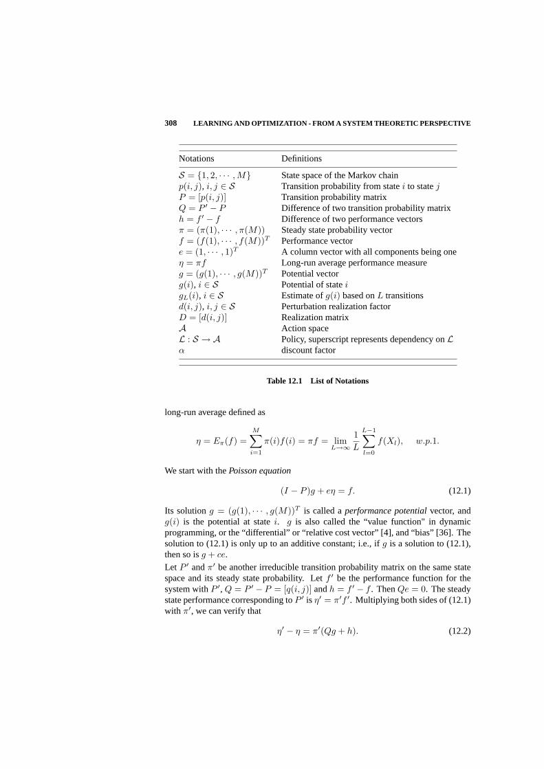
308 LEARNING AND OPTIMIZATION - FROM A SYSTEM THEORETIC PERSPECTIVE
Notations Definitions
S = 1, 2, · · · ,M State space of the Markov chainp(i, j), i, j ∈ S Transition probability from statei to statejP = [p(i, j)] Transition probability matrixQ = P ′ − P Difference of two transition probability matrixh = f ′ − f Difference of two performance vectorsπ = (π(1), · · · , π(M)) Steady state probability vectorf = (f(1), · · · , f(M))T Performance vectore = (1, · · · , 1)T A column vector with all components being oneη = πf Long-run average performance measureg = (g(1), · · · , g(M))T Potential vectorg(i), i ∈ S Potential of stateigL(i), i ∈ S Estimate ofg(i) based onL transitionsd(i, j), i, j ∈ S Perturbation realization factorD = [d(i, j)] Realization matrixA Action spaceL : S → A Policy, superscript represents dependency onLα discount factor
Table 12.1 List of Notations
long-run average defined as
η = Eπ(f) =M∑
i=1
π(i)f(i) = πf = limL→∞
1L
L−1∑
l=0
f(Xl), w.p.1.
We start with thePoisson equation
(I − P )g + eη = f. (12.1)
Its solutiong = (g(1), · · · , g(M))T is called aperformance potentialvector, andg(i) is the potential at statei. g is also called the “value function" in dynamicprogramming, or the “differential” or “relative cost vector” [4], and “bias” [36]. Thesolution to (12.1) is only up to an additive constant; i.e., ifg is a solution to (12.1),then so isg + ce.
Let P ′ andπ′ be another irreducible transition probability matrix on the same statespace and its steady state probability. Letf ′ be the performance function for thesystem withP ′, Q = P ′ − P = [q(i, j)] andh = f ′ − f . ThenQe = 0. The steadystate performance corresponding toP ′ is η′ = π′f ′. Multiplying both sides of (12.1)with π′, we can verify that
η′ − η = π′(Qg + h). (12.2)
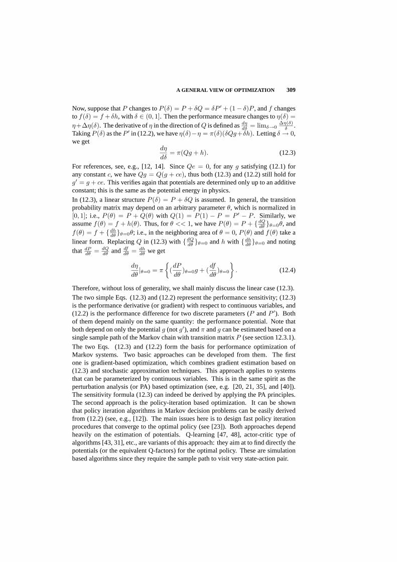
A GENERAL VIEW OF OPTIMIZATION 309
Now, suppose thatP changes toP (δ) = P + δQ = δP ′ + (1− δ)P , andf changesto f(δ) = f + δh, with δ ∈ (0, 1]. Then the performance measure changes toη(δ) =η+∆η(δ). The derivative ofη in the direction ofQ is defined asdη
dδ = limδ→0∆η(δ)
δ .TakingP (δ) as theP ′ in (12.2), we haveη(δ)−η = π(δ)(δQg+δh). Lettingδ → 0,we get
dη
dδ= π(Qg + h). (12.3)
For references, see, e.g., [12, 14]. SinceQe = 0, for any g satisfying (12.1) forany constantc, we haveQg = Q(g + ce), thus both (12.3) and (12.2) still hold forg′ = g + ce. This verifies again that potentials are determined only up to an additiveconstant; this is the same as the potential energy in physics.
In (12.3), a linear structureP (δ) = P + δQ is assumed. In general, the transitionprobability matrix may depend on an arbitrary parameterθ, which is normalized in[0, 1]; i.e., P (θ) = P + Q(θ) with Q(1) = P (1) − P = P ′ − P . Similarly, weassumef(θ) = f + h(θ). Thus, forθ << 1, we haveP (θ) = P + dQ
dθ θ=0θ, andf(θ) = f + dh
dθ θ=0θ; i.e., in the neighboring area ofθ = 0, P (θ) andf(θ) take alinear form. ReplacingQ in (12.3) withdQ
dθ θ=0 andh with dhdθ θ=0 and noting
that dPdθ = dQ
dθ and dfdθ = dh
dθ we get
dη
dθ|θ=0 = π
(dP
dθ)θ=0g + (
df
dθ)θ=0
. (12.4)
Therefore, without loss of generality, we shall mainly discuss the linear case (12.3).
The two simple Eqs. (12.3) and (12.2) represent the performance sensitivity; (12.3)is the performance derivative (or gradient) with respect to continuous variables, and(12.2) is the performance difference for two discrete parameters (P andP ′). Bothof them depend mainly on the same quantity: the performance potential. Note thatboth depend on only the potentialg (notg′), andπ andg can be estimated based on asingle sample path of the Markov chain with transition matrixP (see section 12.3.1).
The two Eqs. (12.3) and (12.2) form the basis for performance optimization ofMarkov systems. Two basic approaches can be developed from them. The firstone is gradient-based optimization, which combines gradient estimation based on(12.3) and stochastic approximation techniques. This approach applies to systemsthat can be parameterized by continuous variables. This is in the same spirit as theperturbation analysis (or PA) based optimization (see, e.g. [20, 21, 35], and [40]).The sensitivity formula (12.3) can indeed be derived by applying the PA principles.The second approach is the policy-iteration based optimization. It can be shownthat policy iteration algorithms in Markov decision problems can be easily derivedfrom (12.2) (see, e.g., [12]). The main issues here is to design fast policy iterationprocedures that converge to the optimal policy (see [23]). Both approaches dependheavily on the estimation of potentials. Q-learning [47, 48], actor-critic type ofalgorithms [43, 31], etc., are variants of this approach: they aim at to find directly thepotentials (or the equivalent Q-factors) for the optimal policy. These are simulationbased algorithms since they require the sample path to visit very state-action pair.

310 LEARNING AND OPTIMIZATION - FROM A SYSTEM THEORETIC PERSPECTIVE
12.3 ESTIMATION OF POTENTIALS AND PERFORMANCEDERIVATIVES
As shown in section 12.2, potentials and the two sensitivity formulas (12.2) and (12.3)play a crucial role in performance optimization. we first present in section 12.3.1some on-line algorithms for estimating potentials (or formulas based on which suchalgorithms can be easily derived). To overcome the well-known difficulty of largestate space, we observe that with (12.3) it is possible to estimate performance deriva-tives directly without estimating the potentials for all the states. This is discussedin section 12.3.2. We first propose a basic equation for gradient estimation (12.18).Three different techniques developed by different authors for estimating gradientsare presented as special cases of (12.18). Other algorithms can also be developed.Section 12.3.3 provides a historical view of the performance gradient estimation,early works on perturbation analysis (PA) and the likelihood ratio (LR) methods arediscussed.
12.3.1 Estimation of Performance Potentials
We first show that the potentials of a Markov chain can be estimated with a singlesample path of the Markov chain. Sinceg is only up to an additive constant, we maychoose the one that satisfiesπg = πf = η. Thus, (12.1) becomes
(I − P + eπ)g = f. (12.5)
For ergodic chains,I − P + eπ is invertible; thus,
g = (I − P + eπ)−1f =∞∑
l=0
(P − eπ)lf
= I +∞∑
k=1
(P kf − ηe). (12.6)
Consider a sample path of the Markov chain, denoted asX = X0, X1, · · · , Xn, · · · .Ignoring the constantηe in (12.6), we have
g(i) = E∞∑
k=0
[f(Xk)− η]|X0 = i, (12.7)
which can be approximated by (with a large integerL)
gL(i) ≈ E[L−1∑
l=0
f(Xl)|X0 = i]− Lη. (12.8)
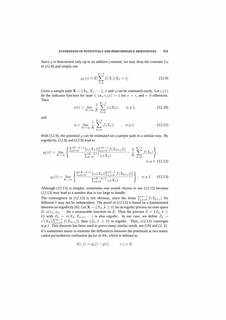
ESTIMATION OF POTENTIALS AND PERFORMANCE DERIVATIVES 311
Sinceg is determined only up to an additive constant, we may drop the constantLηin (12.8) and simply use
gL(i) ≈ E[L−1∑
l=0
f(Xl)|X0 = i]. (12.9)
Given a sample pathX = X0, X1, · · · , π andη can be estimated easily. Letεi(x)be the indicator function for statei; i.e., εi(x) = 1 for x = i, and= 0 otherwise.Then
π(i) = limK→∞
1K
K−1∑
k=0
εi(Xk), w.p.1, (12.10)
and
η = limK→∞
1K
K−1∑
k=0
f(Xk), w.p.1. (12.11)
With (12.9), the potentialg can be estimated on a sample path in a similar way. Byergodicity, (12.8) and (12.9) lead to
gL(i) = limK→∞
∑K−L+1k=0 εi(Xk)[
∑L−1j=0 f(Xk+j)]∑K−L+1
k=0 εi(Xk)− L
K
K−1∑
k=0
f(Xk)
,
w.p.1. (12.12)
gL(i) = limK→∞
∑K−L+1k=0 εi(Xk)[
∑L−1j=0 f(Xk+j)]∑K−L+1
k=0 εi(Xk)
, w.p.1. (12.13)
Although (12.13) is simpler, sometimes one would choose to use (12.12) because(12.13) may lead to a number that is too large to handle.
The convergence in (12.13) is not obvious, since the items∑n−1
j=0 f(Xk+j) fordifferentk may not be independent. The proof of (12.13) is based on a fundamentaltheorem on ergodicity [6]: LetX = Xk, k ≥ 0 be an ergodic process on state spaceS; φ(x1, x2, · · · )be a measurable function onS. Then the processZ = Zk, k ≥0 with Zk = φ(Xk, Xk+1, · · · ) is also ergodic. In our case, we defineZk =εi(Xk)[
∑n−1j=0 f(Xk+j)]; then Zk, k ≥ 0 is ergodic. Thus, (12.13) converges
w.p.1. This theorem has been used to prove many similar result, see [19] and [2, 3].
It’s sometimes easier to estimate the differences between the potentials at two states,calledperturbation realization factorin PA, which is defined as
d(i, j) = g(j)− g(i), i, j ∈ S.
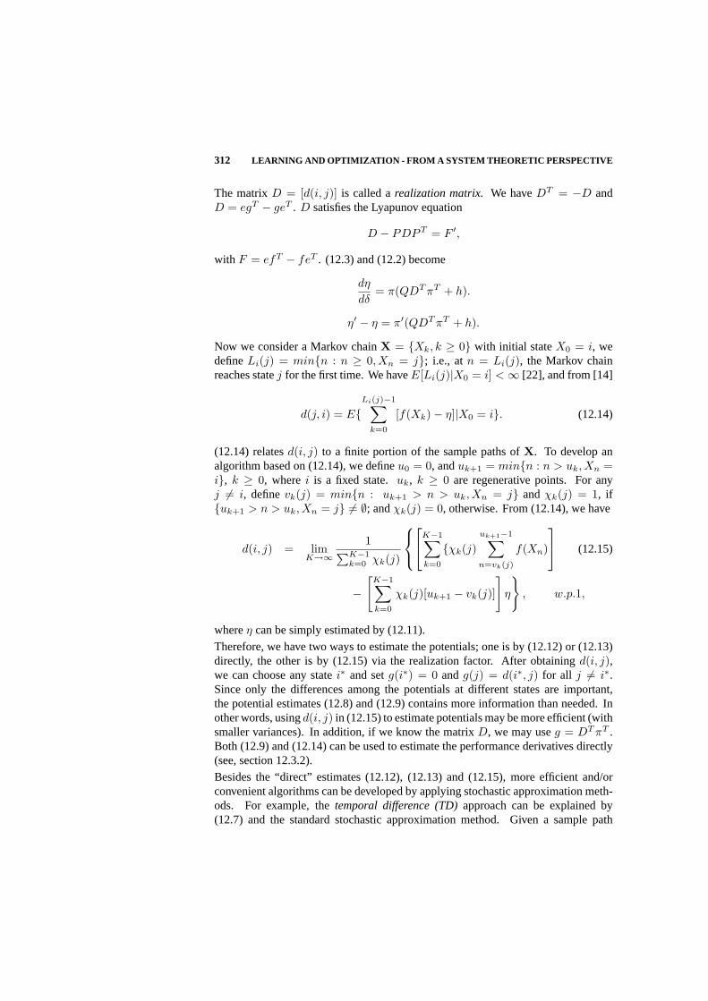
312 LEARNING AND OPTIMIZATION - FROM A SYSTEM THEORETIC PERSPECTIVE
The matrixD = [d(i, j)] is called arealization matrix. We haveDT = −D andD = egT − geT . D satisfies the Lyapunov equation
D − PDPT = F ′,
with F = efT − feT . (12.3) and (12.2) become
dη
dδ= π(QDT πT + h).
η′ − η = π′(QDT πT + h).
Now we consider a Markov chainX = Xk, k ≥ 0 with initial stateX0 = i, wedefineLi(j) = minn : n ≥ 0, Xn = j; i.e., atn = Li(j), the Markov chainreaches statej for the first time. We haveE[Li(j)|X0 = i] < ∞ [22], and from [14]
d(j, i) = ELi(j)−1∑
k=0
[f(Xk)− η]|X0 = i. (12.14)
(12.14) relatesd(i, j) to a finite portion of the sample paths ofX. To develop analgorithm based on (12.14), we defineu0 = 0, anduk+1 = minn : n > uk, Xn =i, k ≥ 0, wherei is a fixed state.uk, k ≥ 0 are regenerative points. For anyj 6= i, definevk(j) = minn : uk+1 > n > uk, Xn = j andχk(j) = 1, ifuk+1 > n > uk, Xn = j 6= ∅; andχk(j) = 0, otherwise. From (12.14), we have
d(i, j) = limK→∞
1∑K−1k=0 χk(j)
K−1∑
k=0
χk(j)uk+1−1∑
n=vk(j)
f(Xn)
(12.15)
−[
K−1∑
k=0
χk(j)[uk+1 − vk(j)]
]η
, w.p.1,
whereη can be simply estimated by (12.11).
Therefore, we have two ways to estimate the potentials; one is by (12.12) or (12.13)directly, the other is by (12.15) via the realization factor. After obtainingd(i, j),we can choose any statei∗ and setg(i∗) = 0 andg(j) = d(i∗, j) for all j 6= i∗.Since only the differences among the potentials at different states are important,the potential estimates (12.8) and (12.9) contains more information than needed. Inother words, usingd(i, j) in (12.15) to estimate potentials may be more efficient (withsmaller variances). In addition, if we know the matrixD, we may useg = DT πT .Both (12.9) and (12.14) can be used to estimate the performance derivatives directly(see, section 12.3.2).
Besides the “direct” estimates (12.12), (12.13) and (12.15), more efficient and/orconvenient algorithms can be developed by applying stochastic approximation meth-ods. For example, thetemporal difference (TD)approach can be explained by(12.7) and the standard stochastic approximation method. Given a sample path

ESTIMATION OF POTENTIALS AND PERFORMANCE DERIVATIVES 313
X0, · · · , Xn, Xn+1, · · · , , at thenth transition, we have
g(Xn) = E∞∑
k=0
[f(Xn+k)− η]|Xn = [f(Xn)− η] + E[g(Xn+1)|Xn]. (12.16)
Now suppose we observe a transition from stateXn toXn+1. If g(Xn) is the estimateat timen, then[f(Xn)− η]+ g(Xn+1) may be a more accurate estimate thang(Xn)because it reflects the information at this transition. Define thetemporal difference(TD) as
dn = [f(Xn)− η + g(Xn+1)− g(Xn)],
which may represent the stochastic error observed at transitionn. Based on (12.16)and with the stochastic approximation approach, some recursive on-line algorithms(called TD(λ) algorithms) for estimatingg(i) can be developed. [44, 46] presentsTD(λ) algorithms with linearly parameterized function approximation. For TD (λ)algorithms for discounted or total cost problems, see [5, 45, 41, 42].
In addition to the above approaches,neuro-dynamic programmingis proposed toovercome the difficulty of the so-called “curse of dimensionality”. Roughly speaking,in neuro-dynamic programming, we try to approximate the potential functiong(i) byg(i, r), with a continuous parameterr. This generally involves two steps:
1. develop an approximation architecture, e.g., a neuro-network, to representg(i, r),
2. find a training algorithm for updating the parameter vectorr, based on theinformation observed on a sample path.
After training, the parameterr reaches a proper value. The neuro-network willoutput an approximate value ofg(i) for an input integeri. For details and successfulexamples, see [5].
12.3.2 Gradient Estimation
There are two ways in estimating the performance measureη: we may estimateall π(i) by (12.10) first and then useη = πf to calculate the performance, or wemay estimateη directly by (12.11). The situation is similar for the performancederivatives: we may first estimateg by the methods presented in section 12.3.1, thenobtain the derivatives by (12.3), or we may estimateπQg directly. The disadvantageof the former is that the state space is usually too large. In the following, we presenta few “direct” algorithms forπQg (similar to (12.11) forη).
Consider a stationary Markov chainX = (X0, X1, · · · , ). (This implies the initialprobability distribution isπ.) Let E denote the expectation on the probability spacegenerated byX. Denote a generic time instant ask. Because it is impossible fora sample path withP to contain information aboutP ′, we need to use a standard

314 LEARNING AND OPTIMIZATION - FROM A SYSTEM THEORETIC PERSPECTIVE
technique in simulation calledimportance sampling. We have
dη
dδ= π(Qg + h) =
∑
i∈S
∑
j∈Sπ(i)[p(i, j)
q(i, j)p(i, j)
g(j) + h(i)]
= E
q(Xk, Xk+1)p(Xk, Xk+1)
g(Xk+1) + h(Xk)
. (12.17)
Furthermore, ifg is a random variable defined onX such thatE(g) = g and g isindependent of the transition fromXk to Xk+1, then we have
dη
dδ= E
q(Xk, Xk+1)p(Xk, Xk+1)
g(Xk+1) + h(Xk)
. (12.18)
Eq. (12.18) is the fundamental equation for performance gradient estimation. Samplepath based algorithms can be developed by using (12.18) and any estimate ofg. Inthe following, we present three different techniques based on (12.18).
The first algorithm is based on (12.9). From (12.9), we can choose
g(X0) :=L−1∑
l=0
f(Xl).
Using thisg in (12.18) (for simplicity, we seth = 0), we have
∂η
∂δ= E
q(Xk, Xk+1)p(Xk, Xk+1)
[L−1∑
l=0
f(Xk+l+1)] + h(Xk)
= limK→∞
1K − L + 1
K−L∑
k=0
q(Xk, Xk+1)p(Xk, Xk+1)
[L−1∑
l=0
f(Xk+l+1)]
, w.p.1.
(12.19)
This equation is similar to (12.13) with one modification: a modifying factorq(Xk,Xk+1)p(Xk,Xk+1)
is multiplied to the term∑L−1
l=0 f(Xk+l+1). It can be shown that (12.19)is equivalent to [19]
∂η
∂δ≈ lim
K→∞1
K − L + 1
K−L∑
k=0
f(Xk+L)
L−1∑
l=0
[q(Xk+l, Xk+l+1)p(Xk+l, Xk+l+1)
], w.p.1.
(12.20)
In (12.19) and (12.20),g is approximated by truncation. In the second algorithm,we use anα-potentialgα, 0 < α < 1, to approximateg. gα satisfies the followingdiscounted Poisson equation [15]:
(I − αP + αeπ)gα = f.
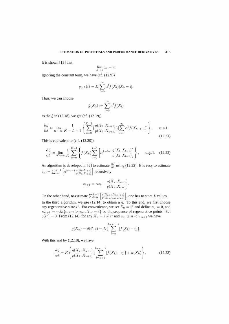
ESTIMATION OF POTENTIALS AND PERFORMANCE DERIVATIVES 315
It is shown [15] thatlimα→1
gα = g.
Ignoring the constant term, we have (cf. (12.9))
gα,L(i) = E[∞∑
l=0
αlf(Xl)|X0 = i].
Thus, we can choose
g(X0) :=∞∑
l=0
αlf(Xl)
as theg in (12.18), we get (cf. (12.19))
∂η
∂δ≈ lim
K→∞1
K − L + 1
K−L∑
k=0
q(Xk, Xk+1)p(Xk, Xk+1)
[∞∑
l=0
αlf(Xk+l+1)]
, w.p.1.
(12.21)This is equivalent to (c.f. (12.20))
∂η
∂δ≈ lim
K→∞1K
K−1∑
k=0
f(Xk)
k−1∑
l=0
[αk−l−1 q(Xl, Xl+1)
p(Xl, Xl+1)
], w.p.1. (12.22)
An algorithm is developed in [2] to estimate∂η∂δ using (12.22). It is easy to estimate
zk :=∑k−1
l=0
[αk−l−1 q(Xl,Xl+1)
p(Xl,Xl+1)
]recursively:
zk+1 = αzk +q(Xk, Xk+1)p(Xk, Xk+1)
.
On the other hand, to estimate∑L−1
l=0
[q(Xk+l,Xk+l+1)p(Xk+l,Xk+l+1)
], one has to storeL values.
In the third algorithm, we use (12.14) to obtain ag. To this end, we first chooseany regenerative statei∗. For convenience, we setX0 = i∗ and defineu0 = 0, andum+1 = minn : n > um, Xm = i be the sequence of regenerative points. Setg(i∗) = 0. From (12.14), for anyXn = i 6= i∗ andum ≤ n < um+1 we have
g(Xn) = d(i∗, i) = Etm+1−1∑
l=n
[f(Xl)− η].
With this and by (12.18), we have
dη
dδ= E
q(Xk, Xk+1)p(Xk, Xk+1)
tm+1−1∑
l=k+1
[f(Xl)− η]+ h(Xk)
. (12.23)
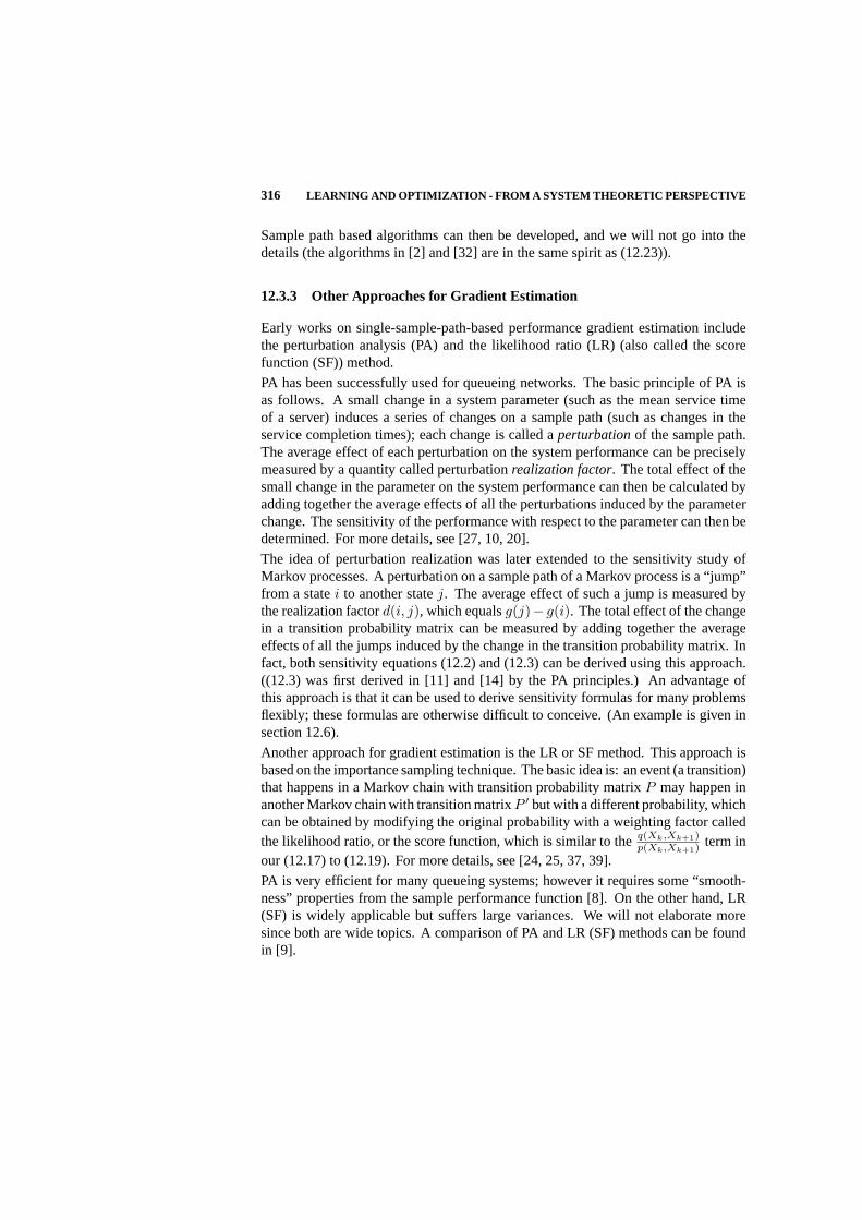
316 LEARNING AND OPTIMIZATION - FROM A SYSTEM THEORETIC PERSPECTIVE
Sample path based algorithms can then be developed, and we will not go into thedetails (the algorithms in [2] and [32] are in the same spirit as (12.23)).
12.3.3 Other Approaches for Gradient Estimation
Early works on single-sample-path-based performance gradient estimation includethe perturbation analysis (PA) and the likelihood ratio (LR) (also called the scorefunction (SF)) method.
PA has been successfully used for queueing networks. The basic principle of PA isas follows. A small change in a system parameter (such as the mean service timeof a server) induces a series of changes on a sample path (such as changes in theservice completion times); each change is called aperturbationof the sample path.The average effect of each perturbation on the system performance can be preciselymeasured by a quantity called perturbationrealization factor. The total effect of thesmall change in the parameter on the system performance can then be calculated byadding together the average effects of all the perturbations induced by the parameterchange. The sensitivity of the performance with respect to the parameter can then bedetermined. For more details, see [27, 10, 20].
The idea of perturbation realization was later extended to the sensitivity study ofMarkov processes. A perturbation on a sample path of a Markov process is a “jump”from a statei to another statej. The average effect of such a jump is measured bythe realization factord(i, j), which equalsg(j)− g(i). The total effect of the changein a transition probability matrix can be measured by adding together the averageeffects of all the jumps induced by the change in the transition probability matrix. Infact, both sensitivity equations (12.2) and (12.3) can be derived using this approach.((12.3) was first derived in [11] and [14] by the PA principles.) An advantage ofthis approach is that it can be used to derive sensitivity formulas for many problemsflexibly; these formulas are otherwise difficult to conceive. (An example is given insection 12.6).
Another approach for gradient estimation is the LR or SF method. This approach isbased on the importance sampling technique. The basic idea is: an event (a transition)that happens in a Markov chain with transition probability matrixP may happen inanother Markov chain with transition matrixP ′ but with a different probability, whichcan be obtained by modifying the original probability with a weighting factor calledthe likelihood ratio, or the score function, which is similar to theq(Xk,Xk+1)
p(Xk,Xk+1)term in
our (12.17) to (12.19). For more details, see [24, 25, 37, 39].
PA is very efficient for many queueing systems; however it requires some “smooth-ness” properties from the sample performance function [8]. On the other hand, LR(SF) is widely applicable but suffers large variances. We will not elaborate moresince both are wide topics. A comparison of PA and LR (SF) methods can be foundin [9].

GRADIENT-BASED OPTIMIZATION 317
12.4 GRADIENT-BASED OPTIMIZATION
Any gradient estimate (PA, LR or SF, or the potential based estimates discussed insection 12.3) can be used together with the standard stochastic gradient algorithms(Robbins-Monroe type, [38]) for optimizing the performance of Markov systems.For applications of PA and LR to the optimization problems, see e.g., [26, 21] and[25], respectively.
[32] proposed a potential-based recursive algorithm for optimizing the average cost infinite state Markov reward processes that depend on a set of parameters denoted asθ.The approach is based on the regenerative structure of a Markov chain. The gradientestimate is similar to (12.23) except that the performanceη is also estimated on thesample path and the gradient is not estimated explicitly in each step of the recursion,because its estimate is used in the stochastic gradient algorithm to determine the stepsize in a recursive procedure to reach the valueθ at which the performance gradient iszero. The paper also provides a proof for the convergence of the algorithm. Variancereduction methods are proposed in [33].
The gradient based approach can be easily extended to the partially observableMarkov decision processes (POMDP) (see, e.g., [2, 3]). The POMDP model in[2, 3] is described as follows. In addition to the state spaceS = 1, · · · ,M,there is a control space denoted asU = 1, · · · , N consisting ofN controls andan observation spaceY = 1, · · · , L consisting ofL observations. Eachu ∈U determines a transition probability matrixPu, which does not depend on theparameterθ. When the Markov chain is at statei ∈ S, an observationy ∈ Y isobtained according to a probability distributionνi(y). For any observationy, wemay choose a random policyµy(u), which is a probability distribution over thecontrol spaceU . It is assumed that the distribution depends on the parameterθ andtherefore is denoted asµy(θ, u).Given an observation distributionνi(y) and a random policyµy(θ, u), the corre-sponding transition probabilities are
pθ(i, j) =∑u,y
νi(y)µy(θ, u)pu(i, j).
Therefore,d
dθpθ(i, j) =
∑u,y
νi(y)pu(i, j)d
dθµy(θ, u). (12.24)
In POMDP, we assume that although the stateXk, k = 0, 1, · · · , is not completelyobservable, the costf(Xk) is known. Thus, algorithms can be developed by replacingq(i, j) with d
dθ pθ(i, j) of (12.24) in the algorithms developed for standard MDPs insection 12.3.2. For example, ifh(i) = 0 then (12.23) becomes
dη
dδ= E
ddθ pθ(Xk, Xk+1)p(Xk, Xk+1)
tm+1−1∑
l=k+1
[f(Xl)− η]
,

318 LEARNING AND OPTIMIZATION - FROM A SYSTEM THEORETIC PERSPECTIVE
in whichf(Xk) is assumed to be observable.
A recursive algorithm called GPOMDP is presented in [2]. The algorithm uses adiscount factor to approximateg (cf. (12.22)).
12.5 POLICY ITERATION
Policy iteration procedure in MDPs is a natural consequence of the performancedifference equation (12.2). First, for twoM -dimensional vectorsa andb, we definea = b if a(i) = b(i) for all i = 1, 2 · · · ,M ; a ≤ b if a(i) < b(i) or a(i) = b(i)for all i = 1, 2 · · · , M ; a < b if a(i) < b(i) for all i = 1, 2 · · · ,M ; anda ¹ b ifa(i) < b(i) for at least onei, anda(j) = b(j) for other components. The relation≤includes=,¹, and<. Similar definitions are used for the relations>,º, and≥.
Next, we note thatπ′(i) > 0, ∀i, for ergodic chains. Thus, from (12.2), we knowthat if Qg + h = (P ′ − P )g + (f ′ − f) º 0 thenη′ − η > 0. Thus, we have
Lemma 12.5.1 If Pg + f ¹ P ′g + f ′, thenη < η′.
In an MDP, at any transition instantn ≥ 0 of a Markov chainX = Xn, n ≥ 0,an action is chosen from an action spaceA and is applied to the Markov chain.We assume that the number of actions is finite, and we only consider stationarypolicies. A stationary policy is a mappingL : S → A, i.e., for any statei, Lspecifies an actionL(i) ∈ A. Let E be the policy space. If actionα is takenat statei, then the state transition probabilities at statei are denoted aspα(i, j),j = 1, 2, · · · , M . With a policyL, the Markov process evolves according to thetransition matrixPL = [pL(i)(i, j)]Mi=1|Mj=1. We use the superscript∗L to denote thequantities associated with policyL.
The cost depends on action and is denoted asf(i, α) = f(i,L(i)). The long-runaverage performance isηL. Our objective is to minimize this average cost over thepolicy spaceS, i.e., to obtainminL∈E ηL.
DefinefL = (f [1,L(1)], · · · , f [M,L(M)])T . (12.5) becomes
(I − PL + eπL)gL = fL, (12.25)
The following optimality theorem follows almost immediately from Lemma 12.5.1.
Theorem 12.5.1A policyL is optimal if and only if
PLgL + fL ≤ PL′gL + fL
′(12.26)
for all L′ ∈ E .
The optimality condition (12.26) is, of course, equivalent to the other conditions inthe literature. To see this, we rewrite (12.25) in the following form:
ηLe + gL = fL + PLgL. (12.27)

POLICY ITERATION 319
Then Theorem 12.5.1 becomes: A policyL is optimal if and only if
ηLe + gL = minL′∈E
PL′gL + fL′. (12.28)
The minimum is taken for every component of the vector. (12.28) is the optimalityequation, or the Bellman equation.
Policy iteration algorithms for determining the optimal policy can be easily developedby combining Lemma 12.5.1 and Theorem 12.5.1. Roughly speaking, at thekth stepwith policyLk, we set the policy for the next step (the(k + 1)th step) as
Lk+1 = argmin[PLgLk + fL], (componentwise), (12.29)
with gLk being the solution to the Poisson equation forPLk . Lemma 12.5.1 impliesthat performance usually improves at each iteration. Theorem 12.5.1 shows that theminimum is reached when no performance improvement can be achieved. We shallnot state the details here because they are standard. The extension of the above resultsto multi-chain Markov chains is presented in [18].
12.5.1 On-line Policy Iteration Algorithms
With the potentials estimated, we can implement policy iteration to obtain the optimalpolicy. The simplest way is that at each iterationk we run the system under policyLk long enough to get an accurate estimate ofgLk , then determine the policy in thenext iteration using (12.29) until no improvement can be made [13]. This approachrequires a long sample path at each iteration. However, in order to make comparisonof two policies to determine which one is better using (12.2), some errors in estimationare tolerable. This is especially true at the beginning of the iteration procedure sincethe performance is far from the optimum. (A precise study of this idea is formulatedin the “ordinal optimization” approach, see [28]). Therefore, fast algorithms can bedesigned by combining the policy iteration method with stochastic approximation,with “rough” estimates of potentials at the beginning of the iterations.
[23] proposes two such on-line optimization algorithms that implement policy it-eration based on a sample path. In these algorithms, estimates of potentials areupdated when the system visits a certain recurrent state. Since the policies are up-dated frequently, the potential estimates may reflect the values under the previouspolicies; thus, well-designed stochastic approximation schemes are used to guaranteethe convergence of the policies to the optimal one. The difference between the twoalgorithms is that in one algorithm the entire policy is updated when the estimates ofthe potentials are made, and in the other the action for a particular state is updatedonly when the system visits the state. It is proved in the paper that starting fromany initial value, the policy sequences obtained by these two algorithms will stop atthe optimal one after a finite number of iterations. The on-line policy iteration ap-proach is a counterpart of the online gradient based optimization approach presented

320 LEARNING AND OPTIMIZATION - FROM A SYSTEM THEORETIC PERSPECTIVE
in section 12.4; the latter applies to parameterized systems and the former to systemswithin the MDP general structure.
12.5.2 Gradient-Based Policy Iteration
Comparing (12.2) with (12.3), we have the following observations [12, 17]:
1. The performance difference of any two policiesP andP ′ (12.2) can be obtainedby replacingπ with π′ in the formula for the performance derivative (12.3).For anyP ′ (or anyQ = P ′ − P ) andh, the performance derivative can becalculated by solving forπ andg for the system withP . But for performancedifference,π′ is needed for eachP ′.
2. At each iteration, one chooses the policy with the largest|Qg +h|, componen-twise, as the policy in the next iteration. That is, policy iteration goes along thedirection with the steepest performance gradient (with the largest|π(Qg+h)|).
3. Sinceπ′ is usually unknown, policy iteration must determine actions state bystate; therefore, it does not apply to systems in which actions at different statesare correlated. On the other hand,π is known at each iteration, we can calculateperformance derivatives even when actions at some states are correlated.
With the above observations, [17] proposes a gradient-based policy iteration thatmay be applied to systems with correlated actions at different states. We treat theproblem as performance optimization in a policy space with constraints for policies.The main idea is to iterate the policy along the steepest direction in the constrainedregion. However, there are some theoretical issues remaining. For example, theproposed approach may lead to a policy that is locally optimal, i.e., at this point allthe directional gradients to other policies are non-negative (in case of performanceminimization). In addition, the convergence of the algorithms have to be proved.
The idea is best illustrated with an example. Consider an M/G/1/N queue, in whichthe service distribution is a Coxian distribution consisting ofK stages, each isexponentially distributed with meansi, i = 1, 2, · · · ,K (K = 3 in Figure 12.1). (Forqueueing theory, see [30].) After receiving service at stagek, a customer enters stagek+1 with probabilityak, and leaves the station with probabilitybk = 1−ak, aK = 0.Letn be the number of customers in the queue.N is the buffer size: when an arrivingcustomer findsn = N , the customer is simply lost. Customers arrive with a Poissonprocess with rateλ. When there aren customers in the queue and the customer isserved at stagek, an arriving customer has a probability ofσ(n, k) joining the queue,and1− σ(n, k) being rejected (the admission control problem);σ(N, k) = 0 for allk. This is equivalent to a load-dependent arrival rateλ(n, k) = λσ(n, k). The statespace of the system is0, (n, k), n = 1, 2, · · · , N, k = 1, 2, · · · ,K. The actionspace is the set of values thatσ(n, k) may take; e.g., in the numerical example in[17], it is the set0.1, 0.2, · · · 0.9.

POLICY ITERATION 321
½¼
¾»
½¼
¾»
½¼
¾»- - -
a1 a2
b3b1 b2
s1 s2 s3λσ(n, k)
1− σ(n, k)
n
??? -
-?
Fig. 12.1 An M/G/1/N Queue Admission Control
Since the stagek is usually not observable, it is not feasible to implement a policythat depends onk. Denote the action asσ(n, s) then we have the constraint
σ(n, 1) = σ(n, 2) = σ(n, 3) ≡ σ(n). (12.30)
“n” is an “aggregated” state.
The problem can be converted to a discrete time MDP by uniformization. In thenumerical example in [17], the cost function is set asf(n, λ(n, k)) = n2 + 9 ×(1/λσ(n, k))2. Indeed, the standard policy iteration leads to an optimal policy whichassigns different actions for different stages with the samen, which is not practicallyimplementable.
To implement the gradient-based policy iteration, we need to calculate the perfor-mance gradient in the constraint policy space. In this example, letσ0 be the currentpolicy andσ be any other policy. Then the derivative alongσ0 to σ is
dη
dδ=
N∑n=0
K∑
i=1
πσ0(n, i)[
∑
m,j
pσ[(n, i), (m, j)]
−pσ0 [(n, i), (m, j)]gσ0(m, j) + (fσ(n, i)− fσ0(n, i))] .(12.31)
Defining a “W-factor” (cf. Q-factor)
W (n, σ(n)) ≡K∑
i=1
πσ0(n, i)
∑
m,j
pσ[(n, i), (m, j)]gσ0(m, j)+ fσ(n, i)
,
(12.32)we have
dη
dδ=
N∑n=0
W (n, σ(n))−W (n, σ0(n)). (12.33)
For eachn, W (n, σ(n))−W (n, σ0(n)) is called apartial derivative.
From the above discussion, with the current policyσ0, we can calculate the W-factorfor any actionσ(n) (for each aggregated state). Thus, for anyn we can choose anaction with the smallest value of the W-factor (12.32), or equivalently the “steepest”

322 LEARNING AND OPTIMIZATION - FROM A SYSTEM THEORETIC PERSPECTIVE
partial derivative. From (12.33) we can get a policy having the steepest gradient andyet satisfying constraint (12.30). Using this policy as the policy in the next iteration,we can carry out policy iteration. Indeed, the numerical example in [17] shows thatthis procedure does stop at a feasible policy whose performance is very close tothe one obtained by the standard policy iteration procedure (i.e., the optimal policywithout the constraint (12.30)).
12.6 CONSTRUCTING PERFORMANCE GRADIENTS WITHPOTENTIALS AS BUILDING BLOCKS
We have seen that potentials are the central piece in the performance sensitivity(difference and derivative) formulas. In fact, it can be shown that we can usepotentials as building blocks to construct freely performance sensitivities for manyspecial problems (see [16]). This “construction” approach is based on the followingfundamental principle: changes in the values of system parameters induce “jumps”on a sample path; the effect of a jump from statei to j can be measured by therealization factorsd(i, j) = g(j) − g(i). In [16], it is shown that both (12.2) and(12.3) can be constructed in this way.
In this section, we use an example to show one application of this approach. Specif-ically, we show that in systems where only a part of the states is observable, we canaggregate the potentials on a set of states that share the same observable part of statesand obtain the performance gradients. The aggregated potential can be estimated ona single sample path.
Consider the M/G/1/N queue shown in Figure 12.1. For illustrative purpose, weassume that the queue consists ofK stages, all with the same meansk ≡ s, k =1, 2, · · · ,K. Let µ = 1
s .
We are interested in the performance gradient with respect toσ(n), for a givenn,n = 0, 1, · · · , N − 1. One way to get this gradient is to use (12.3); however, thisrequires us to model the system as a Markov chain and to estimate the potentialsfor all the states; many of the states may not be affected by the changes inσ(n).In the following, we shall show that this gradient can be constructed directly byusing potentials (or equivalently, realization factors) as building blocks without goingthrough the standard Markov model. To illustrate the idea, we setλ = µ (assumeµ > λσ(n) for all n). With uniformization, we generate a Poisson process with rateλ + Kµ = (K + 1)λ, a point on this Poisson process is assigned to be the servicecompletion time of one of the stages of the Coxian distribution or a customer arrivalpoint with probability λ
λ+Kµ = 1K+1 . When there aren customers in the system,
with probabilityσ(n), the arriving customer is accepted and the number of customersin the system increases ton+1, and with probability1−σ(n), the arriving customeris rejected and the number of customers in the system remains to ben. Let thediscretized Markov chain be denoted asX = X0, X1, · · · , Xl, · · · .We observe the system for a total ofL >> 1 transitions and obtainX0, X1, · · · , XL.Let p(n) be the probability that a transition on the sample path is due to a customer
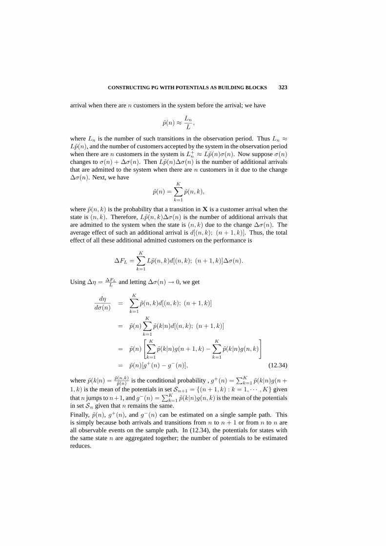
CONSTRUCTING PG WITH POTENTIALS AS BUILDING BLOCKS 323
arrival when there aren customers in the system before the arrival; we have
p(n) ≈ Ln
L,
whereLn is the number of such transitions in the observation period. ThusLn ≈Lp(n), and the number of customers accepted by the system in the observation periodwhen there aren customers in the system isL+
n ≈ Lp(n)σ(n). Now supposeσ(n)changes toσ(n) + ∆σ(n). ThenLp(n)∆σ(n) is the number of additional arrivalsthat are admitted to the system when there aren customers in it due to the change∆σ(n). Next, we have
p(n) =K∑
k=1
p(n, k),
wherep(n, k) is the probability that a transition inX is a customer arrival when thestate is(n, k). Therefore,Lp(n, k)∆σ(n) is the number of additional arrivals thatare admitted to the system when the state is(n, k) due to the change∆σ(n). Theaverage effect of such an additional arrival isd[(n, k); (n + 1, k)]. Thus, the totaleffect of all these additional admitted customers on the performance is
∆FL =K∑
k=1
Lp(n, k)d[(n, k); (n + 1, k)]∆σ(n).
Using∆η = ∆FL
L and letting∆σ(n) → 0, we get
dη
dσ(n)=
K∑
k=1
p(n, k)d[(n, k); (n + 1, k)]
= p(n)K∑
k=1
p(k|n)d[(n, k); (n + 1, k)]
= p(n)
[K∑
k=1
p(k|n)g(n + 1, k)−K∑
k=1
p(k|n)g(n, k)
]
= p(n)[g+(n)− g−(n)], (12.34)
wherep(k|n) = p(n,k)p(n) is the conditional probability ,g+(n) =
∑Kk=1 p(k|n)g(n +
1, k) is the mean of the potentials in setSn+1 = (n + 1, k) : k = 1, · · · ,K giventhatn jumps ton+1, andg−(n) =
∑Kk=1 p(k|n)g(n, k) is the mean of the potentials
in setSn given thatn remains the same.
Finally, p(n), g+(n), andg−(n) can be estimated on a single sample path. Thisis simply because both arrivals and transitions fromn to n + 1 or from n to n areall observable events on the sample path. In (12.34), the potentials for states withthe same staten are aggregated together; the number of potentials to be estimatedreduces.
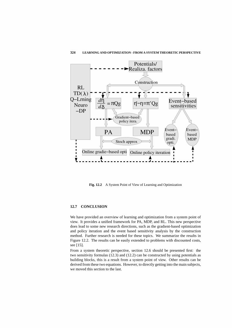
324 LEARNING AND OPTIMIZATION - FROM A SYSTEM THEORETIC PERSPECTIVE
’ ’Qg
λ
Realiza. factorsPotentials/
Event−
basedgradi.opti.
Event−
based
MDP
MDPPA
Stoch approx
Gradient−basedpolicy itera.
Online gradie−based opti
sensitivitiesEvent−based
Online policy iteration
Construction
δd= QgπdQ−Lrning η
RLTD( )
Neuro−DP
η−η=π
Fig. 12.2 A System Point of View of Learning and Optimization
12.7 CONCLUSION
We have provided an overview of learning and optimization from a system point ofview. It provides a unified framework for PA, MDP, and RL. This new perspectivedoes lead to some new research directions, such as the gradient-based optimizationand policy iteration and the event based sensitivity analysis by the constructionmethod. Further research is needed for these topics. We summarize the results inFigure 12.2. The results can be easily extended to problems with discounted costs,see [15].
From a system theoretic perspective, section 12.6 should be presented first: thetwo sensitivity formulas (12.3) and (12.2) can be constructed by using potentials asbuilding blocks, this is a result from a system point of view. Other results can bederived from these two equations. However, to directly getting into the main subjects,we moved this section to the last.

CONCLUSION 325
Acknowledgments
Supported in part by a grant from Hong Kong UGC. Tel: (852) 2358-7048; Fax: (852)2358-1485; Email: [email protected].

Bibliography
1. A. Arapostathis, V.S. Borkar, E. Fernandez-Gaucherand, M. K. Ghosh, andS. I. Marcus, “Discrete-Time Controlled Markov Processes with Average CostCriterion: A Survey,”SIAM J. Control and Optimization,Vol. 31, 282-344, 1993.
2. J. Baxter and P. L. Bartlett, “Infinite-Horizon Policy-Gradient Estimation,”Jour-nal of Artificial Intelligence Research,Vol. 15, 319-350, 2001.
3. J. Baxter, P. L. Bartlett, and L. Weaver “Experiments with Infinite-HorizonPolicy-Gradient Estimation,”Journal of Artificial Intelligence Research,Vol.15, 351-381, 2001.
4. D. P. Bertsekas,Dynamic Programming and Optimal Control,volume I and II.Athena Scientific, Belmont, MA, 1995.
5. D. P. Bertsekas and J. N. Tsitsiklis,Neuro-Dynamic Programming,Athena Sci-entific, Belmont, MA, 1996.
6. L. Breiman,Probability, Addison Wesly, 1968. Springer-Verlag, New York,1994.
7. P. Bremaud,Markov Chains: Gibbs Fields, Monte Carlo Simulation, andQueues,Springer-Verlag, New York, 1998.
8. X. R. Cao, “Convergence of Parameter Sensitivity Estimates in a StochasticExperiment,”IEEE Trans. on Automatic Control,Vol. AC- 30, 834-843, 1985.
9. X. R. Cao, “Sensitivity Estimates Based on One Realization of a StochasticSystem,”Journal of Statistical Computation and Simulation,Vol. 27, 211-232,1987.
10. X. R. Cao,Realization Probabilities: The Dynamics of Queueing Systems,Springer-Verlag, New York, 1994.
11. Xi-Ren Cao, X. M. Yuan, and L. Qiu, “A Single Sample Path-Based PerformanceSensitivity Formula for Markov Chains,”IEEE Transactions on Automatic Con-trol, Vol. 41, 1814-1817, 1996.
326

BIBLIOGRAPHY 327
12. X. R. Cao, “The Relation Among Potentials, Perturbation Analysis, MarkovDecision Processes, and Other Topics,“Journal of Discrete Event DynamicSystems,Vol. 8, 71-87, 1998.
13. X. R. Cao, “Single Sample Path Based Optimization of Markov Chains,”Journalof Optimization: Theory and Application,Vol.100, No.3, 527-548, 1999.
14. X. R. Cao and H. F. Chen, “Perturbation realization, potentials and sensitivityanalysis of Markov processes,”IEEE Trans. on Automat. Control,Vol. 42, 1382-1393, 1997.
15. X. R. Cao, “A Unified Approach to Markov Decision Problems and PerformanceSensitivity Analysis,”Automatica,Vol. 36, 771-774, 2000.
16. X. R. Cao, “Constructing Performance Sensitivities for Markov Systems withPotentials as Building Blocks,” submitted, 2003.
17. X. R. Cao and H. T. Fang, “Gradient-Based Policy Iteration: An Example,”Proceedings of 2002 IEEE Conference on Decision and Control,3367-3371,2002.
18. X. R. Cao and X. P. Guo, “A Unified Approach to Markov Decision Problemsand Sensitivity Analysis with Discounted and Average Criteria: the MultichainCase,” submitted.
19. X. R. Cao and Y.W. Wan, “Algorithms for sensitivity analysis of Markov systemsthrough potentials and perturbation realization,”IEEE Trans. on Control SystemTech,Vol. 6, 482-494, 1998.
20. C. G. Cassandras and S. Lafortune,Introduction to Discrete Event Systems,Kluwer Academic Publishers, 1999.
21. E. K. P. Chong and P. J. Ramadge, “Stochastic Optimization of RegenerativeSystems Using Infinitesimal Perturbation Analysis,”IEEE Trans. on Automat.Control,Vol. 39, 1400-1410, 1994.
22. E. Cinlar,Introduction to Stochastic Processes,Prentice Hall, Englewood cliffs,NJ, 1975.
23. Hai-Tao Fang and X. R. Cao, “Potential-Based On-line Policy Iteration Al-gorithms for Markov Decision Processes,”IEEE Transactions on AutomaticControl, to appear.
24. P. W. Glynn, “Likelihood Ratio Gradient Estimation: An Overview,”Proceedingsof 1987 Winter Simulation Conference,366-375, 1987.
25. P. W. Glynn, “Optimization of Stochastic Systems Via Simulation,”Proceedingsof 1987 Winter Simulation Conference,90-105, 1989.

328 BIBLIOGRAPHY
26. Y. C. Ho and X. R. Cao, “Perturbation Analysis and Optimization of QueueingNetworks,” Journal of Optimization Theory and Applications,40, 4, 559-582,1983.
27. Y. C. Ho and X. R. Cao,Perturbation Analysis of Discrete-Event DynamicSystems,Kluwer Academic Publisher, Boston, 1991.
28. L. H. Lee, E. T. K. Lau and Y. C. Ho, “Explanation of Goal Softening in OrdinalOptimization,”IEEE Trans. on Automat. Control,Vol. 44, 94-99, 1999.
29. T. Jaakkola, S. P. Singh, and M. I. Jordan, “Reinforcement Learning Algorithmfor Partially Observable Markov Decision Problems,”Advances in Neural Infor-mation Processing Systems,Vol. 7, 345-352, Morgan Kaufman, San Francisco,1995.
30. L. Kleinrock,Queueing Systems, Vol. 1: Theory,John Wiley, 1975.
31. V.R. Konda and V.S. Borkar, “Actor-ctritic- type Learning algorithms for Markovdecision processes,”SIAM J. Control Optim.,Vol. 38, 94-123, 1999.
32. P. Marbach and T. N. Tsitsiklis, “Simulation-based optimization of Markovreward processes,”IEEE Trans. on Automat. Control,Vol. 46, 191-209, 2001.
33. P. Marbach and T. N. Tsitsiklis, “Approximate Gradient Methods in Policy-SpaceOptimization of Markov Reward Processes,”Journal of Discrete Event DynamicSystems,l,to appear, 2002.
34. S. P. Meyn and R. L. Tweedie,Markov Chains and Stochastic Stability,Springer-Verlag, London, 1993.
35. E. L. Plambeck, B. R. Fu, S. M. Robinson, and R. Suri, “Sample-path optimiza-tion of convex stochastic performance functions,”Math. Program. B, Vol. 75,137-176, 1996.
36. M. L. Puterman,Markov Decision Processes: Discrete Stochastic DynamicProgramming,Wiley, New York, 1994.
37. M. I. Reiman and A. Weiss, “Sensitivity Analysis via Likelihood Ratio,”Oper-ations Research,Vol. 37, 830-844, 1989.
38. H. Robbins and S. Monro, “A Stochastic Approximation Method,”Annals ofMathematical Statistics,Vol. 22, 400-407, 1951.
39. R. V. Rubinstein,Monte Carlo Optimization, Simulation, and Sensitivity Analysisof Queueing Networks,Wiley, New York, 1986.
40. R. Suri and Y. T. Leung, “Single Run Optimization of Discrete Event Simulations- An Empirical Study Using the M/M/1 Queue,”IIE Transactions,Vol. 21, 35-49,1989.
BIBLIOGRAPHY 329
41. R. S. Sutton, “Learning to Predict by the Methods of Temporal Differences,”Machine Learning,Vol. 3, 835-846, 1988.
42. R. S. Sutton and A. G. Barto,Reinforcement Learning: An Introduction,MITPress, Cambridge, MA, 1998.
43. J. N. Tsitsiklis and V. R. Konda, “Actor-Ctitic Algorithms,”Tech. Rep., Lab.Inform. Decision Systems, Mass. Inst. Technol.,Cambridge, MA, 2001, Preprint.
44. J. N. Tsitsiklis and B. Van Roy, “Feature-Based Methods for Large-Scale Dy-namic Programming,”Machine Learning,Vol. 22, 59-94, 1994.
45. J. N. Tsitsiklis and B. Van Roy, “An Analysis of Temporal-Difference Learningwith Function Approximation,”IEEE Trans. on Automat. Control,Vol. 42, 674-690, 1997.
46. J. N. Tsitsiklis and B. Van Roy, “Average Cost Temporal-Difference Learning,”Automatica,Vol. 35, 1799-1808, 1999.
47. C. Watkins,Learning from Delayed Rewards,Ph.D Thesis, Cambridge Univer-sity, UK, 1989.
48. C. Watkins and P. Dayan, “Q-learning,”Machine Learning,Vol. 8, 279-292,1992.

13 Robust Reinforcement LearningUsing Integral-QuadraticConstraints
CHARLES W. ANDERSON, MATT KRETCHMAR, PETER YOUNG,and DOUGLAS HITTLE
Colorado State University
Editor’s Summary: This chapter presents a synthesis of robust control and re-inforcement learning ideas. This chapter begins by discussing integral-quadraticconstraints and stability analysis, and then introduces reinforcement learning intothe robust control framework. Several small demonstrations of this technique areprovided in this chapter, and a substantial case study is done in Chapter 20 on aHeating, Ventilation, and Air Conditioning system.
13.1 INTRODUCTION
Modern control techniques rely upon mathematical models derived from physicalsystems as the basis for controller design. Problems arise when the mathematicalmodels do not capture all aspects of the physical system. Optimal control designtechniques can result in controllers that perform very well on the model, but mayperform poorly on the physical plant. The field of robust control addresses thisissue by incorporatinguncertaintyinto the mathematical model. Robust optimizationtechniques are applied to the model to derive a controller that is guaranteed to maintainstability as long as the uncertainty bounds are not violated [11, 14, 2]. Robustcontrollers typically do not perform as well on the model because the uncertaintykeeps them from exploiting all of the model’s dynamics. However, a well-designedrobust controller will often perform better than the optimal controller on the physicalplant.
Thus, robust control theory provides a framework of algorithms for designing feed-back controllers for which stability may be guaranteed under board conditions. Un-certainty in the knowledge of the parameters and relationships inherent in the system
330

INTEGRAL-QUADRATIC CONSTRAINTS AND STABILITY ANALYSIS 331
to be controlled result in the conservative nature of the controller’s performance.Adaptive schemes for learning a better controller on-line—while interacting with thecontrolled system—hold promise for improvements in performance, but to maintainguarantees of stability, such schemes must be embedded within the robust controlframework.
In this chapter, such a synthesis of robust control and learning is presented. A stabilityanalysis technique based on integral-quadratic constraints (IQC’s) on signals in thesystem and controller is combined with a reinforcement learning algorithm. Theresult is a robustly-designed feedback controller in parallel with a reinforcementlearning agent that learns to improve performance on-line with guaranteed stabilitywhile learning.
Section 13.2 summarizes the use of IQCs for stability analysis. The embedding of thereinforcement learning agent within the IQC framework is described in Section 13.3.Following this, two demonstrations are presented in Section 13.4. The controltask for the first demonstration is very simple and shows how the robust controlconstraints and reinforcement learning interact. The second demonstration is alsosimple, but complex enough to show the advantage provided by the robust controlframework, without which the reinforcement learning agent temporarily learns anunstable controller before it converges on a stable controller. See Kretchmar, etal., [4, 5] for further details on this approach.
13.2 INTEGRAL-QUADRATIC CONSTRAINTS AND STABILITYANALYSIS
Integral Quadratic Constraint analysis (IQC) is a tool for verifying the stability ofsystems with uncertainty [7, 8, 6]. In this section, a brief overview of the mainconcepts is presented.
Consider the feedback interconnection shown in Figure 13.1. The upper block,M , is a known Linear-Time-Invariant (LTI) system, and the lower block,∆, is ablock-diagonal, structured uncertainty. AnIntegral Quadratic Constraint(IQC) is aninequality describing the relationship between the two signals,w andv, characterizedby a Hermitian matrix functionΠ as:
∫ ∞
−∞
∣∣∣∣v(jω)w(jω)
∣∣∣∣∗Π(jω)
∣∣∣∣v(jω)w(jω)
∣∣∣∣ dω ≥ 0 (13.1)
wherev andw are the Fourier Transforms ofv(t) andw(t). The basic IQC stabilitytheorem can be stated as follows.
Theorem 13.2.1Consider the interconnection system represented in Figure 13.1 andgiven by the equations
v = Mw + f (13.2)
w = ∆(v) + e (13.3)

332 ROBUST REINFORCEMENT LEARNING USING IQCS
Fig. 13.1 Organization of a feedback system into a known, linear-time invariant system,M , and an unknown, block-diagonal, uncertainty,δ, defined by integral quadratic constraintsdefining the relationship betweenw andv. e andf are signals external to the feedback loop.
Assume that:
• M(s) is a stable, proper, real-rational transfer matrix, and∆ is a bounded,causal operator.
• The interconnection ofM and τ∆ is well-posed for allτ ∈ [0, 1]. (i.e., themap from(v, w) → (e, f) has a causal inverse)
• The IQC defined byΠ is satisfied byτ∆ for all τ ∈ [0, 1].
• There exists anε > 0 such that for allω:
∣∣∣∣M(jω)
I
∣∣∣∣∗Π(jω)
∣∣∣∣M(jω)
I
∣∣∣∣ ≤ −εI (13.4)
Then the feedback interconnection ofM and∆ is stable.
The power of this result lies in both its generality and its computability. Manysystem interconnections can be rearranged into the canonical form of Figure 13.1 [9].Also, many types of uncertainty descriptions can be well captured as IQCs, includingnorm bounds, rate bounds, both linear and non-linear uncertainty, time-varying andtime-invariant uncertainty, and both parametric and dynamic uncertainty. Hence thisresult can be applied in many situations, often without too much conservatism [7, 8].Moreover, a library of IQCs for common uncertainties is available [6], and morecomplex IQCs can be built by combining the basic IQCs.
The computation involved to meet the requirements of the theorem is tractable, sincethe theorem requirements can be transformed into a Linear Matrix Inequality (LMI)as follows. Suppose that the IQC’s that cover∆ are parameterized and hence arecandidates to satisfy Theorem 13.2.1, as:
Π(jω) =n∑
i=1
piΠi(jω) (13.5)
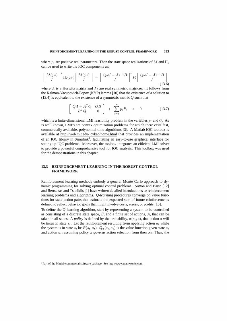
REINFORCEMENT LEARNING IN THE ROBUST CONTROL FRAMEWORK 333
wherepi are positive real parameters. Then the state space realizations ofM andΠi
can be used to write the IQC components as:∣∣∣∣
M(jω)I
∣∣∣∣∗Πi(jω)
∣∣∣∣M(jω)
I
∣∣∣∣ =∣∣∣∣
(jωI −A)−1BI
∣∣∣∣∗Pi
∣∣∣∣(jωI −A)−1B
I
∣∣∣∣(13.6)
whereA is a Hurwitz matrix andPi are real symmetric matrices. It follows fromthe Kalman-Yacubovich-Popov (KYP) lemma [10] that the existence of a solution to(13.4) is equivalent to the existence of a symmetric matrixQ such that
[QA + AT Q QB
BT Q 0
]+
n∑
i=1
piPi < 0 (13.7)
which is a finite-dimensional LMI feasibility problem in the variablespi andQ. Asis well known, LMI’s are convex optimization problems for which there exist fast,commercially available, polynomial time algorithms [3]. A Matlab IQC toolbox isavailable at http://web.mit.edu/˜cykao/home.htmlthat provides an implementationof an IQC library in Simulink1, facilitating an easy-to-use graphical interface forsetting up IQC problems. Moreover, the toolbox integrates an efficient LMI solverto provide a powerful comprehensive tool for IQC analysis. This toolbox was usedfor the demonstrations in this chapter.
13.3 REINFORCEMENT LEARNING IN THE ROBUST CONTROLFRAMEWORK
Reinforcement learning methods embody a general Monte Carlo approach to dy-namic programming for solving optimal control problems. Sutton and Barto [12]and Bertsekas and Tsitsiklis [1] have written detailed introductions to reinforcementlearning problems and algorithms.Q-learningprocedures converge on value func-tions for state-action pairs that estimate the expected sum of future reinforcementsdefined to reflect behavior goals that might involve costs, errors, or profits [13].
To define the Q-learning algorithm, start by representing a system to be controlledas consisting of a discrete state space,S, and a finite set of actions,A, that can betaken in all states. Apolicy is defined by the probability,π(st, a), that actiona willbe taken in statest. Let the reinforcement resulting from applying actionat whilethe system is in statest beR(st, at). Qπ(st, at) is the value function given statest
and actionat, assuming policyπ governs action selection from then on. Thus, the
1Part of the Matlab commercial software package. See http://www.mathworks.com.

334 ROBUST REINFORCEMENT LEARNING USING IQCS
desired value ofQπ(st, at) is
Qπ(st, at) = Eπ
T∑
k=0
γkR(st+k, at+k)
, (13.8)
whereγ is a discount factor between 0 and 1 that weights reinforcement receivedsooner more heavily than reinforcement received later.R is later defined to be afunction of the magnitude of the state tracking error, so actions are preferred withminimalQ values. From the above expression, a procedure for updating theQ valuescan be defined by deriving the following Monte Carlo version of value iteration:
∆Qπ(st, at) = αt
[R(st, at) + γ min
a′∈AQπ(st+1, a
′)−Qπ(st, at)]
.(13.9)
This is what has become known as theQ-learningalgorithm. Watkins [13] proves thatit does converge to the optimal value function, meaning that selecting the action,a,that minimizesQ(st, a) for any statest will result in the optimal sum of reinforcementover time. The proof of convergence assumes that the sequence of step sizesαt
satisfies the stochastic approximation conditions∑
αt = ∞ and∑
α2t < ∞. It also
assumes that every state and action are visited infinitely often and everyQ value isrepresented independently of all others.
TheQ function implicitly defines the policy,π, defined as
π(st) = argmina∈A
Q(st, a). (13.10)
However, asQ is being learned,π will certainly not be an optimal policy. A varietyof actions must be taken from every state in order to learn sufficiently accurateQvalues for the state-action pairs that are encountered. In the following experiment, arandom action was taken with probabilitypt for stept, wherept+1 = λpt, p0 = 1,and0 < λ < 1. Thus, the value ofpt approaches 0 with time and the policy slowlyshifts from a random policy to one determined by the learnedQ function.
Here Q-learning is combined with a fixed, robust controller by adding the actionchosen by the policy to the output of the fixed controller. The reinforcement learningobjective is to find a policy that minimizes the sum of the magnitude of the differencebetween a reference input and the system’s state variable that is meant to track thatreference input. To embed Q-learning in the robust control framework, the policymust be defined explicitly in a form that can be included in stability analysis. Todo so, an artificial neural network, called the actor network, is trained to duplicatethe Q-learning policy. This architecture is shown in Figure 13.2. The Q function islearned by the critic component that, in the following demonstrations, is implementedas a table.
TheQ function is not part of the feedback loop, so has no direct effect on the stabilityanalysis. However, the actor network is part of the feedback loop and is part ofthe stability analysis. The activation functions in the units of the actor network are
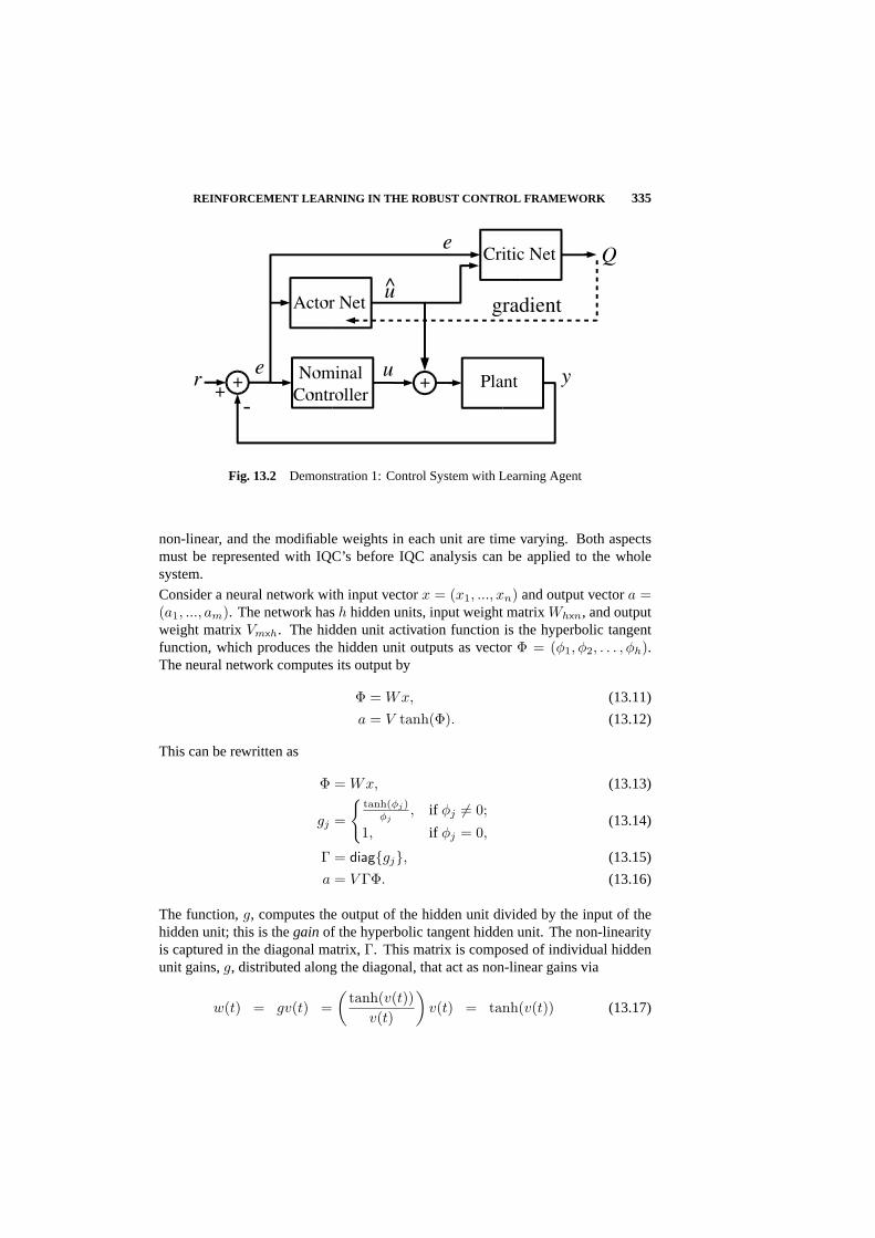
REINFORCEMENT LEARNING IN THE ROBUST CONTROL FRAMEWORK 335
Fig. 13.2 Demonstration 1: Control System with Learning Agent
non-linear, and the modifiable weights in each unit are time varying. Both aspectsmust be represented with IQC’s before IQC analysis can be applied to the wholesystem.
Consider a neural network with input vectorx = (x1, ..., xn) and output vectora =(a1, ..., am). The network hash hidden units, input weight matrixWhxn, and outputweight matrixVmxh. The hidden unit activation function is the hyperbolic tangentfunction, which produces the hidden unit outputs as vectorΦ = (φ1, φ2, . . . , φh).The neural network computes its output by
Φ = Wx, (13.11)
a = V tanh(Φ). (13.12)
This can be rewritten as
Φ = Wx, (13.13)
gj =
tanh(φj)
φj, if φj 6= 0;
1, if φj = 0,(13.14)
Γ = diaggj, (13.15)
a = V ΓΦ. (13.16)
The function,g, computes the output of the hidden unit divided by the input of thehidden unit; this is thegain of the hyperbolic tangent hidden unit. The non-linearityis captured in the diagonal matrix,Γ. This matrix is composed of individual hiddenunit gains,g, distributed along the diagonal, that act as non-linear gains via
w(t) = gv(t) =(
tanh(v(t))v(t)
)v(t) = tanh(v(t)) (13.17)
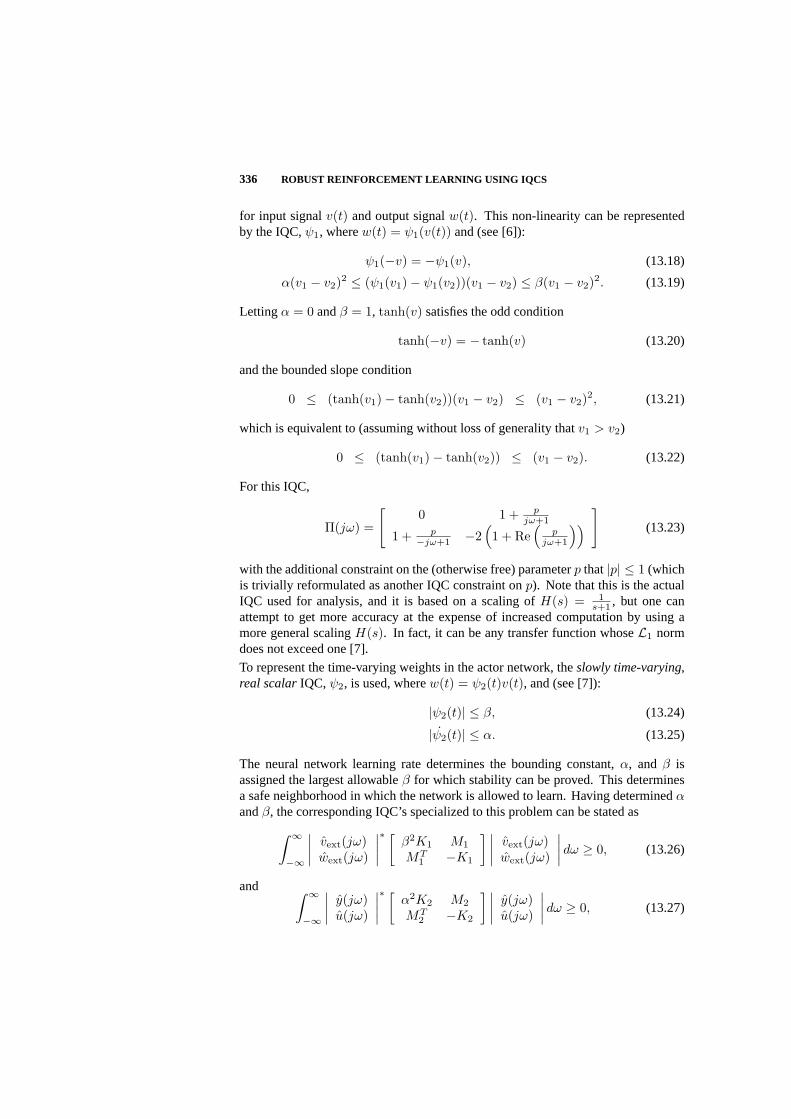
336 ROBUST REINFORCEMENT LEARNING USING IQCS
for input signalv(t) and output signalw(t). This non-linearity can be representedby the IQC,ψ1, wherew(t) = ψ1(v(t)) and (see [6]):
ψ1(−v) = −ψ1(v), (13.18)
α(v1 − v2)2 ≤ (ψ1(v1)− ψ1(v2))(v1 − v2) ≤ β(v1 − v2)2. (13.19)
Lettingα = 0 andβ = 1, tanh(v) satisfies the odd condition
tanh(−v) = − tanh(v) (13.20)
and the bounded slope condition
0 ≤ (tanh(v1)− tanh(v2))(v1 − v2) ≤ (v1 − v2)2, (13.21)
which is equivalent to (assuming without loss of generality thatv1 > v2)
0 ≤ (tanh(v1)− tanh(v2)) ≤ (v1 − v2). (13.22)
For this IQC,
Π(jω) =
[0 1 + p
jω+1
1 + p−jω+1 −2
(1 + Re
(p
jω+1
))]
(13.23)
with the additional constraint on the (otherwise free) parameterp that|p| ≤ 1 (whichis trivially reformulated as another IQC constraint onp). Note that this is the actualIQC used for analysis, and it is based on a scaling ofH(s) = 1
s+1 , but one canattempt to get more accuracy at the expense of increased computation by using amore general scalingH(s). In fact, it can be any transfer function whoseL1 normdoes not exceed one [7].
To represent the time-varying weights in the actor network, theslowly time-varying,real scalarIQC, ψ2, is used, wherew(t) = ψ2(t)v(t), and (see [7]):
|ψ2(t)| ≤ β, (13.24)
|ψ2(t)| ≤ α. (13.25)
The neural network learning rate determines the bounding constant,α, andβ isassigned the largest allowableβ for which stability can be proved. This determinesa safe neighborhood in which the network is allowed to learn. Having determinedαandβ, the corresponding IQC’s specialized to this problem can be stated as
∫ ∞
−∞
∣∣∣∣vext(jω)wext(jω)
∣∣∣∣∗ [
β2K1 M1
MT1 −K1
] ∣∣∣∣vext(jω)wext(jω)
∣∣∣∣ dω ≥ 0, (13.26)
and ∫ ∞
−∞
∣∣∣∣y(jω)u(jω)
∣∣∣∣∗ [
α2K2 M2
MT2 −K2
] ∣∣∣∣y(jω)u(jω)
∣∣∣∣ dω ≥ 0, (13.27)

REINFORCEMENT LEARNING IN THE ROBUST CONTROL FRAMEWORK 337
where the free parametersK1,K2,M1,M2 are subject to the additional (IQC) con-straints thatK1,K2 are symmetric positive definite matrices, andM1,M2 are skew-symmetric matrices. The signalsvext, wext are defined in terms ofv, w and anadditional (free) signalu as
vext(s) =[
v(s)s+1
v(s)
], wext(s) =
[w(s)s+1 + u(s)
s+1
w(s)
]. (13.28)
Note again that this is the actual IQC used for analysis, but in fact there are freescaling parameters in this IQC which are simply assigned as1
s+1 . A more generalstatement of this IQC (with more general scalings) can be found in [6].
The remainder of this section describes the algorithm for robust, reinforcementlearning control used for the demonstrations in the following section.
The input to the actor network is the error,et, between the reference input,rt, andthe actual state variable,yt, that must track the reference:
et = rt − yt. (13.29)
Givenet, the outputs of the hidden units,Φt, and the output unit,at, are
Φt = tanh(Wtet), (13.30)
at =
VtΦt, with probability1− εt;VtΦt + arand, with probabilityεt, wherearand is a Gaussian
random variable with mean 0 and variance 0.05.
(13.31)
Let the control law implemented by the robust, fixed controller bef . The outputsof the fixed controller and the actor network are summed and applied as the controlsignalut to the plant being controlled. Leth be the model of the plant that mapscontrol inputu to the next sampled value ofy.
ut = f(et) + at (13.32)
yt+1 = h(ut) (13.33)
Again calculate the error,et+1, and the hidden and output values of the neuralnetwork,Φt+1 andat+1.
et+1 = rt+1 − yt+1 (13.34)
Φt+1 = tanh(Wtet+1) (13.35)
at+1 =
VtΦt+1, with probability1− εt+1;VtΦt+1 + arand, with probabilityεt+1, wherearand is a Gaussian
random variable with mean 0 and variance 0.05
(13.36)

338 ROBUST REINFORCEMENT LEARNING USING IQCS
The reinforcement,Rt+1, isRt+1 = |et+1|. (13.37)
et andat are the inputs to theQ function table. LetQindex be a function that mapset
andat to the corresponding index into theQ table. To update the actor network, theoptimal action,a∗t , at stept is estimated by minimizing the value ofQ for n differentaction inputs,ai, in a local region of the action space centered onat, for which theestimate of the optimal action is given by
a∗t = argminai
QQindex(et,ai). (13.38)
Updates to the weights of the actor network are proportional to the difference betweenthis estimated optimal action and the actual action:
Vt+1 = Vt + β(a∗t − at)ΦTt , (13.39)
Wt+1 = Wt + βV T (a∗t − at) · (1− Φt · Φt)et, (13.40)
where· represents component-wise multiplication. TheQ value for stept is updatedby
QQindex(et,at) = QQindex(et,at) + α(Rt+1 + γQQindex(et+1,at+1) −QQindex(et,at)).(13.41)
Now it must be determined whether or not the new weight values,Wt+1 andVt+1,remain within the stable regionS. Initial values forW andV are random variablesfrom a Gaussian distribution with mean zero and variance of 0.1. The stable region,S, is always a rectangle in the multi-dimensional weight space and is initially centeredat zero. The size ofS is determined by an iterative expanding search described belowinvolving small increases to the size and a stability analysis until a maximum sizeis reached or stability cannot be guaranteed. If the new weight values fall withinS,S remains unchanged. Otherwise a new value forS is determined by the followingprocedure.
The actor network’s weight values are collected into one vector,C. An initial guessat allowed weight perturbations,P , as factors of the current weights is defined to beproportional to the current weight values:
C = (Wt, Vt) = (c1, c2, . . . ), (13.42)
P =C∑i ci
. (13.43)
These perturbation factors are adjusted to estimate the largest factors for which thesystem remains stable. Letzu andzs be scalar multipliers of the perturbation factorsfor which the system is not-guaranteed and guaranteed stable, respectively. They areinitialized tozu = zs = 1. The value ofzu is iteratively increased by2zu until thesystem with actor weightsC ± zuP ·C is not guaranteed stable. Similarly, the value

DEMONSTRATIONS OF ROBUST REINFORCEMENT LEARNING 339
of zs is iteratively decreased by12zs until the system with actor weightsC±zsP ·C isguaranteed stable. Now a finer search between is performed to decrease the intervalbetweenzs andzu :
Whilezu − zs
zs> 0.05 do (13.44)
zm =zu + zs
2(13.45)
If not stable forC ± zmP · C, setzu = zm, (13.46)
If stable forC ± zmP · C, setzs = zm. (13.47)
The resulting stable perturbations,zsP · C, now define the new set of stable weightregions,S = C ± zsP · C.
13.4 DEMONSTRATIONS OF ROBUST REINFORCEMENT LEARNING
13.4.1 First Demonstration: A First-Order Positioning Task
The first demonstration involves a simple non-mechanical positioning task. A singleinput called the reference signal,r moves on the interval[−1, 1] at random points intime. The plant output,y, must trackr as closely as possible. The plant is a firstorder system and thus has one internal state variablex. A control signalu is providedby the controller to positiony closer tor. The dynamics of the discrete-time systemare given by:
x(k + 1) = x(k) + u(k) (13.48)
y(k) = x(k) (13.49)
wherek is the discrete time step representing0.01 seconds of elapsed time. A simpleproportional controller (the control output is proportional to the size of the currenterror) is implemented withKp = 0.1:
e(k) = r(k)− y(k); (13.50)
u(k) = Kpe(k). (13.51)
For this demonstration, the critic is implemented using a lookup-table with inputseandu and output,Q(e, u). Each input is quantized into 25 intervals forming a 25x25matrix. The actor network is a two-layer, feed-forward neural network with a singleinput,e. There are threetanh hidden units, and one output unit providing actiona.Each unit includes a bias weight. The outputa is added to the output of the feedbackcontroller. This arrangement is depicted in block diagram form in Figure 13.2.
For training, the reference inputr is changed to a new value on the interval[−1, 1]stochastically with an average period of 20 time steps (every half second of simulatedtime). Training proceeded for 2000 time steps at learning rates ofα = 0.5 and

340 ROBUST REINFORCEMENT LEARNING USING IQCS
Fig. 13.3 Demonstration 1: Nominal System
Fig. 13.4 Demonstration 1: With Neuro-Controller
β = 0.1 for the critic and actor networks, respectively, then for an additional 2000time steps with learning rates ofα = 0.1 andβ = 0.01.
Figure 13.3 depicts a Simulink diagram for the nominal control system. This isreferred to as the nominal system because there is no learning component addedto the system. The plant is represented by a rectangular block that implements adiscrete-time state space system. The simple proportional controller is implementedby a triangular gain block. Another gain block provides the negative feedbackpath. The reference input is drawn from the left and the system output exits to theright. Figure 13.4 shows the addition of a actor network in parallel to the nominalcontroller. The combination of a nominal controller and the actor network will bereferred to as a neuro-controller. This diagram is suitable for conducting simulationstudies in Simulink. However, this diagram cannot be used for stability analysis,because the neural network is not represented as an LTI system. For static stabilityanalysis, assume constant gain matrices for the hidden layer weights,W , and theoutput layer weights,V . The static stability test will verify whether this particularneuro-controller implements a stable control system. Since the critic is not used inthe stability analysis, it is not included in this Simulink diagram.
Figure 13.5 shows the LTI version of the same system. The non-lineartanh functionis replaced by the single IQC block labeledodd slope non-linearityfrom the IQC-βMatlab toolbox by Megretski, et al., [6]. Theperformanceblock is another IQCblock that must be included in all IQC Simulink diagrams.

DEMONSTRATIONS OF ROBUST REINFORCEMENT LEARNING 341
Fig. 13.5 Demonstration 1: With Neuro-Controller as LTI (IQC)
There are actuallytwo versions of the neuro-controller. In the first version, shownin Figure 13.4, the actor network includes its non-linearities. This is the actualactor network that will be used as a controller in the system. The second versionof the system, shown in Figure 13.5, contains the actor network converted into theLTI framework; the non-lineartanh hidden layer has been replaced with an LTIuncertainty. This version of the neural network will never be implemented as acontroller; the sole purpose of this version is to analyze stability. Because the LTIsystemover-estimatesthe gain of the non-linearity in the non-LTI system, a stabilityguarantee on the LTI version implies a stability guarantee on the non-LTI system.
The IQC analysis procedure performs a feasibility search for a matrix satisfyingthe IQC inequality. If the search is feasible, the system is guaranteed stable; if thesearch is infeasible, the system is not guaranteed to be stable. When applied to theSimulink diagram, the feasibility constraints are easily satisfied; the neuro-controlleris guaranteed to be stable.
Additional constraints are now imposed on the learning algorithm in order to ensurethe network is dynamically stable while learning. The constraints are in the formof bounds on the perturbations,dW anddV , allowed on the actor network’s weightvalues, as shown in Figure 13.5. The rate by which the weight values are allowed tochange is also bounded. This constraint is implemented using theslowly time-varyingIQC block as shown in Figure 13.6.
The matricesWA, WB, V A, andV B re-dimension the sizes ofW andV ; theyhave no affect on the uncertainty or norm calculations. In the diagram,dW anddV contain all the individual perturbations along the diagonal whileW andV arenot diagonal matrices. Thus,Whxn anddWhnxhn are not dimensionally compatible.By multiplying with WA andWB this dimensional incompatibility is fixed withoutaffecting any of the numeric computations. Similarly,V A andV B are applied toVanddV .
The stability phase algorithm interacts with the Simulink diagram in Figure 13.6 tofind the largest set of uncertainties (the largest perturbations) for which the system isstill stable. Furthermore, the system will remain stable if the actor network weightvalues are changed as long as the new weight values do not exceed the range specified

342 ROBUST REINFORCEMENT LEARNING USING IQCS
Fig. 13.6 Demonstration 1: Simulink Diagram for Dynamic IQC-analysis
by the perturbation matrices,dW anddV . In the learning phase, the reinforcementlearning algorithm is applied until one of the network’s weight values exceeds therange specified by the perturbations.
The results of applying the above robust, reinforcement learning controller to the firsttask are now described. Observations follow on the trajectory of the actor weights inthe context of robust constraints.
The system is tested for a 10 second period (1000 discrete time steps with a sam-pling period of 0.01). The tracking performance of the trained system is shown inFigure 13.4. The top diagram shows the system performance with just the nominalcontroller, and the bottom graph shows performance with the trained neuro-controller.
The sum of the squared tracking error (SSE) is calculated over the 10 second interval.For the proportional only controller, theSSE = 33.20. Adding the neuro-controllerreduced theSSE to 11.73. The reinforcement learning neuro-controller is able toimprove the tracking performance. However, with this simple first-order system it isnot difficult to construct a better performing proportional controller. In fact, settingthe constant of proportionality to 1 (Kp = 1) achieves optimal control (minimalcontrol error). A suboptimal controller is purposely chosen in this demonstrationso that the neuro-controller has room to learn to improve control performance. Theeffect is similar to what would result if the value of a parameter of the plant was notaccurately known, in which case the controller would not be as aggressive as it couldbe. Kp would have to be less than 1.
In order to understand the operation of the constrained reinforcement learning agent,a minimal actor net with a single hidden unit is used so that the results can besummarized in a two-dimensional plot. The actor network has two inputs (the bias =1 and the tracking errore), onetanh hidden unit, and one output (u). Thus, there areonly two weights in this net with variable inputs. This network is still able to learn arelatively good control function, though three hidden units resulted in faster learning.
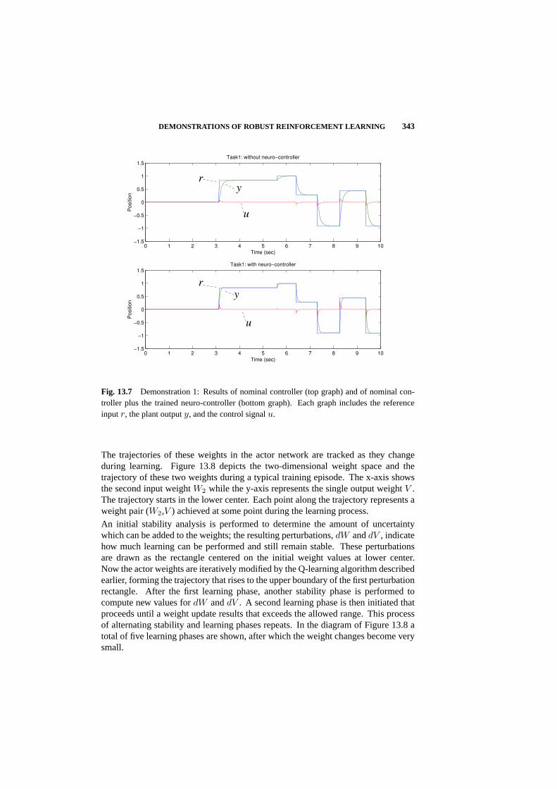
DEMONSTRATIONS OF ROBUST REINFORCEMENT LEARNING 343
0 1 2 3 4 5 6 7 8 9 10−1.5
−1
−0.5
0
0.5
1
1.5Task1: without neuro−controller
Time (sec)
Positio
n
0 1 2 3 4 5 6 7 8 9 10−1.5
−1
−0.5
0
0.5
1
1.5Task1: with neuro−controller
Positio
n
Time (sec)
r
y
u
y
u
r
Fig. 13.7 Demonstration 1: Results of nominal controller (top graph) and of nominal con-troller plus the trained neuro-controller (bottom graph). Each graph includes the referenceinputr, the plant outputy, and the control signalu.
The trajectories of these weights in the actor network are tracked as they changeduring learning. Figure 13.8 depicts the two-dimensional weight space and thetrajectory of these two weights during a typical training episode. The x-axis showsthe second input weightW2 while the y-axis represents the single output weightV .The trajectory starts in the lower center. Each point along the trajectory represents aweight pair (W2,V ) achieved at some point during the learning process.
An initial stability analysis is performed to determine the amount of uncertaintywhich can be added to the weights; the resulting perturbations,dW anddV , indicatehow much learning can be performed and still remain stable. These perturbationsare drawn as the rectangle centered on the initial weight values at lower center.Now the actor weights are iteratively modified by the Q-learning algorithm describedearlier, forming the trajectory that rises to the upper boundary of the first perturbationrectangle. After the first learning phase, another stability phase is performed tocompute new values fordW anddV . A second learning phase is then initiated thatproceeds until a weight update results that exceeds the allowed range. This processof alternating stability and learning phases repeats. In the diagram of Figure 13.8 atotal of five learning phases are shown, after which the weight changes become verysmall.

344 ROBUST REINFORCEMENT LEARNING USING IQCS
Fig. 13.8 Demonstraton 1: Trajectory of values of weights in the actor network whilelearning. Superimposed are the bounding boxes of regions for which weight values result instable behavior.
It is important to note that if the trajectory reaches the edge of a bounding box, theweights may still be able to be adjusted in that direction. Recall that the edges of thebounding box are computedwith respect to the network weight values at the time ofthe stability phase; these initial weight values are the point along the trajectory in theexact center of the bounding box. This central point in the weight space is the value ofthe actor network weights at the beginning of this particular stability/learning phase.Given that the current network weight values are that central point, the boundingbox is thelimit of weight changes that the network tolerates without forfeiting thestability guarantee. This is not to be confused with anabsolutelimit on the size ofthat network weight.
The third phase of the trajectory reveals some interesting dynamics. The trajectorystops near the edge of the box, and moves back toward the middle. Keep in mind thatthis trajectory represents the weight changes in the actor network. At the same timeas the actor network is learning, the critic is also learning and adjusting its weights.During this phase in the training, the critic’s predictions become more accurate.Because the gradient of the critic directs the weight changes for the actor network,the direction of weight changes in the actor network reverses. In the early part of thelearning the critic network gradient indicates that “upper left” is a desirable trajectoryfor weight changes in the actor network. By the third phase, the critic has changed to

DEMONSTRATIONS OF ROBUST REINFORCEMENT LEARNING 345
0 -0.5 -1.00.51.0
yr
Mass
Friction
Spring
Fig. 13.9 Demonstration 2: Mass, Spring, Dampening System
indicate that “upper-left” is now an undesirable direction for movement for the actornetwork.
Further dynamics are revealed in the last two phases. The actor network weights arenot changing as rapidly as they did in the earlier learning phases. Optimal trackingperformance according to the gradient in the critic is being achieved. The point ofconvergence of the actor network weights is a local optima in the value function ofthe critic. Training is halted at this point because the actor weights have ceased tochange.
13.4.2 Second Demonstration: A Second-Order System
The second demonstration involves a second order mass/spring/dampener system,providing a more challenging and more realistic system in which to test the robust,reinforcement-learning algorithm. Once again, a single reference inputr movesstochastically on the interval[−1, 1]; the single output of the control systemy musttrackr as closely as possible. However, there are now friction, inertial, and springforces acting on the system. Figure 13.9 depicts the different components of thesystem. The discrete-time update equations are given by
e(k) = r(k)− y(k), (13.52)
u(k) = Kpe(k) +∫
Kie(k), (13.53)
Kp = 0.01 Ki = 0.001, (13.54)
x(k + 1) =[
1 0.05−0.05 0.9
]x(k) +
[0
1.0
]u(k), (13.55)
y(k) =[
1 0]x(k). (13.56)
Here, the nominal controller is a PI controller with both aproportional term and anintegral term. This controller is implemented with its own internal state variable.The more advanced controller is required in order to provide reasonable nominal

346 ROBUST REINFORCEMENT LEARNING USING IQCS
control for a system with second-order dynamics. The constant of proportionality,Kp, is 0.01, and the integral constant,Ki, is 0.001. Once again, a controller withsuboptimal performance is chosen so that the RL agent has significant margin forimprovement.
The architecture of the learning components is almost identical to that used in thefirst demonstration. The actor network consists of two inputs (the bias term and thecurrent tracking error), three hidden units, and one output (the addition to the controlsignal).
The reference inputr is changed to a new value on the interval[−1, 1] stochasticallywith an average period of 20 time steps (every half second of simulated time). Dueto the more difficult second-order dynamics, the training time is increased to 10,000time steps at learning rates ofα = 0.5 andβ = 0.1 for the critic and actor networksrespectively. Then an additional 10,000 steps of training are taken with learning ratesof α = 0.1 andβ = 0.01.
Figure 13.10 shows the results of testing a trained system. The top portion ofthe diagram depicts the nominal control system (with only the PI controller) whilethe bottom half shows the same system with both the PI controller and the neuro-controller acting together. Recall thatKi andKp parameters aresuboptimalso thatthe neural network has opportunity to improve the control system. The addition ofthe neuro-controller clearly does improve system tracking performance. The totalsquared tracking error for the nominal system isSSE = 246.6 while the total squaredtracking error for the neuro-controller isSSE = 76.3.
To demonstrate the advantage provided by stability analysis, two training scenariosare analyzed. The first training scenario involved the stable reinforcement learn-ing algorithm with IQC-analysis. In the second training scenario, training proceedswithout the constraints imposed by the stability analysis. Both scenarios result insimilar control performance; all produce similar weights for the actor network. Whileboth scenarios result in a stable controller as an end product (the final neural networkweight values), only the scenario trained with IQC constraints enforced retains stabil-ity throughoutthe training. The stand-alone reinforcement learning scenario actuallyproduces unstable intermediate neuro-controllers during the learning process.
An example of this behavior is shown in Figure 13.11. Clearly, the actor net is notimplementing a good control solution; the system has been placed into an unstablelimit cycle, because of the actor network. Notice the scale of the y-axis compared tothe stable control diagram of Figure 13.10. This is exactly the type of scenario thatmust be avoided if neuro-controllers are to be useful in industrial control applications.To verify the instability of this system, these temporary actor network weights areused for a static stability test. IQC-analysis is unable to find a feasible solution,indicating that the system is indeed unstable.
In summary, the purpose of this demonstration is to construct a control system withdynamics adequately simple to be amenable to introspection, but also adequatelycomplex to introduce the possibility of learning/implementing unstable controllers.In this task the restrictions imposed on weights from the dynamic stability analysisare necessary to keep the neuro-control system stable during reinforcement learning.
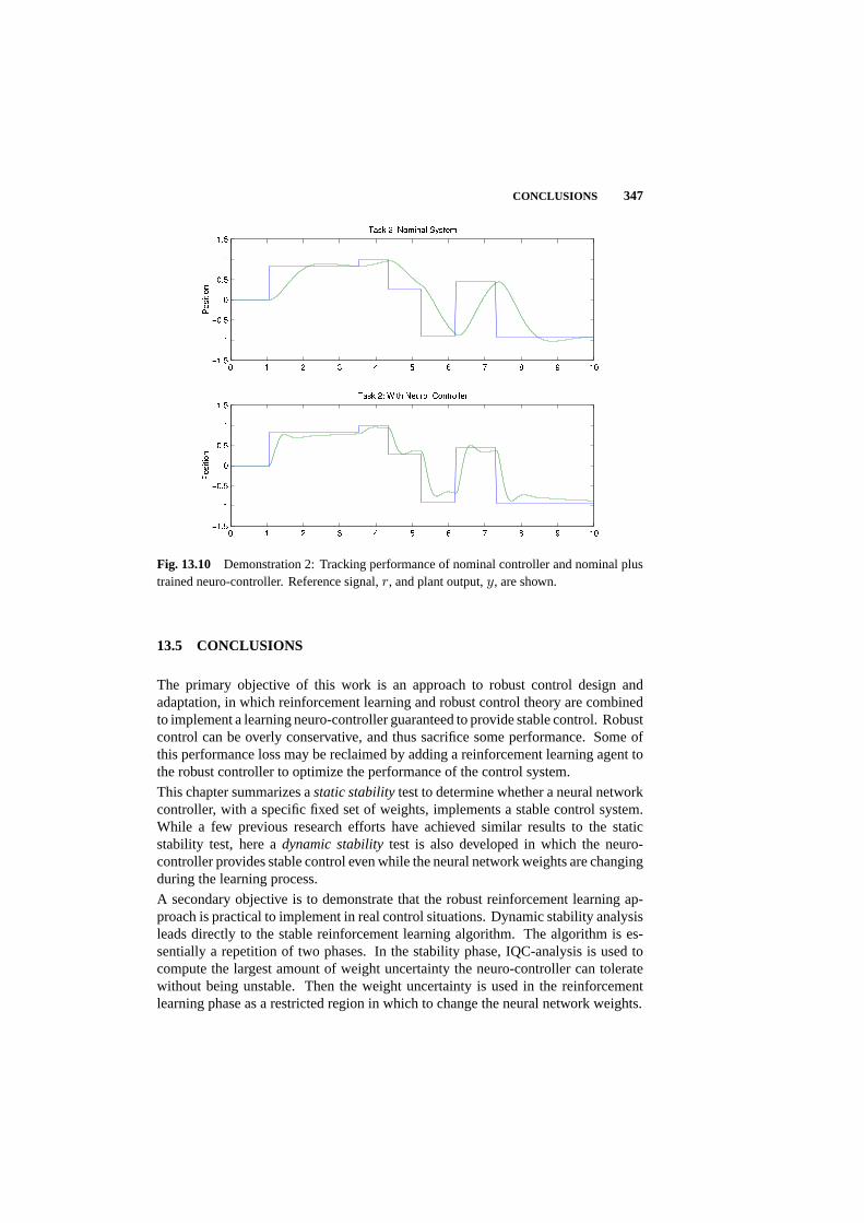
CONCLUSIONS 347
Fig. 13.10 Demonstration 2: Tracking performance of nominal controller and nominal plustrained neuro-controller. Reference signal,r, and plant output,y, are shown.
13.5 CONCLUSIONS
The primary objective of this work is an approach to robust control design andadaptation, in which reinforcement learning and robust control theory are combinedto implement a learning neuro-controller guaranteed to provide stable control. Robustcontrol can be overly conservative, and thus sacrifice some performance. Some ofthis performance loss may be reclaimed by adding a reinforcement learning agent tothe robust controller to optimize the performance of the control system.
This chapter summarizes astatic stabilitytest to determine whether a neural networkcontroller, with a specific fixed set of weights, implements a stable control system.While a few previous research efforts have achieved similar results to the staticstability test, here adynamic stabilitytest is also developed in which the neuro-controller provides stable control even while the neural network weights are changingduring the learning process.
A secondary objective is to demonstrate that the robust reinforcement learning ap-proach is practical to implement in real control situations. Dynamic stability analysisleads directly to the stable reinforcement learning algorithm. The algorithm is es-sentially a repetition of two phases. In the stability phase, IQC-analysis is used tocompute the largest amount of weight uncertainty the neuro-controller can toleratewithout being unstable. Then the weight uncertainty is used in the reinforcementlearning phase as a restricted region in which to change the neural network weights.

348 ROBUST REINFORCEMENT LEARNING USING IQCS
Fig. 13.11 Demonstration 2: System becomes unstable at an intermediate stage while learn-ing. Two state variables, the control signal,u, and the reference signal,r, are shown.
This approach to robust reinforcement learning remains to be tested on realisticcontrol tasks more difficult than the simple demonstrations described in this chapter.In real applications, one problem may be the training time on the physical systemwhich could be prohibitively expensive as the system must be driven through all ofits dynamics multiple times. The advantage of this approach is limited in situationswhere the physical plant and plant model closely match each other or cases in whichdifferences between the model and plant do not greatly affect the dynamics.
In current work the robust reinforcement learning procedure is being extended to moredifficult control problems (Chapter 20). Additional ways of capitalizing on the theoryof static and dynamic stability using IQC’s are being developed for other categoriesof action function approximators and for including robust stability objectives in thereinforcement function.
Acknowledgments
This work was supported by the National Science Foundation through grants CMS-9401249and CISE-9422007.

Bibliography
1. D. P. Bertsekas and J. N. Tsitsiklis,Neuro-Dynamic Programming,Athena Scien-tific, Belmont, MA, 1995.
2. John C. Doyle, Bruce A. Francis, and Allen R. Tannenbaum,Feedback ControlTheory,Macmillan Publishing Company, 1992.
3. Pascal Gahihet, Arkadi Nemirovski, Alan J. Laub, and Mahmoud Chilali,LMIControl Toolbox,MathWorks Inc., 1995.
4. R. Matthew Kretchmar,A Synthesis of Reinforcement Learning and Robust Con-trol Theory, PhD thesis, Colorado State University, Department of ComputerScience, 2000.
5. R.M. Kretchmar, P.M. Young, C.W. Anderson, D. Hittle, M. Anderson, C. Del-nero, and J. Tu, “Robust reinforcement learning control with static and dynamicstability,” International Journal of Robust and Nonlinear Control, 11:1469–1500,2001.
6. Alexandre Megretski, Chung-Yao KAO, Ulf Jonsson, and Anders Rantzer,AGuide to IQCβ: Software for Robustness Analysis,MIT / Lund Institute ofTechnology, http://www.mit.edu/people/ameg/home.html, 1999.
7. Alexandre Megretski and Anders Rantzer, “System analysis via integral quadraticconstraints,”IEEE Transactions on Automatic Control, 42(6):819–830, June 1997.
8. Alexandre Megretski and Anders Rantzer, “System analysis via integral quadraticconstraints: Part II,” Technical Report ISRN LUTFD2/TFRT–7559–SE, LundInstitute of Technology, September 1997.
9. A. Packard and J. Doyle, “The complex structured singular value,”Automatica,29(1):71–109, 1993.
10. Anders Rantzer, “On the Kalman-Yacubovich-Popov lemma,”Systems & Con-trol Letters, 28:7–10, 1996.
11. “Sigurd Skogestad and Ian Postlethwaite,”Multivariable Feedback Control,JohnWiley and Sons, 1996.
349

350 BIBLIOGRAPHY
12. Richard S. Sutton and Andrew G. Barto,Reinforcement Learning: An Introduc-tion, The MIT Press, 1998.
13. C.J.C.H. Watkins,Learning with Delayed Rewards,PhD thesis, CambridgeUniversity Psychology Department, Cambridge, England, 1989.
14. Kemin Zhou and John C. Doyle,Essentials of Robust Control,Prentice Hall,1998.
14 Supervised Actor-CriticReinforcement Learning
MICHAEL T. ROSENSTEIN and ANDREW G. BARTO
University of Massachusetts
Editor’s Summary: Chapter 7 introduced policy gradients as a way to improve onstochastic search of the policy space when learning. This chapter presents supervisedactor-critic reinforcement learning as another method for improving the effectivenessof learning. With this approach, a supervisor adds structure to a learning problemand supervised learning makes that structure part of an actor-critic framework forreinforcement learning. Theoretical background and a detailed algorithm descriptionare provided, along with several examples that contain enough detail to make themeasy to understand and possible to duplicate. These examples also illustrate the useof two kinds of supervisors: a feedback controller that is easily designed yet sub-optimal, and a human operator providing intermittent control of a simulated roboticarm.
14.1 INTRODUCTION
Reinforcement learning (RL) and supervised learning are usually portrayed as distinctmethods of learning from experience. RL methods are often applied to problemsinvolving sequential dynamics and optimization of a scalar performance objective,with online exploration of the effects of actions. Supervised learning methods, on theother hand, are frequently used for problems involving static input-output mappingsand minimization of a vector error signal, with no explicit dependence on how trainingexamples are gathered. As discussed by Barto and Dietterich (this volume), the keyfeature distinguishing RL and supervised learning is whether training informationfrom the environment serves as an evaluation signal or as an error signal, and in thischapter, we are interested in problems where both kinds of feedback are available toa learning systemat the same time.
As an example, consider a young child learning to throw a ball. For this motortask, as well as many others, there is no substitute for ongoing practice. The child
351
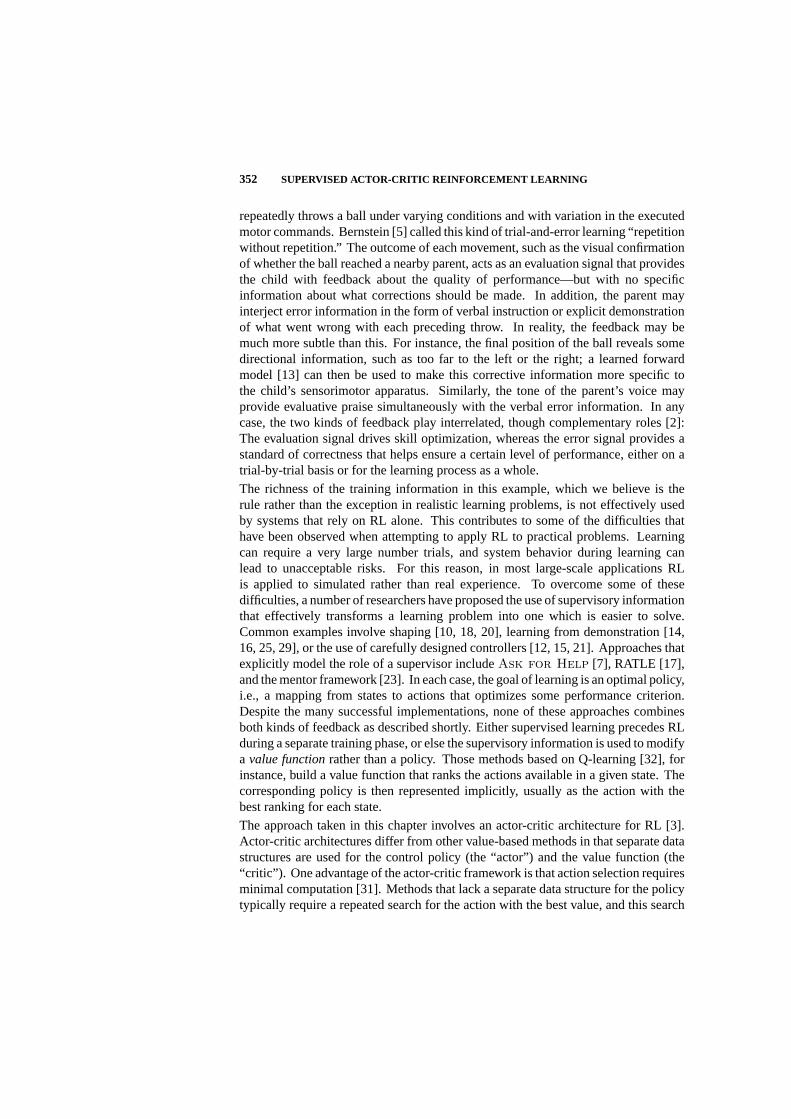
352 SUPERVISED ACTOR-CRITIC REINFORCEMENT LEARNING
repeatedly throws a ball under varying conditions and with variation in the executedmotor commands. Bernstein [5] called this kind of trial-and-error learning “repetitionwithout repetition.” The outcome of each movement, such as the visual confirmationof whether the ball reached a nearby parent, acts as an evaluation signal that providesthe child with feedback about the quality of performance—but with no specificinformation about what corrections should be made. In addition, the parent mayinterject error information in the form of verbal instruction or explicit demonstrationof what went wrong with each preceding throw. In reality, the feedback may bemuch more subtle than this. For instance, the final position of the ball reveals somedirectional information, such as too far to the left or the right; a learned forwardmodel [13] can then be used to make this corrective information more specific tothe child’s sensorimotor apparatus. Similarly, the tone of the parent’s voice mayprovide evaluative praise simultaneously with the verbal error information. In anycase, the two kinds of feedback play interrelated, though complementary roles [2]:The evaluation signal drives skill optimization, whereas the error signal provides astandard of correctness that helps ensure a certain level of performance, either on atrial-by-trial basis or for the learning process as a whole.
The richness of the training information in this example, which we believe is therule rather than the exception in realistic learning problems, is not effectively usedby systems that rely on RL alone. This contributes to some of the difficulties thathave been observed when attempting to apply RL to practical problems. Learningcan require a very large number trials, and system behavior during learning canlead to unacceptable risks. For this reason, in most large-scale applications RLis applied to simulated rather than real experience. To overcome some of thesedifficulties, a number of researchers have proposed the use of supervisory informationthat effectively transforms a learning problem into one which is easier to solve.Common examples involve shaping [10, 18, 20], learning from demonstration [14,16, 25, 29], or the use of carefully designed controllers [12, 15, 21]. Approaches thatexplicitly model the role of a supervisor includeAsk for Help [7], RATLE [17],and the mentor framework [23]. In each case, the goal of learning is an optimal policy,i.e., a mapping from states to actions that optimizes some performance criterion.Despite the many successful implementations, none of these approaches combinesboth kinds of feedback as described shortly. Either supervised learning precedes RLduring a separate training phase, or else the supervisory information is used to modifya value functionrather than a policy. Those methods based on Q-learning [32], forinstance, build a value function that ranks the actions available in a given state. Thecorresponding policy is then represented implicitly, usually as the action with thebest ranking for each state.
The approach taken in this chapter involves an actor-critic architecture for RL [3].Actor-critic architectures differ from other value-based methods in that separate datastructures are used for the control policy (the “actor”) and the value function (the“critic”). One advantage of the actor-critic framework is that action selection requiresminimal computation [31]. Methods that lack a separate data structure for the policytypically require a repeated search for the action with the best value, and this search
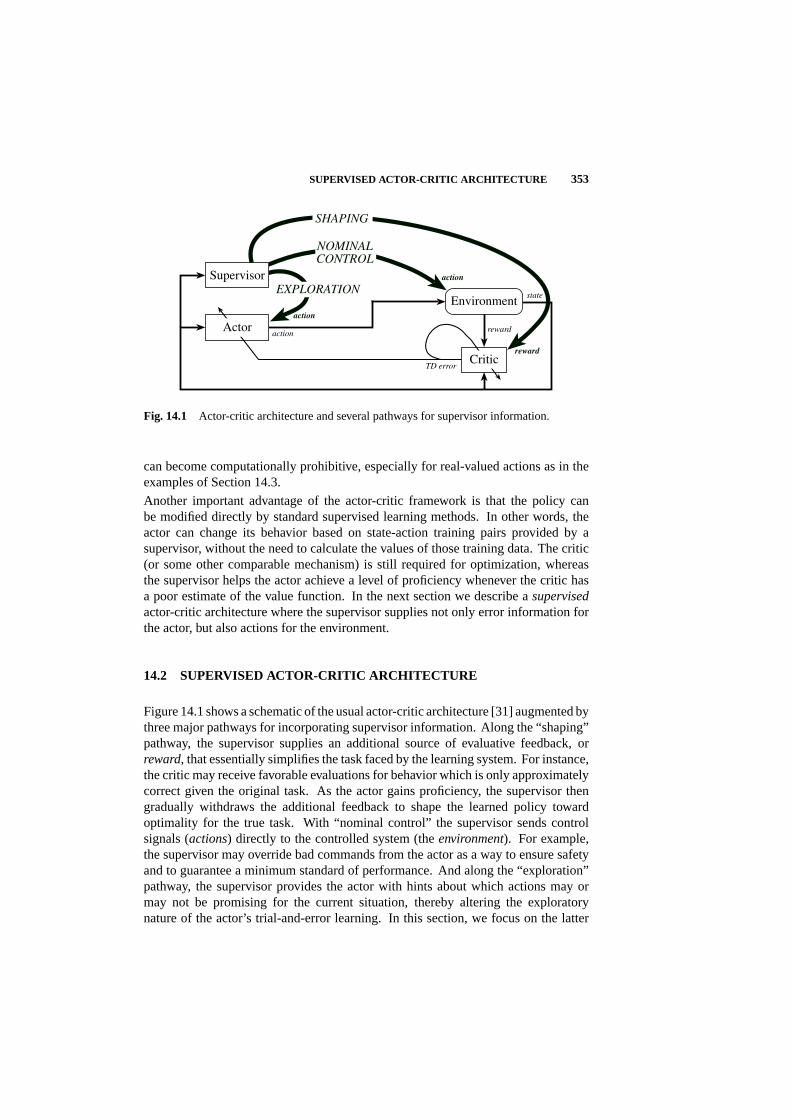
SUPERVISED ACTOR-CRITIC ARCHITECTURE 353
state
reward
TD error
action
Supervisor
Environment
Critic
Actor
SHAPING
EXPLORATION
NOMINAL
CONTROL
reward
action
action
Fig. 14.1 Actor-critic architecture and several pathways for supervisor information.
can become computationally prohibitive, especially for real-valued actions as in theexamples of Section 14.3.
Another important advantage of the actor-critic framework is that the policy canbe modified directly by standard supervised learning methods. In other words, theactor can change its behavior based on state-action training pairs provided by asupervisor, without the need to calculate the values of those training data. The critic(or some other comparable mechanism) is still required for optimization, whereasthe supervisor helps the actor achieve a level of proficiency whenever the critic hasa poor estimate of the value function. In the next section we describe asupervisedactor-critic architecture where the supervisor supplies not only error information forthe actor, but also actions for the environment.
14.2 SUPERVISED ACTOR-CRITIC ARCHITECTURE
Figure 14.1 shows a schematic of the usual actor-critic architecture [31] augmented bythree major pathways for incorporating supervisor information. Along the “shaping”pathway, the supervisor supplies an additional source of evaluative feedback, orreward, that essentially simplifies the task faced by the learning system. For instance,the critic may receive favorable evaluations for behavior which is only approximatelycorrect given the original task. As the actor gains proficiency, the supervisor thengradually withdraws the additional feedback to shape the learned policy towardoptimality for the true task. With “nominal control” the supervisor sends controlsignals (actions) directly to the controlled system (theenvironment). For example,the supervisor may override bad commands from the actor as a way to ensure safetyand to guarantee a minimum standard of performance. And along the “exploration”pathway, the supervisor provides the actor with hints about which actions may ormay not be promising for the current situation, thereby altering the exploratorynature of the actor’s trial-and-error learning. In this section, we focus on the latter

354 SUPERVISED ACTOR-CRITIC REINFORCEMENT LEARNING
statecomposite
action
reward
TD error
action
action
supervisory error
+
−
Supervisor
Environment
Critic
GainScheduler
Composite Actor
ΣActor
Fig. 14.2 The supervised actor-critic architecture.
two pathways, and we examine the use of supervised learning which offers a powerfulcounterpart to RL methods.
The combination of supervised learning with actor-critic RL was first suggested byClouse and Utgoff [8] and independently by Benbrahim and Franklin [4]. Theirapproach has received almost no attention, yet the more general problem of how tocombine a teacher with RL methods has become quite popular. In their work, Ben-brahim and Franklin [4] used pre-trained controllers, called “guardians,” to providesafety and performance constraints for a biped robot. Joint position commands weresent to the robot by a central pattern generator, but those commands were modifiedby the guardians whenever a constraint was violated. Superimposed with the jointposition commands were exploratory actions generated according to Gullapalli’sSRV algorithm [11]. In effect, the central pattern generator learned not only fromexploration, but from the guardians as well.
Figure 14.2 shows our version of the supervised actor-critic architecture, which differsfrom previous work in a key way described in Section 14.2.2. Taken together, theactor, the supervisor and the gain scheduler1 form a “composite” actor that sends acomposite action to the environment. The environment responds to this action witha transition from the current state,s, to the next state,s′. (Appendix 1 contains a listof symbols used throughout the remainder of this chapter.) The environment alsoprovides an evaluation called the immediate reward,r. The job of the critic is toobserve states and rewards and to build a value function,Vπ(s), that accounts forboth immediate and future rewards received under the composite policy,π. Thisvalue function is defined recursively as
Vπ(s) =∑
s′∈SPr(s′|s,a)R(s′) + γVπ(s′),
1“Gain scheduling” refers to the construction of a global nonlinear controller by interpolation, or schedul-ing, of local linear controllers [27]. We use the term in a broader sense to mean the blending of two ormore sources of control actions.

SUPERVISED ACTOR-CRITIC ARCHITECTURE 355
whereR(s′) is the expected value ofr, γ ∈ [0, 1] is a factor that discounts thevalue of the next state, and Pr(s′|s,a) is the probability of transitioning to states′
after executing actiona = π(s). Here we focus on deterministic policies, althoughthis work also generalizes to the stochastic case whereπ represents a distributionfor choosing actions probabilistically. For RL problems, the expected rewards andthe state-transition probabilities are typically unknown. Learning, therefore, mustproceed from samples, i.e., from observed rewards and state transitions. For RLalgorithms, temporal-difference (TD) methods [30] are commonly used to update thestate-valueestimates, V(s), by an amount proportional to the TD error, defined as
δ = r + γV(s′)− V(s).
14.2.1 The Gain Scheduler
For deterministic policies and real-valued actions, the gain scheduler computes thecomposite action,a, as simply a weighted sum of the actions given by the componentpolicies. In particular,
a← kaE + (1− k)aS,
whereaE is the actor’s exploratory action andaS is the supervisor’s action, as givenby policiesπE andπS, respectively. (The supervisor’s actions are observable but itspolicy is unknown.) We also denote byaA the actor’s greedy action determined bythe corresponding policy,πA. Typically, πE is a copy ofπA modified to include anadditive random variable with zero mean. Thus, each exploratory action is simply anoisy copy of the corresponding greedy action, although we allow for the possibilityof more sophisticated exploration strategies.
The parameterk ∈ [0, 1] interpolates betweenπE andπS, and thereforek determinesthe level of control, or autonomy, on the part of the actor.2 In general, the valueof k varies with state, although we drop the explicit dependence ons to simplifynotation. The parameterk also plays an important role in modifying the actor’spolicy, as described in more detail below. We assume thatπA is given by a functionapproximator with the parameter vectorw, and after each state transition, thoseparameters are updated according to a rule of the form
w← w + k∆wRL + (1− k)∆wSL, (14.1)
where∆wRL and ∆wSL are the individual updates based on RL and supervisedlearning, respectively. Thus,k also interpolates between two styles of learning.
The use ofk—a single state-dependent parameter that trades off between two sourcesof action and learning—allows for a wide range of interactions between actor andsupervisor. If the actor has control of the gain scheduler, for instance, then the actorcan set the value ofk near 0 whenever it needs help from its supervisor, cf.Ask
2For the stochastic case,k gives the probability that the gain scheduler chooses the actor’s exploratoryaction rather than the supervisor’s action.

356 SUPERVISED ACTOR-CRITIC REINFORCEMENT LEARNING
for Help [7]. Similarly, if the supervisor has control of the gain scheduler, then thesupervisor can setk = 0 whenever it loses confidence in the autonomous behavior ofthe actor, cf. RATLE [17]. The gain scheduler may even be under control of a thirdparty. For example, a linear feedback controller can play the role of supervisor, andthen a human operator can adjust the value ofk as a way to switch between actor andsupervisor, perhaps at a longer time scale than that of the primitive actions.
14.2.2 The Actor Update Equation
To make the reinforcement-based adjustment to the parameters ofπA we compute
∆wRL ← αδ(aE − aA)∇wπA(s), (14.2)
whereα is a step-size parameter. Eq. (14.2) is similar to the update used by theREINFORCEclass of algorithms [33], although we utilize the gradient of the de-terministic policyπA rather than that of the stochastic exploration policyπE. Whenthe TD error is positive, this update will push the greedy policy evaluated ats closerto aE, i.e., closer to the exploratory action which led to a state with estimated valuebetter than expected. Similarly, whenδ < 0, the update will pushπA(s) away fromaE and in subsequent visits to states the corresponding exploratory policy will selectthis unfavorable action with reduced probability.
To compute the supervised learning update,∆wSL, we seek to minimize in eachobserved state the supervisory error
E =12[πS(s)− πA(s)]2.
Locally, this is accomplished by following a steepest descent heuristic, i.e., by makingan adjustment proportional to the negative gradient of the error with respect tow:
∆wSL ← −α∇wE(s).
Expanding the previous equation with the chain rule and substituting the observedactions gives the usual kind of gradient descent learning rule:
∆wSL ← α(aS− aA)∇wπA(s). (14.3)
Finally, by substituting Eqs. (14.2) and (14.3) into Eq. (14.1) we obtain the desiredactor update equation:
w← w + α[kδ(aE − aA) + (1− k)(aS− aA)]∇wπA(s). (14.4)
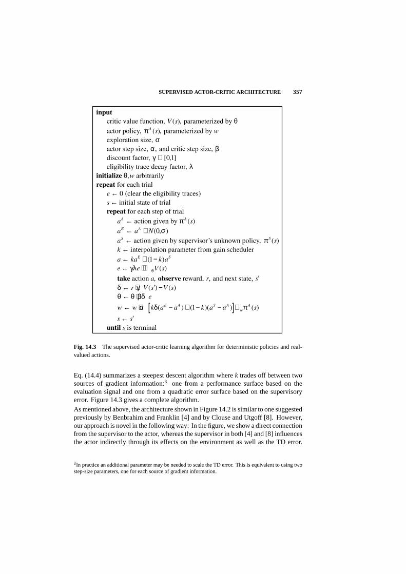
SUPERVISED ACTOR-CRITIC ARCHITECTURE 357
input
critic value function, V (s), parameterized by θactor policy, π A (s), parameterized by w
exploration size, σactor step size, α, and critic step size, βdiscount factor, γ ∈ [0,1]
eligibility trace decay factor, λinitialize θ,w arbitrarily
repeat for each trial
e ← 0 (clear the eligibility traces)
s ← initial state of trial
repeat for each step of trial
aA ← action given by π A (s)
aE ← a
A + N(0,σ )
aS ← action given by supervisor’s unknown policy, π S (s)
k ← interpolation parameter from gain scheduler
a ← kaE + (1− k)a
S
e ← γλe + ∇θV (s)
take action a, observe reward, r, and next state, ′sδ ← r + γV ( ′s ) −V (s)
θ ← θ + βδe
w ← w + α kδ(aE − aA ) + (1− k)(aS − a
A )[ ]∇wπ A (s)
s ← ′suntil s is terminal
Fig. 14.3 The supervised actor-critic learning algorithm for deterministic policies and real-valued actions.
Eq. (14.4) summarizes a steepest descent algorithm wherek trades off between twosources of gradient information:3 one from a performance surface based on theevaluation signal and one from a quadratic error surface based on the supervisoryerror. Figure 14.3 gives a complete algorithm.
As mentioned above, the architecture shown in Figure 14.2 is similar to one suggestedpreviously by Benbrahim and Franklin [4] and by Clouse and Utgoff [8]. However,our approach is novel in the following way: In the figure, we show a direct connectionfrom the supervisor to the actor, whereas the supervisor in both [4] and [8] influencesthe actor indirectly through its effects on the environment as well as the TD error.
3In practice an additional parameter may be needed to scale the TD error. This is equivalent to using twostep-size parameters, one for each source of gradient information.
358 SUPERVISED ACTOR-CRITIC REINFORCEMENT LEARNING
Using our notation the corresponding update equation for these other approaches,e.g., [4, Eq. (1)], essentially becomes
w← w + α[kδ(aE − aA) + (1− k)δ(aS− aA)]∇wπA(s) (14.5)
= w + αδ[kaE + (1− k)aS− aA]∇wπA(s). (14.6)
The key attribute of Eq. (14.5) is that the TD error modulates the supervisory error,aS− aA. This may be a desirable feature if one “trusts” the critic more than thesupervisor, in which case one should view the supervisor as an additional source ofexploration. However, Eq. (14.5) may cause the steepest descent algorithm to ascendthe associated error surface, especially early in the learning process when the critichas a poor estimate of the true value function. Moreover, whenδ is small, the actorloses the ability to learn from its supervisor, whereas in Eq. (14.4) this ability dependsprimarily on the interpolation parameter,k.
14.3 EXAMPLES
In this section we present several examples that illustrate a gradual shift from fullcontrol of the environment by the supervisor to autonomous control by the actor.In each case, the supervisor enables the composite actor in Figure 14.2 to solve thetaskon the very first trial, and on every trial while it improves, whereas the task isvirtually impossible to solve with RL alone. The first three examples are targetingtasks—each with a stable controller that brings the system to target, although in asub-optimal fashion. The final example involves a human supervisor that controls asimulated robot during a peg insertion task.
For each example we used the learning algorithm in Figure 14.3 with step-sizeparameters ofα = 0.1 for the actor andβ = 0.3 for the critic. To update the critic’svalue function, we used the TD(λ) algorithm [30] withλ = 0.7. We implementedboth actor and critic by a tile coding scheme, i.e., CMAC [1], with a total of 25 tilings,or layers, per CMAC. (Appendix 2 provides a brief description of CMAC functionapproximators.)
14.3.1 Ship Steering Task
For our first experiment we adapted a standard problem from the optimal controlliterature where the task is to steer a ship to a goal in minimum time [6]. Theship moves at a constant speed ofC = 0.01 km· s−1, and the real-valued stateand action are given, respectively, by the ship’s two-dimensional position and scalarheading. For this problem, the supervisor is a hand-crafted controller that alwayssteers directly toward the center of the goal region, i.e., toward the origin(0, 0). Underfull supervision, this strategy ensures that the ship will reach the goal eventually—but not in minimum time due to a water current that complicates the task. More

EXAMPLES 359
Goal
Start
y [
km
]
-2
-1
2
1
0 1 2
Optimal Path
WaterCurrentProfile
x [km]3 4 5 6
Fig. 14.4 Ship steering task simulator after 1000 learning trials. The grayscale regionindicates the level of autonomy, fromk = 0 (white) tok = 1 (black).
specifically, the equations of motion are
x = C (cosφ− y), y = C sinφ, (14.7)
whereφ is the ship’s heading. Notice that the water current acts along the horizontaldirection, x, yet depends solely on the vertical position,y. The start location isx0 = 3.66,y0 = −1.86, and the goal region has a of radius 0.1 km. A convenientfeature of this test problem is that one can solve for the optimal policy analytically [6],and the darker curve in Figure 14.4 shows the corresponding optimal path. Underthe optimal policy the minimum time to goal is 536.6 s while the supervisor’s timeto goal is 1111 s.
We integrated Eq. (14.7) numerically using Euler’s method with a step size of 1 s.Control decisions by the gain scheduler were made every 25 s, at which time the shipchanged heading instantaneously. Exploratory actions,aE, were Gaussian distributedwith a standard deviation of 10 degrees and a mean equal to the greedy action,aA.The CMAC tiles were uniform with a width of 0.5 km along each input dimension.The actor CMAC was initialized to steer the ship leftward while the critic CMACwas initialized toV(s) = −1000, for alls. Rewards were−1 per time step, and thediscount factor wasγ = 1, i.e., no discounting.
To make the interaction between supervisor and actor dependent on state, the inter-polation parameter,k, was set according to a state-visitation histogram, also imple-mented as a CMAC with 25 uniform tilings. At the end of each trial, the weightsfrom the “visited” histogram tiles were incremented by a value of 0.0008, for a totalincrement of 0.02 over the 25 layers. During each step of the simulation, the value ofk was set to the CMAC output for the current state, with values cut off at a maximum
360 SUPERVISED ACTOR-CRITIC REINFORCEMENT LEARNING
of k = 1, i.e., at full autonomy. Thus, the gain scheduler made a gradual shift fromfull supervision to full autonomy as the actor and critic acquired enough controlknowledge to reach the goal reliably. A decay factor of 0.999 was also used todowngrade the weight of each CMAC tile; in effect, autonomy “leaked away” frominfrequently visited regions of state space.
Figure 14.5 shows the effects of learning for each of two cases. One case correspondsto the supervised actor-critic algorithm in Figure 14.3, with the parameter valuesdescribed above. The other case is from a two-phase learning process where 1000trials were used to seed the actor’s policy as well as the critic’s value function,followed by RL alone, cf. [14, 16, 25, 29]. That is,k = 0 for the first 1000 trials,and k = 1 thereafter. Both cases show rapid improvement during the first 100trials of RL, followed by slower convergence toward optimality. In panel (a) thetwo-phase process appears to give much improved performance—if one is willingto pay the price associated with an initial learning phase that gives no immediateimprovement. Indeed, if we examine cumulative reward instead, as in panel (b), theroles become reversed with the two-phase process performing worse. Performanceimproves somewhat if we reduce the number of seed trials, although with fewerthan 500 seed trials of supervised learning, the actor is able to reach the goal eitherunreliably (300 and 400 trials) or else not at all (100 and 200 trials).
14.3.2 Manipulator Control
Our second example demonstrates that the style of control and learning used forthe ship steering task is also suitable for learning to exploit the dynamics of asimulated robotic arm. The arm was modeled as a two-link pendulum with eachlink having length 0.5 m and mass 2.5 kg, and the equations of motion [9] wereintegrated numerically using Euler’s method with a step size of 0.001 s. Actionsfrom both actor and supervisor were generated every 0.75 s and were represented astwo-dimensional velocity vectors with joint speed limits of±0.5 rad/sec. The taskwas to move with minimum effort from the initial configuration with joint angles of−90 and 0 degrees to the goal configuration with joint angles of 135 and 90 degrees.For this demonstration, effort was quantified as the total integrated torque magnitude.
Similar to the ship steering task, the supervisor in this example is a hand-craftedcontroller that moves the arm at maximum speed directly toward the goal in con-figuration space. Therefore, actions from the supervisor always lie on a unit squarecentered at the origin, whereas the actor is free to choose from the entire set of ad-missible actions. In effect, the supervisor’s policy is to follow a straight-line path tothe goal—which is time-optimal given the velocity constraints. Due to the dynamicsof the robot, however, straight-line paths are not necessarily optimal with respect toother performance objectives, such as minimum energy.
A lower-level control system was responsible for transforming commanded velocitiesinto motor torques for each joint. This occurred with a control interval of 0.001 sand in several stages: First, the commanded velocity was adjusted to account foracceleration constraints that eliminate abrupt changes in velocity, especially at the

EXAMPLES 361
0
4000
8000
12000
16000
20000
0 500 1000 1500 2000 2500Trials
Cumu
lative
Time
To G
oal [s
]
Actor-Critic RL After 1000Supervised Seed Trials
Fully Supervised
OptimalSupervisedActor-Critic RL
(b)
500
600
700
800
900
1000
1100
1200
0 500 1000 1500 2000 2500Trials
Time T
o Goa
l [s]
SupervisedActor-Critic RL
Optimal
Actor-Critic RL After 1000Supervised Seed Trials
N=10 runsFully Supervised(a)
Fig. 14.5 Ship steering task effects of learning averaged over 10 runs of 2500 trials each: (a)time to goal, and (b) cumulative time to goal. For the supervised learning seed trials the initialposition of the ship was chosen randomly from the region0≤ x≤ 6,−2≤ y≤ 2.
beginning and end of movement. The adjusted velocity, along with the currentposition, was then used to compute the desired position at the end of the next controlinterval. Third, a proportional-derivative controller converted this target position intojoint torques, but with a target velocity of zero rather than the commanded velocity.And finally, a simplified model of the arm was used to adjust the feedback-basedtorque to include a feed-forward term that compensates for gravity. This scheme isintended to match the way some industrial manipulators are controlled once given a

362 SUPERVISED ACTOR-CRITIC REINFORCEMENT LEARNING
higher-level movement command, e.g., velocity as used here. Gravity compensationguarantees stability of the lower-level controller [9], and the target velocity of zerohelps ensure that the arm will stop safely given a communications failure with thehigher level.
The above control scheme also holds an advantage for learning. Essentially, themanipulator behaves in accordance with a tracking controller—only the desiredtrajectory is revealed gradually with each control decision from the higher level.At this level, the manipulator behaves like an overdamped, approximately first-ordersystem, and so policies need not account for the full state of the robot. That is, forboth actor and supervisor it suffices to use reduced policies that map from positionsto velocity commands, rather than policies that map from positionsand velocitiesto acceleration commands. As is common with tracking controllers, this abstractionappears to cancel the dynamics we intend to exploit. However, by designing anoptimal control problem, we allow the dynamics to influence the learning system byway of the performance objective, i.e., through the reward function.
For the RL version of this optimal control problem, rewards were the negative effortaccumulated over each 0.75 s decision interval. As with the ship steering task, thediscount parameter was set toγ = 1 and the exploratory actions,aE, were Gaussiandistributed with a mean equal to the greedy action (althoughaE was clipped at thejoint speed limits). The standard deviation of the exploratory actions was initially1.0 rad/sec, but this value decayed exponentially toward zero by a factor of 0.999 aftereach trial. CMAC tiles were uniform with a width of 25 degrees along each inputdimension; the actor CMAC was initialized to zero whereas the critic CMAC wasinitialized to−300. Like the previous example, a third CMAC was used to implementa state-visitation histogram that stored the value of the interpolation parameter,k. Asabove, the histogram increment was 0.02 over the 25 layers and the decay factor was0.999.
Figure 14.6(a) shows the configuration of the robot every 0.75 s along a straight-linepath to the goal. The proximal joint has more distance to cover and therefore movesat maximum speed, while the distal joint moves at a proportionately slower speed.The total effort for this fully supervised policy is 258 Nm·s. Figures 14.6(b) and14.6(c) show examples of improved performance after 5000 trials of learning, witha final cost of 229 and 228 Nm·s, respectively. In each of the left-hand diagrams,the corresponding “spokes” from the proximal link fall in roughly the same position,and so the observed improvements are due to the way the distal joint modulates itsmovement around the straight-line path, as shown in the right-hand diagrams.
Figure 14.7 shows the effects of learning averaged over 25 runs. The value of theoptimal policy for this task is unknown, although the best observed solution has acost of 216 Nm·s. Most improvement happens within 400 trials and the remainderof learning shows a drop in variability as the exploration policy “decays” towardthe greedy policy. One difficulty with this example is the existence of many locallyoptimal solutions to the task. This causes the learning system to wander amongsolutions, with convergence to one of them only when forced to do so by the reducedexploration.

EXAMPLES 363
Effort= 228 Nms
-1 0 1-1
0
1
x [m]
y [
m]
-3.14 0.00 3.14-3.14
0.00
3.14
Joint 1 [rad]
Join
t 2 [
rad]
(c)
Effort= 229 Nms
-1 0 1-1
0
1
x [m]
y [
m]
-3.14 0.00 3.14-3.14
0.00
3.14
Joint 1 [rad]
Join
t 2 [
rad]
(b)
-1 0 1-1
0
1
x [m]
y [
m]
-3.14 0.00 3.14-3.14
0.00
3.14
Joint 1 [rad]Jo
int
2 [
rad]
Effort= 258 Nms
(a)
start
goal
goal
start
Fig. 14.6 Simulated two-link arm after (a) no learning and (b,c) 5000 learning trials.Configuration-space paths after learning are shown in white, and the grayscale region in-dicates the level of autonomy, fromk = 0 (white) tok = 1 (black).
14.3.3 Case Study With a Real Robot
To demonstrate that the methods in this chapter are suitable for real robots, we repli-cated the previous example with a seven degree-of-freedom whole arm manipulator(WAM; Barrett Technology Inc., Cambridge, MA). Figure 14.8 shows a sequence ofseveral postures as the WAM moves from the start configuration (far left frame) to

364 SUPERVISED ACTOR-CRITIC REINFORCEMENT LEARNING
225
235
245
255
265
0 1000 2000 3000 4000 5000Trials
Effor
t (Nm•s)
Fully Supervised
Fig. 14.7 Effects of learning for the simulated two-link arm averaged over 25 runs of 5000trials each.
the goal configuration (far right frame). As with the previous example the task wasformulated as a minimum-effort optimal control problem—utilizing a stable track-ing controller and a supervisor that generates straight-line trajectories to the goalin configuration space. The joint speed limits for this example were increased to±0.75 rad/sec rather than±0.5 rad/sec as used above. The learning algorithm wasvirtually identical to the one in the previous example, although several parametervalues were modified to encourage reasonable improvement with very few learningtrials. For instance, the histogram increment was increased from 0.02 to 0.10, therebyfacilitating a faster transition to autonomous behavior. Also, the level of explorationdid not decay, but rather remained constant, andaE was Gaussian distributed with astandard deviation of 0.25 rad/sec.
Fig. 14.8 Representative configurations of the WAM after learning.

EXAMPLES 365
105
115
125
135
145
155
0 20 40 60 80 100 120Trials
Effor
t (Nm•s)
Fully Supervised
Fig. 14.9 Effects of learning for the WAM averaged over 5 runs of 120 trials each.
Figure 14.9 shows the effects of learning averaged over 5 runs. Performance worsensduring the first 10 to 20 trials due to the initialization of the actor’s policy. Morespecifically, at the start of learning the actor’s policy maps all inputs to the zerovelocity vector, and so the actor cannot move the robot until it has learned howto do so from its supervisor. The drawback of this initialization scheme—alongwith a fast transition to autonomous behavior—is that early in the learning processthe supervisor’s commands become diminished when blended with the actor’s near-zero commands. The effect is slower movement of the manipulator and prolongedeffort while raising the arm against gravity. However, after 60 trials of learningthe supervised actor-critic architecture shows statistically significant improvement(p < 0.01) over the supervisor alone. After 120 trials, the overall effect of learningis approximately 20% reduced effort despite an increased average movement timefrom 4.16 s to 4.34 s (statistically significant withp < 0.05).
14.3.4 Peg Insertion Task
One goal of our ongoing work is to make the techniques described in this chapterapplicable for telerobotics, i.e., for remote operation of a robot by a human supervisor,possibly over great distances. Figure 14.10 shows the setup for our current tool-useexperiment. For such applications, the human operator is often responsible for settingimmediate goals, for managing sub-tasks, for making coarse-grained motor decisions(e.g., grasp a tool with the palm up rather than down) and also for executing fine-grained control of the robot. Moreover, these many responsibilities on the part of thehuman are just one source of the operator fatigue which hampers the effectivenessof virtually all telerobotic systems. The operator deals not only with a hierarchy of
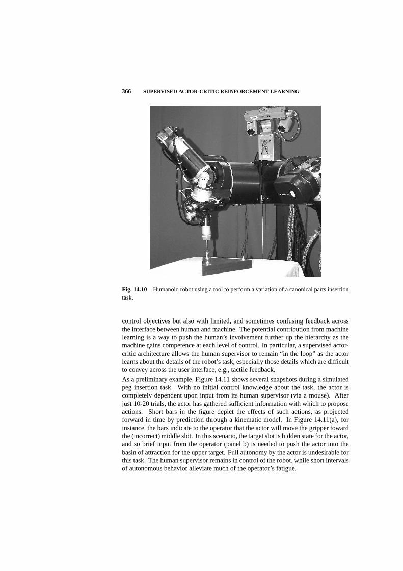
366 SUPERVISED ACTOR-CRITIC REINFORCEMENT LEARNING
Fig. 14.10 Humanoid robot using a tool to perform a variation of a canonical parts insertiontask.
control objectives but also with limited, and sometimes confusing feedback acrossthe interface between human and machine. The potential contribution from machinelearning is a way to push the human’s involvement further up the hierarchy as themachine gains competence at each level of control. In particular, a supervised actor-critic architecture allows the human supervisor to remain “in the loop” as the actorlearns about the details of the robot’s task, especially those details which are difficultto convey across the user interface, e.g., tactile feedback.
As a preliminary example, Figure 14.11 shows several snapshots during a simulatedpeg insertion task. With no initial control knowledge about the task, the actor iscompletely dependent upon input from its human supervisor (via a mouse). Afterjust 10-20 trials, the actor has gathered sufficient information with which to proposeactions. Short bars in the figure depict the effects of such actions, as projectedforward in time by prediction through a kinematic model. In Figure 14.11(a), forinstance, the bars indicate to the operator that the actor will move the gripper towardthe (incorrect) middle slot. In this scenario, the target slot is hidden state for the actor,and so brief input from the operator (panel b) is needed to push the actor into thebasin of attraction for the upper target. Full autonomy by the actor is undesirable forthis task. The human supervisor remains in control of the robot, while short intervalsof autonomous behavior alleviate much of the operator’s fatigue.
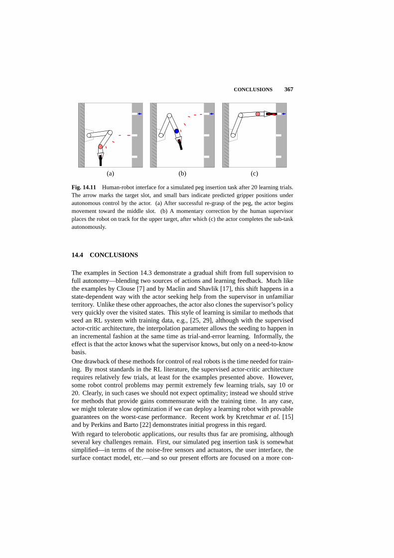
CONCLUSIONS 367
(a) (b) (c)
Fig. 14.11 Human-robot interface for a simulated peg insertion task after 20 learning trials.The arrow marks the target slot, and small bars indicate predicted gripper positions underautonomous control by the actor. (a) After successful re-grasp of the peg, the actor beginsmovement toward the middle slot. (b) A momentary correction by the human supervisorplaces the robot on track for the upper target, after which (c) the actor completes the sub-taskautonomously.
14.4 CONCLUSIONS
The examples in Section 14.3 demonstrate a gradual shift from full supervision tofull autonomy—blending two sources of actions and learning feedback. Much likethe examples by Clouse [7] and by Maclin and Shavlik [17], this shift happens in astate-dependent way with the actor seeking help from the supervisor in unfamiliarterritory. Unlike these other approaches, the actor also clones the supervisor’s policyvery quickly over the visited states. This style of learning is similar to methods thatseed an RL system with training data, e.g., [25, 29], although with the supervisedactor-critic architecture, the interpolation parameter allows the seeding to happen inan incremental fashion at the same time as trial-and-error learning. Informally, theeffect is that the actor knows what the supervisor knows, but only on a need-to-knowbasis.
One drawback of these methods for control of real robots is the time needed for train-ing. By most standards in the RL literature, the supervised actor-critic architecturerequires relatively few trials, at least for the examples presented above. However,some robot control problems may permit extremely few learning trials, say 10 or20. Clearly, in such cases we should not expect optimality; instead we should strivefor methods that provide gains commensurate with the training time. In any case,we might tolerate slow optimization if we can deploy a learning robot with provableguarantees on the worst-case performance. Recent work by Kretchmaret al. [15]and by Perkins and Barto [22] demonstrates initial progress in this regard.
With regard to telerobotic applications, our results thus far are promising, althoughseveral key challenges remain. First, our simulated peg insertion task is somewhatsimplified—in terms of the noise-free sensors and actuators, the user interface, thesurface contact model, etc.—and so our present efforts are focused on a more con-

368 SUPERVISED ACTOR-CRITIC REINFORCEMENT LEARNING
vincing demonstration with the humanoid robot shown in Figure 14.10. Anotherdifficulty is that input from the supervisor can quickly undo any progress made by theRL component. Consequently, we are also exploring principled ways to weaken theeffects of the supervised learning aspect without necessarily weakening the humanoperator’s control over the robot. A third challenge is related to the way a human-robot interface introduces constraints during the learning process. For example, theinterface may restrict the supervisor’s control of the robot to various subsets of itsdegrees of freedom. In turn, this biases the way training data are gathered, such thatthe actor has difficulty learning to coordinate all degrees of freedom simultaneously.
Despite the challenges when we combine supervised learning with an actor-critic ar-chitecture, we still reap benefits from both paradigms. From actor-critic architectureswe gain the ability to discover behavior that optimizes performance. From supervisedlearning we gain a flexible way to incorporate domain knowledge. In particular, theinternal representations used by the actor can be very different from those used bythe supervisor. The actor, for example, can be an artificial neural network, whilethe supervisor can be a conventional feedback controller, expert knowledge encodedas logical propositions, or a human supplying actions that depend on an entirelydifferent perception of the environment’s state. Moreover, the supervisor can conveyintentions and solution strategies to the actor, and so this work is similar in spiritto work on imitation learning, e.g., [19, 26]. And presumably the supervisor has acertain proficiency at a given task, which the actor exploits for improved performancethroughout learning.
Acknowledgments
We thank Andrew Fagg, Mohammad Ghavamzadeh, and Balaraman Ravindran for helpfuldiscussions. This work was supported by NASA under award No. NAG-9-1379. Anyopinions, findings, and conclusions or recommendations expressed in this material are thoseof the authors and do not necessarily reflect the views of the National Aeronautics and SpaceAdministration.
Bibliography
1. J. Albus,Brains, Behavior, and Robotics,Byte Books, Peterborough, NH, 1981.
2. A. G. Barto, “Reinforcement learning in motor control,” In M. A. Arbib, editor,The Handbook of Brain Theory and Neural Networks, Second Edition,pp. 968–972, The MIT Press, Cambridge, MA, 2003.
3. A. G. Barto, R. S. Sutton, and C. W. Anderson, “Neuronlike elements that cansolve difficult learning control problems,”IEEE Transactions on Systems, Man,and Cybernetics,13:835–846, 1983.
4. H. Benbrahim and J. A. Franklin, “Biped dynamic walking using reinforcementlearning,”Robotics and Autonomous Systems, 22:283–302, 1997.
5. N. A. Bernstein,The Co-ordination and Regulation of Movements,PergamonPress, Oxford, 1967.
6. A. E. Bryson and Y.-C. Ho,Applied Optimal Control,Hemisphere PublishingCorp., New York, 1975.
7. J. A. Clouse,On Integrating Apprentice Learning and Reinforcement Learning,PhD thesis, University of Massachusetts, Amherst, 1996.
8. J. A. Clouse and P. E. Utgoff, “A teaching method for reinforcement learn-ing,” Proceedings of the Nineth International Conference on Machine Learning,pp. 92–101, Morgan Kaufmann, San Francisco, CA, 1992.
9. J. J. Craig,Introduction To Robotics : Mechanics and Control,Addison-WesleyPublishing Company, Reading, MA, 1989.
10. M. Dorigo and M. Colombetti, “Robot shaping: developing autonomous agentsthrough learning,”Artificial Intelligence,71(2):321–370, 1994.
11. V. Gullapalli, “A stochastic reinforcement learning algorithm for learning real-valued functions,”Neural Networks,3(6):671–692, 1990.
12. M. Huber and R. A. Grupen, “A feedback control structure for on-line learningtasks,”Robotics and Autonomous Systems,22(3–4):303–315, 1997.
369
370 BIBLIOGRAPHY
13. M. I. Jordan and D. E. Rumelhart, “Forward models: Supervised learning witha distal teacher,”Cognitive Science,16(3):307–354, 1992.
14. M. Kaiser and R. Dillmann, “Building elementary robot skills from humandemonstration,”Proceedings of the IEEE International Conference on Roboticsand Automation,pp. 2700–2705, IEEE, Piscataway, NJ, 1996.
15. R. M. Kretchmar, P. M. Young, C. W. Anderson, D. C. Hittle, M. L. Anderson,C. C. Delnero, and J. Tu, “Robust reinforcement learning control with staticand dynamic stability,”International Journal of Robust and Nonlinear Control,11:1469–1500, 2001.
16. L.-J. Lin, “Self-improving reactive agents based on reinforcement learning, plan-ning and teaching,”Machine Learning,8(3–4):293–321, 1992.
17. R. Maclin and J. W. Shavlik, “Creating advice-taking reinforcement learners,”Machine Learning,22((1-3)):251–281, 1996.
18. M. J. Mataric, “Reward functions for accelerated learning,”Proceedings of theEleventh International Conference on Machine Learning,pp. 181–189, MorganKaufmann, San Francisco, CA, 1994.
19. M. J. Mataric, “Sensory-motor primitives as a basis for imitation: linking per-ception to action and biology to robotics,” In C. Nehaniv and K. Dautenhahn,editors,Imitation in Animals and Artifacts,The MIT Press, Cambridge, MA,2000.
20. A. Y. Ng, D. Harada, and S. Russell, “Policy invariance under reward trans-formations: Theory and applications to reward shaping,” InProceedings of theSixteenth International Conference on Machine Learning,pp. 278–287, MorganKaufmann, San Francisco, CA, 1999.
21. T. J. Perkins and A. G. Barto, “Lyapunov-constrained action sets for reinforce-ment learning,” In C. Brodley and A. Danyluk, editors,Proceedings of the Eigh-teenth International Conference on Machine Learning,pp. 409–416, MorganKaufmann, San Francisco, CA, 2001.
22. T. J. Perkins and A. G. Barto, “Lyapunov design for safe reinforcement learning,”Journal of Machine Learning Research,3:803–832, 2002.
23. B. Price and C. Boutilier, “Implicit imitation in multiagent reinforcement learn-ing,” In I. Bratko and S. Dzeroski, editors,Proceedings of the Sixteenth Interna-tional Conference on Machine Learning,pp. 325–334, Morgan Kaufmann, SanFrancisco, CA, 1999.
24. J. C. Santamaria, R. S. Sutton, and A. Ram, “Experiments with reinforcementlearning in problems with continuous state and action spaces,”Adaptive Behavior,6:163–217, 1997.
BIBLIOGRAPHY 371
25. S. Schaal, “Learning from demonstration,” In M. C. Mozer, M. I. Jordan, andT. Petsche, editors,Advances In Neural Information Processing Systems 9,pp. 1040–1046, The MIT Press, Cambridge, MA, 1997.
26. S. Schaal, “Is imitation learning the route to humanoid robots?""Trends inCognitive Science,3:233–242, 1999.
27. J. S. Shamma, “Linearization and gain-scheduling,” In W. S. Levine, editor,TheControl Handbook,pp. 388–396, CRC Press, Boca Raton, FL, 1996.
28. S. P. Singh and R. S. Sutton, “Reinforcement learning with replacing eligibilitytraces,”Machine Learning,22(1–3):123–158, 1996.
29. W. D. Smart and L. P. Kaelbling, “Effective reinforcement learning for mobilerobots,” Proceedings of the IEEE International Conference on Robotics andAutomation,pp. 3404–3410, 2002. IEEE, Piscataway, NJ.
30. R. S. Sutton, “Learning to predict by the method of temporal differences,”Machine Learning,3:9–44, 1988.
31. R. S. Sutton and A. G. Barto,Reinforcement Learning: An Introduction,TheMIT Press, Cambridge, MA, 1998.
32. C. J. C. H. Watkins and P. Dayan, “Q-learning,”Machine Learning,8(3/4):279–292, 1992.
33. R. J. Williams, “Simple statistical gradient-following algorithms for connection-ist reinforcement learning,”Machine Learning,8:229–256, 1992.
Appendix 1: Nomenclature
a composite actionaA actor actionaE exploratory actionaS supervisor actionα learning step size (actor)β learning step size (critic)δ TD errorE supervisory errore eligibility traceγ discount factork interpolation parameterλ eligibility trace decay factorπ composite policyπA actor policy
πE exploratory policyπS supervisor policyr immediate rewardR expected immediate rewards current states′ next stateσ exploration sizeθ CMAC weight vector (critic)Vπ value function under policyπV estimate ofVπ
w CMAC weight vector (actor)∆wRL reinforcement learning update∆wSL supervised learning update
372 BIBLIOGRAPHY
Appendix 2: Cerebellar Model Arithmetic Computer
A CMAC, or cerebellar model arithmetic computer[1], is a kind of artificial neuralnetwork inspired by the anatomy and physiology of the cerebellum. Much like radialbasis function (RBF) networks, CMACs have processing units that are localized indifferent regions of an input space. In contrast with RBF networks—where eachunit computes a scalar value based on how close an input is to the center of theunit—CMAC units instead compute a binary value for each input. In either case,the computed values affect how much the associated weight parameters contributeto the network’s output. With CMAC units, their binary nature therefore deter-mines whether a particular weight “participates” entirely or not at all in the outputcalculation.
Also in contrast to RBF networks—with radially symmetric processing units—CMAC units are hyper-rectangles arranged as atiling, i.e., as a grid-like tessellationof the input space. This leads to computationally efficient implementations similarto lookup tables. Another advantage of CMACs is that multiple tilings, with eachone offset from the rest, can be used to improve resolution, while relatively largehyper-rectangles can be used to improve generalization. And for modern RL algo-rithms, a function approximator with binary units allows one to take advantage ofreplacing eligibility traces [28], as we do with the algorithm in Figure 14.3. See [24]for more information about CMACs, including an empirical evaluation of their usefor RL problems.
15 BPTT and DAC:A Common Framework forComparison
DANIL V. PROKHOROV
Ford Motor Company
Editor’s Summary: This chapter compares and contrasts derivative adaptive critics(DAC) such as dual heuristic programming (DHP), which was first introduced inChapter 1 and also discussed in Chapter 3 with back-propagation through time(BPTT). A common framework is built and it is shown that both are techniques fordetermining the derivatives for training parameters in recurrent neural networks. Thischapter goes into sufficient mathematical detail that the reader can understand thetheoretical relationship between the two techniques. The author presents a hybridtechnique that combines elements of both BPTT and DAC and provides detailedpseudocode. Computational issues and classes of challenging problems are discussed.
15.1 INTRODUCTION
Heterogeneous ordered networks or, more specifically, recurrent neural networks(RNN) are convenient and flexible computational structures applicable to a broadspectrum of problems in system modeling and control. They require efficient algo-rithms to achieve successful learning for the given task. Backpropagation throughtime (BPTT), henceforth assumed to be its truncated version with a sufficient depthof truncation, and derivative adaptive critics (DAC) are two seemingly quite differentapproaches to solve temporal differentiable optimization problems with continuousvariables. In fact, both BPTT and DAC are means to obtain derivatives for trainingparameters of RNN.
We show that both approaches are related. BPTT is used in DAC to obtain targetsfor derivative critic adaptation in RNN training. DAC can be interpreted as a methodto reduce the need for introducing a potentially large truncation depth in BPTT byproviding estimates of derivatives from the future time steps. This realization allows
373
374 SAMPLE SHORT VERSION OF TITLE FOR RUNNING HEAD
us to establish a common framework for comparison of derivatives of BPTT andthose of DAC and summarize their differences. The main difference stems fromthe fact that derivatives provided by DAC are learned via a representation (criticnetwork), and such derivatives can be averages of derivatives provided by BPTT. Itshould be kept in mind that some derivative averaging naturally occurs in the trainingprocess during which RNN parameters are being adjusted (usually incrementally).Depending on the problem setup and critic training mechanics, DAC derivatives mayor may not be sufficiently accurate for successful RNN training.
Both BPTT and DAC must also be equipped with a parameter adjustment rule oralgorithm. BPTT equipped with various forms of the Kalman filter algorithm hasshown its power in tackling difficult RNN training problems. Training a single RNNto model or control multiple systems with its weights fixed upon completion of thetraining is particularly remarkable because it defies successful applications of feed-forward or time-delay NN. In spite of several successful demonstrations of DAC andin contrast to BPTT, DAC has mostly been restricted to training feed-forward NN(neurocontrollers) using a gradient descent rule. It is crucial for DAC to reinforceitself with more powerful architectures and training algorithms to be capable ofsolving truly difficult optimization problems.
Sufficiently detailed comparisons between BPTT and DAC as training approachesto RNN are essentially lacking. Careful comparisons should be based not onlyon the results of comprehensive testing of the solutions but also on assessments ofthe computational requirements of the approaches. It is noteworthy that the criticnetwork is discarded as soon as RNN parameter training is finished, which is wasteful.Furthermore, comparisons for a clearly formulated and easily accessible modelingproblem may be preferable over comparisons for control problems because modelingproblems usually have a relatively simple setup. We suggest a nonstationary systemmodeling problem as a possible benchmark for comparing BPTT and DAC.
This chapter is structured as follows. In Section 15.2 we show a relationship betweenBPTT and DAC that gives rise to a common framework for comparison of the twomethods. In Section 15.3 we discuss critic representation. In Section 15.4 we proposea hybrid between BPTT and DAC which can be useful for comparative studies. InSection 15.5 we emphasize the need to base comparisons of the two methods notonly on the final result but also on computational requirements for each method.We discuss two classes of challenging problems which could form a core of futurecomparative studies of BPTT and DAC in Section 15.6.
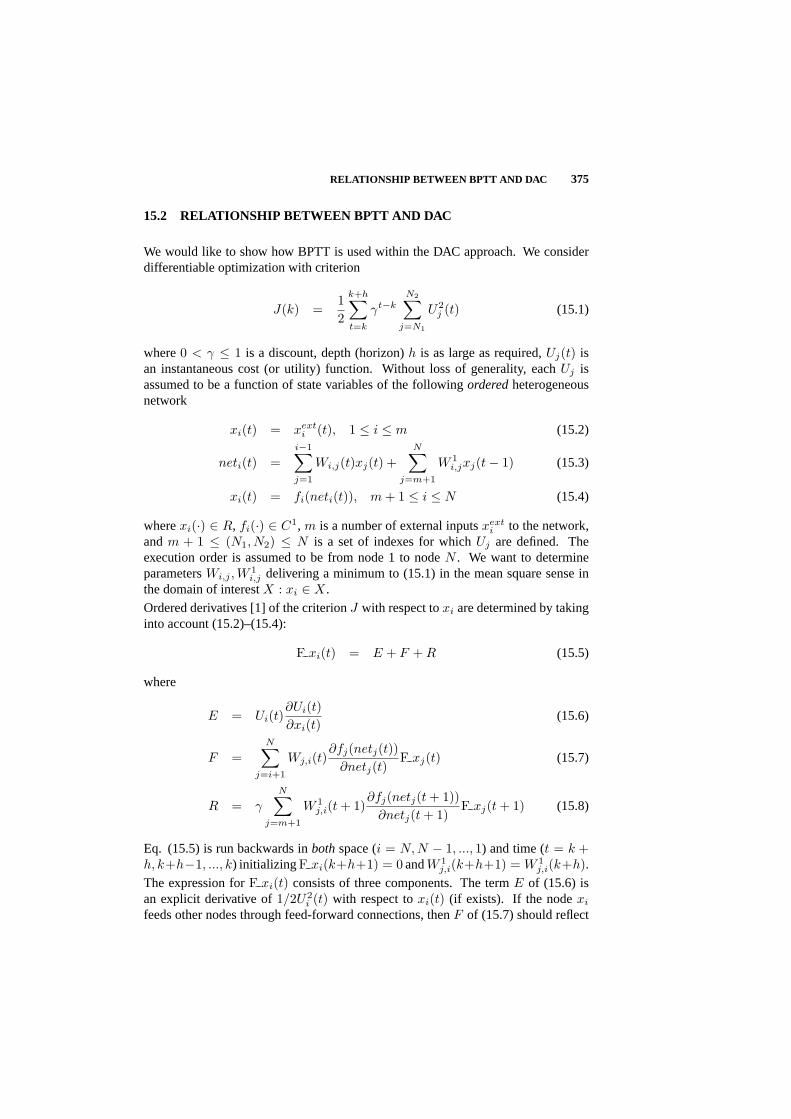
RELATIONSHIP BETWEEN BPTT AND DAC 375
15.2 RELATIONSHIP BETWEEN BPTT AND DAC
We would like to show how BPTT is used within the DAC approach. We considerdifferentiable optimization with criterion
J(k) =12
k+h∑
t=k
γt−kN2∑
j=N1
U2j (t) (15.1)
where0 < γ ≤ 1 is a discount, depth (horizon)h is as large as required,Uj(t) isan instantaneous cost (or utility) function. Without loss of generality, eachUj isassumed to be a function of state variables of the followingorderedheterogeneousnetwork
xi(t) = xexti (t), 1 ≤ i ≤ m (15.2)
neti(t) =i−1∑
j=1
Wi,j(t)xj(t) +N∑
j=m+1
W 1i,jxj(t− 1) (15.3)
xi(t) = fi(neti(t)), m + 1 ≤ i ≤ N (15.4)
wherexi(·) ∈ R, fi(·) ∈ C1, m is a number of external inputsxexti to the network,
andm + 1 ≤ (N1, N2) ≤ N is a set of indexes for whichUj are defined. Theexecution order is assumed to be from node 1 to nodeN . We want to determineparametersWi,j ,W
1i,j delivering a minimum to (15.1) in the mean square sense in
the domain of interestX : xi ∈ X.
Ordered derivatives [1] of the criterionJ with respect toxi are determined by takinginto account (15.2)–(15.4):
F xi(t) = E + F + R (15.5)
where
E = Ui(t)∂Ui(t)∂xi(t)
(15.6)
F =N∑
j=i+1
Wj,i(t)∂fj(netj(t))
∂netj(t)F xj(t) (15.7)
R = γ
N∑
j=m+1
W 1j,i(t + 1)
∂fj(netj(t + 1))∂netj(t + 1)
F xj(t + 1) (15.8)
Eq. (15.5) is run backwards inbothspace (i = N, N − 1, ..., 1) and time (t = k +h, k+h−1, ..., k) initializing F xi(k+h+1) = 0 andW 1
j,i(k+h+1) = W 1j,i(k+h).
The expression forF xi(t) consists of three components. The termE of (15.6) isan explicit derivative of1/2U2
i (t) with respect toxi(t) (if exists). If the nodexi
feeds other nodes through feed-forward connections, thenF of (15.7) should reflect

376 SAMPLE SHORT VERSION OF TITLE FOR RUNNING HEAD
all such connections. Likewise,R of (15.8) reflects all time-delayed connectionsthrough which the nodexi feeds others.
Ordered derivatives with respect to parametersW andW1 are determined usingF xi(t) and (15.2)–(15.4):
F Wi,j(t) = F xi(t)∂fi(neti(t))
∂neti(t)xj(t) (15.9)
F W 1i,j(t) = F xi(t)
∂fi(neti(t))∂neti(t)
xj(t− 1) (15.10)
Eqs. (15.5)–(15.10) are called BPTT [1]. Here they express a truncated form ofBPTT, henceforth denoted as BPTT(h) [2].
Updates of parametersW and W1 can be made by using∑tf
t=t0F Wi,j(t) and∑tf
t=t0F W 1
i,j(t), respectively, wheret0, tf are suitably chosen time steps of thetrajectory (e.g.,t0 = k, tf = k + h, another possibility ist0 = tf = k).
We now consider another optimization criterion (cf. (15.1)):
J ′(t) =12
N2∑
j=N1
U2j (t) + γJ ′(t + 1) (15.11)
The criterionJ of (15.1) is an approximation ofJ ′ which becomes increasingly moreaccurate for sufficiently largeh andγ < 1. On the other hand, the criterion (15.11)is approximated byJ critic in approximate (heuristic) dynamic programming [3].
Let us examine derivatives ofJ ′(t) with respect toxi(t) taking into account (15.2)–(15.4):
λ′i(t) = E′ + F ′ + R′ (15.12)
where
E′ = Ui(t)∂Ui(t)∂xi(t)
(15.13)
F ′ =N∑
j=i+1
Wj,i(t)∂fj(netj(t))
∂netj(t)λ′j(t) (15.14)
R′ = γ
N∑
j=m+1
W 1j,i(t + 1)
∂fj(netj(t + 1))∂netj(t + 1)
λ′j(t + 1) (15.15)
whereλ′j ≡ ∂J ′/∂xi. Note that Eq. (15.12) isnearly identical to (15.5) expressingbackpropagation between two consecutive moments in time (BPTT(1)) [4]. (Re-placingλ′i(t) andλ′j(t + 1) in (15.12),(15.14),(15.15) withF xi(t) andF xj(t + 1),respectively, makes them identical.) Eqs. (15.9)–(15.10) may also be used forminimization of (15.11) except thatF xi(t) should be replaced byλ′i(t).
RELATIONSHIP BETWEEN BPTT AND DAC 377
In a popular DAC approach calleddual heuristic programming(DHP), eachλ′i is tobe approximated by outputλi of λ critic [3]. One can demonstrate that traditionalDHP equations (see, e.g., equations (7) and (8) in [5]) are a special case of (15.12).Theλ critic is expressed as a suitable representationλ(x(t),WC) with outputsλi(·)and adjustable weightsWC . The critic is supposed to be trained with the errorbetweenλ′i(t) from (15.12) and its corresponding outputλi(t). (Eachλ′j(t + 1) in(15.15) is replaced by the appropriate outputλj(t + 1) of the critic.)
We just revealed the similarity between a particular form of BPTT and a popularDAC formulation for the network (15.2)–(15.4), but this is also valid for much moregeneral networks (see [4] and Section 15.4 of this chapter) and systems includingthose with distributed parameters [6]. Recognizing this similarity enables us to createa hybrid of BPTT and DAC in which DAC may act as a means to reduce depthh inBPTT(h) by providing estimates of derivatives from the future time steps (see Section15.4).
Many researchers have pointed out similarities between BPTT and the Euler-Lagrange/Hamiltonian formulation (see, e.g., [19, 17]). The expression (15.12) or (15.5) maybe recognized as the Lagrange multipliers (partial derivatives of a Hamiltonian withrespect to state variables) for the network (15.2)–(15.4) with the criterion (15.11)[18, 17]. The derivatives (15.9), (15.10), or partial derivatives of a Hamiltonian withrespect to controlsW andW1, can be used to update incrementally the networkparameters in order to minimize the criterion (15.11).
We describe a typical application of BPTT to functional minimization. First, weinitialize the state variables of (15.2)–(15.4). We run (15.2)–(15.4) forward forone or more time steps and compute the appropriate values ofU(t) : U(t), U(t +1), ..., U(t + k), whereU is a known function of state variables and their targets(e.g.,U is a tracking error). We then compute the derivatives according to (15.5)by backpropagating fromt + k to t (BPTT(k)) and perform the incremental updatesbased on (15.9) and (15.10).
Compared to this description of BPTT application, the DAC approach requires theutilization of only two adjacent time steps,t andt + 1, according to (15.12). We run(15.2)–(15.4) forward for one time step, obtainU(t), and invoke (15.12) to prepare forcritic training. The right-hand side of (15.12) serves as both the set of instantaneoustargets for critic training and the input to the parameter updates (15.9) and (15.10) (inplace ofF xi(t)). If gradient descent is employed, critic training is also incremental,and it may be based on the expression(λ′i(t)− λi(t))
∂λi(t)WC
, whereWC is a vectorof critic weights.
For either the BPTT or the DAC approach, we continue the training process for thenext pointt + 1 along the trajectory. We can train for a segment of the trajectory,then reinitialize the state variables (15.2)–(15.4) and move on to training on anothersegment of the trajectory. Meanwhile, our weightsW, W1 (andWC for DAC) serveas the long-term memory, incorporating the effects of adaptation averaged over manyinstances. For an adequately chosen training strategy, we can reasonably expect thatapplication of BPTT or DAC will result in the triplet(W,W1,WC)∗ such thatJ isapproximately minimized overX. As with any numerical and (generally) nonconvex
378 SAMPLE SHORT VERSION OF TITLE FOR RUNNING HEAD
optimization, all we can guarantee is that the proper training process should result inattaining a local minimum ofJ (most of the time such a minimum is satisfactory).What is proper remains problem dependent, but determining the training strategyincludes choosing training parameters (e.g., learning rates) for updates based on (15.9)and (15.10), the length and the assignment of trajectory segments and the initializationof state variables. For DAC we need to add the choice of critic training parametersand the coordination scheme between critic and network training processes [15, 4].
The training process based on BPTT also resembles a form of model predictive control(MPC) with receding horizon (see, e.g., [20]). As in the MPC, we run the systemforward for several time steps collecting values ofU . Our horizon (t + k) recedesonce the weight updates are carried out except that our updates are incremental, not“greedy" as in the receding-horizon MPC.
We summarize the differences between derivatives obtained by BPTT and those ofDAC [7]:1) BPTT derivatives are computed directly, while critic derivatives are computedfrom a representation, e.g., a neural network, with its parameters to be learned.2) BPTT(h) derivatives generally involve a finite time horizon (equal to the chosentruncation depthh), while critic derivatives are estimates for an infinite horizon; itis not uncommon, however, to employ a discount factor in (15.11), which may beinterpreted as a gentle truncation (γ < 1). Largeh are permissible because BPTTcomputations scale linearly withh, but frequently smallh (h < 10) suffice.3) BPTT derivatives necessarily compute the effect of changing a variable in thepast, while a derivative critic may be used to estimate the effect of a change at thepresent time. If critics are used only to adjust network parameters, this distinctionis irrelevant . On the other hand, recognizing it poses interesting possibilities foralternative or supplementary methods of control, as discussed in Section 6 of [7].4) A BPTT derivative is essentially exact for the specific trajectory for which it iscomputed, while a critic derivative necessarily represents an average of some kind,e.g., an average over trajectories that begin with a given system state. Such anestimate may be quite accurate (if the critic has been well adapted or trained andif exogenous inputs to the system are either small or statistically well behaved) ormay be essentially worthless (if future operation is completely unpredictable due toarbitrary inputs or targets).
Item 4 is discussed in more details in the next section.
15.3 CRITIC REPRESENTATION
Critic predicts the effect of a change in a variable of the system or network (15.2)–(15.4) on its future operation. Critic is thus a function of the system state, and it isimportant to include in critic representation as much information as available aboutthe system. What is encompassed by the system depends on the context. In thecontext of indirect model reference adaptive control [8], the system is interpretedquite generally as consisting of: 1) controller network, 2) reference model, 3) object
CRITIC REPRESENTATION 379
to be controlled (plant), and 4) model of the plant. State variables or their estimatesof all of these components should be provided as inputs to the critic (the plant modeloften serves as the plant state estimator). However, the only adjustable quantities arethe weights of controller and (sometimes) parameters of the model.
It is convenient to consider all main components of the control system as partsof a singleheterogeneous recurrent network, perhaps similar to (15.2)–(15.4). Thisviewpoint equates control problems with modeling problems (employing RNN) sinceboth types of problems feature feedback.
In the modeling context, we suggest connecting all recurrent nodes or time-delayedelements to the critic because they reflect thestateof the system. In the examplebelow we illustrate that adding a state variable is indeed beneficial [4].
Consider a system
x(k + 1) = xext(k + 1) + wx(k) (15.16)
xd(k + 1) = xext(k + 1) + wdx(k) (15.17)
where0 < |w| < 1, 0 < |wd| < 1, andxext(k), ∀k are i.i.d. random variableswith the same meanxext. The system (15.16)-(15.17) is a simple illustration of thenetwork (15.2)–(15.4), with the controller part expressed as (15.16). The Eq. (15.17)is an example of the reference model, and it describes the desired behavior of (15.16).
The minimization criterion is
J(k) =12
∞∑t=0
γtU2(k + t) =12
∞∑t=0
γt(xd(k + t)− x(k + t))2 (15.18)
DifferentiatingJ(k) with respect tox(k) yields
F x(k) =∞∑
t=0
(γw)t(x(k + t)− xd(k + t)) (15.19)
Substituting (15.16) and (15.17) into the equation forF x(k) above, averaging for allxext(·) and recognizing appropriate power series results in
< F x(k) > =x(k)
1− γw2− xd(k)
1− γwwd
+xextγw
1− γw
(1
1− γw2− 1
1− γwwd
)(15.20)
where< F x(k) > is an (ensemble) average ordered derivative ofJ(k) with respectto x(k).We wish to show that a linearλ critic is sufficient to recover< F x(k) >. The criticrepresentation is
λ(t) = Ax(t) + Bxd(t) + C (15.21)

380 SAMPLE SHORT VERSION OF TITLE FOR RUNNING HEAD
whereA, B, andC are the critic weights. Similar to (15.12), we can write
λ(t) = E′ + R′ (15.22)
where
E′ = x(t)− xd(t) (15.23)
R′ = γλ(t + 1)∂x(t + 1)
x(t)(15.24)
Here (15.23) corresponds to (15.13), and (15.24) corresponds to (15.15) (there isno feed-forward part like (15.14)). Substituting the representation (15.21) into theequation forλ(t) above yields
Ax(t) + Bxd(t) + C = x(t)− xd(t)+γw(Ax(t + 1) + Bxd(t + 1) + C) (15.25)
When the weights converge they become
A =1
1− γw2(15.26)
B = − 11− γwwd
(15.27)
C =xextγw
1− γw
(1
1− γw2− 1
1− γwwd
)(15.28)
which, incidentally, indicates that< F x(k) > is restored exactly.
A reasonable question to ask is what happens if we do not have access to state(s)of the data generator/reference modelxd. Such situation may happen when traininga recurrent network from a file of input-output pairs. We suggest approximatingthe states of the missing reference model by its time-delayed outputs and providethese estimates as inputs to the critic. (The order of the system which produced thetraining data might be known and used to determine how many time-delayed inputsto employ.)
One can certainly argue that even a simpler critic representation lacking some difficult-to-find inputs might suffice for a problem at hand. However, we should keep in mindthat excluding a state or its estimate from the critic input set effectively turns such astate into a disturbance which tends to decrease the likelihood of getting an accuratecritic and handicaps the critic as compared to BPTT.
Many representations for critics are possible. For example, each output can be aseparate function or neural networkλi(x(t),WC). In the example above we usedthe linear critic. Extremely simple (bias weight only) representations are also viablefor some problems [9], as illustrated below.
CRITIC REPRESENTATION 381
Consider the following system
x1(t) = bxext(t) (15.29)
x2(t + 1) = x1(t) (15.30)
x3(t + 1) = 0.5x3(t) + x1(t + 1) + xext(t + 1)− 2x2(t) (15.31)
or, in a compact form,
x3(t + 1) = 0.5x3(t) + (1 + b)xext(t + 1)− 2bxext(t− 1) (15.32)
The reference inputxext has a piecewise constant pattern with a long enough dwelltime (e.g., 50 time steps). The goal is to adjust the parameterb so as to minimize(xd
3(t)−x3(t))2, wherexd3(t) ≡ 0, ∀t, in the mean square sense in which caseb = 1.
BPTT(2) must be used to accomplish this (the training process diverges if BPTT(h)with h < 2 is used).
We show how the use of two DAC (λ) critics eliminates the need for more than the(computational) equivalent of BPTT(1). The BPTT equations for this system aresimilar to (15.5):
F x3(t) = −e(t) + 0.5F x3(t + 1) (15.33)
F x2(t) = −2F x3(t + 1) (15.34)
F x1(t) = F x3(t) + F x2(t + 1) (15.35)
wheree(t) = 0 − x3(t) = −x3(t). In the first equation−e(t) is equivalent to(15.6), and0.5F x3(t+1) is equivalent to (15.8) (it is obtained from the equation forx3(t + 1)). The equation forx3(t + 1) is also used to obtainF x2(t) andF x3(t) inthe expression forF x1(t). The last equation (forF x1(t)) is obtained by combiningF x1(t) = F x2(t + 1) with F x1(t + 1) = F x3(t + 1) at timet.
The BPTT equations above are to be repeated two times (BPTT(2)) to produceF x1
suitable for updatingb correctly:
F b(t) = F x1(t)xext(t) (15.36)
According to (15.12), we replaceF x3(t + 1) andF x2(t + 1) with λ3(t + 1) andλ2(t + 1), respectively, and obtain
λ′3(t) = −e(t) + 0.5λ3(t + 1) (15.37)
λ′2(t) = −2λ3(t + 1) (15.38)
F x1(t) = λ′3(t) + λ2(t + 1) (15.39)

382 SAMPLE SHORT VERSION OF TITLE FOR RUNNING HEAD
whereF x1(t) is used in (15.36) to updateb. It turns out that the bias-weight-onlycritics suffice for this problem, and they may be updated as follows
λ3 + = η(λ′3(t)− λ3) (15.40)
λ2 + = η(λ′2(t)− λ2) (15.41)
where learning rateη > 0 is reasonably chosen, and the C-language notation “+=”indicates that the quantity on the right hand side is to be added to the previouslycomputed value of the left hand side. It can be shown that performing updates of thecritics and the weightb results in convergence ofb to its desired value of unity if thesystem is sufficiently excited byxext.
The system (15.32) could easily be changed to representD delays which would eitherrequire BPTT(D) orD critics trained in a fashion similar to this example.
As illustrated with the example (15.29)–(15.41), even a trivial critic can be effectiveand competitive with BPTT when dealing with a predictable system. (A goodexample of a predictable system is a system with a constant (or fixed-statisticsrandom) disturbance.) The system above is predictable because it is driven by aslowly-varying excitation. However, any critic-based training approach will havedifficulties if the system is subject toxext changing significantly at every time step.For this and other systems with recurrence and block delays affected by fast-changingdisturbances or excitations it is better to use a hybrid of temporal backpropagation[10], BPTT and, possibly, DAC proposed in [11].
15.4 HYBRID OF BPTT AND DAC
Here we provide the reader with C-language-style pseudocode describing a hybridof BPTT and DAC which is less efficient in handling block delays than that in [11]but easier to implement.
The forward equations for an ordered network withn in inputs andn out outputsmay be expressed very compactly in a pseudocode format [13]. Let the networkconsist ofn nodes nodes, of whichn in serve as receptors for the external inputs.The bias input, which we denote formally as node 0, is not included in the nodecount. The bias input is set to the constant 1.0. The arrayI contains a list of theinput nodes; e.g.,Ij is the number of the node that corresponds to thejth input, inj .Similarly, a list of the nodes that correspond to network outputs outp is contained inthe arrayO. We allow network outputs and targets to be advanced or delayed withrespect to node outputs by assigning a phaseτp to each output. For example, if wewish to associate the network outputp with the output of some system five steps inthe future, we would haveτp = 5. Nodei receives input fromn con(i) other nodesand has activation functionfi(·); n con(i) is zero if nodei is among the nodeslisted in the input arrayI . The arrayc specifies connections between nodes;ci,j isthe node number for thejth input of nodei. Inputs to a given node may originate
HYBRID OF BPTT AND DAC 383
at the current or past time steps, as specified by delays contained in the arrayd, andthrough weights for time stept contained in the arrayW(t).Prior to beginning network operation, all appropriate memory is initialized. Normally,such memory will be set to zero. (In some cases memory that corresponds to thenetwork initial state may be set to specified values.)
At the beginning of each time step, we execute the following buffer operations onweights and node outputs (in practical implementation, a circular buffer and pointerarithmetic may be employed). Heredmax is the largest value of delay represented inthe arrayd, andh is the truncation depth of the BPTT gradient calculation describedin a pseudocode form later.
for i = 1 to n nodes for it = t-h-dmax to t-1
W(it) = W(it + 1) (15.42)
yi(it) = yi(it + 1) (15.43)
/* end it loop */ /* end i loop */
Then, the actual network execution is expressed as
for i = 1 to n in
yIi(t) = ini(t) (15.44)
for i = 1 to n nodes if n con(i) > 0
ai(t) =
[ ∑n con(i)j=1 Wi,j(t)yci,j (t− di,j)∏n con(i)
j=1 (Wi,j(t) + yci,j (t− di,j))
]. (15.45)
yi(t) = fi
(ai(t)
)(15.46)
for p = 1 to n out
outp(t + τp) = yOp(t) (15.47)
Most commonly, we take the (differentiable) activation functionfi(·) to be either

384 SAMPLE SHORT VERSION OF TITLE FOR RUNNING HEAD
linear or a bipolar sigmoid, though we also can make use of other functions, e.g.,sinusoids, for special purposes. In the pseudocode above, the top portion of theright-hand side of (15.45) is invoked whenever the nodei performs a summation ofits inputs weighted by the appropriate elements ofW. The bottom portion of theright-hand side of (15.45) is invoked if the nodei is a product (multiplicative) node.
The pseudocode above is very general, and it can be used to describe a great deal ofneural and non-neural computational structures including (15.2)–(15.4).
In the pseudocode for a hybrid ofaggregateBPTT [12] and DAC below,Fpy denotes
an ordered derivative of12∑h
ih =0 γih (Up(t− h + ih ))2 (cf. (15.1)), whereUp is acomponent of the utility vectorU usually expressed as a deviation between appro-priate target and output of the network. This pseudocode can be invoked at each timestep only after the completion of forward propagation at time stept.
for p = 1 to n out for i = 1 to n nodes for k = 1 to n con(i)
FpWi,k = 0 (15.48)
/* end k loop */for it = t to t-h-dmax
Fpyi(it) = 0 (15.49)
if it = t
Fpyi(it) = κp
i (it) (15.50)
/* end it loop */ /* end i loop */for ih = 0 to h
i1 = max(t− ih, 0) (15.51)
Up(i1) = tgtp(i1 + τp)− outp(i1 + τp) (15.52)
FpyOp(i1) + = −Up(i1) (15.53)
for i = n nodes to 1 if n con(i) > 0

HYBRID OF BPTT AND DAC 385
for k = n con(i) to 1
j = ci,k (15.54)
i2 = max(i1 − di,k, 0) (15.55)
Fpyj(i2) + = γdi,kF
pyi(i1)f ′i(ai(i1))
×[
Wi,k(i1)∏n con(i)m=1,m6=k(Wi,m(i1) + yci,m
(i1 − di,m))
].(15.56)
FpWi,k + = F
pyi(i1)f ′i(ai(i1))
×[
yj(i2)∏n con(i)m=1,m 6=k(Wi,m(i1) + yci,m
(i1 − di,m))
]. (15.57)
/* end k loop */ /* end i loop */ /* end ih loop */ /* end p loop */
The loops for (15.48) and (15.49) serve as initializations. We useκpi to denote
the outputi of derivative critic for componentp of the utility vectorU. This is doneto avoid confusion withλi discussed above.
By virtue of “+ =” notation, the appropriate derivatives are distributed from agiven node to all nodes and weights that feed it in the forward direction, with dueallowance for any delays that might be present in each connection. The simplicityof the formulation reduces the need for visualizations such as unfolding in time orsignal-flow graphs.
If the nodei is one of the summation nodes (as in the top portion of the right-hand sideof (15.45)), then the derivatives with respect toyj andWi,k are computed accordingto the top portions of the left-bracketed terms in (15.56) and (15.57), respectively.For a multiplicative node (as in the bottom portion of the right-hand side of (15.45)),these derivatives are computed according to the bottom portions of the left-bracketedterms in (15.56) and (15.57).
DAC errors and targets are computed after completion of the pseudocode above:
for p = 1 to n out for i = n nodes to 1 if n con(i) > 0

386 SAMPLE SHORT VERSION OF TITLE FOR RUNNING HEAD
for k = n con(i) to 1
j = ci,k (15.58)
i2 = t− h− di,k (15.59)
κ∗pj (i2) = Fpyj(i2) (15.60)
εpj (i2) = κ∗pj (i2)− κp
j (i2) (15.61)
/* end k loop */ /* end i loop */ /* end p loop */
A special case withh = 0 and dmax = 1 is what may be called the pure DACalgorithm (cf. Eq. (15.12)). However, there is one crucial difference. In the usualformulation (15.12), derivative critics designated byλ are trained to estimate deriva-tives ofJ ′, including the contribution from the current step,k. The pseudocode aboveseparates the estimate of the future from that of the present, and it is a generalizationof the algorithm proposed in [14] (cf.C critics in [14]).
The difference between the values of the two critic forms is precisely the quantity thatresults when the derivative of error at each output node∂J ′
∂yout(k) is backpropagatedto y(k). (In the simple case of a single-node network, the new criticκ(k) is relatedto the usual critic as follows:λ(k) = ∂J ′
∂y(k) +κ(k).) Theκ critic is thus not requiredto estimate quantities which can be computed exactly. Limited experimentationsuggests that the use ofκ critics may lead to faster training than that ofλ critics.
Critic can be trained using the error (15.61). For example, a gradient descent updateof critic weights may look like this:
WpC + = ηpεp
j (t− 1)∂κp
j (t− 1)∂Wp
C
(15.62)
whereWpC is a vector of weights of the criticp, andηp > 0 (h = 0 anddmax =
1). (We assume in (15.62) that an individual critic is used to approximate orderedderivatives of the discounted sum ofU2
p with respect to node outputyj . One canalso combine all such critics into one network.) The critic outputs may correspond todifferent time steps whendi,k is different for different RNN nodes, as follows from(15.61).
No critic training happens if all critic outputsκpj and their learning rates are fixed at
zero. In such a case, our pseudocode amounts to carrying out the aggregate BPTT(h).If the gradient descent training of weightsW is desired, then we useF
pWi,k of
(15.57) to adjustWi,k(t). For extended Kalman filter (EKF) training [13], the errorinjection (15.53) should be modified for consistency with mechanics of the EKFrecursion (see [12]).
COMPUTATIONAL COMPLEXITY AND OTHER ISSUES 387
If h > 0 and critic training is enabled, then (15.62) may be invoked to train thecritic (alternatively, the EKF algorithm can be used). While limited experiments withutilizing derivatives (15.57) in conjunction with EKF updates have been carried outsuccessfully, further experimentation is needed since such derivatives are differentfrom those usually employed by the EKF, especially when backpropagation to theRNN weights, as in (15.57), is performed only fori1 = t− h [14].
Concluding this section, it should be mentioned that our hybrid can be used evenwhen components ofU are not defined for all time steps. Furthermore, a differen-tiable approximation ofU may be used if the trueU is not well defined. Such anapproximation capturing an essential relationship between the network variables andthe desired instantaneous utility or the final outcome (e.g., in a game setting) couldbe learned in a separate training task prior to invoking the hybrid equations of thissection [7].
15.5 COMPUTATIONAL COMPLEXITY AND OTHER ISSUES
We wish to compare the overhead associated with computations ofF Wi,j andκi forDAC with the cost of computingF Wi,j for BPTT(h).
We assume that the cost of forward and back-propagations through a network isdominated by a linear term proportional to the number of its weights. For a criticwith NWC weights, the cost of carrying out static BP (BPTT(0)) isO(NWC ). If weuse totalNC data points to train a critic, the critic training cost is proportional to bothNWC andNW because backpropagation through a RNN withNW weights to obtaincritic targets (15.61) hasO(NW) complexity for each ofNC data points. Traininga network with DAC onNA data points incurs a cost proportional to bothNW andNWC
because the critic is to be executed withO(NWC) complexity for each ofNA
data points. Thus, the total computational cost of DAC algorithm is proportional to(NC + NA)NWC and(NC + NA)NW.
The cost of BPTT(h) isO(NWh). If we useNB data points to train the network,then the total cost is proportional toNBNWh.
Our simple analysis does not take into account the cost of updatingW in both thenetwork and the critic which can be significant, especially for second order methods.Let us assume that the network weight updating incurs the same cost for both methods.If
α(NC + NA)NWC + β(NC + NA)NW + WC update cost < ωNBNWh
(15.63)
whereα, β, ω are some problem-dependent constants, then the DAC approach is moreefficient computationally than the BPTT(h) approachprovided that the updates ofW result in the same network performance upon completion of its training.
388 SAMPLE SHORT VERSION OF TITLE FOR RUNNING HEAD
It appears possible to simplify the DAC approach for some problems, e.g., when thesystem is affine in controlsa:
x(t + 1) = F(x(t)) + G(x(t))a(t) (15.64)
whereF is a vector function,G is a control matrix. IfU(t) is quadratic ina,i.e., includes the termaT (t)Ra(t), R > 0, then implementable parameterization ofthe optimal controller may be expressed using the criticλ (vector) as the followingproduct
a(t) = −R−1GT (x(t))λ(x(t),WC) (15.65)
Thus unlike the usual DAC approach featuring training of two entities (critic andcontroller), no controller training is necessary here. In such a case the expression forcomputational cost comparison above is changed to
ζNCNWC+ WC update cost < ωNBNWh (15.66)
whereζ is another constant.
Derivatives from DAC (values ofλi or κi) represent averages of derivativesF xi, asshown in the example (15.16)–(15.28). That example also touches upon the followingimportant issue. To obtain the accurate average< F x(k) >, we have to wait untilconvergence of critic weightsA,B andC. Even more importantly, the parametersw andwd must be kept fixed. If training ofw is in progress (orwd is changing),critic accuracy will also depend on how these parameters are being changed, becauseevery change inw or wd results in a change to the system or network to which thecritic is being adapted. In a general case of many weights changing in a network,if their updates are to be closely interleaved with critic updates, a relatively simplecritic representational structure might be warranted, so that the critic can be quicklyadapted to changes in the system.
The proper coordination of critic training with network (controller) training has beena research topic. We have found that, in some cases, it is possible to update bothnetwork weights and critic weights at every training step, although such a strategymay not work well in the presence of network weight updates of larger size, asfrequently result from second order training procedures. Alternating the trainingprocesses in blocks is a reasonable option, since holding the network fixed whileadapting the critic generally leads to greater critic accuracy. The drawback is thatonce the critic is held fixed and the network is changed, the critic may become veryinaccurate and compromise training with poor derivatives. Hence a better approachmight be to carry out the training processes concurrently but to monitor the critic error(the error used to update the critic) and to suspend network training for some numberof steps if a specified critic error is exceeded. Of special interest are case studiesin [15, 16] where various alternatives for coordinated updates of critic and networkhave been analyzed. One alternative includes training of more than one critic (termed“shadow critic/controller" method), with periodic alternations between the critics to
TWO CLASSES OF CHALLENGING PROBLEMS 389
improve convergence. Yet, no comparison from the standpoint of computational costakin to the analysis of this section have been made.
Efficiency of critic adaptation is paramount because the critic is discarded as soonas the controller training is finished. Interestingly, very few attempts have beenmade to analyze critic training accuracy or critic usability after obtaining the requiredcontroller. As for the latter, we discuss the use of a critic to analyze Lyapunovstability of the closed-loop system in [21].
15.6 TWO CLASSES OF CHALLENGING PROBLEMS
BPTT(h) equipped with EKF algorithm [13] has shown its power in dealing withdifficult training problems requiring the use of RNN. Recently progress has beenmade in nonlinear Kalman filters in a joint estimation framework with promise toeliminate not only BPTT but also the necessity to calculate derivatives in the system.Currently the new method’s only drawback is extra complexity as compared to thatof the standard EKF method [22].
More challenging of RNN training problems solved with Kalman filter methods canbe categorized in two broad classes [23]. Class I encompasses neural approximationof multiple input-output mappings of the following form
yd(t) = fθ(zθ(t− 1),xθ(t)) (15.67)
wherefθ is a discrete or continuous set of mappings with the output vectoryd(t) attime t, xθ is a vector of inputs, andzθ is the mapping’s state vector (evolution ofzθ
may be represented by a separate equation which is avoided in our notation as it isassumed to be a part offθ). The RNN approximatingyd for all t in the mean squaresense has the form
y(t) = f(z(t− 1),xθ(t)) (15.68)
wherez is its state vector. Sometimes none of the mappings have stateszθ, as in [24]and [25]. Furthermore, the inputxθ(t) may include the previous value of the targetoutputyd(t− 1) to provide the network with appropriate context.
Class II includes problems in which accurate control of multiple distinct systemsgθ
(or plants) is required:
y(t) = gθ(zθ(t− 1), f(y(t− 1), z(t− 1),xθ(t))) (15.69)
Here the system’s outputy(t) should closely track the target outputyd(t) producedby a reference model (e.g.,yd(t) can be zero at all times, as in [26]). The inputy(t− 1) of the controller RNNf may or may not includezθ(t− 1) (or part thereof).Another inputxθ(t) includesyd(t) and, possibly, other external signals.
We briefly describe examples of class-I problems. In [27], a single RMLP withthree fully recurrent hidden layers (21 states) is trained to make good one-time-steppredictions of 13 different time series (periodic and chaotic). The fixed-weight RMLP

390 SAMPLE SHORT VERSION OF TITLE FOR RUNNING HEAD
is demonstrated to be capable of good generalization to time series with somewhatdifferent sets of generating parameters as well as to those corrupted by noise. In[28], achieving good one-time-step predictions of five different time series from atwo-hidden layer RMLP (14 states) via training is combined with two conditioningtasks. The trained network must remember which of the two tasks it dealt with inthe past (Henon maps, type 1 or 2) in order to activate one of the two appropriateoutput responses for the random input. This problem is impossible (or, at least, veryinefficient) to solve with feed-forward network equipped with a tapped-delay linebecause of the need to correctly maintain a potentially arbitrarily long response tothe random input.
Two problems below are examples of class-II problems. In [26], a two-hidden-layerRMLP (14 states) is trained to act as a stabilizing controller for three distinct andunrelated systems, without explicit knowledge of system identity. This problem, too,has a feature which makes it very difficult (if not impossible) to apply successfullya controller based on a feed-forward network equipped with a tapped-delay line.Specifically, the steady state values of controls for all three plants are quite different,yet the stabilization is required around the same equilibrium point (the origin).
In [29], training an RMLP with 10 states is accomplished to achieve robust controlof more than 10,000 systems derived from a single nominal system by parametricperturbations. The robustness results of RMLP-based controller are shown to bemuch better than those of a controller based on a feed-forward network.
These results obtained with BPTT(h) and EKF for clearly formulated and easilyaccessible control problems may serve as benchmarks for future comparison studieswith DAC. Indeed, in spite of several successful demonstrations of DAC, they havemostly been limited to training controllers based on feed-forward/time-delay neuralnetworks using the gradient descent algorithm (see, e.g., [30, 31, 16, 32]), with thenotable exception of [33].
Both class I and class II represent problems that are important and frequently observedin practice. For example, a physical system to be modeled or controlled is usuallyknown only to within parametric or structural (possibly time-varying) uncertainties.(Such uncertainties amount to different, discrete or continuous sets of mappingsfθandgθ.) One approach is to employ an adaptive system whose parameters wouldadapt in response to differences between the model and the reality. Another approachdiscussed in this section is to employ a RNN withfixed weights whose recurrentnodes would act as counterparts of parameters of the conventional adaptive system.This approach has an advantage of bypassing the thorny issue of adapting weightson-line.
In general, setup of class-II problems is more complex than that of class-I problems,therefore we suggest to try comparative studies initially on problems of class I. Theyshare the same feature (feedback) with class-II problems due to the presence ofrecurrent connections in the network. We discuss one of class-I problems below.
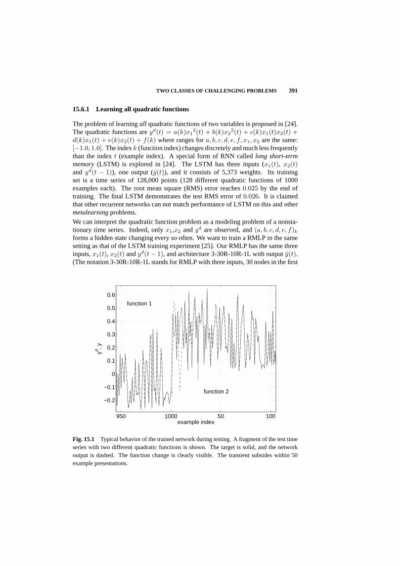
TWO CLASSES OF CHALLENGING PROBLEMS 391
15.6.1 Learning all quadratic functions
The problem of learningall quadratic functions of two variables is proposed in [24].The quadratic functions areyd(t) = a(k)x1
2(t) + b(k)x22(t) + c(k)x1(t)x2(t) +
d(k)x1(t) + e(k)x2(t) + f(k) where ranges fora, b, c, d, e, f, x1, x2 are the same:[−1.0, 1.0]. The indexk (function index) changes discretely and much less frequentlythan the indext (example index). A special form of RNN calledlong short-termmemory(LSTM) is explored in [24]. The LSTM has three inputs (x1(t), x2(t)and yd(t − 1)), one output (y(t)), and it consists of 5,373 weights. Its trainingset is a time series of 128,000 points (128 different quadratic functions of 1000examples each). The root mean square (RMS) error reaches0.025 by the end oftraining. The final LSTM demonstrates the test RMS error of0.026. It is claimedthat other recurrent networks can not match performance of LSTM on this and othermetalearningproblems.
We can interpret the quadratic function problem as a modeling problem of a nonsta-tionary time series. Indeed, onlyx1,x2 andyd are observed, and(a, b, c, d, e, f)k
forms a hidden state changing every so often. We want to train a RMLP in the samesetting as that of the LSTM training experiment [25]. Our RMLP has the same threeinputs,x1(t), x2(t) andyd(t− 1), and architecture 3-30R-10R-1L with outputy(t).(The notation 3-30R-10R-1L stands for RMLP with three inputs, 30 nodes in the first
950 1000 50 100
−0.2
−0.1
0
0.1
0.2
0.3
0.4
0.5
0.6
example index
yd , y
function 1
function 2
Fig. 15.1 Typical behavior of the trained network during testing. A fragment of the test timeseries with two different quadratic functions is shown. The target is solid, and the networkoutput is dashed. The function change is clearly visible. The transient subsides within 50example presentations.
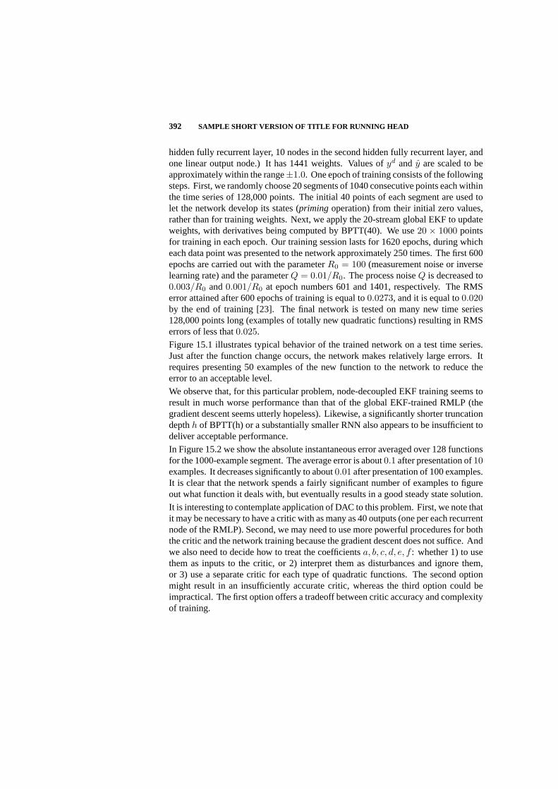
392 SAMPLE SHORT VERSION OF TITLE FOR RUNNING HEAD
hidden fully recurrent layer, 10 nodes in the second hidden fully recurrent layer, andone linear output node.) It has 1441 weights. Values ofyd and y are scaled to beapproximately within the range±1.0. One epoch of training consists of the followingsteps. First, we randomly choose 20 segments of 1040 consecutive points each withinthe time series of 128,000 points. The initial 40 points of each segment are used tolet the network develop its states (priming operation) from their initial zero values,rather than for training weights. Next, we apply the 20-stream global EKF to updateweights, with derivatives being computed by BPTT(40). We use20 × 1000 pointsfor training in each epoch. Our training session lasts for 1620 epochs, during whicheach data point was presented to the network approximately 250 times. The first 600epochs are carried out with the parameterR0 = 100 (measurement noise or inverselearning rate) and the parameterQ = 0.01/R0. The process noiseQ is decreased to0.003/R0 and0.001/R0 at epoch numbers 601 and 1401, respectively. The RMSerror attained after 600 epochs of training is equal to0.0273, and it is equal to0.020by the end of training [23]. The final network is tested on many new time series128,000 points long (examples of totally new quadratic functions) resulting in RMSerrors of less that0.025.
Figure 15.1 illustrates typical behavior of the trained network on a test time series.Just after the function change occurs, the network makes relatively large errors. Itrequires presenting 50 examples of the new function to the network to reduce theerror to an acceptable level.
We observe that, for this particular problem, node-decoupled EKF training seems toresult in much worse performance than that of the global EKF-trained RMLP (thegradient descent seems utterly hopeless). Likewise, a significantly shorter truncationdepthh of BPTT(h) or a substantially smaller RNN also appears to be insufficient todeliver acceptable performance.
In Figure 15.2 we show the absolute instantaneous error averaged over 128 functionsfor the 1000-example segment. The average error is about0.1 after presentation of10examples. It decreases significantly to about0.01 after presentation of 100 examples.It is clear that the network spends a fairly significant number of examples to figureout what function it deals with, but eventually results in a good steady state solution.
It is interesting to contemplate application of DAC to this problem. First, we note thatit may be necessary to have a critic with as many as 40 outputs (one per each recurrentnode of the RMLP). Second, we may need to use more powerful procedures for boththe critic and the network training because the gradient descent does not suffice. Andwe also need to decide how to treat the coefficientsa, b, c, d, e, f : whether 1) to usethem as inputs to the critic, or 2) interpret them as disturbances and ignore them,or 3) use a separate critic for each type of quadratic functions. The second optionmight result in an insufficiently accurate critic, whereas the third option could beimpractical. The first option offers a tradeoff between critic accuracy and complexityof training.
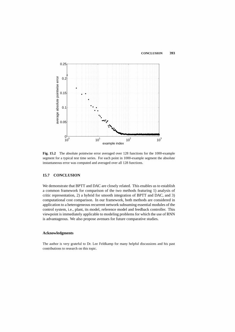
CONCLUSION 393
100
101
102
103
0
0.05
0.1
0.15
0.2
0.25
example index
aver
age
abso
lute
poi
ntw
ise
erro
r
Fig. 15.2 The absolute pointwise error averaged over 128 functions for the 1000-examplesegment for a typical test time series. For each point in 1000-example segment the absoluteinstantaneous error was computed and averaged over all 128 functions.
15.7 CONCLUSION
We demonstrate that BPTT and DAC are closely related. This enables us to establisha common framework for comparison of the two methods featuring 1) analysis ofcritic representation, 2) a hybrid for smooth integration of BPTT and DAC, and 3)computational cost comparison. In our framework, both methods are considered inapplication to a heterogeneous recurrent network subsuming essential modules of thecontrol system, i.e., plant, its model, reference model and feedback controller. Thisviewpoint is immediately applicable to modeling problems for which the use of RNNis advantageous. We also propose avenues for future comparative studies.
Acknowledgments
The author is very grateful to Dr. Lee Feldkamp for many helpful discussions and his pastcontributions to research on this topic.

Bibliography
1. P. J. Werbos. “Backpropagation through time: What it does and how to do it,”Proceedings of the IEEE,vol. 78, no. 10, pp. 1550–1560, 1990.
2. R. J. Williams and D. Zipser, “Gradient-based learning algorithms for recur-rent networks and their computational complexity,” in Chauvin and Rumelhart(Eds.),Backpropagation: Theory, Architectures and Applications,New York: L.Erlbaum and Associates, pp. 433–486, 1995.
3. P. J. Werbos, “Approximate dynamic programming for real-time control andneural modeling,”Handbook of Intelligent Control: Neural, Fuzzy and AdaptiveApproaches,D. A. White and D. A. Sofge, Eds., pp. 493–525, 1992.
4. D. V. Prokhorov, Adaptive Critic Designs and their Applications. Ph.D. disser-tation, Department of Electrical Engineering, Texas Tech University, Lubbock,TX, October 1997.
5. D. V. Prokhorov and D. C. Wunsch, “Adaptive Critic Designs,”IEEE Trans.Neural Networks,vol. 8, no. 5, pp. 997–1007, 1997.
6. D. V. Prokhorov, “Optimal Neurocontrollers for Discretized Distributed Param-eter Systems,”Proceedings of the American Control Conference,Denver, CO,2003, pp. 549–554.
7. L. A. Feldkamp and D. V. Prokhorov, “Observations on the Practical Use ofAdaptive Critics,”Proceedings of the 1997 IEEE SMC Conference,Orlando, FL,1997, pp. 3061–3066.
8. K. S. Narendra and A. M. Annaswamy,Stable Adaptive Systems,Prentice Hall,1989.
9. D. V. Prokhorov and L. A. Feldkamp, “Primitive Adaptive Critics,”Proceedingsof the 1997 IEEE International Conference on Neural Networks,Houston, TX,1997, pp. IV-2263–2267.
10. E. A. Wan, “Temporal Backpropagation for FIR neural networks,”Proceedingsof the 1990 International Joint Conference on Neural Networks,San Diego,1990, pp. I-575–580.
394
BIBLIOGRAPHY 395
11. L. A. Feldkamp and D. V. Prokhorov, “Phased Backpropagation: A Hybrid ofTB and BPTT,”Proceedings of the International Joint Conference on NeuralNetworks,Anchorage, AK, 1998, pp. 2262–2267.
12. L. A. Feldkamp, D. V. Prokhorov, C. F. Eagen, and F. Yuan, “Enhanced multi-stream Kalman filter training for recurrent networks,” in J. Suykens and J. Vande-walle (eds),Nonlinear Modeling: Advanced Black-Box Techniques,pp. 29–53.Kluwer Academic Publishers, 1998.
13. L. A. Feldkamp and G. V. Puskorius, “A signal processing framework based ondynamic neural networks with application to problems in adaptation, filteringand classification,”Proceedings of the IEEE,vol. 86, no. 11, pp. 2259–2277,1998.
14. L. A. Feldkamp, G. V. Puskorius, and D. V. Prokhorov, “Unified Formulation forTraining Recurrent Networks with Derivative Adaptive Critics,”Proceedings ofthe 1997 International Conference on Neural Networks,Houston, TX, 1997, pp.IV-2268–2272.
15. G. Lendaris and C. Paintz, “Training Strategies for Critic and Action NeuralNets in Dual Heuristic Programming Method,”Proceedings of InternationalConference on Neural Networks,Houston, TX, June, 1997, pp. 712–717.
16. G. Lendaris, T. T. Shannon, and A. Rustan, “A Comparison of Training Algo-rithms for DHP Adaptive Critic Neuro-control,”Proceedings of InternationalConference on Neural Networks (IJCNN’99),Washington,DC, July, 1999.
17. E. S. Plumer, “Optimal Control of Terminal Processes Using Neural Networks,”IEEE Trans. Neural Networks,Vol. 7, No. 2, 1996, pp. 408–418.
18. R. Stengel,Optimal Control and Estimation,Dover, 1994.
19. S. W. Piche, “Steepest Descent Algorithms for Neural Network Controllers andFilters,” IEEE Trans. Neural Networks,Vol. 5, No. 2, 1994, pp. 198–212.
20. Nonlinear Model Predictive Control,F. Allgower and A. Zheng (Eds.), Progressin systems and Control Theory Series, Vol. 26, Birkhauser Verlag, Basel 2000.
21. D. V. Prokhorov and L. A. Feldkamp, “Analyzing for Lyapunov Stability withAdaptive Critics,”Proceedings of the 1998 IEEE Conference on Systems, Man,and Cybernetics,San Diego, CA, 1998, pp. 1658–1661.
22. L. A. Feldkamp, T. M. Feldkamp, and D. V. Prokhorov, “Recurrent NeuralNetwork Training by nprKF Joint Estimation,”Proceedings of InternationalJoint Conference on Neural Networks ’02,Hawaii, 2002.
23. D. Prokhorov, L. Feldkamp, and I. Tyukin, “Adaptive Behavior with FixedWeights in RNN: Overview,”Proceedings of International Joint Conference onNeural Networks ’02,Hawaii, 2002.

396 BIBLIOGRAPHY
24. S. Younger, S. Hochreiter, and P. Conwell, “Meta-Learning with Backpropa-gation,” Proc. of the International Joint Conference on Neural Networks,pp.2001-2006, 2001.
25. S. Hochreiter, S. Younger, and P. Conwell, “Learning to Learn Using GradientDescent,”Proc. of ICANN,pp. 87-94, 2001.
26. L. A. Feldkamp and G. V. Puskorius, “Fixed weight controller for multiplesystems,”Proceedings of the 1997 International Joint Conference on NeuralNetworks,Houston TX, 1997, vol. II, pp. 773–778.
27. L. A. Feldkamp, G. V. Puskorius, and P. C. Moore, “Adaptive behavior fromfixed weight networks,”Information Sciences,vol. 98, pp. 217–235, 1997.
28. L. Feldkamp, D. Prokhorov, and T. Feldkamp, “Simple and Conditioned Adap-tive Behavior from Kalman Filter Trained Recurrent Neural Network,”NeuralNetworks,vol. 16, pp. 683–689, 2003.
29. D. V. Prokhorov, G. V. Puskorius, and L. A. Feldkamp, “Dynamical NeuralNetworks for Control,”A Field Guide to Dynamical Recurrent Networks,J.Kolen and S. Kremer (Eds.), IEEE Press, 2001, pp. 257–289.
30. D. V. Prokhorov, R. A. Santiago, and D. C. Wunsch, “Adaptive Critic Designs:A Case Study For Neurocontrol,”Neural Networks,vol. 8, no. 9, pp. 1367–1372,1995.
31. S. N. Balakrishnan and V. Biega, “Adaptive Critic Based Neural Networks forAircraft Optimal Control,”Journal of Guidance, Control and Dynamics,Vol. 19,No. 4, pp. 893–898, 1996.
32. G. K. Venayagamoorthy, R. G. Harley, and D. C. Wunsch, “Comparison ofHeuristic Dynamic Programming and Dual Heuristic Programming AdaptiveCritics for Neurocontrol of a Turbogenerator,”IEEE Trans. Neural Networks,vol. 13, no. 3, pp. 764–773, 2002.
33. P. H. Eaton, D. V. Prokhorov, and D. C. Wunsch, “Neurocontroller Alternativesfor “Fuzzy” Ball-and-Beam Systems with Nonuniform Nonlinear Friction,”IEEETrans. Neural Networks,vol. 11, no. 2, pp. 423–435, 2000.

Part III
Applications

16 Near-Optimal Control ThroughReinforcement Learning andHybridization
AUGUSTINE O. ESOGBUE and WARREN E. HEARNES II
Georgia Institute of Technology
Editor’s Summary: This chapter focuses on learning to act in a near-optimal man-ner through reinforcement learning for problems that either have no model or whosemodel is very complex. The emphasis here is on continuous action space (CAS)methods. Monte-Carlo approaches are employed to estimate function values in aniterative, incremental procedure. Derivative-free line search methods are used to finda near-optimal action in the continuous action space for a discrete subset of the statespace. This near-optimal policy is then extended to the entire continuous state spaceusing a fuzzy additive model. To compensate for approximation errors, a modifiedprocedure for perturbing the generated control policy is developed. Convergence re-sults, under moderate assumptions and stopping criteria, are established. Referencesto sucessful applications of the controller are provided.
16.1 INTRODUCTION
As real-world control problems become more complex, the application of traditionalanalytical and statistical control techniques requiring mathematical models of theplant becomes less appealing and appropriate. These methods assume that the systemto be controlled can be modeled correctly and precisely. Clearly, the accuracy of amodel affects the validity of the derived control policy. In many cases, the assumptionof certainty in the models is made not necessarily for validity, but for the need toobtain simpler and more readily solvable formulations.
When a model of the system is known, traditional well-developed theories such asoptimal control or adaptive control may be appropriate. Without a model however,these methods may not be adequate. In such situations, a model-free approach isrequired. Several approaches to model-free control exist. These include neural
399

400 NEAR-OPTIMAL CONTROL VIA REINFORCEMENT LEARNING
networks, fuzzy logic, and reinforcement learning. Model-free techniques learnthe control policy through either supervised or unsupervised means [37, 29, 38].Supervised learning, on the other hand, requires some sort of teacher to provide thedesired response at each time period. However, a teacher or expert may not always beavailable. Consequently, model-free control methods that can learn a control policyfor a complex system through online experience have been proposed [3, 4, 17, 25, 31].These are generally classified as reinforcement learning algorithms.
Model-free reinforcement learning methods are increasingly being used as potentand capable learning algorithms in intelligent autonomous systems for various ap-plications in fields such as control theory, optimization, and computer science. Anumber of successful applications of model-free reinforcement learning controllershave been demonstrated. Illustrative examples include [3, 4, 17, 21, 31, 34, 35].
Complex control processes are often characterized by inherent uncertainties in be-havior or measurement. An intelligent control algorithm for such processes mustdeal explicitly with these uncertainties. Practical applications that may introduceproblems better suited for model-free intelligent control include those with severenonlinearities, time-varying or unknown dynamics, partially observable states, orother complexities. These prevent the direct use of standard control techniques ofvariational calculus, classical dynamic programming, or global optimization.
The intelligent controller discussed in this chapter, an extension of the ContinuousAction Space (CAS) controller first proposed in [16] and developed further in [23],involves a hybrid approach that combines some of the advantages of reinforcementlearning, fuzzy sets, dynamic programming methods, neural networks, and nonlinearoptimization. The result is a hybrid algorithm that intelligently searches continuousaction spaces, learns a near-optimal control policy for continuous state spaces, anduses heuristic methods to dynamically allocate nodes during the learning phase.
16.2 TERMINAL CONTROL PROCESSES
The focus of this chapter is on closed-loop terminal control processes. In certainterminal control processes, the performance or objective function is not measuredfor a fixed time interval[0, T ]. Rather, the termination of the control process maydepend on the state. More specifically, a set of terminal states,ST, is defined. Thisset is the set-theoretic union of all successful termination states,S+, and all failuretermination states,S−:
ST = S+ ∪ S−. (16.1)
The control process then terminates when either a success or a failure state is reached.In general, terminal control problems are generally easier to solve using dynamicprogramming rather than classical control methods [6]. Throughout this chapter, itis instructive to assume that the system in question isset-point controllable. In otherwords, in a deterministic system there exists an action sequencea(1), . . . ,a(k−1)of admissible control actions for each initial states(1) ∈ S that drives the system

TERMINAL CONTROL PROCESSES 401
from s(1) to a successful termination states(k) ∈ S+ in finite time. Analogously,for systems with random disturbances, there exists an action sequence that drivesany initial state to a successful termination state with some positive probability. Thisensures that at least one control policy exists that will drive the system from any giveninitial state to a successful termination state or set-point.
In set-point regulation problems, a goal state or set-point,s?, is usually defined. Theobjective then, is to drive the system from any initial states ∈ S to the set-points? in an optimal manner with respect to some defined scalar return function. Someclassical measures, for such systems, include long-run expected reward with respectto external reinforcement signals, settling time or rise time with regard to transientresponse, or integral of absolute error (IAE) with regard to performance indices. Anumber of practical control systems, such as a manipulator for robot arms on thespace shuttle, an inverted pendulum on a movable cart, or a gain scheduler to reduceoscillations in power generators, can be formulated as set-point regulator problems.
Consider a possibly stochastic dynamical system with scalar returns. The set of allpossible states is represented by the setS while the set of all possible actions isrepresented byA. Them-dimensional state of the system at any time stepk is them-vectors(k) ∈ S and then-dimensional action taken at time stepk is then-vectora(k) ∈ A. The new states(k + 1) is defined by the transition functionτ :
s(k + 1) = τ (s(k),a(k), ω(k)) (16.2)
wherek = 0, 1, . . . andω(k) is some random disturbance. For ease of exposition,represent the probability thats(k + 1) = j whens(k) = i anda(k) = a aspij(a).It is further assumed that the transition functionτ for the process is not known a prioriand thatn = 1. This investigation is restricted to policies that are time-invariant. Forany given control policyπ : S 7→ A, the objective function for an infinite horizoncontrol problem can be defined [6, 5, 7] as
Vπ(s) = Eπ
[ ∞∑
k=0
γkR(s(k),a(k))|s(0) = s
]∀s ∈ S (16.3)
and letV (s) = infπVπ(s) ∀s ∈ S (16.4)
whereγ ∈ [0, 1) is a discount factor andEπ is the conditional expectation usingpolicy π. Vπ(s) represents the expected discounted total return using policyπ andstarting in states. A policy π? is γ-optimal if
Vπ?(s) = V (s) ∀s ∈ S. (16.5)

402 NEAR-OPTIMAL CONTROL VIA REINFORCEMENT LEARNING
Formulating the optimal control problem, as a dynamic program, results in thefollowing functional equation:
V (s) = infa∈A
[R(s,a) + γ
∑
s′∈S
pss′(a)V (s′)
]∀s ∈ S (16.6)
which represents the minimum expected discounted return when starting in statesand always following an optimal policy.
The following assumptions are made:
Assumption 16.2.1The return,R(s,a), for actiona taken in states is determinedimmediately or in some fixed time interval. Further,R(s,a) is bounded from belowby 0 and above by some numberB.
Assumption 16.2.2The system is set-point controllable. Furthermore, there existsa policyπ such thatVπ(s) < ∞ for all s ∈ S.
Assumption 16.2.3Multiple trials can be run on the system.
Approximate dynamic programming methods rely on repeated experimental runs.Systems must be allowed to experience both success–reaching a state inS+–andfailure–reaching a state inS−–without damaging the plant.
Assumption 16.2.4The transition functionτ(s,a, ω) is not known. Consequently,the transition probability,pss′(a), from states to states′ when actiona is taken isnot known.
16.3 A HYBRIDIZATION: THE GCS- ∆ CONTROLLER
Several issues make the current traditional and intelligent methods for controlling set-point regulation processes inadequate for some complex systems. Many processesand operations involve systems that are highly nonlinear, have a large number ofinteracting variables, or much of what is known about their modeling and controlis either imprecise or expressible mostly in linguistic terms. The model of theplant is either not known with certainty or cannot be easily solved. For example,the tethered satellite system retrieval problem has some very complex models, allof which are coarse approximations since including all parameters governing thephysical movements of a satellite on a tether is far too complex [13]. Yet, evenwith an approximate model the solution method is very cumbersome. Therefore, acontrol method that is not based on knowledge of the plant dynamics can theoreticallyprovide solutions in cases where traditional methods fail. In practical applications,such as the tethered satellite retrieval problem, failures are costly and prohibitive.Simulations of the plant can help jump-start the learning process in these cases.
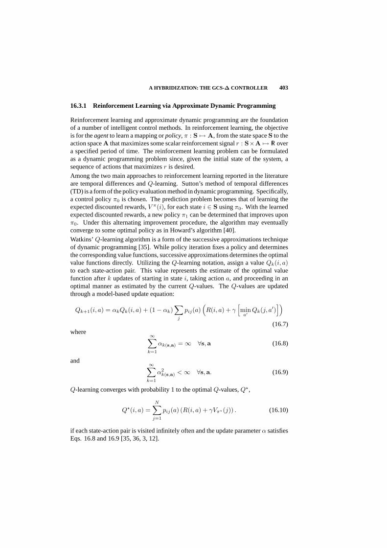
A HYBRIDIZATION: THE GCS- ∆ CONTROLLER 403
16.3.1 Reinforcement Learning via Approximate Dynamic Programming
Reinforcement learning and approximate dynamic programming are the foundationof a number of intelligent control methods. In reinforcement learning, the objectiveis for theagentto learn a mapping orpolicy, π : S 7→ A, from the state spaceS to theaction spaceA that maximizes some scalar reinforcement signalr : S×A 7→ R overa specified period of time. The reinforcement learning problem can be formulatedas a dynamic programming problem since, given the initial state of the system, asequence of actions that maximizesr is desired.
Among the two main approaches to reinforcement learning reported in the literatureare temporal differences andQ-learning. Sutton’s method of temporal differences(TD) is a form of the policy evaluation method in dynamic programming. Specifically,a control policyπ0 is chosen. The prediction problem becomes that of learning theexpected discounted rewards,V π(i), for each statei ∈ S usingπ0. With the learnedexpected discounted rewards, a new policyπ1 can be determined that improves uponπ0. Under this alternating improvement procedure, the algorithm may eventuallyconverge to some optimal policy as in Howard’s algorithm [40].
Watkins’Q-learning algorithm is a form of the successive approximations techniqueof dynamic programming [35]. While policy iteration fixes a policy and determinesthe corresponding value functions, successive approximations determines the optimalvalue functions directly. Utilizing theQ-learning notation, assign a valueQk(i, a)to each state-action pair. This value represents the estimate of the optimal valuefunction afterk updates of starting in statei, taking actiona, and proceeding in anoptimal manner as estimated by the currentQ-values. TheQ-values are updatedthrough a model-based update equation:
Qk+1(i, a) = αkQk(i, a) + (1− αk)∑
j
pij(a)(R(i, a) + γ
[min
a′Qk(j, a′)
])
(16.7)where ∞∑
k=1
αk(s,a) = ∞ ∀s,a (16.8)
and ∞∑
k=1
α2k(s,a) < ∞ ∀s,a. (16.9)
Q-learning converges with probability 1 to the optimalQ-values,Q?,
Q?(i, a) =N∑
j=1
pij(a) (R(i, a) + γVπ?(j)) . (16.10)
if each state-action pair is visited infinitely often and the update parameterα satisfiesEqs. 16.8 and 16.9 [35, 36, 3, 12].

404 NEAR-OPTIMAL CONTROL VIA REINFORCEMENT LEARNING
Watkins’Q-learning has been modified by a number of researchers. Berenji [10]forexample, proposed an extension ofQ-learning into fuzzy environments and termedit Fuzzy Q-learning. This has the advantage of improvements in the learning ratebut has the disadvantage of requiring some initial rulebase. Similarly, Oh, et al.,[32] developed an approach that initializes the conventionalQ-values withQ-valuesderived from a fuzzy rulebase. With a better initial starting point, theQ-learningalgorithm reinforced with a beneficial knowledge base and intelligence, may take lesstime to converge to the optimalQ-values. Wiering and Schmidhuber [39] modifyPeng and WilliamsQ(λ) procedure [33] by allowingQ-value updates to be postponeduntil they are needed. By doing this "lazy learning" process, the complexity of thelookup table is bounded by the number of actions instead of the number of state-actionpairs.
Several methods utilize a hybrid approach to control in order to take advantage ofthe separate strengths of each method such as neural networks, fuzzy control, andreinforcement learning to compensate for the weaknesses of the others. Berenjiextended his own Generalized Approximate Reasoning-based Intelligent Control(GARIC) model by using a set of intelligent agents controlled, at the top level, byFuzzyQ-learning and, at the local level, by the GARIC architecture [10]. Takingthe modifications one step further, Berenji and Sarar [11], allow collaboration amongthese intelligent agents for a specified period of time in their MULTI-GARIC-Qmethod. A critic, or action evaluator, then chooses the agent that has learned the"best" control policy to determine which agent ultimately controls the system. On adifferent tangent, Kandadai and Tein modify Berenji’s original GARIC architecture[26]. Realizing that a disadvantage to the GARIC model is the assumption of anexisting linguistic rulebase, Kandadai and Tien use a supervised learning schemeusing both reinforcement learning and backpropagation to generate this linguisticrulebase. The result is a fuzzy-neural system that can generate its own control policythrough reinforcements.
The foundation for the theory of the Statistical Fuzzy Associative Learning Con-troller (SFAL-C), introduced in 1993 by Esogbue and Murrell [17], was developedextensively in [31]. The SFAL-C is a hybrid fuzzy controller and neural networkwith a dynamic programming like optimizer. A variation of temporal differences isused to estimate the long-run reward for choosing a specific reference action in eachstate. After the learning process has ended, the long-run reward estimates for eachaction are transformed into a fuzzy set membership function for the proper action atthat particular state. Fuzzy inference is used to generalize these learned controls tothe entire state space [19, 17, 18, 15, 21]. Additional properties of this controllerare provided in [14]. The successful operation of the fuzzy adaptive controller wasdemonstrated on several environments.
16.3.2 Review of CAS Controller
The controller which forms the focal attention of this chapter is an extension ofthe Continuous Action Space (CAS) algorithm proposed in [16, 23]. To motivate

A HYBRIDIZATION: THE GCS- ∆ CONTROLLER 405
the current work, it is instructive to first present a brief outline of the structure andproperties of this algorithm. The CAS algorithm usesQ-learning as the evaluatorfor a discrete subset of actions for continuous action space control. It begins with arepresentative finite discrete subsetaj , j = 1, . . . , A, for each statei, spanning someinterval of uncertainty (IoU) regarding the location of the optimal control action in thecontinuous action spaceA. TheQ-learning algorithm determines the optimal policyusing only this action subset. Based on the optimal policy using only actions in therepresentative discrete subsetaj , the interval of uncertainty regarding the locationof the optimal action can be reduced for selected states. For the new interval ofuncertainty, the locations of the reference actions are adjusted and theQ-values arere-evaluated. As the CAS algorithm continues, the intervals of uncertainty for eachstate are reduced toward 0, centering on the optimal action in the continuous actionspace if certain assumptions are maintained. The choice of the reduction parameterβ,learning rateα, thresholdN , and initialQ-valueM all affect the rate of convergence.
The key to the efficiency of the CAS algorithm is that the optimal policy can, inmany cases, be determined before theQ-learning algorithm converges to the optimalfunctional values. For example, consider a discrete approximation to the invertedpendulum balancing problem [2]. With the objective to minimize the discountedsum of the squared error from the set-point, one discretization of the state space mayconsist of51 × 5 × 51 × 5 discrete states forθ, ∆θ, x, and∆x, respectively. EachQn(i, a) value is arbitrarily initialized at some large integer. Using a full backupfor each iteration, 3401 iterations are necessary before theQ-values converge towithin ε = 0.0001 of the optimal functional values. Yet, the algorithm determinesthe optimal policy after only 36 iterations, as shown in Figure 16.1 which plots thesepolicy changes during the 3401 iterations, a 98.94% reduction in the computationaleffort. Detailed investigation of possible computational savings is reported in [16, 23].Basing the policy improvement procedure on the learned optimal policy at the earlierstages, before the optimal value is learned, is equivalent to waiting for theQ-learningalgorithm to converge.
In the problems of interest in this chapter, the action spaceA is not discrete but con-tinuous over a compact interval ofR. Each discrete statei (defined by a discretizationof the continuous state space into a subset of regions that serve as an approximationto the continuous state space) has an interval of uncertainty (IoU) which contains thetrue optimal actionπ?(i). In the CAS algorithm, the estimates of theQ(i,aj) valuesfor each statei serve as a guide for reducing the interval of uncertainty. Initially, thisinterval is the entire action spaceA. Each reduction is by a factor of0 < β < 1.Therefore, the interval can be made arbitrarily small using successive reductions. Letthe reference action subset for statei be defined
AA(i) = a1,a2, . . . ,aA ⊂ A. (16.11)
Further, define the transformation
B(β,AA(i), k) = β[a1 − aj? ] + aj? , . . . , β[aA − aj? ] + aj? (16.12)

406 NEAR-OPTIMAL CONTROL VIA REINFORCEMENT LEARNING
Fig. 16.1 Optimal policy is found in considerably fewer iterations than the optimal functionalvalues in an inverted pendulum balancing example.
wherej? = argminjQk(i,aj) (16.13)
as the Successive Reduction procedure. If the initial interval of uncertainty,IoU0, isdenoted as
IoU0 = supaa ∈ A − inf
aa ∈ A, (16.14)
then it requires at leastln ε− ln IoU0
ln β(16.15)
successive reductions of the interval of uncertainty to reach any specified accuracyε > 0.
There is a positive probability, however small, that the optimal action on the referencesubsetaj will not be the basis for the successive reduction. This implies that thereis a positive probability that the optimal action on the reference subset will not becontained in the interval of uncertainty for the next iteration of the CAS algorithm.
Consider the sequence of estimatesQ0(i, a), Q1(i, a), . . . , Q′k(i, a) for some state-
action pairi, a. Since the true optimalQ-value,Q(i, a) is not known, one possiblemeasure of the quality of the estimation is the mean and sample variance of the lastn estimates. Define
Q′k(i, a) ≡∑k′
k=k′−n+1 Qk(i, a)n
∀i, a (16.16)

A HYBRIDIZATION: THE GCS- ∆ CONTROLLER 407
and
s2Q′k(i,a) ≡
∑k′
k=k′−n+1(Qk(i, a)− Q′k(i, a))2
n− 1∀i, a. (16.17)
By appropriately choosing statistical hypotheses and a level of significance, the Suc-cessive Reduction procedure could be modified such that the interval of uncertaintyregarding the optimal action would not eliminate any reference action in the subsetaj that could not be shown to be statistically significantly non-optimal.
In general, the above modification results have one of the following two effects.Either the Successive Reduction Procedure would continue to reduce the intervalof uncertainty to an arbitrarily small interval, or, the interval of uncertainty wouldbecome fixed around some subset of actions which had estimatedQ-values such thattheir long-run performance was not statistically different. In the first case, the optimalaction is found by the reduction of the interval. In the second case, the optimal actionis not necessarily found, but the action determined is near-optimal. The theoreticalconvergence is guaranteed in deterministic systems by the appropriate choice of whichstates to first apply the successive reduction procedure. The constructed sequence,S1, . . ., SN , accomplishes this but, under Assumption 16.2.4, this classification ofstates cannot be made explicitly. Consequently, the suggested approach is to employheuristics that attempt to approximate these subsets ofS.
16.3.3 The GCS-∆ Controller
The CAS algorithm demonstrates the ability to efficiently learn anε-optimal controllaw for the inverted pendulum and power system stabilization problems, using heuris-tics to focus its search and eliminate some unnecessary computations [16]. In thissection, we extend the controller, with some additional enhancements, to problemsinvolving approximating continuous state spaces using fuzzy sets.
The CAS algorithm is an efficient method for applying approximate dynamic pro-gramming methods to problems with continuous action spaces. To achieve a veryfine approximation to a continuous state space, many discrete states are needed andthe efficiency of the CAS algorithm deteriorates. A generalized continuous space(GCS) algorithm is proposed that uses fuzzy sets to generalize the learned informa-tion throughout the continuous state space. The GCS algorithm learns the propercontrol for each ofS reference statess1, . . . , sS with the CAS algorithm. Theselearned values ofQn(si,aj) for the discrete state space serve as the required expertknowledge to generate a rulebase. The state spaceS is partitioned into a set ofSfuzzy sets corresponding to the center of the discrete states in the CAS algorithm.A Gaussian membership functionµsi is defined for each fuzzy subsetsi of the statespace:
µsi(x) = exp(−‖x− si‖2∞/2σ2i ) i = 1, . . . , S (16.18)
wheresi is the center or prototype member of the fuzzy setsi, ‖ · ‖∞ is the supnorm, andσi defines its point of inflection. Denote the set ofS prototype members,s1, s2, . . . , sS, as the reference state spaceSS .
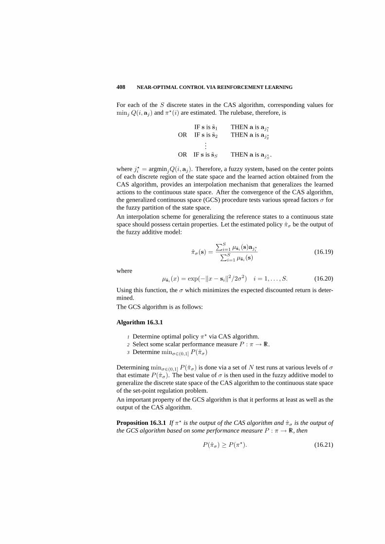
408 NEAR-OPTIMAL CONTROL VIA REINFORCEMENT LEARNING
For each of theS discrete states in the CAS algorithm, corresponding values forminj Q(i,aj) andπ?(i) are estimated. The rulebase, therefore, is
IF s is s1 THEN a is aj?1
OR IF s is s2 THEN a is aj?2
...OR IF s is sS THEN a is aj?
S.
wherej?i = argminjQ(i,aj). Therefore, a fuzzy system, based on the center points
of each discrete region of the state space and the learned action obtained from theCAS algorithm, provides an interpolation mechanism that generalizes the learnedactions to the continuous state space. After the convergence of the CAS algorithm,the generalized continuous space (GCS) procedure tests various spread factorsσ forthe fuzzy partition of the state space.
An interpolation scheme for generalizing the reference states to a continuous statespace should possess certain properties. Let the estimated policyπσ be the output ofthe fuzzy additive model:
πσ(s) =∑S
i=1 µsi(s)aj?i∑S
i=1 µsi(s)(16.19)
whereµsi(x) = exp(−‖x− si‖2/2σ2) i = 1, . . . , S. (16.20)
Using this function, theσ which minimizes the expected discounted return is deter-mined.
The GCS algorithm is as follows:
Algorithm 16.3.1
1 Determine optimal policyπ? via CAS algorithm.2 Select some scalar performance measureP : π → R.3 Determineminσ∈(0,1] P (πσ)
Determiningminσ∈(0,1] P (πσ) is done via a set ofN test runs at various levels ofσthat estimateP (πσ). The best value ofσ is then used in the fuzzy additive model togeneralize the discrete state space of the CAS algorithm to the continuous state spaceof the set-point regulation problem.
An important property of the GCS algorithm is that it performs at least as well as theoutput of the CAS algorithm.
Proposition 16.3.1 If π? is the output of the CAS algorithm andπσ is the output ofthe GCS algorithm based on some performance measureP : π → R, then
P (πσ) ≥ P (π?). (16.21)

A HYBRIDIZATION: THE GCS- ∆ CONTROLLER 409
Proof: The membership function value ofs in each fuzzy partition is
µsi(s) = exp(−‖s− si‖2/2σ2) i = 1, . . . , S. (16.22)
wheresi is the center of thei-th fuzzy partition. Consider any two fuzzy partitions,i andj. The distances froms to si andsj are‖s − si‖ and‖s − sj‖, respectively.Without loss of generality, let
‖s− si‖ ≥ ‖s− sj‖. (16.23)
Therefore,‖s− si‖ = ‖s− sj‖+ ε (16.24)
for someε ≥ 0. The membership ofs in fuzzy partitionsi is
µsi(s) = exp(−‖s− si‖2/2σ2)= exp(−(‖s− sj‖+ ε)2/2σ2)= exp(−(‖s− sj‖2 + 2‖s− sj‖ε + ε2)/2σ2)= µsj (s) exp(−(2‖s− sj‖ε + ε2)/2σ2).
(16.25)
As σ → 0+, exp(−(2‖s− sj‖ε + ε2)/2σ2) → 0 for any value ofε ≥ 0. Therefore,
limσ→0+
(µsi(s)a
?(i) + µsj (s)a?(j)
µsi(s) + µsj (s)
)→ a?(i). (16.26)
The argument can be extended to any finite number of fuzzy partitions with the sameresult. Therefore, for any performance measureP ,
limσ→0+
P (πσ) → P (π?), (16.27)
andP (πσ) 6< P (π?). 4
In this section, we wish to discuss an aspect of the CAS procedure relative to themaintenance of the integrity of its output. We note that the CAS algorithm learns anoptimal action for a particular discrete state. When fuzzy sets are used to generalizethis learned control law, an improper choice of fuzzy membership functions can resultin a defuzzified output that is different from the learned optimal action. Considerthe states such thatµs1(s) = 1. If the CAS algorithm determines thatπ?(1) = a?,then it is a desirable property thatπσ(s) = a?, also. With standard center-of-areadefuzzification procedure, if the value ofσ is chosen to be too large, it is likely thatthis is not true. A preliminary analysis into this phenomenon generates a range ofσwhere this property generally holds. Forπσ(si) ≈ π?(i) for statei, the followingmust hold:
µsj (si) ¿ 1 ∀j 6= i. (16.28)
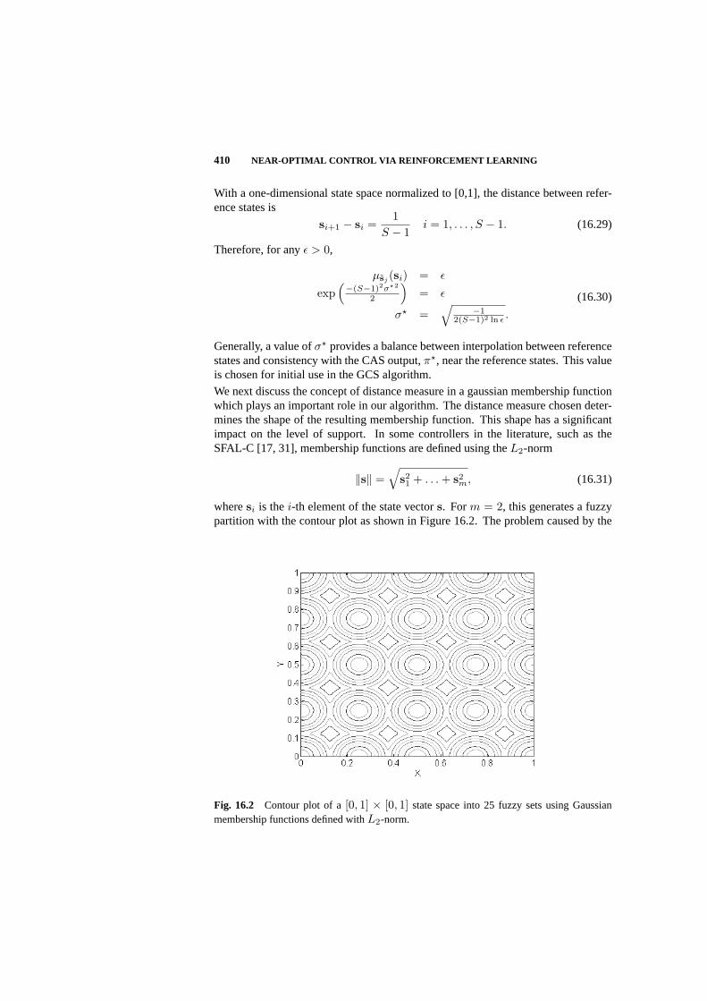
410 NEAR-OPTIMAL CONTROL VIA REINFORCEMENT LEARNING
With a one-dimensional state space normalized to [0,1], the distance between refer-ence states is
si+1 − si =1
S − 1i = 1, . . . , S − 1. (16.29)
Therefore, for anyε > 0,
µsj(si) = ε
exp(−(S−1)2σ?2
2
)= ε
σ? =√
−12(S−1)2 ln ε .
(16.30)
Generally, a value ofσ? provides a balance between interpolation between referencestates and consistency with the CAS output,π?, near the reference states. This valueis chosen for initial use in the GCS algorithm.
We next discuss the concept of distance measure in a gaussian membership functionwhich plays an important role in our algorithm. The distance measure chosen deter-mines the shape of the resulting membership function. This shape has a significantimpact on the level of support. In some controllers in the literature, such as theSFAL-C [17, 31], membership functions are defined using theL2-norm
‖s‖ =√
s21 + . . . + s2
m, (16.31)
wheresi is thei-th element of the state vectors. Form = 2, this generates a fuzzypartition with the contour plot as shown in Figure 16.2. The problem caused by the
Fig. 16.2 Contour plot of a[0, 1] × [0, 1] state space into 25 fuzzy sets using Gaussianmembership functions defined withL2-norm.

A HYBRIDIZATION: THE GCS- ∆ CONTROLLER 411
L2-norm in higher dimensions is the lack ofsupportfor a large portion of the statespace. Due to the negative exponential nature, the theoretical support of each fuzzystatesi is S. However, in practice, the support as the set of all statess ∈ S suchthatµsi(s) ≥ ε for someε > 0 should be considered. In practical applications offuzzy control, it has been empirically determined that an odd number of fuzzy setsis desired and that every states should be a member of one fuzzy partition to degree0.5:
maxi
µsi(s) ≥ 0.5 ∀s ∈ S. (16.32)
With membership functions defined by theL2-norm and a value ofσ defined as in(16.30), the radius of the support circle around eachsi that meets (16.32) is
r0.5 =1
(S)1m − 1
√ln 0.5ln ε
, (16.33)
wherem is the number of dimensions in the state vector andε is the one used todetermineσ in (16.30). With a uniform distribution ofsi, i = 1, . . . , 25 for m = 2,the total area that meets (16.32) is
[4 · 1
4+ 4 · 3 · 1
2+ 3 · 3
]πr2
0.5 = 16πr20.5 = 0.4729. (16.34)
Therefore, 52.71% of the state space is underrepresented by theL2-norm Gaussianmembership functions.
Defining the membership functions with theL∞-norm gives the fuzzy partitionsillustrated in Figure 16.3. TheL∞-norm for state vectors is defined as:
‖s‖∞ = sup|s1|, . . . , |sm| (16.35)
wheresi is the i-th element of the state vectors. Under this representation, thecontours for various levels of membership function values are rectangles instead ofcircles. Therefore, with a uniform distribution ofsi, i = 1, . . . , 25 for m = 2, thetotal area that meets (16.32) is
[4 · 1
4+ 4 · 3 · 1
2+ 3 · 3
]πr2
0.5 = 16(2r0.5)2 = 0.6021. (16.36)
Therefore, only 39.79% of the state space is underrepresented by theL∞-normGaussian membership functions. The difference is even more significant for lowervalues of desired representation. Consider the value ofα at the boundaries of thediscrete states used in the CAS algorithm:
rα =1
(S)1m − 1
= 0.125 (16.37)
whereα = ε
14 . (16.38)
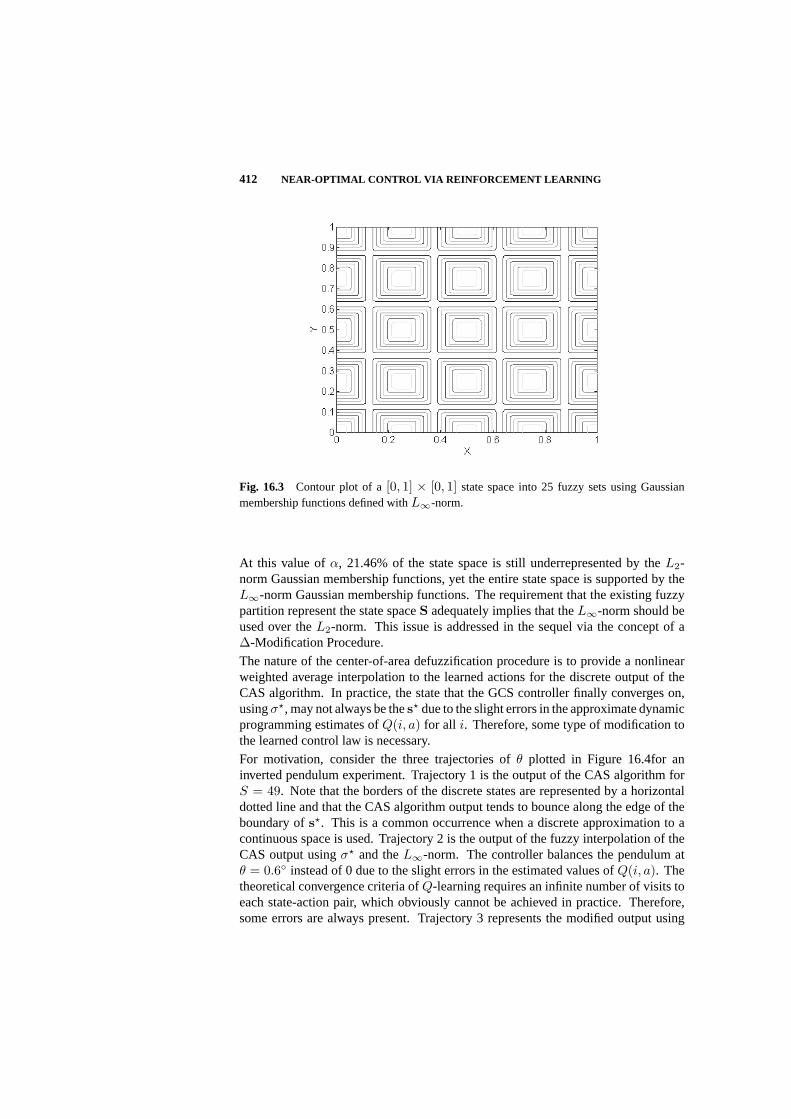
412 NEAR-OPTIMAL CONTROL VIA REINFORCEMENT LEARNING
Fig. 16.3 Contour plot of a[0, 1] × [0, 1] state space into 25 fuzzy sets using Gaussianmembership functions defined withL∞-norm.
At this value ofα, 21.46% of the state space is still underrepresented by theL2-norm Gaussian membership functions, yet the entire state space is supported by theL∞-norm Gaussian membership functions. The requirement that the existing fuzzypartition represent the state spaceS adequately implies that theL∞-norm should beused over theL2-norm. This issue is addressed in the sequel via the concept of a∆-Modification Procedure.
The nature of the center-of-area defuzzification procedure is to provide a nonlinearweighted average interpolation to the learned actions for the discrete output of theCAS algorithm. In practice, the state that the GCS controller finally converges on,usingσ?, may not always be thes? due to the slight errors in the approximate dynamicprogramming estimates ofQ(i, a) for all i. Therefore, some type of modification tothe learned control law is necessary.
For motivation, consider the three trajectories ofθ plotted in Figure 16.4for aninverted pendulum experiment. Trajectory 1 is the output of the CAS algorithm forS = 49. Note that the borders of the discrete states are represented by a horizontaldotted line and that the CAS algorithm output tends to bounce along the edge of theboundary ofs?. This is a common occurrence when a discrete approximation to acontinuous space is used. Trajectory 2 is the output of the fuzzy interpolation of theCAS output usingσ? and theL∞-norm. The controller balances the pendulum atθ = 0.6 instead of 0 due to the slight errors in the estimated values ofQ(i, a). Thetheoretical convergence criteria ofQ-learning requires an infinite number of visits toeach state-action pair, which obviously cannot be achieved in practice. Therefore,some errors are always present. Trajectory 3 represents the modified output using

A HYBRIDIZATION: THE GCS- ∆ CONTROLLER 413
the∆-modification procedure explained in detail below. This method ensures thatthe pendulum is balanced at approximately0.
Fig. 16.4 Trajectories ofθ for (1) the CAS algorithm, (2) the GCS algorithm, and (3) theGCS algorithm with∆-modification, all withS = 49.
The essence of the∆-modification is to determine an adjustment fuzzy state∆ withactiona∆ such that the modified control law
π∆(s) = π(s) + µ∆a∆ (16.39)
drives the system to the set-point. Assume that the CAS algorithm has delivereda policyπ? such that the system does not fail for each states during the test runs.Empirically, it has been determined that the center-of-area defuzzification withσ?
provides a response as shown in Trajectory 2 in Figure 16.4. During the first testrun, denote the final state at timeT usinga∆ = 0 ass(0, T ). This state defines thelocation of the prototype member of∆:
µ∆(s(0, T )) = 1 (16.40)
with σ = σ?. Choosing an initial valuea∆ = a ∈ A, a subsequent test run usingπ∆ provides the information necessary to update the estimate ofa∆. Formulatingthe problem as:
f(a∆) ≡ s(a∆, T )− s?, (16.41)
the secant algorithm may be used to determine the root of the functionf .
Algorithm 16.3.2
1 Input: Controller from GCS algorithm.

414 NEAR-OPTIMAL CONTROL VIA REINFORCEMENT LEARNING
2 Perform test run usingπ.3 c ← 04 ∆c ← s(0, T )5 a∆c
← a0
6 while s(a∆c , T ) 6= s? do7 Perform test run usingπ∆c
.8 ∆c+1 ← s(a∆c
, T )9 a∆c+1 ← a∆c − (∆c+1 − s?)(∆c+1 −∆c)/(a∆c+1 − a∆c)∆c
10 od
16.4 EXPERIMENTAL INVESTIGATION OF THE GCS- ∆ ALGORITHM
The experiments conducted in this section illustrate the GCS algorithm and identifythe effects of the∆ modification procedure on the performance measure SSE. Thefactors that may have an impact are the cardinality of discrete state space,|S| = S, thecardinality of reference action set,|AA| = A, and the number of expected iterations.A full factorial design of the23 experiment estimates the effect of the main effectsand small-order interactions on the computational savings for the 4-input/1-outputinverted pendulum balancing problem [2]. The problem is to learn to balance anupright pole that is attached by a pivot to a cart, while keeping the cart at the centerof the region it may move through. The discount factorγ was held constant at 0.99.The levels for each factor are given in Table 16.1. The performance improvements
Table 16.1 Levels of variables in full factorial experiment.
for each of the 8 runs are given in Table 16.2. Themean finalθ valueis defined as theaverage value ofθ over each of the 8 replications at 10.0 seconds in the test phase.The main effects and first order interaction are given in Table 16.3.
Each of the 8 replications of the 8 runs represents the application of the GCS-∆algorithm. Each of the three factors is at either a high (1) or a low (0) level. Fromthe performance improvements, an estimate of the effects and first-order interactionscan be made. A plot of the main effects is shown in Figure 16.5, plotting the threefactors: (1) State space cardinality, (2) Action space cardinality, (3) Number ofexpected iterations..
The experimental data provides several insights:
1. The average performance improvement in SSE of 58% is a significant improve-ment. The∆ modification procedure reduces the approximation error of theGCS algorithm in an effective manner. The additional computations required
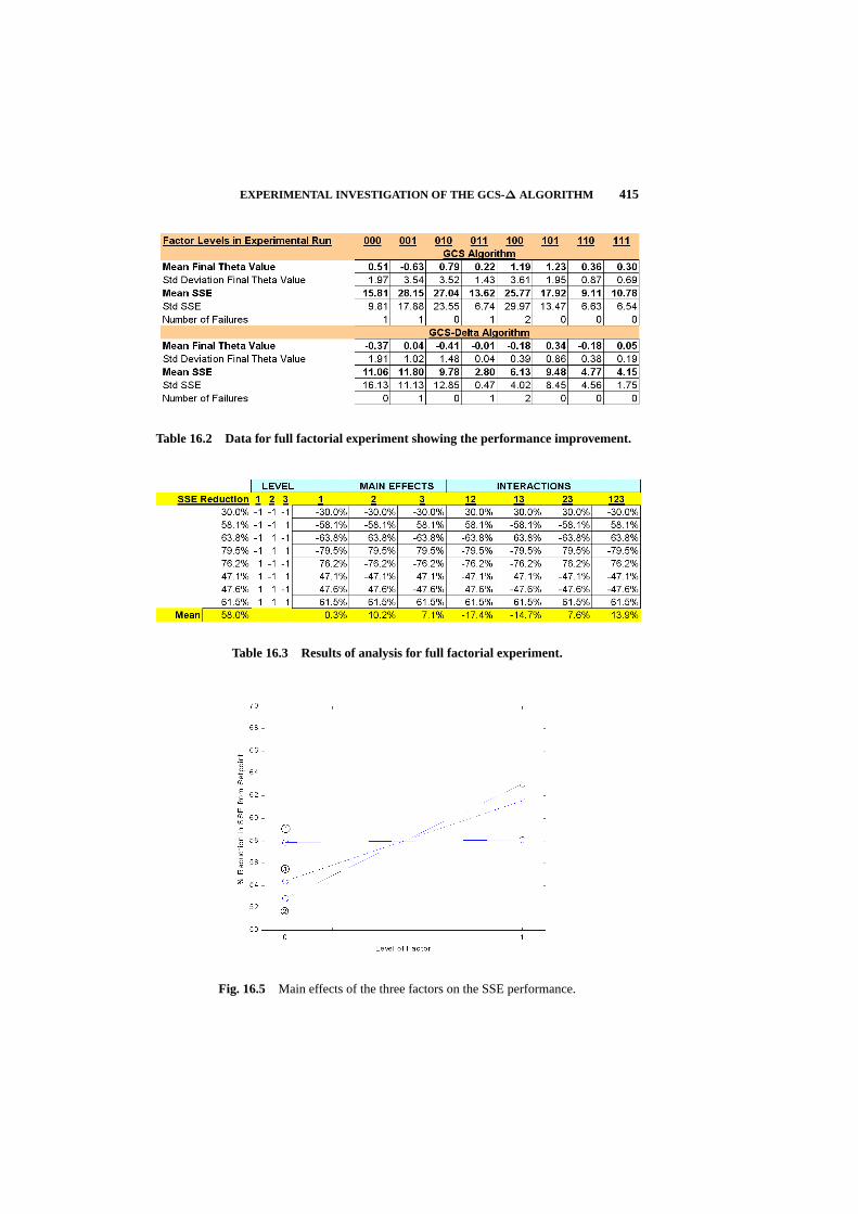
EXPERIMENTAL INVESTIGATION OF THE GCS- ∆ ALGORITHM 415
Table 16.2 Data for full factorial experiment showing the performance improvement.
Table 16.3 Results of analysis for full factorial experiment.
Fig. 16.5 Main effects of the three factors on the SSE performance.

416 NEAR-OPTIMAL CONTROL VIA REINFORCEMENT LEARNING
are minimal since the procedure works during the testing phase of the learnedcontrol policy.
2. Though the main effect of increasing the expected number of iterations ispositive, it does not guarantee improvement.
3. Similar to the GCS algorithm doing at least as well as the CAS, the GCS-∆algorithm, with its basis in both, will perform at least as well as either.
Figures 16.6 and 16.7 show a sample trajectory forθ using the GCS algorithmand the GCS-∆ algorithm, respectively. The approximation error in the resultingnear-optimal control policy is greatly reduced with the latter.
Fig. 16.6 Sample trajectory for the inverted pendulum balancing problem using the GCSalgorithm.
The CAS algorithm improves the performance of standardQ-learning by systemati-cally reducing the action space to some arbitrarily small interval. This insures that anε-optimal control policy is found under the strict quasi-convexity assumption. TheGCS algorithm determines the value of a spread parameter,σ, which best interpolatesthe discrete state space in the CAS algorithm to the continuous state space. However,due to approximation error, some correction may be required by the∆ modificationprocedure. The performance of the proposed algorithms has been illustrated with theinverted pendulum balancing problem.
16.5 DYNAMIC ALLOCATION OF CONTROLLER RESOURCES
A long-standing research question in dynamic programming is the allocation ofresources for problems of high dimension [7, 30]. As state and action dimensions are

DYNAMIC ALLOCATION OF CONTROLLER RESOURCES 417
Fig. 16.7 Sample trajectory for the inverted pendulum balancing problem using the GCS-∆algorithm.
increased, the resources used to approximate the state space and estimate the controlaction can increase exponentially. Fuzzy sets, through inference and defuzzification,can approximate any continuous function within anyε > 0 accuracy [27]. However,the number of rules and membership functions required to achieve this may beprohibitive. Similar to the curse of dimensionality in dynamic programming, thereexists a tradeoff in function approximation–as the number of nodes increase, theaccuracy of the approximation may also increase, but the efficiency of the learningalgorithm declines. This section presents a heuristic method to dynamically allocatenodes to the state space that achieve the desired approximation accuracy but does notburden the learning process in a prohibitive manner.
Additional state nodes require additional computations. Therefore, it is imperativeto use a minimal amount of resources to successfully attack the problem at hand.As motivation, during a typical learning phase of 100,000 time steps in a testbedproblem, the distribution of states visited in Figure 16.8 shows how little of the timeis spent in the regions far from the set-point of [0,0]. With the majority of the timespent in the set-point region, it is conjectured that refining the approximation in thatarea will improve the performance. This conjecture is supported by the experimentsin the sequel. Regions that are visited a disproportionately large number of times overthe course of the learning phase of the controller are likely to be important regionswhere a finer resolution is beneficial.
Several exploration strategies may be used inQ-learning to identify the optimal actionamong the subset of actions at each state. Regions of high visitation under a uniformexploration strategy may not accurately depict regions of high visitation under theoptimal control policy. To overcome this problem, the regions are determined using

418 NEAR-OPTIMAL CONTROL VIA REINFORCEMENT LEARNING
Fig. 16.8 Distribution of states visited during typical inverted pendulum learning phase.
the learned control policy. This is easily accomplished during the policy updatestage in the CAS algorithm. During that stage, the expected number of transitionsuntil the set-point is reached is already estimated under the CAS, GCS, and GCS-∆ algorithms. Under a successful learned control policyπ, it is expected that theregion containing the set-points? will be visited with a high relative frequency and,therefore, will be one of the discrete regions where additional nodes are allocated.
If all |S| = S states are visited equally often then each statesi, i = 1, . . . , S has arelative frequency of1/S. The notion of a “highly visited state” is defined in thischapter as one that has been the visited with a relative frequency greater thanp/S,wherep is some integer in1, . . . , S such as 3 or 5. Denote the subset of regions thatmeet the criteria for high visitation as
Ω = si | η(si) > p/S (16.42)
whereη(si) is a measure of the relative frequencysi has been visited andp/S ∈ (0, 1].The dynamic allocation of state nodes in the CAS algorithm is performed as outlinedin Algorithm 16.5.1.
Algorithm 16.5.1
1 Set boundary condition:V (s?) = 0.2 Initialize aj for all states.3 SetQ0(i,aj) = M À 0 ∀i, j.4 n(i) ← 0 ∀i5 while n(i) < N ∀i do6 Perform an iteration ofQ-learning.

CONCLUSIONS AND FUTURE RESEARCH 419
7 if Policy doesn’t change for statei8 n(i) ← n(i) + 19 else
10 n(i) ← 011 fi12 if Reduction criterion is met for statei13 Reduce IoU byβ < 1 aroundaj? , j? =argminjQn(i,aj) ∀i fi14 for each statesi do15 if η(si) > p/S16 Divide statesi into 3m sub-states.fi17 od
Experimental data on the effects of adding nodes in regions of high visitation on SSEfor the GCS-∆ algorithm provides the following insights [24]:
1. The average change in the SSE from using the standard uniform distribution ofstates to a distribution that clustered more states in regions of high visitation was-44.7%± 72.5%. The range contains 0 and no real effect can be interpreted.
2. The primary reason for the lack of visible improvement is that the GCS-∆algorithm directly reduces approximation error in the learned control policyfrom the CAS and GCS algorithms. Adding nodes in regions of high visitationimproves the output of the CAS, and therefore the GCS, algorithms but notnecessarily the GCS-∆. Other random factors are more significant.
3. The GCS-∆ algorithm can do no worse than the CAS and GCS algorithms,therefore even though there is no improvement, on the average, when addingthe nodes in regions of high visitation, there may be some improvement in aparticular instance.
Adding nodes dynamically during the learning phase, in selected regions of the statespace, also provides significant improvements on the final SSE of the learned controlpolicy. It allows the initial state space discretization to be rather sparse, with nodesadded only where they are needed. This improves the computational efficiency ofthe algorithms by reducing the required number of iterations before each state isexpected to be visited a prespecified number of times.
16.6 CONCLUSIONS AND FUTURE RESEARCH
In many control problems, the optimal policy is the more important part of the so-lution. The value of the functional equation when using an optimal policy is notnecessarily required and, in some cases, model-free dynamic programming algo-rithms such asQ-learning expend additional computational effort to determine thesevalues. This key property was exploited in the CAS and general continuous space(GCS) algorithms discussed in this chapter. The control policy derived by the CAS
420 NEAR-OPTIMAL CONTROL VIA REINFORCEMENT LEARNING
algorithm finds the near-optimal continuous actiona? for a discrete approximation ofthe state spaceS. The GCS algorithm generalized this policy to the entire continuousstate space via a fuzzy additive model. Particular attention was paid to creating afuzzy model which maintained integrity with the discrete approximation. Using aniterative procedure for determining the optimalσ value for the membership functions,the approximation of the continuous state space through a fuzzy partition and fuzzyadditive model generates a control policy at least as good as the discrete approxi-mation. Due to approximation error, some minor modifications to the control policygenerated by GCS were required. The∆-modification procedure accomplishes thistask during the test phase of the controller. Approximation errors that affect theresulting learned control law of the GCS algorithm can be reduced significantly. Theaverage improvement was a 58% reduction in the SSE after using the∆-modificationprocedure.
Another area that generated considerable improvement in the learned control wasthe dynamic addition of state nodes during the learning phase in regions of highvisitation. When dividing any region into smaller discrete parts, the newσ forthe fuzzy membership functions must be chosen carefully so that the state space isnot over- or underrepresented. The function defining this newσ was derived andimplemented. The average improvements in the SSE was approximately 47% for theCAS algorithm and 51% for the GCS algorithm.
The theoretical aspects of the proposed algorithms are reinforced by experimentalresults conducted on several test problems [23, 24]. These include the classic invertedpendulum balancing problem, and real-world applications such as the DC servomotorpositioning problem encountered in robotics, stabilizing a power generating systemunder a load [1], and retrieving a tethered satellite encountered in Space Shuttlemissions [13]. Experience with these algorithms under the above environmentshas shown that the performance of the GCS-∆ controller is superior to severalreinforcement learning controllers and conventional control methods.
Additional empirical studies relative to dynamically allocating resources to the fuzzypartition of the state space illustrate the advantages with regard to the performanceimprovements in the learned control policy as well as with computational efficiency.Future research problems along this line of investigation include the study of theoptimal number of state nodes in the fuzzy discretization of the state space, clustermerging techniques for the elimination of unnecessary state nodes, efficiently andcorrectly handling randomly delayed reinforcements, and fuzzy termination statesand times.

Bibliography
1. P.M. Anderson and A.A. Fouad.Power System Control and Stability, volume 1.Iowa State University Press, Ames, IA, 1977.
2. C.W. Anderson and W.T. Miller III. Challenging control problems. InNeuralNetwroks for Control, pages 474–509, MIT Press, Cambridge, MA, 1990.
3. A.G. Barto, S.J. Bradtke, and S.P. Singh. Learning to act using real-time dynamicprogramming.Artificial Intelligence, 72(1-2):81–138, 1995.
4. A.G. Barto, R.S. Sutton, and C.W. Anderson. Neuronlike adaptive elements thatcan solve difficult learning control problems.IEEE Transactions on Systems,Man, and Cybernetics, SMC-13(5):834–846, 1983.
5. R.E. Bellman.Dynamic Programming. Princeton University Press, Princeton,NJ, 1957.
6. R.E. Bellman.Adaptive Control Processes: A Guided Tour. Princeton UniversityPress, Princeton, NJ, 1961.
7. R.E. Bellman and S.E. Dreyfus.Applied Dynamic Programming. PrincetonUniversity Press, Princeton, NJ, 1962.
8. R.E. Bellman and S.E. Dreyfus. Functional approximations and dynamic pro-gramming. Math Tables and Other Aids to Computations, Vol. 13, 247–251,1959.
9. R.E. Bellman, and R.E. Kalaba.Dynamic Programming and Modern ControlTheory, Academic Press, New York, 1965.
10. H.R. Berenji. Fuzzyq-learning: a new approach for fuzzy dynamic program-ming. In Proceedings of the Third IEEE Conference on Fuzzy Systems, pages486–491, Orlando, FL, June 26-29 1994.
11. H.R. Berenji and S.K. Saraf. Competition and collaboration among fuzzy re-inforcement learning agents. InProceedings of the 1998 IEEE InternationalConference on Fuzzy Systems, volume 1, pages 622–627, Anchorage, AK, May4-9 1998.
421

422 BIBLIOGRAPHY
12. D.P. Bertsekas and J.N. Tsitsiklis.Neuro-Dynamic Programming. Athena Sci-entific, Belmont, MA, 1996.
13. A. Boschitsch and O.O. Bendiksen. Nonlinear control laws for tethered satellites.Advances in Astronautical Sciences, Vol. 62, pages 257–276. 1986.
14. A.O. Esogbue. Neuro-fuzzy adaptive control: Structure, algorithms, and perfor-mance.Applied Mathematical Reviews, 1:175–204, 2000.
15. A.O. Esogbue and W.E. Hearnes. Constructive experiments with a new fuzzyadaptive controller. InProceedings of the 1994 NAFIPS/IFIS/NASA Conference,pages 377–380, San Antonio, TX, December 18-21 1994.
16. A.O. Esogbue and W.E. Hearnes. A learning algorithm for the control of continu-ous action space set-point regulator systems.Journal of Computational Analysisand Applications, 1(2):121–145, 1999.
17. A.O. Esogbue and J.A. Murrell. A fuzzy adaptive controller using reinforce-ment learning neural networks. InProceedings of Second IEEE InternationalConference on Fuzzy Systems, pages 178–183, March 28–April 1 1993.
18. A.O. Esogbue and J.A. Murrell. Optimization of a fuzzy adaptive network forcontrol applications. InProceedings of the Fifth International Fuzzy SystemsAssociation World Congress, pages 1346–1349, Seoul, Korea, July 1993.
19. A.O. Esogbue and J.A. Murrell. Advances in fuzzy adaptive control.Computers& Mathematics with Applications, 27(9-10):29–35, 1994.
20. A.O. Esogbue and Q. Song. On optimal defuzzification and learning algorithms:Theory and applications.Journal of Fuzzy Optimization and Decision Making,2(4):283–296, 2003.
21. A.O. Esogbue, Q. Song, and W.E. Hearnes. Application of a self-learning fuzzy-neuro controller to the power system stabilization problem. InProceedingsof the 1995 World Congress on Neural Networks, volume II, pages 699–702,Washington, DC, July 17-21 1995.
22. A.M. Geoffrion. Objective function approximation in mathematical program-ming. Math. Programming, 3:23–37, 1977.
23. W.E. Hearnes.Near-optimal intelligent control for continuous set-point regu-lator problems via approximate dynamic programming. PhD thesis, School ofIndustrial and Systems Engineering, Georgia Institute of Technology, Atlanta,GA, 1999.
24. W.E. Hearnes and A.O. Esogbue. Application of a near-optimal reinforcementlearning controller to a robotics problem in manufacturing: A hybrid approach.Journal of Fuzzy Optimization and Decision Making, 2(3):183–213, 2003.
BIBLIOGRAPHY 423
25. L.P. Kaelbling, M.L. Littman, and A.W. Moore. Reinforcement learning: Asurvey.Journal of Artificial Intelligence Research, 4, 1996.
26. R.M. Kandadai and J.M. Tien. A knowledge-base generating heirarchical fuzzy-neural controller. IEEE Transactions on Neural Networks, 8(6):1531–1541,1997.
27. B. Kosko and J.A. Dickerson. Function approximation with additive fuzzysystems. In H.T. Nguyen, M. Sugeno, R. Tong, and R. Yager, editors,TheoreticalAspects of Fuzzy Control, chapter 12, pages 313–347. John Wiley & Sons, NewYork, 1995.
28. A.Y. Lew. Approximation techniques in discrete dynamic programming. Ph.D.thesis, University of Southern California, Los Angeles, California, 1970.
29. Thomas III MIller, Richard S. Sutton, and Paul J. Werbos, editors.NeuralNetworks for Control. MIT Press, Cambridge, MA, 1990.
30. T.L. Morin. Computational advances in dynamic programming. In M.L. Put-erman, editor,Dynamic Programming and Its Applications, pages 53–90. Aca-demic Press, New York, 1978.
31. James A. Murrell.A Statistical Fuzzy Associative Learning Approach To Intelli-gent Control. PhD thesis, School of Industrial and Systems Engineering, GeorgiaInstitute of Technology, Atlanta, GA, December 1993.
32. C.-H. Oh, T. Nakashima, and H. Ishibuchi. Initialization ofq-values by fuzzyrules for acceleratingq-learning. InProceedings of the 1998 IEEE InternationalJoint Conference on Neural Networks, pages 2051–2056, Anchorage, AK, May4-9 1998.
33. J. Peng and R. Williams. Incremental multi-stepQ-learning.Machine Learning,22:283–290, 1996.
34. R.S. Sutton. Learning to predict by the method of temporal differences.MachineLearning, 3:9–44, 1988.
35. C.J.C.H. Watkins.Learning from delayed rewards. PhD thesis, CambridgeUniversity, Cambridge, England, 1989.
36. C.J.C.H. Watkins and P. Dayan.q-learning. Machine Learning, 8:279–292,1992.
37. P.J. Werbos. An overview of neural networks for control.IEEE Control SystemsMagazine, 11(1):40–41, 1991.
38. P.J. Werbos. Approximate dynamic programming for real-time control andneural modeling. In D.A. White and D.A. Sofge, editors,Handbook of IntelligentControl: Neural, Fuzzy, and Adaptive Approaches, pages 493–525. Van NostrandReinhold, New York, 1992.

424 BIBLIOGRAPHY
39. M. Wiering and J. Schmidhuber. Fast onlineq(λ). Machine Learning, 33(1):105–115, 1998.
40. R.J. Williams and L.C. III Baird. Analysis of some incremental variants ofpolicy iteration: First steps toward understanding actor-critic learning systems.Technical Report NU-CCS-93-11, Boston, MA, 1993.
17 Multiobjective Control Problemsby Reinforcement Learning
DONG-OH KANG and ZEUNGNAM BIEN
Korea Advanced Institute of Science and Technology
Editor’s Summary: Chapter 11 used hierarchical methods to solve multi-objectivetasks. This chapter takes a different approach, using fuzzy control techniques. Themathematical background of multi-objective control and optimization is providedand a framework for an ADP algorithm with vector-valued rewards is introduced.Theoretical analyses are given to show certain convergence properties. A detailedalgorithm implementation is presented along with a cart-pole example.
17.1 INTRODUCTION
In our daily lives, we often confront decision making situations in which more thanone goal must be fulfilled. Difficulty arises when some of the objectives are con-flicting with each other. In this case, inconsistency and lack of coherence amongthe objectives may prevent us from getting an optimal decision, and sometimes in-voke sacrifice of at least one objective. Thus, it is considered a challenging issue toinvestigate decision making problems with multiple objectives for efficient, satisfac-tory solutions. As for practical control problems, there are reported many exampleswith multiple objectives as can be seen in overhead crane control, automatic trainoperation system, and refuse incinerator plant control [1, 2, 3, 4]. These kinds ofcontrol problems are called multiobjective control problems, where it is difficult toprovide the desired performance with the control strategies based on single-objectiveoptimization. In case of large scale systems or ill-defined systems, the multipleobjective control problem is more complicated to solve due to the uncertainties inthe system models. The multiobjective control method based on the conventionalmultiobjective optimization techniques requires the exact model of the plant, whichis often difficult to fulfill in large scale or ill-defined uncertain systems. On the otherhand, reinforcement learning enables the control rule to be changed on the basis ofthe evaluative information about the control results rather than the exact information
425
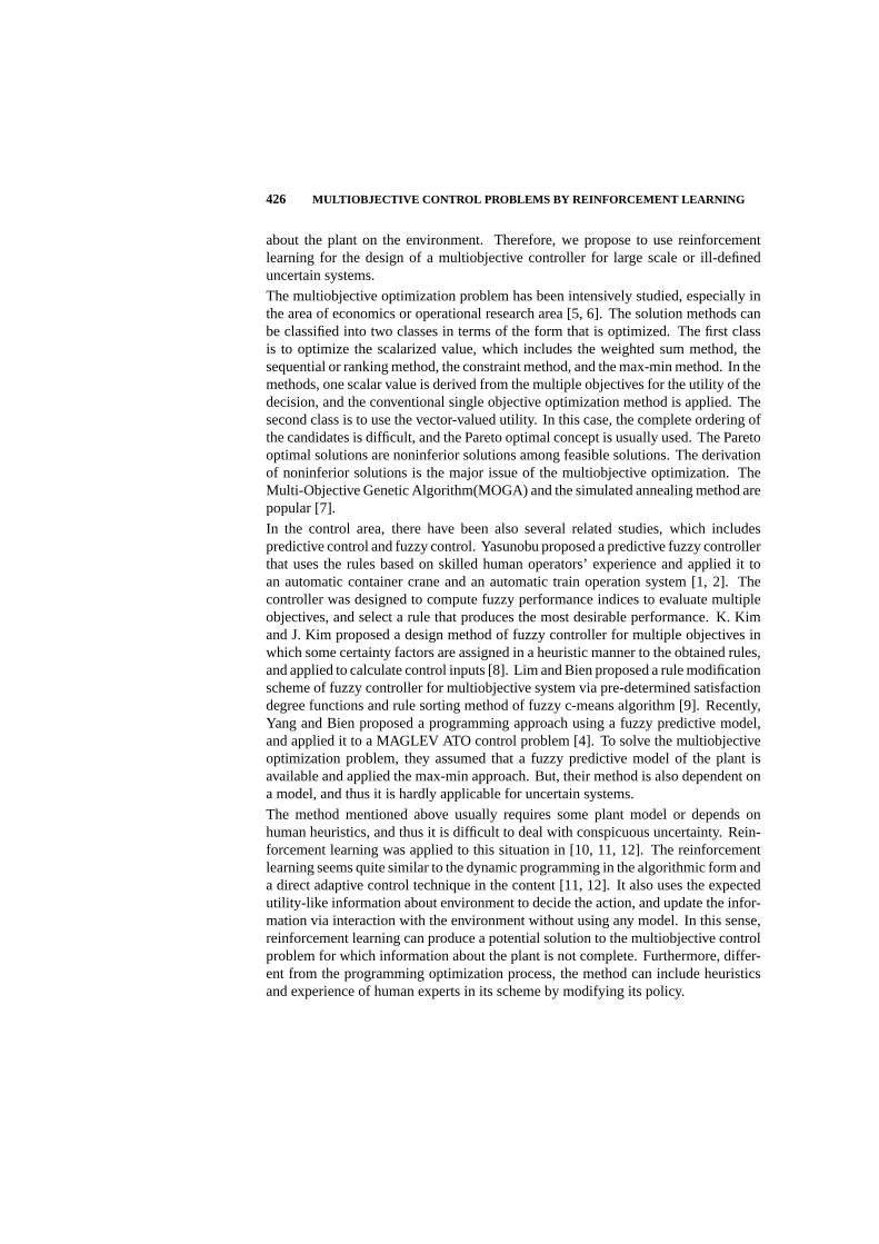
426 MULTIOBJECTIVE CONTROL PROBLEMS BY REINFORCEMENT LEARNING
about the plant on the environment. Therefore, we propose to use reinforcementlearning for the design of a multiobjective controller for large scale or ill-defineduncertain systems.
The multiobjective optimization problem has been intensively studied, especially inthe area of economics or operational research area [5, 6]. The solution methods canbe classified into two classes in terms of the form that is optimized. The first classis to optimize the scalarized value, which includes the weighted sum method, thesequential or ranking method, the constraint method, and the max-min method. In themethods, one scalar value is derived from the multiple objectives for the utility of thedecision, and the conventional single objective optimization method is applied. Thesecond class is to use the vector-valued utility. In this case, the complete ordering ofthe candidates is difficult, and the Pareto optimal concept is usually used. The Paretooptimal solutions are noninferior solutions among feasible solutions. The derivationof noninferior solutions is the major issue of the multiobjective optimization. TheMulti-Objective Genetic Algorithm(MOGA) and the simulated annealing method arepopular [7].
In the control area, there have been also several related studies, which includespredictive control and fuzzy control. Yasunobu proposed a predictive fuzzy controllerthat uses the rules based on skilled human operators’ experience and applied it toan automatic container crane and an automatic train operation system [1, 2]. Thecontroller was designed to compute fuzzy performance indices to evaluate multipleobjectives, and select a rule that produces the most desirable performance. K. Kimand J. Kim proposed a design method of fuzzy controller for multiple objectives inwhich some certainty factors are assigned in a heuristic manner to the obtained rules,and applied to calculate control inputs [8]. Lim and Bien proposed a rule modificationscheme of fuzzy controller for multiobjective system via pre-determined satisfactiondegree functions and rule sorting method of fuzzy c-means algorithm [9]. Recently,Yang and Bien proposed a programming approach using a fuzzy predictive model,and applied it to a MAGLEV ATO control problem [4]. To solve the multiobjectiveoptimization problem, they assumed that a fuzzy predictive model of the plant isavailable and applied the max-min approach. But, their method is also dependent ona model, and thus it is hardly applicable for uncertain systems.
The method mentioned above usually requires some plant model or depends onhuman heuristics, and thus it is difficult to deal with conspicuous uncertainty. Rein-forcement learning was applied to this situation in [10, 11, 12]. The reinforcementlearning seems quite similar to the dynamic programming in the algorithmic form anda direct adaptive control technique in the content [11, 12]. It also uses the expectedutility-like information about environment to decide the action, and update the infor-mation via interaction with the environment without using any model. In this sense,reinforcement learning can produce a potential solution to the multiobjective controlproblem for which information about the plant is not complete. Furthermore, differ-ent from the programming optimization process, the method can include heuristicsand experience of human experts in its scheme by modifying its policy.

PRELIMINARY 427
In this Chapter, the multiobjective control problem is studied in which the plant withuncertain dynamics will be dealt with by a fuzzy logic-based decision making system,and reinforcement learning is adopted for design of an on-line multiobjective fuzzylogic controller. In Section 17.2, we review several important preliminary subjectsincluding multiobjective optimization, and reinforcement learning. In Section 17.3,the policy improvement algorithm for Markov decision process with multiple rewardis scrutinized. In Section 17.4, we apply the algorithm proposed in Section 17.3 tomodel-free multiple reward reinforcement learning for fuzzy control. And, finally,some concluding remarks are given in the last section.
17.2 PRELIMINARY
17.2.1 Multiobjective Control and Optimization
Consider the MIMO plant with a controller which is dictated by multiple objectiveas shown in Figure 17.1.
Fig. 17.1 Multiobjective control problem.
A general multiobjective control problem may be stated as a functional minimizationproblem as follows:
min Q1(x(·),u(·)), Q2(x(·),u(·)), · · · , QM (x(·),u(·))s.t. gi(x(·),u(·)) ≤ 0, i = 1, · · · , I,
hj(x(·),u(·)) = 0, j = 1, · · · , J, (17.1)
wherex(·) is a state function of the plant, andu(·) is a control input.Qk are objectivefunctions,M is the number of objective functions,gi ≤ 0 are inequality constraints,

428 MULTIOBJECTIVE CONTROL PROBLEMS BY REINFORCEMENT LEARNING
I is the number of inequality constraints,hj = 0 are equality constraints, andJ isthe number of equality constraints. When the underlying variablesx(·) andu(·) arereal-valued, the problem is, in general, quite complicated to handle. In this paper, weassume that the system under consideration can be discretized for proper modellingso that the problem can be handled as a discrete valued problem.
A general discrete valued multiobjective optimization problem can be mathematicallydefined as follows:
min Q1(x), Q2(x), · · · , QM (x)s.t. x ∈ X ≡ x ∈ Rn|gi(x) ≤ 0, i = 1, · · · , I, hj(x) = 0, j = 1, · · · , J,
(17.2)
wherex ∈ Rn is a design variable,Qk(x) are objective functions,M is the numberof objective functions,gi(x) ≤ 0 are inequality constraints,I is the number ofinequality constraints,hj(x) = 0 are equality constraints, andJ is the number ofequality constraints.
If we directly apply the concept of the optimality used in the single-objective problemsto this multiobjective one, we arrive at the notion of a complete optimal solution [5, 6].
Definition 17.2.1 : Complete optimal solution [5]. A solutionx∗ is called acomplete optimal solution or ideal optimal solution to the problem in (17.2) , if , forall x ∈ X, there existsx ∈ X such thatQk(x∗) ≤ Qk(x), k = 1, 2, · · · ,M .
In general, such a complete optimal solution that simultaneously minimizes all themultiple objective functions may not exist, especially when some of objective func-tions conflict with the others. Thus, instead of a complete optimal solution, anothertype of optimal solution, called a Pareto optimal solution, is often sought.
Definition 17.2.2 : Pareto optimal solution [5]. A solutionx∗ is called a Paretooptimal solution or noninferior solution, if there does not existx ∈ X − x∗ suchthatQk(x) ≤ Qk(x∗), k = 1, 2, · · · ,M, andQk(x) < Qk(x∗) for at least onek.
The concept of the Pareto optimal solution is depicted in Figure 17.2.
There are a number of methods to get a Pareto optimal solution in multiobjective op-timization problems; the min-max method, the weighted sum method, the constraintmethod, and the goal programming are typical examples [5]. The methods derive onerepresentative objective from multiple objectives and optimize the objective usingsingle-objective optimization methods. The methods find the Pareto optimal solu-tions as depicted in Figure 17.3. Especially, the min-max method gives the singlesolution and is also applicable for non-convex problems [4, 5].
17.2.2 Makov Decision Process with Multiple Reward
In conventional reinforcement learning, the reward from the environment is a scalarvalue. In order to handle multiobjective problem, the scalar reward may not beeffective. The multiple rewards can be more suitable, corresponding to multiple
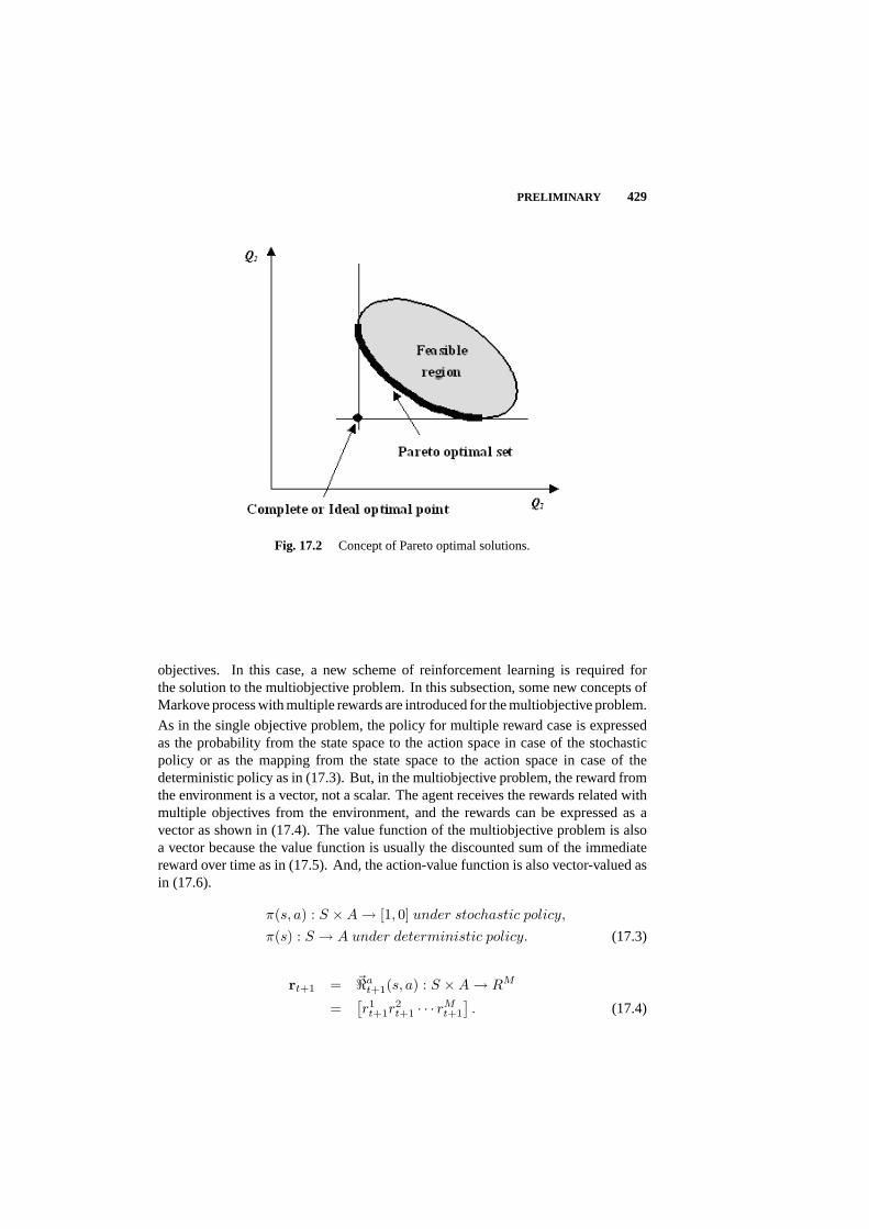
PRELIMINARY 429
Fig. 17.2 Concept of Pareto optimal solutions.
objectives. In this case, a new scheme of reinforcement learning is required forthe solution to the multiobjective problem. In this subsection, some new concepts ofMarkove process with multiple rewards are introduced for the multiobjective problem.
As in the single objective problem, the policy for multiple reward case is expressedas the probability from the state space to the action space in case of the stochasticpolicy or as the mapping from the state space to the action space in case of thedeterministic policy as in (17.3). But, in the multiobjective problem, the reward fromthe environment is a vector, not a scalar. The agent receives the rewards related withmultiple objectives from the environment, and the rewards can be expressed as avector as shown in (17.4). The value function of the multiobjective problem is alsoa vector because the value function is usually the discounted sum of the immediatereward over time as in (17.5). And, the action-value function is also vector-valued asin (17.6).
π(s, a) : S ×A → [1, 0] under stochastic policy,
π(s) : S → A under deterministic policy. (17.3)
rt+1 = ~<at+1(s, a) : S ×A → RM
=[r1t+1r
2t+1 · · · rM
t+1
]. (17.4)
430 MULTIOBJECTIVE CONTROL PROBLEMS BY REINFORCEMENT LEARNING
Fig. 17.3 Other examples of Pareto optimal solutions.
V(s) = E(∞∑
k=0
γkrt+k+1|st = s) where 0 ≤ γ < 1
= [V1 V2 · · ·VM ] . (17.5)
Q(s, a) = [Q1 Q2 · · · QM ]T . (17.6)
Here,S is the set of possible states,A the set of available actions,M the number ofobjectives, andγ is the discount rate.
In case of the multiobjective problem, it is difficult to order the elements of a set of thesolutions because of their multiple criteria. Instead, Pareto optimality often utilizedto embrace the difficulty caused by multiplicity of criterion [5, 6]. The concept ofPareto optimality is applicable for multiple reward reinforcement learning. To bespecific, the domination relation among the solutions is first defined as follows:
Definition 17.2.3 : Domination [5]. A vectorx ∈ RM is said to dominate a vectory ∈ RM if every element ofx is larger than or equal to the corresponding elementof y , and there exists at least one element ofx that is larger than the corresponding

PRELIMINARY 431
element ofy. Formally, we write
x >p y ⇔ (∀i, xi ≥ yi) and (∃i, xi > yi), i = 1, · · ·M, (17.7)
wherex = [x1x2 · · ·xM ]T , y = [y1y2 · · · yM ]T . Based on this concept, we candefine Pareto optimal set of vector-valued state-value functions as follows:
Definition 17.2.4 : Pareto optimal set of vector-valued state-value functions.
Optp [V] = V∗ ∈ VT| There exists no V ∈ VT,
s.t. V(s) >p V∗(s) for all s ∈ S, (17.8)
whereVT is the set of all possible value functions andx >p y meansx dominatesy . Together with Pareto optimal set of vector-valued state-value functions, we candefine Pareto optimal set of the vector-valued action-value functions as follows:
Definition 17.2.5 : Pareto optimal set of vector-valued action-value functions.
Optp [Q] = Q∗ ∈ QT| There exists no Q ∈ QT,
s.t. maxa
Q(s, a) >p maxa
Q∗(s, a), for all s ∈ S, (17.9)
whereQT is the set of all possible vector-valued action-value functions.
Definition 17.2.6 : Pareto optimal policy. A policyπp is called Pareto optimal ifand only if the resulting vector-valued state-value function is a member of the Paretooptimal set of vector-valued state-value functions. LetΠp denote Pareto optimalpolicies, that is,
Πp = πp ∈ Π| There exists no π ∈ Π ,
s.t. Vπ(s) >p Vπp
(s), for all s ∈ S, (17.10)
whereVπ is a vector-valued state-value function when a policyπ is adopted, andΠ is a set of possible policies. It is remarked that the Pareto optimal set of thevector-valued state-value functions or the vector-valued action-value functions maycontain more than one element. Different from the single reward case, thus, therecan be multiple Pareto optimal candidates.
From the perspective of Pareto optimality, we can define the concept of multiplereward reinforcement learning, which, given the rewards from the environment, isconcerned with derivation of the Pareto optimal policy and value function. From themultiobjective optimization technique explained in the previous Subsection, we cansay that if the max-min approach is applied to derive a policy of the multiple rewardreinforcement learning problem, we may get the Pareto optimal policy. In fact, themethod of the max-min multiobjective optimization technique is used for the solutionof the multiple reward reinforcement learning in the present Chapter.
We remark that the ordinary reinforcement learning can treat the multiobjectiveproblem by letting the goal of the learning as the coset of the solution of each
432 MULTIOBJECTIVE CONTROL PROBLEMS BY REINFORCEMENT LEARNING
objective [13]. But, different from the ordinary reinforcement learning, the multiplereward reinforcement learning enables us to get the Pareto optimal policy morelogically because it takes into account the trade-off information among the multipleobjectives. Furthermore, the multiple reward reinforcement learning is expected toresult in the fast convergence of the learning process by considering the multipleobjectives.
17.3 POLICY IMPROVEMENT ALGORITHM FOR MDP WITHVECTOR-VALUED REWARD
17.3.1 Multiobjective Dynamic Programming
In this Subsection, the method of multiobjective dynamic programming is proposedas a tool for the multiobjective optimization. The proposed multiobjective dynamicprogramming guarantees Pareto optimality of solution. To proceed, we first define aconcept called value difference, which is concerned with the scalar value function.Later, we shall consider the vector value case.
The value difference is the difference between the action-value of each possible actionand the state-value of the current policy. LetQπt(x, πt+1(x)) be the action-valuefunction when the actionπt+1(x) is taken via the current policyπt at the statex ,V πt the state-value function of the current policyπt at the statex, and4(x, πt+1(x))the difference between them. Then, we call the quantity4(x, πt+1(x)) the valuedifference.
Definition 17.3.1 : Value difference.
4(x, πt+1(x)) = Qπt(x, πt+1(x))− V πt(x)
=
Qπt((x), πt(x))− V πt(x) = 0, if x 6= s,Qπt(s, πt+1(s))− V πt(s) ≡ 4(s, πt+1(s)), if x = s,
(17.11)
whereQπt(s, πt+1(x)) = EπtRt =∑∞
k=0 γkrt+k+1|st = x, at = πt+1(x).Regarding the single value function, we choose the action as the new policy for thestate, whose value difference is positive. The method increases the state value ofthe updated policy. Note that, if we choose the action whose the value difference isnegative, the state value of the new policy decreases. In case the value difference iszero, the state value does not change. From this perspective, the following Lemma17.3.1 is derived.
Lemma 17.3.1 Upper/Lower Bound forV πt+1(s).
If 4(s, a) > 0 andπt+1(s) = a , thenV πt(s) + 4(s,a)1−γ > V πt+1(s) > V πt(s) +
4(s, a) > V πt(s) , and if4(s, a) < 0 , thenV πt(s) + 4(s,a)1−γ < V πt+1(s) <
V πt(s) +4(s, a) < V πt(s). If 4(s, a) = 0, thenV πt+1(s) = V πt(s).
POLICY IMPROVEMENT ALGO. FOR MDP WITH VEC-VALUED REWARD 433
Proof) The proof can be referred in the Appendix. ¥As a result, if the value difference is kept positive by updating the policy, the overallstate value of the policy increases. This means that we will get an optimal policy asLemma 17.3.1 shows. From Lemma 17.3.1, we get the bound of the change of thestate-value function by policy update.
In Lemma 17.3.1, the bound of the scalar state-value function is derived. In caseof multiple objectives, the bound of the state-value function of each objective isderived from Lemma 17.3.1. By using these multiple bounds of multiple state-valuefunctions, the dynamic programming algorithm is extended to the case of multipleobjectives. Based on the value differences of the multiple objectives, the proposedmultiobjective dynamic programming algorithm is derived as follows:
πt+1(x) =
πt(x), x 6= s,a∗, x = s,
(17.12)
where
a∗ =
arg max1≤i≤M [4i(s, a)] ,if 4k(s, a) = 0 and4j(s, a) ≥ 0,
where k = arg min1≤i≤M
[V
πt(s)i
]for all a ∈ A(s), all j 6= k, 1 ≤ j ≤ M,
arg maxa min1≤i≤M
[V
πt(s)i +4i(s, a)
]= arg maxa min1≤i≤M [Qπt
i (s, a)] ,elsewhere,
Here,s is the current state,M is the number of objectives, and4i(s, a) is the valuedifference of theith objective at the states and actiona.
The proposed method changes the policy incrementally. That is, the policy is updatedby changing the action for the current state, and after the state transition, the actionfor the next transited state is updated. Therefore, the actions which are dedicated forthe other states in the updated policy are the same as the actions in the current policy.This property enables us to update the policy on-line.
The proposed method is based on the max-min optimization technique, which updatesthe policy and gives the bigger minimum objective than the one which the originalpolicy gives.
Lemma 17.3.2 The policy updated via max-min optimization has the bigger mini-mum objective than the one which the original policy gives, that is,
maxa
min1≤i≤M
[V πti (s) +4i(s, a)] ≥ min
1≤j≤MV πt
j (s).
Proof) The proof can be referred in the Appendix. ¥
434 MULTIOBJECTIVE CONTROL PROBLEMS BY REINFORCEMENT LEARNING
Based on Lemma 17.3.1 and Lemma 17.3.2, we can prove an important theoremin the dynamic programming method which is the policy improvement theorem.In the single objective case, the theorem guarantees the improvement of the statevalue of the policy updated by the dynamic programming. Similarly, in case of themultiple objectives, the minimum value among the multiple objectives is guaranteedto be nondecreasing. This guarantees that the proposed multiobjective dynamicprogramming method gives a nondecreasing minimum value among the multipleobjectives.
Theorem 17.3.1 : Multiobjective Policy Improvement Theorem.
min1≤i≤M
V πti (s) ≤ min
1≤i≤MV
πt+1i (s)
if s is not visited again after timet. Here,M is the number of multiple objectives.
Proof) The proof can be referred in the Appendix. ¥The theorem guarantees the nondecreasing property of the minimum value amongmultiple objectives. Figure 17.4 shows the resultant value function trends due to theproposed multiobjective dynamic programming. The state value of the present stateis nondecreasing after update by the proposed method.
In the theorem, we assume that the present states should not be visited again afterthe present timet. In the realistic control problem, the state at the present timetis not revisited unless the state is a stable equilibrium state or the state in the limitcycle. Therefore, the assumption which is used in Theorem 1 is not too restrictive.In case of the stochastic environment, however, every state may be visited after thepolicy update is performed.
The following theorem shows the relation between the value difference and thePareto optimal solution. If the value difference is zero for all states and objectives,the solution is Pareto optimal. This means that if the value difference is zero for allstates and objectives, there is no improvement by the policy update. Therefore, thesolution is optimal.
Theorem 17.3.2 If 4i(s, πt+1(s)) = 0 for any1 ≤ i ≤ M , s, thenπt+1 is a Paretooptimal solution.
Proof) The proof can be referred in the Appendix. ¥The following three corollaries show that the proposed method diminishes the valuedifferences of the objectives, and finally gives a sub Pareto optimal solution.
Corollary 17.3.1 The upper bound of4ti(s, a) for a states is nonincreasing as time
t increases, where4ti(s, a) is the value difference of the objectivei at the timet.
Proof) The proof can be referred in the Appendix. ¥
Corollary 17.3.2 The lower bound of4ti(s, a) for a state s is nondecreasing as time
t increases.
Proof) The proof can be referred in the Appendix. ¥

MODEL-FREE MULTIPLE REWARD RL FOR FUZZY CONTROL 435
Fig. 17.4 State-value trend by the proposed mutiobjective dynamic programming.
Corollary 17.3.3 The bound of the difference between
max1≤i≤M
V πti (s) and min
1≤j≤MV πt
j (s) is nonincreasing for a state s as time t increases.
Proof) The proof can be referred in the Appendix. ¥Because the upper bounds of the value differences diminish, the value differenceswill be nonincreasing, and remain within a certain value. This means the policyupdated by the proposed method will be similar to the Pareto optimal solution withina certain bound.
17.4 MODEL-FREE MULTIPLE REWARD REINFORCEMENTLEARNING FOR FUZZY CONTROL
In the previous Subsection, we have assumed that the model of the environment exists.If the model is not available, or inaccurate, the multiobjective dynamic programmingmay not be directly applicable for the mutiobjective control problem. In this Section,a model-free reinforcement learning scheme is proposed. When the model is absent,the state value function is obtained using the temporal difference learning. In thisSection, the model-free multiple reward reinforcement learning schemes are appliedfor designing a fuzzy controller of a multiobjective control problem.
436 MULTIOBJECTIVE CONTROL PROBLEMS BY REINFORCEMENT LEARNING
17.4.1 Multiple Reward Adaptive Critic Reinforcement Learning
The adaptive heuristic critic is popular in reinforcement learning [11, 12]. Theadaptive critic is used to estimate the state value function. The adaptive critic and thepolicy are updated via the temporal difference learning. The same adaptive heuristiccritic scheme is similarly applicable to the multiple reward reinforcement learningproblem. In this Chapter, the multiple adaptive critics are adopted for the estimationof the state-value functions for the multiple rewards. And, the policy is updatedvia the temporal difference which is selected among the temporal differences forthe multiple rewards. The overall structure of the multiple reward adaptive criticreinforcement learning is depicted in Figure 17.5. For each reward, the state valuefor the reward is estimated. For every action, the temporal differences of the multiplerewards are obtained as follows:
δj = rjt + γVj(st)− Vj(st−1), j = 1, · · · ,M, (17.14)
wherest is the state at the timet, rjt is the reward for thejth objective,δj is the
temporal difference for thejth reward,Vj(s) is the estimated state value function ofthe states for the jth reward, andM is the number of the objective. So, for eachadaptive critic, the state value function is updated using each temporal difference asfollows:
Vj(s) = Vj(s) + αδj , if s = st−1,
Vj(s) = Vj(s), otherwise,(17.15)
whereα is the learning rate, andj = 1, · · · ,M . For the policy, one of the temporaldifferences for the rewards is selected. In this Chapter, based on the multiobjectivedynamic programming proposed in the previous Subsection, the temporal differencefor the update of the policy is selected as follows:
δp = δk, (17.16)
where
k =
arg max δi,
if δm = 0 for m = arg miniV i(st)), or ∀j, δj ≥ 0 and ∃`, δ` > 0,
arg miniV i + δi, otherwise.
The policy has the quality parameters for each action. The selected temporal differ-ence is used to update the quality parameter as follows:
Q(s, a) = Q(s, a) + βδp, (17.18)
whereQ(s, a) is the quality of the action a for the states, andβ is the learning rate.In the policy, the quality parameters are used to modulate the probability of the actionselection. There are various probability distribution of the selection of the action forthe policy in the reinforcement learning area [14]. The probabilistic policy is adopted

MODEL-FREE MULTIPLE REWARD RL FOR FUZZY CONTROL 437
for both exploration and exploitation. In the Chapter, theε-greedy selection methodis adopted [14].
Fig. 17.5 Overall Structure of the multiple reward adaptive critic reinforcement learning .
17.4.2 Adaptive Fuzzy Inference System
As discussed in the previous Section, the multiple reward reinforcement learningscheme is constructed on the bases of the discrete states and actions. And, the state-value function and the action-value function are used for the optimization. And,the policy is a rule which correlates the states with actions. In the multiple rewardreinforcement learning for the multiobjective control problem, we need a functionapproximation structure for the state-value function, and controller for the policyfor the continuous state and action. That is, because the continuous state spacerequires the continuous output of the state value function, the function approximationis used for the state-value function prediction. The neural networks and neuro-fuzzy systems are popular methods for the purpose. Especially, the neuro-fuzzysystem is suitable for using the expert knowledge. In this Section, we adopt a
438 MULTIOBJECTIVE CONTROL PROBLEMS BY REINFORCEMENT LEARNING
fuzzy inference system to implement the critics and the policy of the multiobjectiveadaptive critic. The fuzzy inference system enables us to utilize the knowledge whichis possibly obtained from human experts. And, since the learning mechanism needsan adaptive structure, we use an adaptive fuzzy inference system proposed by Jouffe[14]. Jouffe proposed the multiple consequent term fuzzy controller and the fuzzyinference system with singleton consequent fuzzy sets for value function prediction.He applied the reinforcement learning for updating the controller [14]. The Jouffe’sfuzzy inference system has multiple consequent terms for each fuzzy rule, whichis equivalent to the rule base with inconsistent rules. As shown by Yu and Bien,the fuzzy logic controller with inconsistent rule-base can have a better performance[15]. As such, we use the Jouffe’s adaptive fuzzy inference system structure for themultiobjective fuzzy logic controller.
The fuzzy inference system is composed of four layers as depicted in Figure 17.6 .Each layer of the fuzzy inference system has the following function:
Layer 1) Input layer.
Layer 2) Membership calculation of each antecedent term.
Layer 3) Rule base node. It connects the input from the layer 2 to the output.
Layer 4) In the node, the defuzzification is performed and the final output of the fuzzycontroller is determined.
In this paper, the singleton output fuzzy terms are used, and the center-averagedefuzzification is adopted as:
y =∑N
i=1 yiµi(x)∑Ni=1 µi(x)
, (17.19)
whereN is the number of rules,yi is the consequent singleton term of the rulei,µi(x) is the firing strength of the rulei andx is the input variable.
Each output of the adaptive critics is the predicted state-value function as:
Vj,t(S(t)) = vj,tΦTt =
∑Ni=1 vi,jµi(S(t))∑N
i=1 µi(S(t)), (17.20)
wherej = 1, · · · ,M is the index for the objective,M is the number of objective,vj,t = [v1,jv2,j · · · vN,j ] is the vector of the output singleton terms for each critic,
Φt =[
µ1(S(t))∑Ni=1 µi(S(t))
µ2(S(t))∑Ni=1 µi(S(t))
· · · µN (S(t))∑Ni=1 µi(S(t))
]is the vector of the truth values
of each rule,S(t) is the state of the environment at timet. In the systems, themultiple adaptive critics share the common antecedent part with each other and thepolicy fuzzy controller as depicted in Figure 17.8.
In the fuzzy controller which implements a policy, each rule has multiple consequentterms for each rule as follows:

MODEL-FREE MULTIPLE REWARD RL FOR FUZZY CONTROL 439
Ri : If s1 is Li1 and · · · and sN is Li
N , then u is U i,1, U i,2, · · · , U i,p,(17.21)
whereS = s1, · · · , sN is a set of input variables,N is the number of inputvariables,Li
1, · · · , LiN is a fuzzy set of antecedent of rulei, andu is the output
variable, whileU i,1, U i,2, · · · , U i,p is a term set of consequent of rulei, p is thenumber of terms in the consequent. It is noted that, the output consequent in (17.21)is not just a single constant term as in usual Takagi-Sugeno-Kang representation but ap-tuple of numbers. At any instance, the only one output consequent term should beselected in the scheme. The concept of the multiple consequent terms is depicted inFigure 17.7. The utilityQi,k is assigned to each output consequent termU i,k . And,for each rule, one output consequent term among ap-tuple of consequent terms isselected in consideration of the expected utilitiesQi,k of actionsU i,k, k = 1, · · · , p.The method to select one output consequent term for each rule is described in detailin [14]. After selecting one consequent termU i for each rule, the scheme calculatesthe final controller output as follows:
u =∑N
i=1 U iµi(S)∑Ni=1 µi(S)
. (17.22)
The utilities Qi,k are the parameters of the actor, that is, the parameters of theassociative search element in an adaptive heuristic critic structure. They are updatedat every action. Therefore, in the adaptive fuzzy inference system, the parameters toadjust are the consequent singletons of the multiple adaptive critics and the policyfuzzy controller :vj,t, Q
i,kt .
17.4.3 Multiple Reward Adaptive Critic Reinforcement Learning for FuzzyControl
We apply the proposed multiple reward adaptive critic reinforcement learning to theadaptive fuzzy inference system introduced earlier. The overall learning algorithm isdescribed as follows:
Step 1) Calculate the state value function of each critic using the current evaluationfunction fuzzy system as follows:
Vj,t−1(St) = vj,t−1ΦT (St), (17.23)
wherej = 1, · · · ,M is the index for the objective,M is the number of objectives,andSt is the state at timet.
Step 2) Compute the temporal differences of the critics. And, as the feedback valueto the fuzzy controller, select one which has the minimum state-value among themas follows:

440 MULTIOBJECTIVE CONTROL PROBLEMS BY REINFORCEMENT LEARNING
Fig. 17.6 Adaptive Fuzzy Inference System whereNi: number of the input variables,N :number of the rules,No: number of the outputs [14].
Fig. 17.7 Multiple output term case for each rule.
δjt = rj
t + γVj,t−1(St)− Vj,t−1(St−1), j = 1, · · · ,M,
δpt = δk
t ,

MODEL-FREE MULTIPLE REWARD RL FOR FUZZY CONTROL 441
Fig. 17.8 Fuzzy controller using AFIS [14].
where
k =
arg max δit,
if δmt = 0 for m = arg miniV i
t−1) and∀j, δjt ≥ 0 and ∃`, δ`
t > 0,
arg miniV it−1 + δi
t,otherwise.
(17.24)
Here,γ is the discount rate, andrjt is the reward of thejth objective at timet.
Step 3) Update the parameter vectors of the fuzzy inference systems as follows:
vjt = vj,t−1 + βδjt φt−1, j = 1, · · · , M,
QUi,k
t = QUi,k
t−1 + ϕδpt e
Ui,k
t−1 , i = 1, · · · , N, k = 1, · · · , q, (17.25)
whereβ andϕ are learning rates,eUi,k
t andφt =[φ1 φ2 · · · φN
]are the eligibility
traces of the utility of the action and the value function [14].
Step 4) Calculate the values of the state using the updated evaluation function net-works as follows:
Vj,t(St) = vj,tΦT (St), (17.26)
whereVj,t means the output of each critic after the parameters are updated.

442 MULTIOBJECTIVE CONTROL PROBLEMS BY REINFORCEMENT LEARNING
Step 5) Update the eligibility traces as follows:
Φt = Φt + γλΦt−1,
ei,kt (U i) =
λ′ei,k
t−1 + φRi(St), if U i
t = U i,k,
λ′ei,kt−1, otherwise,
(17.27)
where λ is the eligibility rate, λ′ is the actor recency factor, andφRi(St) =µi(St)∑N
j=1 µj(St)is the truth value of rule i, andU i
t is the selected fuzzy consequent
singleton of fuzzy rulei, i = 1, · · · , N .
Step 6) Select the new actionUt and take the action as follows:
Ut =∑N
i=1 U itµi(St)∑N
i=1 µi(St), (17.28)
where the selection process is the stochastic selection, that is,ε-greedy selection,which is explained in Jouffe [14].
Fig. 17.9 Structure of multiple reward reinforcement learning .
17.4.4 Simulation
To show the effectiveness of the proposed method, some simulation is conducted forthe inverted cart pole as depicted in Figure 17.10. It is the fourth order system, andthe goals of the system are

MODEL-FREE MULTIPLE REWARD RL FOR FUZZY CONTROL 443
1) Erect the pole upright and keep it upright.
2) The position of the cart should not be far away from the reference position.
As one can see, the two objectives can be conflicting in many situations. Thus, it is agood example of the multiobjective problem. The state equation of the system is asfollows:
x(t + 1) = x(t) + Tf(x(t)) + g(x(t))u(t),f(x) = [f1(x) f2(x) f3(x) f4(x)]T ,
f1(x) = θ,
f2(x) =g sin θ − cos θ
[m`θ2 sin θ − µcsgn(x)
]/(mc + m)− µpθ/m`
` [3/4−m cos2 θ/(mc + m)],
f3(x) = x,
f4(x) =m`
[θ2 sin θ − θ cos θ
]− µcsgn(x)
mc + m,
g(x) = [g1(x) g2(x) g3(x) g4(x)]T ,
g1(x) = 0, g2(x) =− cos θ
` [3/4−m cos2 θ/(mc + m)],
g3(x) = 0, g4(x) =1
mc + m,
x =[θ θ x x
], (17.29)
wherex is the position of the cart,x is the velocity of the cart,θ is the angle of thepole, andθ is the angular velocity of the pole.
Fig. 17.10 The inverted cart pole system.

444 MULTIOBJECTIVE CONTROL PROBLEMS BY REINFORCEMENT LEARNING
The parameters of the inverted cart are as follows:
mc = 1Kg : mass of the cart.m = 0.1Kg : mass of the pole.` = 0.5m : length of the pole.Ts = 0.02sec : sampling time.µc = 0.0005 : friction coefficient of cart on the track.µp = 0.0005 : friction coefficient of pole on the cart.g = 9.8m/sec2 : constant of gravity.
(17.30)
The objectives of the system are that the system is kept in the area of|θ| ≤ 12 and|x| ≤ 1m . And, the following rewards are given as:
If |θ| ≥ 12, thenr1 = 0, elser1 = −1 . If |θ| ≥ 1m, thenr2 = 0, elser2 = −1.
The task of the inverted pendulum is an episodic task, and if the failure occurs, thestate is reset to the initial state.
The parameters of the learning algorithm for the system areγ = 0.95, λ = 0.9,λ′ = 0.9, β = 0.01, ϑ = 0.01 . We use3× 3× 3× 3 = 81 rules for input variables.The output of the controller is restricted in|u| ≤ 10N .
Fig. 17.11 Comparison with single objective case (average failures).
Figure 17.11 compares several methods using the time step for success when theinitial posture of the inverted pendulum is (0,0,0,0). The average failures over 100

SUMMARY 445
Fig. 17.12 Comparison with single objective case (computation time) .
runs are shown in Figure 17.11. As one can see, the proposed method is superioras the number of the consequent singleton increases. Barto’s method uses twooutput choices such as bang-bang control, and shows somewhat poor results of76.2 average failures [11]. Figure 17.12 shows the computation time for severalmethods. The Pentium II 450MHz processor is used to calculate the computationtime of the methods. Barto uses the box system for the input space partition, andthe box system requires little computation. In case of a fuzzy inference system, thecalculation of the fuzzy firing strength requires some computation time. Therefore,the proposed method takes more time than the Barto’s method. And, the proposedmethod uses the multiobjective prediction, and therefore, the computation for themultiple objective is required. That means the computation for the proposed methodrequires more time than the single objective case. However, Figure 17.12 shows thatthis method incurs only the very modest worst-case computational penalty of 33%over the single objective case. As the number of consequent singleton increases, therelative computational penalty gets small, i.e., 5% in case of 9 consequent singletons.
17.5 SUMMARY
In this Chapter, we have proposed a reinforcement learning technique to be appliedfor multiobjective control problem. The multiobjective dynamic programming isconsidered for multiobjecitve optimization of the policy, and its max-min optimiza-tion is applied for multiple reward reinforcement learning in selecting the feedbacktemporal difference among multiple temporal differences of rewards. Using the adap-tive fuzzy inference structure, the multiple reward reinforcement learning is extended

446 MULTIOBJECTIVE CONTROL PROBLEMS BY REINFORCEMENT LEARNING
to the fuzzy controller for a multiobjective control problem. Some simulation resultsare given to show the effectiveness of the proposed method.
We remark that the issues on the convergence of the proposed method to the Paretooptimality and the relation between the parameters of reinforcement learning and thecontrol results remain to be further studied.

Bibliography
1. S. Yasunobu and T. Hasegawa, “Evaluation of an automatic container crane op-eration system based on predictive fuzzy control,”Control Theory and AdvancedTechnology,Vol. 2, pp. 419-432, 1986.
2. S. Yasunobu and S. Miyamoto, “Automatic train operation system by predictivefuzzy control,” in Industrial Application of fuzzy control (M.Sugeno eds.), pp.1-18, North-Holland: Elsevier Science Publishers, 1985.
3. Y. S. Song, “Design of Fuzzy Sensor-based Fuzzy Combustion Control Systemfor Refuse Incinerator,” Master Thesis paper in KAIST, Dept. of Automation andDesign Engineering, 1997.
4. Z. Bien, D. Kang, and S. Yang, “Progrmming Approach for fuzzy model-basedMultiobjective Control Systems,”International Journal on Fuzziness, Uncer-tainty, and Knowledge-Based Reasoning,Vol. 7, No. 4, pp. 289-292, 1999.
5. Y. J. Lai and C. L. Hwang, “Fuzzy Multiple Objective Decision Making,”Springer-Verlag, Berlin, 1994.
6. M. Sakawa, “Fuzzy Sets and Interactive Multiobjective Optimization,” PlenumPress, New York, 1993.
7. C. M. Fonseca and P. J. Fleming, “Multiobjective genetic algorithms,”IEEColloquium on Genetic Algorithms for Control Systems Engineering,pp. 6/1-6/5, 1993.
8. K. Kim and J. Kim, “Multicriteria fuzzy control,”Journal of Intelligent andFuzzy Systems,Vol. 2, pp. 279-288, 1994.
9. T. Lim and Z. Bien, “FLC Design for Multi-Objective System,”Journal ofApplied Mathematics and Computer Science,vol. 6, no. 3, pp. 565-580, 1996.
10. R. S. Sutton, A. G. Barto, and R. J. Williams, “Reinforcement Learning is DirectAdaptive Optimal control,”IEEE Control Systems,pp. 19-22, 1992.
11. G. Barto, R. S. Sutton, and C. W. Andersonn, “Neuronlike Adaptive ElementsThat Can Solve Difficult Learning Control Problems,”IEEE Transactions onSystems, Man, and Cybernetics,Vol. SMC-13, No. 5, pp. 834-846, 1983.
447

448 BIBLIOGRAPHY
12. L. P. Kaebling, M. L. Littman, and A. W. Moore, “Reinforcement Learning: ASurvey,“Journal of Artificial Intelligence Research,Vol. 4, pp. 237-285, 1996.
13. Chin-Teng Lin and I-Fang Chung, “A reinforcement neuro-fuzzy combiner formultiobjective control,”IEEE Transactions on Systems, Man and Cybernetics,Part B, Vol. 29, No. 6, pp. 726-744, 1999.
14. L. Jouffe, “Fuzzy Inference System Learning by Reinforcement Methods,”IEEETransaction on Systems, Man, and Cybernetics,Part C, Vol. 28, No. 3, pp. 338-355, 1998.
15. Z. Bien and W. Yu, “Extracting core information from inconsistent fuzzy controlrules,”Fuzzy Sets and System,vol. 71, no. 1, pp. 95-111, April. 1995.
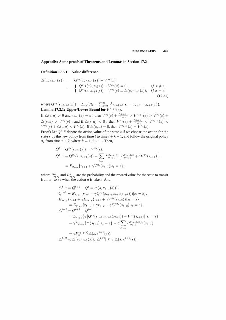
BIBLIOGRAPHY 449
Appendix: Some proofs of Theorems and Lemmas in Section 17.2
Definition 17.5.1 : Value difference.
4(x, πt+1(x)) = Qπt(x, πt+1(x))− V πt(x)
=
Qπt((x), πt(x))− V πt(x) = 0, if x 6= s,Qπt(s, πt+1(s))− V πt(s) ≡ 4(s, πt+1(s)), if x = s,
(17.31)
whereQπt(s, πt+1(x)) = EπtRt =
∑∞k=0 γkrt+k+1|st = x, at = πt+1(x).
Lemma 17.3.1: Upper/Lower Bound forV πt+1(s).
If 4(s, a) > 0 andπt+1(s) = a , thenV πt(s) + 4(s,a)1−γ > V πt+1(s) > V πt(s) +
4(s, a) > V πt(s) , and if4(s, a) < 0 , thenV πt(s) + 4(s,a)1−γ < V πt+1(s) <
V πt(s) +4(s, a) < V πt(s). If 4(s, a) = 0, thenV πt+1(s) = V πt(s).Proof) LetQt+k denote the action value of the states if we choose the action for thestates by the new policy from timet to timet+ k− 1, and follow the original policyπt from timet + k, wherek = 1, 2, · · · . Then,
Qt = Qπt(s, πt(s)) = V πt(s).
Qt+1 = Qπt(s, πt+1(s)) =∑st+1
Pπt+1(s)sst+1
[Rπt+1(s)
sst+1+ γV πt(st+1)
],
= Eπt+1rt+1 + γV πt(st+1)|st = s,
whereP as1s2
andRas1s2
are the probability and the reward value for the state to transitfrom s1 to s2 when the actiona is taken. And,
4t+1 = Qt+1 −Qt = 4(s, πt+1(s)).Qt+2 = Eπt+1rt+1 + γQπt(st+1, πt+1(st+1)))|st = s.Eπt+1rt+1 + γEπt+1rt+2 + γV πt(st+2)|st = s
= Eπt+1rt+1 + γrt+2 + γ2V πt(st+2)|st = s.4t+2 = Qt+2 −Qt+1
= Eπt+1γ [Qπt(st+1, πt+1(st+1))− V πt(st+1)] |st = s= γEπt+14(st+1)|st = s = γ
∑st+1
Pπt+1(s)sst+1
4(st+1)
= γPπt+1(s)ss 4(s, πt+1(s)).
4t+2 ∝ 4(s, πt+1(s)), |4t+2| ≤ γ|4(s, πt+1(s))|.
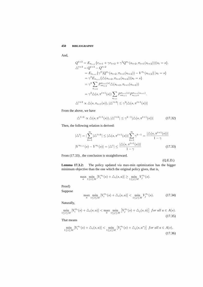
450 BIBLIOGRAPHY
And,
Qt+3 = Eπt+1rt+1 + γrt+2 + γ2Qπt(st+2, πt+1(st+2)))|st = s.4t+3 = Qt+3 −Qt+2
= Eπt+1γ2 [Qπt(st+2, πt+1(st+2))− V πt(st+2)] |st = s= γ2Eπt+14(st+2, πt+1(st+2))|st = s= γ2
∑st+2
Pπt+1(s)sst+2
4(st+2, πt+1(st+2))
= γ24(s, πt+1(s))∑st+1
Pπt+1(s)sst+1
Pπt+1(st+1)st+1s .
4t+3 ∝ 4(s, πt+1(s)), |4t+3| ≤ γ2|4(s, πt+1(s))|
From the above, we have
4t+k ∝ 4(s, πt+1(s)), |4t+k| ≤ γk−1|4(s, πt+1(s))| (17.32)
Then, the following relation is derived:
|4t| = |∞∑
k=1
|4t+k| ≤ |4(s, πt+1(s))|∞∑
k=1
γk−1 =|4(s, πt+1(s))|
1− γ
|V πt+1(s)− V πt(s)| = |4t| ≤ |4(s, πt+1(s))|1− γ
(17.33)
From (17.33) , the conclusion is straightforward.
(Q.E.D.)
Lemma 17.3.2: The policy updated via max-min optimization has the biggerminimum objective than the one which the original policy gives, that is,
maxa
min1≤i≤M
[V πti (s) +4i(s, a)] ≥ min
1≤j≤MV πt
j (s).
Proof)
Supposemax
amin
1≤i≤M[V πt
i (s) +4i(s, a)] < min1≤j≤M
V πtj (s). (17.34)
Naturally,
min1≤i≤M
[V πti (s) +4i(s, a)] < max
amin
1≤j≤M
[V πt
j (s) +4j(s, a)]
for all a ∈ A(s).
(17.35)That means
min1≤i≤M
[V πti (s) +4i(s, a)] < min
1≤j≤M
[V πt
j (s) +4j(s, a∗)]
for all a ∈ A(s),
(17.36)

BIBLIOGRAPHY 451
wherea∗ = arg max
amin
1≤j≤M
[V πt
j (s) +4j(s, a)].
From (17.34), (17.36), we can derive
min1≤i≤M
[V πti (s) +4i(s, a)] < min
1≤j≤M
[V πt
j (s) +4j(s, a∗)]
< min1≤k≤M
V πt
k (s) for all a ∈ A(s). (17.38)
If we choosea = a = πt(s) , then
4i(s, a) = 4i(s, πt(s)) = 0 for all i,
min1≤i≤M
[V πti (s) +4i(s, a)] = min
1≤i≤MV πt
i (s). (17.39)
From (17.38), (17.39),
min1≤i≤M
V πti (s) < min
1≤k≤MV πt
k (s). (17.40)
This is the contradiction. Therefore, we can conclude that
maxa
min1≤i≤M
[V πti (s) +4i(s, a)] ≥ min
1≤j≤MV πt
j (s).
¥Theorem 17.3.1: Multiobjective Policy Improvement Theorem.
min1≤i≤M
V πti (s) ≤ min
1≤i≤MV
πt+1i (s)
if s is not visited again after timet. Here,M is the number of multiple objectives.
Proof)
Case 1)
If 4k(s, a) = 0 and4j(s, a) ≥ 0 for all j and∃`,4`(s, a) 6= 0, where
k = arg min1≤i≤M
[V
π∗(s)i
]for all a ∈ A(s).
By Lemma 1, V πt
k (s) ≤ V πtj (s) ≤ V
πt+1j (s) and V πt
k (s) = Vπt+1k (s), then
Vπt+1k (s) ≤ V
πt+1j (s) .
Therefore,
min1≤k≤M
V πt
k (s) ≤ min1≤k≤M
Vπt+1k (s). (17.43)
Case 2)

452 BIBLIOGRAPHY
Let a∗ such that
a∗ = arg maxa
min1≤i≤M
[V
π∗(s)i +4i(s, a)
].
Then, by Lemma 2,
min1≤i≤M
Vπ∗(s)i ≤ min
1≤i≤M
[V
π∗(s)i +4i(s, a)
].
Therefore, if4m(s, a∗) ≥ 0 by Lemma 1,
V πtm (s)+
4m(s, a∗)1− γ
≥ V πt+1m (s) ≥ V πt
m (s)+4m(s, a∗) ≥ V πtm (s) ≥ min
iV πt
i (s).
(17.44)If 4m(s, a∗) < 0 , thenV
πt+1m (s) < V πt
m (s) by Lemma 1.
By assumption,V πt+1m (s) = V πt
m (s) +4m(s, a∗) for all s, m.
Therefore,
V πtm (s) +
4m(s, a∗)1− γ
< V πt+1m (s) = V πt
m (s) +4m(s, a∗) < V πtm (s) for all s.
(17.45)By Lemma 2,
min1≤i≤M
V πti (s) ≤ min
1≤j≤M
[V πt
j (s) +4j(s, a∗)] ≤ V πt
m (s) +4m(s, a∗)(s)
= V πt+1m for all s,m.(17.46)
From (17.44), (17.46), we can conclude that
min1≤i≤M
V πti (s) ≤ V πt+1
m (s) for all s, and for all m.
¥Theorem 17.3.2:If 4i(s, πt+1(s)) = 0 for any1 ≤ i ≤ M , s, thenπt+1 is a Paretooptimal solution.
Proof)
If 4i(s, πt+1(s)) = 0 for all 1 ≤ i ≤ M , s, thenπt+1 = πt, which is straightforward.
In other cases, we consider three following cases. Letπ be the present policyπt. And,then, forπt+1(s) = π′(s) 6= π(s) ,there exists at least onei,4i(s, πt+1(s)) 6= 0 .
Case1)
For1 ≤ k ≤ M such that
k = arg min1≤i≤M
[V
πt(s)i +4i(s, π(s))
]= arg min
1≤i≤M
[V
πt(s)i
],
if 4k(s, π′(s)) = 0, 4j(s, π′(s)) > 0, andk 6= j, thenπ′(s) can be the updatedpolicy πt+1(s) at the states.
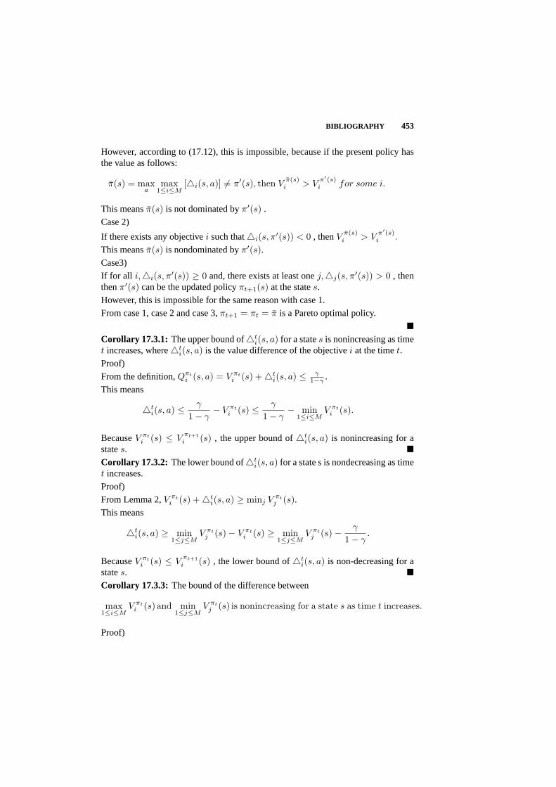
BIBLIOGRAPHY 453
However, according to (17.12), this is impossible, because if the present policy hasthe value as follows:
π(s) = maxa
max1≤i≤M
[4i(s, a)] 6= π′(s), then Vπ(s)i > V
π′(s)i for some i.
This meansπ(s) is not dominated byπ′(s) .
Case 2)
If there exists any objectivei such that4i(s, π′(s)) < 0 , thenVπ(s)i > V
π′(s)i .
This meansπ(s) is nondominated byπ′(s).Case3)
If for all i,4i(s, π′(s)) ≥ 0 and, there exists at least onej,4j(s, π′(s)) > 0 , thenthenπ′(s) can be the updated policyπt+1(s) at the states.
However, this is impossible for the same reason with case 1.
From case 1, case 2 and case 3,πt+1 = πt = π is a Pareto optimal policy.
¥Corollary 17.3.1: The upper bound of4t
i(s, a) for a states is nonincreasing as timet increases, where4t
i(s, a) is the value difference of the objectivei at the timet.
Proof)
From the definition,Qπti (s, a) = V πt
i (s) +4ti(s, a) ≤ γ
1−γ .
This means
4ti(s, a) ≤ γ
1− γ− V πt
i (s) ≤ γ
1− γ− min
1≤i≤MV πt
i (s).
BecauseV πti (s) ≤ V
πt+1i (s) , the upper bound of4t
i(s, a) is nonincreasing for astates. ¥Corollary 17.3.2: The lower bound of4t
i(s, a) for a state s is nondecreasing as timet increases.
Proof)
From Lemma 2,V πti (s) +4t
i(s, a) ≥ minj V πtj (s).
This means
4ti(s, a) ≥ min
1≤j≤MV πt
j (s)− V πti (s) ≥ min
1≤j≤MV πt
j (s)− γ
1− γ.
BecauseV πti (s) ≤ V
πt+1i (s) , the lower bound of4t
i(s, a) is non-decreasing for astates. ¥Corollary 17.3.3: The bound of the difference between
max1≤i≤M
V πti (s) and min
1≤j≤MV πt
j (s) is nonincreasing for a state s as time t increases.
Proof)

454 BIBLIOGRAPHY
Let
di = V πti (s)− min
1≤j≤MV πt
j (s), j = 1, · · · ,M.
Because
di = V πti (s)− min
1≤j≤MV πt
j (s) ≥ 0, 0 ≤ V πti (s) ≤ γ
1− γ,
then
γ
1− γ− min
1≤j≤MV πt
j (s) ≥ − max1≤i≤M
V πti (s)− min
1≤j≤MV πt
j (s) ≥ di ≥ 0 (17.48)
As one can see from (17.48), the upper bound ofdi is nonincreasing for a states,becauseV πt
i (s) ≤ Vπt+1i (s).
¥

18 Adaptive Critic Based NeuralNetwork for Control-ConstrainedAgile Missile
S. N. BALAKRISHNAN and DONGCHEN HAN
University of Missouri-Rolla
Editor’s Summary: This chapter uses the adaptive critic approach, which wasintroduced in Chapters 3 and 4, to steer an agile missile with bounds on the angleof attack (control variable) from various initial Mach numbers to a given final Machnumber in minimum time while completely reversing its flight path angle. While atypical adaptive critic consists of a critic and controller, the agile missile problemneeds chunking in terms of the independent control variable and therefore, cascadesof critics and controllers. Detailed derivations of equations and conditions on theconstraint boundary are provided. For numerical experiments, the authors considervertical plane scenarios. Numerical results demonstrate some attractive features ofthe adaptive critic approach and show that this formulation works very well in guidingthe missile to its final conditions for this state constrained optimization problem froman envelope of initial conditions.
18.1 INTRODUCTION
In order to explore and extend the range of operations of air-to-air missiles, therehave been studies in recent years with a completely new concept. Launch the missileas usual from an aircraft but find a control that can guide it to intercept a target evenif it is in the rear hemisphere (see Figure 18.1).
The best emerging alternative to execute this task is to use the aerodynamics andthrust to turn around the initial flight path angle of zero to a final flight path angleof 180 degrees. (Every missile-target scenario can be considered as a subset of thisset of extremes in the flightpath angle.) In this study, the problem is made morepractical by limiting the missile to fly below a certain value of angle of attack. Thissort of constraint is usually imposed in a problem due to the controller (actuator) or
455

456 ADAPTIVE CRITIC BASED NN FOR CONTROL-CONSTRAINED AGILE MISSILE
X
Y
Z
Fig. 18.1 Agile Missile Trajectory.
structural load limits etc. In calculus of variations, this problem is called the ’freefinal time and control-constrained’ and it is very difficult to obtain solutions for itwhen the initial flight envelope is large. To our knowledge, there is no publicationdealing with this difficult problem except with a single set of initial conditions.
In this study, however, solutions are obtained through the framework of optimalcontrol. Optimization has been a field of interest to mathematicians, scientists andengineers for a long time. For optimal solutions which encompass perturbationsto the assumed initial conditions or a family of initial conditions, a control systemdesigner can use ’neighboring optimal’ control [1] or dynamic programming [1].Neighboring optimal control allows pointwise solutions to a (optimal) two-pointboundary value problem to be used with a linearized approximation over a range ofinitial conditions. However, the neighboring optimal solution can fail outside thedomain of validity of the linearization process. Dynamic programming can handlea family of initial conditions for linear as well as nonlinear problems. The usualmethod of solution, however, is computation-intensive. Furthermore, the solution isnot generally available as a feedback that can be implemented in practice [2, 3].
Werbos citebala:10 proposed a means to get around this numerical complexity byusing ’approximate dynamic programming’(ADP) formulations. His methods ap-proximate the original problem by a discrete formulation. The solution to the ADPformulation is obtained through the two-neural network adaptive critic approach.This ADP process, through the nonlinear function approximation capabilities of neu-ral networks, overcomes the computational complexity that plagued the dynamicprogramming formulation of optimal control problems. More important, this solu-tion can be implemented on-line, since the control computation requires only a fewmultiplications of the network weights which are trained off-line. This techniquewas used by Balakrishnan to solve an aircraft control problem. Several authors haveused neural networks to “optimally” solve nonlinear control problems [4, 5, 6]. Forexample, Kim and Calise [7] have proposed a neural network based control correctionbased on Lyapunov theory. A major difference between their approach and this studyis that the development of guidance law/control is based on optimal control; hence,it is stabilizing and at the same time minimizing a cost.
PROBLEM FORMULATION AND SOLUTION DEVELOPMENT 457
In this study, a cascade of dual neural networks is used as a framework for thesolutions of linear as well as nonlinear,finite-timeoptimal control problems witha special application to an agile missile. In a typical adaptive critic design, thecontroller output does not depend the current time but only the current states; inthis problem, by contrast, the controller output has to be different for the samevalues of the state since the time left to complete the task plays a role in how muchcontrol has to be used. Hence, a cascade of controllers is synthesized by ‘chunking’the independent variable. Rest of this paper is organized as follows: Approximatedynamic programming development in the context of a fairly general finite timeoptimal control problem presented in Section 18.2. Hamiltonian corresponding tothe control constraints, features of constrained problems and optimal solutions on theconstraint boundary are also discussed. Equations of motion for the agile missile aregiven in Section 18.3. Neural network solutions to minimum time bounded control ofthe agile missile are also discussed in Section 18.3. In Section 18.4, it is shown how touse the neurocontroller as a feedback controller. Simulation results and conclusionsare presented in Section 18.5 and Section 18.6 respectively.
18.2 PROBLEM FORMULATION AND SOLUTION DEVELOPMENT
18.2.1 Approximate Dynamic Programming
In this section, general development on the optimal control of the nonlinear systemsis presented in an ADP framework. Detailed derivations of these conditions may alsobe found in [6, 10] which are repeated here for the sake of clarity and completeness.The development in this section will subsequently be used in synthesizing the neuralnetworks for optimal control of the agile missile. Note that the neural networksolution consists of two parts-solution when the control constraint is active and asolution when the constraint is not active.
Discrete description of a fairly general system model is given by
xi+1 = fi(xi, ui) (18.1)
wherefi() can be either linear or nonlinear;i indicates the stage . The problem is tofind a control sequenceui to minimize the cost functionJ where
J = φ[xN ] +N−1∑
i=0
Li[xi, ui]. (18.2)
Subject to a control inequality constraint:
C(ui) ≤ 0 (18.3)
In Eq. (18.2),Li() can be a linear or nonlinear function of the states and/or controlandφ() can be a linear or nonlinear function of terminal states.
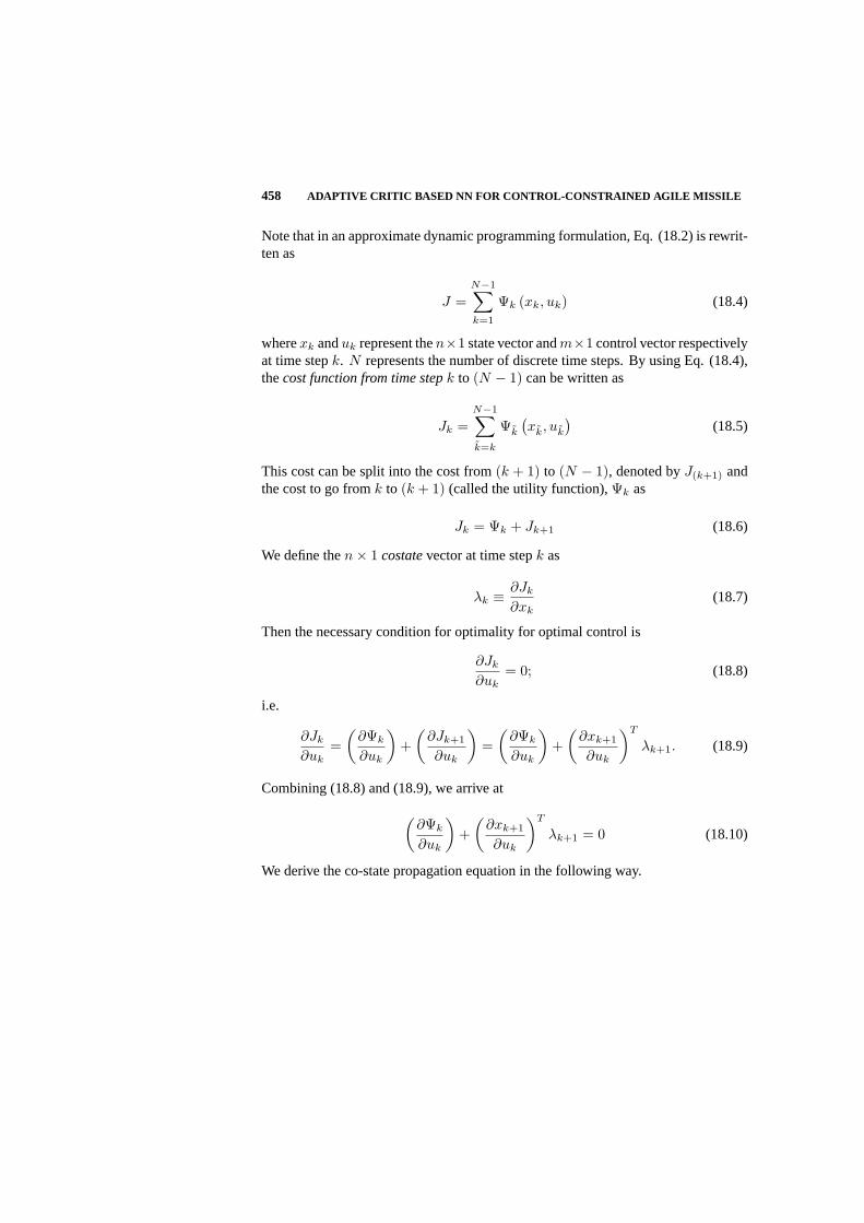
458 ADAPTIVE CRITIC BASED NN FOR CONTROL-CONSTRAINED AGILE MISSILE
Note that in an approximate dynamic programming formulation, Eq. (18.2) is rewrit-ten as
J =N−1∑
k=1
Ψk (xk, uk) (18.4)
wherexk anduk represent then×1 state vector andm×1 control vector respectivelyat time stepk. N represents the number of discrete time steps. By using Eq. (18.4),thecost function from time stepk to (N − 1) can be written as
Jk =N−1∑
k=k
Ψk
(xk, uk
)(18.5)
This cost can be split into the cost from(k + 1) to (N − 1), denoted byJ(k+1) andthe cost to go fromk to (k + 1) (called the utility function),Ψk as
Jk = Ψk + Jk+1 (18.6)
We define then× 1 costatevector at time stepk as
λk ≡ ∂Jk
∂xk(18.7)
Then the necessary condition for optimality for optimal control is
∂Jk
∂uk= 0; (18.8)
i.e.
∂Jk
∂uk=
(∂Ψk
∂uk
)+
(∂Jk+1
∂uk
)=
(∂Ψk
∂uk
)+
(∂xk+1
∂uk
)T
λk+1. (18.9)
Combining (18.8) and (18.9), we arrive at
(∂Ψk
∂uk
)+
(∂xk+1
∂uk
)T
λk+1 = 0 (18.10)
We derive the co-state propagation equation in the following way.
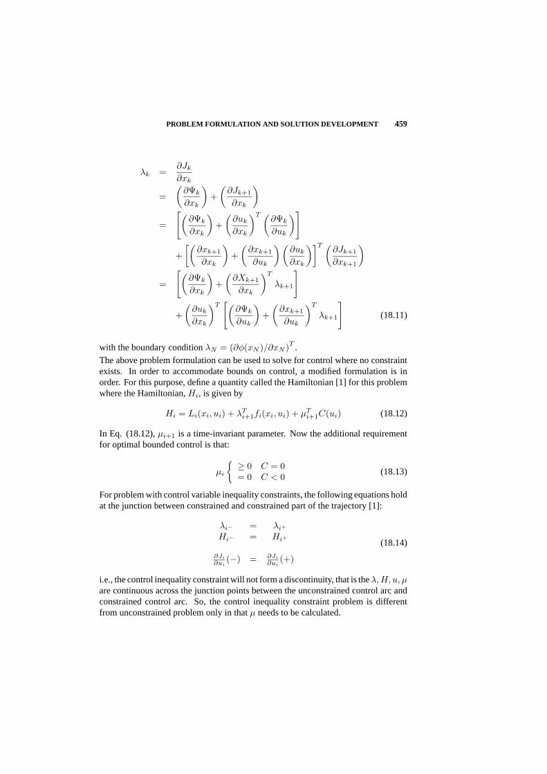
PROBLEM FORMULATION AND SOLUTION DEVELOPMENT 459
λk =∂Jk
∂xk
=(
∂Ψk
∂xk
)+
(∂Jk+1
∂xk
)
=
[(∂Ψk
∂xk
)+
(∂uk
∂xk
)T (∂Ψk
∂uk
)]
+[(
∂xk+1
∂xk
)+
(∂xk+1
∂uk
)(∂uk
∂xk
)]T (∂Jk+1
∂xk+1
)
=
[(∂Ψk
∂xk
)+
(∂Xk+1
∂xk
)T
λk+1
]
+(
∂uk
∂xk
)T[(
∂Ψk
∂uk
)+
(∂xk+1
∂uk
)T
λk+1
](18.11)
with the boundary conditionλN = (∂φ(xN )/∂xN )T .
The above problem formulation can be used to solve for control where no constraintexists. In order to accommodate bounds on control, a modified formulation is inorder. For this purpose, define a quantity called the Hamiltonian [1] for this problemwhere the Hamiltonian,Hi, is given by
Hi = Li(xi, ui) + λTi+1fi(xi, ui) + µT
i+1C(ui) (18.12)
In Eq. (18.12),µi+1 is a time-invariant parameter. Now the additional requirementfor optimal bounded control is that:
µi
≥ 0 C = 0= 0 C < 0 (18.13)
For problem with control variable inequality constraints, the following equations holdat the junction between constrained and constrained part of the trajectory [1]:
λi− = λi+
Hi− = Hi+
∂Ji
∂ui(−) = ∂Ji
∂ui(+)
(18.14)
i.e., the control inequality constraint will not form a discontinuity, that is theλ, H, u, µare continuous across the junction points between the unconstrained control arc andconstrained control arc. So, the control inequality constraint problem is differentfrom unconstrained problem only in thatµ needs to be calculated.

460 ADAPTIVE CRITIC BASED NN FOR CONTROL-CONSTRAINED AGILE MISSILE
For C < 0 (constraint is not active), the constraint associate parameterµi = 0 andEq. (18.10) is used in calculatingui. ForC = 0 (the constraint is active), the controlconstraint equation is used to computeui and Eq. (18.12) along with Eq. (18.10) areused in the computation ofµi .
With control solution described, a systematic process of using the time (or stage)-indexed neural networks to solve for control is developed next. Note that since theterminal conditions are given at the last stage, the solution proceeds backwards.
18.2.2 General Procedure for Finite Time Problems Using Adaptive Critics
For finite time (or finite-horizon) problems, a solution with neural networks evolvesin two stages:
Synthesis of Last Network:
1) Note thatλN =(
∂φ(xN )∂xN
)T
. For various random values ofxN , λN can be
calculated.
2) Use the state-propagation Eq.(18.1) and optimality condition in Eq.(18.10) tocalculateuN−1 for variousxN−1 by randomly selectingxN and the corre-spondingλN from step 1.
3) With uN−1 andλN , calculateλN−1 for variousxN−1 by using the costatepropagation Eq.(18.11).
4) Train two neural networks. For different values ofxN−1, theuN−1 networkoutputsuN−1 and theλN−1 network outputsλN−1. We have optimal controland costates for various values of the state at stage(N − 1) now.
Other Networks:
1) Assume different values of states atxN−2 at stage(N − 2) and pick a randomnetwork (or initialized withuN−1 network) calleduN−2 network to outputuN−2. UseuN−2 andxN−2 in the state propagation equation to getxN−1.Input xN−1 to theλN−1 network to obtainλN−1. UsexN−2 andλN−1 inthe optimality condition in Eq.(18.10) to get targetuN−2. Use this to correcttheuN−2 network. Continue this process until the network weights show littlechanges. ThisuN−2 network yields optimaluN−2.
2) Using randomxN−2, output the controluN−2 from theuN−2 network. UsethesexN−2 anduN−2 to getxN−1 and inputxN−1 to generateλN−1. UsexN−2, uN−2 andλN−1 to obtain optimalλN−2. Train aλN−2 network withxN−2 as input and obtain optimalλN−2 as output.
3) Repeat the last two steps withi = N − 1, N − 2, . . . 0, until uo is obtained.
A schematic of the network development is presented in Figure 18.2.

MINIMUM TIME HEADING REVERSAL PROBLEM IN A VERTICAL PLANE 461
uN-1 uN-2 U0
N-1N-2 0
Fig. 18.2 Schematic of Successive Adaptive Critic Synthesis.
18.3 MINIMUM TIME HEADING REVERSAL PROBLEM IN AVERTICAL PLANE
The equations of motion in a vertical plane are presented and the minimum timeproblem is formulated this section. The main goal of this study is to find the control(angle-of-attack) history to minimize the time taken by the missile in reversing itsflightpath angle while using an upper bound on the control, angle of attack.. In manyengagements, most of the flight is dominated by two-dimensional motion-either ina horizontal or vertical plane. It should be noted that extension of this method to athree-dimensional engagements is straight-forward.
18.3.1 Equations of Motion of A Missile in a Vertical Plane
The non-dimensional equations of motion of a missile(represented as a point mass)in a vertical plane are:
M ′ = −SwM2CD − sinγ + Twcosα (18.15)
γ′ =1M
[SwM2CL + Twsinα− cosγ
](18.16)
XE = Mcosγ (18.17)
ZE = −Msinγ (18.18)
where prime denotes differentiation with respect to nondimensional time,τ .
The nondimensional parameters used in Eqs. (18.15) - (18.18) are:
τ = g/at; Tw = T/mg; Sw = ρ a2 S/2mg andM = V/a.
In these equations,M is the flight Mach number,γ, the flightpath angle,α, theaerodynamic angle of attack,T , the solid rocket thrust,m, the mass of the missile,S,the reference aerodynamic area,V , the speed of the missile,CL, the lift coefficient,CD, the drag coefficient,g, the acceleration due to gravity,a, the speed of sound,ρ,the atmospheric density, andt is the flight time. Note thatCD andCL are functionsof angle of attack and flight Mach number and a neural network is trained to out putCD andCL with angle of attack and flight Mach number as inputs.XE andZE arethe non dimensional velocities in the horizontal and vertical directions respectively.
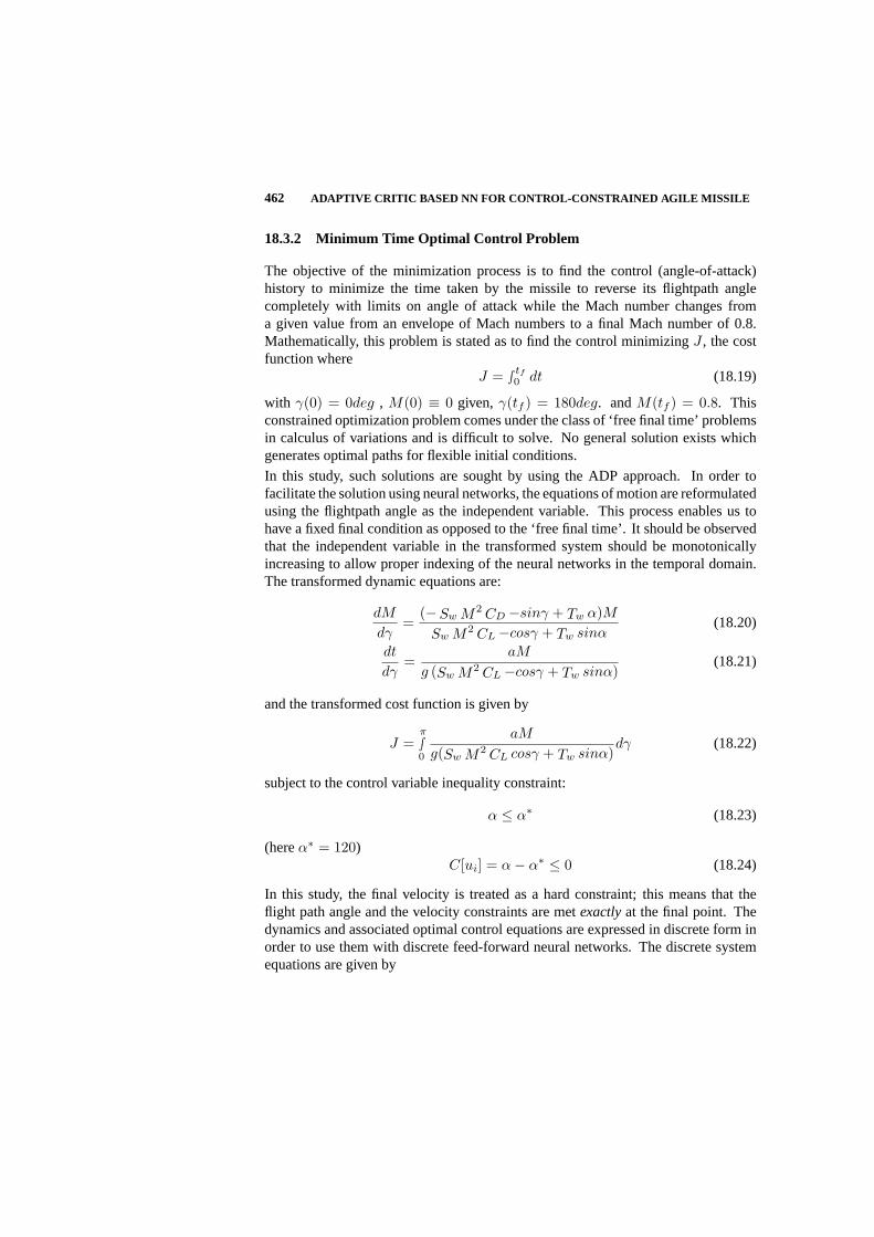
462 ADAPTIVE CRITIC BASED NN FOR CONTROL-CONSTRAINED AGILE MISSILE
18.3.2 Minimum Time Optimal Control Problem
The objective of the minimization process is to find the control (angle-of-attack)history to minimize the time taken by the missile to reverse its flightpath anglecompletely with limits on angle of attack while the Mach number changes froma given value from an envelope of Mach numbers to a final Mach number of 0.8.Mathematically, this problem is stated as to find the control minimizingJ , the costfunction where
J = ∫ tf
0 dt (18.19)
with γ(0) = 0deg , M(0) ≡ 0 given, γ(tf ) = 180deg. andM(tf ) = 0.8. Thisconstrained optimization problem comes under the class of ‘free final time’ problemsin calculus of variations and is difficult to solve. No general solution exists whichgenerates optimal paths for flexible initial conditions.
In this study, such solutions are sought by using the ADP approach. In order tofacilitate the solution using neural networks, the equations of motion are reformulatedusing the flightpath angle as the independent variable. This process enables us tohave a fixed final condition as opposed to the ‘free final time’. It should be observedthat the independent variable in the transformed system should be monotonicallyincreasing to allow proper indexing of the neural networks in the temporal domain.The transformed dynamic equations are:
dM
dγ=
(−Sw M2 CD −sinγ + Tw α)MSw M2 CL−cosγ + Tw sinα
(18.20)
dt
dγ=
aM
g (Sw M2 CL−cosγ + Tw sinα)(18.21)
and the transformed cost function is given by
J =π
∫0
aM
g(Sw M2 CL cosγ + Tw sinα)dγ (18.22)
subject to the control variable inequality constraint:
α ≤ α∗ (18.23)
(hereα∗ = 120)C[ui] = α− α∗ ≤ 0 (18.24)
In this study, the final velocity is treated as a hard constraint; this means that theflight path angle and the velocity constraints are metexactlyat the final point. Thedynamics and associated optimal control equations are expressed in discrete form inorder to use them with discrete feed-forward neural networks. The discrete systemequations are given by

MINIMUM TIME HEADING REVERSAL PROBLEM IN A VERTICAL PLANE 463
Mk+1 = Mk +
(−SwM2kCDk − sin γk + Twk cos αk
)Mk
SwM2kCLk − cos γk + Twk sinαk
· δγk
tk+1 = tk +aMk
δγk
g (SwM2kCLk − cos γk + Twk sin αk)
. (18.25)
The discrete Hamiltonian is
Hk =(
dt
dγ
)
k
δγk + λk+1Mk+1 + µk+1C[ui+1]
=aMk δγk
g (Sw M2k CLk − cos γk + Twk sin αk)
(18.26)
+ λk+1
[Mk +
(−Sw Mk CDk − sin γk + Twk cosαk)Mk δγk
Sw M2k CLk − cos γk + Twk sin αk
]
+ µk+1 αk
The denominator of the first term on the right hand side sans g appears in manyexpressions and its derivatives are needed. Hence, for convenience, we define
den = Sw Mk CLk − cos γk +Twk sin αk (18.27)∂den
∂ αk= Sw M
2k
∂ CLk
∂ αk+ Twk cos αk (18.28)
∂den
∂ Mk= 2 Sw M
2k CLk + Sw M
2k
∂ CLk
∂ Mk(18.29)
Derivatives of lift and drag coefficients with respect to the angle of attack and theMach number are obtained from a neural network which stores these coefficients.The costate equation is
λk =a · δγk
g · den− a Mk δγk
g · den2 · ∂den
∂ Mk(18.30)
+ λk+1 ·δγk
(−3 Sw M2
k CDk −Sw M3k
∂ CDk
∂ Mk− sin γk +Twk cos αk
)
den
λk+1 + λk+1 ·δγk
(Sw M2
k CDk + sin γk −Twk cos αk
) ·Mk
den2 · ∂den
∂ Mk
Optimality condition is obtained in an expanded form as

464 ADAPTIVE CRITIC BASED NN FOR CONTROL-CONSTRAINED AGILE MISSILE
a
g· ∂den
∂ αk+ λk+1 ·
(SwM2
k
∂ CDk
∂ αk+ Twk sin αk
)· den
+λk+1
(−Sw M2k CDk − sin λk + Twk cosαk
) · ∂den
∂ αk+ µk+1 = 0 (18.31)
18.3.3 Development of Neural Network Solutions
Neural network synthesis for a finite time problem consists of two steps. It beginsfrom the last stage and proceeds backwards. Note thatφ(·) is zero in this formulation;however, the final state,MN is specified.
18.3.3.1 Last Network Synthesis
1. Final Mach number,MN , is fixed at 0.8. For random values ofMN−1, calculateαN−1 from the state propagation equation.
2. Use optimality condition to solve for appropriateλN .
3. From the costate propagation equation, calculateλN−1.
4. Train two neural networks: TheαN−1 network outputsαN−1 for differentvalues ofMN−1 and theλN−1 network outputsλN−1 for different values ofMN−1. We have optimalαN−1 andλN−1 now.
18.3.3.2 Synthesis of Other Networks
1. Assume different values ofMN−2 and use a random neural network (or initial-ized withαN−1 network) calledαN−2 network to outputαN−2. UseMN−2
andαN−2 to obtainMN−1. InputMN−1 to λN−1 network to getλN−1.
UseMN−2, λN−1 in the optimality equation to solve forαN−2. Use thisαN−2
to correct the network. Continue this process untilαN−2 network converges.ThisαN−2 network yields optimalαN−2.
2. Using randomMN−2 into αN−2 network obtains optimal∀N−2. UseMN−2
andαN−2 to obtainMN−1 and input toλN−1 network to generateλN−1.UseMN−2, αN−2 , andλN−1 in costate equation to obtain optimalλN−2.TrainλN−2 network withMN−2 as input. We haveλN−2 network that yieldsoptimalλN−2.
3. Repeat steps 1 and 2 withk = N − 1, N − 2, . . . , 0, until we getαo .
A schematic of the network development is presented in Figure 18.2.
Note that this procedure sweeps backwards [11]. At each step, we check whether theangle of attack constraint is violated. If it is, then the control target is made equal thelimit value. Note that theµ value needs not to be calculated since it doesn’t affectthe procedure.
USE OF NETWORKS IN REAL-TIME AS FEEDBACK CONTROL 465
18.4 USE OF NETWORKS IN REAL-TIME AS FEEDBACK CONTROL
Assume anyM0 [within the trained range]. Useα0 neural network to find optimalαand integrate untilγ1 for α1 network is reached; use theM1 values to findα1 fromtheα1 neural network and integrate untilγ2 is reached, and so on, untilγf is reached.
Note that the forward integration is done in terms of time (which is available as anincidental variable as a function of the flightpath angle Eq.(18.25). As a result, eventhough the network synthesis is done off-line, the control is a feedback process basedon current states.
18.5 NUMERICAL RESULTS
Representative numerical results with the agile missile simulation are provided in thissection. Tables of aerodynamic data ofCL andCD variations with Mach numbersand angle of attack were provided in [12, 13]. Outputs from the neural networkmodels of these tables were used for extracting these coefficients at different anglesof attack. These data allow estimation of the aerodynamic coefficients at unusuallyhigh angles of attack that are encountered in such rear hemisphere flights. All theneural networks in this study are feedforward networks. A feedforward networkwasselected in order to facilitate numerical derivatives of the outputs with respect tothe inputs. Each network has a three-layered structure with the first layer having atangent sigmoidal activation function, the second layer having a logarithmic sigmoidalactivation function and the third layer having a unit gain. Each layer consists of nineneurons. The results proved that the choices were adequate. There was no effort tooptimize the structure of networks in this study. A Levenberg-Marquardt method isused to train the networks. Based on the authors’ experience, many other trainingmethods could have been applied, equally well.
The control variable inequality constraint is chosen such that the angle of attack,α ≤ 120deg. This value does not have any particular meaning, it is only chosen fortesting the adaptive critic neural network technique for control constrained problems.The solution process as pointed out earlier proceeds backward from the last step.At each step, the control value was checked to see whether it exceeded the limit.Otherwise, the solution marched on as if the problem is unconstrained. Thirty sevennetworks were needed to implement this optimal process. Time histories of Machnumber, costates, angle of attack and the flightpath angle with an initial Mach numberequal to 0.8 are presented in Figure 18.3.
Note that all these results are forward integration in terms of time. From Figure18.3(a), it is clear that the ADP formulation met the final Mach number constraintexactly; the corresponding costate history is given in Figure 18.3(b). From Figure18.3(c), it can be seen that the bound on control input was met exactly as well. Figure18.3(d), presents the reversal of the flight path angle that was the objective of theproblem. The real advantage of using the adaptive critic approach is clear from theMach number history with flightpath angle in Figure 18.4(a).

466 ADAPTIVE CRITIC BASED NN FOR CONTROL-CONSTRAINED AGILE MISSILE
(a) Mach No. History (b) Costate History
(c) Angle of Attack History (d) Flightpath Angle History
Fig. 18.3 Time histories of Mach number, costates, angle of attack and the flightpath anglewith M0 = 0.8, Mf = 0.8.
For each trajectory with an initial Mach number varying from 0.6 to 0.8, the finalMach number is 0.8. That is, the same cascade of neurocontroller is used to generateoptimal control for an envelope of initial conditions. In order to compare the controlconstrained solution with the unconstrained solution, we also plot the Mach numbervariations with the flight path angle and the angle of attack variations for boththe unconstrained and control constrained problem in Figures 18.4(b) and 18.4(c)respectively. From the Mach number history, we can see that the Mach numbersfor the constrained problem are slightly higher than its corresponding part withoutthe constraint. This is to be expected since smaller angle of attacks result in higherspeeds. Further numerical experiments were conducted to test the robustness of thecontroller. Six controller in the mid-flightpath angle region (which means that someof the controls are held constant for longer periods) were removed and the trajectorieswere generated by using the remaining controllers. Mach number histories and theangle of attack of a 37-networks controller and a 31-networks controller are presentedin Figure 18.4(a) and Figure 18.5(b).

NUMERICAL RESULTS 467
(a) Mach No. History vs. Flightpath Angle (b) Mach No. Comparison (Bounded Control v.s.
(M0 varies from 0.6 to 0.8 andMf = 0.8) Unconstraint Problem,M0 = 0.8, Mf = 0.8)
(c) Control History (Bounded Control v.s. Unconstraint Problem,M0 = 0.8, Mf = 0.8)
Fig. 18.4 Mach Number and Control Histories.
(a) Mach No. History (b) Angle of Attack History
Fig. 18.5 Mach Number and Angle of Attack Histories (M0 = 0.8, Mf = 0.8).

468 ADAPTIVE CRITIC BASED NN FOR CONTROL-CONSTRAINED AGILE MISSILE
From the simulation results, it can be seen that even though the trajectory is lessoptimal, the lesser network configuration still delivers the missile at the exact finalMach number of 0.8. Note that if further compactness is required, we can reduce thecontroller to be embedded in a single network by adding the flight path angle as anextra indexing input.
18.6 CONCLUSIONS
An approximate dynamic programming based formulation with an adaptive criticimplementation was used to find optimal solution for a ‘bounded control, free finaltime’ problem associated with an agile missile control. The neural network con-trollers are able to provide (near) optimal control to the missile from an envelopeof initial Mach numbers to a fixed final Mach number of 0.8 in minimum time. Anadded advantage in using these neurocontrollers is that they provide minimum timesolutions even when we change the initial flight path angle from zero to any non zero(positive) value. To our knowledge, there has been no one tool (other than dynamicprogramming) which provides such solutions.
Acknowledgments
This research was supported partially by an Air Force Grant #F08630-96-1-0001 and a NationalScience Foundation Grant #ECS-9976588.
Bibliography
1. A. E. Bryson, Y. Ho, “Applied Optimal Control, Hemisphere Publishing Co.,”pp. 128-211, 1975.
2. A. Weinreb, A.E. Bryson, “Optimal Control System with Hard Control Bounds,”IEEE Trans. on Automatic Control,vol .30, No. 11, pp1135-1138, 1985.
3. B. Wie, C.H. Chuang and J. Sunkel, “Minimum-Time Pointing Control of Two-Link Manipulator,”Journal of Guidance, Control and Dynamics,Vol. 13, No. 5,pp. 867-872, September-October., 1990.
4. K.J. Hunt, “Neural Networks for Controller Systems, A Survey,”Automatica,vol. 28, No. 6, pp. 1083-1112, 1992.
5. D.A. White, D. Sofge,Handbook of Intelligent Control,Van Nostrand Reinhold,Ch. 3,5,8,12,13, 1992.
6. S.N. Balakrishnan, V. Biega, “Adaptive Critic Based Neural Networks for Air-craft Optimal Control,”Journal of Guidance, Control, and Dynamics,vol. 19,no. 4, , pp. 893-898, July - August, 1996.
7. B.S. Kim, A.J. Calise. “Nonlinear Flight Control Using Neural Networks,”AIAAJournal of Guidance, Control, and Dynamics,vol. 20, no. 1, pp. 26-33, 1997.
8. A.G. Barto, R. S. Sutton, and C. W. Anderson, “Neuronlike Adaptive ElementsThat Can Solve Difficult Learning Control Problems,”IEEE Transactions onSystems, Man, and Cybernetics,vol. SMC-13, pp. 834-846, 1983.
9. P.J. Werbos, “Neurocontrol and Supervised Learning; An Overview and Evalu-ation,” Handbook of Intelligent Control,Van Nostrand Reinhold, 1992.
10. P. J. Werbos, “Approximate dynamic programming for real-time control andneural modeling,” D.A. White & D.A. Sofge (Eds.),Handbook of IntelligentControl,Van Nostrand Reinhold, 1992.
11. D. Han, S.N. Balakrishnan, “Adaptive Critic Based Neural Networks for AgileMissile Control,” AIAA Guidance, Navigation, and Control Conference andExhibit,Boston, Massachusetts, pp. 1803-1812, August 10-12, 1998.
469

470 BIBLIOGRAPHY
12. K.D. Burns, and others, “Missile DATCOM,” WL-TR-91-3039.
13. M. Innocenti, “Integrated Approach to Guidance and Control of AlternateControl Technology Flight Vehicle,” Annual Technical Report, prepared un-der Grant:F08630-94-1-001 for Department of the Air Force Wright Laboratory,Eglin Air Force Base, 1995.

19 Applications of ApproximateDynamic Programming in PowerSystems Control
GANESH K VENAYAGAMOORTHY and RONALD G HARLEYDONALD C WUNSCHUniversity of Missouri-Rolla Georgia Institute of Technology
Editor’s Summary: This chapter presents application examples in the field of powersystems control using adaptive-critic designs. These adaptive-critic techniques wereintroduced in chapters 3 and 4, but this chapter does contain an in-depth review of thebasic ideas and how they apply to the specific problems examined in this chapter. Theprimary systems examined here are the three-phase micro alternators at the Universityof Natal in Durban, South Africa. The design and training of the procedure for thecritic and action networks are described in detail. Both simulation results and actualhardware implementations are discussed. Detailed results are presented that comparehow different adaptive-critic schemes perform and what type of performance can beexpected with realistic problems. For another discussion about control of realisticpower systems see chapter 23.
19.1 INTRODUCTION
Power system control essentially requires a continuous balance between electricalpower generation and a varying load demand, while maintaining system frequency,voltage levels and the power grid security. However, generator and grid disturbancescan vary between minor and large imbalances in mechanical and electrical generatedpower, while the characteristics of a power system change significantly betweenheavy and light loading conditions, with varying numbers of generator units andtransmission lines in operation at different times. The result is a highly complexand non-linear dynamic electric power grid with many operational levels made upof a wide range of energy sources with many interaction points. As the demand for
471

472 APPLICATIONS OF ADP IN POWER SYSTEMS CONTROL
electric power grows closer to the available sources, the complex systems that ensurethe stability and security of the power grid are pushed closer to their edge.
Synchronous turbogenerators supply most of the electrical energy produced bymankind, and are largely responsible for maintaining the stability and the secu-rity of the electrical network. The effective control of these devices, is therefore,very important. However, a turbogenerator is a highly non-linear, non-stationary,fast acting, multi-input-multi-output (MIMO) device with a wide range of operatingconditions and dynamic characteristics that depend on the power system to whichthe generator is connected too. Conventional automatic voltage regulators (AVRs)and turbine governors are designed based on some linearized power system model,to control the turbogenerator in some optimal fashion around one operating point.At any other operating points the conventional controller technology cannot copewell and the generator performance degrades, thus driving the power system intoundesirable operating states [1]. Additionally, the tuning and integration of the largenumber of control loops typically found in a power station can prove to be a costlyand time-consuming exercise.
Many novel control strategies have been suggested to deal with all these non-idealplant properties as well as aging of plant components. Indeed significant research hasdemonstrated that adaptive control can improve the overall control in turbogeneratorsystems [2, 3], with the objective of extending operational stability margins [2]. Thesetechniques have performed acceptably well in power stations [4], and commercialpower system control manufacturers are beginning to apply self-tuning strategies.
Previous investigations have illustrated that self-tuning schemes will work well ifthe preconditions for stability and convergence are satisfied. However, the nonlinearnature of power systems implies that the estimated linear models are only validfor a small region about a given operating point. In practice, however, a powersystem is frequently subjected to various disturbances such as tap-changing, line andload switching and occasional major disturbances such as short circuits or lightningsurges. All of these may cause excessive variations in plant outputs, leading to abruptchanges in operating conditions, and possibly hunting of the generators. Therefore,if a self-tuning controller is to work safely in practice, it must be reliable and robust.This can be very complex and unwieldy, with expert systems being suggested tofulfill this role [5].
Most adaptive control algorithms use linear models [6] with certain assumptionsof types of noise and possible disturbances. Moreover, for the design of adaptivecontrollers, it has to be assumed that the number of system inputs equals the numberof system outputs. Where necessary this is achieved by using a transformation toreduce the dimensions of the output space, with the drawback that this degradesthe description of the system dynamics. While this is possible for SMIB systems,it becomes unwieldy and almost impossible in large multi-machine power systems.Consequently, the issues of unmodeled dynamics and robustness arise in practicalapplications of these adaptive control algorithms. To allow for all these uncertainties,the traditional controllers are typically designed with large safety margins. In theera of a deregulated electricity industry, and an emphasis on competitive pricing, it

INTRODUCTION 473
will become necessary to reduce these safety margins as much as possible while stillmaintaining a reliable service.
One of the most important problems arising from large-scale electric power systeminterconnection is the low frequency oscillation [7]. Power System Stabilizers (PSSs)are used to damp such oscillations, but the particular position and transfer functionof a PSS is not a simple decision and is usually also based on some linearized systemmodel, as initially proposed by deMello and Concordia [8] based on the basis ofthe single-machine-infinite-bus (SMIB) linearized model. A practical PSS must berobust over a wide range of operating conditions and capable of damping local,intra-area and inter-area system modes [9, 10]. The participation of the generatorsin the different modes of the oscillation depends on the location of the generatorsin the system; some may participate in one mode only and others in more than one[11]. From this perspective, the conventional PSS design approach based on a SMIBlinearized model in the normal operating condition has some drawbacks:
(a) There are uncertainties in the linearized model resulting from the variation inthe operating condition, since the linearization coefficients are derived typicallyat some nominal operating condition.
(b) To implement the PSS for a multimachine power system, its parameters needto be tuned to coordinate with machines and utilities.
Consequently, a realistic solution for stabilizing the low frequency oscillations of amultimachine system is a stabilizer designed from a nonlinear multimachine model inthe first place. Difficulties in a PSS design come from the handling of nonlinearitiesand interactions among generators. During the low frequency oscillation, the rotoroscillates due to the imbalance between mechanical and electrical powers. Thus,handling the nonlinear power flow properly is the key to the PSS design for amultimachine power system. Unfortunately, it is not that simple to handle thenonlinear interaction variables by conventional analytical methods.
In recent years, renewed interest has been shown in power systems control usingnonlinear control theory, particularly to improve system transient stability [12, 13].Instead of using an approximate linear model, as in the design of the conventionalpower system stabilizer, nonlinear models are used and nonlinear feedback lineariza-tion techniques are employed on the power system models, thereby alleviating theoperating point dependent nature of the linear designs. Nonlinear controllers signifi-cantly improve the power system’s transient stability. However, nonlinear controllershave a more complicated structure and are difficult to implement relative to linearcontrollers. In addition, feedback linearization methods require exact system param-eters to cancel the inherent system nonlinearities, and this contributes further to thecomplexity of stability analysis. The design of decentralized linear controllers toenhance the stability of interconnected nonlinear power systems within the wholeoperating region remains a challenging task [14].
However, the use of Computational Intelligence, especially Artificial Neural Net-works (ANNs), offers a possibility to overcome the above-mentioned challenges and

474 APPLICATIONS OF ADP IN POWER SYSTEMS CONTROL
problems of conventional analytic methods. ANNs are good at identifying and con-trolling nonlinear systems [15, 16]. They are suitable for multi-variable applications,where they can easily identify the interactions between the system’s inputs and out-puts. It has been shown that a Multilayer Perceptron (MLP) neural network usingdeviation signals (for example, deviation of terminal voltage from its steady value)as inputs, can identify [17] the complex and nonlinear dynamics of a single machineinfinite bus configuration, with sufficient accuracy, and this information can then beused to design a nonlinear controller which will yield an optimal dynamic systemresponse irrespective of the load and system configurations.
Previous publications have reported on the different aspects of neural network basedcontrol of generators. However, these neurocontrollers require continual onlinetraining of their neural networks after commissioning [18]. In most of the aboveresults, an ANN is trained to approximate various nonlinear functions in the nonlinearsystem. The information is then used to adapt an ANN controller. Since an ANNidentifier is only an approximation to the underlying nonlinear system, there is alwaysresidual error between the true plant and the ANN model of the plant. Stability issuesarise when the ANN identifier is continually trained online and simultaneously usedto control the system. Furthermore, to update weights of the ANN identifier online,gradient descent algorithms are commonly used. However, it is well known inadaptive control that a brute force correction of controller parameters, based onthe gradients of output errors, can result in instability even for some classes oflinear systems [19, 20]. Hence, to avoid the possibility of instability during onlineadaptation, some researchers proposed using ANNs such as radial basis functions,where variable network parameters occur linearly in the network outputs, such thata stable updating rule can be obtained [21]. To date, the development of nonlinearcontrol using ANNs is similar to that of linear adaptive control because the ANNsare used only in linearized regions. Unfortunately, unlike linear adaptive control,where a general controller structure to stabilize a system can be obtained with onlythe knowledge of relative degrees, stabilizing controllers for nonlinear systems aredifficult to design. As a result, most research on ANN based controllers has focusedon nonlinear systems, whose stabilizing controllers are readily available once someunknown nonlinear parts are identified, such as
xn = f(xn−1, ..., x) + bu (19.1)
with full state feedback, wheref is to be estimated by an ANN. Even though somemethods have been suggested for using ANNs in the context of a general controllerstructure [22, 23], the stability implication of updating a network online is unknown.Furthermore, since an ANN controller can have many weights, it is questionablewhether the network can converge fast enough to achieve good performance. Besides,in closed loop control systems with relatively short time constants, the computationaltime required by frequent online training could become the factor that limits themaximum bandwidth of the controller.
Adaptive critic designs (ACDs) are neural network designs capable of optimizationover time, under conditions of noise and uncertainty. This family of ACDs is an ad-

ADAPTIVE CRITIC DESIGNS AND APPROXIMATE DYNAMIC PROGRAMMING 475
dition to other existing neural network based techniques for control and optimization[49]. There are considered to be the most powerful and complicated designs.
This chapter presents work by the authors [24, 25, 26] based on the adaptive critic’stechnique for designing a turbogenerator neurocontroller, which overcomes the riskof instability [27], the problem of residual error in the system identification [28], inputuncertainties [29], and the computational load of online training. The neurocontrolleraugments/replaces the conventional automatic voltage regulator and turbine governor,and is trained in an offline mode prior to commissioning. Two different types ofAdaptive Critics are discussed, namely the Heuristic Dynamic Programming (HDP)type and the Dual Heuristic programming (DHP) type. Results are presented for asingle-machine-infinite-bus, as well as for a multimachine power system, showingthat the DHP neurocontroller produces the best results in comparison to the HDPneurocontroller and conventional controllers even with the inclusion of a powersystem stabilizer.
Section 19.2 of this chapter describes adaptive critic designs and approximate dy-namic programming. The mathematical equations are given for the HDP and DHPdesigns. Section 19.3 describes the general training procedure for the Critic and Ac-tion networks. Section 19.4 describes the power system models studied with adaptivecritic designs. Section 19.5 presents some simulation and hardware implementationresults on the single machine and multimachine power systems.
19.2 ADAPTIVE CRITIC DESIGNS AND APPROXIMATE DYNAMICPROGRAMMING
19.2.1 Background
The adaptive critic designs (ACDs) are neural network designs capable of optimiza-tion over time under conditions of noise and uncertainty. The simplest adaptivecritic designs learn slowly on large problems but they are successful on many realworld difficult small problems. Complex adaptive critics may seem breathtaking, atfirst, but they are the only design approach that shows potential of replicating criticalaspects of human intelligence: ability to cope with a large number of variables inparallel, in real time, in a noisy nonlinear non-stationary environment.
A family of ACDs was proposed by Werbos [32] as a new optimization techniquecombining concepts of reinforcement learning and approximate dynamic program-ming. For a given series of control actions that must be taken sequentially, and notknowing the effect of these actions until the end of the sequence, it is impossible todesign an optimal controller using the traditional supervised learning neural network.The adaptive critic method determines optimal control laws for a system by suc-cessively adapting two ANNs, namely anaction neural network(which dispensesthe control signals) and acritic neural network (which ‘learns’ the desired perfor-mance index for some function associated with the performance index). These twoneural networks approximate the Hamilton-Jacobi-Bellman equation associated with

476 APPLICATIONS OF ADP IN POWER SYSTEMS CONTROL
optimal control theory. The adaptation process starts with a non-optimal, arbitrar-ily chosen, control by the action network; the critic network then guides the actionnetwork towards the optimal solution at each successive adaptation. During the adap-tations, neither of the networks need any ‘information’ of an optimal trajectory, onlythe desired cost needs to be known. Furthermore, this method determines optimalcontrol policy for the entire range of initial conditions and needs no external training,unlike other neurocontrollers.
Dynamic programming prescribes a search which tracks backward from the final step,retaining in memory all suboptimal paths from any given point to the finish, until thestarting point is reached. The result of this is that the procedure is too computationallyexpensive for most real problems. In supervised learning, an ANN training algorithmutilizes a desired output and, having compared it to the actual output, generates anerror term to allow the network to learn. The backpropagation algorithm is typicallyused to obtain the necessary derivatives of the error term with respect to the trainingparameters and/or the inputs of the network. However, backpropagation can be linkedto reinforcement learning via the critic network which has certain desirable attributes.
The technique of using a critic, removes the learning process one step from the controlnetwork (traditionally called the “action network” or “actor” in ACD literature), sothe desired trajectory is not necessary. The critic network learns to approximatethe cost-to-goor strategic utility function (the functionJ of Bellman’s equation indynamic programming) and uses the output of the action network as one of its inputs,directly or indirectly.
In the Dynamic Programming, or Markov Decision Process (MDP), Literature, prob-lems are described in terms of five essential characteristics:
• Epochs
• States
• Actions
• Rewards
• Transition probabilities.
Most of the literature has focused on finite state spaces, where states are knownwith certainty. Actions may have probabilistic rules associated with them, andrewards and (obviously) transition probabilities may also be nondeterministic. Recentliterature has addressed the extension to where states are also nondeterministic.These are known as Partially Observable Markov Decision Processes (POMDP’s).It is straightforward to show that a POMDP can be transformed to a regular MDPwith continuously-valued state variables [33]. Since Adaptive Critics typically havebeen used in control problems with continuous-valued state spaces, they trivially areapplicable to POMDP’s. This observation, by itself, is sufficient reason for the familyof Adaptive Critic approaches to be known and utilized outside the confines of theIntelligent Control community.
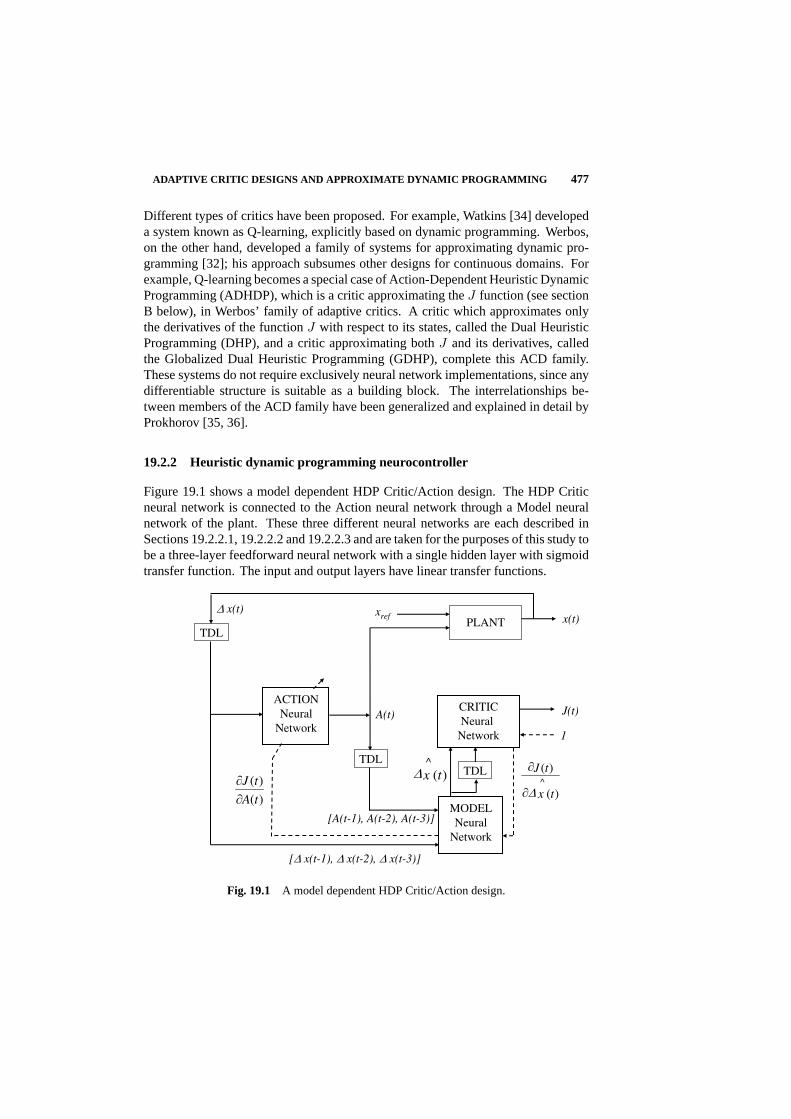
ADAPTIVE CRITIC DESIGNS AND APPROXIMATE DYNAMIC PROGRAMMING 477
Different types of critics have been proposed. For example, Watkins [34] developeda system known as Q-learning, explicitly based on dynamic programming. Werbos,on the other hand, developed a family of systems for approximating dynamic pro-gramming [32]; his approach subsumes other designs for continuous domains. Forexample, Q-learning becomes a special case of Action-Dependent Heuristic DynamicProgramming (ADHDP), which is a critic approximating theJ function (see sectionB below), in Werbos’ family of adaptive critics. A critic which approximates onlythe derivatives of the functionJ with respect to its states, called the Dual HeuristicProgramming (DHP), and a critic approximating bothJ and its derivatives, calledthe Globalized Dual Heuristic Programming (GDHP), complete this ACD family.These systems do not require exclusively neural network implementations, since anydifferentiable structure is suitable as a building block. The interrelationships be-tween members of the ACD family have been generalized and explained in detail byProkhorov [35, 36].
19.2.2 Heuristic dynamic programming neurocontroller
Figure 19.1 shows a model dependent HDP Critic/Action design. The HDP Criticneural network is connected to the Action neural network through a Model neuralnetwork of the plant. These three different neural networks are each described inSections 19.2.2.1, 19.2.2.2 and 19.2.2.3 and are taken for the purposes of this study tobe a three-layer feedforward neural network with a single hidden layer with sigmoidtransfer function. The input and output layers have linear transfer functions.
ACTION
Neural
Network
CRITIC
Neural
Network
J(t)
1
PLANT
MODEL
Neural
Network
TDL
TDL
A(t)
xref x(t)x(t)
)(
)(
tA
tJTDL
[A(t-1), A(t-2), A(t-3)]
[ x(t-1), x(t-2), x(t-3)]
)(
)(^
tx
tJ)(
^
tx
Fig. 19.1 A model dependent HDP Critic/Action design.

478 APPLICATIONS OF ADP IN POWER SYSTEMS CONTROL
19.2.2.1 Model neural networkFor model dependent designs it is assumed that there exists a Model neural network
which is able to predict the states/outputsx(t + 1), of the plant at timet + 1, givenat timet, the states/outputsx(t) and the action signalsA(t).
x(t + 1) = f(x(t), A(t)) (19.2)
In addition to signals at time t, delayed values of these signals can be used as welldepending of the complexity of the plant dynamics [17]. For the purposes of thisstudy the Model neural network predicts thechangesin the outputs∆x(t + 1), attime t + 1 [17]. In Figure 19.1, the inputs to the Model network are time-delayedvalues (TDL) of both the plant and the Action network outputs.
A neural network based technique to develop a Model network using supervisedlearning is shown in Figure 19.1 and more details can be found in [15]. The con-ventional static backpropagation algorithm is used in training the neural network.This Model neural network can undergoofflineor online training, as required by theapplication.
PLANTPlant Inputs Plant Outputs
TDLTDL
MODELNeural Network Σ
-
+
error
Fig. 19.2 Development of a neural network model of a plant.
The ACD controllers designed in this study use the model dependent designs. It isimportant for the description of the following sections to mention that the inputs to theModel neural network are the three time delayed values of the Plant and the Actionnetwork outputs (∆x(t − 1), ∆x(t − 2), ∆x(t − 3), A(t − 1), A(t − 2), A(t − 3))(Figure 19.1) in order to predict∆x(t). In other words, a third order neural networkmodel is used. Explicit details on the development of a Model neural network aregiven in [17, 25, 37].
19.2.2.2 Critic neural networkHeuristic Dynamic Programming has a Critic neural network that estimates the
functionJ (cost-to-go) in the Bellman equation of dynamic programming, expressed
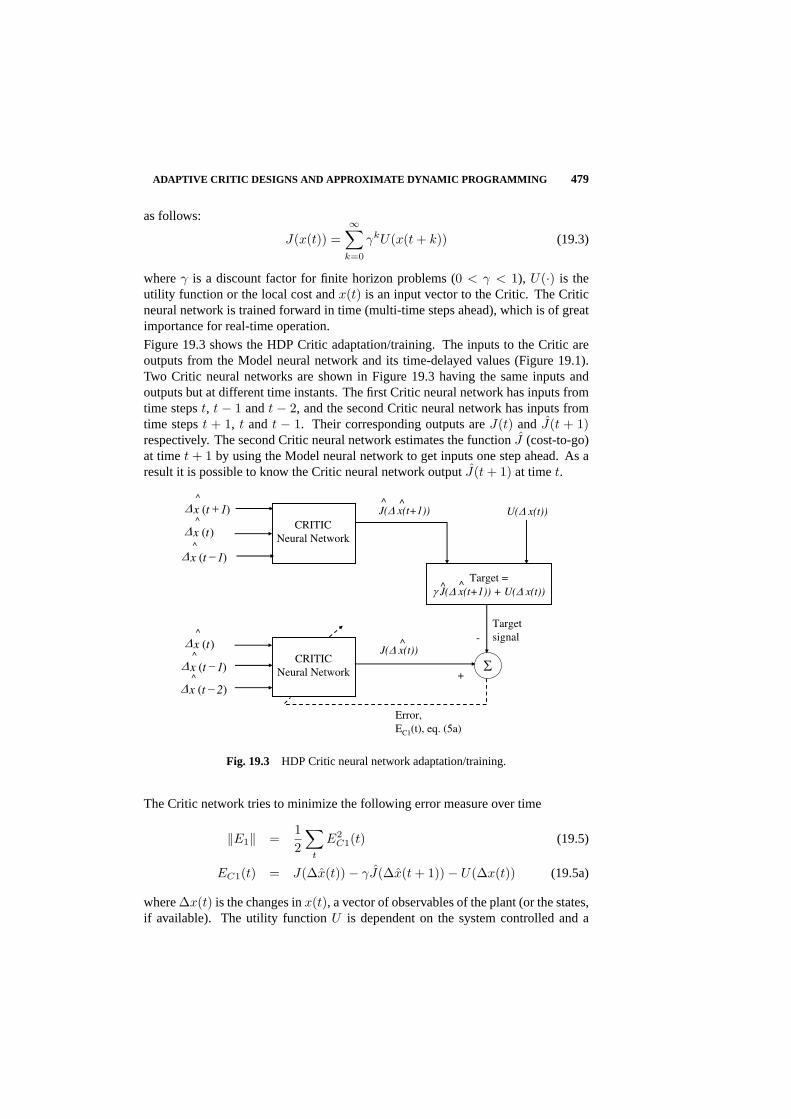
ADAPTIVE CRITIC DESIGNS AND APPROXIMATE DYNAMIC PROGRAMMING 479
as follows:
J(x(t)) =∞∑
k=0
γkU(x(t + k)) (19.3)
whereγ is a discount factor for finite horizon problems (0 < γ < 1), U(·) is theutility function or the local cost andx(t) is an input vector to the Critic. The Criticneural network is trained forward in time (multi-time steps ahead), which is of greatimportance for real-time operation.
Figure 19.3 shows the HDP Critic adaptation/training. The inputs to the Critic areoutputs from the Model neural network and its time-delayed values (Figure 19.1).Two Critic neural networks are shown in Figure 19.3 having the same inputs andoutputs but at different time instants. The first Critic neural network has inputs fromtime stepst, t − 1 andt − 2, and the second Critic neural network has inputs fromtime stepst + 1, t andt − 1. Their corresponding outputs areJ(t) and J(t + 1)respectively. The second Critic neural network estimates the functionJ (cost-to-go)at timet + 1 by using the Model neural network to get inputs one step ahead. As aresult it is possible to know the Critic neural network outputJ(t + 1) at timet.
CRITIC
Neural Network
Target =
J( x(t+1)) + U( x(t))
U( x(t))J( x(t+1))
CRITIC
Neural Network
J( x(t))
Error,
EC1(t), eq. (5a)
+
-
Target
signal
^ ^
^
^ ^
)(^
1tx
)(^
tx
)(^
1tx
)(^
tx
)(^
1tx
)(^
2tx
Fig. 19.3 HDP Critic neural network adaptation/training.
The Critic network tries to minimize the following error measure over time
‖E1‖ =12
∑t
E2C1(t) (19.5)
EC1(t) = J(∆x(t))− γJ(∆x(t + 1))− U(∆x(t)) (19.5a)
where∆x(t) is the changes inx(t), a vector of observables of the plant (or the states,if available). The utility functionU is dependent on the system controlled and a

480 APPLICATIONS OF ADP IN POWER SYSTEMS CONTROL
typical function is given in [25]. It should be noted that only for the purposes ofthis study, changes in the state variables are used rather than state variables. Thenecessary condition for (19.3) to be minimal is given in (19.5b).
12
∂
∂WC1
(E2
C1(t))
=(
EC1∂EC1(t)∂WC1
)= 0 (19.5b)
The weights’ update for the Critic network using the backpropagation algorithm isgiven as follows:
∆WC1 = −ηEC1(t)∂EC1(t)∂WC1
(19.6a)
∆WC1 = −ηJ(∆x(t))− γJ(∆x(t + 1))− U(∆x(t)) × (19.6b)
∂J(∆x(t))− γJ(∆x(t + 1))− U(∆x(t))∂WC1
whereη is a positive learning rate andWC1 are the weights of the Critic neuralnetwork. The same Critic network is shown in two consecutive moments in timein Figure 19.3. The Critic network’s outputJ [∆x(t + 1)] is necessary in order toprovide the training signalγJ [∆x(t + 1)] + U(∆x(t)), which is the desired/targetvalue forJ [∆x(t)].
19.2.2.3 Action neural networkThe objective of the Action neural network in Figure 19.1, is to minimizeJ(∆x(t))
in the immediate future, thereby optimizing the overall cost expressed as a sum of allU(∆x(t)) over the horizon of the problem. This is achieved by training the Actionneural network with an error signal∂J/∂A. The gradient of the cost functionJ , withrespect to the outputsA, of the Action neural network, is obtained by backpropagating∂J/∂J (i.e. the constant 1) through the Critic neural network and then through thepretrained Model neural network to the Action neural network. This gives∂J/∂Aand∂J/∂WA for all the outputs of the Action neural network, and all the Actionneural network’s weightsWA, respectively. The weights’ update in the Action neuralnetwork using backpropagation algorithm is given as follows:
‖E2‖ =12
∑t
E2A1(t) (19.7a)
where
EA1 =∂J(t)∂A(t)
(19.7b)
and∂J(t)∂A(t)
=∂J(t)
∂∆x(t)∂∆x(t)∂A(t)
(19.7c)
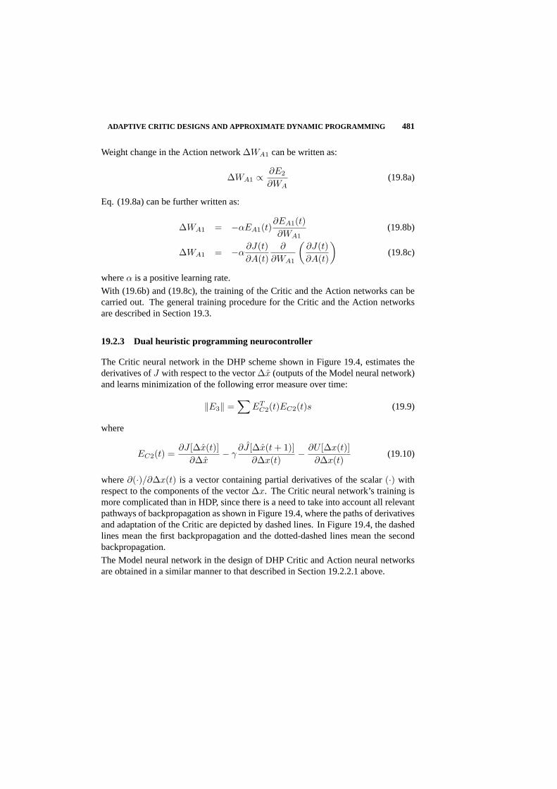
ADAPTIVE CRITIC DESIGNS AND APPROXIMATE DYNAMIC PROGRAMMING 481
Weight change in the Action network∆WA1 can be written as:
∆WA1 ∝ ∂E2
∂WA(19.8a)
Eq. (19.8a) can be further written as:
∆WA1 = −αEA1(t)∂EA1(t)∂WA1
(19.8b)
∆WA1 = −α∂J(t)∂A(t)
∂
∂WA1
(∂J(t)∂A(t)
)(19.8c)
whereα is a positive learning rate.
With (19.6b) and (19.8c), the training of the Critic and the Action networks can becarried out. The general training procedure for the Critic and the Action networksare described in Section 19.3.
19.2.3 Dual heuristic programming neurocontroller
The Critic neural network in the DHP scheme shown in Figure 19.4, estimates thederivatives ofJ with respect to the vector∆x (outputs of the Model neural network)and learns minimization of the following error measure over time:
‖E3‖ =∑
ETC2(t)EC2(t)s (19.9)
where
EC2(t) =∂J [∆x(t)]
∂∆x− γ
∂J [∆x(t + 1)]∂∆x(t)
− ∂U [∆x(t)]∂∆x(t)
(19.10)
where∂(·)/∂∆x(t) is a vector containing partial derivatives of the scalar(·) withrespect to the components of the vector∆x. The Critic neural network’s training ismore complicated than in HDP, since there is a need to take into account all relevantpathways of backpropagation as shown in Figure 19.4, where the paths of derivativesand adaptation of the Critic are depicted by dashed lines. In Figure 19.4, the dashedlines mean the first backpropagation and the dotted-dashed lines mean the secondbackpropagation.
The Model neural network in the design of DHP Critic and Action neural networksare obtained in a similar manner to that described in Section 19.2.2.1 above.

482 APPLICATIONS OF ADP IN POWER SYSTEMS CONTROL
PLANTTDL
MODEL
Neural
Network
#2
CRITIC
Neural
Network
#2
CRITIC
Neural
Network
#1
TDL
MODEL
Neural
Network
#1
xref
x(t)A(t)
(t+1)
TDL
TDL
TDL
TDL
++ +
-
-
-
EC(t)
[ x(t-1), x(t-2), x(t-3)]
[A(t-1), A(t-2), A(t-3)]
ACTION
Neural Network
path 3path 5
path 6
path 4
path 8
path 7 path 9
path 1
path 2
path 10
path 11 path 12
)(
)(
tA
tU
k^
^
^
)(
)(
tx
tU
)(^
1tx
)(^
tx
)(^
1tx
)(
)(
)(
^
1tx
1tJ
1t
)(^
tx
)(^
1tx
)(^
2tx
)(
)(
)(
^
tx
tJ
t
Fig. 19.4 DHP Critic neural network adaptation.
In the DHP scheme, application of the chain rule for derivatives yields:
∂J [∆x(t + 1)]∂∆xj(t)
=n∑
i=1
λi(t + 1)∂∆xi(t + 1)
∂∆xj(t)
+m∑
k=1
n∑
i=1
λi(t + 1)∂∆xi(t + 1)
∂Ak(t)∂Ak(t)∂∆xj(t)
(19.11)
whereλi(t + 1) = ∂J [∆x(t + 1)]/∂∆xi(t + 1), andn, m, j are the numbers ofoutputs of the Model, Action and Critic neural networks respectively. By exploiting(19.11), each of n components of the vectorEC2(t) from (19.10) is determined by
EC2j(t) =∂J [∆x(t)]∂∆xj(t)
− γ∂J [∆x(t + 1)]
∂∆xj(t)
−∂U [∆x(t)]∂∆xj(t)
−m∑
k=1
∂U(t)∂Ak(t)
∂Ak(t)∂∆xj(t)
(19.12)

ADAPTIVE CRITIC DESIGNS AND APPROXIMATE DYNAMIC PROGRAMMING 483
The signals in Figure 19.4 which are labeled with a path number, represent thefollowing:
(i). Path 1 represents the outputs of the plant fed into the Model neural network#2. These outputs are∆x(t), ∆x(t− 1) and∆x(t− 2).
(ii). Path 2 represents the outputs of the Action neural network fed into the Modelneural network #2. These outputs areA(t), A(t− 1) andA(t− 2).
(iii). Path 3 represents the outputs of the plant fed into the Action neural network.These outputs are∆x(t), ∆x(t− 1) and∆x(t− 2).
(iv). Path 4 represents a backpropagated signal of the output of the Critic neuralnetwork #2 through the Model neural network with respect to path 1 inputs.The backpropagated signal on path 4 isn∑
i=1
λi(t + 1)∂∆xi(t+1)∂∆xj(t)
in (19.11).
(v). Path 5 represents a backpropagated signal of the output of the Critic neuralnetwork #2 through the Model neural network with respect to path 2 inputs.The backpropagated signal on path 3 isn∑
i=1
λi(t + 1)∂∆xi(t+1)∂∆Ak(t) in (19.11).
(vi). Path 6 represents a backpropagation output of path 5 signal ((iv) above) withrespect to path 3. The signal on path 6 is∑m
k=1
∑ni=1 λi(t + 1)∂∆xi(t+1)
∂Ak(t) in (19.11).
(vii). Path 7 is the sum of the path 4 and path 6 signals resulting in∂J [∆x(t + 1)]/∂∆xj(t), given in (19.11).
(viii). Path 8 is the backpropagated signal of the term∂U(t)/∂Ak(t) (Figure 19.5)
with respect to path 3 and ism∑
k=1
∂U(t)∂Ak(t)
∂Ak(t)∂∆xj(t)
in (19.12).
(ix). Path 9 is a product of the discount factorγ and the path 7 signal, resulting intermγ∂J [∆x(t + 1)]/∂∆xj(t) in (19.12).
(x). Path 10 represents the output of the Critic neural network #1,∂J [∆x(t)]/∂∆x(t).
(xi). Path 11 represents the term∂U(t)/∂∆x(t) (Figure 19.5).
(xii). Path 12 representsEC2j(t) given in (19.12) and as follows:
Path12 = EC2j(t) = Path10− Path9− Path11− Path8.
The partial derivatives of the utility functionU(t) with respect toAk(t), andx(t),∂U(t)/∂Ak(t) and∂U(t)/∂∆x(t) respectively, are obtained by backpropagating theutility function, U(t) through the Model network as shown in Figure 19.5.

484 APPLICATIONS OF ADP IN POWER SYSTEMS CONTROL
MODEL
Neural
NetworkU(t)
)(
)(
tA
tU
k
)(
)(
tx
tU
Fig. 19.5 Backpropagation ofU(t) through the Model neural network.
The adaptation of the action network in Figure 19.4, is illustrated in Figure 19.6which propagatesλ(t + 1) back through the model network to the action network.The goal of such adaptation can be expressed as follows [35, 36]:
∂U [∆x(t)]∂A(t)
+ γ∂J [∆x(t + 1)]
∂A(t)= 0 ∀t
The error signal for the Action network adaptation is therefore given as follows:
EA2(t) =∂U [∆x(t)]
∂A(t)+ γ
∂J [∆x(t + 1)]∂A(t)
(19.14)
The weights’ update expression [36], when applying backpropagation, is as follows:
∆WA2 = −α
[∂U [∆x(t)]
∂A(t)+ γ
∂J [∆x(t + 1)]∂A(t)
]T∂A(t)∂WA2
(19.15)
whereα is a positive learning rate andWA2 are weights of the DHP Action neuralnetwork.
PLANTTDL
ACTION
Neural
Network
MODEL
Neural
Network
CRITIC
Neural
Network
TDL
xref
x(t)
A(t)
)(
)(
tA
tU
(t+1)
TDL
TDL
++
x(t)
)(
)(
tA
1tJ
EA2(t)
)(
)(
)(
^
1tx
1tJ
1t
)(^
1tx
)(^
tx
)(^
1tx
Fig. 19.6 DHP Action neural network adaptation.

GENERAL TRAINING PROCEDURE FOR CRITIC AND ACTION NETWORKS 485
19.3 GENERAL TRAINING PROCEDURE FOR CRITIC AND ACTIONNETWORKS
The training procedure is that suggested in [36] and it is applicable to any ACD.It consists of two separate training cycles: one for the Critic, and the other for theAction. An important measure is that the Action neural network is pretrained withconventional controllers (Proportional Integral Derivative, PID) controlling the plantin a linear region. The Critic’s adaptation is done initially with the pretrained Actionnetwork, to ensure that the whole system, consisting of the ACD and the plant remainsstable. Then the Action network is trained further while keeping the Critic neuralnetwork weights fixed. This process of training the Critic and the Action one afterthe other, is repeated until an acceptable performance is reached. It is assumed thatthere is no concurrent adaptation of the pretrained Model neural network, andWC isinitialized to small random values.
In the Critic’s training cycle, an incremental optimization of (19.5) and/or (19.9)is carried out using a suitable optimization technique (e.g. backpropagation). Thefollowing operations are repeatedNC times:
1. Initialize t = 0 and∆x(0)
2. Compute the output of the Critic neural network at timet,J(t) or λ(t) = fC(∆x(t),WC)
3. Compute the output of the Action neural network at timet,A(t) = fA(∆x(t),WA)
4. Compute the output of the Model neural network at timet + 1,∆x(t + 1) = fM (∆x(t), A(t), WM )
5. Compute the output of the Critic neural network at timet + 1,J(t + 1) or λ(t + 1) = fC(∆x(t + 1),WC)
6. Compute the Critic neural network error at timet,EC1(t) from (19.5a) orEC2(t) from (19.10).
7. Update the Critic neural network’s weights using the backpropagation algo-rithm.
8. Repeat steps 2 to 7.
The functionsfC(∆x(t),WC), fA(∆x(t),WA) andfM (∆x(t), A(t),WM ) repre-sent the Critic, the Action and the Model neural networks with their weightsWi,respectively.
In the Action neural network’s training cycle, an incremental learning is also carriedout using the backpropagation algorithm, as in the Critic neural network’s trainingcycle above, and the list of operations for the Action neural network’s training cycleis almost the same as that for the Critic neural network’s cycle above (steps 1 to

486 APPLICATIONS OF ADP IN POWER SYSTEMS CONTROL
7). However, (19.7b) or (19.14) are used for updating the Action neural network’sweights instead of using (19.5a) or (19.10). The Action’s training cycle is repeatedNA times while keeping the Critic’s weightsWC fixed. NC andNA are the lengthsof the corresponding training cycles. It is important that the whole system consistingof the ACD and the plant remains stable while both of the Critic and Action networksundergo adaptation.
19.4 POWER SYSTEM
The micro-machine laboratory at the University of Natal in Durban, South Africahas two 3 kW, 220 V, three phase micro-alternators, and each one represents both theelectrical and mechanical aspects of a typical 1000 MW alternator. The laboratorypower system is simulated in the MATLAB/SIMULINK environment and simulationsstudies with neurocontrollers are carried out prior to hardware implementations. Thelaboratory single machine infinite bus power system in Figure 19.7 consists of amicro-alternator, driven by a dc motor whose torque - speed characteristics arecontrolled by a power electronic converter to act as a micro-turbine, and a singleshort transmission line which links the micro-alternator to a voltage source whichhas a constant voltage and frequency, called an infinite bus. The parameters of themicro-alternators, determined by the IEEE standards are given in Tables 19.1 and19.2 [30]. A time constant regulator is used to insert negative resistance in series withthe field winding circuit [30], in order to reduce the actual field winding resistance tothe correct per-unit value.
T ′d0 = 4.50 s X ′d = 0.205 pu Rs = 0.006 pu
T ′′d0 = 33 ms X ′′d = 0.164 pu H = 5.68 s
T ′′q0 = 0.25 s Xq = 1.98 pu F = 0
Xd = 2.09 pu X ′′q = 0.213 pu p = 2 pole pairs
Table 19.1 Micro-alternator #1 parameters
T ′d0 = 3.72 s X ′d = 0.205 pu Rs = 0.006 pu
T ′′d0 = 33 ms X ′′d = 0.164 pu H = 5.68 s
T ′′q0 = 0.25 s Xq = 1.98 pu F = 0
Xd = 2.09 pu X ′′q = 0.213 pu p = 2 pole pairs
Table 19.2 Micro-alternator #2 parameters
The practical system uses a conventional AVR and exciter combination of which thetransfer function block diagram is shown in Figure 19.8, and the time constants and

POWER SYSTEM 487
∆ω(t+1)
^
Micro-alternator
Governor
Exciter
AVR
Um
∆ω
Micro-turbine+
-
MODEL/Neuro-
Identifier
Vref+
-
∆ω(t)
+ -
S1
S2
InfiniteBus
Pref
∆Pref
∆Ve
∆Vt(t)∆Vt(t+1)
Vt(t)
23
2
3
Pm
Vfield
^
Σ
Σ
Ve Σ
1
∆Pref
1Ve +∆Ve
HDP/DHPNeuro-Controller
∆ω(t)
∆Pref(t)
∆Ve(t)
Z1=0.01+j0.25 Z2=0.012+j0.5 Z3=0.022+j0.75
Σ
PSSS3
S4
INDUCTIVELOAD
S5
B1 B3B2
~
~
∆ω(t+1)
^
Micro-alternator
Micro-alternator
GovernorGovernor
Exciter
AVRAVR
Um
∆ω
Micro-turbine+
-
MODEL/Neuro-
Identifier
Vref+
-
∆ω(t)
+ -
S1
S2
InfiniteBus
Pref
∆Pref
∆Ve
∆Vt(t)∆Vt(t+1)
Vt(t)
23
2
3
Pm
Vfield
^
Σ
Σ
Ve Σ
1
∆Pref
1Ve +∆Ve
HDP/DHPNeuro-Controller
∆ω(t)
∆Pref(t)
∆Ve(t)
Z1=0.01+j0.25 Z2=0.012+j0.5 Z3=0.022+j0.75
ΣΣ
PSSS3
S4
INDUCTIVELOAD
S5
B1 B3B2
~
~
Fig. 19.7 The single machine infinite bus configuration with the conventional AVR andgovernor controllers, and neurocontroller.
PID Compensation and limits
11 5+sTv
Input Filter
-
Vref+Vt
Vma
Vmi
Kav sTv sTvsTv sTv
( )( )( )( )
1 1 1 21 3 1 4
+ ++ +
AVR
11+sTe
Saturation
Se
Exciter
Vfield
Vfdm
-
Exciter
+
Fig. 19.8 Block diagram of the AVR and exciter combination.
Tv1 0.616 s Tv5 0.0235 s
Tv2 2.266 s Te 0.47 s
Tv3 0.189 s Kav 0.003
Tv4 0.039 s
Table 19.3 AVR and exciter time constants
gain are given in Table 19.3 [30]. The exciter saturation factorSe is given by
Se = 0.6093 exp(0.2165Vfd) (19.16)
Tv1, Tv2, Tv3, Tv4 are the time constants of the PID voltage regulator compensator;Tv5 is the input filter time constant;Te is the exciter time constant;Kav is the AVRgain;Vfdm is the exciter ceiling voltage; and,Vma andVmi are the AVR maximumand minimum ceiling voltages.
The block diagram of the power system stabilizer (PSS) used to achieve dampingof the system oscillations is shown in Figure 19.9 [7]. The considerations and

488 APPLICATIONS OF ADP IN POWER SYSTEMS CONTROL
procedures used in the selection of the PSS parameters are similar to that found in[7] and these parameters are given in Table 19.4.
sTw
1 + sT31 + sTw
1 + sT1
1 + sT4
1 + sT2
Vpssmx
Vpssmin
KSTAB∆ω
Vpss
Washout Phase-lead
Fig. 19.9 Block diagram of the power system stabilizer.
Tw 3 s T3 0.045 s
T1 0.2 s T4 0.045 s
T2 0.2 s KSTAB 33.93
Table 19.4 PSS time constants and gain
A separately excited 5.6 kW thyristor controlled dc motor is used as a prime mover,called the micro-turbine, to drive the micro-alternator. The torque-speed characteris-tic of the dc motor is controlled to follow a family of rectangular hyperbola to emulatethe different positions of a steam valve, as would occur in a real typical high pressure(HP) cylinder turbine. The three low pressure (LP) cylinders’ inertia are representedby appropriately scaled flywheels attached to the micro-turbine shaft. The micro-turbine and governor combination transfer function block diagram is shown in Figure19.10, where,Pref is the turbine input power set point value,Pm is the turbine outputpower, and∆ω is the speed deviation from the synchronous speed. The turbine andgovernor time constants and gain are given in Table 19.5 [30].
The gainsKav (0.003) of the AVR andKg (0.05) of the governor in Tables 19.3 and19.5 respectively are obtained by suitable choices of the gain and phase margins ineach case, as described in [31]. Transmission lines are represented by using banks oflumped inductors and capacitors.
A three-machine power system shown in Figure 19.11 is set up by using the twomicro-alternators and the infinite bus as the third machine.
19.5 SIMULATION AND HARDWARE IMPLEMENTATION RESULTS
19.5.1 Simulation studies
This section describes the simulation studies carried out on the use of feedforwardneural networks to implement Adaptive Critic Designs (ACDs) based nonlinear adap-
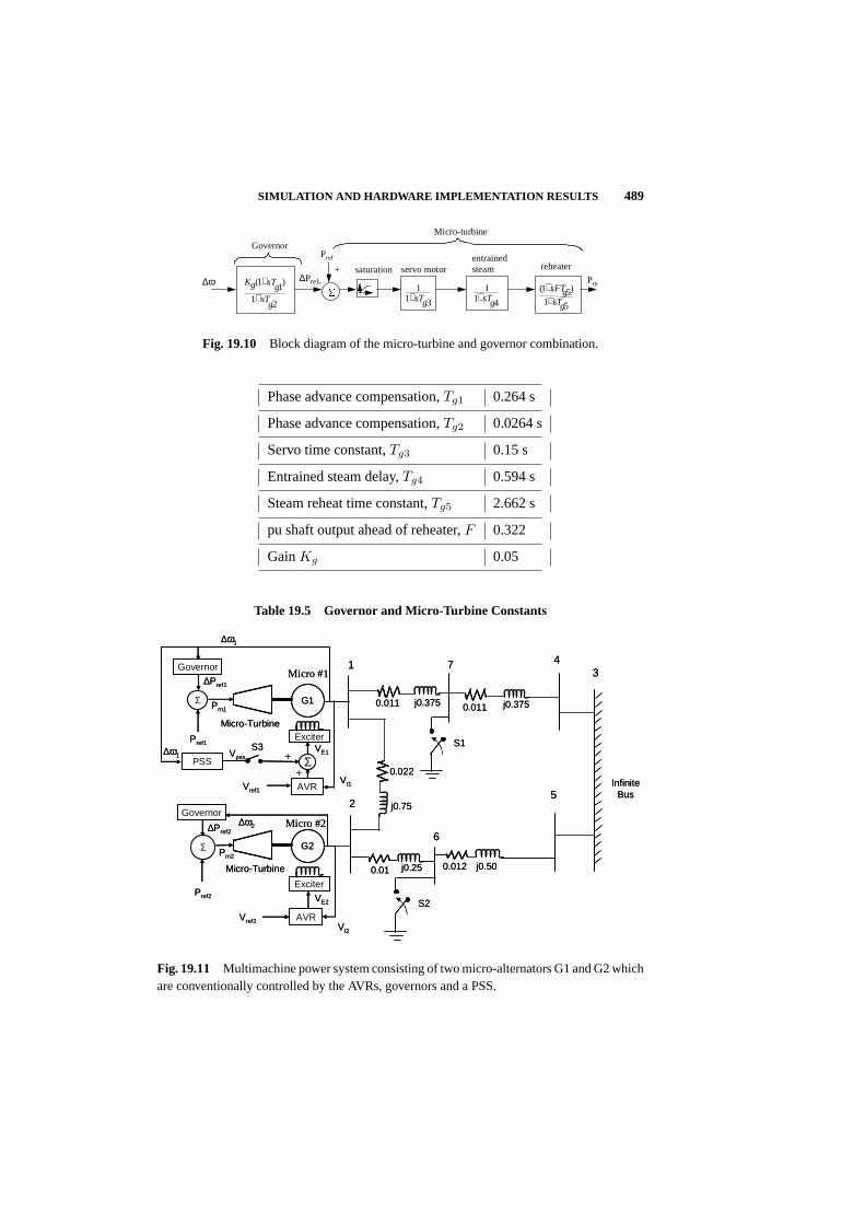
SIMULATION AND HARDWARE IMPLEMENTATION RESULTS 489
Kg sTgsTg
( )1 11 2
+
+1
1 3+sTg
11 4+sTg
( )1 51 5
++sFTgsTg
servo motorentrainedsteam reheatersaturation
GovernorPref
+- Pm ∆ω
Micro-turbine
∆Pref
Fig. 19.10 Block diagram of the micro-turbine and governor combination.
Phase advance compensation,Tg1 0.264 s
Phase advance compensation,Tg2 0.0264 s
Servo time constant,Tg3 0.15 s
Entrained steam delay,Tg4 0.594 s
Steam reheat time constant,Tg5 2.662 s
pu shaft output ahead of reheater,F 0.322
GainKg 0.05
Table 19.5 Governor and Micro-Turbine Constants
InfiniteBus
1
2
34
5
6
j0.375 j0.375
j0.50j0.25
S2
G1
Micro-TurbineExciter
Vref1
Pref1
G2
Micro-Turbine
Exciter
Vref2
Pref2
j0.75Governor
Σ
AVR
∆ω2
Vt2
Governor
AVRVt1
∆ω1
Σ
0.0120.01
0.0110.011
0.022PSS Σ+
+
∆ω1 VpssVE1
VE2
∆Pref1
∆Pref2
Micro #1
Micro #2
Pm1
Pm2
7
S1S3
InfiniteBus
1
2
34
5
6
j0.375 j0.375
j0.50j0.25
S2
G1
Micro-TurbineExciter
Vref1
Pref1
G2
Micro-Turbine
Exciter
Vref2
Pref2
j0.75Governor
Σ
AVR
∆ω2
Vt2
Governor
AVRVt1
∆ω1
Σ
0.0120.01
0.0110.011
0.022PSS Σ+
+
∆ω1 VpssVE1
VE2
∆Pref1
∆Pref2
Micro #1
Micro #2
Pm1
Pm2
7
S1S3
Fig. 19.11 Multimachine power system consisting of two micro-alternators G1 and G2 whichare conventionally controlled by the AVRs, governors and a PSS.
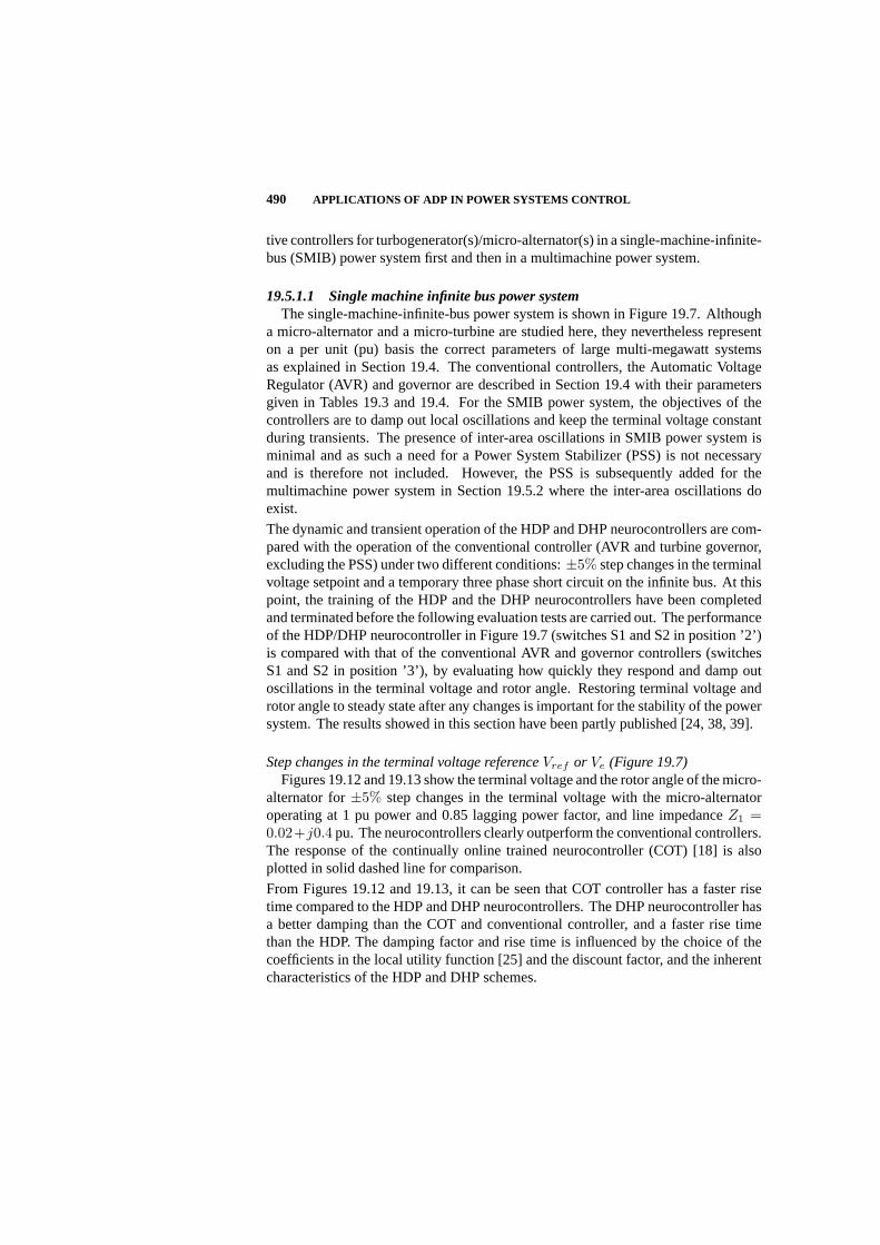
490 APPLICATIONS OF ADP IN POWER SYSTEMS CONTROL
tive controllers for turbogenerator(s)/micro-alternator(s) in a single-machine-infinite-bus (SMIB) power system first and then in a multimachine power system.
19.5.1.1 Single machine infinite bus power systemThe single-machine-infinite-bus power system is shown in Figure 19.7. Although
a micro-alternator and a micro-turbine are studied here, they nevertheless representon a per unit (pu) basis the correct parameters of large multi-megawatt systemsas explained in Section 19.4. The conventional controllers, the Automatic VoltageRegulator (AVR) and governor are described in Section 19.4 with their parametersgiven in Tables 19.3 and 19.4. For the SMIB power system, the objectives of thecontrollers are to damp out local oscillations and keep the terminal voltage constantduring transients. The presence of inter-area oscillations in SMIB power system isminimal and as such a need for a Power System Stabilizer (PSS) is not necessaryand is therefore not included. However, the PSS is subsequently added for themultimachine power system in Section 19.5.2 where the inter-area oscillations doexist.
The dynamic and transient operation of the HDP and DHP neurocontrollers are com-pared with the operation of the conventional controller (AVR and turbine governor,excluding the PSS) under two different conditions:±5% step changes in the terminalvoltage setpoint and a temporary three phase short circuit on the infinite bus. At thispoint, the training of the HDP and the DHP neurocontrollers have been completedand terminated before the following evaluation tests are carried out. The performanceof the HDP/DHP neurocontroller in Figure 19.7 (switches S1 and S2 in position ’2’)is compared with that of the conventional AVR and governor controllers (switchesS1 and S2 in position ’3’), by evaluating how quickly they respond and damp outoscillations in the terminal voltage and rotor angle. Restoring terminal voltage androtor angle to steady state after any changes is important for the stability of the powersystem. The results showed in this section have been partly published [24, 38, 39].
Step changes in the terminal voltage referenceVref or Ve (Figure 19.7)Figures 19.12 and 19.13 show the terminal voltage and the rotor angle of the micro-
alternator for±5% step changes in the terminal voltage with the micro-alternatoroperating at 1 pu power and 0.85 lagging power factor, and line impedanceZ1 =0.02+j0.4 pu. The neurocontrollers clearly outperform the conventional controllers.The response of the continually online trained neurocontroller (COT) [18] is alsoplotted in solid dashed line for comparison.
From Figures 19.12 and 19.13, it can be seen that COT controller has a faster risetime compared to the HDP and DHP neurocontrollers. The DHP neurocontroller hasa better damping than the COT and conventional controller, and a faster rise timethan the HDP. The damping factor and rise time is influenced by the choice of thecoefficients in the local utility function [25] and the discount factor, and the inherentcharacteristics of the HDP and DHP schemes.

SIMULATION AND HARDWARE IMPLEMENTATION RESULTS 491
0 5 10 15 20 25 301.05
1.1
1.15
1.2
1.25
1.3
Time in seconds
Ter
min
al v
olta
ge (
pu)
COTCONV
HDPDHP
Fig. 19.12 Terminal voltage of the micro-alternator for±5% step changes in the terminalvoltage reference (transmission line impedanceZ1).
0 5 10 15 20 25 3030
35
40
45
50
55
60
65
70
75
Time in seconds
Rot
or a
ngle
(de
gree
s)
COTCONV
HDPDHP
Fig. 19.13 Rotor angle of the micro-alternator for±5% step changes in the terminal voltagereference (transmission line impedanceZ1).
Short circuit test at new transmission line impedanceZ2
In power systems faults such as three phase short circuits occur from time totime, and because they prevent energy from the generator reaching the infinite bus,it means that most of the turbine shaft power goes into accelerating the generatorduring the fault. This represents a severe transient test for the controller performance.

492 APPLICATIONS OF ADP IN POWER SYSTEMS CONTROL
COT
CONV
HDPDHP
1 1.5 2 2.5 3 3.5 4 4.5
0.9
0.95
1
1.05
1.1
1.15
1.2
1.25
1.3
Time in seconds
Ter
min
al v
olta
ge in
pu
Fig. 19.14 Terminal voltage of the micro-alternator for a temporary 50 ms three phase shortcircuit (transmission line impedanceZ2).
0 1 2 3 4 5 6 745
50
55
60
65
70
75
80
Time in seconds
Loa
d an
gle
in d
egre
es
COTCONV
HDPDHP
Fig. 19.15 Rotor angle of the micro-alternator for a temporary 50 ms three phase short circuit(transmission line impedanceZ2).
Figures 19.14 and 19.15 show the response of all four controllers for the three phasetemporary short circuit for 50 ms with the new transmission line impedanceZ2. Here,it is obvious that the DHP controller clearly beats the other three controllers in termsof offering the greatest oscillation damping especially in the rotor angle. The DHPcontroller proves its robustness to changes in the system configurations.

SIMULATION AND HARDWARE IMPLEMENTATION RESULTS 493
19.5.1.2 Multimachine power systemThe multimachine power system is shown in Figure 19.11. The parameters of
the micro-alternators and conventional controllers are given in section 19.4 thischapter. Based on the results for the SMIB power system in section 19.5.1.1, theDHP controller has the best performance, hence, the DHP neurocontroller is the onlyone that is now implemented on the multimachine power system. The performance ofthe DHP neurocontroller is now compared with that of the conventional controllers,one of which is equipped with a power system stabilizer. Sections 19.5.1.2.1 and19.5.1.2.2 describe the multimachine power system with one DHP neurocontrollerand two DHP neurocontrollers respectively.
Multimachine power system with one DHP neurocontroller and one conventionalcontroller
The multimachine power system with one DHP neurocontroller and one conven-tional AVR and governor is shown in Figure 19.16. The design procedure of the DHPneurocontroller is similar to that of the SMIB power system described in sections19.2 and 19.3. The Model neural network training is carried out on a multimachinepower system as described in [39] and used with fixed weights in the design of theDHP neurocontroller in this section.
At different operating conditions and disturbances, the transient performance of theDHP neurocontroller is compared with that of the conventional controllers (AVR andgovernor), as well as with that of the AVR equipped with a PSS. For the operatingcondition (P1 = 0.20 pu,Q1 = -0.02 pu andP2 = 0.20 pu,Q2 = -0.02 pu), theconventional automatic voltage regulators, governors and the power system stabilizerare designed to give their best performance [7, 31].
Multimachine power system with two DHP neurocontrollersThe multimachine power system with DHP neurocontroller #1 and #2 controlling
micro-alternator #1 and #2 respectively is shown in Figure 19.17.
Three different controller combination studies are carried out, namely
• Casea - conventional controller on G1 and DHP neurocontroller on G2
• Caseb - conventional controller with a PSS on G1 and DHP neurocontrolleron G2
• Casec - DHP neurocontrollers on both G1 and G2.
At the operating condition (P1 = 0.20 pu,Q1 = -0.02 pu andP2 = 0.20 pu,Q2 = -0.02pu), a4% step increase occurs att = 1s in the desired terminal voltage (inVref1 inFigure 19.11 andVe1 in Figures 19.16 and 19.17) of micro-alternator #1. Figures19.18 and 19.19 show that the DHP neurocontrollers on the two micro-alternators(case c) ensure no overshoot on the terminal voltage unlike with casesa andb, andthat the DHP neurocontroller also provides superior speed deviation damping. Forthis same disturbance, Figure 19.20 shows the speed deviation of micro-alternator #2

494 APPLICATIONS OF ADP IN POWER SYSTEMS CONTROL
InfiniteBus
1
2
3
4
5
6
j0.375
j0.50j0.25
G1
Micro-TurbineExciter
Ve1
Pref1
G2
Micro-Turbine
Exciter
Vref2
Pref2
j0.75
Governor
Σ
AVR
∆ω2
Vt2
∆Vt1
Σ
0.0120.01
0.011
0.022
Σ+
+
∆ω1
VE1
VE2
∆Pref1
∆Pref2
DHPNeurocontroller
Ve1∆
Micro #2
Micro #1Pm1
Pm2
j0.3750.011
7
S1
Fig. 19.16 Multimachine power system with one DHP neurocontroller, and one conventionalAVR and governor.
InfiniteBus
1
2
3
4
5
6
j0.375 j0.375
j0.50j0.25
G1
Micro-Turbine TCR
Ve1
Pref1
G2
Micro-Turbine
TCR
Ve2
Pref2
j0.75
Σ
∆ω2
∆Vt2
∆Vt1
Σ
0.0120.01
0.0110.011
0.022
Σ+
+
∆ω1
VE1
VE2
∆Pref1
∆Pref2
DHPNeurocontroller #1
Ve1∆
Σ
DHPNeurocontroller #2
∆Ve2 +
+
Micro #1
Micro #2
7
S2
S1
Pm1
Pm2
Fig. 19.17 Multimachine power system with two DHP neurocontrollers.
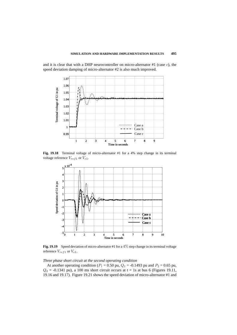
SIMULATION AND HARDWARE IMPLEMENTATION RESULTS 495
and it is clear that with a DHP neurocontroller on micro-alternator #1 (casec), thespeed deviation damping of micro-alternator #2 is also much improved.
1 2 3 4 5 6 7 8 9
0.99
1
1.01
1.02
1.03
1.04
1.05
1.06
1.07
Time in seconds
Ter
min
al v
olta
ge o
f G
1 in
pu
Case aCase b
Case c
1 2 3 4 5 6 7 8 9
0.99
1
1.01
1.02
1.03
1.04
1.05
1.06
1.07
Time in seconds
Ter
min
al v
olta
ge o
f G
1 in
pu
Case aCase b
Case c
Fig. 19.18 Terminal voltage of micro-alternator #1 for a 4% step change in its terminalvoltage referenceVref1 or Ve1.
0 1 2 3 4 5 6 7 8 9 10-5
-4
-3
-2
-1
0
1
2
3
4
5x 10⁻⁴
Time in seconds
Spee
d de
viat
ion
of G
1 in
pu
Case aCase b
Case c
0 1 2 3 4 5 6 7 8 9 10-5
-4
-3
-2
-1
0
1
2
3
4
5x 10⁻⁴
Time in seconds
Spee
d de
viat
ion
of G
1 in
pu
Case aCase b
Case c
Case aCase b
Case c
Fig. 19.19 Speed deviation of micro-alternator #1 for a4% step change in its terminal voltagereferenceVref1 or Ve1.
Three phase short circuit at the second operating conditionAt another operating condition (P1 = 0.50 pu,Q1 = -0.1493 pu andP2 = 0.65 pu,
Q2 = -0.1341 pu), a 100 ms short circuit occurs at t = 1s at bus 6 (Figures 19.11,19.16 and 19.17). Figure 19.21 shows the speed deviation of micro-alternator #1 and
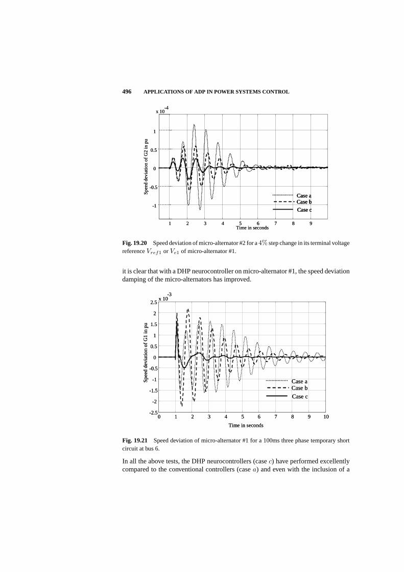
496 APPLICATIONS OF ADP IN POWER SYSTEMS CONTROL
1 2 3 4 5 6 7 8 9
-1
-0.5
0
0.5
1
x 10-4
Time in seconds
Spee
d de
viat
ion
of G
2 in
pu
Case aCase b
Case c
1 2 3 4 5 6 7 8 9
-1
-0.5
0
0.5
1
x 10-4
Time in seconds
Spee
d de
viat
ion
of G
2 in
pu
Case aCase b
Case c
Case aCase b
Case c
Fig. 19.20 Speed deviation of micro-alternator #2 for a4% step change in its terminal voltagereferenceVref1 or Ve1 of micro-alternator #1.
it is clear that with a DHP neurocontroller on micro-alternator #1, the speed deviationdamping of the micro-alternators has improved.
0 1 2 3 4 5 6 7 8 9 10-2.5
-2
-1.5
-1
-0.5
0
0.5
1
1.5
2
2.5x 10
-3
Time in seconds
Spe
ed d
evia
tion
of
G1
in p
u
Case aCase b
Case c
0 1 2 3 4 5 6 7 8 9 10-2.5
-2
-1.5
-1
-0.5
0
0.5
1
1.5
2
2.5x 10
-3
Time in seconds
Spe
ed d
evia
tion
of
G1
in p
u
Case aCase b
Case c
Case aCase b
Case c
Fig. 19.21 Speed deviation of micro-alternator #1 for a 100ms three phase temporary shortcircuit at bus 6.
In all the above tests, the DHP neurocontrollers (casec) have performed excellentlycompared to the conventional controllers (casea) and even with the inclusion of a

SIMULATION AND HARDWARE IMPLEMENTATION RESULTS 497
power system stabilizer (caseb) under different operating conditions. The resultsclearly prove the robustness of the DHP neurocontrollers which is as a result of thepowerful adaptive critic design algorithms. Many more tests were done to confirmthis The DHP neurocontrollers’ performances can be improved further by usingdifferent discount factors and local utility functions.
19.5.2 Hardware implementation
This section describes the laboratory practical implementation and testing of theDHP type ACD controllers. The purpose of these tests is to confirm via practicalmeasurements the potential of adaptive critic based neurocontrollers which have beendemonstrated during the simulation studies above, both for a single machine and amultimachine power system. However, the laboratory implementation on micro-machines is also intended to form a basis for possible future investigations into useof such neurocontrollers on large multi-megawatt sized power plants in a real-worldpower station.
19.5.2.1 Single machine infinite bus power system
A temporary 125 ms three phase short circuit at the first operating condition (P =0.2 pu,Q = 0 pu)
At the first operating condition, a temporary 125 ms duration three phase shortcircuit at bus B2 (Figure 19.7) is carried out att = 10 s. Figures 19.22 and 19.23 showthe terminal voltage and the load angle response for this test. DHP, PSS+CONV andCONV indicate for the response with the neurocontroller, the power system stabilizerplus the conventional controller, and the conventional controller respectively.
10 11 12 13 14 15 16 17 18 19 20
0.550.6
0.650.7
0.750.8
0.850.9
0.951
1.05
Time in seconds
Ter
min
al V
olta
ge in
pu
DHPPSS + CONVCONV
Fig. 19.22 Terminal voltage response for a temporary 125 ms three phase short circuit at busB2 (Figure 19.7) forP = 0.2 pu andQ = 0 pu.
The DHP neurocontroller again provides superior damping compared to the conven-tional controllers. In the terminal voltage response the DHP neurocontroller responds
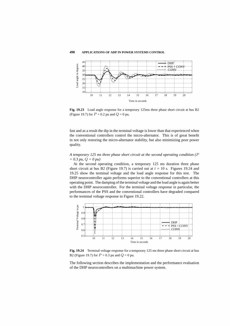
498 APPLICATIONS OF ADP IN POWER SYSTEMS CONTROL
10 11 12 13 14 15 16 17 18 19 2010
15
20
25
30
35
40
45
Time in seconds
Loa
d an
gle
in d
egre
es
DHPPSS + CONVCONV
Fig. 19.23 Load angle response for a temporary 125ms three phase short circuit at bus B2(Figure 19.7) forP = 0.2 pu andQ = 0 pu.
fast and as a result the dip in the terminal voltage is lower than that experienced whenthe conventional controllers control the micro-alternator. This is of great benefitin not only restoring the micro-alternator stability, but also minimizing poor powerquality.
A temporary 125 ms three phase short circuit at the second operating condition (P= 0.3 pu,Q = 0 pu)
At the second operating condition, a temporary 125 ms duration three phaseshort circuit at bus B2 (Figure 19.7) is carried out att = 10 s. Figures 19.24 and19.25 show the terminal voltage and the load angle response for this test. TheDHP neurocontroller again performs superior to the conventional controllers at thisoperating point. The damping of the terminal voltage and the load angle is again betterwith the DHP neurocontroller. For the terminal voltage response in particular, theperformances of the PSS and the conventional controllers have degraded comparedto the terminal voltage response in Figure 19.22.
10 11 12 13 14 15 16 17 18 19 200.5
0.6
0.7
0.8
0.9
1
Time in seconds
Ter
min
al V
olta
ge in
pu
DHPPSS + CONVCONV
Fig. 19.24 Terminal voltage response for a temporary 125 ms three phase short circuit at busB2 (Figure 19.7) forP = 0.3 pu andQ = 0 pu.
The following section describes the implementation and the performance evaluationof the DHP neurocontrollers on a multimachine power system.
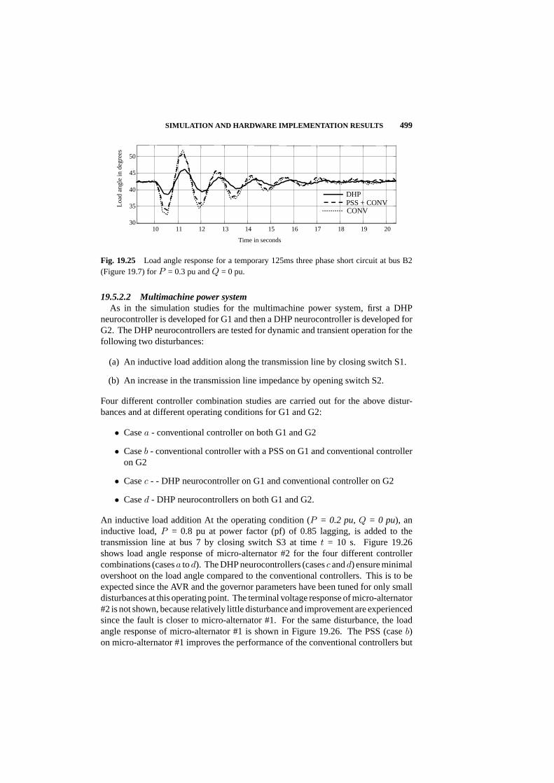
SIMULATION AND HARDWARE IMPLEMENTATION RESULTS 499
10 11 12 13 14 15 16 17 18 19 2030
35
40
45
50
Time in seconds
Loa
d an
gle
in d
egre
es
DHPPSS + CONVCONV
Fig. 19.25 Load angle response for a temporary 125ms three phase short circuit at bus B2(Figure 19.7) forP = 0.3 pu andQ = 0 pu.
19.5.2.2 Multimachine power systemAs in the simulation studies for the multimachine power system, first a DHP
neurocontroller is developed for G1 and then a DHP neurocontroller is developed forG2. The DHP neurocontrollers are tested for dynamic and transient operation for thefollowing two disturbances:
(a) An inductive load addition along the transmission line by closing switch S1.
(b) An increase in the transmission line impedance by opening switch S2.
Four different controller combination studies are carried out for the above distur-bances and at different operating conditions for G1 and G2:
• Casea - conventional controller on both G1 and G2
• Caseb - conventional controller with a PSS on G1 and conventional controlleron G2
• Casec - - DHP neurocontroller on G1 and conventional controller on G2
• Cased - DHP neurocontrollers on both G1 and G2.
An inductive load addition At the operating condition (P = 0.2 pu,Q = 0 pu), aninductive load,P = 0.8 pu at power factor (pf) of 0.85 lagging, is added to thetransmission line at bus 7 by closing switch S3 at timet = 10 s. Figure 19.26shows load angle response of micro-alternator #2 for the four different controllercombinations (casesa tod). The DHP neurocontrollers (casescandd) ensure minimalovershoot on the load angle compared to the conventional controllers. This is to beexpected since the AVR and the governor parameters have been tuned for only smalldisturbances at this operating point. The terminal voltage response of micro-alternator#2 is not shown, because relatively little disturbance and improvement are experiencedsince the fault is closer to micro-alternator #1. For the same disturbance, the loadangle response of micro-alternator #1 is shown in Figure 19.26. The PSS (caseb)on micro-alternator #1 improves the performance of the conventional controllers but
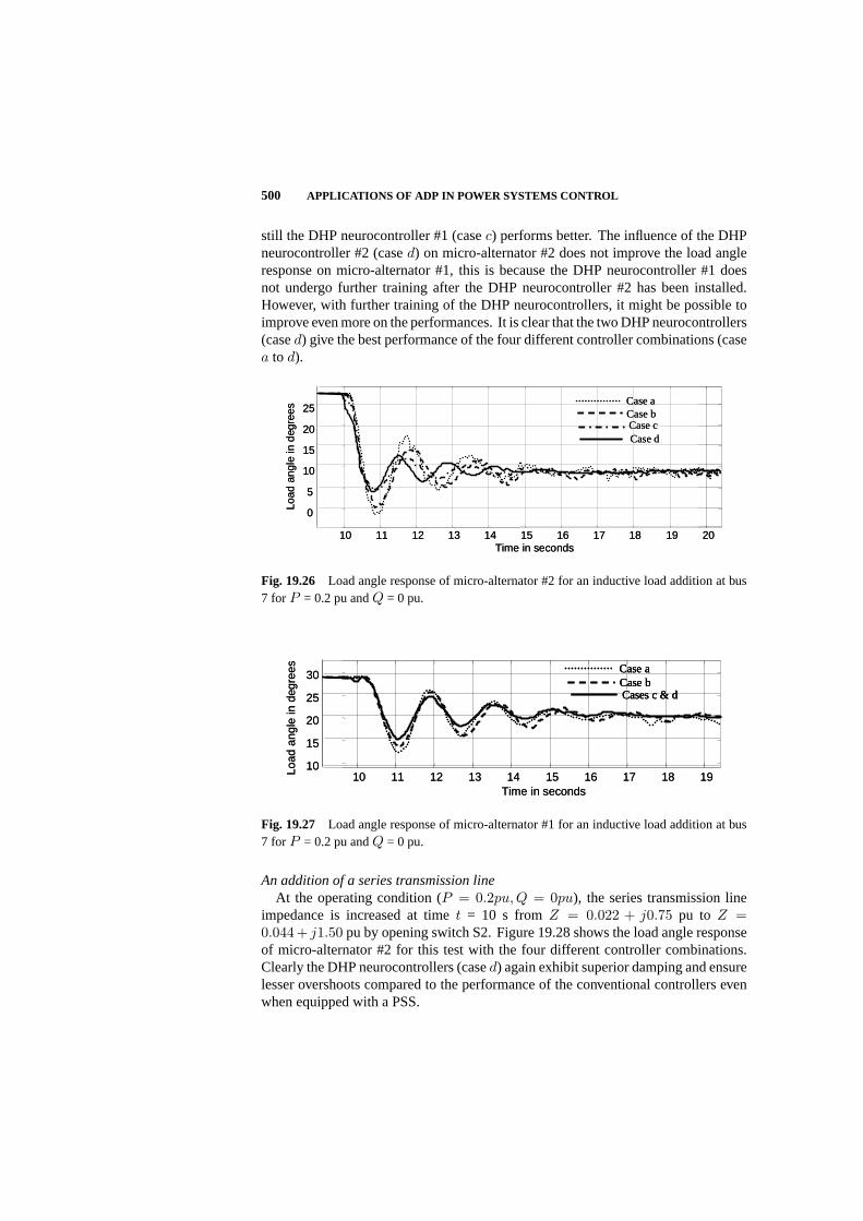
500 APPLICATIONS OF ADP IN POWER SYSTEMS CONTROL
still the DHP neurocontroller #1 (casec) performs better. The influence of the DHPneurocontroller #2 (cased) on micro-alternator #2 does not improve the load angleresponse on micro-alternator #1, this is because the DHP neurocontroller #1 doesnot undergo further training after the DHP neurocontroller #2 has been installed.However, with further training of the DHP neurocontrollers, it might be possible toimprove even more on the performances. It is clear that the two DHP neurocontrollers(cased) give the best performance of the four different controller combinations (casea to d).
10 11 12 13 14 15 16 17 18 19 20
0
5
10
15
20
25
Time in seconds
Load
ang
le in
deg
rees
Case cCase bCase a
Case d
10 11 12 13 14 15 16 17 18 19 20
0
5
10
15
20
25
Time in seconds
Load
ang
le in
deg
rees
Case cCase bCase a
Case dCase cCase bCase a
Case d
Fig. 19.26 Load angle response of micro-alternator #2 for an inductive load addition at bus7 for P = 0.2 pu andQ = 0 pu.
10 11 12 13 14 15 16 17 18 1910
15
20
25
30
Time in seconds
Load
ang
le in
deg
rees
Cases c & dCase bCase a
10 11 12 13 14 15 16 17 18 1910
15
20
25
30
Time in seconds
Load
ang
le in
deg
rees
Cases c & dCase bCase a
Cases c & dCase bCase a
Fig. 19.27 Load angle response of micro-alternator #1 for an inductive load addition at bus7 for P = 0.2 pu andQ = 0 pu.
An addition of a series transmission lineAt the operating condition (P = 0.2pu, Q = 0pu), the series transmission line
impedance is increased at timet = 10 s fromZ = 0.022 + j0.75 pu to Z =0.044 + j1.50 pu by opening switch S2. Figure 19.28 shows the load angle responseof micro-alternator #2 for this test with the four different controller combinations.Clearly the DHP neurocontrollers (cased) again exhibit superior damping and ensurelesser overshoots compared to the performance of the conventional controllers evenwhen equipped with a PSS.

SIMULATION AND HARDWARE IMPLEMENTATION RESULTS 501
10 11 12 13 14 15 16 17
20
22
24
26
28
Time in seconds
Load
ang
le in
deg
rees
Case cCase bCase a
Case d
10 11 12 13 14 15 16 17
20
22
24
26
28
Time in seconds
Load
ang
le in
deg
rees
Case cCase bCase a
Case dCase cCase bCase a
Case d
Fig. 19.28 Load angle response of micro-alternator #2 for series transmission line impedanceincrease by opening switch S2 forP = 0.2 pu andQ = 0 pu.
The load angle response of micro-alternator #1 for the same disturbance is shown inFigure 19.29. It is clear the DHP neurocontrollers exhibit the best damping of thecontrollers. Again, as in the case of the load addition disturbance result of Figure19.27, the addition of a DHP neurocontroller on micro-alternator #2 does not improvethe performance on micro-alternator #1. However, the performance could possiblybe improved if further training of the DHP neurocontrollers were to be carried out.
10.5 11 11.5 12 12.5 13 13.5 1410
15
20
25
30
Time in seconds
Load
ang
le in
deg
rees
10
Cases c & dCase bCase a
10.5 11 11.5 12 12.5 13 13.5 1410
15
20
25
30
Time in seconds
Load
ang
le in
deg
rees
10
Cases c & dCase bCase a
Fig. 19.29 Load angle response of micro-alternator #1 for series transmission line impedanceincrease by opening switch S2 forP = 0.2 pu andQ = 0 pu.
An inductive load addition at a different operating conditionAt the operating condition (P = 0.3pu,Q = 0pu), an inductive load,P = 0.8 pu at
power factor (pf) of 0.85, is added to the transmission line at bus 7 by closing switchS3 at timet = 10 s. Figure 19.30 shows the load angle response of micro-alternator #2for the four different controller combinations. The two DHP neurocontrollers (cased) ensure minimal overshoot and better damping of the load angle compared to theother controller combinations. This is to be expected since the conventional AVR andthe governor parameters have been tuned for only small disturbances at the operatingpoint (P = 0.2pu, Q = 0pu). For the same disturbance, the load angle response ofmicro-alternator #1 is shown in Figure 19.31. The PSS (caseb) on micro-alternator

502 APPLICATIONS OF ADP IN POWER SYSTEMS CONTROL
#1 improves the performance of the conventional controllers but still the DHP neu-rocontroller (casec) performs better. The influence of a DHP neurocontroller #2 onmicro-alternator #2 does not improve the load angle response on micro-alternator#1, because the DHP neurocontroller #1 does not undergo further training after DHPneurocontroller has been installed. However, with further training of the DHP neu-rocontrollers, it might be possible to improve more on the performances. It is clearthat the two DHP neurocontrollers give the best performance of the four differentcontroller combinations.
10 11 12 13 14 15 16 17 18 19 20
25
30
35
40
45
Time in seconds
Load
ang
le in
deg
rees
Case cCase bCase a
Case d
10 11 12 13 14 15 16 17 18 19 20
25
30
35
40
45
Time in seconds
Load
ang
le in
deg
rees
Case cCase bCase a
Case dCase cCase bCase a
Case d
Fig. 19.30 Load angle response of micro-alternator #2 for an inductive load addition at bus7 for P = 0.3 pu andQ = 0 pu.
10 15 20 2515
20
2530
35
4045
50
Time in seconds
Load
ang
le in
deg
rees
Cases c & dCase bCase a
10 15 20 2515
20
2530
35
4045
50
Time in seconds
Load
ang
le in
deg
rees
Cases c & dCase bCase a
Cases c & dCase bCase a
Fig. 19.31 Load angle response of micro-alternator #1 for an inductive load addition at bus7 for P = 0.3 pu andQ = 0 pu.
Additional tests, comparisons, and details on training and implementations are givenin [41, 42, 43].
19.6 SUMMARY
This chapter has presented the investigations on the design and implementation ofAdaptive Critic based neurocontrollers to replace the conventional automatic voltageregulators (AVRs) and governors on generators, in both a single-machine-infinite-bus
SUMMARY 503
and a multimachine power system. It has presented the concept for Adaptive CriticDesigns (ACDs) for the design of optimal controllers for practical power systemsand validated the concept on a laboratory prototype system.
For turbogenerators in a single-machine-infinite-bus power system, the results haveshown that it is possible to design and apply ACD based neurocontrollers based onHeuristic Dynamic Programming and Dual Heuristic Programming neurocontroller[24] that operate successfully. In addition the performances of ACD based neuro-controllers have been compared with the indirect adaptive neural controller based oncontinual online training, and also with the conventional automatic voltage regula-tor and governor [24]. From these comparisons it can be concluded that the DHPneurocontroller exhibits the best performance and robustness under many differentoperating conditions and system configurations.
The neurocontrolof turbogenerators in a SMIB power system has been extendedto DHP based neurocontrol of turbogenerators in a multi-machine power system.The performance and robustness of these DHP neurocontrollers have been comparedagainst the conventional AVRs and governors [25, 40] and in addition, with an AVRequipped with a conventional power system stabilizer [41]. Again, from these com-parisons it is concluded that the DHP neurocontroller exhibits the best performanceand robustness under different operating conditions and system configurations in themulti-machine power system.
The Adaptive Critic Designbased neurocontrollers have the great advantage thatonce trained, their weights/parameters remain fixed and therefore avoid the risk ofinstability associated with continual online training. The convergence guarantee ofthe Critic and Action neural networks during offline training was shown in [27, 42].In addition, the heavy computational load of online training only arises during theoffline training phase and therefore makes the online real time implementation costof the neurocontrollers cheaper. The processing hardware cost is a small fraction ofthe cost of turbogenerators and therefore this is not a big issue.
TheAdaptive Critic Designbased nonlinear neurocontrollers designed in this chapterare all based on approximate models obtained by neuroidentifiers, but neverthelessexhibit superior performance in comparison to the conventional linear controllerswhich use more extensive linearized models. This benefit of a neuroidentifier agreeswith the conclusions on the comparison of using approximate and exact models inadaptive critic designs which was explicitly shown in [28].
All these features are desirable and important for industrial applications which requirea neurocontroller technology that is nonlinear, robust and stable.
Acknowledgments
The authors acknowledge the University of Natal, Durban, South Africa for allowing the usageof the micro-machines laboratory. The financial support from the National Science Foundation,USA and National Research Foundation, South Africa, are also gratefully acknowledged.

Bibliography
1. B. Adkins, R.G. Harley,The general theory of alternating current machines,Chapman and Hall, London, ISBN 0-412-15560-5, 1975.
2. Q.H. Wu , B.W. Hogg, “Laboratory Evaluation of Adaptive Controllers forSynchronous Generators,”Automatica,vol. 27, no. 5, pp. 845 - 852, 1991.
3. Q.H. Wu , B.W. Hogg, “Adaptive Controller for a Turbogenerator System,”IEEProceedings,vol. 135, Pt D, no. 1, pp. 35-42, 1988.
4. O.P. Malik, C.X. Mao, K. Prakash, G. Hope, G. Hancock, “Tests with a Mi-crocomputer based Adaptive Synchronous Machine Stabilizer on a 400 MWThermal Unit,”IEEE Trans. on Electronic Computation,vol. 8, no. 1, pp. 6 - 12,1992.
5. D. Flynn, B.W. Hogg, E. Swidenbank, K.J. Zachariah, “Expert Control of a Self-Tuning Automatic Voltage Regulator,”Control Engineering Practice,vol. 3,no. 11, pp. 1571 - 1579, 1995.
6. D.J.G. Morrell, B.W. Hogg, “Identification and Validation of TurbogeneratorsModels,”Automatica,vol. 26, no. 1, pp 135 -156, 1990.
7. P. Kundur, M. Klein, G.J. Rogers, M.S. Zywno, “Application of Power SystemStabilizers for Enhancement of Overall System Stability,”IEEE Trans. on PowerSystems,vol. 4, no. 2, pp. 614 - 626, May 1989.
8. F.P. deMello, C. Concordia, “Concepts of Synchronous Machine Stability asAffected by Excitation Control,”IEEE Trans. on Power Apparatus and Systems,vol. PAS-87, pp. 1426-1434, 1968.
9. M.R. Khaldi, A.K. Sarkar, K.Y. Lee, Y.M. Park, “The Modal Performance Mea-sure of Parameter Optimization of Power System Stabilizers,”IEEE Trans. onEnergy Conversion,vol. 8, no. 4, pp. 660 - 666, December 1993.
10. P.M. Anderson, A.A. AndersonFouad,Power System Control and Stability,ISBN0-7803-1029-2, IEEE Press, New York, 1994.
11. Y. Kitauchi, H. Taniguchi, “Experimental Verification of Fuzzy Excitation Con-trol System for Multi-Machine Power System,”IEEE Trans. on Energy Conver-sion,vol. 12, no. 1, pp. 94 - 99, March 1997.
504
BIBLIOGRAPHY 505
12. J.W. Chapman, M.D. Ilic, C.A. King, L. Eng, H. Kaufman, “Stabilizing a Mul-timachine Power System via Decentralized Feedback Linearizing ExcitationControl,” IEEE Trans. on Powers System,vol. 8, no. 3, pp. 830-839, August1993.
13. Y. Wang, D.J. Hill, L. Gao, R.H. Middleton, “Transient Stability Enhancementand Voltage Regulation of Power System,”IEEE Trans. on Power System,vol. 8,pp. 620-627, 1993.
14. Z. Qiu, J.F. QiuDorsey, J. QiuDorseyBond, J.D. McCalley, “Application ofRobust Control to Sustained Oscillations in Power Systems,”IEEE Trans. onCircuits System I: Fundamental Theory and Applications,vol. 39, no. 6, pp. 470-476, June 1992.
15. K.S. Narendra, K. Parthasarathy, “Identification and Control of Dynamical Sys-tems using Neural Networks,”IEEE Trans. on Neural Networks,Vol.1, no. 1,pp. 4-27, March 1990.
16. K.J. Hunt, D. Sbarbaro, R. Zbikowski, R.J. Gawthrop, “Neural Networks forControl Systems - a Survey,”Automatica,vol. 28, no. 6, pp. 1083 - 1112, 1992.
17. G.K. Venayagamoorthy, R.G. Harley, “ A Continually Online Trained ArtificialNeural Network Identifier for a Turbogenerator,”Proceedings of IEEE Inter-national Electrical Machine and Drives Conference (IEMDC),Seattle, USA,pp. 404 - 406, May 1999.
18. G.K. Venayagamoorthy, R.G. Harley, “A Continually Online Trained Neuro-controller for Excitation and Turbine Control of a Turbogenerator,”IEEE Trans.on Energy Conversion,vol. 16, No.3, pp. 261-269, September 2001.
19. P. Parks, “Liapunov Redesign of Model Reference Adaptive Control Systems“IEEE Trans. on Automatic Control,vol. 11, pp. 362-367, 1966.
20. P. Osburn, Whitaker H, Kezer A, “New Developments in the Design of ModelReference Adaptive Control Systems,”Proceedings of the IAS 29th AnnualMeeting,New York, 1961.
21. R.M. Sanner, J.E. Sanner Slotine, “Gaussian Networks for Direct Adaptive Con-trol,” IEEE Trans. on Neural Networks,vol. 3, no. 6, pp. 837-863, November1992.
22. M.I. Jordan, D.E. Rumelhart, “Forward Models: Supervised Learning with aDistal Teacher,”Cognitive Science,vol. 16, pp. 307-354, 1992.
23. A.U. Levin, K.S. Narenda, “Control of Nonlinear Dynamical Systems usingNeural Networks: Controllability and Stabilization,”IEEE Trans. on NeuralNetworks,vol. 4, no. 2, pp. 192-206, March 1993.
24. G.K. Venayagamoorthy, R.G. Harley, D.C. Wunsch,“Comparison of HeuristicDynamic Programming and Dual Heuristic Programming Adaptive Critics for
506 BIBLIOGRAPHY
Neurocontrol of a Turbogenerator,”IEEE Transactions on Neural Networks,vol. 13, Issue 3, pp. 764 -773, May 2002.
25. G.K. Venayagamoorthy, R.G. Harley, D.C. Wunsch, “Dual Heuristic Program-ming Excitation Neurocontrol for Generators in a Multimachine Power System,”IEEE Transactions on Industry Applications,Vol. 39, Issue: 2, pp. 382-384,March/April 2003.
26. G.K. Venayagamoorthy, R.G. Harley, D.C. Wunsch, “Implementation of Adap-tive Critic Based Neurocontrollers for Turbogenerators for Turbogenerators in aMultimachine Power System,”IEEE Transactions on Neural Networks,vol. 14,no. 5, pp. 1047-1064, September 2003.
27. D. Prokhorov, L.A. Feldkamp, “Analyzing for Lyapunov Stability with AdaptiveCritics,” Proceedings of the International Conference on Systems, Man andCybernetics,vol. 2, pp. 1658-1161, 1998.
28. T.T. Shannon, G.G. Lendaris, “Qualitative Models for Adaptive Critic Neuro-control,”Proceedings of the International Joint Conference on Neural Networks,IJCNN 1999, Washington DC, USA, vol. 1, pp. 455-460, 1999.
29. Z. LendarisHuang, S.N. Balakrishnan, “Robust Adaptive Critic Based Neurocon-trollers for Systems with Input Uncertainties,”Proceedings of the InternationalJoint Conference on Neural Networks, (IJCNN 2000),Como, Italy, vol. 3, pp. 67-72, 24 - 27 July, 2000.
30. D.J. Limebeer, R.G. Harley, S.M. Schuck, “Subsychronous Resonance of theKoeberg Turbogenerators and of a Laboratory Micro-Alternator System,”Trans.of the SA Institute of Electrical Engineers,pp. 278-297, November 1979.
31. W.K. Ho, C.C. Hang, and L.S. Cao, “Tuning of PID Controllers based on Gain andPhase Margin Specifications,”Proceedings of the 12th Triennial World Congresson Automatic Control,pp. 199 -202, 1993.
32. P.J. Werbos, “Approximate Dynamic Programming for Real Time Control andNeural Modelling,” in White DA and Sofge DA (Eds.),Handbook of IntelligentControl, ISBN 0-442-30857-4, Van Nostrand Reinhold, New York, pp. 493 -525, 1992.
33. Anthony R. Cassandra, Leslie P. Kaelbling, and Michael L. Littman, “Acting Op-timally in Partially Observable Stochastic Domains,”Proceedings of the TwelfthNational Conference on Artificial Intelligence (AAAI-94),vol. 2, pp. 1023-1028,1994.
34. C.J. Watkins, P. Dayan, “Q-Learning,”Machine Learning,vol. 8, pp. 279 - 292,1992.
35. D.V. Prokhorov, “Adaptive Critic Designs and their Applications,”Ph.D. Thesis,Texas Tech University,USA, October 1997.

BIBLIOGRAPHY 507
36. D.V. Prokhorov, D.C. Wunsch, “Adaptive Critic Designs“IEEE Trans. on NeuralNetworks,vol. 8, no. 5, pp. 997 - 1007, September 1997.
37. G.K. Venayagamoorthy, R.G. Harley, D.C. Wunsch, “Adaptive Neural NetworkIdentifiers for Effective Control of Turbogenerators in a Multimachine PowerSystem,”Proceedings of IEEE Power Engineering Society Winter Meeting 2001,Columbus, Ohio, USA, pp. 1293 - 1298, 28 January - 1 February, 2001.
38. G.K. Venayagamoorthy, D.C. Wunsch, R.G. Harley, “Neurocontrol of Turbo-generators with Adaptive Critic Designs,”Proceedings of IEEE Africon,CapeTown, South Africa, pp. 489 - 494, 28 September - 2 October 1999.
39. G.K. Venayagamoorthy, R.G. Harley, D.C. Wunsch, “Comparison of a HeuristicDynamic Programming and a Dual Heuristic Programming Based Adaptive Crit-ics Neurocontroller for a Turbogenerator,”International Joint Neural NetworksConference (IJCNN 2000),Como, Italy, vol. 3, pp. 233 - 238, 24 - 27 July, 2000.
40. G.K. Venayagamoorthy, R.G. Harley, D.C. Wunsch, “Excitation and TurbineNeurocontrol with Derivative Adaptive Critics of Multiple Generators on thePower Grid,” IEEE-INNS International Joint Conference on Neural Networks,Washington DC, USA, pp. 984-989, 15-19 July, 2001.
41. G.K. Venayagamoorthy, R.G. Harley, D.C. Wunsch, “A Nonlinear Voltage Con-troller with Derivative Adaptive Critics for Multimachine Power Systems,”IEEEPower Industry Computer Applications Conference (PICA),Sydney, Australia,pp. 324-329, 20 - 24 May, 2001.
42. D.V. Prokhorov, D.C. Wunsch, “Convergence of Critic-Based Training,”Pro-ceedings of the IEEE International Conference on Systems, Man, and Cybernet-ics,vol. 4, pp. 3057 - 3060, 1997.

20 Robust Reinforcement Learningfor Heating, Ventilation, and AirConditioning Control ofBuildings
CHARLES W. ANDERSON, DOUGLAS HITTLE, MATT KRETCH-MAR, and PETER YOUNG
Colorado State University
Editor’s Summary: This chapter is a case study, implementing the techniquepresented in Chapter 13. A detailed problem formulation is presented for a heatingand cooling system and a step-by-step solution is discussed. A combined PI andreinforcement learning controller is designed within a robust control framework anddetailed simulation results are presented and an internet link is provided to a websitewhere information on experiments is provided.
20.1 INTRODUCTION
Typical methods for designing fixed feedback controllers result in sub-optimal controlperformance. In many situations, the degree of uncertainty in the model of the systembeing controlled limits the utility of optimal control design. Controllers can bemanually tuned in the field, but it is very difficult to determine manual adjustments thatresult in overall improvement. Building energy systems are particularly troublesomesince the process gain is highly variable, depending non-linearly on the load oncomponents such as heating and cooling coils and on inlet conditions such as airtemperature and air volume flow rate.
With the development and implementation of high speed digital control hardware,researchers in the HVAC industry have begun to explore self-tuning control systemsfor heating and air-conditioning processes. Heating and air-conditioning processespose especially difficult control tuning issues because the gain of the system canvary with load and vary seasonally. For example, Figure 20.1 shows the percent
508

INTRODUCTION 509
PercentCapacity
Percent Flow
0
100
0 100
Fig. 20.1 Percent of capacity of a heating coil versus hot water flow rate through the coil.
of capacity of a heating coil versus hot water flow rate through the coil (data frommanufacturer’s software). Notice how much more rapidly capacity changes withchanges in flow at low flow rates than at high flow. Even if a compensating non-linear valve is used to control the coil, the performance of the combination may havevariable gain depending on how much pressure drop occurs in the valve compared tothe coil. The heating coil/valve system gain also changes with air flow rate and inletwater and air temperatures. In many HVAC subsystems individual loop gains changesignificantly with the state of the overall system.
Some of these issues have been addressed by Nesler and Stoecker [27] and Bekker,Meckel and Hittle [8]. These authors proposed various manual tuning strategies forheating and air-conditioning processes, which consequently require skilled humanoperators.
Self-tuning techniques have also been proposed. Brandt [9] summarizes severalapproaches to adaptive control. He makes the important point that so-called "jacket"software often needs to be implemented along with the adaptive control schemes toavoid trying to tune when the system is uncontrollable (for example, when the heatingcoil is off) or when variations are so slow as to make adaptation inappropriate. Pinellaet al. [30] and Dexter and Haves [15] describe some implementations of self-tuningprocedures. More recently, Seem [32] proposed a new pattern recognition adaptivecontroller (PRAC) that adjusts the proportional and integral gain to stabilize unstablePI controllers.
Expert systems are also being considered. For example Haberl et al. [20] discuss ex-pert systems used to diagnose operating malfunctions in heating and air-conditioningsystems. Norford et al. [28] discuss the implementation of a similar expert system tohelp building operators in determining proper operating strategies.

510 ROBUST REINFORCEMENT LEARNING FOR HVAC
Most recently, researchers have begun to consider using neural networks to controlthe highly non-linear and time varying HVAC processes. Ferrano and Wong [19], forexample, use neural networks as a weather predicting strategy in applications involv-ing thermal storage. Other examples include Seem and Braun’s [33] use of neuralnetworks to predict electrical demand and Miller and Seem’s [25] prediction of timerequired to return a room to a desired temperature. Hepworth and Dexter [21] used aneural network of radial basis functions in parallel with a proportional controller onan HVAC system. They showed, by simulation and experiment, that their controllercan compensate for plant non-linearities and adapt to plant degradation over time.Curtiss et al. [13, 12] used a neural network controller to gradually take over from aPID controller. Ahmed et al. [1] applied general regression neural networks to HVACprocess control. Shavit, in Curtiss et al. [14] used a neural network to augment theoutput of a PI controller. The network attempts to modify the output of a PI controllerto provide first order response of the process while minimizing the actuator motion.The network is trained off-line, using simulation models of the various systems towhich it is to be applied. This scheme has been field tested with better than expectedresults.
Concepts developed by Shavit and Seems [34] have been field-tested, indicatingthat they are more fully developed than others. Seem’s PRAC controller uses thetemporal pattern of the controlled variable to adjust the proportional and integral gainconstants of a PI controller to stabilize and improve the performance of the system.Note that while this scheme is adaptive, the plant is still controlled by a traditionalsingle-input—single-output PI controller.
Shavit uses a fixed (trained off line) neural network in parallel with a PI controller asa replacement for a traditional PI controller. The neural network plays the role of anon-linear controller that is well suited to non-linear HVAC systems.
In summary, both Seem and Shavit use single-input—single-output (SISO) feedbackcontrollers, which is typical of current practice in the HVAC industry. The enormouspotential of powerful techniques for MIMO control has not been explored in HVACsystems. Seem’s scheme is linear but adaptive while Shavit’s is nonlinear but fixed.
The neural network control schemes enumerated above have all used supervisedlearning, generally with back-propagation as the method for weight adjustment. Thepotential of reinforcement (unsupervised) learning is largely unexplored for HVACcontrol problems.
An alternate approach to designing a controller that attempts to learn about theunknown dynamics of a system is to design one that is insensitive to such modeluncertainties. This is the subject of robust control. This area has seen a great dealof research activity in recent years, with powerful new tools for system analysis andcontroller design emerging.
Early researchers in this area, including Doyle [16] and Safonov [31], developedstability analysis tools for multivariable linear time invariant (LTI) systems subject tostructured dynamic LTI uncertainties. This work was extended toH∞ performanceanalysis and controller synthesis in Doyle [17]. Subsequent work in this area has ledto machinery for parametric uncertainty in Young [40] and Barmish and Kang [6],

INTRODUCTION 511
and nonlinear or time-varying uncertainty in Shamma [35] and Megretsky [24]. Toolsare now available that use alternative norms for the performance measure, such asH2 in Paganini [29],L1 in Khammash and Pearson [23], and extensions to arbitraryLp-induced norms for the LTI case in Bamieh and Dahleh [5] and the nonlinear/time-varying case in Young and Dahleh [41]. More recently, some tools have started toemerge for performance measures other than norms, and in particular fixed inputs areconsidered in Elia et al. [18].
In tandem with this theoretical work, researchers have developed advanced compu-tational software, such as theµ-Tools Matlab toolbox (Balas et al. [4]), which hasfacilitated the use of this work by practicing engineers in industry. Robust designshave been successfully applied to many interesting practical problems (Balas andYoung [3]; Buschek and Calise [10]), though their utility for HVAC systems has yetto be considered.
A natural question that arises from this is to consider whether reinforcement learn-ing and robust control can be usefully combined. Indeed, in his summary paperWerbos [39] remarks, “Most practical applications probably involve a mix of knownand unknown dynamics, so that the ultimate optimum is to combine these two ap-proaches.” Some researchers have started to consider this possibility. These ideashave been exploited to address the well-known stability problems of classical adap-tive control schemes. Although this innovation is fairly recent, there has already beenconsiderable success, and the ideas are now mainstream enough to find texts on thesubject, such as Ioannou and Sun [22]. However, for learning controllers, only a verylimited amount of work has been carried out in this direction. Suykens et al. [37] usea neural net to identify a plant model in the canonical linear fractional transformation(LFT) form with associated uncertainty description, so that this identified model setcan then be used for a robust design. Bass and Lee [7] use a neural net to learnthe dynamic inversion of a nonlinear plant, and implement feedback linearization,so that a robust design can then be carried out for the linearized plant. It shouldbe noted however that efforts in this regard are still in their infancy, and none ofthe approaches developed so far really exploits the power of both approaches. Forinstance, in both of the above examples one can only ever get the performance thatthe robust controller can deliver, and the neural net is essentially helping with theidentification/linearization. However, one would like to exploit the power of a neuralnet controller to precisely tune the controller, so that the final delivered performanceexceeds that of a robust controller based only on a-priori information.
In this chapter, a reinforcement-learning (RL) agent is added in parallel to an existingfeedback controller and trained to minimize the sum of the squared error of thecontrol variable over time. First, results are shown of RL learning performance whenapplied to a non-linear simulation of a heating coil. Then, the system consisting ofthe heating coil model, a proportional-integral (PI) feedback controller, and RL agentare placed in the robust control framework described in Chapter 13. The heating coilmodel is linearized and integral-quadratic constraints (IQC) are used to characterizethe non-linear and time-varying parts of the RL agent. This results in a synthesis
512 ROBUST REINFORCEMENT LEARNING FOR HVAC
of feedback control and reinforcement learning with guaranteed static and dynamicstability, even while learning.
20.2 HEATING COIL MODEL AND PI CONTROL
Underwood and Crawford [38] developed a model of an existing heating coil byfitting a set of second-order, non-linear equations to measurements of air and watertemperatures and flow rates obtained from the heating coil. A diagram of the modelwith a PI controller is shown in Figure 20.2. The state of the modeled system isdefined by the air and water input and output temperatures,Tai, Tao, Twi, Two,and the flow rates of air and water,fa, andfw. The control signal,c, affects thewater flow rate. Its value ranges from 670 for the maximally-open position to 1400for the maximally-closed position. By changing the valve setting, the flow rate ofthe water in the heating coil can be increased or decreased. The valve setting, aninput to the plant, is the output from the controllers. The flow rate of water,fw, isdirectly affected by the valve setting. In turn, this affects the temperature of the waterleaving the coil,Two, and ultimately the temperature of the air leaving the coil,Tao,because the flow rate of the water determines how much thermodynamic energy canbe delivered from the boiler to the heating coil in the duct.Tao is the state variablethat is to be controlled. Control performance is determined by how closely the outputair temperature tracks the reference signal, which, in the HVAC case, is the desiredthermostat setting or the set point.
The model is given by the following equations with constants determined by a least-square fit to data from an actual heating coil:
fw(t) = 0.008 + 0.00703(− 41.29 + 0.30932c(t− 1)
−3.2681× 10⁻⁴c(t− 1)2 + 9.56× 10⁻⁸c(t− 1)3), (20.1)
Two(t) = Two(t− 1) + 0.64908fw(t− 1)(Twi(t− 1) (20.2)
−Two(t− 1))
+(0.02319 + 0.10357fw(t− 1) +
0.02806fa(t− 1))(
Tai(t− 1)− (Twi(t− 1) + Two(t− 1))2
),
Tao(t) = Tao(t− 1) + 0.19739fa(t− 1)(Tai(t− 1)
−Tao(t− 1))− (
0.03184 + 0.15440fw(t− 1)
+0.04468fa(t− 1))(
Tai(t− 1)− (Twi(t− 1) + Two(t− 1))2
)
+0.20569(Tai(t)− Tai(t− 1)
). (20.3)
For the experiments reported here, the variablesTai, Twi, andfa were modified byrandom walks to model the disturbances and changing conditions that would occurin actual heating and air conditioning systems. The bounds on the random walks are4 ≤ Tai ≤ 10oC, 73 ≤ Twi ≤ 81oC, and0.7 ≤ fa ≤ 0.9 kg/s.

COMBINED PI AND REINFORCEMENT LEARNING CONTROL 513
Temp Water In
Temp H20 Out
Mass Flow
Rate Water
Temp Air In
Mass Flow Air
Duct
Temp Air Out
PI ControllerTemp Set Point
Tai
fa
Twi
fw T
wo
Tao
c
Fig. 20.2 The simulated heating coil under control of a PI feedback controller.
A PI controller was tuned to control the simulated heating coil. The best proportionaland integral gains were determined by measuring the sum of the absolute value ofthe difference between the set point and the actual exiting air temperature under avariety of disturbances. The PI control law is
c′(t) = kpe(t) + ki
∫e(t) dt, (20.4)
wheree(t) is the difference between the set point and the actual output air temperatureat timet, kp is the proportional gain, andki is the integral gain.c′(t) is a normalizedcontrol value that ranges from 0 to 1 to specify flows rates from the minimum tothe maximum allowed values. The best control law constants were determined tobekp = 0.185 andki = 0.178. This normalized control signal is converted to thecontrol signal for the model by
c(t) = 1400− 730c′(t). (20.5)
20.3 COMBINED PI AND REINFORCEMENT LEARNING CONTROL
A reinforcement learning agent trained using the Q-learning algorithm [42, 36] wascombined with a PI controller as shown in Figure 20.3. Inputs to the reinforcement-learning agent wereTai, Tao, Twi, Two, fa, fw, and the set point, all at timet. Theoutput of the reinforcement learning agent is directly added to the output of the PIcontroller. The allowed output actions of the reinforcement learning agent was theset of discrete actionsA = −100,−50,−20,−10, 0, 10, 20, 50, 100. The selectedaction is added to the PI control signal. TheQ function is implemented using aquantized, or table look-up, method. Each of the seven input variables is divided

514 ROBUST REINFORCEMENT LEARNING FOR HVAC
Temp Water In
Temp H20 Out
Mass Flow Rate Water
Temp Air In
Mass Flow Air
Duct
Temp Air Out
ReinforcementLearning Agent
PI Controller
Temp Set Point
Tai
fa
Twi
fw
Two
Tao
c
Other Variables:
T
T T
f f
ai
wi wo
a w
Fig. 20.3 The heating coil controlled by the sum of a PI controller and the action taken bythe reinforcement learning agent.
into six intervals, which quantize the 7-dimensional input space into67 hypercubes.UniqueQ values for the nine possible actions are stored in each hypercube.
ReinforcementR at time stept is determined by the squared error between thecontrolled variable and its set point plus a term proportional to the square of theaction change from one time step to the next:
R(t) = (Tao(t)∗ − Tao(t))2 + β(at − at−1)2, (20.6)
whereT ∗ao is the set point. The action change term is introduced to reduce thefluctuation in the control signal to minimize the stress on the control mechanism.The values ofat in this equation are indices of the setA, rather than actual outputvalues.
The reinforcement-learning agent is trained for 1,000 repetitions, calledtrials, of a500 time-step interaction between the simulated heating coil and the combination ofthe reinforcement learning agent and the PI controller, hereafter referred to as theRL/PI controller. The performance of the RL/PI controller was compared with theperformance of just the PI controller. Figure 20.4 shows the set point and actualtemperatures and the PI control signal over these 500 steps. The RMS error betweenthe set point and actual output air temperature over these 500 steps for the PI controlleracting alone is 0.93.
The training algorithm for the reinforcement learning agent depends on the parametersαt, λ, γ, andβ. After trying a small number of values,γ andβ were fixed toγ = 0.95andβ = 0.1. A number of combinations of values forα andλ were tested, whereαis held constant during a training run rather than setting it to values that decrease withtime as required for the convergence proofs. Figure 20.5 shows how performance

COMBINED PI AND REINFORCEMENT LEARNING CONTROL 515
0 50 100 150 200 250 300 350 400 450 50030
40
50
Tai
0 50 100 150 200 250 300 350 400 450 500500
1000
1500
c
(control signal)
Fig. 20.4 Performance of PI controller. The top graph shows the set point and the actualoutput air temperature over time. Over this sequence, the RMS error is 0.93. The bottomgraph shows the PI output control signal.
depends on these parameter values. Performance was measured by the average RMSerror over the final 30 trials and also by the average RMS error over all 1,000 trials.The first measure is of final performance and the second is an indication of the speedwith which the error was reduced. The best parameter values wereα = 0.1 andλ = 0.995. These values were used to obtain the following results.
The reduction in RMS error while training the reinforcement-learning agent is shownin Figure 20.6. After approximately 80 training trials, the average RMS error betweenthe set point and actual temperature was reduced below the level achieved by the PIcontroller alone. With further training the reinforcement learning agent convergeson a deterministic policy that consistently achieves an RMS error of 0.85, about an8.5% reduction in error from that achieved by the PI controller alone.
The resulting behavior of the controlled air temperature is shown in the first graph ofFigure 20.7. The second graph shows the output of the reinforcement-learning agent.It has learned to be silent (an output of 0) for most time steps. It produces largeoutputs at set point changes and at several other time steps. The combined output ofthe RL/PI controller is shown in the third graph. The reinforcement-learning agentlearns to augment the PI controller’s output during the initial steps and at most of theset point changes. From time step 340 through about 480 the reinforcement-learningagent injects negative and positive values into the control signal. This pattern ofoutputs to which the controller converged on in most of the successful training runsof the reinforcement-learning agent. This behavior is due to the particular trajectoriesfollowed by the disturbance variables. The last three graphs of Figure 20.7 showsthe disturbance trajectories forTai, Twi, andfa. At step 340 the value offa exceedsits previous values and the reinforcement learning agent compensates by injecting apattern of negative and positive changes to the controller’s output. Additional detailsof these experiments are described by Anderson, et al. [2].

516 ROBUST REINFORCEMENT LEARNING FOR HVAC
α = 0.001
α = 0.01
α = 0.1
α = 0.5
0.94 0.95 0.96 0.97 0.98 0.99 10.8
1
1.2
1.4
1.6
λ
α = 0.001
α = 0.01
α = 0.1
α = 0.5
0.94 0.95 0.96 0.97 0.98 0.99 10.8
1
1.2
1.4
RMS Error Over Final
30 Learning
Trials
RMS Error
Over All1,000
Learning Trials
λ
Fig. 20.5 Performance of combined reinforcement-learning agent and PI controller for dif-ferent parameter values. Top graph shows performance averaged over final 30 learning trials.Bottom graph shows performance averaged over all 1,000 learning trials. Best parametervalues areα = 0.1 andλ = 0.995.
20.4 ROBUST CONTROL FRAMEWORK FOR COMBINED PI AND RLCONTROL
Guarantees of stability of any adaptive control scheme greatly increase its acceptabil-ity in a real control application. An approach providing such guarantees is presentedin Chapter 13. Here that approach is applied to the heating coil model discussed inthe previous section.
To construct traditional and robust controllers for the heating coil, it is recast it as alinear, time-invariant (LTI) system with integral-quadratic constraints (IQC’s) . Dueprimarily to the complex dynamics of HVAC systems, a single LTI model is notadequate for approximating the dynamics of the non-linear system. Consequently,an LTI model is constructed that is reasonably accurate for only a limited operatingrange (around a set point temperature with static environmental variables). A Taylorseries expansion about the desired operating point is used to construct the LTI modelof the system. The LTI model is used for designing controllers and then the original,non-linear model is used for testing the stability and performance of the controllers.The following parameters specify the operating point for the Taylor series expansion:

ROBUST CONTROL FRAMEWORK FOR COMBINED PI AND RL CONTROL 517
0 100 200 300 400 500 600 700 800 900 10000.8
0.9
1
1.1
1.2
1.3
1.4
1.5
1.6
1.7
1.8
PI Controller
RMS Error Between Setpoint and
PI Controller Plus Reinforcement Learning Agent
Learning Trials
Tao
Fig. 20.6 Reduction in error with multiple training epochs. The amount of exploration isreduced during training.
u = 972.9 fW = 0.2785 (20.7)
Two = 55.45 Twi = 78.0 (20.8)
Tao = 45.0 Tai = 12.0 (20.9)
The resulting linear model is
fw(t) = 0.2785− (3.863x10⁻⁴(u(t− 1)− 972.9)), (20.10)
Two(t) = 93.5445(fw(t− 1)− 0.2785) + 0.792016(Two(t− 1)− 55.45)+55.45, (20.11)
Tao(t) = 0.8208(Tao(t− 1)− 45.0) + 45.0 + 0.0553(Two(t− 1)− 55.45)+7.9887(fw(t− 1)− 0.2785). (20.12)
Since PI control is a dominant trend in the HVAC industry, here a PI controller isconstructed using state-of-the-art tuning laws [11]. The PI controller and parametersare defined in Section 20.2. The tracking performance of the PI controller whenimplemented on the non-linear model is shown in the top graph of Figure 20.8. The
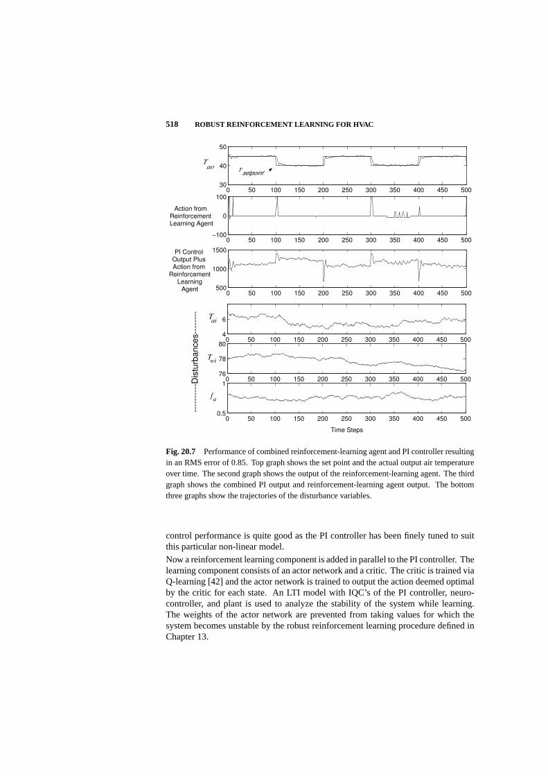
518 ROBUST REINFORCEMENT LEARNING FOR HVAC
0 50 100 150 200 250 300 350 400 450 50030
40
50
0 50 100 150 200 250 300 350 400 450 500−100
0
100
0 50 100 150 200 250 300 350 400 450 500500
1000
1500
Tao
Tsetpoint
Action from Reinforcement Learning Agent
PI Control Output Plus Action from
Reinforcement Learning
Agent
0 50 100 150 200 250 300 350 400 450 5004
6
0 50 100 150 200 250 300 350 400 450 50076
78
80
0 50 100 150 200 250 300 350 400 450 5000.5
1
Tai
Twi
fa
Time Steps
----
----
--D
istu
rba
nce
s--
----
--
Fig. 20.7 Performance of combined reinforcement-learning agent and PI controller resultingin an RMS error of 0.85. Top graph shows the set point and the actual output air temperatureover time. The second graph shows the output of the reinforcement-learning agent. The thirdgraph shows the combined PI output and reinforcement-learning agent output. The bottomthree graphs show the trajectories of the disturbance variables.
control performance is quite good as the PI controller has been finely tuned to suitthis particular non-linear model.
Now a reinforcement learning component is added in parallel to the PI controller. Thelearning component consists of an actor network and a critic. The critic is trained viaQ-learning [42] and the actor network is trained to output the action deemed optimalby the critic for each state. An LTI model with IQC’s of the PI controller, neuro-controller, and plant is used to analyze the stability of the system while learning.The weights of the actor network are prevented from taking values for which thesystem becomes unstable by the robust reinforcement learning procedure defined inChapter 13.

ROBUST CONTROL FRAMEWORK FOR COMBINED PI AND RL CONTROL 519
Fig. 20.8 Tracking performance of nominal controller and nominal plus trained neuro-controller. Bottom graph shows output of neuro-controller.
Inputs to both learning components are the tracking error and the three internal statevariables of the non-linear model:Fw, Tao, andTwo. To choose the number of hiddenunits in the actor network, several different configurations were tested. A networkwith a single hidden layer of 10 units was found to perform well. TheQ function isapproximated by a table indexed byFw, Tao, andTwo and the control action. Eachof the four input dimensions is quantized into 10 intervals, resulting in aQ table of104 entries.
The middle graph of Figure 20.8 shows the step responses of the combined PI/RLcontrollers. The output of the actor network is also shown in the bottom graph. Theactor network learns to produce no output control signal for most cases. Only duringa step transition in the reference input, the action network outputs a very small controlsignal to be added to the PI control signal.
The squared tracking error summed over the sequence shown in Figure 20.8 is 0.526when just the PI controller is used. The error is decreased to 0.518 when the RLcontroller is added. This is a slight, 1.5%, decrease in error. The nominal PI controllerprovides fairly good tracking performance, leaving little room for improvement bythe RL controller. This result is significant not for the small improvement achieved
520 ROBUST REINFORCEMENT LEARNING FOR HVAC
by the RL agent, but for the fact the system is guaranteed to be stable throughout theentire learning phase. Details of these results are presented by Kretchmar [26].
The RL controller uses state information that is not available to the PI controller. Byexploiting this extra information, the RL controller may be able to implement bettercontrol performance. However, the addition of more state variables might not alwaysbe the best solution; it may be the case that a better performing controller can be foundby using fewer state variables. The reason for this counter-intuitive relationship isthat the added state information increases the complexity of the feedback loop which,in turn, allows more possibilities for unstable control. This may limit the flexibilityinherent in the RL algorithm in order to guarantee control.
If the PI controller provides excellent control performance, then why consider apply-ing this robust RL scheme to this task? The primary reason involves the differencebetween the real physical plant and the plant model. The dynamics of the plantmodel will be different from the unknown dynamics of the physical system. ThePI controller may still be “tuned” for the physical plant, but the performance of thiscontroller is expected to be substantially less than the performance of the PI controlleron the plant model. Essentially, there is likely to be more room for improved controlperformance when the physical plant is involved.
20.5 CONCLUSIONS
Two experiments are described in augmenting PI controllers with reinforcementlearning (RL) agents to learn improved control of a non-linear model of a heatingcoil. In the first experiment, the combined PI and RL controllers were applied to athe heating coil. The RL agent was trained using a Q-learning algorithm to form atabular approximation to the optimal Q function. Results show that the reinforcementlearning agent learns to modify the PI controller’s output only at times when the PIcontroller is not adequate to meet performance objectives.
For the second experiment, the heating coil model is linearized to enable the ap-plication of robust stability analysis to the control system, including the RL agent.This required the addition of an artificial neural network as an action network to theRL agent. The resulting system was then trained with stability constraints in effect.The results show that a small amount of performance improvement occurred withthe addition of the RL agent. More importantly, learning occurred in the context ofguaranteed stability.
It is hypothesized that performance improvements achieved with RL agents would bemuch more substantial in a real heating coil due to uncertainties and non-linearitiesthat are present in real systems. These uncertainties and non-linearities result inconservative robust controllers, whose performance can be improved by RL agentsbeing fine-tuned through interactions with the real system. A physical heating coilwith many sensors and actuators is being constructed at Colorado State Universityto research this question. The status of this project is summarized at the web sitehttp://www.engr.colostate.edu/nnhvac.

CONCLUSIONS 521
Acknowledgments
This work was supported by the National Science Foundation through grants CMS-9401249and CISE-9422007.
Bibliography
1. O. Ahmed, J. W. Mitchell, and S. A. Klein, “Application of general regressionneural network (GRNN) in HVAC process identification and control,”ASHRAETransactions,vol. 102, pt. 1, 1996.
2. C. W. Anderson, D. C. Hittle, A. D. Katz, and R. M. Kretchmar, “Synthesis ofreinforcement learning, neural networks, and pi control applied to a simulatedheating coil,”Artificial Intelligence in Engineering,11(4):423–431, 1997.
3. G. J. Balas, and P. M. Young, “Control Design for Variations in StructuralNatural Frequencies,”AIAA Journal of Guidance, Dynamics and Control,vol. 18,pp. 325–332, 1995.
4. G. J. Balas, A. K. Packard, J. C. Doyle, K. Glover, and R. S. Smith, “Developmentof advanced control design software for researchers and engineers,”Proceedingsof the American Control Conference,pp. 996–1001, 1991.
5. B. Bamieh and M. Dahleh, “Robust stability with structured time-invariant per-turbations,”Proceedings of the 31st IEEE Conference on Decision and Control,pp. 1987–1990, 1992.
6. B. R. Barmish, and H. I. Kang, “A survey of extreme point results for robustnessof control systems,”Automatica,vol. 29, pp. 13-35, 1993.
7. E. Bass, and K. Y. Lee, “Robust control of nonlinear systems using norm-boundedneural networks,”Proceedings of the 1994 IEEE International Conference onNeural Networks,pp. 2524–2529, 1994.
8. J. Bekker, P. K. Meckel, and D. Hittle, “A tuning method for first order processeswith PI controllers,”ASHRAE Transactions,vol. 97, pt. 1, 1991.
9. S. Brandt, “Adaptive control implementation issues,”ASHRAE Transactions,vol. 92, pt. 2B, pp. 211–219, 1986.
10. H. Buschek, and A. J. Calise, “Hypersonic flight control system design usingfixed order robust controllers,”6th International Aerospace Planes and Hyper-sonic Technologies Conference, 1995.
522
BIBLIOGRAPHY 523
11. K. D. Cock, B. D. Moor, W. Minten, W. V. Brempt, and H. Verrelst, “A tutorial onPID-control,” Technical Report ESAT-SIST/TR 1997-08, Katholieke UniversiteitLeuven, 1997.
12. P. S. Curtiss, “Experimental results from a network-assisted PID controller,”ASHRAE Transactions,vol. 102, pt. 1, 1996.
13. P. S. Curtiss, J. K. Kreider, and M. J. Brandemuehl, “Adaptive control of HVACprocesses using predictive neural networks,”ASHRAE Transactions,vol. 99,pt. 1, 1993.
14. P. S. Curtiss, G. Shavit, and J. K. Kreider, “Neural networks applied tobuildings—a tutorial and case studies in prediction and adaptive control,”ASHRAE Transactions,vol. 102, pt. 1, 1996.
15. A. Dexter, and P. Haves, “A robust self-tuning predictive controller for HVACapplications,”ASHRAE Journal,vol. 32, no. 12, pp. 12–22, 1990.
16. J. C. Doyle, “Analysis of feedback systems with structured uncertainty,”IEEEProceedings,Pt. D, vol. 129, pp. 242–250, 1982.
17. J. C. Doyle, “Structured uncertainty in control system design,”Proceedings ofthe 24th Conference on Decision and Control,pp. 260–265, 1985.
18. N. Elia, P. M. Young, and M. A. Dahleh, “Robust Performance for Both Fixed andWorst Case Inputs,”34th IEEE Conference on Decision and Control,pp. 3170–3175, 1995.
19. F. Ferrano, and K. Wong, “Prediction of thermal storage loads using a neuralnetwork,”ASHRAE Transactions,vol. 96, pt. 2, pp. 723–726, 1990.
20. J. S. Haberl, L. K. Norford, and J. V. Spadaro, “Diagnosing building operationalproblems,”ASHRAE Journal,vol. 31, no. 6, pp. 20–30, 1989.
21. S. J. Hepworth, and A. L. Dexter, “Neural control of non-linear HVAC plant,”Proceedings of the IEEE Conference on Control Applications,vol. 3, pt. 3,pp. 1849–1854, 1994.
22. P. A. Ioannou, and J. Sun,Robust Adaptive Control,Prentice Hall, New Jersey,1996.
23. M. Khammash, and J. B. Pearson, “Performance robustness of discrete-timesystems with structured uncertainty,”IEEE Transactions on Automatic Control,vol. 36, pp. 398–412, 1991.
24. A. Megretsky, “Necessary and sufficient conditions of stability: A multiloopgeneralization of the circle criterion,”IEEE Transactions on Automatic Control,vol. 38, pp. 753–760, 1993.
524 BIBLIOGRAPHY
25. R. Miller, and J. Seem, “Comparison of artificial neural networks with traditionalmethods of predicting return time from night or weekend setback,”ASHRAETransactions,vol. 97, 1991.
26. R. M. Kretchmar,A Synthesis of Reinforcement Learning and Robust ControlTheory,PhD thesis, Colorado State University, Department of Computer Sience,2000.
27. C. G. Nesler, and W. F. Stoecker, “Selecting the proportional and integral con-stants in the direct digital control of discharge air temperature,”ASHRAE Trans-actions,vol. 90, pt. 2B, pp. 834-845, 1984.
28. L. K. Norford, A. Allgeier, and J. V. Spadaro, “Improved energy information fora building operator—exploring the possibilities of a quasi-real-time knowledge-based system,”ASHRAE Transactions,vol. 96, pt. 1, pp. 1515–1523, 1990.
29. F. Paganini, “Necessary and Sufficient Conditions for RobustH2 Performance,”American Control Conference,pp. 1970–1975, 1995.
30. M. Pinella, D. C. Hittle, E. Wechselberger, and C. Pederson, “Self-tuning digitalintegral control,”ASHRAE Transactions,vol. 92, pt. 2B, pp. 202–209, 1986.
31. M. G. Safonov, “Stability margins for diagonally perturbed multivariable feed-back systems,”IEEE Proceedings,Pt. D, vol. 129, pp. 251-256, 1982.
32. J. E. Seem, “A new pattern recognition adaptive controller,” Presented at 13thInternational Federation of Automatic Control World Congress, 1996.
33. J. Seem, and J. Braun, “Adaptive methods for real-time forecasting of buildingelectrical demand,”ASHRAE Transactions,vol. 97, 1991.
34. J. E. Seem, and H. J. Haugstad, “Field and laboratory results for a new patternrecognition adaptive controller,”Proceedings of the CLIMA 2000 InternationalConference,Brussels, Belgium, p. 77, 1997.
35. J. S. Shamma, “Robust stability with time-varying structured uncertainty,”IEEETransactions on Automatic Control,vol. 39, pp. 714–724, 1994.
36. R. S. Sutton, and A. G. Barto,Reinforcement Learning: An Introduction,TheMIT Press, 1998.
37. J. A. K. Suykens, B. L. R. De Moor, and J. Vandewalle, “Nonlinear system iden-tification using neural state space models, applicable to robust control design,”International Journal of Control,pp. 129–152, 1995.
38. D. M. Underwood, and R. R. Crawford, “Dynamic nonlinear modeling of a hot-water-to-air heat exchanger for control applications,”ASHRAE Transactions,97(1):149–155, 1991.

BIBLIOGRAPHY 525
39. P. J. Werbos, “An overview of neural networks for control,”Control Systems,pp. 40-41, 1991.
40. P. M. Young, “Controller Design with Real Parametric Uncertainty,”Interna-tional Journal of Control,vol. 65, pp. 469–509, 1996.
41. P. M. Young, and M. A. Dahleh, “RobustLp Stability and Performance,”Systems& Control Letters,vol. 26, pp. 305–312, 1995.
42. C. Watkins,Learning with Delayed Rewards,PhD thesis, Cambridge UniversityPsychology Department, Cambridge, England, 1989.
21 Helicopter Flight Control UsingDirect Neural DynamicProgramming
RUSSELL ENNS and JENNIE SI
Arizona State University
Editor’s Summary: This chapter presents a complex continuous state systemcontrol problem using the direct NDP method introduced in Chapter 5. The systemexamined is an Apache helicopter modeled using the full-scale industrial simulatorFLYRT. The focus is on how direct NDP can be used to control complex, realistic, andhigh-dimensional systems. The problem formulation, objectives, implementation,results, and insights that can be gained from doing direct NDP designs are discussedin detail. This case study is one of the applications examined in this book that addressthe challenging generalization issue.
21.1 INTRODUCTION
Generalization or scalability of an approximate dynamic programming methodologyto large and complex problems is one of the major challenges to date. This chapterfocuses on demonstrating that the direct neural dynamic programming (direct NDP)method introduced in Chapter 5 can be successfully applied to complex, realistic,higher dimensional systems. Furthermore it shows the promise of direct NDP as arobust approximate dynamic programming control system design technique based onmeasures such as learning statistics, problem scalability, and the range of problemshandled.
In this chapter the original direct NDP mechanism presented in [11] is expanded onin order to improve its learning ability. Then, a comprehensive case study of this newdesign is presented. The example used is helicopter flight control, where the controlgoals are to perform both helicopter stabilization and maneuvering for a full-scaleindustrial helicopter model. The model is quite complex, being both highly nonlinearand having multiple inputs and multiple outputs (MIMO).
526
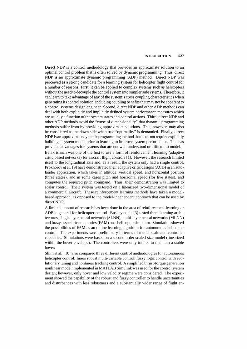
INTRODUCTION 527
Direct NDP is a control methodology that provides an approximate solution to anoptimal control problem that is often solved by dynamic programming. Thus, directNDP is an approximate dynamic programming (ADP) method. Direct NDP wasperceived as a strong candidate for a learning system for helicopter flight control fora number of reasons. First, it can be applied to complex systems such as helicopterswithout the need to decouple the control system into simpler subsystems. Therefore, itcan learn to take advantage of any of the system’s cross coupling characteristics whengenerating its control solution, including coupling benefits that may not be apparent toa control systems design engineer. Second, direct NDP and other ADP methods candeal with both explicitly and implicitly defined system performance measures whichare usually a function of the system states and control actions. Third, direct NDP andother ADP methods avoid the “curse of dimensionality” that dynamic programmingmethods suffer from by providing approximate solutions. This, however, may alsobe considered as the down side when true “optimality” is demanded. Finally, directNDP is an approximate dynamic programming method that does not require explicitlybuilding a system model prior to learning to improve system performance. This hasprovided advantages for systems that are not well understood or difficult to model.
Balakrishnan was one of the first to use a form of reinforcement learning (adaptivecritic based networks) for aircraft flight controls [1]. However, the research limiteditself to the longitudinal axis and, as a result, the system only had a single control.Prokhorov et al. [9] have demonstrated their adaptive critic designs (ACD) in an auto-lander application, which takes in altitude, vertical speed, and horizontal position(three states), and in some cases pitch and horizontal speed (for five states), andcomputes the required pitch command. Thus, their demonstration was limited toscalar control. Their system was tested on a linearized two-dimensional model ofa commercial aircraft. These reinforcement learning methods have taken a model-based approach, as opposed to the model-independent approach that can be used bydirect NDP.
A limited amount of research has been done in the area of reinforcement learning orADP in general for helicopter control. Buskey et al. [3] tested three learning archi-tectures, single layer neural networks (SLNN), multi-layer neural networks (MLNN)and fuzzy associative memories (FAM) on a helicopter simulator. Simulation showedthe possibilities of FAM as an online learning algorithm for autonomous helicoptercontrol. The experiments were preliminary in terms of model scale and controllercapacities. Simulations were based on a second order scaled-size model (linearizedwithin the hover envelope). The controllers were only trained to maintain a stablehover.
Shim et al. [10] also compared three different control methodologies for autonomoushelicopter control: linear robust multi-variable control, fuzzy logic control with evo-lutionary tuning and nonlinear tracking control. A simplified thrust-torque generationnonlinear model implemented in MATLAB Simulink was used for the control systemdesign; however, only hover and low velocity regime were considered. The experi-ment showed the capability of the robust and fuzzy controller to handle uncertaintiesand disturbances with less robustness and a substantially wider range of flight en-

528 HELICOPTER FLIGHT CONTROL USING DIRECT NDP
velopes covered by nonlinear control with more accurate system knowledge needed.However, the research was limited to near hover conditions and simplified systemuncertainties and disturbances.
Bagnell and Schneider [2] used policy search methods to fly an autonomous he-licopter. After the dynamical system was sampled to build a LWBR state-spacemodel, the policy search method was then applied to evaluate and synthesize simpleone-layer neural network controllers under distributions of the identified Markovianmodels towards a pre-defined cost criterion. The method was validated for the CIFERsystem developed by the U.S. Army, although only the so-called “core dynamics”of the helicopter were considered. The control was limited to the longitudinal andlateral axis and, as a result, the system only had two controls. The controller wastrained to regulate the helicopter hovering about a point or a slowly varying trajectory.
Wan et al. [12] developed a model predictive neural control (MPNC) system whichcombines the conventional neural network (NN) control and the nonlinear state-dependent Riccati equation (SDRE) control for aggressive helicopter maneuvers.The SDRE controller design, repeated at every sample time, provided initial localasymptotic stability. The neural network controller was optimized by learning theweights to minimize the receding horizon MPC cost function. The NN controller waspre-trained to behave similar to the SDRE controller, updated online for every N timesteps where N is the receding horizon time with weights from the previous horizonused as the initialization. During the training, the SDRE controller provided stabletracking and good conditions, while the NN decreased the tracking error. The MPNCcontroller augmented the SDRE controller with the NN controllers by a relativeweighting constant. As training progressed, the SDRE control reduced, which in turngave more authority to the neural controller. Simulation was based on a helicoptermodel built via a simulation package called FlightLab. A twelve dimensional statevector was used with four control outputs. Various maneuvers such as rapid take-offand landings and “elliptic” maneuvers were simulated. Simulation results showed theimproved performance over traditional SDRE and LQ control. However, their systemwas still constrained in the following two ways. First, their system took a model-based approach, as opposed to the model-independent approach used by other onlinelearning algorithms. The SDRE controller required an analytical approximation ofthe system dynamics which meant a system model needed to be identified to generatethe SDRE control. Therefore, issues like model mismatch would certainly affectthe final controller performance. Second, the computational effort was extensive. ARiccati equation needed to be solved at every iteration. The Jacobians for the flightsystem also needed to be evaluated via perturbation during backward simulation fortraining the NN network. With current CPU speeds, this approach is precluded fromuse in real-time control.
The purpose of this research is not to compare the direct NDP method to any ofthe existing methods, be they reinforcement learning based, neural network basedor otherwise. Rather, the purpose is to demonstrate the power of direct NDP as anapproximate dynamic programming control methodology on a challenging controlsproblem that other approximate dynamic programming algorithms may not be able

THE HELICOPTER MODEL 529
to handle. This is done by first showing how direct NDP can be used to stabilizea helicopter for five flight conditions (hover, 30, 60, 90 and 120 knots), and thenshowing how it can learn to perform a number of aircraft maneuvers (hover to 50ft/s at various accelerations, up to the aircraft upper limits of 0.25 g (8ft/s2); anddeceleration maneuvers from 100 ft/s to 50 ft/s at various decelerations). Simulationsare performed in both clear air and in the presence of turbulence and step gusts usingan industrial Dryden model. It is then shown how direct NDP can be used forhelicopter flight control reconfiguration, demonstrating the possibility of using directNDP to control the helicopter even in the presence of an actuator failure. Thisshows the promise of direct NDP as a useful reinforcement learning method in thefailure accommodation realm. Unlike many results which are based on linearizedmodels and corresponding assumptions, these direct NDP designs and simulationsare conducted using FLYRT, a very realistic nonlinear system model.
The chapter is organized as follows. Section 21.2 briefly describes the helicoptermodel used for evaluating the direct NDP designs. Section 21.3 then expands onthe direct NDP methodology developed in Chapter 5 and applies it to the helicopterflight control stabilization problem. Key to this expanded direct NDP methodologyis the trim network which is crucial to the success of direct NDP for complex non-linear systems. The direct NDP methodology is then further refined for the morecomplicated helicopter command tracking and reconfigurable flight control problemsin Sections 21.4 and 21.5 and simulation results are presented. Section 21.6 thenprovides some conclusions.
21.2 THE HELICOPTER MODEL
A helicopter is a sophisticated system with multiple inputs used to control a significantnumber of states. There exists a large amount of cross coupling between controlinputs and states. Further, the system is highly non-linear and changes significantlyas a function of operating condition. For these reasons the helicopter serves as anexcellent and challenging platform for testing approximate dynamic programmingsystems.
The helicopter’s states are controlled by a main rotor and a tail rotor. There arethree main rotor actuators whose positions,zA, zB , andzC , control the position andorientation of a swash plate which in turn controls the main rotor’s blade angles asa function of rotational azimuth. There is a single tail rotor actuator position (zD)which controls the tail rotor’s blade angles. The aircraft states are numerous. Forflight control purposes the states of interest are the aircraft translational (u, v, w) androtational (p, q, r) velocities and the aircraft orientation (θ, φ, ψ) for a total of ninestates. The helicopter’s longitudinal (u), lateral (v), and vertical velocities (w) are inft/s. The helicopter’s roll rate (p), pitch rate (q), and yaw rate (r) are in degrees/s.The helicopter’s Euler angles, pitch (θ), roll (φ) and yaw (ψ) are in degrees. Thestates can be written in vector form asx = [u, v, w, p, q, r, θ, φ, ψ]. The controls canbe written in vector form asu = [zA, zB , zC , zD].

530 HELICOPTER FLIGHT CONTROL USING DIRECT NDP
MAINEXECUTIVE
TRIMMODULE
LINEAR MODELMODULE
FLYRT MODULE- MAIN ROTOR MODULE- FUSELAGE MODULE- HORIZ. STAB. MODULE- TAIL ROTOR/VERT. MODULE- LANDING GEAR MODULE- ENGINE MODULE
EQUATIONSOF MOTION
INTEGRATIONMODULE
Fig. 21.1 Major Components of Helicopter Model
For simulation purposes a detailed helicopter model run at 50 Hz is used to evaluatethe direct NDP controller’s performance. The model, named FLYRT and shown inFigure 21.1, is a sophisticated nonlinear helicopter flight simulation model developedover the past two decades [8]. FLYRT models all the forces and moments actingon the helicopter. The rotor is modeled using a blade element model. FLYRTdynamically couples the six-degrees-of-freedom rigid body of the helicopter to themain rotor through Euler equations. The drive train is represented as a single degreeof freedom model and is coupled to the main rotor, tail rotor and engine. The engineis modeled in sufficient detail to cover performance over all phases of flight, includingground modes. The landing gear is modeled as three independent units interfacingwith a rigid airframe. Quaternions are used during state integration to accommodatelarge attitude maneuvers.
FLYRT also models the mechanical geometry between the actuators and the helicopterblades as well as the dynamics of the actuators. Each actuator is modeled as a firstorder lag with time constantτ = 0.03, reflective of a typical actuator. Actuator rateand position limits are also modeled.
The Apache helicopter is the helicopter modeled for the simulation studies. Theoperating conditions for which the studies are performed are shown in Table 21.1.The center of gravity (C.G.) is listed in the standard Apache FS/WL/BL coordinateframe [8].
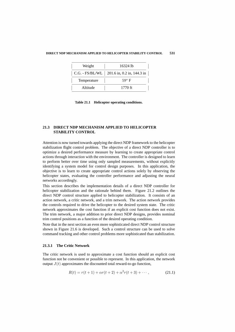
DIRECT NDP MECHANISM APPLIED TO HELICOPTER STABILITY CONTROL 531
Weight 16324 lb
C.G. - FS/BL/WL 201.6 in, 0.2 in, 144.3 in
Temperature 59o F
Altitude 1770 ft
Table 21.1 Helicopter operating conditions.
21.3 DIRECT NDP MECHANISM APPLIED TO HELICOPTERSTABILITY CONTROL
Attention is now turned towards applying the direct NDP framework to the helicopterstabilization flight control problem. The objective of a direct NDP controller is tooptimize a desired performance measure by learning to create appropriate controlactions through interaction with the environment. The controller is designed to learnto perform better over time using only sampled measurements, without explicitlyidentifying a system model for control design purposes. In this application, theobjective is to learn to create appropriate control actions solely by observing thehelicopter states, evaluating the controller performance and adjusting the neuralnetworks accordingly.
This section describes the implementation details of a direct NDP controller forhelicopter stabilization and the rationale behind them. Figure 21.2 outlines thedirect NDP control structure applied to helicopter stabilization. It consists of anaction network, a critic network, and a trim network. The action network providesthe controls required to drive the helicopter to the desired system state. The criticnetwork approximates the cost function if an explicit cost function does not exist.The trim network, a major addition to prior direct NDP designs, provides nominaltrim control positions as a function of the desired operating condition.
Note that in the next section an even more sophisticated direct NDP control structureshown in Figure 21.6 is developed. Such a control structure can be used to solvecommand tracking and other control problems more sophisticated than stabilization.
21.3.1 The Critic Network
The critic network is used to approximate a cost function should an explicit costfunction not be convenient or possible to represent. In this application, the networkoutputJ(t) approximates the discounted total reward-to-go function,
R(t) = r(t + 1) + αr(t + 2) + α2r(t + 3) + · · · , (21.1)

532 HELICOPTER FLIGHT CONTROL USING DIRECT NDP
uNN1(t)
J(t)
x*(t)
J(t-1)-r(t) Uc(t)
Action
Network
(Off-line)
Critic
Network
No
rmalizer
x(t)
x*2(t)
+
-
+
-
x(t)
Kcont
xd(t)
-
+
Action
Network
(On-line)
Klmtd
Trim
Position
Network
+
+
+
xd(t)
env. parameters
uNN2(t)
utrim(t)
u(t) Helicopter
Simulation
Fig. 21.2 Direct NDP based helicopter controller for stabilization, featuring simple actionnetwork, trim network, and critic network.
whereR(t) is the future accumulative reward-to-go value at timet, α is a discountfactor for the infinite-horizon problem (0 < α < 1), andr(t) is the external rein-forcement value at timet.
In prior direct NDP research,r(t) was simply a binary reinforcement signal givenby r(t) = 0 if successful, orr(t) = −1 if failure occurs at the end of an event. Forthis application, a more informative quadratic reinforcement signal at each samplingtime is formulated
r(t) = −n∑
i=1
((xi − xi,d)
xi,max
)2
(21.2)
wherexi is theith state of the state vectorx, xi,d is the desired reference state andxi,max is the nominal maximum state value.
The critic network is implemented with a standard multi-layer nonlinear feed-forwardneural network as shown in Chapter 5. A sigmoid function is used for the nonlinearity.The inputs to the critic network are all states, normalized and squared. The output isthe approximate cost functionJ(t). The technique for training this critic network isshown in Chapter 5.
21.3.2 The Action Network
The action network generates the desired plant control given measurements of theplant states. As with the critic network, the action network is implemented with astandard multi-layer nonlinear feed-forward neural network. The number of networkoutputs equals the control space dimension.
DIRECT NDP MECHANISM APPLIED TO HELICOPTER STABILITY CONTROL 533
The principle in adapting the action network is to back-propagate the error betweenthe desired ultimate objective, denoted byUc, and the total reward-to-goR(t). Uc
is usually set to 0 since success was defined to be 0. Either the actual total rewardfunctionR(t), or an approximation to itJ(t), is used depending on whether an explicitcost function or a critic network is available. In the latter case back-propagation isdone through the critic network. Training of the action network is provided in Chapter5.
If desired, a second action network can be implemented to perform on-line learning toadapt to local flight conditions while the first action network’s weights are frozen afterhaving been trained off-line under specific common flight conditions. The secondnetwork’s on-line weight adaptations based on its experiences should improve thecontroller’s performance. It can be authority limited as required by the application.The results in this paper do not include the second aritifical neural network (ANN).
21.3.3 The Trim Network
The trim (position) network is a neural network, or lookup table, that is trained,or programmed, to schedule the aircraft’s nominal actuator position and aircraftorientation as a function of operating conditions. This section describes the conceptof trim, explains why it is a critical element in nonlinear flight control system design,and provides an overview of a method for determining trim. Further details of thedevelopment of the trim network can be found in [5]. This trim method, thoughapplied to helicopters here, can be extended to any general control system.
Controlling the helicopter is a nonlinear control system design problem. An importantpart of nonlinear control system design, often not discussed, is the ability to determinethe trim states for the system (e.g. helicopter) over all operating conditions. The trimstates are the positions of the controls and the dependent system states associatedwith achieving a desired steady state condition. When the system is trimmed, thechange in state derivative (e.g. acceleration) is either zero or minimized.
For example, with an aircraft one tries to adjust (trim) the controls to balance theaerodynamic, inertial and gravitational forces and moments in all axes at all times.The aircraft is trimmed when the desired balance is achieved or the aircraft enters adesired steady state. In the case of a helicopter, the controls to be trimmed are thefour actuators and the dependent states to be trimmed are the pitch, roll and yaw, i.e.,seven trim state variables in total. These states are trimmed for the desired specifiedsteady state translational velocities (u, v, w) and angular rates (p, q, r), i.e., sixvariables representing desired steady states.
When flying a conventional mechanically controlled helicopter, a pilot continuallytrims the helicopter via his closed loop control. Similarly, traditional PID basedcontrol techniques inherently trim the helicopter, the integrators serve as the trimcomponent. The ability to incorporate a trim ability into direct NDP is paramountto successfully applying direct NDP to the helicopter control problem. It serves asa good first guess at the required control solution, turning the global optimizationproblem into a local optimization problem. Previous direct NDP control designs

534 HELICOPTER FLIGHT CONTROL USING DIRECT NDP
were successful because the systems that were tested (e.g. the inverted pendulum)had a zero trim requirement [11]. Similarly, many flight control papers have assumedlinear models in which case there is also a zero trim requirement since the model islinearized about a trim condition. In both cases, the problem definition implicitlymakes it a local optimization problem.
Trimming requires determining the seven trim state variables to include four controlpositions (u) and three body angles (defined below to bex2) for a given flightcondition. For this reason, the original state vectorx is divided into two parts,x1 = [u, v, w, p, q, r] andx2 = [θ, φ, ψ], wherex1 represents the desired steady statevariables for which the seven trim positions,[utrim x2
trim], are to be determined.
Figure 21.3 shows the neural network structure used to determine the seven aircrafttrim positionsutrim and x2
trim for any desired trim steady statex1trim. The
trim network is a one-layer weight feed-forward network with seven biases (b) thatcorrespond to the seven trim states. The network has a nonlinear sigmoid functionfanning out the outputs. In using the action network for trim, the inputs to the trimnetwork are zeroed and there are seven outputs from the network including fourcontrols and three body angles.
utrimOne-layer
weight
feed-forward
network
Helicopter
Simulation0
x(t)Kcont
Cost
Function
Jt(t)
trim2x Kcont
Fig. 21.3 Neural network structure for determining trim. The objective is to mininimize thespecified cost functionJt(t).
State equations associated with Figure 21.3 are as follows.
[utrim x2trim] = fsig(b), (21.3)
wherefsig(b) = [fsig(b1), · · · , fsig(b7)], (21.4)
andfsig(ξ) = 2(1− e−ξ)/(1 + e−ξ). (21.5)
The cost function used isJt = 1/2xT x, wherexi = (x1i−x1
trim,i)x1
max,i, i = 1, · · · , 6.
The basic technique for determining the trim positions is to train the network, whoseinputs are zeroed and that has biases, to minimize the cost function. After training iscomplete, the resulting biases then provide the aircraft trim positions. The weightsin this network are of no importance other than the bias vector. This trim network istrained over a number of epochs where in each epoch,m, the plant model is initialized,
DIRECT NDP MECHANISM APPLIED TO HELICOPTER STABILITY CONTROL 535
the plant dynamics are evolved for a specified timetf , and back-propagation isperformed to adjust the trim network biases to minimize the objective at timetf forthat epoch,m. In general, the variable,v at timetf for epochm, is denoted asv(m).For example, the objective function at timetf for epochm is denotedJt(m).The network biases,b, are trained using the same gradient descent training methoddescribed for direct NDP. That is,
b(m + 1) = b(m) + ∆b(m), (21.6)
∆bi(m) = λ(m)[−∂Jt(m)
∂bi(m)
], i = 1 . . . 7, (21.7)
whereλ is the learning rate. For the four biases corresponding to the trim controls
∂Jt(m)∂bi(m)
=∂Jt(m)∂x1(m)
∂x1(m)∂u(m)
∂u(m)∂bi(m)
, i = 1 . . . 4. (21.8)
For the three biases corresponding to the trim body angles
∂Jt(m)∂bi(m)
=∂Jt(m)∂x1(m)
∂x1(m)∂x2(m)
∂x2(m)∂bi(m)
, i = 5 . . . 7. (21.9)
In both cases the first partial is evaluated in the manner described earlier in the direct
NDP mechanism. For the trim angles bias updates, the partials∂x1(m)∂x2(m) and∂x1(m)
∂u(m) canbe calculated numerically via perturbations to the system. Alternatively, the partial∂x1(m)∂x2(m) can be approximated analytically at hover from simple physics (rotate thegravity vector into the body frame and use appropriate small angle approximations).The partials are computed at hover only and used for all flight conditions for theresults presented.
Once training is complete the trim positions are then determined from the networkbiases via the sigmoid function. Note that the trim network is trained off-line first,independent of the action and the critic networks in the direct NDP controller.
21.3.4 Other Considerations
Several other considerations need to be made in order to implement the direct NDPcontroller for control of sophisticated systems such as a helicopter. First, the actionnetwork is implemented as a traditional two-layer feed-forward network. However,since the action neural network’s output (control) is typically limited to±1 by thesigmoidal non-linearity present in the last stage of the network, a control scalingfactor is used for each control. The value chosen is typicallyKcont = umax whereumax is the maximum control authority of the actuators. It is necessary to incorporatethis scaling into the back-propagation when training the action network.
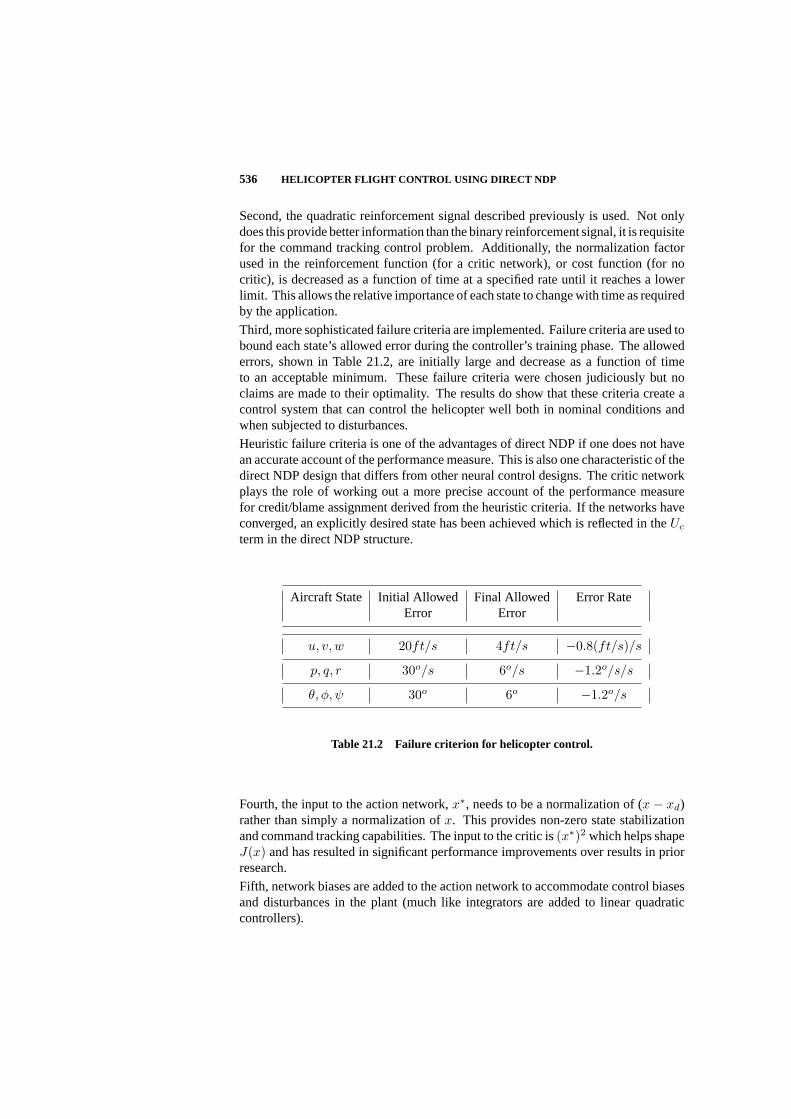
536 HELICOPTER FLIGHT CONTROL USING DIRECT NDP
Second, the quadratic reinforcement signal described previously is used. Not onlydoes this provide better information than the binary reinforcement signal, it is requisitefor the command tracking control problem. Additionally, the normalization factorused in the reinforcement function (for a critic network), or cost function (for nocritic), is decreased as a function of time at a specified rate until it reaches a lowerlimit. This allows the relative importance of each state to change with time as requiredby the application.
Third, more sophisticated failure criteria are implemented. Failure criteria are used tobound each state’s allowed error during the controller’s training phase. The allowederrors, shown in Table 21.2, are initially large and decrease as a function of timeto an acceptable minimum. These failure criteria were chosen judiciously but noclaims are made to their optimality. The results do show that these criteria create acontrol system that can control the helicopter well both in nominal conditions andwhen subjected to disturbances.
Heuristic failure criteria is one of the advantages of direct NDP if one does not havean accurate account of the performance measure. This is also one characteristic of thedirect NDP design that differs from other neural control designs. The critic networkplays the role of working out a more precise account of the performance measurefor credit/blame assignment derived from the heuristic criteria. If the networks haveconverged, an explicitly desired state has been achieved which is reflected in theUc
term in the direct NDP structure.
Aircraft State Initial Allowed Final Allowed Error RateError Error
u, v, w 20ft/s 4ft/s −0.8(ft/s)/s
p, q, r 30o/s 6o/s −1.2o/s/s
θ, φ, ψ 30o 6o −1.2o/s
Table 21.2 Failure criterion for helicopter control.
Fourth, the input to the action network,x∗, needs to be a normalization of (x − xd)rather than simply a normalization ofx. This provides non-zero state stabilizationand command tracking capabilities. The input to the critic is(x∗)2 which helps shapeJ(x) and has resulted in significant performance improvements over results in priorresearch.
Fifth, network biases are added to the action network to accommodate control biasesand disturbances in the plant (much like integrators are added to linear quadraticcontrollers).
DIRECT NDP MECHANISM APPLIED TO HELICOPTER STABILITY CONTROL 537
21.3.5 Helicopter Stabilization Control Results
The first helicopter flight control goal to consider is that of stabilization. In sta-bilization, the goal is to maintain the aircraft’s desired longitudinal velocity whilemaintaining zero lateral and vertical velocity and zero angular rates. To show ro-bustness, each control goal is tested in three wind conditions: caseA) no wind, caseB) 10 ft/s step gust for 5 seconds, and caseC) turbulence simulated using a Drydenmodel with a spatial turbulence intensity ofσ = 5ft/s and a turbulence scale lengthof LW = 1750ft. Characteristic to prior direct NDP research, the performance ofdirect NDP is summarized statistically. The statistical success of the direct NDPcontroller’s ability to learn to control the helicopter is evaluated for a number ofspecified flight conditions.
For each flight condition 100 runs were performed to evaluate direct NDP’s perfor-mance, where for each run the neural networks’ initial weights were set randomly.Each run consisted of up toN attempts (trials) to learn to successfully control thesystem. An attempt was deemed successful if the helicopter stays within the failurecriteria bounds described in Table 21.2 for the entire flight duration (1 minute). Ifthe controller successfully controled the helicopter withinN trials, the run was con-sidered successful, if not, the run was considered a failure. For stabilization,N was500.
For the 100 runs, the following statistic were collected: the successful run percentage,the average number of trials, and (for command tracking in the following section)the learning deviation. The success percentage reflects the percentage of runs forwhich the direct NDP system successfully learns to control the helicopter. Theaverage number of trials is what it takes the direct NDP system to learn to control thehelicopter. The learning deviation is the standard deviation of the number of trialsfrom run to run. It is used to demonstrate the (in)consistency of the learning controlperformance.
Five flight conditions were considered for direct NDP based helicopter stabilization,the stabilization of the helicopter at hover and at 30, 60, 90 and 120 knots. The sta-tistical success of the direct NDP controller’s ability to learn to control the helicopterwas evaluated for each flight condition. The results are shown in Table 21.3.
The neural network parameters used during training are provided in Table 21.4. Thelearning rates,β, for the action network and critic network were scheduled to decreaselinearly with time (typically over a few seconds). In every time frame the weightequations were updated until either the error had sufficiently converged (E < Etol)or Ncyc internal update cycles of the weights had occurred.Nh was the number ofhidden nodes in the neural networks. Note that these parameters were chosen basedon experience but were not tuned to optimize the results.
Two observations can be made about the results in Table 21.3. First, the resultsindicate that a large number of trials must be made before successful stabilization.This is not suprising for a learning system that learns from experience without anyapriori system knowledge. The ramification is that this training needs to be done off-line (i.e. not in a real helicopter), where failures can be afforded, until the controller

538 HELICOPTER FLIGHT CONTROL USING DIRECT NDP
Condition (knots) Hover 30 60 90 120
Case A Percentage of 100% 100% 100% 100% 100%Successful Runs
Average No. of Trials 18 47 36 30 70
Case B Percentage of 28% 72% 82% 66% 30%Successful Runs
Average No. of Trials 201 148 162 176 191
Case C Percentage of 88% 63% 74% 77% 45%Successful Runs
Average No. of Trials 128 214 206 186 200
Table 21.3 Direct NDP learning statistics for helicopter stabilization for three differentwind conditions.
Parameter α βa(t0) βa(tf ) βc(t0) βc(tf ) Ncyc,a
Value 0.95 0.1 0.1 0.1 0.01 200
Parameter Ncyc,c Etol,a Etol,c Nh Kcont
Value 100 0.005 0.1 6 5.0
Table 21.4 Neural network parameter values used for stabilization.
is successfully trained. Once trained, the neural network weights are frozen and thecontroller structure shown in Figure 21.6 can be implemented in a helicopter. Limitedauthority on-line training can then be performed to improve system performance.
Second, direct NDP’s learning ability appears to be slightly poorer at hover. Thisis speculated to be a phenomenon due to the lack of “persistence of excitation”. Athover, the system states tend to evolve slower than at higher speeds and so there isless state variation (dynamics information) over the trials from which direct NDP canlearn.
Once the system is successfully trained, the action network’s weights are frozenand the system can be tested. Typical and statistical time histories of the systemperformance when tested are shown for a flight at 30 knots in turbulence (Figure21.4) and a flight at 90 knots exposed to a step gust (Figure 21.5). The typical timehistory was a randomly chosen simulation selected from the repertoire of test runs forthat flight condition. The average error and error deviation reflect the Monte Carlosample mean and sample variance over time when testing all of the successfullytrained networks reflected in the statistics shown in Table 21.3 for the specified flight

DIRECT NDP MECHANISM APPLIED TO HELICOPTER TRACKING CONTROL 539
condition. The results show that once the direct NDP controller has been successfullytrained, it can reliably and consistently drive the system to its desired states. Timehistory plots for the other flight conditions are similar.
21.4 DIRECT NDP MECHANISM APPLIED TO HELICOPTERTRACKING CONTROL
Attention is now turned towards refining the direct NDP framework developed in theprevious section for the helicopter flight control command tracking problem. Figure21.6 outlines the direct NDP control structure applied to helicopter tracking control.It is the same as the design in the prior section except that the action network consistsof a structured cascade of artificial neural networks. The explicit structure embeddedin this action network, lacking in the prior direct NDP designs, allows the direct NDPcontroller to more easily learn and take advantage of the physical relationships anddependencies of the system.
Such structure in the action network is similar to classic controllers for helicopters,providing for inner loop body rate control, attitude control and outer loop velocitycontrol. In this way, the explicit relationships between body angular rates, attitudesand translational velocities are taken advantage of. The potential advantage ofthe structured ANN over classic design methodologies is that it permits full cross-axes control coupling that many single-input-single-output (SISO) PID controllerdesigns do not. However, the structured ANN does introduce a level of humanknowledge/expertise to the direct NDP implementation that is not transparent tonon-experts.
It is possible, but rather cumbersome, to show that a classic proportional controller canbe equated to one instance (one set of weights) of the structured ANN if the networknonlinearities are removed (or linearized about the network operating point). Sucha relationship between the two designs can be used to provide a good first guess ofthe action network weights should one want to apply this “expert” knowledge to thelearning system. However, all results presented here were obtained for a learningsystem that was trained from scratch without using any expert knowledge.
To perform command tracking, a desired state vectorxd to be tracked needs to bespecified. For helicopters, it is well established that only four of the states in the statevectorx are explicitly controllable. In this experiment, the velocitiesu, v andw andthe aircraft’s yaw,ψ are the four states to be controlled. The rotational velocities andremaining Euler angles, pitch and roll, are determined by direct NDP to achieve thespecified tracking goal. This new desired tracking vector,x0
d = [ud, vd, wd, ψd], is asubset of the original desired state vectorxd.
Referring to Figure 21.6, the inputs to the first ANN are the longitudinal and lateralvelocity errors,uerr = ud−u andverr = vd−v, respectively. The first ANN outputsare the resulting desired pitch and roll of the helicopter,θd andφd. The inputs to thesecond ANN are the errors in the aircraft attitudes,θerr = θd + θtrim − θ , φerr =φd + φtrim − φ andψerr = ψd − ψ. The second ANN outputs are the desired roll,
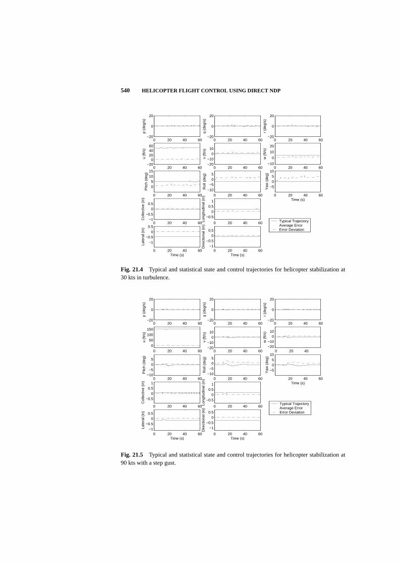
540 HELICOPTER FLIGHT CONTROL USING DIRECT NDP
0 20 40 60−20
0
20
p (d
eg/s
)0 20 40 60
−20
0
20
q (d
eg/s
)
0 20 40 60−20
0
20
r (d
eg/s
)
0 20 40 60−20
0204060
u (f
t/s)
0 20 40 60−20−10
010
v (f
t/s)
0 20 40 60−10
0
10
20
w (
ft/s)
0 20 40 60
05
1015
Pitc
h (d
eg)
0 20 40 60−10
−505
Rol
l (de
g)
0 20 40 60
−505
10
Time (s)
Yaw
(de
g)
0 20 40 60−1
−0.50
0.5
Col
lect
ive
(in)
0 20 40 60
−0.50
0.51
Long
itudi
nal (
in)
0 20 40 60
−1−0.5
00.5
Time (s)
Late
ral (
in)
0 20 40 60−1
−0.50
0.5
Time (s)
Dire
ctio
nal (
in)
Typical TrajectoryAverage Error Error Deviation
Fig. 21.4 Typical and statistical state and control trajectories for helicopter stabilization at30 kts in turbulence.
0 20 40 60−20
0
20
p (d
eg/s
)
0 20 40 60−20
0
20
q (d
eg/s
)
0 20 40 60−20
0
20
r (d
eg/s
)
0 20 40 600
50
100
150
u (f
t/s)
0 20 40 60−20−10
010
v (f
t/s)
0 20 40−20−10
010
w (
ft/s)
0 20 40 60−10
−505
Pitc
h (d
eg)
0 20 40 60−10
−505
Rol
l (de
g)
20 40 60
−505
10
Time (s)
Yaw
(de
g)
0 20 40 60
−0.50
0.51
Col
lect
ive
(in)
0 20 40 60
−0.50
0.51
Long
itudi
nal (
in)
0 20 40 60−1
−0.50
0.5
Time (s)
Late
ral (
in)
0 20 40 60
−1−0.5
00.5
Time (s)
Dire
ctio
nal (
in)
Typical TrajectoryAverage Error Error Deviation
Fig. 21.5 Typical and statistical state and control trajectories for helicopter stabilization at90 kts with a step gust.

DIRECT NDP MECHANISM APPLIED TO HELICOPTER TRACKING CONTROL 541
uNN
J(t)ANN #1
J(t-1)-r(t) Uc(t)
Critic
Network
Helicopter
Simulation
u,v
x*2
+
-
+
-
x = (u,v,w,p,q,r, , ,
Kcont
Cost
Function
J*(t)
ud ,vd
-
+
x*(t)
Trim
Position
Network
+
+
xd0
env. parameters
utrim
u
d , d ANN #2
x* = (x0 -xd0 )/ x0
max
-+
,
trim , trim
+
ANN #3
d
-+
pd ,qd,rd
-
p,q,r
+
wd
-+
w
Cascaded Action Network
x0 = (u,v,w,
Fig. 21.6 Direct NDP based helicopter controller integrating three cascaded artificial neuralnetworks in one action network, a trim network, and a critic network.
pitch and yaw rates (pd, qd, rd) of the helicopter, as a function of the attitude errors.These outputs are then summed with the actual angular rates to obtain the angularrate errors,perr = pd − p, qerr = qd − q andrerr = rd − r. The angular rate errorsand the vertical velocity errorwerr = wd−w then form the inputs to the third ANN.The third ANN then computes the controlsuNN = [uNN,1, uNN,2, uNN,3, uNN,4]as a function of the angular rate and vertical velocity errors. The resultinguNN ,which is normalized because of the ANN structure, is then scaled by the controllerscaling gainKcont and summed with the nominal trim control from the trim network.That is,u = KcontuNN + utrim.
As described in Section 21.3, the objective of the direct NDP controller is to createa series of control actions to optimize a discounted total reward-to-go function.For the helicopter tracking problem we need to define a slightly different quadraticreinforcement signal
r(t) = −n∑
i=1
((x0
i − x0d,i)
x0max,i
)2
(21.10)
where in this applicationn = 4, x0i is thei-th state variable ofx0 = [u, v, w, ψ], and
x0d = [ud, vd, wd, ψd] is the desired state andx0
max,i is a normalization term.
The critic and action networks were then trained per Chapter 5. However, the equa-tions governing the training of the action network were significantly more complexthan prior work since back-propagation must be performed through ANN’s 2 and 3for the training of ANN 1. In essence, it is equivalent to training a six layer networkif each ANN has two-layers of weights. The failure criteria used were the same asthose for stabilization.

542 HELICOPTER FLIGHT CONTROL USING DIRECT NDP
21.4.1 Helicopter Tracking Control Results
This section presents results showing the direct NDP controller’s performance con-trolling the helicopter for a variety of maneuvers. For each maneuver, the controlgoal is for the helicopter to track the desired longitudinal velocity trajectory whilemaintaining zero lateral and vertical velocity and zero steady state angular rates.Statistics were then collected in the same manner as for the helicopter stabilizationcontrol results. The exception was the maximum numer of trials,N , which was 5000for tracking. The parameterN was increased for command tracking because of theincreased complexity of the task compared to stabilization. Since this is a complex,nonlinear, MIMO control system design problem, it provides a good idea of how wellthis ADP algorithm can generalize.
Fourteen maneuvers were considered: seven accelerations from hover to 50 ft/sat various accelerations and seven decelerations from 100 ft/s to 50 ft/s at variousdecelerations. Table 21.5 statistically summarizes the learning ability of the directNDP controller to perform the seven acceleration maneuvers. Results for the sevendeceleration maneuvers are provided in Table 21.6. All maneuvers are conducted foreach of the three wind conditions cited above. The neural network parameters usedduring training for command tracking are provided in Table 21.7.
Cond. Acceleration (ft/s2) 2 3 4 5 6 7 8
Case Success Percentage 94% 62% 67% 65% 66% 66% 74%A Average No. of Trials 1600 2019 2115 1950 1983 2028 1870
Learning Deviation 214 339 324 307 293 306 252
Case Success Percentage 96% 66% 76% 70% 50% 57% 53%B Average No. of Trials 1367 1720 1770 1874 2173 1970 2419
Learning Deviation 191 280 255 275 381 337 400
Case Success Percentage 95% 98% 97% 85% 60% 56% 58%C Average No. of Trials 642 824 1126 1843 1842 2145 2379
Learning Deviation 115 128 165 263 313 333 403
Table 21.5 Learning statistics for hover to 50 ft/s maneuver at various accelerations forthree different wind conditions.
In addition to the tabular learning statistics, both statistical and typical time historyplots of the aircraft states are provided for two cases in the testing phase. Figure 21.7shows both the statistical average state error and error deviation over all successfulruns and a typical plot of the controller performance for a hover to 50 ft/s maneuver atan aggressive5ft/s2 acceleration in the presence of turbulence. Figure 21.8 showsboth the statistical average state error and error deviation and a typical plot of thecontroller performance for a 100 ft/s to 50 ft/s maneuver at4ft/s2 deceleration in
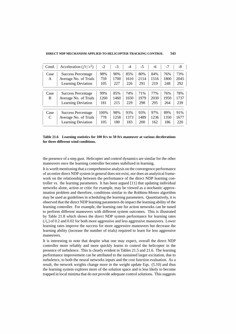
DIRECT NDP MECHANISM APPLIED TO HELICOPTER TRACKING CONTROL 543
Cond. Acceleration (ft/s2) -2 -3 -4 -5 -6 -7 -8
Case Success Percentage 98% 90% 85% 80% 84% 76% 73%A Average No. of Trials 759 1700 1610 2114 1516 1800 2045
Learning Deviation 105 227 226 291 219 248 292
Case Success Percentage 99% 85% 74% 71% 77% 76% 78%B Average No. of Trials 1260 1460 1650 1979 2030 1950 1737
Learning Deviation 181 215 229 298 295 264 239
Case Success Percentage 100% 98% 93% 93% 97% 89% 91%C Average No. of Trials 778 1258 1373 1489 1236 1350 1677
Learning Deviation 105 180 183 200 162 186 220
Table 21.6 Learning statistics for 100 ft/s to 50 ft/s maneuver at various decelerationsfor three different wind conditions.
the presence of a step gust. Helicopter and control dynamics are similar for the othermaneuvers once the learning controller becomes stabilized in learning.
It is worth mentioning that a comprehensive analysis on the convergence performanceof an entire direct NDP system in general does not exist, nor does an analytical frame-work on the relationship between the performance of the direct NDP learning con-troller vs. the learning parameters. It has been argued [11] that updating individualnetworks alone, action or critic for example, may be viewed as a stochastic approx-imation problem and therefore, conditions similar to the Robbins-Monro algorithmmay be used as guidelines in scheduling the learning parameters. Quantitatively, it isobserved that the direct NDP learning parameters do impact the learning ability of thelearning controller. For example, the learning rate for action networks can be tunedto perform different maneuvers with different system outcomes. This is illustratedby Table 21.8 which shows the direct NDP system performance for learning rates(βa) of 0.2 and 0.02 for both more aggressive and less aggressive maneuvers. Lowerlearning rates improve the success for more aggressive maneuvers but decrease thelearning ability (increase the number of trials) required to learn for less aggressivemaneuvers.
It is interesting to note that despite what one may expect, overall the direct NDPcontroller more reliably and more quickly learns to control the helicopter in thepresence of turbulence. This is clearly evident in Tables 21.5 and 21.6. The learningperformance improvement can be attributed to the sustained larger excitation, due toturbulence, to both the neural networks inputs and the cost function evaluation. As aresult, the network weights change more in the weight update Eqs. (5.10) and thusthe learning system explores more of the solution space and is less likely to becometrapped in local minima that do not provide adequate control solutions. This suggests

544 HELICOPTER FLIGHT CONTROL USING DIRECT NDP
that in applications where turbulence or other excitation is not natural, it may beprudent to create an artificial equivalent in order to improve learning performance.
Also note that, as with the stabilization results, a large number of trials must occurto successfully learn to perform the maneuver. Further, the more aggressive themaneuver (the higher the acceleration), the more trials that are required. Again,the ramification is that this training needs to be done done off-line (i.e. not in areal helicopter), where failures can be afforded, until the controller is successfullytrained. Once trained, the neural network weights are frozen and the controllercan be implemented in a helicopter. Limited authority on-line training can then beperformed to improve system performance.
Parameter α βa(t0) βa(tf ) βc(t0) βc(tf ) Ncyc,a
Value 0.95 0.02 0.02 0.1 0.01 200
Parameter Ncyc,c Etol,a Etol,c Nh Kcont
Value 100 0.005 0.1 6 2.5
Table 21.7 Neural network parameter values used for command tracking.
βa Acceleration (ft/s2) 2 6 8
0.02 Success Percentage 94% 66% 74%Average No. of Trials 1600 1983 1870
Learning Variance 214 293 252
0.2 Success Percentage 100% 80% 20%Average No. of Trials 248 1708 2809
Learning Variance 71 421 439
Table 21.8 Learning statistics for hover to 50 ft/s maneuvers as a function of learningrate.
21.5 RECONFIGURABLE FLIGHT CONTROL
Reconfigurable flight control (RFC) is the ability of a helicopter flight control systemto reconfigure itself so that when a failure occurs, for example an actuator is dam-aged or fails, control of the helicopter remains. Such reconfigurable flight controlhas been widely demonstrated on fixed-wing aircraft, taking advantage of control
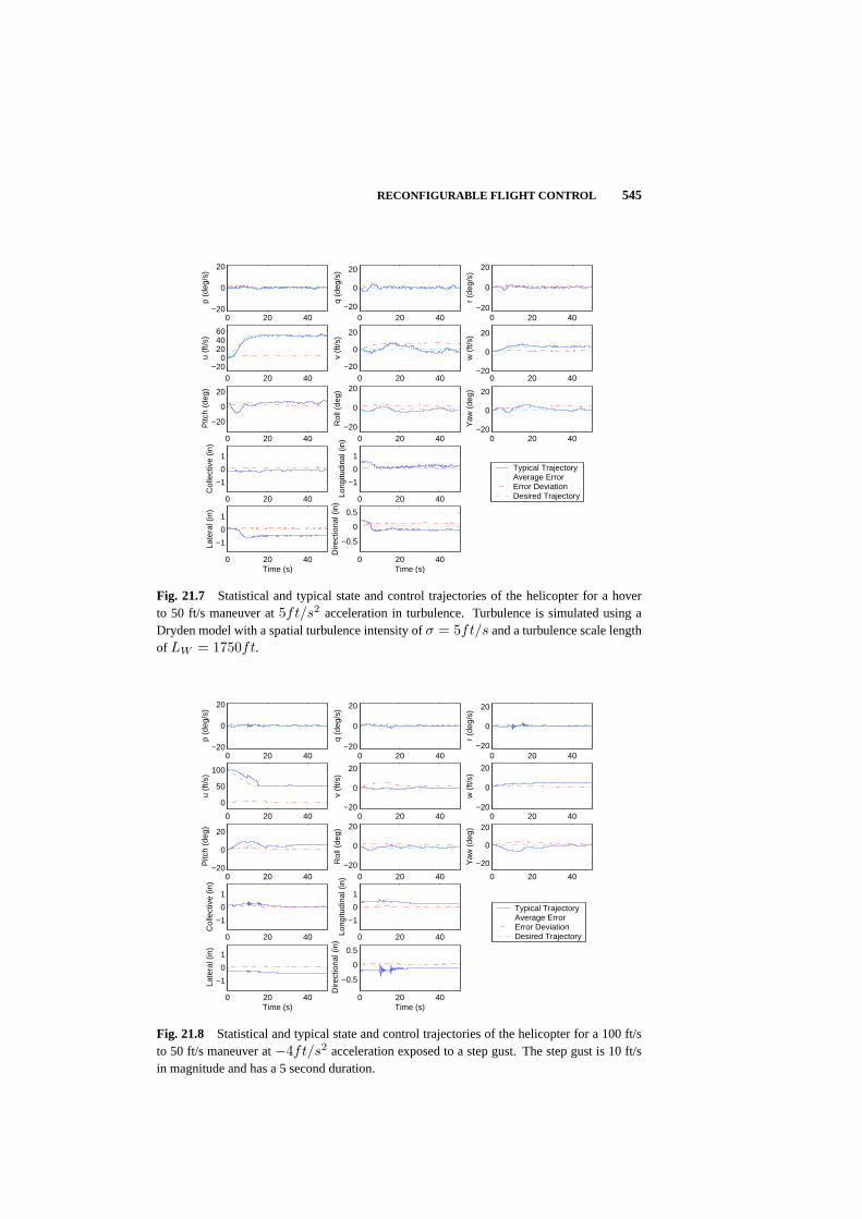
RECONFIGURABLE FLIGHT CONTROL 545
0 20 40−20
0
20
p (d
eg/s
)
0 20 40−20
0
20
q (d
eg/s
)
0 20 40−20
0
20
r (d
eg/s
)
0 20 40−20
0204060
u (f
t/s)
Typical TrajectoryAverage ErrorError DeviationDesired Trajectory
0 20 40−20
0
20v
(ft/s
)
0 20 40−20
0
20
w (
ft/s)
0 20 40
−20
0
20
Pitc
h (d
eg)
0 20 40−20
0
20
Rol
l (de
g)
0 20 40−20
0
20
Yaw
(de
g)
0 20 40
−1
0
1
Col
lect
ive
(in)
0 20 40
−1
0
1
Long
itudi
nal (
in)
0 20 40
−1
0
1
Time (s)
Late
ral (
in)
0 20 40
−0.5
0
0.5
Time (s)
Dire
ctio
nal (
in)
Fig. 21.7 Statistical and typical state and control trajectories of the helicopter for a hoverto 50 ft/s maneuver at5ft/s2 acceleration in turbulence. Turbulence is simulated using aDryden model with a spatial turbulence intensity ofσ = 5ft/s and a turbulence scale lengthof LW = 1750ft.
0 20 40−20
0
20
p (d
eg/s
)
0 20 40−20
0
20
q (d
eg/s
)
0 20 40−20
0
20
r (d
eg/s
)
0 20 40
0
50
100
u (f
t/s)
Typical TrajectoryAverage ErrorError DeviationDesired Trajectory
0 20 40−20
0
20
v (f
t/s)
0 20 40−20
0
20
w (
ft/s)
0 20 40−20
0
20
Pitc
h (d
eg)
0 20 40−20
0
20
Rol
l (de
g)
0 20 40
−20
0
20
Yaw
(de
g)
0 20 40
−1
0
1
Col
lect
ive
(in)
0 20 40
−1
0
1
Long
itudi
nal (
in)
0 20 40
−1
0
1
Time (s)
Late
ral (
in)
0 20 40
−0.5
0
0.5
Time (s)
Dire
ctio
nal (
in)
Fig. 21.8 Statistical and typical state and control trajectories of the helicopter for a 100 ft/sto 50 ft/s maneuver at−4ft/s2 acceleration exposed to a step gust. The step gust is 10 ft/sin magnitude and has a 5 second duration.
546 HELICOPTER FLIGHT CONTROL USING DIRECT NDP
redundancies. However, on any existing helicopter the loss of a main rotor actuatoris catastrophic. This section describes how direct NDP can be be used as a recon-figurable flight control method for helicopter actuator failures, and demonstrates themethod on a (rather benign) actuator failure.
Direct NDP already has been successfully demonstrated as a learning control schemefor helicopter flight control. From a neural control perspective this is a majoraccomplishment as it illustrates that neural networks can be taught to control verysophisticated unstable systems. It is now shown that direct NDP also has the capabilityto learn to control these sophisticated systems even when one of the underlyingcontrols fails. One implication is that direct NDP may be applicable to failureaccommodation for other physical systems where the failure accommodation solutionis not apparent using known underlying design principles.
To perform reconfigurable flight control, the direct NDP controller simply needs tobe trained to learn to recover from the failure in the same manner that it was trainedto control the aircraft in the prior sections. The control goal is to maintain the desiredaircraft states. If needed, weighting factors can be used in the reinforcement signalto place different emphasis on the various aircraft states. This allows certain lessimportant states to be sacrified while emphasis is placed on the more important aircraftstates. For example, the control goal may permit some variation in longitudinalvelocity, while maintaining emphasis on zero steady state angular rates (i.e. keep theaircraft upright).
The implementation of direct NDP for reconfigurable flight control can be identicalto that presented earlier. However, it was found that direct NDP performs muchbetter for reconfigurable flight control if one change is made. This change is tohave the direct NDP controller “control” blade angles, rather than actuator positionas shown in Figure 21.6. The performance of the new implementation is improvedbecause it minimizes the amount of terms required to be computed during back-propagation when training the controller (and eliminates the difficulty in computingone of the terms). However, in doing so, this adds one piece of expert knowledge,the mechanical relationship that exists between the actuators and the blade anglesin the upper flight control system (e.g. the swashplate and pitch links). While thisrelationship is well known, adding this “expert knowledge” does remove some of thepurity of direct NDP as a generic learning system.
The ability of direct NDP to learn to control the helicopter when a control actuatorfails is now demonstrated. Consider a helicopter flying at 60 knots that suffers amain rotor actuator failure at timet = 5.0s. Figure 21.9 shows the recovery from thefailure when using direct NDP, in contrast to a classically designed PID controllerwhich is unable to retain control of the helicopter.
Though the failure was more benign than what may be typically expected, in the sensethat the failure position was very close to the trim position, it does illustrate that directNDP is able to learn to accommodate such failure without any expert knowledge ofthe system. Such learning-based failure accommodation may have promise for failurerecovery in other systems where the dynamics are not well understood. However, itshould be mentioned that direct NDP for RFC does not find solutions for all failure
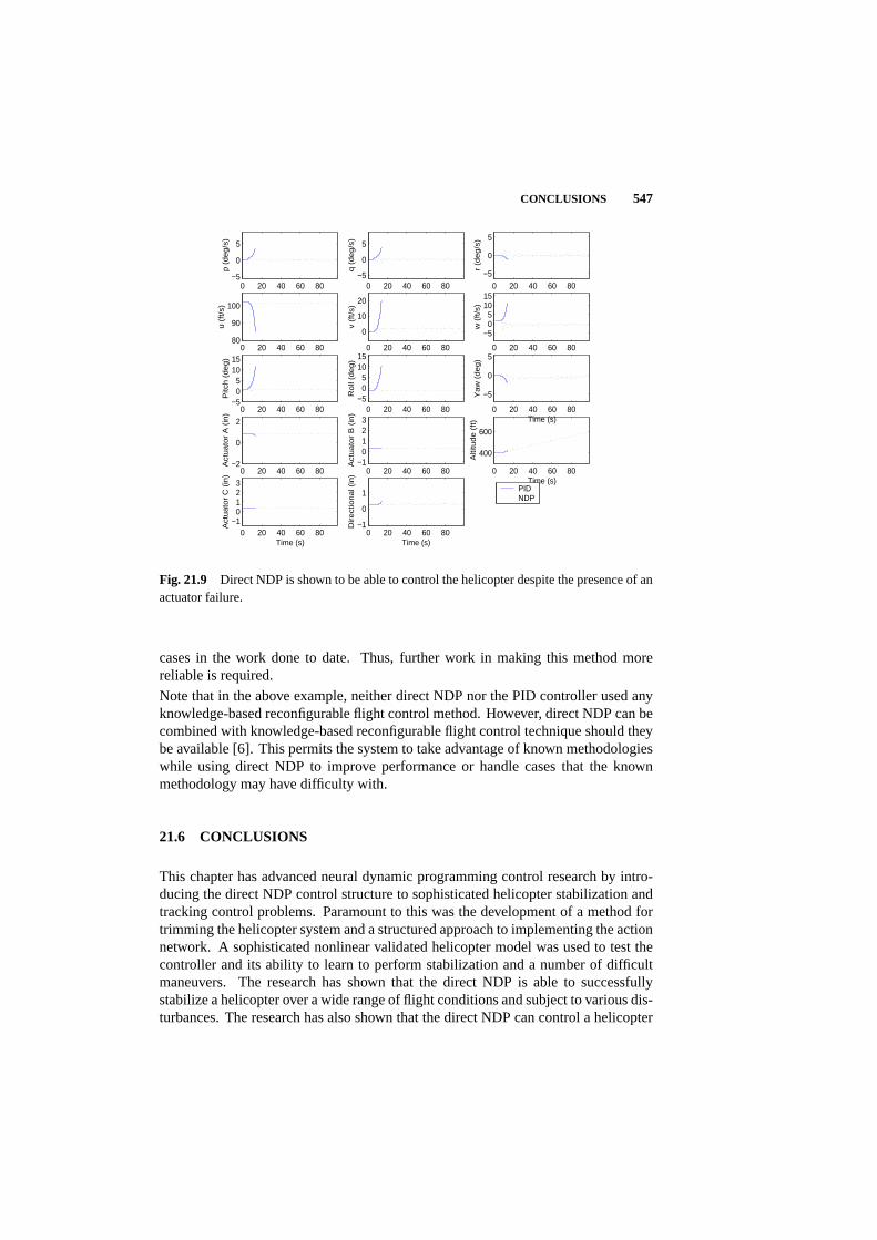
CONCLUSIONS 547
0 20 40 60 80
400
600
Time (s)A
ltitu
de
(ft)
0 20 40 60 80−5
0
5
p (
de
g/s
)
0 20 40 60 80−5
0
5
q (
de
g/s
)
0 20 40 60 80
−5
0
5
r (d
eg
/s)
0 20 40 60 8080
90
100
u (
ft/s
)
0 20 40 60 80
0
10
20
v (f
t/s)
0 20 40 60 80
−505
1015
w (
ft/s
)
0 20 40 60 80−5
05
1015
Pitc
h (
de
g)
0 20 40 60 80−5
05
1015
Ro
ll (d
eg
)
0 20 40 60 80
−5
0
5
Time (s)
Ya
w (
de
g)
0 20 40 60 80−2
0
2
Act
ua
tor
A (
in)
0 20 40 60 80−1
0123
Act
ua
tor
B (
in)
0 20 40 60 80−1
0123
Time (s)
Act
ua
tor
C (
in)
0 20 40 60 80−1
0
1
Time (s)
Dire
ctio
na
l (in
)
PIDNDP
Fig. 21.9 Direct NDP is shown to be able to control the helicopter despite the presence of anactuator failure.
cases in the work done to date. Thus, further work in making this method morereliable is required.
Note that in the above example, neither direct NDP nor the PID controller used anyknowledge-based reconfigurable flight control method. However, direct NDP can becombined with knowledge-based reconfigurable flight control technique should theybe available [6]. This permits the system to take advantage of known methodologieswhile using direct NDP to improve performance or handle cases that the knownmethodology may have difficulty with.
21.6 CONCLUSIONS
This chapter has advanced neural dynamic programming control research by intro-ducing the direct NDP control structure to sophisticated helicopter stabilization andtracking control problems. Paramount to this was the development of a method fortrimming the helicopter system and a structured approach to implementing the actionnetwork. A sophisticated nonlinear validated helicopter model was used to test thecontroller and its ability to learn to perform stabilization and a number of difficultmaneuvers. The research has shown that the direct NDP is able to successfullystabilize a helicopter over a wide range of flight conditions and subject to various dis-turbances. The research has also shown that the direct NDP can control a helicopter

548 HELICOPTER FLIGHT CONTROL USING DIRECT NDP
for a wide range of realistic maneuvers and over a wide range of flight conditions,a few examples of which were illustrated. Thus, it appears that direct NDP is aviable candidate for controlling complex MIMO systems and is suited particularlywell for on-line and complex multi-axes coupling control applications. The resultshave demonstrated the generalization capability of a learning control system, namelydirect NDP, to a large, continuous state problem. The same principles can also bedirectly applied to large, discrete state/action problems.
This chapter has presented a general overview of a complex design using direct NDP.The emphasis has been on the procedure of formulating the problem, setting upthe objectives, implementation details, results and insights that can be gained fromdoing direct NDP designs. More detailed examinations of the helicopter problemincluding the helicopter model, the trim system, flight control system requirements,helicopter geometry and optimization for reconfiguration consideration, and manyother technical details can be found in [7], or [4, 5, 6] for helicopter stabilization,tracking, and reconfiguration control, respectively.
Acknowledgments
The research was supported by the National Science Foundation under grants ECS-0002098and ECS-0233529. The first author was also supported by an academic leave provided by theBoeing Company.
Bibliography
1. S. Balakrishnan, and V. Biega, “Adaptive-critic-based neural networks for aircraftoptimal control,”AIAA Journal of Guidance, Control, and Dynamics,vol. 19,no. 4, pp. 731-739, 1996.
2. J. A. Bagnell, and J. Schneider, “Autonomous helicopter control using rein-forcement learning policy search methods,”Proceedings of the InternationalConference on Robotics and Automation,vol. 2, pp. 1615-1620, 2001.
3. G. Buskey, J. M. Roberts, and G. Wyeth, “Online learning of autonomous heli-copter control,”Australasian Conference on Robotics and Automation,pp. 19-24,2002.
4. R. Enns, and J. Si, “Apache helicopter stabilization using neural dynamic pro-gramming,”AIAA Journal of Guidance, Control, and Dynamics,vol. 25, no. 1,pp. 19-25, 2002.
5. R. Enns, and J. Si, “Helicopter trimming and tracking control using direct neuraldynamic programming,”IEEE Transactions on Neural Networks,vol. 14, no. 4,pp. 929-939, 2003.
6. R. Enns, and J. Si, “Helicopter flight-control reconfiguration for main rotoractuator failures,”AIAA Journal of Guidance, Control, and Dynamics,vol. 26,no. 4, pp. 572-584, 2003.
7. R. Enns,Neural dynamic programming applied to rotorcraft flight contorl andreconfiguration,Ph.D. Dissertation, Arizona State University, 2001.
8. S. Kumar, J. Harding, and S. Bass, “AH-64 apache engineering simulationnon-real time validation manual,”Technical Report USAAVSCOM-TR-90-A-010,1990.
9. D. Prokhorov, and D. Wunsch II, “Adaptive critic designs,”IEEE Transactionson Neural Networks,vol. 8, no. 5, pp. 997-1007, 1997.
10. H. Shim, T. J. Koo, F. Hoffmann, and S. Sastry, “A comprehensive study ofcontrol design for an autonomous helicopter,”Proceedings of the 37th IEEEConference on Decision and Control,vol. 4 , pp. 3653-3658, 1998.
549

550 BIBLIOGRAPHY
11. J. Si, and J. Wang, “On-line learning by association and reinforcement,”IEEETransactions on Neural Networks,vol. 12, no. 2, pp. 264-276, 2001.
12. E. A. Wan, A. A. Bogdanov, R. Kieburtz, A. Baptista, M. Carlsson, Y. Zhang,and M. Zulauf, “Model predictive neural control for aggressive helicopter ma-neuvers,”Software Enabled Control: Information Technologies for DynamicalSystems,IEEE Press, 2003.
22 Towards Dynamic StochasticOptimal Power Flow
JAMES A. MOMOH
National Science Foundation
Editor’s Summary: This chapter deals with optimal power flow tools, whichmust be capable of handling multiple objectives while simultaneously satisfyingoperational constraints. This chapter contains an overview of the generalized optimalpower flow problem, description of the traditional techniques used for optimal powerflow and their limitations, and discussion of the current state-of-the-art in robustoptimal power flow. Finally, the author presents a generic framework for fittingADP techniques into the optimal power flow framework. This is presented as anopen problem for ADP and the framework is given so that researchers can test andcompare different techniques.
22.1 GRAND OVERVIEW OF THE PLAN FOR THE FUTURE OPTIMALPOWER FLOW (OPF)
Optimal Power Flow (OPF) is one of the most important operational functions ofthe modern day energy management system. There are several objectives of optimalpower flow and among them are: finding the optimum generation amongst theexisting generating units, such that the total generation cost is minimized, whilesimultaneuously minimizing the voltage deviation of the system to improve thesecurity and loss minimization of the entire network and furthermore attempting tosatisfy the power balance equations and various other constraints in the system. Theconstraints imposed on the system include voltage magnitudes of the buses and activeand reactive power constraints as well as transformer or phase shifter taps constraints,which are discrete in nature. The optimal power flow tool must be capable of handlingmultiple objectives while simultaneously satisfying operational constraints.
A power flow may have any number of operating limit violations. When such condi-tions occur, the operator may wish to determine if the troubles can be alleviated byappropriate corrective actions. This analytical process is known as Optimal Power
551

552 TOWARDS DYNAMIC STOCHASTIC OPTIMAL POWER FLOW
Flow. The optimal actions analyses are formulated as an optimization problemwith the objective of minimizing load curtailment, MW generation redispatched, andtransformer phase angle adjustment. It includes a standard ac power flow solutionwith local automatic adjustments, power system network linearization, and a linearprogramming solution to relieve the overload and voltage limit violations. The cor-rective action algorithm must recognize several types of constraints and controls.Constraints are operating limits imposed on bus voltages, branch flows, and powertransfers over interfaces, etc. The system troubles in contingency analysis are vio-lations of such operating constraints. Controls include generator real and reactivepower generation, phase shifter angles, and busload curtailment schedule voltages ofgenerators and ULTC-transformers, reference values of HVDC systems and Flexi-ble AC Transmission System devices (Unified Power Flow Controller UPFC, StaticVAR Compensators SVC, Solid State Synchronous Compensator STATCOM, andThyristor Controlled Series Capacitor (TCSC).
The objective of the corrective action algorithm is to observe all constraints whileoptimizing the weighted sum of the control movement. The priorities of controlactions are phase shifter control followed by generator real power shifts, and ifrequired, load curtailment. This priority order is maintained by assigning the highervalue of weight to the lower priority controls. There are several approaches adopted inthe analytical process, which involves the application of intelligent systems, heuristicmethods and hybridized methods incorporating both heuristic and computationalintelligence techniques.
Optimal power flows have been widely used in planning and real-time operation ofpower systems for active and reactive power dispatch to minimize generation costsand system losses and to improve system voltage profiles. Typically, problems ofvoltage constraints and stability issues have been assumed decoupled and thus treatedindependently. However, as the system operates closer to its stability limits, such asits voltage collapse point, due to market pressures, this assumption does not applyany longer, and hence there is a need to consider these limits within the OPF. Byincluding these stability limits in the OPF problem, optimization procedures can alsobe used to improve the overall system security while accounting at the same time forthe costs associated with it, which is becoming an important issue in open electricitymarkets. The voltage stability problem in power systems has been widely studied,and the basic mechanisms that lead to a network voltage collapse have been identifiedand are now clearly understood. It has been demonstrated that the overall stability ofthe system is closely associated with the proximity of a system to a voltage collapsecondition, i.e., as the system approaches a voltage collapse point, its stability regionbecomes smaller, resulting in a system that is less likely to survive contingencieshence, as a first approximation, one can use voltage stability criteria to account forthe overall system stability.
Some current research includes neural network optimal power flow when seen in itsentirety is probably the case that the operation and control of an interconnected powersystem is the largest and most involved control problem of any kind in any field. Asusual, the cost side of the optimization problem so formulated is revenue generation,
GRAND OVERVIEW OF THE PLAN FOR THE FUTURE OPF 553
which are amongst the largest of any single body or organization of unified structureand on the supply side is the life-blood of every modern and developed economy.
In common with current usage, the on-line computer-based facilities on which systemoperation, control and management now draw so extensively are referred to as EnergyManagement Systems (EMS’s). Modern EMS’s provide extensive on-line computer-based control and communication facilities for meeting the central requirement inelectricity supply of achieving the greatest possible system utilization at the lowestpossible running costs subject to very many constraints both technical and non-technical.
The optimal power flow function is a key one in the suite of software modules thatmake up an EMS. At the present time, the on-line control and management facilitiesthat OPF can achieve are limited by the processing capabilities of the computersystem that supports it. Because OPF is one of the most involved and extensive ofall EMS functions, its computing system overheads are high.
With the current research and state-of-the-art technology in OPF tools, there arepertinent issues that have not been adequately tackled. The traditional OPF involvesthe determination of the instantaneous optimal steady state solution of the power gridwithout addressing the need for time dependency and to some extent handling ofdiscrete as well as continuous parameters of the system components. The drawbacksare:
• Lack of Foresight: the capability of the existing OPF to predict the future interms of asset valuation and economic rate of return on investment in powersystem infrastructure subject to various system dynamics and network con-straints.
• Lack of explicit optimization technique to handle perturbation and noise.
Since foresight is critical to the power system as far as network expansion, right ofway procurement for transmission corridors and overall rate of return on investmentare concerned, new tools are needed for the operation of the deregulated power systemmarkets.
With these features fully integrated into traditional OPF, the deregulated power systemmarkets can fully deal with both foresight and stochastic dynamics of the optimalpower flow problems of utility companies worldwide.
New OPF tools capable of handling the traditional OPF problems such as UnitCommitment, Economic dispatch, loss minimization, VAR Planning, congestionmanagement through the evaluation of Available Transfer Capability, market designsand price caps as well as voltage stability problems are needed. The tools must havein addition to handling the traditional OPF problems, a futuristic and time dependencemodule for evaluation of the impact of investment for the future while taking intoaccount the stochastic nature of the power system network. These will thereforerequire new models of the existing system to be developed and incorporated into thenew OPF.

554 TOWARDS DYNAMIC STOCHASTIC OPTIMAL POWER FLOW
22.1.1 Achievements of OPF and Documented Limitations
From the general class of OPF problems solved to date and the methodologiesemployed, there are significant achievements worthy of mention. Among them are:
Optimal power flow using successive sparse and non-sparse quadratic programming,successive non-sparse separable programming, Newton’s method and most recentlyInterior point methods. Some of these implementation techniques wit appropriatemodeling and formulation of the OPF problem resulted in commercial software pro-grams. These programs are being maintained regularly to achieve high performanceand give better, accurate results compared to their earlier versions due to improve-ments made in the optimization theories and significant research advances over theyears. These improvements include high flexibility and modeling of new objec-tive functions and constraints, reliability of solutions obtained, good user friendlyinterface and visualizations.
Research has led to the development of an ultra-high-speed computing architecturewith the aim of allowing all aspects of OPF to be implemented. The architecture isone based on the massively parallel-processing structure of arrays of neural networks.The main features of OPF in EMS are:
• Operating cost minimization.
• Network active-power loss minimization and restoration control strategies.
• Control of generator active-power loading levels, off-nominal tap-positionsof transformers, target voltage settings of on-load tap-changing transformers,generator excitation controllers, and static VAR compensators, selection forservice of fixed-value reactors and capacitors used for reactive-power andvoltage control purposes
• Inclusion of contingency constraints relating to any number of postulated out-age conditions and power network configurations
• Post-contingency rescheduling so that optimal operation is achieved withoutviolating any security constraint
• Ultra-high-speed computation in which the computing time is independent ofsize of the power network and the number of postulated contingency cases ofwhich it is required to take account.
• Bidding analysis and strategizing of competitive bidding
• Market oriented dispatch and demand side bidding
• Bidding and contracting rules formulation
• Ancillary services/reactive VAR support
• Load curtailment analysis and post-optimal analysis.
• Dispute resolution and litigation

GRAND OVERVIEW OF THE PLAN FOR THE FUTURE OPF 555
22.1.1.1 Some Extended Application of OPF
• Capacitor Installation
Optimal sizing and location of new capacitors in the network to ensure a definedlevel of steady-state security. This is solved as Security Constrained OptimalPower Flow to minimize the investment and operating costs. The currentchallenge is to embed this OPF solution in a multi-year planning process thatconsiders variation in system load, generation and network topology changes.
• Transmission Service Pricing
Transmission constrained marginal costs can be obtained for factors includingbinding power system operating constraints, production capacities, equipmentregulation limits, area interchanges, losses and bus powers. The cost of MVArsupply and delivery is being addressed by utilities in the deregulated powerindustry.
Through the use of OPF in EMS, utilities tend to benefit in system managementand control in achieving the greatest possible network system utilization at thelowest possible operating costs.
22.1.1.2 Challenges and Limitations to On-Line OPF ImplementationThere are numerous challenges faced in implementing OPF in the deregulated powersystem, including the following specific operational requirements and challenges.
One of the operational requirements is robustness. OPF solutions should not besensitive to the starting point used, and changes in solution point should be consistentwith that in the operating constraints.
The three main problems faced are: the existence of multiple local, weak or non-convergence of the solution method used, poor input data and inadequate models ofthe power system to be able to solve real life problems. For local minima problem,the nature of actual power system is responsible for getting the solution stacked.However proper models and operating information is needed to fully specify theproblem and eliminate the non-uniqueness. The convergence problem arises as aresult of an inherent limitation of the methodology employed for the solution andhence more serious. This calls for new methods and tools from other fields of researchto address such limitations.
Accurate data to mimic the existing power system must be modeled and fine tunedto meet the network standards and operating constraints before attempting to run theprogram. Choice of initial starting point of the solution algorithm is necessary toavoid entrapment in local extrema instead of global extrema of the operating regimeof the power system network.
In the new deregulated power system, the capabilities of conventional optimal powerflow program itemized above must be enhanced to handle new components, discreteand continuous parameters and accurate modeling of system components as well asextensive data involving many power systems interconnections. There is the need forexpansion of the scope of OPF problem to embrace:

556 TOWARDS DYNAMIC STOCHASTIC OPTIMAL POWER FLOW
• More flexible controls and constraint priority strategies,
• Incorporation of control and load dynamics,
• Inclusion of start-up and shut-down constraints of certain controls and otheroperating constraints that meet specific practical requirements,
• Hydro modeling,
• Incorporating voltage stability and other dynamic constraints relevant in theon-line environment,
• Modeling of non-linear and voltage dependent loads,
• Coordination of controls with different response characteristics,
• Modeling of prohibited operating zones on the cost curves,
• Effective modeling of external system suitable for optimization applications,
• Time restrictions on control constraint violations,
• Cost penalty thresholds for constraints reinforcements,
• Effective branch switching modeling.
Conventional and existing OPF tools use all possible control actions for getting theoptimal solution, but it may not be feasible to execute more than a limited number ofcontrol actions. The remedies could be (1) to limit number of control action of eachtype (2) assign initiation cost for each control action (3) utilize fuzzy based methodto reduce ineffective controls, though further work is needed in this area to lead torobust solutions and (4) compromise in the short run by reliance on near-optimalsolutions that incorporate sound engineering rules.
For modeling discrete quantities of the power system, the step-size of the discretevariables should be sufficiently small to warrant continuous approximations. Thepossible approaches for accurate results and modeling of discrete variables are:
• Simulations of conventional power flow program with all discrete variablesfixed on their steps.
• Introduction of penalty function for discrete controls
• Implementing a trajectory of OPF control shifts that does not exacerbate exist-ing violations or cause additional ones.
Consistency of OPF with other online functions is vital to the overall benefit ofthe system. This required consistency in the study mode and research as well asclosed loop implementation of OPF is a current subject of research. The design ofinterface and of OPF in closed-loop mode with other functions viz. Unit Commitment,Economic Dispatch, Security analysis, and Automatic Generation Control AGCpresents formidable tasks. The central aspect is the effective coordination of OPF-ED-AGC control hierarchy.
GENERALIZED FORMULATION OF THE OPF PROBLEM 557
22.2 GENERALIZED FORMULATION OF THE OPF PROBLEM
Minimize F (x, u)
subject tog(x, u) = 0 Equality constraintsh(x, u) ≤ 0 Inequality constraints
Wherex′s are the state variables of the power system andu′s are the control param-eters of the power system.
A. Objective Function Definition
1. Minimum fuel costThe cost function of the generators is assumed to be quadratic and the objectivefunction can be stated as:
Minimize F =NG∑
i=1
(aiP2gi+biPgi + ci) (22.1)
where
Pgi : Real power output of theith generator;
ai, bi andci : Cost coefficients of theith generator;
NG : Total number of generator in the system;
2. Minimum line flow overloadsThe objective function for minimal line overload on the transmission system is:
Minimize F =NL∑
i=1
(Pij(t)− Pmax
ij (t))2
(22.2)
Where
Pij(t) : Real power flow through theijth transmission line at time staget;
Pmaxij (t) : Maximum power flow through theijth transmission line at time
staget;NL : Total number of overloaded lines.
3. Minimum transmission lossesThe losses in a power system are directly related to the slack bus power. The optimalpower flow model for loss minimization problem in a typical power system is:
Minimize FL = F(Pslack) (22.3)

558 TOWARDS DYNAMIC STOCHASTIC OPTIMAL POWER FLOW
Where
Pslack : Power at the swing or reference bus;
FL : System Loss function;
Pslack : Active power being delivered at the slack bus, and it is a function of
the system state variables such thatPslack = Fslack(V, θ, T).
4. Minimal adjustment of phase shiftersHere we seek to minimize the number of phase shifters that are adjusted in a givetime frame such that the objective function is:
Minimize F =NS∑
i=1
Wiφi (22.4)
where
Wi : Weighting factor of the phase shifter;
φi : Phase shift angle of theith phase shifter;
NS : Total number of phase shifters in the network.
5: Minimal generation impactThe least generation shift is desired for the control action that is taken to relieve orreduce the power system congestion. The mathematical formulation of the objectivefunction is stated as:
Minimize F =NG∑
i=1
(Pgi(t)− P o
gi(t))2
(22.5)
where
P ogi(t) : Real power output of theith generator before installing the phase shifter
at time staget;
φi : Actual real power output of theith generator after installing the phase
shifter at time staget;
NG : Total number of overloaded lines.
B. Constraints Modeling in Optimal Power FlowIn addition to the general linear/nonlinear constraints, the constraints relating to phaseshifter variables such as phase shifter angle and maximal adjustment numbers shouldbe included in the OPF formulation with phase shifter. It is important to selectsuitable constraints for OPF with phase shifter and the candidate constraints are asfollows:
GENERALIZED FORMULATION OF THE OPF PROBLEM 559
1. Upper/Lower limits of real power output of generators
Pmingi ≤ Pgi ≤ Pmax
gi (22.6)
where
Pgi : Active power of generatori;
Pmingi , Pmax
gi : Lower and upper real generation limits of uniti, respectively.
2. Power balance equation
NG∑
i=1
Pg i =ND∑
k=1
Pd k + PL (22.7)
where
Pgi : Active power of generatori;
Pdk : Active power at load busk;
PL : Total system losses;
NG : Total number of generator buses in the network;
ND : Total number of load buses in the network.
3. Upper/Lower limits of reactive power output of generator
Qmingi ≤ Qgi ≤ Qmax
gi (22.8)
where
Qgi : Reactive power of generatori;
Qmingi , Qmax
gi : Lower & upper reactive generation limits of uniti, respectively.
4. Upper/Lower limits of node voltage at PV buses
V mingi ≤ Vgi ≤ V max
gi (22.9)
where
Vgi : Node voltage of generatori;
V mingi , V max
gi : Lower and upper voltage limits of generator busi, respectively.
5. Upper/Lower limits of node voltage at PQ buses
V mindi ≤ Vdi ≤ V max
di (22.10)
560 TOWARDS DYNAMIC STOCHASTIC OPTIMAL POWER FLOW
where
Vgi : Node voltage at load busi;
V mindi , V max
di : Lower and upper limits of the node voltage at load busi.
6. Power flow constraints of transmission lines
Pminij ≤ Pij ≤ Pmax
ij (22.11)
where
Pij : Active power flow through lineLij ;
Pminij , Pmax
ij : Lower and upper power limits of lineLij .
7. Upper/Lower limits of transfer capacity of the network[V 2
i + V 2j − 2ViVj cos(θ i − θ j)
]/ZL(l)2I2
L max(l) ≤ 0 (22.12)
where
Vi : Voltage magnitude at busi;
Vj : Voltage magnitude at busj;
IL : Thermal or current limit of line,Lij ;
ZL : Impedance of transmission line,Lij .
8. Upper/Lower transformers limits (ULTCs)
Tmini ≤ Ti ≤ Tmax
i , i ∈ NT (22.13)
where
Ti : Tap setting of transformeri;
Tmini , Tmax
i : Lower and upper tap limits of transformeri,
respectively.
9. Step length of phase shift angle
φmini ≤ φi ≤ φmax
i ∀ i ∈ 1, NPS (22.14)
where
φi : Phase angle of theith transformer;
NPS : Total number of phase shifters in the network.
GENERAL OPTIMIZATION TECHNIQUES USED IN SOLVING THE OPF PROBLEM 561
10. The maximal adjustment times of phase shifter per day
Nsch∑
i=1
φmini ≤
Nsch∑
i=1
φi(t) ≤Nsch∑
i=1
φmaxi (22.15)
where
φi(t) : Angle of phase shifter transformeri at timet;
φmaxi : Upper phase angle limit of theith phase shifter;
φmini : Lower phase angle limit of theith phase shifter;
Nsch : Set of scheduled phase shifter transformers.
For the above-mentioned constraint set, it is necessary to analyze whether all theseconstraints are active or suitable for optimal power flow calculations with phase
22.3 GENERAL OPTIMIZATION TECHNIQUES USED IN SOLVINGTHE OPF PROBLEM
Various optimization methods are utilized in the solution of the general OPF problemwith multiple objectives and with equality and inequality constraints. These methodsinclude:
• Linear programming
• Nonlinear programming
• Quadratic programming
• Interior point (including Dual Affine algorithm, Primal Affine algorithm andBarrier algorithm)
• Hybridized method incorporating any of the conventional approaches and com-putational intelligence method.
• Computational intelligence techniques including evolutionary programming,artificial neural networks and adaptive critics networks.
These methods are suitable for the evaluation of the generalized optimal power flowproblem. Each is suitable in its own domain with peculiar strengths and weakness.Based on the level of accuracy, faster convergence and storage required any of themethods could be used for the requirements needed.
In the evaluation of multi-objective functions coupled with both equality and inequal-ity constraints analytical hierarchical process and pareto-optimal analysis could beused in conjunction with any of the above methods to assign priority and ranking to

562 TOWARDS DYNAMIC STOCHASTIC OPTIMAL POWER FLOW
controls options used in the general formulation of the Optimal Power Flow problem.
Description of Optimization TechniquesOptimization techniques are characterized by the efficiency of the techniques em-ployed for obtaining a ’good’ starting or initial point, the robustness and completenessof the iterative process, and the termination conditions. Many approaches currentlyexist for solving the optimization problems in power system such as unit commit-ment, resource allocation, economic dispatch or generation rescheduling, networkreconfiguration, and load shedding. These optimization approaches, some of whichhave been reviewed earlier, are characterized by the certain attributes/criteria that areused to evaluate optimal power flow tools. These attributes and criteria for evaluationinclude:
Adaptability
This is an evaluation measure of the capability to add new constraints, limits,and optimization function, which remain solvable by the optimization tech-nique that is used in the optimal power flow tool.
Practicality
This involves evaluation of the method’s ability to handle practical systemsas well as physical system constraints. Further, it involves the ability of themethod to display or convey the correct answers constantly to the user underdifferent system conditions and inputs.
Efficiency / Reliability
This involves the method’s ability to compute and convey the correct solutionto the optimization problem in a minimum or reasonable time.
Sensitivity
This involves the measure of the method’s reaction to practical changes suchas the effect of parameter or network changes in the system. The sensitivity ofthe optimization method can be a useful attribute for quickly computing globaloptimal solution in an environment where computational time is costly.
A brief review and evaluation of the mathematical programming methods commonlyused in optimal power flow is discussed below.
22.3.1 Linear Programming (LP)
Linear Programming, introduced by G.B. Dantzig (1947), exploits the linear structureof many problems in a wide variety of applications, including power system operationand planning. Typically, Linear Programming utilizes two method of computation.They are 1) the Simplex Method and 2) the Revised Simplex Method. The revisedsimplex method is more commonly used in practical applications. Variants of Interior
GENERAL OPTIMIZATION TECHNIQUES USED IN SOLVING THE OPF PROBLEM 563
Point methods are also used for Linear Programming problems and several OPF toolsexist using LP formulations.
There exist several solution techniques for solving the optimal power flow problemthat are based on linear programming models. The objective function in the OPFproblem is approximated to a linear relationship relative to the state and controlvariables. A first order Taylor series approximation is used which assumes continuityand convexity of the objective function.
Linear Programming has been used extensively to solve real and reactive generationcosts in OPF as well as transmission loss calculations. The method, typically therevised simplex technique, assumes a linear model of the problem, which introducessome degree of inaccuracy in the final results. Its ability to handle discrete controlsis done using several variants of Integer programming such as the branch and boundmethod.
22.3.2 Nonlinear Programming
In power system applications and analysis, the Newtonian method in nonlinear pro-gramming is among the most popular approaches. Other techniques in classicaloptimization include Quadratic Programming (QP), Lagrangian Multiplier and Re-duced Gradient Methods. These methods are applicable to solving typical optimalpower flow problems of electric power system. This is because most problems can besufficiently modeled as piece-wise nonlinear functions suitable for the power systemwhich is inherently nonlinear.
Nonlinear Programming (NLP) typically employs Lagrangian or Newtonian Tech-niques for the constrained and unconstrained optimization problems. The approachassumes that all objective functions are modeled as smooth and continuous functions.However, the mathematical response of the power system diverts from this assump-tion in many instances. Static devices such as the phase shifter transformers, seriesand shunt components (Capacitor and Inductor banks), Flexible AC TransmissionDevices (FACTs), and Under Load Tap Changers (ULTCs) are devices with discretetransfer and control functions. Thus, nonlinear programming methods often suffer ifthe approximations to the actual models for these devices are not sufficiently accurate.Theλ lambda parameter utilized in this approach does not reflect the future of thepower system and therefore lacks foresight. Integrating foresight or dynamics andstochasticity into this approach will ensure the correct response and behavior of thepower system in the future and can help in power system planning.
In power system applications, the Newtonian method takes advantage of the convexityand continuity conditions of the load flow model and is used in many powerfuloptimization tools where solution accuracy of AC power flow calculations is to bepreserved. The commonly used Newton, Gradient Search, and MINOS optimizationpackages are available in the form of commercial-grade programs for solving thegeneral optimal power flow problems.

564 TOWARDS DYNAMIC STOCHASTIC OPTIMAL POWER FLOW
22.3.3 Interior Point Method
Interior Point methods represent a special case for solving optimization problemsusing the linear programming model. The basic approach was developed and bench-marked by Karmakar et. al. 1986. This has led to many variants of the approach,which can be adapted to many common real-time problems. These variants includethe Primal Affine method, the Dual Affine method, and the Projection or the Kar-makar’s technique and anextendedInterior Point algorithm that was developed atHoward University.
The projection scaling method or Karmakar’s algorithm is characterized by it abilityto converge with any feasible initial point. This makes the method attractive andpowerful for engineers and software developers. But the method depends on thelocation of a good initial point inside the polytope or region that is bounded by theconstraint set of the optimization problem. Increasing the dimension of the problemdoes not degrade the computational speed of the algorithm.
The primal affine method is faster than the projection scaling method. It is a specialcase of the projection scaling method with improved computation of the step lengthof the translation vectors in the search space. The method solves linear objectivefunction subject to linearequalityconstraints.
The dual affine method is the fastest of the three commonly used variants of InteriorPoint being reviewed in this report. Similar to the primal affine method, it is an en-hanced version of the Karmakar’s scaling algorithm. The method utilizes a “barrier”or Logarithmic approach in computing the step lengths of the scaling vectors. Thismethod is applicable to optimization problems where the objective function is linearsubject to linear inequality constraints. A logarithmic penalty function is used in theformulation of the Lagrange function of the constrained optimization problem. Themethod employs minimal inverse calculations to increase the speed of computation.
Finally, in the past decade, primal-dual algorithms have emerged as the most impor-tant and useful algorithms from the interior-point class. Primal-dual algorithms,which include path-following algorithms (short-step, long-step, and predictor -corrector), potential-reduction algorithms, and infeasible-interior-point algorithms,can be extended to more general classes of problems such as semi-definite program-ming, and general problems in convex programming.
22.3.4 Barrier Optimization Method
The Barrier approach to a constrained optimization problem is the process of applyinga logarithmic or concave function as a shadow price or special purpose Lagrangianmultiplier. This process has let to an improvement in the solution of the Karush-Kuhn-Tucker (KKT) conditions of a linear programming problem. The method ofbounding the interior of the solution space, which is also used to analyze the efficiencyof the conjugate-gradient method in solving a system of linear equations, can also bealso extended to the interior point method. The relationships between the primal-dualNewton interior-point method and the logarithmic barrier function method has led to

THE QUADRATIC INTERIOR POINT (QUIP) METHOD 565
more robust optimization algorithms in this class that are less prone to infeasibilityunless the problem is ill-conditioned.
A special relationship between the primal-dual Newton interior-point method and thelogarithmic barrier function method has also led to solution of LP problems with aprimal-dual Logarithmic Barrier method. The solution method is based on solvingthe primal-dual penalty-barrier equations for a sequence of decreasing values of thescalar penalty-barrier parameter. An augmented penalty-barrier function is used asan objective function for both the primal and dual variables.
22.4 STATE-OF-THE-ART TECHNOLOGY IN OPF PROGRAMS: THEQUADRATIC INTERIOR POINT (QUIP) METHOD
The linear programming model that incorporates linear objectives and constraintsis often not suitable for adequate results to an OPF problem. As such, withoutcompromising the speed advantage of the projection of scaling methods of interiorpoint, a Quadratic Interior Point (QUIP) method has been developed.
In the QUIP formulation used for in power system applications, the objective functionif quadratic and the constraints set of the network and the devices on the powersystem have been linearized. The Quadratic Interior Point technique is by far thefastest of the variants of the interior point methods. Also, it is better at convergingto an acceptable solution giving a wide range of initial point solutions. The QUIPtechnique is the backbone of the computational tool, Robust Interior point OptimalPower Flow (EPRI/Howard University) under contract No. 3788-01. The researchthrust therein is aimed at extending its capability to handle discrete variable such asphase shifter.
The QUIP method is used in the state of the are in Optimal Power Flow Problems.In the previous section, we provided an analytical formulation and modeling of theOPF-based phase shifter problem. The solution strategy involves decomposing theproblem into a multi-stage procedure. The first stage involves solving the optimalpower flow problem using the QUIP method. This method is incorporated in theRobust Interior Point Optimal Power Flow Program (RIOPF) and is used to obtain theoptimal operating points without phase shifters. The second stage of the optimizationprocess involves application of the rule-base scheme to optimize the discrete phaseshifter tap setting in order to solve the line overload problem. The result of the OPFcalculations serves as input to the rule base system. The firings of the rules weredone to compute the discrete phase shifter tap setting under faulted or contingentscenarios.
Next, perform Cost-Benefit Analysis on the selected control strategies. It provides aneconomic rationale for using phase shifter control. Finally, the overall implementa-tion strategy contains a post-optimal analysis for shadow price calculation in order todetermine the impact of the phase shifters on the system. The final recommendationsfor phase shifter tap settings for optimal overload relief is now based on technical as
566 TOWARDS DYNAMIC STOCHASTIC OPTIMAL POWER FLOW
well as economic judgments.
The Interior Point Algorithm
The above-mentioned OPF model with phase shifter is a nonlinear mathematicalprogramming problem. It can be reduced by an elimination procedure. The reductionof the OPF model is based on the linearized load flow around base load flow solutionfor small perturbation. The reduced OPF model has the format:
Min F =12XT QX + GT X + C (22.16)
Subject toAX = B, with X ≥ 0 (22.17)
The model given in Eq. 22.16 - 22.17 has a quadratic objective function subject to thelinear constraints that satisfy the basic requirements of quadratic interior point (QIP)scheme. Generally, the effectiveness of interior point methods depends on a goodstarting point. The extended quadratic interior point (EQIP) method with improvedinitial conditions is presented in this paper. It features the improved starting pointand faster convergence.
Integrated OPF Design with IP Application
This section describes the overall optimal power flow design scheme that incorporatesthe phase shifter control. The scheme features an interior point-based optimal powerflow model and a rule-based scheme that is used to calculate the optimal adjustmentschemes of the phase shifter tap settings, limit checking of constraints, line overload-ing state checking, sensitivity analysis for ranking phase shifters, rule-based systemto handshake the adjustment of phase shifters, and a CBA and Shadow Price module.
22.5 STRATEGY FOR FUTURE OPF DEVELOPMENT
New extensions of RIOPF are needed for enhanced performance and improved ca-pability for general-purpose OPF problems embodying formulation of new powersystem constraints and the introduction of new power system components such asDistributed Generation resources and FACTS device technology. This new exten-sions should be able to handle the optimal location and sizing of DG’s and othersystem components
The RIOPF is a special purpose OPF tool that can be extended to integrate computa-tional intelligence techniques for enhanced capability and performance in a dynamicalchanging network topology of the power system and stochasticity of input data forrunning the program.
STRATEGY FOR FUTURE OPF DEVELOPMENT 567
For a dynamically changing network, the static optimization techniques cannot suf-fice hence the integration of Approximate Dynamic Programming (ADP) and othercomputational intelligence into RIOPF is a big challenge and requires substantialresearch effort in that direction.
This needed research for effective integration of RIOPF from power system perspec-tive and ADP from applied mathematics can be of great help for the utility industrythat currently depends upon static optimization techniques with fixed topologicalnetworks of the power grid.
The main goal of the review of the conventional OPF tools is to enhance the existingOPF tools and make them more capable in handling decision making for largeoptimization problems involving power system networks with changing topologyand network congestion constraints. The idea is to infuse computational intelligencetechniques to be able to accommodate foresight into its decision making capabilityas well as ensure that the stochastic nature of the state of the system network areadequately catered for.
The conventional (traditional) OPF tools lacktwo basic ingredientsthat are essentialfor the smooth operation of the power system.
These ingredients are:
• Lack of foresight:the capability of the existing OPF to predict the future interms of asset valuation and economic rate of return on investment in powersystem infrastructure subject to various system dynamics and network con-straints.
• Lack of explicit optimization technique to handle perturbation and noise.Thepower system is not static but changing with respect to load demands at anytime period, hence these stochastic activities need to be modeled to reflectthe practical network and hence obtain better results which have real physicalimplications. Probabilistic models for the power system change in load, controloptions and state estimations parameters has to be developed to enhance thefuture direction of OPF.
Since foresight is critical to the power system as far as network expansion, right ofway procurement for transmission corridors and overall rate of return on investmentare concerned, new tools are needed for the operation of the deregulated power systemmarkets.
With these features fully integrated into the traditional OPF, the deregulated powersystem markets can fully deal with both foresight and stochastic features required forthe optimal power flow problems of utility companies worldwide.
From the review of available of power system literature on OPF, their formulationsand solution methodologies, the following methods have been utilized to solve theOPF problem.
Approximate Dynamic Programming (ADP) a computational intelligence techniquecan incorporate the time feature required for the future. Dual Heuristic Programming(DHP), a class of ADP can be used with the appropriate modeling of the power system
568 TOWARDS DYNAMIC STOCHASTIC OPTIMAL POWER FLOW
to incorporate foresight and to enhance the stochastic description and prediction ofthe power network.
A unified OPF capable of handling dynamics and stochasticity will have to appro-priately model (1) the system state variables and controls options which may becontinuous or discrete and (2) integration with other computational intelligence suchas GA or Evolutionary Programming of differing capabilities to handle continuousand discrete variables as well as differentiability of functions of state variables andcontrols. Genetic Algorithms can achieve combinatorial best solution when the ADPutilizes its strength in formulating the fitness function for global optimization. GAensures global optimization and well suited for handling discontinuous or discretefunctions due to its bitwise operation and manipulation of genetic operators of thefitness function.
22.5.1 Approximate Dynamic Programming (ADP)
Dynamic programming prescribes a search which tracks backward from the finalstep, retaining in memory all suboptimal paths from any given point to the finish,until the starting point is reached. The result of this is that the procedure is toocomputationally expensive for most real world problems [3].
There are three levels of computational intelligence namely:
(1) Model based Adaptive Critics Designs using Approximate Dynamic Program-ming (ADP),
(2) Basic mammalian brain level,
(3) Levels beyond basic mammalian brain. (Symbolic, semiotic, multi-modularor distributed and quantum neural nets)
Adaptive critic designs are neural network designs capable of optimization over timeunder conditions of noise and uncertainty. A family of ACDs was proposed byWerbos [2] as a new optimization technique combining concepts of reinforcementlearning and approximates dynamic programming. For a given series of controlactions that must be taken sequentially, and not knowing the effect of these actionsuntil the end of the sequence, it is impossible to design an optimal controller usingthe traditional supervised learning ANN.
The adaptive critic method determines optimal control laws for a system by suc-cessively adapting two ANNs, namely anaction neural network(which dispensesthe control signals) and acritic neural network (which ‘learns’ the desired perfor-mance index for some function associated with the performance index). These twoneural networks approximate the Hamilton-Jacobi-Bellman equation associated withoptimal control theory. The adaptation process starts with a non-optimal, arbitrar-ily chosen control by the action network; the critic network then guides the actionnetwork towards the optimal solution at each successive adaptation. During the adap-tations, neither of the networks needs any ‘information’ of an optimal trajectory, only

STRATEGY FOR FUTURE OPF DEVELOPMENT 569
the desired cost needs to be known. Furthermore, this method determines optimalcontrol policy for the entire range of initial conditions and needs no external training.
Action-Dependent Heuristic Dynamic Programming (ADHDP) is a critic approxi-mating theJ function, in Werbos’ family of adaptive critics. A critic which approxi-mates only the derivatives of the functionJ with respect to its states is called the DualHeuristic Programming (DHP), and a critic approximating bothJ and its derivatives,called the Globalized Dual Heuristic Programming (GDHP), complete this ACDfamily. These systems do not require exclusively neural network implementations,since any differentiable structure is suitable as a building block.
)(tX
CRITIC NETWORK
DYNAMIC MODEL OF
ENVIRONMENT
)),(),(()1( noisetutXFtX
ACTION NETWORK
)1(tJ
)(tu
Derivatives calculated
by Generalized BP
Fig. 22.1 Constituents of a general purpose-learning machine.
The nomenclature used in this section for the Adaptive Dynamic Programming issummarized in Table 22.1. Additional terminologies are defined when necessary.
ConsiderX(t + 1) = F [X(t), u(t), t] (22.18)
whereX ∈ X ⊂ Rn is the vector of state variables of the power system, whichincludes voltages and angles, active reactive power flows.
u ∈ u ⊂ Rmis the vector of control actions encountered in power systems whichinclude phase shifters, and transformer taps, reactive VAR support, excitation systemof generators etc.
TheCritic Network is the offline ANN trainer. It is needed for evaluation of policyformulated and is needed for long range futuristic regimes and stability marginprediction of systems as well as taking current issues into considerations. The criticneural network in the DHP scheme in Figure 22.2, estimates the derivatives ofJ withrespect to the vector∆X, and learns minimization of the following error measureover time:

570 TOWARDS DYNAMIC STOCHASTIC OPTIMAL POWER FLOW
u : Action vectorsU : The utility which the system is to maximize or minimumX : Complete state description of the plant to be controlledγ : Usual discount rate or interest rate that is needed only in
infinite-time-horizon problemsJ : Secondary or strategic utility functionA : Action networkE : Error measure or functionW : Neural network weightsλ : Output of the critic network and the approximation to theJ functionη : Learning rate
Table 22.1 Nomenclature Fr Adaptive Dynamic Programming
J(t) =∞∑
k=0
γkU(t + k) (22.19)
‖E‖ =∑
t
ET (t)E(t) (22.20)
where
E(t) =∂J [∆X(t)]∂∆X(t)
− γ∂J [∆X(t + 1)]
∂∆X(t)− ∂U(t)
∂∆X(t)(22.21)
where∂(.)/∂∆X(t) is a vector containing partial derivatives of the scalar(.) withrespect to the components of the vector∆X. The DHP critic neural network structurehas two linear output neurons. The critic neural network’s training is more compli-cated than in HDP, since there is a need to take into account all relevant pathwaysof back-propagation as shown in Figure 22.2, where the paths of derivatives andadaptation of the critic are depicted by dashed lines.
This diagram shows the implementation of (22.22). The same critic network isshown for two consecutive times,t and t + 1. Discount factorγ = 0.5. Dashedlines show BP paths. The output of the critic networkλ(t + 1) is back propagatedthrough the Model from its outputs to its inputs, yielding the first term of (22.22) and∂J(t+1)/∂A(t). The latter is back propagated through the Action from its output toits input forming the second term of (22.21). BP of the vector∂U(t)/∂A(t) throughthe Action results in a vector with components computed as the last term of (22.23).The summation produces the error vectorE(t) for critic training.
In the DHP scheme, application of the chain rule for derivatives yields

STRATEGY FOR FUTURE OPF DEVELOPMENT 571
TDL
Action
Neural
Network
( )
( )
U t
X t
Xref
TDL
( )
( )
U t
X t
TDL
PLANT
MODEL
Neural
Network
#2
MODEL
Neural
Network
#1
CRITIC
Neural
Network
#2
CRITIC
Neural
Network
#1
X(t)
TDL
TDL
TDL
+
-
-
-
(t+1)
(t)
A(t)
Fig. 22.2 DHP critic neural network adaptation.
∂J [∆X(t + 1)]∂∆Xi(t)
=n∑
i=1
λi(t + 1)∂Xi(t + 1)∂∆Xi(t)
+m∑
k=1
n∑
i=1
λi(t + 1)∂∆Xi(t + 1)
∂Ak(t)∂Ak(t)
∂∆Xi(t)(22.22)
whereλi(t + 1) = ∂J [∆X(t + 1)]/∂∆Xi(t + 1), andn, m are the numbers ofoutputs of the model and the action neural networks, respectively. By exploiting Eq.(22.22), each ofn components of the vectorE(t) from Eq. (22.21) is determined by
E(t) =∂J [∆X(t)]∂∆Xi(t)
− γ∂J [∆X(t + 1)]
∂∆Xi(t)− ∂U(t)
∂∆Xi(t)−
m∑
k=1
∂U(t)∂Ak(t)
∂Ak(t)∂∆Xi(t)
(22.23)
The adaptation of the action neural network in Figure 22.1 is illustrated in Figure 22.2which propagatesλ(t + 1) back through the model network to the action network.The goal of such adaptation can be expressed as follows [4, 5]:

572 TOWARDS DYNAMIC STOCHASTIC OPTIMAL POWER FLOW
∂U(t)∂A(t)
+ γ∂J(t + 1)
∂A(t)= 0 for all t. (22.24)
The weights’ update expression, when applying back-propagation, is as follows:
∆WA = −η
[∂U(t)∂A(t)
+∂J(t + 1)
∂A(t)
]T∂A(t)∂WA
(22.25)
whereη is a positive learning rate andWA is the weights of the action neural networkin the DHP scheme. The structure of the action neural network is identical to that ofthe action network in the HDP scheme. The general derivations of the equations inthis section are shown in [4] in detail. The word “Dual” is used to describe the fact thatthe target outputs for the DHP critic training are calculated using back-propagation ina generalized sense; more precisely, it does use dual subroutines (states and co-states)to back propagate derivatives through the model and action neural networks,
The Action Network acts as the controller and adjust the control set to meet theobjective of the problem formulation. It implements the undersigned policy generatedbased on the model formulated and is taken back for evaluation by comparing it withreal life problems and solutions. With these requirements any policy formulationbased on these converges to an optimal solution.
TDL
Action
Neural
Network
Xref
( )
( )
U t
X t
TDL
PLANT
MODEL
Neural
Network
CRITIC
Neural
Network
#2
X(t)
TDL
TDL
(t+1)
A(t)
Fig. 22.3 DHP action network adaptation.
BP paths are shown with dashed lines. The output of the criticλ(t + 1) at time(t + 1) is back propagated through the Model from its outputs to its inputs, and theresulting vector is multiplied by the discount factorγ and added to∂U(t)/∂A(t).Then an incremental adaptation of the action network is carried out in accordancewith (22.25).
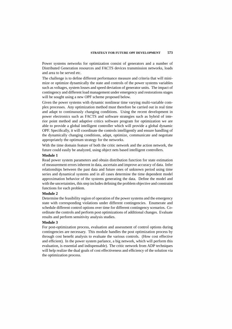
STRATEGY FOR FUTURE OPF DEVELOPMENT 573
Power systems networks for optimization consist of generators and a number ofDistributed Generation resources and FACTS devices transmission networks, loadsand area to be served etc.
The challenge is to define different performance measure and criteria that will mini-mize or optimize dynamically the state and controls of the power systems variablessuch as voltages, system losses and speed deviation of generator units. The impact ofcontingency and different load management under emergency and restorations stageswill be sought using a new OPF scheme proposed below.
Given the power systems with dynamic nonlinear time varying multi-variable com-plex processes. Any optimization method must therefore be carried out in real timeand adapt to continuously changing conditions. Using the recent development inpower electronics such as FACTS and software strategies such as hybrid of inte-rior point method and adaptive critics software program for optimization we areable to provide a global intelligent controller which will provide a global dynamicOPF. Specifically, it will coordinate the controls intelligently and ensure handling ofthe dynamically changing conditions, adapt, optimize, communicate and negotiateappropriately the optimum strategy for the networks.
With the time domain feature of both the critic network and the action network, thefuture could easily be analyzed, using object nets based intelligent controllers.
Module 1Read power system parameters and obtain distribution function for state estimationof measurement errors inherent in data, ascertain and improve accuracy of data. Inferrelationships between the past data and future ones of unknown period using timeseries and dynamical systems and in all cases determine the time dependent modelapproximation behavior of the systems generating the data. Define the model andwith the uncertainties, this step includes defining the problem objective and constraintfunctions for each problem.
Module 2Determine the feasibility region of operation of the power systems and the emergencystate with corresponding violations under different contingencies. Enumerate andschedule different control options over time for different contingency scenarios. Co-ordinate the controls and perform post optimizations of additional changes. Evaluateresults and perform sensitivity analysis studies.
Module 3For post-optimization process, evaluation and assessment of control options duringcontingencies are necessary. This module handles the post optimization process bythrough cost benefit analysis to evaluate the various controls. (How cost effectiveand efficient). In the power system parlance, a big network, which will perform thisevaluation, is essential and indispensable). The critic network from ADP techniqueswill help realize the dual goals of cost effectiveness and efficiency of the solution viathe optimization process.
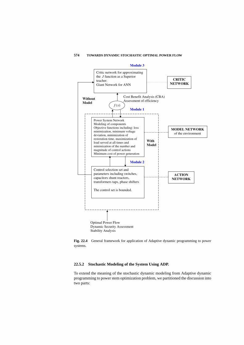
574 TOWARDS DYNAMIC STOCHASTIC OPTIMAL POWER FLOW
Critic network for approximating
the J function as a Superior
teacher.
Giant Network for ANN
Control selection set and
parameters including switches,
capacitors shunt reactors,
transformers taps, phase shifters
The control set is bounded.
Power System Network
Modeling of components
Objective functions including: loss
minimization, minimum voltage
deviation, minimization of
restoration time, maximization of
load served at all times and
minimization of the number and
magnitude of control actions
Minimum cost of power generation
With
Model
)(xf
ACTION
NETWORK
MODEL NETWORK
of the environment
Optimal Power Flow
Dynamic Security Assessment
Stability Analysis
CRITIC
NETWORK
Cost Benefit Analysis (CBA)
Assessment of efficiency Without
Model
Module 3
Module 1
Module 2
Fig. 22.4 General framework for application of Adaptive dynamic programming to powersystems.
22.5.2 Stochastic Modeling of the System Using ADP.
To extend the meaning of the stochastic dynamic modeling from Adaptive dynamicprogramming to power stem optimization problem, we partitioned the discussion intotwo parts:

STRATEGY FOR FUTURE OPF DEVELOPMENT 575
1. Dynamics (anticipatory) nature: In power systems, dynamics comes as a resultof the time dependence of the control set required for the optimization process.For any contingency such as changes in loading due to weather conditionswithin any time interval, adjustment of capacitor switching, transformer taps,minimizing voltage deviation using FACTS devices technology must be co-ordinated optimally for the efficient and cost effective operation of the powersystems.
2. Stochastic: probabilistic modeling of faults for reliability studies, and load-ing, as well as available transfer capability (ATC) of transmission lines areneeded to deal with unpredictable events such as faults on a line, equipmentfailure etc. these models have been addressed in power system literature overthe years. Moreover, weather variations effects such as solar radiation stormsbeing stochastic in nature affects thermal rating of transmission line. New andefficient computatitional techniques are therefore required for stochastic mod-eling of the new power system with new devices such as distributed generationsources and FACTS devices to ensure that priority of load, market structuresand planning of generation, transmission and distribution systems are welltaken care of.
In assessing the dynamic security of the system and identifying bottlenecks on trans-mission grids, these two qualities must be assessed.
Dynamic model of the environmentrefers to the actual power system to be opti-mized. In this case refers to model of the objective function, which could be eitherloss minimization, minimum voltage deviation, or cost function comparison. Thisleads to improvement of the conventional solution by taking it a step further andassessing the cost benefit analysis of the solution using the strategic utility function.
Assuming a stochastic model of the power system network due to change in load andother system dynamics given as:
X(t + 1) = F (X(t), u(t)) + noise,
where the only form of noise is error in the forecastX(t + 1).There are two main methods of handling the noise vector inF network namely thesimulated approach and the imputed noise approach.
Further assumptions are:
A set of vectors forX(t) for t = 1 throughT , the model networkF and the criticnetworkJ are kept constant. For the simulation approach, noise vectors are simulatedfor each value of and for each component of the vector noise a random value is pickedbased on the assumed probability distribution of the noise component. This procedureyields a set of vectors ofnoise(t) for all t. This set of noise data are held constant,a derivative is then calculated through one pass of the data with respect to a weightW ′
i ,
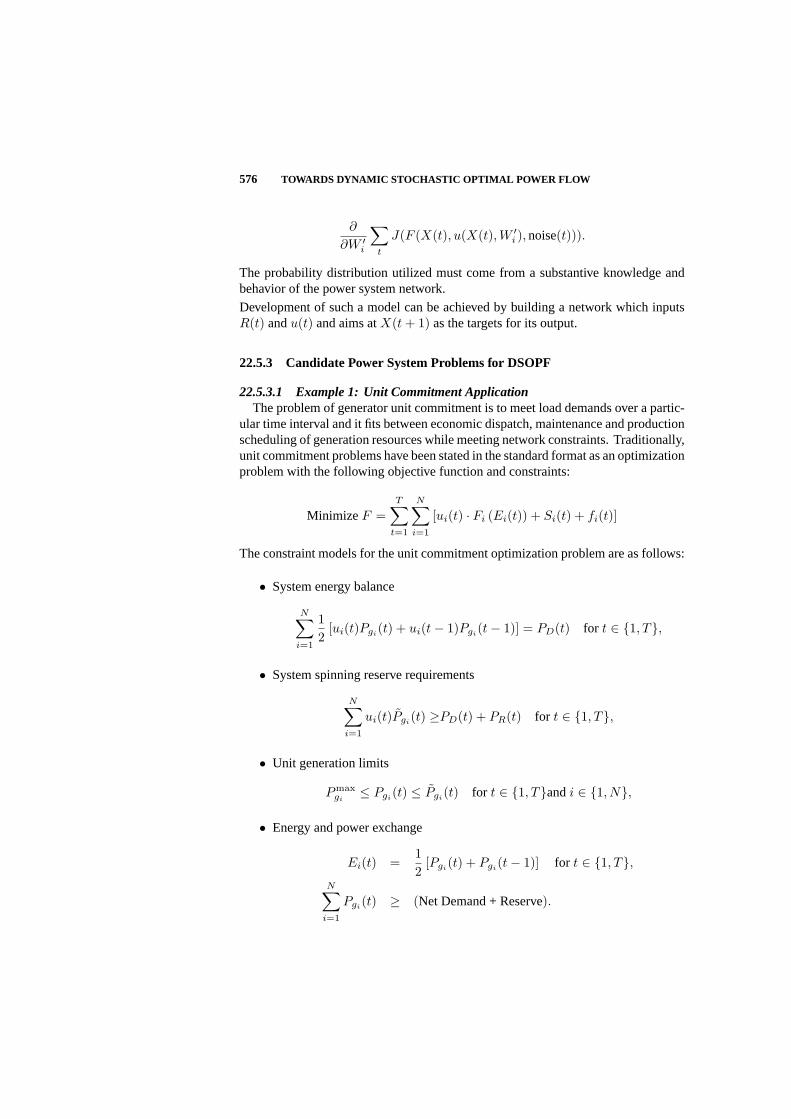
576 TOWARDS DYNAMIC STOCHASTIC OPTIMAL POWER FLOW
∂
∂W ′i
∑t
J(F (X(t), u(X(t),W ′i ), noise(t))).
The probability distribution utilized must come from a substantive knowledge andbehavior of the power system network.
Development of such a model can be achieved by building a network which inputsR(t) andu(t) and aims atX(t + 1) as the targets for its output.
22.5.3 Candidate Power System Problems for DSOPF
22.5.3.1 Example 1: Unit Commitment ApplicationThe problem of generator unit commitment is to meet load demands over a partic-
ular time interval and it fits between economic dispatch, maintenance and productionscheduling of generation resources while meeting network constraints. Traditionally,unit commitment problems have been stated in the standard format as an optimizationproblem with the following objective function and constraints:
Minimize F =T∑
t=1
N∑
i=1
[ui(t) · Fi (Ei(t)) + Si(t) + fi(t)]
The constraint models for the unit commitment optimization problem are as follows:
• System energy balance
N∑
i=1
12
[ui(t)Pgi(t) + ui(t− 1)Pgi(t− 1)] = PD(t) for t ∈ 1, T,
• System spinning reserve requirements
N∑
i=1
ui(t)Pgi(t) ≥PD(t) + PR(t) for t ∈ 1, T,
• Unit generation limits
Pmaxgi
≤ Pgi(t) ≤ Pgi(t) for t ∈ 1, Tandi ∈ 1, N,
• Energy and power exchange
Ei(t) =12
[Pgi(t) + Pgi(t− 1)] for t ∈ 1, T,N∑
i=1
Pgi(t) ≥ (Net Demand + Reserve).

STRATEGY FOR FUTURE OPF DEVELOPMENT 577
In case the units should maintain a given amount of reserve, its upper bounds mustbe modified accordingly. Therefore, we have:
Pmaxgi
= Pmaxgi
− P reservegi
Demand+ Losses ≤N∑
i=1
Pgi−
N∑
i=1
P reservegi
Ccold = CO(1− eαt) + CL
where
Ccold : Cost to start an off-line boiler;
α : Unit’s Thermal time constant;
t : Time in seconds;
CL : Labour Cost to up the units;
CO : Cost to start up a cold boiler.
Cbanked = CBt + CL
where
CB : Cost to start up a banked boiler;
t : Time in seconds.
Modeling in Unit CommitmentNomenclature:
F : Total operation cost on the power system;
Ei(t) : Energy output of theith unit at hourt;
Fi(Ei(t)) : Fuel cost of theith unit at hourt when the generated power is
equivalent toEi(t);N : Total number of units in the power system;
T : Total time under which Unit Commitment is performed;
Pgi(t) : Power output of theith unit at hourt;
Pgi(t) : Constrained generating capability of theith unit at hourt;
Pmaxgi (t) : Maximum power output of theith unit;
Pmingi (t) : Minimum power output of theith unit;
Si(t) : Start-up Cost of theith unit at hourt;
Fi(t) : Ramping Cost of theith unit at hourt;

578 TOWARDS DYNAMIC STOCHASTIC OPTIMAL POWER FLOW
PD(t) : Net system power demand at hourt;
PR(t) : Net system spinning reserve hourt;
λ(t) : Lagrangian Multiplier for the systempower balance constraint
at hourt;
µ(t) : Lagrangian Multiplier for the systemspinning reserveconstraint
at hourt;
ui(t) : Commitment state of theith unit at hourt;
The following optimization approaches are useful for dealing with the unit commit-ment problems:
• Dynamic Programming,
• Lagrangian Relaxation methods.
Due to the computational burden required for dynamic programming and the sub-sequent curse of dimensionality, the unit commitment problem becomes intractablehence approximate methods of computation are preferred for near-optimal or optimalsolutions.
Adaptive dynamic programming reinforces the learning process.
First we present an example for the unit commitment problem and then advance toapply the adaptive dynamic programming approach to the unit commitment problembased on the general framework of application to power systems.
Problem Statement
Find the optimal operation cost of a four units plant using dynamic programming tofind the optimum unit commitment schedules covering an 8-hour period.
Table 22.2 gives each unit characteristics including the maximum and minimumpower output of each unit, the incremental heat rate of fuels used, no load energyspecifying the amount of energy derivable from the unit when (on spinning), start upenergy required for boiler thermal systems).
Table 22.3 represents the load being served by the units over 2-hour period.
Table 22.4 represents the start up and down time required for the units.
The following table 22.5 gives the characteristic of all combinations needed as wellas the operating cost for each at the loads in the load data. An “∗” indicates that acombination can not supply the load. The starting conditions are (a) at the beginningof the1st period units 1 and 2 are up, (b) units 3 and 4 are down and have been downfor 8 hours.

STRATEGY FOR FUTURE OPF DEVELOPMENT 579
LIMITS OF INCREMENTAL NO LOAD START-UPUNIT THE UNIT HEAT RATE ENERGY ENERGY
Pmaxgi
Pmingi
(BTU/KWH) (MBTU/H) (MBTU/H)(MW) (MW)
1 500 70 9950 300 800
2 250 40 10200 210 380
3 150 30 11000 120 110
4 150 30 11000 120 110
Table 22.2 Load data (all time periods = 2h).
TIME t LOAD, PD(t) (MW)
1 600
2 800
3 700
4 950
Table 22.3 Load duration curve.
UNIT MINIMUM UP MINIMUM DOWNTIME (HR) TIME (HR)
1 2 2
2 2 2
3 2 4
4 2 4
Table 22.4 Start up and shut down.
Note: Fuel cost = 1 R/MBTU
Solution using dynamic programmingSTARTING CONDITION

580 TOWARDS DYNAMIC STOCHASTIC OPTIMAL POWER FLOW
Combination Units Operating cost forvarious load levels PD (MW)
1 2 3 4 600 700 800 950
A 1 1 0 0 6505 7525 * *
B 1 1 1 0 6649 7669 8705 *
C 1 1 1 1 6793 7813 8833 10475
Table 22.5 Operating cost for various load levels.
At the starting conditions, unit #1 and Unit #2 are up and Unit #3 and Unit #4 aredown for 8 hours.
(Load = 600MW)
l = 1,K = A
All the statesA, B, andC will be considered.
For stateA, we have
F (1, A) = minCmin(1, A) + S(0, A : 1, A) + Fmin(0, A)
.
The operating cost isCmin(1, A) = 6505($/h), the transition cost isS(0, A : 1, A) =0, but because we have two hours, the total cost should beF (1, A) = (2× 6505) +0 + 0 = 13010($)For stateB, we have
F (1, B) = minCmin(1, B) + S(0, A : 1, B) + Fmin(0, A)
.
The operating cost isCmin(1, B) = 6649($/h). In the transition from state A tostate B only unit #3 came on line, hence the transition cost will be the start up cost ofunit 3 coming on line, which is
S(0, A : 1, B) = start up cost of unit #3
= 110MBtu× 1.00$/MBtu
= $110.
T otalCost = F (1, B) = (2× 6649) + 110 + 0= $13408.
For stateC,
F (1, C) = minCmin(1, C) + S(0, A : 1, C) + Fmin(0, A)
.
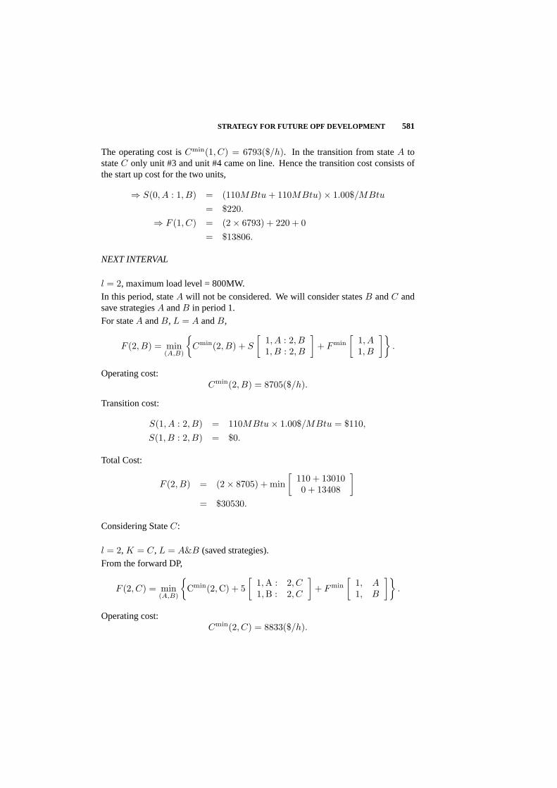
STRATEGY FOR FUTURE OPF DEVELOPMENT 581
The operating cost isCmin(1, C) = 6793($/h). In the transition from stateA tostateC only unit #3 and unit #4 came on line. Hence the transition cost consists ofthe start up cost for the two units,
⇒ S(0, A : 1, B) = (110MBtu + 110MBtu)× 1.00$/MBtu
= $220.
⇒ F (1, C) = (2× 6793) + 220 + 0= $13806.
NEXT INTERVAL
l = 2, maximum load level = 800MW.
In this period, stateA will not be considered. We will consider statesB andC andsave strategiesA andB in period 1.
For stateA andB, L = A andB,
F (2, B) = min(A,B)
Cmin(2, B) + S
[1, A : 2, B1, B : 2, B
]+ Fmin
[1, A1, B
].
Operating cost:Cmin(2, B) = 8705($/h).
Transition cost:
S(1, A : 2, B) = 110MBtu× 1.00$/MBtu = $110,
S(1, B : 2, B) = $0.
Total Cost:
F (2, B) = (2× 8705) + min[
110 + 130100 + 13408
]
= $30530.
Considering StateC:
l = 2, K = C, L = A&B (saved strategies).
From the forward DP,
F (2, C) = min(A,B)
Cmin(2, C) + 5
[1, A : 2, C1, B : 2, C
]+ Fmin
[1, A1, B
].
Operating cost:Cmin(2, C) = 8833($/h).

582 TOWARDS DYNAMIC STOCHASTIC OPTIMAL POWER FLOW
Transition cost:
S(1, A : 2, C) = (110MBtu + 110Mbtu)× 1.00$/MBtu = $220,
S(1, B : 2, C) = (110Mbtu + 110Mbtu) ∗ 1.00$/Mbtu = $110.
Total Cost:
F (2, C) = (2× 8833) + min[
220 + 13010110 + 13408
]
= 17666 + min
[1323013518
]
= $30896.
NEXT PERIOD
Maximum load level is 700MW. In this period we cannot shut down unit #3, since ifwe do (because it is possible to shut it down due to the minimum up/down time rules)that we cannot supply the load of 950 MW in the last 6-8 hrs. This is because unit 3will be needed but if it is down, then it has to be down for 4hrs to obey the minimumdown time period. Hence, we consider statesB andC only in this period.
StateB.K = B; l = 3; L = B&C.
Using the Forward DP,
F (3, B) = min(B,C)
Cmin (3, B) + 5
[2, B 3, B2, C 3, B
]+ Fmin
[2, B2, C
].
Operation Cost:
Cmin(3, B) = 7669$/h. - from table,
S(2, B : 3, B) = $0,
S(2, C : 3, B) = $0.
Total Cost:
F (3, B) = (2 ∗ 7669) + min[
3053030896
]
= $45868.
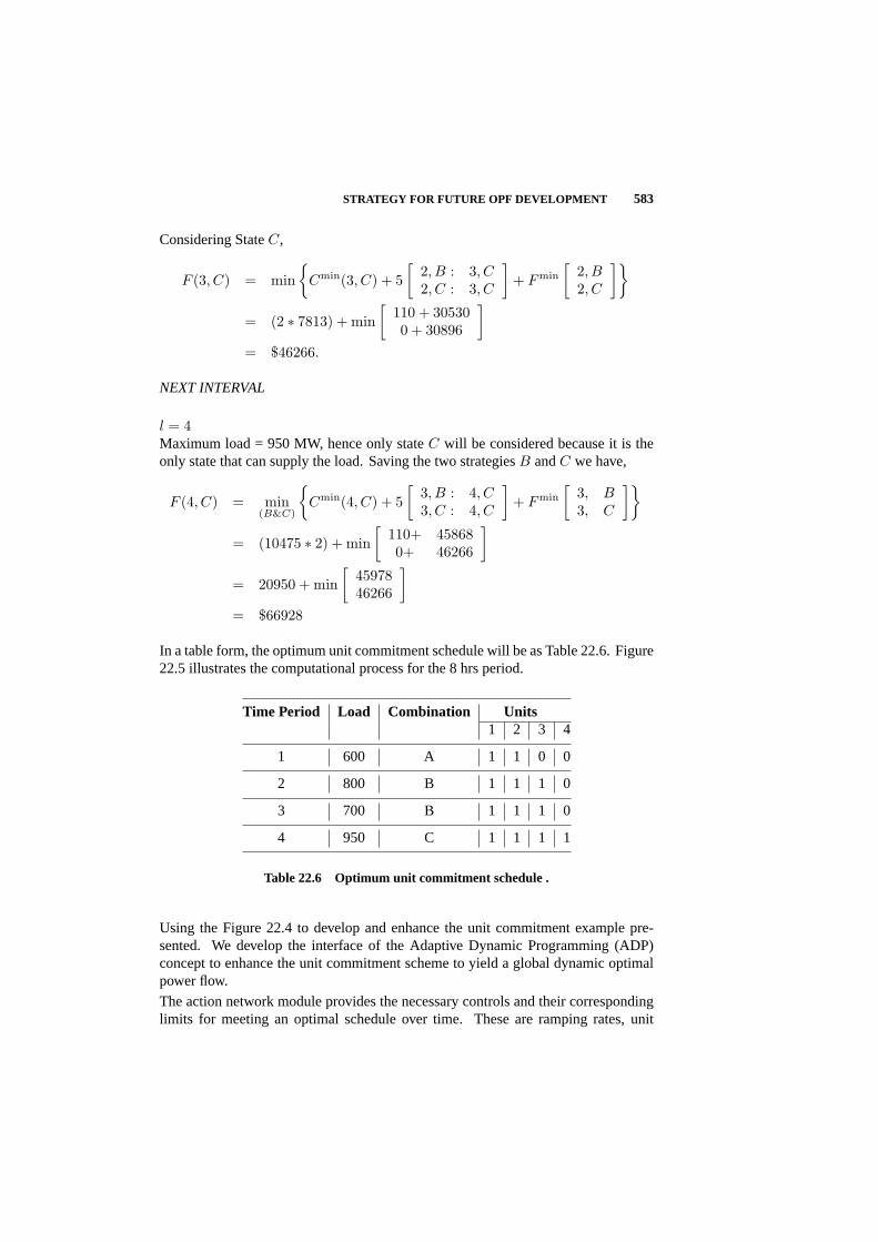
STRATEGY FOR FUTURE OPF DEVELOPMENT 583
Considering StateC,
F (3, C) = min
Cmin(3, C) + 5[
2, B : 3, C2, C : 3, C
]+ Fmin
[2, B2, C
]
= (2 ∗ 7813) + min[
110 + 305300 + 30896
]
= $46266.
NEXT INTERVAL
l = 4Maximum load = 950 MW, hence only stateC will be considered because it is theonly state that can supply the load. Saving the two strategiesB andC we have,
F (4, C) = min(B&C)
Cmin(4, C) + 5
[3, B : 4, C3, C : 4, C
]+ Fmin
[3, B3, C
]
= (10475 ∗ 2) + min[
110+ 458680+ 46266
]
= 20950 + min[
4597846266
]
= $66928
In a table form, the optimum unit commitment schedule will be as Table 22.6. Figure22.5 illustrates the computational process for the 8 hrs period.
Time Period Load Combination Units1 2 3 4
1 600 A 1 1 0 0
2 800 B 1 1 1 0
3 700 B 1 1 1 0
4 950 C 1 1 1 1
Table 22.6 Optimum unit commitment schedule .
Using the Figure 22.4 to develop and enhance the unit commitment example pre-sented. We develop the interface of the Adaptive Dynamic Programming (ADP)concept to enhance the unit commitment scheme to yield a global dynamic optimalpower flow.
The action network module provides the necessary controls and their correspondinglimits for meeting an optimal schedule over time. These are ramping rates, unit

584 TOWARDS DYNAMIC STOCHASTIC OPTIMAL POWER FLOW
Complete Solution: Up/Down Time minimum rules obeyed.
State Units TotalCombination 1 2 3 4 Capacity
C 1 1 1 1 1050
B 1 1 1 0 900
A 1 1 0 0 750
1 2 3 4 5 6 7 8 9
950 MW
Start
600 MW
800 MW 700 MW
The Optimum Path
Hour
46266 66928
4586830530
13010
Fig. 22.5 Computational process for the 8 hrs period.
generation, downtimes and uptimes, spinning reserve requirements, energy and powerexchange, unit’s availability etc. The purpose of the action network is to provide thecontrol variables needed for the optimization of the model objective functions as it istraditional done in ADP process.
At the model level in the frame work for the unit commitment problem consistingof the objective function and the constraints, the unit commitment problem is typi-cally optimized using Lagrange relaxation method or the well known dynamic pro-gramming or recently evolutionary programming and particle swarm programmingtechniques. The corresponding ADP approach either keeps the method or solvesthe model free approach using recurrent neural network techniques. The optimizedgeneration schedules are presented to the critic network to assess the achievement ofthe multi-objectives formulation in the model such as cost effectiveness, reliability,security and efficiency.
This evaluator feeds back the set of controls to the action network for readjustment andaims at improving the overall cost function and performance of the unit commitmentschedule. To account for the stochastic nature of load variation and network changes,the model is refined by the giant critic network to learn from these changes.

STRATEGY FOR FUTURE OPF DEVELOPMENT 585
22.5.3.2 Example 2: Application to Distribution System ReconfigurationDistribution networks are generally configured radially for effective and non-
complicated protection schemes. Under normal operation conditions, distributionfeeders may be reconfigured to satisfy the following objectives:
• Minimum distribution line losses
• Optimum voltage profile
• Relieve the overloads in the network.
While all load requirements and maintaining the radial structure of the network.Distribution reconfiguration application schemes are used to control switching oper-ations to clear the abnormal conditions or to improve service quality for a stresseddistribution system.
Minimize∑
ZbIb
Subject to[A]i = I
where
Zb : Impedance of the branch,
Ib : Complex current flow in the branchb,
i : m-vector of complex branch currents,
m : Total number of the branches,
I : n-vector of complex nodal injection currents.
n : Total number of network nodes,
A : Network incidence matrix, whose entries are
(ap, b) =
= 1 : if branchb starts from the nodep= −1 : if the branchb starts from the nodeb= 0 : if the branch is not connected to the nodep,
The problem of feeder reconfiguration for voltage deviation minimization couldbe studied using the 32-bus distribution network. This class of problem is solvedusing integer programming or heuristic programming. The problem can be cast inADP formulation and using the framework in Figure 22.4 to determine the optimumswitching sequences while minimizing losses and voltage deviation.
u(t) : Action vectors, open/close status for 37 switches
U(t) : The objective function

586 TOWARDS DYNAMIC STOCHASTIC OPTIMAL POWER FLOW
0
1
5
8
11
14
16
18
20
22
24
26
28
29
30
31
32
2
4
7
10
13
27
15
25
23
21
19
17
9
12
6
3
36
35
3337
34
Fig. 22.6 Bus Distribution System with 5 normally open switches.
r : Usual discount rate or interest rate that is needed only in infinite-time
horizon problems
J : Secondary or strategic utility function
X(t) : Real and active loads to the 32 buses and 5 normally open switches
To solve the reconfiguration problem we use the framework of ADP application topower systems distribution system reconfiguration problem is modeled as combi-natorial optimization with variables representing the switching status of equipment.The controls sequences in the action networks include capacitors, reactors, trans-former taps and phase shifters which are options available for reconfiguration of thesystem and amount of control offered by each equipment, which may be discrete orcontinuous.
As before the critic network evaluates the control set adopted for any contingencyand assigns cost and benefits derivable from such actions. At convergence usingthe classical or ADP based OPF we obtain the optimal load flow pattern resultsin minimum voltage deviation for the optimum reconfiguration under different coloading conditions and uncertainties
22.5.3.3 Example 3: Dynamic security assessment of the power systemsThe increasing complexity of power systems due to their growth and operation close
to designed limits, economic constraints and new regulations required for restruc-turing calls for the incorporation of dynamic security assessment into SupervisoryControl and Data Acquisition (SCADA) and Energy Management Systems (EMS).Current research employed methodologies of hybridized nature to handle the securityassessment of the power systems thereby improve the accuracy of existing tools usedin analyzing the system. These hybrid methods consists of time domain simulations

CONCLUSION 587
and transient energy functions as well as computational intelligence techniques suchas neural networks, fuzzy logic and genetic algorithms. Significant progress hadbeen made in this area of research making the analysis of security assessment online[13,14].
The classical method involves computation of critical energy, total energy systemat the instant of fault and then determine the stability margin which is based on thedifference between the critical energy and energy at fault clearing. The index varieswith topology changes and uncertainties in load. To achieve the desired stabilitycontrol actions are taken to reduce the system instability. This is a classic problem,which has been done using ANN for training and to assess the system conditions.The incorporation of this stability index as a constraint in OPF is being a researchinvestigation for now. The treads of SDOPF framework in Figure 22.4 is a candidateproblem for obtain assessment and profitability.
Finally, as we gain more experience and confidence in the application of ADP topower systems optimization problems several other challenging OPF problems willbe tested as part of an ongoing research investigation.
22.6 CONCLUSION
Optimal Power Flow (OPF) is one of the most important operational functions ofthe modern day energy management system. There are several objectives of optimalpower flow that must be considered simultaneously when determining an optimalcontrol stratrgy. The main drawbacks of conventional OPF tools is that they lackforesight, the ability to predict the future in terms of asset valuation and economicrate of return on investment; and lack of explicit optimization techniques to handleperturbation and noise, the power system is not static, but changing with respect toload demands at any given time period.
Approximate Dynamic Programming (ADP) is a computational intelligence tech-nique that can incorporate the time features required for the future. Dual HeuristicDynamic Programming (DHP), a class of ADP, can be used, with appropriate model-ing of the power system, to incorporate foresight and to enhance stochastic descrip-tion and prediction of the power network. This chapter has presented a method forincorporating DHP into an extension of OPF.

Bibliography
1. Thomas Miller III, Richard S. Sutton, and Paul J. Werbos,Neural Networksfor Control, a Bradford Book,MIT Press, Cambridge, Massachusetts, London,England.
2. P.J. Werbos, “Approximate Dynamic Programming for Real-Time Control andNeural Modeling,”Handbook of Intelligent Control, White and Sofge (Eds.),pp. 493–525, New York, NY, 1992.
3. G.K.Venayagamoorthy, R.G.Harley, and D.C.Wunsch, “Intelligent Control ofTurbogenerator Exciter/Turbine on the Electric Power Grid to Improve PowerGeneration and Stability,”Proceedings, ICPSOP 2002,Abuja, Nigeria.
4. D. Prokhorov, and D.C. Wunsch, “Adaptive Critic Designs”,IEEE Transactionson Neural Networks,vol. 8(5), pp. 997–1007.
5. J.A. Momoh, and J.Z. Zhu, “Improved Interior Point Method to OPF Problems,”IEEE Transactions PES,vol. 14, pp. 1114–1130, 1999.
588

23 Control, Optimization, Security,and Self-healing of BenchmarkPower Systems†
JAMES A. MOMOH and EDWIN ZIVINational Science Foundation U.S. Naval Academy
Editor’s Summary: This chapter presents several challenging and benchmarkproblems from the field of power systems. The first benchmark is the IEEE 118Bus commercial terrestrial Electrical Power System (EPS). The second benchmarkrepresents a finite inertia hybrid AC/DC shipboard Integrated Power System (IPS).The analytic utility and Navy benchmark models and their respective simulations havebeen experimentally validated, and have been used to determine system reliability,reconfigurability, stability and security. The challenge is to provide novel control andoptimization methods and tools to improve the quality of service despite natural andhostile disruptions under uncertain operating conditions. Along with these problemsseveral smaller problems are also presented which demonstrate different aspects ofthe challenges of power system control. The purpose of this chapter is formulationof problems that ADP methods could be applied to, therefore the emphasis is moreon detailed problem description and simulation, not on any particular solution.
23.1 INTRODUCTION
Market driven power system restructuring, along with advances in distributed gen-eration, energy conversion and protection technologies requires new control, sta-bilization and optimization techniques. Moreover, these systems are composed ofdynamically interdependent subsystems for which static and isolated design and op-timization may fail. For example, the need for robust, distributed infrastructures is
†The views expressed here are those of the authors, Momoh (on leave from Howard University), andZivi and not the official views of NSF and US Naval Academy.
589

590 CONTROL, OPTIMIZATION, SECURITY & SELF-HEALING OF BP SYSTEM
articulated by the Architectures for Secure and Robust Distributed Infrastructuresinitiative [1]:
“The major barrier constraining the successful management and design of large-scale distributed infrastructures is the conspicuous lack of knowledge about theirdynamical features and behaviors. Up until very recently analysis of systems suchas the Internet, or the national air traffic system, have primarily relied on the useof non-dynamical models, which neglect their complex, and frequently subtle, inher-ent dynamical properties. These traditional approaches have enjoyed considerablesuccess while systems are run in predominantly cooperative and “friendly” environ-ments, and provided that their performance boundaries are not approached. Withthe current proliferation of applications using and relying on such infrastructures,these infrastructures are becoming increasingly stressed, and as a result the incen-tives for malicious attacks are heightening. The stunning fact is that the fundamentalassumptions under which all significant large-scale distributed infrastructures havebeen constructed and analyzed no longer hold; the invalidity of these non-dynamicalassumptions is witnessed with the greater frequency of catastrophic failures in ma-jor infrastructures such as the Internet, the power grid, the air traffic system, andnational-scale telecommunication systems.”
The power industry is currently developing new technologies, architectures and con-trol strategies to achieve adaptable, efficient and secure power systems. In support ofthese efforts, two benchmark problems are presented herein. The first benchmark isa commercial terrestrial Electrical Power System (EPS). The second benchmark rep-resents a finite inertia hybrid AC/DC shipboard Integrated Power System (IPS). Theanalytic utility and Navy benchmark models and simulations have been experimen-tally validated and used to determine system reliability, reconfigurability, stabilityand security. The challenge is to provide novel control and optimization methods andtools to improve the quality of service despite natural and hostile disruptions underuncertain operating conditions.
This chapter presents two reference benchmark systems addressing two challengingproblems:
• Utility power system optimization for scheduling unit commitment subject tounit availability, dynamic response and transmission constraints.
• Maximizing continuity of service despite temporal and spatially clustered“bursts” of natural or hostile disruption.
Many of the control strategies, optimization techniques and learning agents presentedin this book have the potential to significantly improve the efficiency and depend-ability of the terrestrial Electric Power System and the shipboard Integrated PowerSystem.

DESCRIPTION OF THE BENCHMARK SYSTEMS 591
23.2 DESCRIPTION OF THE BENCHMARK SYSTEMS
Since objective benchmark problems with realistic constraints are often difficult toobtain, challenge problems are presented in terms of the two benchmark systems.The IEEE 118 BusEPS benchmark is representative of large commercial AC ter-restrial systems. The shipboard IPS benchmark provides a complementary isolatedmicro-grid containing solid-state power conversion, regulation and DC distribution.These benchmarks provide reliable, validated system models, assumptions and sim-ulations. Moreover, model complexity, convergence and numerical issues have beensuppressed in favor of facilitating the investigation of innovative control, optimiza-tion design and planning strategies for robust, high performance, self-healing powersystems.
23.2.1 General Introduction to Utility Power Systems
A typical power system consists of generation, transmission and distribution elements.The commercial benchmark system is theIEEE 118 Buselectric power system shownin Figure 23.1. Data for this benchmark is available fromhttp://www.ee.washington.edu/research/pstca/.Generally, utility systems share common fundamental characteristics including:
• Electric power is generated using synchronous machines that are driven bysteam turbines, gas turbines, hydro-turbines or internal combustion engines.
• Generated power is transmitted from generating sites over long distances toload centers that are spread over wide areas.
• Three phase AC systems comprise the main means of generation, transmissionand distribution of electric power.
• Tight voltage and frequency regulation is required to maintain high qualityproduct.
Electric power is produced at generating stations and transmitted to consumersthrough an intricate network involving transmission lines, transformers and switchingdevices. The following hierarchy is used to classify the transmission network: (1)Transmission system (2) Sub transmission system and (3) Distribution system.
The transmission system interconnects all major generating stations and main loadcenters in the system. It forms the backbone of the integrated power system andoperates at the highest voltage levels (typically, 230 kV and above). The generatorvoltages are usually in the range of 11 to 35 kV. These voltages are stepped up tothe transmission voltage level, and power is transmitted to transmission sub-stationswhere the voltages are stepped down to the subtransmission level at substations(typically, 69 kV to 138 kV). The generation and transmission subsystems are oftenreferred to as the bulk power system. The subtransmission system transmits power
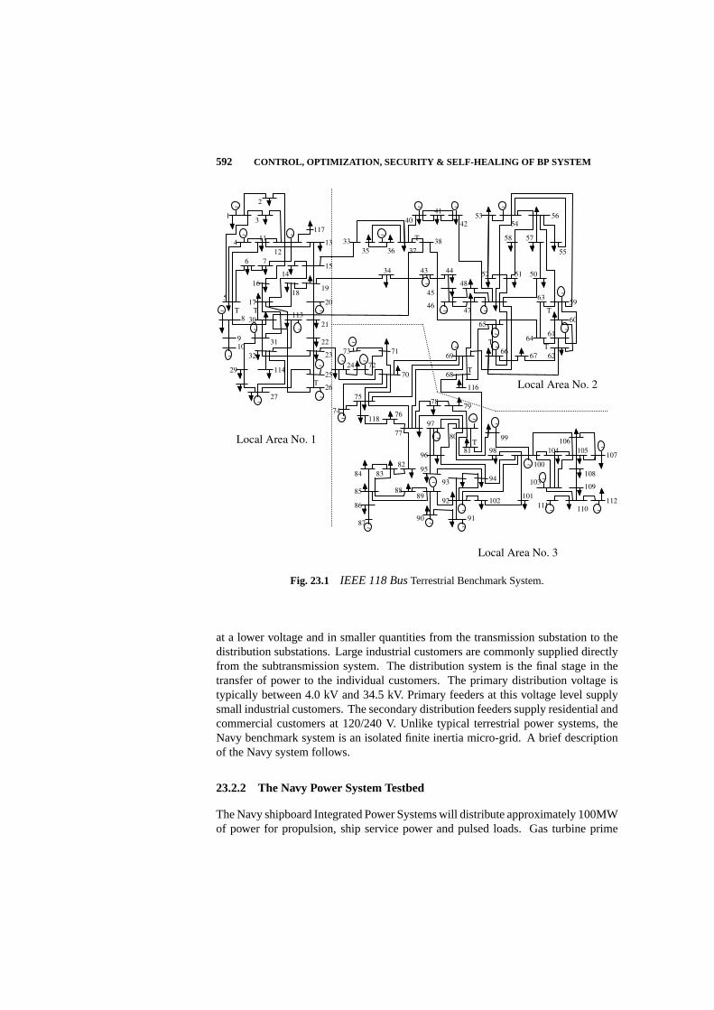
592 CONTROL, OPTIMIZATION, SECURITY & SELF-HEALING OF BP SYSTEM
TT
T
~
~ ~
~
~
~
~
~
~
~~
1
2
3
117
411
12
13
6 7
14
15
517
16
1819
20
8 30113
21
9
1031
32
22
23
29 11425
26
27
~
~
~
~
T
~
~
~
~
T
~
~
T~T
T
~
~ ~
~
~ ~~
T
~
~
~~
~
~
~
~
~ ~
33
35 36 37
38
40
41
42
53
54
56
58 57
55
34 43 44
45
46
48
47
52 51 50
6359
6065
6461
6269 676673 71
24 72
70 68
116
75
74
11876
77
7879
97
80 99
9681 98
100
104
106
105107
108
109
110
112
103
101
111
84 83
8295
9394
10292
91
85
86
87~
8889
90
Local Area No. 1
Local Area No. 2
Local Area No. 3
Fig. 23.1 IEEE 118 BusTerrestrial Benchmark System.
at a lower voltage and in smaller quantities from the transmission substation to thedistribution substations. Large industrial customers are commonly supplied directlyfrom the subtransmission system. The distribution system is the final stage in thetransfer of power to the individual customers. The primary distribution voltage istypically between 4.0 kV and 34.5 kV. Primary feeders at this voltage level supplysmall industrial customers. The secondary distribution feeders supply residential andcommercial customers at 120/240 V. Unlike typical terrestrial power systems, theNavy benchmark system is an isolated finite inertia micro-grid. A brief descriptionof the Navy system follows.
23.2.2 The Navy Power System Testbed
The Navy shipboard Integrated Power Systems will distribute approximately 100MWof power for propulsion, ship service power and pulsed loads. Gas turbine prime
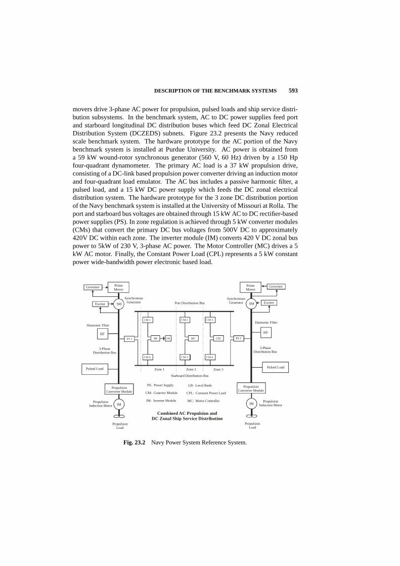
DESCRIPTION OF THE BENCHMARK SYSTEMS 593
movers drive 3-phase AC power for propulsion, pulsed loads and ship service distri-bution subsystems. In the benchmark system, AC to DC power supplies feed portand starboard longitudinal DC distribution buses which feed DC Zonal ElectricalDistribution System (DCZEDS) subnets. Figure 23.2 presents the Navy reducedscale benchmark system. The hardware prototype for the AC portion of the Navybenchmark system is installed at Purdue University. AC power is obtained froma 59 kW wound-rotor synchronous generator (560 V, 60 Hz) driven by a 150 Hpfour-quadrant dynamometer. The primary AC load is a 37 kW propulsion drive,consisting of a DC-link based propulsion power converter driving an induction motorand four-quadrant load emulator. The AC bus includes a passive harmonic filter, apulsed load, and a 15 kW DC power supply which feeds the DC zonal electricaldistribution system. The hardware prototype for the 3 zone DC distribution portionof the Navy benchmark system is installed at the University of Missouri at Rolla. Theport and starboard bus voltages are obtained through 15 kW AC to DC rectifier-basedpower supplies (PS). In zone regulation is achieved through 5 kW converter modules(CMs) that convert the primary DC bus voltages from 500V DC to approximately420V DC within each zone. The inverter module (IM) converts 420 V DC zonal buspower to 5kW of 230 V, 3-phase AC power. The Motor Controller (MC) drives a 5kW AC motor. Finally, the Constant Power Load (CPL) represents a 5 kW constantpower wide-bandwidth power electronic based load.
SM
PrimeMover
PrimeMover
PropulsionConverter Module
PropulsionConverter Module
HF HF
Pulsed Load Pulsed Load
Governor Governor
Exciter
PropulsionLoad
PropulsionLoad
3-Phase Distribution Bus
3-Phase Distribution Bus
PropulsionInduction Motor
PropulsionInduction Motor
SynchronousGenerator
SynchronousGenerator
Harmonic FilterHarmonic Filter
Combined AC Propulsion andDC Zonal Ship Service Distribution
SM SM
LBIM
CM 1
CM 4
MC
CM 6
CM 2
CPL
CM 3
CM 5
PS 1
Port Distribution Bus
Zone 1 Zone 2 Zone 3
Starboard Distribution Bus
PS: Power Supply CM: Conerter Module
IM: Inverter Module
LB: Local Bank CPL: Constant Power Load
MC: Motor Controller
Exciter
IMIM
Fig. 23.2 Navy Power System Reference System.

594 CONTROL, OPTIMIZATION, SECURITY & SELF-HEALING OF BP SYSTEM
23.3 ILLUSTRATIVE TERRESTRIAL POWER SYSTEM CHALLENGEPROBLEMS
The following power systems engineering problems have been chosen to illustratethe nature of problems encountered in the power industry and the limitations of thepresently available tools for analyzing the networks. Some of the referred texts forthis exercise are [2], [24]–[28]. The analyses of various problems feature the systemdescription, the topology, state variables, network constraints, the static and dynamicequations and network parameters.
Generalizing the standard power flow equations, allows static optimization strategiesto be developed solving the Optimal Power Flow (OPF) problem. Optimization isan essential tool to obtain large power systems that are: (1) affordable, (2) reliable,(3) secure and (4) economically sustainable. The ability to achieve this essentialOptimal Power Flow is limited by solution: (1) accuracy, (2) speed and (3) robustness.Optimization of system operation requires:
• Hourly “unit commitment” decisions regarding whether a unit is on or off at agiven hour.
• Hourly “hydrothermal problem” decisions that take advantage of hydroelectricplant generation flexibility to manage water reserve levels and improve systemperformance.
• Longer-term “maintenance-scheduling problem” decisions that minimize theproduction cost without violating system reserve requirements.
In the following, scaled down versions of 3-bus and 5-bus systems, representingrealistic systems, are presented to facilitate the discussions and the understanding ofpower system concepts. The three examples below address issues on (1) load flow(2) economic dispatch of generating units (3) transient stability of power system.
23.3.1 Load flow problem and solution
The power flow equations are expressed as follows:
S∗i = Pi − jQi = V ∗i
n∑
j=1
YijVj (23.1)
whereS∗i , P andQ represent the conjugate of the apparent power, the real power andthe reactive power, respectively. The real and reactive powers are computed from
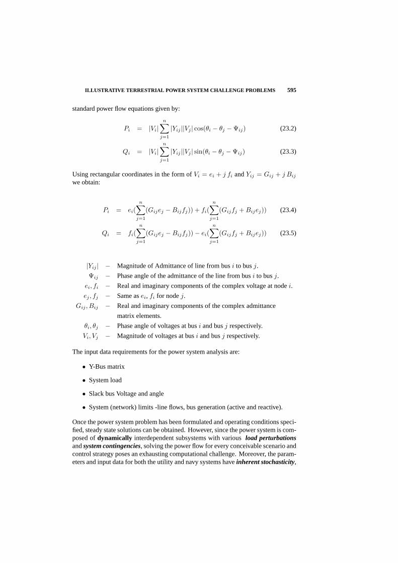
ILLUSTRATIVE TERRESTRIAL POWER SYSTEM CHALLENGE PROBLEMS 595
standard power flow equations given by:
Pi = |Vi|n∑
j=1
|Yij ||Vj | cos(θi − θj −Ψij) (23.2)
Qi = |Vi|n∑
j=1
|Yij ||Vj | sin(θi − θj −Ψij) (23.3)
Using rectangular coordinates in the form ofVi = ei + j fi andYij = Gij + j Bij
we obtain:
Pi = ei(n∑
j=1
(Gijej −Bijfj)) + fi(n∑
j=1
(Gijfj + Bijej)) (23.4)
Qi = fi(n∑
j=1
(Gijej −Bijfj))− ei(n∑
j=1
(Gijfj + Bijej)) (23.5)
|Yij | − Magnitude of Admittance of line from busi to busj.
Ψij − Phase angle of the admittance of the line from busi to busj.
ei, fi − Real and imaginary components of the complex voltage at nodei.
ej , fj − Same asei, fi for nodej.
Gij , Bij − Real and imaginary components of the complex admittance
matrix elements.
θi, θj − Phase angle of voltages at busi and busj respectively.
Vi, Vj − Magnitude of voltages at busi and busj respectively.
The input data requirements for the power system analysis are:
• Y-Bus matrix
• System load
• Slack bus Voltage and angle
• System (network) limits -line flows, bus generation (active and reactive).
Once the power system problem has been formulated and operating conditions speci-fied, steady state solutions can be obtained. However, since the power system is com-posed ofdynamically interdependent subsystems with variousload perturbationsandsystem contingencies, solving the power flow for every conceivable scenario andcontrol strategy poses an exhausting computational challenge. Moreover, the param-eters and input data for both the utility and navy systems haveinherent stochasticity,
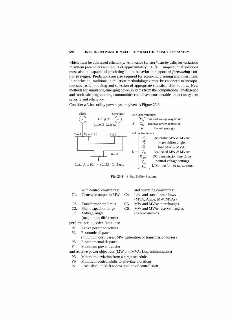
596 CONTROL, OPTIMIZATION, SECURITY & SELF-HEALING OF BP SYSTEM
which must be addressed efficiently. Allowance forstochasticitycalls for variationsin system parameters and inputs of approximately±10%. Computational solutionsmust also be capable of predicting future behavior in support offorecastingcon-trol strategies. Predictions are also required for economic planning and investment.In conclusion, traditional simulation methodologies must be enhanced to incorpo-rate stochastic modeling and selection of appropriate statistical distributions. Newmethods for simulating emerging power systems from the computational intelligenceand stochastic programming communities could have considerable impact on systemsecurity and efficiency.
Consider a 3-bus utility power system given as Figure 23.3:
Bus 1
2 2
(0.100 0.15) .
P jQ
j p u
+ =
+
Bus 2
V1 = 1 ∠ 0
~ ~
3 3Load: (0.16 0.18) .P jQ j p u+ = − +
Slack Generator
Bus 3
with state variables:
Bus load voltage magnitude
Reactive power generation
Bus voltage angle
D
G
VX Q
θ
=
and control inputs:
( )
generator MW & MVAr phase shifter angles load MW & MVAr
load shed MW & MVAr DC transmission line flows
control voltage settingsLTC transformer tap set
G
i
ij
D
D DC
set
set
P
P
PUP
VT
θ
=
tings
Fig. 23.3 3-Bus Utility System.
with control constraints: and operating constraints:C1. Generator output in MW C4. Line and transformer flows
(MVA, Amps, MW, MVAr)C2. Transformer tap limits C5. MW and MVAr interchangesC3. Shunt capacitor range C6. MW and MVAr reserve marginsC7. Voltage, angle (fixed/dynamic)
(magnitude, difference)performance objective functions:
P1. Active power objectivesP2. Economic dispatch
(minimum cost losses, MW generation or transmission losses)P3. Environmental dispatchP4. Maximum power transfer
and reactive power objectives (MW and MVAr Loss minimization)P5. Minimum deviation from a target scheduleP6. Minimum control shifts to alleviate violationsP7. Least absolute shift approximation of control shift.

ILLUSTRATIVE TERRESTRIAL POWER SYSTEM CHALLENGE PROBLEMS 597
with the following initial conditions:IC1. Vslack = 1∠0p.u. : Slack bus voltageIC2. pD : Total system loadIC3. pG : Generator (PV) active power generationIC4. |VG| : Magnitude of generator (PV) bus voltage
23.3.2 Optimization Problem (minimization of cost of generation)
Optimization problems involve minimization of functions with both equality andinequality constraints. Consider the following power system optimization problemgeneral formulation:
Minimize the functionf(x, u)subject to: g(x, u) = 0
h(x, u) ≤ 0(23.6)
wherex andu are the state and control variables of the power system. In solving thisproblem, the Lagrangian is formulated and the Kuhn-Tucker conditions of optimalityfor first order derivatives as well as second order derivatives are invoked to obtain thegeneral solution.
Power Systems Example on Optimization [2]The parameters of a 5-bus system are given in Table 23.1 and the cost functions indollars per hour are:
F1 = 0.0060P 21g + 2.0P1g + 140 (23.7)
F2 = 0.0075P 22g + 1.5P2g + 120 (23.8)
F3 = 0.0070P 23g + 1.8P3g + 80 (23.9)
assuming that0.95 p.u. ≤ Vi ≤ 1.05 p.u.; i = 1, ... Nbus. Assuming all genera-tors are rated at 200 MW, you can use the initial generation schedule with:
• The OPF program to obtain the absolute minimum cost of this system as wellas the real and reactive generation schedule.
• The OPF program to obtain the loss minimum of this system, the reactivepower of generation, and the optimal voltage profile.
Solution to a Deterministic Optimization Problem
The optimization problem is solved using a Quadratic sensitivity program based onLagrangian approach. From the OPF program, we obtain the following optimalvalues ofP , Q andV :

598 CONTROL, OPTIMIZATION, SECURITY & SELF-HEALING OF BP SYSTEM
Bus Code From Bus i to Bus j
Line Impedance pu
½ Line Charging Susceptance (pu)
Line Limits (MW)
1 2 0.02 + j0.06 J0.030 30 1 3 0.08 + j0.24 J0.025 40 2 3 0.06 + j0.18 J0.020 50 2 4 0.06 + j0.18 J0.020 80 2 5 0.04 + j0.12 J0.015 40 3 4 0.01 + j0.03 J0.010 180 4 5 0.08 + j0.24 J0.025 120
Table 23.1 5-Bus System Impedance and Line Charging Data.
Bus Voltage, Vi
iiVV
Power Generation Load Level Bus i
Magnitude
(pu)
Angle
(degrees)
Pgi
(MW)
Qgi
(MVAr)
Pload
(MW)
Qload
(MVAr)
1 1.060 0.0 98.4 - 0 0
2 1.056 -2.27 40.0 23.2 20 10
3 1.044 -3.69 30.0 30.0 45 15
4 1.041 -4.16 0.0 10.0 40 5
5 1.030 -5.35 0.0 0.0 60 10
Table 23.2 5-Bus Initial Generation Schedule.
• Absolute minimum cost = 2.7403Pg1 = 97.48MW,Pg2 = 40.00MW andPg3 = 30.00MWQg1 = -17.86MVAr,Qg2 = -0.260MVAr andQg3 = 33.94MVAr
• Loss minimum = 0.024763,|v4| = 1.04535 pu,|v5| = 1.02052 pu,Qg1 =-18.87MVAr andQg2 = 1.38MVAr.
The objective of power system optimization problems is to minimize the economicdispatch (minimum cost losses); MW generation or transmission losses; environmen-tal dispatch; maximum power transfer; minimum deviation from a target schedule;minimum control shifts to alleviate violations; and/or least absolute shift approxima-tion of control shift. Power system optimization problems have been solved using avariety of methods with various efficiencies measured in terms of reliability, speedof operation, flexibility, and maintainability. However, some methodologies areonly suitable for particular objective functions. Robust, multi-objective optimizationmethodologies are needed.
To date, Lagrangian and other optimization approaches have focused on the solutionto steady-state problems in which the load and network parameters are assumedconstant. In reality, the system is a complex dynamically interdependent systemsubjected to uncertainty due to time varying loads, parameter changes, disturbancesand noise. Increased use of solid-state based technologies, such as Flexible AC

ILLUSTRATIVE TERRESTRIAL POWER SYSTEM CHALLENGE PROBLEMS 599
Transmissions Systems (FACTS) will continue to inject additional noise. The presentoptimal power flow methods perform creditably in addressing the problems posedso far. However, simplifying assumptions to ease the computational burden ofexisting solutions limits the applicability of present work to solve the ever-increasingcomplexity in power systems. One possible extension of present methods would bethe introduction of stochastic optimal power flow tools that are capable of handlingfuture uncertainties over time.
23.3.3 Transient Stability Problem
Transient stability in power systems [3, 4] is concerned with the system’s ability toremain in synchronism following a major disturbance such as a line outage. Protectiverelays are placed strategically throughout the system to detect faults and to triggerthe opening of circuit breakers to isolate the fault. Therefore, the power systemcan be considered as going through changes in configuration in three stages, frompre-fault, fault-on, to post-fault systems. There are several approaches to solvingthe angle stability problem, including: (1) the Transient Energy function method,(2) Partial Energy function approach, and (3) the Hybrid method. In the TransientEnergy function method, the energy margin is obtained as the difference between thesystem’s transient energies, e.g. the difference between the potential energy of thesystem at the controlling unstable equilibrium point (UEP) and the kinetic energygained as a result of the disturbance. In the Transient Energy function method, thenormalized difference between the system energy at fault clearing and the energy atthe controlling UEP (the normalized energy margin [EM]) is used as the index ofstability. The system is stable if EM is positive and it is unstable if EM is negative.EM analysis also provides useful information leading to the effective application ofcontrol actions.
This section provides the mathematical formulation of Transient Energy functionmethod. Generally, a multi-machine system is represented by a set of differentialequations of the form:
δ = ω (23.10)
Mω = Pm − Pe (23.11)
T′doE
′q = Efd − E
′q + Id(Xd − X
′d) (23.12)
T′doEd = −Ed − Iq(Xq −X
′q) (23.13)
TexEfd = −Efd + Kex(Vref − Vt) (23.14)
where:

600 CONTROL, OPTIMIZATION, SECURITY & SELF-HEALING OF BP SYSTEM
E′q − Vq = IdX
′d + Iqrs (23.15)
E′d − Vd = −IqX
′q + Idrs (23.16)
δ : Rotor or torque angle.
δ : First derivative of the rotor angle w.r.t time.
ω : Angular speed of rotor.
ω : First derivative of the angular speed w.r.t time (angular acceleration).
Xl : Leakage reactance.
E′d : d-axis transient generated voltage.
E′fd : d-axis transient field voltage.
ra : Armature resistance.
Vt : Terminal voltage of the generator.
Xd : d-axis synchronous reactance.
X′d : d-axis transient reactance.
Id : d-axis current.
Iq : q-axis current.
T′do : d-axis open circuit transient time constant.
Xq : q-axis synchronous reactance.
X′q : q-axis transient reactance.
T′qo : q-axis open circuit transient time constant.
Tex : Excitation system time constant.
Vref : Referenced voltage.
The electrical power transmitted from each generator to the rest of the system iscalculated using the following equations:
Paj = Pmj − Pej − Mj
MTPCOI (23.17)
where:
PCOI =NR∑
j=1
Pmj − Pej ; MT =NR∑
j=1
Mj

ILLUSTRATIVE TERRESTRIAL POWER SYSTEM CHALLENGE PROBLEMS 601
and:
Pmj = Mechanical power of the j-th generator
Pej = Electrical power output of the j-th generator
M = Rotor Inertia;NR = number of Rotors
The expression can be re-written as:
Paj = Pj −NR∑k=1k 6=j
(Cjk sin θjk + Djk cos θjk)−ND∑
l=1
(Cjl sin θjl + Djl cos θjl),
(23.18)
where:
θi = Generator rotor angle;θj = Angle of converter AC bus
Pj = Pmj − E2j Gij ; Cjk = EjEkBjk ; ND = number DC bu
Djk = EjEkGjk ; Cjl = EjVlBil ; Djl = EjElGjl;
θjk = θj − θk; θjl = θj − θl
j, k = Generator internal nodes;l = Converter bus (AC side);
ωj = Machine rotor speed.
Computation of the Systems Energy Margin
The EM computation involves calculating the kinetic energy (KE) and potentialenergy (PE) terms. The total KE is computed from the speeds of all machines atclearing:
KE =12
∑
i
Miω2i . (23.19)
To account for the fact that not all the kinetic energy at the end of the disturbancecontributes to system separation, the concept of corrected kinetic energyKEco hasbeen introduced as:
KEcorr =12Meqω
2eq. (23.20)
where:
Meq =McrMsys
Mcr + Msys; andωeq = ωcrωsys.
The inertial center of the group of machines whose rotor angles have advancedbeyond 90 degrees at the controlling UEP has inertiaMcr and angular speedωcr.The corresponding terms for the rest of the generators areMsys and ωsys. The
602 CONTROL, OPTIMIZATION, SECURITY & SELF-HEALING OF BP SYSTEM
Potential Energy margin (PE) between clearing,θcl, and the unstable equilibriumpoint,θu, is given by:
PE =∑
i
θui∫
θcli
(Pmi − Pei) dθi. (23.21)
In the reduced formulation, PE can be divided into three components: (i) the positionenergy associated with the constant mechanical power output and shunt admittancesat the machine internal buses: (ii) the magnetic energy associated with the linesusceptances of the network; and (iii) the dissipation energy associated with thetransfer conductance of the reduced network. The dissipation term consists of a pathdependent integral, for which a closed form expression has been previously obtainedusing a linear angle trajectory betweenθcl andθu [24]. The computation of PE isformulated as an ordinary differential equation problem of the form:
yi = (Pmi − Pei)(θui − θcl
i ) (23.22)
θi = (θui − θcl
i ). (23.23)
This formulation is subject to the network power flow equations. The set ofdifferential-algebraic equations is solved in the time interval 0.0 to 1.0, using thesame variable-step, variable order integration routine used to determine the fault-ontrajectory, to obtain the potential energy margin to any desired degree of accuracy.
At the end of the integration process, PE is computed as:
PE =∑
i
yi, (23.24)
where the EM with KE correction is obtained from:
∆V =PE −KEcorr
KEcorr. (23.25)
The energy margin determines the stability of the system as follows:
If ∆V > 0.0 then, the system is stable
If ∆V = 0.0 Undetermined
If ∆V < 0.0 System is Unstable
Using the above equations, the stability analysis is computed for each of the machinesand if the energy margin is positive for all the generators, then the system is stable.Otherwise the system is unstable. In the TEF computation, the critical clearing time(Tcl) used is 0.1 seconds; this gives the speed and angle at a considerable operating

ILLUSTRATIVE TERRESTRIAL POWER SYSTEM CHALLENGE PROBLEMS 603
level.
Example on Transient Stability Analysis
A one-line diagram of the previous 3-Bus power system is as presented below asFigure 23.4. The system is subjected to a 3-phase fault on bus 2. The fault is clearedafter 0.1 seconds. Determine whether or not the system is stable after the fault iscleared.
Transient Stability Analysis Solution
The power generation at bus 2 and slack bus voltage magnitude and angle are givenin Figure 23.4. The line data and results are given below. Since PE is bigger than KEthroughout the cycle, the system is “transient” stable.
Bus 1
2 2
(0.100 0.15) .
P jQ
j p u
+ =
+
Bus 2
V1 = 1 ∠ 0
~ ~
3 3Load: (0.16 0.18) .P jQ j p u+ = − +
Slack Generator
Bus 3 3-phase fault on Bus # 2
Fig. 23.4 A 3-Bus Utility System with Bus 2 under 3-phase faulted condition.
The main concern in transient stability is the need for synchronism of AC systemsynchronous machines. If a system becomes unstable, at least one rotor anglebecomes unbounded with respect to the rest of the system. In transient stability,primary component to be modeled is the synchronous generators and the typical timeframe of concern 1 to 30 seconds. The objectives of power system transient stabilityare:
• Minimize of disturbance severity and duration.
• Increase forces restoring synchronism.

604 CONTROL, OPTIMIZATION, SECURITY & SELF-HEALING OF BP SYSTEM
3-Bus Transient Stability Line Data Line # From To R X Shunt
1 1 2 .05000 .22000 .080 2 2 3 .02500 .25000 060 3 1 3 .10000 .18000 .110
Pre-fault Bus Voltage Results
Bus # Voltage Magnitude Bus Angle 1 1.000 .0000 2 1.046 -.0092 3 1.024 -.0291
Unstable & Stable Equilibrium Points Bus # S.E.P U.E.P
1 .8747 2.2669 2 .5009 2.6406
Potential Energy (P.E) and Kinetic Energy (K.E) versus Time
-0.02
0
0.02
0.04
0.06
0 0.5 1 1.5
Time is seconds
P.E
and K
.E in
p.u
. K.E. |
P.E.
Fig. 23.5 3-Bus Energy Margin simulation results.
• Reduce the accelerating torque by reducing input mechanical power.
• Reduce the accelerating torque by applying artificial load.
Accurate analytical transient analysis results are critical for optimal operation of thepower system.
Relevance
Transient stability analysis using the energy margin approach provides an excellentanalysis of the power system following a disturbance. The results can be appliedto stability constrained optimal power flow. This type of OPF can be used in theenhancement of the power systems operation depending on the type of objectivefunction and controls being considered. There are several computational tools foranalyzing the transient stability of the system including EMTP (ElectromagneticTransient Program), HUTSP (Howard University Transient Stability Program), andEPRI-based PSAP packages. Most, if not all, of these programs do not handle theproblems of noise and complexity introduced due to the introduction of new technol-ogy such as FACTS devices and load regulation devices.

ILLUSTRATIVE EXAMPLE OF PS PROBLEMS USING NS SYSTEMS 605
Extensions
The use of the Energy Margin approach for solving transient stability problemshas been very successful in transient stability analysis. However, future of electricpower systems require new computational tools such as ADP for achieving improvedperformance that can incorporate increased non-linearity, noise, complexity anduncertainty.
The scalability of the new tools developed using ADP concepts will enhance workingmodels for analysis and controls for optimum performance of the navy ship systemsas well. We discuss herein the solved examples of the benchmark systems and discussareas of research grand challenges for future research.
23.4 ILLUSTRATIVE NAVY POWER SYSTEM CHALLENGEPROBLEMS
Isolated power electronics based electrical distribution systems are becoming in-creasingly common for renewable and mobile applications including air, land, andsea vehicles. In this section, three methods for analyzing the stability of powerelectronics based power distribution systems are reviewed and applied to the zonalDC distribution portion of the Navy benchmark system originally presented in Figure23.2 and documented in [5, 6, 7]. Each of these methods has practical limitations,which limit their applicability to real world systems. The challenge involves us-ing ADP methods for online system stability monitoring and augmentation despiteuncertain and disruptive operating conditions.
As shown in Figure 23.6, this DC zonal distribution testbed consists of two AC toDC power supplies feeding port and starboard DC distribution buses.
Each of three load distribution zones is fed from both the port and starboard DCdistribution buses via load sharing DC to DC converters. Note that diodes prevent afault in one bus from being fed by the opposite bus. Zonal loads are represented by anInverter Module (IM), a motor controller (MC), and a Constant Power Load (CPL).The DC zonal distribution hardware testbed was developed by the U.S. Navy andthe Energy Systems Analysis Consortium (ESAC) and is located at the University ofMissouri at Rolla.
These power electronics based systems facilitate a high degree of automation andoffer nearly instantaneous reconfiguration capabilities. Moreover, power electronicconverters can provide excellent regulation of their output objectives. For example,the DC to DC converter, shown in Figure 23.7, can maintain an essentially constantoutput voltage regardless of input disturbances. From a load regulation perspective,this property is highly desirable. However, Eqs. (23.26) and (23.27) show thatthis constant power demand causes the converter incremental input impedance withrespect to input voltage to be negative. This negative incremental input resistancehas an undesirable destabilizing effect on the interdependent overall power systemdynamics.
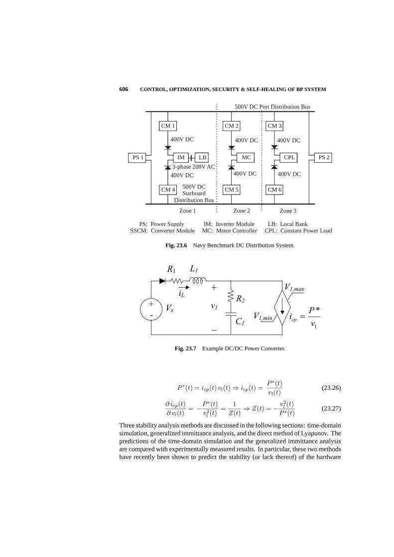
606 CONTROL, OPTIMIZATION, SECURITY & SELF-HEALING OF BP SYSTEM
PS 1 LBIM
CM 1
CM 4
MC
CM 6
CM 2
CPL
CM 3
CM 5
PS 2
500V DC Port Distribution Bus
Zone 1 Zone 2 Zone 3
500V DC Starboard
Distribution Bus
PS: Power SupplySSCM: Converter Module
IM: Inverter ModuleMC: Motor Controller
LB: Local Bank CPL: Constant Power Load
400V DC 400V DC
400V DC 400V DC
400V DC
400V DC
3-phase 208V AC
Fig. 23.6 Navy Benchmark DC Distribution System.
Fig. 23.7 Example DC/DC Power Converter.
P ∗(t) = icp(t) vl(t) ⇒ icp(t) =P ∗(t)vl(t)
(23.26)
∂ icp(t)∂ vl(t)
= −P ∗(t)v2
l (t)=
1Z(t)
⇒ Z(t) = − v2l (t)
P ∗(t)(23.27)
Three stability analysis methods are discussed in the following sections: time-domainsimulation, generalized immittance analysis, and the direct method of Lyapunov. Thepredictions of the time-domain simulation and the generalized immittance analysisare compared with experimentally measured results. In particular, these two methodshave recently been shown to predict the stability (or lack thereof) of the hardware
ILLUSTRATIVE EXAMPLE OF PS PROBLEMS USING NS SYSTEMS 607
test system [8]. A non-linear Lyapunov method using polytopic modeling techniquesis also presented. The DC stability analysis concludes with consideration of thelimitations of existing methods and opportunities for new ADP based analysis.
23.4.1 Preliminaries
DC Stability DefinitionsAlthough the definitions of an equilibrium point, an operating point, and of stabil-ity are crisply defined mathematically, some clarification is required for physicalsystems. In a model detailed enough to portray the switching action of the powersemiconductors, many of the state variables continue to cyclically change even understeady state conditions. Herein, an equilibrium point is a point at which the fast ordynamic average of the derivatives of the state variables is zero [9]. An operatingpoint is defined as an equilibrium point about which the system is being studied. Ifconditions are such that there is only one possible equilibrium point then these termsbecome synonymous. An operating point of the system model is said to be locallystable if, when perturbed from an operating point by a small amount, the systemmodel returns to that operating point. An operating point of the system model issaid to be globally stable if the operating point can be perturbed by any amount andstill return to that operating point. A DC power system is said to be locally stableabout an operating point if the system voltages and currents vary only at the forcingfrequencies associated with the switching of the power semiconductors and that theaverage values of these variables is such that all power converters are operating prop-erly. In other words, the system is said to be stable if, neglecting switching inducedripple, the voltages and currents are constant in the steady-state and the level of thesevoltages and currents is such that all converters are operating in their intended modesof operation. These comments with regard to stability are intended for informaldiscussion only. For a thorough and rigorous discussion, the reader is referred to [10]and [11].
DC System OperationReturning to the system, diagrammed in Figure 23.6, the two AC to DC powersupplies (PS1 and PS2), independently feed the port and starboard DC distributionbuses. Each zone is fed by port and starboard converter modules (CM), which usevoltage droop to share power. Diodes prevent a fault in one bus from being fed bythe opposite bus. The three characteristic loads consist of an inverter module (IM)that in turn feeds an AC load bank (LB), a motor controller (MC), and a genericconstant power load (CPL). Robustness in this system is achieved as follows. First,in the event that either a power supply fails, or a distribution bus is lost, the otherbus will pick up full system load without interruption in service. Imposing currentlimits on the converter modules mitigates faults between the converter module anddiode and as before, the opposite bus can supply the zone. Finally, faults within thecomponents are mitigated through the converter module controls.

608 CONTROL, OPTIMIZATION, SECURITY & SELF-HEALING OF BP SYSTEM
Operating the PS1 and PS2 power supplies in an uncontrolled rectifier mode resultsin the configuration given in Figure 23.8. The primary side AC voltage is a nearlyideal 480 V l-l rms source at 60 Hz. The transformer parameters are: primary leak-age inductance: 1.05 mH, primary winding resistance: 191 mΩ, secondary leakageinductance: 1.05 mH, secondary winding resistance: 191 mΩ, magnetizing induc-tance: 10.3 H and primary to secondary turns ratio of 1.30. All of these parametersapply to the wye-equivalent T-equivalent transformer model and are referred to theprimary winding. Finally, the DC link inductance,Ldc, is 9.93 mH, the resistance ofthis inductance,rLdc
, is 273 mΩ, the DC capacitor,Cdc, is 461 mF, and the effectiveseries resistance of the DC capacitor,rCdc
, is 70 mΩ. This capacitor is removed forsome studies as noted.
Fig. 23.8 AC to DC Power Supply.
The converter modules regulate the flow of power from the DC distribution buses intoeach zone. The circuit diagram is provided in Figure 23.9. Although the parametersvary from converter module to converter module, typical converter module parametersare: rCin = 1078 mΩ, Cout = 454µf , rCout = 70 mΩ, rLout = 101 mΩ.
Fig. 23.9 DC to DC Converter Module Circuit Diagram.
The experimentally validated converter module controller is presented in Figure 23.10and Table 23.3. The commanded output voltage isv∗out and the commanded inductorcurrent isi∗l . This current command, in conjunction with the measured currentil isused by a hysteresis modulator so that the actual current closely tracks the measuredcurrent. The undesirable constant power destabilizing effect of negative incremental
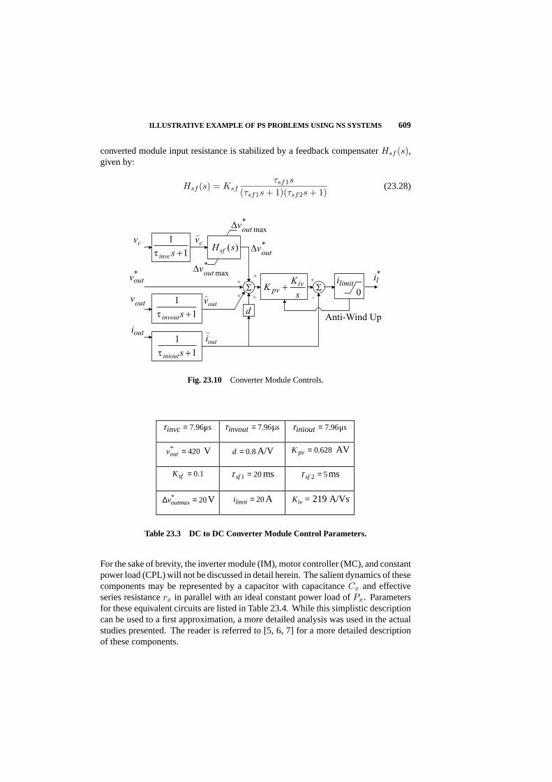
ILLUSTRATIVE EXAMPLE OF PS PROBLEMS USING NS SYSTEMS 609
converted module input resistance is stabilized by a feedback compensaterHsf (s),given by:
Hsf (s) = Ksfτsf1s
(τsf1s + 1)(τsf2s + 1)(23.28)
Fig. 23.10 Converter Module Controls.
s96.7=invcτ s96.7=invoutτ s96.7=inioutτ
420* =outv V 8.0=d A/V 628.0=pvK AV
1.0=sfK 201 =sfτ ms 52 =sfτ ms
20* =∆ outmaxv V 20=limiti A ivK = 219 A/Vs
Table 23.3 DC to DC Converter Module Control Parameters.
For the sake of brevity, the inverter module (IM), motor controller (MC), and constantpower load (CPL) will not be discussed in detail herein. The salient dynamics of thesecomponents may be represented by a capacitor with capacitanceCx and effectiveseries resistancerx in parallel with an ideal constant power load ofPx. Parametersfor these equivalent circuits are listed in Table 23.4. While this simplistic descriptioncan be used to a first approximation, a more detailed analysis was used in the actualstudies presented. The reader is referred to [5, 6, 7] for a more detailed descriptionof these components.

610 CONTROL, OPTIMIZATION, SECURITY & SELF-HEALING OF BP SYSTEM
Component F,xC m,xr kW,xP
IM 590 127 4.69
MC 877 105 2.93
CPL 374 189 5.46
Table 23.4 Equivalent Load Parameters.
Using this test system, two scenarios are studied. For each case, it is assumedthat the starboard bus is out of service due to a fault and that the remainder of thesystem is being fed from the port power supply. All loads are operating at thecapacities listed in Table 23.4. The difference between the two cases is the converterparameters. For Case 1, all parameters are as listed thus far. For Case 2, the powersupply output capacitance is removed, and the input capacitance to all the convertermodules is reduced fromCin = 459µF andrCin = 1078 mΩ to average values ofCin = 101µF andrCin = 213 mΩ.
23.4.2 Stability Analysis Method 1: Time-Domain Simulation
Perhaps the most straightforward means to examine system performance is throughthe use of time-domain simulation. There are fundamentally two types of simulationsthat are typically used in this class of systems: so-called ‘detailed’ model basedsimulations and non-linear average value model (NLAM) based simulations. Inthis analysis, ‘detailed’ refers to a simulation in which the switching action of eachsemiconductor is included, even if only on an idealized ‘on’ or ‘off’ basis. Non-linearaverage value based models refer to simulations where the switching is representedon an average value basis. As a result, state variables are constant in the steady stateas is still true for AC systems expressed in a synchronous reference frame [9]. Figure23.11 depicts the performance of the detailed simulation of the test system for the twocases described in the previous section. Initially, the parameters are those for Case1. As can be seen, the waveforms are constant, aside from the switching inducedripple. Approximately one-half through the study, the parameters are changed tomatch Case 2. The port bus voltage now contains a low-frequency oscillation, whichis not related to any of the semiconductor switching frequencies. The conclusion thatcase 2 is unstable has been experimentally validated.
Figure 23.12 the results of the same experiment conducted with non-linear averagevalue model (NLAM) based simulation. One difference between Figure 23.11 andFigure 23.12 is the absence of the switching induced ripple in the waveforms. Oth-erwise, the simulations are compatible in their predictions, although the exact detailsof the waveforms vary once the instability has commenced. This variation is due to

ILLUSTRATIVE EXAMPLE OF PS PROBLEMS USING NS SYSTEMS 611
Port bus voltage
Zone 1 voltage (at input to IM)
Zone 2 voltage (at input to MC)
Zone 3 voltage (at input to CPL)
Fig. 23.11 Test system performance, detailed simulation.
the chaotic behavior unstable nonlinear systems tend to exhibit. The observation thatthe two models are in good agreement during transients involving stable conditions[13] supports this observation. Although the conclusions of each time-domain studyare similar, the NLAM has a computational advantage in that the switching of thesemiconductors does not periodically excite the dynamics. As a result, stiff integra-tion algorithms can be used more effectively than for detailed model simulations. Anadditional feature of NLAMs is that they can be automatically linearized using manysimulation languages including MATLAB [14] and ACSL [15].
As a tool for examining stability, however, the use of time-domain simulation hasdrawbacks. The primary drawback is that a given study only predicts the stabilityof a single operating point for a particular perturbation. One valid approach to gainconfidence in system behavior is to run massive numbers of studies. However, thereis always a possibility that an unstable operating point or scenario can be overlooked.Exploiting ADP methods to determine the boundaries of stable operation would beof particular value.
23.4.3 Stability Analysis Method 2: Generalized Immittance Analysis
An alternative stability analysis is to use the method of generalized immittanceanalysis [16, 17, 18, 19]. This is a frequency domain based technique, which hastwo important characteristics. First, in a single analysis it can be used to test thelocal stability of all operating points of interest. Second, unlike eigenanalysis, it canbe used to set forth design specifications that ensure stability. For example, given a

612 CONTROL, OPTIMIZATION, SECURITY & SELF-HEALING OF BP SYSTEM
Port bus voltage
Zone 1 voltage (at input to IM)
Zone 2 voltage (at input to MC)
Zone 3 voltage (at input to CPL)
Fig. 23.12 Test system performance, NLAM simulation.
source characterization this method can be used to deduce properties that the loadmust satisfy in order to ensure the local stability of all operating points of interest.
To illustrate this method, consider the simple source-load system of Figure 23.13.Let the small-signal impedance characteristic of the source at an operating pointx bedenotedZx, and let the small-signal admittance characteristic of the load be denotedYx. Let the setZ represent the generalized impedance and the setY represent thegeneralized admittance. Thus,Zx ∈ Z and Yx ∈ Y for all operating points ofinterest. The variation of values stems both from nonlinearities as well as parameteruncertainties.
Fig. 23.13 Simple Source - Load System.
After selecting a stability criterion, the generalized admittance analysis can be usedto ensure a Nyquist gain margin GM and phase margin PM. The resulting stabilityconstraint is best viewed in the immittance space. To this end, consider Figure 23.14.The x-axis of this figure is log of frequency, the y-axis is real part in hybrid dB[19], and the z-axis is imaginary part in hybrid dB. The volume to the right is a
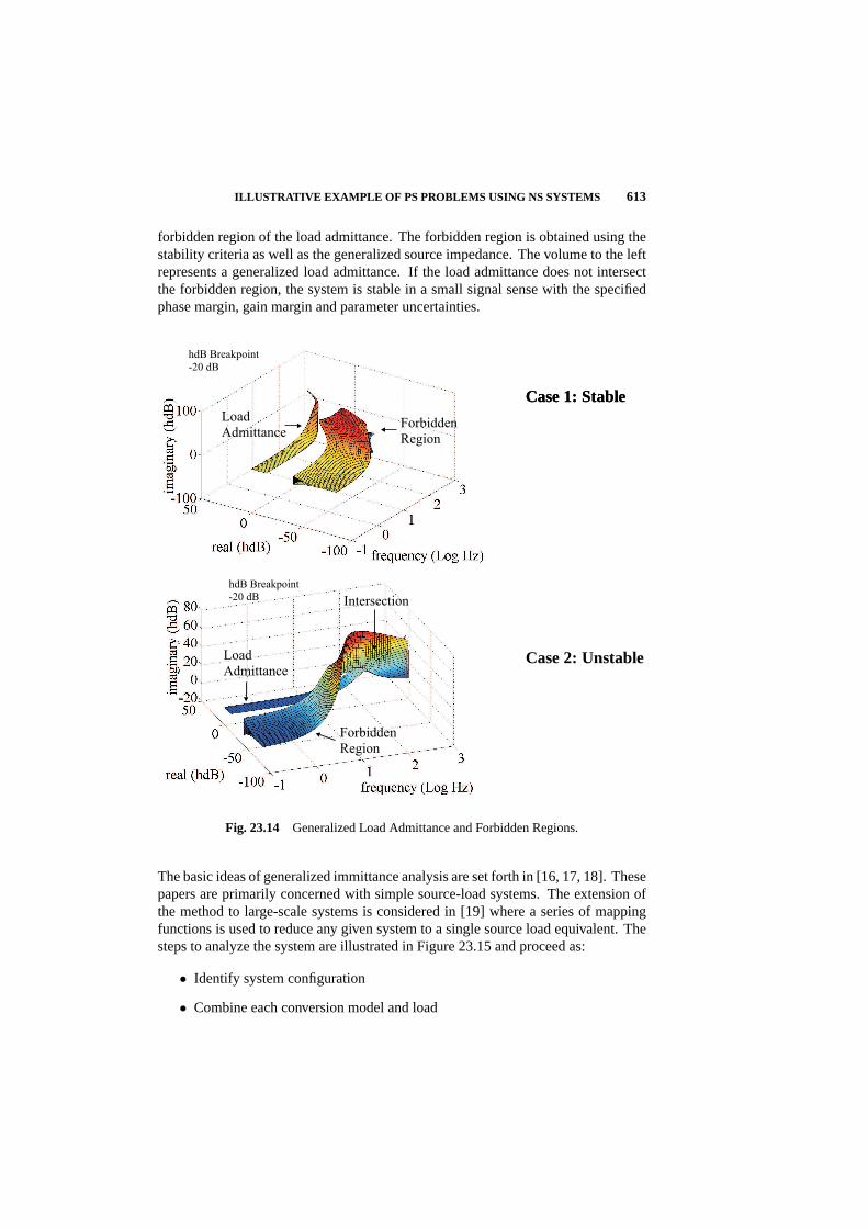
ILLUSTRATIVE EXAMPLE OF PS PROBLEMS USING NS SYSTEMS 613
forbidden region of the load admittance. The forbidden region is obtained using thestability criteria as well as the generalized source impedance. The volume to the leftrepresents a generalized load admittance. If the load admittance does not intersectthe forbidden region, the system is stable in a small signal sense with the specifiedphase margin, gain margin and parameter uncertainties.
Case 1: Stable Case 1: Stable
Case 2: Unstable
Fig. 23.14 Generalized Load Admittance and Forbidden Regions.
The basic ideas of generalized immittance analysis are set forth in [16, 17, 18]. Thesepapers are primarily concerned with simple source-load systems. The extension ofthe method to large-scale systems is considered in [19] where a series of mappingfunctions is used to reduce any given system to a single source load equivalent. Thesteps to analyze the system are illustrated in Figure 23.15 and proceed as:
• Identify system configuration
• Combine each conversion model and load

614 CONTROL, OPTIMIZATION, SECURITY & SELF-HEALING OF BP SYSTEM
• Combine the resulting three parallel aggregate L-converters into a single sourceand a single effective load.
Details on converter types, mapping operations, and intermediate stability tests alongwith more complete examples including other systems are set forth in [19].
(a). Original System.
(b). System after simplification.
(c). Final system.
Fig. 23.15 Immittance Based Reduction Process.
Experimental ValidationOne of the key measures in evaluating these methods is how well they predictmeasured performance. Figure 23.16 and Figure 23.17 depict the measured timedomain performance for Case 1 and Case 2 conditions, respectively. As can seen,the experimental results are consistent with both the time domain simulation andthe Generalized Immittance Analysis. Once again, ADP methods could provideimportant new ways to explore the boundaries of system stability and to extend thetreatment of system nonlinearities.
23.4.4 Stability Analysis Method 3: Polytopic Stability Analysis
In the preceding section, stability analysis of a power electronics based distribu-tion system using time domain simulation and generalized immittance analyses wasdemonstrated, with excellent results. However, there are shortcomings inherent to

ILLUSTRATIVE EXAMPLE OF PS PROBLEMS USING NS SYSTEMS 615
Port bus voltage
Zone 1 voltage (at input to IM)
Zone 2 voltage (at input to MC)
Zone 3 voltage (at input to CPL)
Fig. 23.16 Measured System Performance for Case 1.
Port bus voltage
Zone 1 voltage (at input to IM)
Zone 2 voltage (at input to MC)
Zone 3 voltage (at input to CPL)
Fig. 23.17 Measure System Performance for Case 2.

616 CONTROL, OPTIMIZATION, SECURITY & SELF-HEALING OF BP SYSTEM
either method. In the case of time domain simulation, the results are limited to avery narrow range of conditions. Massive numbers of trajectories must be evaluatedto gain confidence in the system performance. In the case of generalized immittanceanalysis, in some sense a more powerful result is obtained. Using a single analysis, anentire range of operating points can be proven to be locally stable. Furthermore, thisapproach can be used as a design synthesis tool by providing a method to formulatecomponent specifications. However, the generalized immittance design approachdoes not guarantee a bounded response in the presence of large disturbances. Hence,there is motivation to perform a stability analysis in which a system can be proven tohave an appropriately bounded response to large disturbances.
To this end consider a broad class of nonlinear systems modeled by:
x = F(x,u) (23.29)
y = h(x,u) (23.30)
are considered, wherex ∈ <n is the state vector,u ∈ <m is the input vector, andy ∈ <p is the output vector. The above nonlinear model is referred to as the truthmodel of the underlying system. Systems of this form may be analyzed by thedirect method of Lyapunov [10] and [11]. However, there are difficulties associatedwith applying the direct method of Lyapunov including the determination of a validLyapunov function candidate [20]. Analytical means are often impractical if notimpossible so a numerical approach is necessary. Through the use of polytopicmodeling and linear matrix inequalities the search for possible Lyapunov functioncandidates can be automated.
Defining local models of the form:
x = Ax + Bu + φx (23.31)
y = Cx + Du + φy (23.32)
that approximate the behavior of the truth model at a modeling point,(x0,u0),of interest. The particular characteristics that the local model encapsulates variesdepending on the method used in obtaining the local model. Examples include Taylorseries, Teixeira-_Zak [21], and the generalized Teixeira-_Zak base approximations[22]. All three types of models coincide with the truth model at the operating point.In addition, the Teixeira-_Zak based model and the Taylor series based model areproportional and coincide, respectively, to the first order behavior at the operatingpoint.
One characteristic of particular interest, but not enforced by the above approximationmethods, is having the right hand sides of the local model and the truth model equalone another at the equilibrium pair,(xe,ue), and the modeling point. Assigningcoincident equilibrium pairs can be accomplished by the following procedure.
Step one: form the local model at the modeling point of interest. Step two: performa coordinate transformation on the local model shifting the desired equilibrium pair

ILLUSTRATIVE EXAMPLE OF PS PROBLEMS USING NS SYSTEMS 617
to the origin. Step three: perform the generalized Teixeira-_Zak based approximationon the shifted local model. Step four: shift the local model back to the originalcoordinates.
Once the local models have been obtained they are used as ingredients for thepolytopic models constructed using a convex combination of local models:
x =r∑
i=1
wi(θ) [Aix + Biu + φxi] (23.33)
y =r∑
i=1
wi(θ) [Cix + Diu + φyi] (23.34)
Thus, (23.33) and (23.34) consist ofr local models, defined byAi,Bi, φxi, Ci , Di,φyi, combined by weighting functions,Wi. The weighting functions must satisfy
0 ≤ wi(θ) ≤ 1,r∑
i=1
wi(θ) = 1, whereθ may be a function ofx or u. Polytopic
models can accurately represent the nonlinear system over a wide range of operation.Although the truth model already has this property the structure of the polytopicmodel readily lends itself to searching for a Lyapunov function candidate.
Herein it is assumed that all of the local models have coincident equilibrium pairsand the Lyapunov function candidate is of the form:
V = x′Px where x = x− xe (23.35)
Based upon these assumptions the following proposition can be stated.
Proposition 23.4.1 : If there exists a commonP = P ′ > 0 such that,
A′iP + PAi < 0, i = 1, . . . , r (23.36)
then the equilibrium state satisfying:
Aixe + Biue + φi = 0 i = 1, . . . , r (23.37)
is globally uniformly asymptotically stable (GUAS) in the sense of Lyapunov (ISL)[22]. The search for a matrix P can be automated by setting up the system of linearmatrix inequalities of the form (23.36) and using commercially available optimiza-tion routines. If a common P is found the polytopic model is globally uniformlyasymptotically stable in the sense of Lyapunov. However stability analysis of thetruth model is incomplete.
To complete the stability analysis of the truth model it is necessary to find the regionof attraction around the equilibrium state using the direct method of Lyapunov. Theregion of attraction can be approximated by the largest level set of (23.35) containedwithin the region defined byV < 0, where:
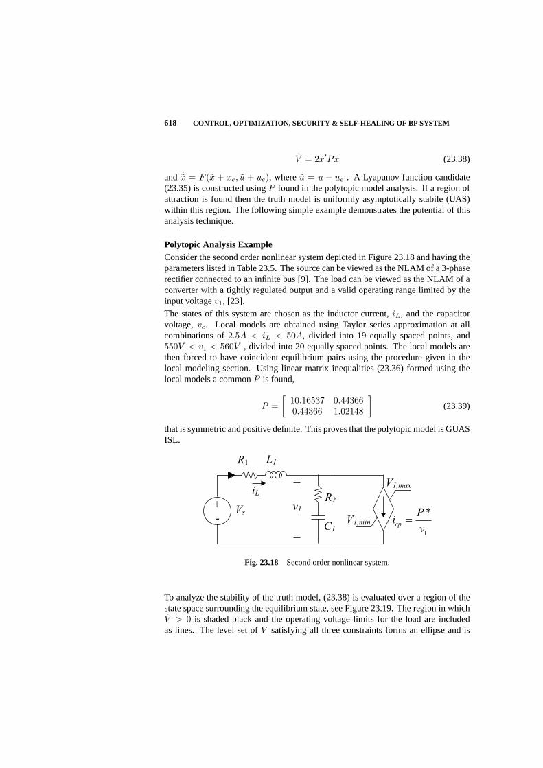
618 CONTROL, OPTIMIZATION, SECURITY & SELF-HEALING OF BP SYSTEM
V = 2x′P˙x (23.38)
and ˙x = F (x + xe, u + ue), whereu = u − ue . A Lyapunov function candidate(23.35) is constructed usingP found in the polytopic model analysis. If a region ofattraction is found then the truth model is uniformly asymptotically stabile (UAS)within this region. The following simple example demonstrates the potential of thisanalysis technique.
Polytopic Analysis ExampleConsider the second order nonlinear system depicted in Figure 23.18 and having theparameters listed in Table 23.5. The source can be viewed as the NLAM of a 3-phaserectifier connected to an infinite bus [9]. The load can be viewed as the NLAM of aconverter with a tightly regulated output and a valid operating range limited by theinput voltagev1, [23].
The states of this system are chosen as the inductor current,iL, and the capacitorvoltage,vc. Local models are obtained using Taylor series approximation at allcombinations of2.5A < iL < 50A, divided into 19 equally spaced points, and550V < v1 < 560V , divided into 20 equally spaced points. The local models arethen forced to have coincident equilibrium pairs using the procedure given in thelocal modeling section. Using linear matrix inequalities (23.36) formed using thelocal models a commonP is found,
P =[
10.16537 0.443660.44366 1.02148
](23.39)
that is symmetric and positive definite. This proves that the polytopic model is GUASISL.
Fig. 23.18 Second order nonlinear system.
To analyze the stability of the truth model, (23.38) is evaluated over a region of thestate space surrounding the equilibrium state, see Figure 23.19. The region in whichV > 0 is shaded black and the operating voltage limits for the load are includedas lines. The level set ofV satisfying all three constraints forms an ellipse and is

ILLUSTRATIVE EXAMPLE OF PS PROBLEMS USING NS SYSTEMS 619
Vs 595.49 V C1 1.051 mF
R1 0.526 Ω P* 10 kW
L1 11.32 mH V1min 550 V
R2 0.08305 Ω V1max 650 V
Table 23.5 Second order nonlinear system parameters.
included along with one trajectory of the truth model. The ellipse identifies a regionof uniform asymptotic stability for the truth model. The trajectory demonstrates theconservative nature of the Lyapunov based analysis.
23.4.5 Remarks on the Three Stability Analysis Methods
Each of the three stability analysis methods presented above contain serious limita-tions for which ADP methods may provide fundamental improvements. A discussionof these limitations and potential improvements follow. Actual stability involves thebehavior of the time evolution of the system state trajectory. As discussed in theDC Stability Definition section, the determinations of the boundary between stableand unstable operation is difficult and dependent on a specific, formal definition ofstability. A more useful metric would involve the calculation of a stability marginwhich might be a generalization of the classic Nyquist gain and phase margins.
The difficulty in experimental stability observations involves the need to performexhaustive and potentially destructive testing; ambiguity regarding the specific onsetof instability; and problems isolating the source of instability due to the dynamicallyinterdependent nature of power systems. Compared to experimental observation,time domain simulation lessens the burden of time domain stability assessment. Un-fortunately, exhaustive time domain simulation remains computationally prohibitive.Moreover, ambiguities regarding the source and onset of instability remain. ADPmethods could provide fundamentally new time domain methods to detect the prox-imity to instability and avoid unstable modes of operation.
Frequency domain generalized immittance stability assessment provides an experi-mentally validated unambiguous stability assessment including stability margins butis limited to systems represented by linear networks or equivalently, small perturba-tions of a linear approximation of the actual system. The use of ADP methods toextend generalized immittance analysis to uncertain, stochastic and nonlinear systemscould have a profound effect on the design of isolated DC power systems.
While time domain observation and immittance based analysis both offer insight intothe stability of nonlinear systems Lyapunov methods identify a region of asymptotic

620 CONTROL, OPTIMIZATION, SECURITY & SELF-HEALING OF BP SYSTEM
Fig. 23.19 V evaluated over the state space.
stability about an equilibrium point. The traditional obstacles to nonlinear Lyapunovstability assessment include the search for Lyapunov function candidates and overlyconservative results. Recently, a polytopic model structure has been shown whichallows automation of the search for function candidates. Figure 23.19 provides anillustrative example of a stable state trajectory derived from polytopic Lyapunov sta-bility analysis of the Navy IPS benchmark system. Although ADP methods could beapplied to the generation of polytopic models, a more direct and profound opportunityinvolves using ADP to search for the least conservative Lyapunov function candidate.The ultimate objective involves the "holy grail" of system stability: the determinationof the region of asymptotic stability for higher order nonlinear systems.
23.5 SUMMARY OF POWER SYSTEM CHALLENGES AND TOPICS
The previous sections have provided some detailed discussions of several importantpower systems problems illustrated by two important systems: the terrestrial andthe Navy systems, respectively. In the present section, we would like to providea comprehensive summary of what is needed in power systems applications withindividual topics identified and discussed.
23.5.1 Transmission Stability Analysis
Much of the non-linear analysis of power system behavior subjected to exogenousdisturbances has focused on conventional analytical methods including risk assess-
SUMMARY OF POWER SYSTEM CHALLENGES AND TOPICS 621
ment and Lyapunov stability assessment. Voltage and angle stability assessments areneeded to ensure dynamic reconfiguration in response to system faults and distur-bances. Since the margin of stability cannot be obtained using numerical methods,an energy-based method has been proposed for angle stability. To date, real-timeevaluation of the system under different loading and unknown contingencies has notbeen implemented.
Several researchers in the US and abroad have done extensive research on the ap-plication of the Newton-Raphson method, which accurately shifts a set of electricalnetwork poles and transfer function zeros to more suitable location in the complexplane to improve the harmonic voltage performance of the power system. Theirwork dealt with eigenvalue sensitivity coefficients, which are used for computingthe element changes that are the most cost effective in computing the system Jaco-bian elements for the Newton’s method. Realistic results of a modeled system showpromising results [29]
Also work on small signal stability, control applications and harmonic analysis havebeen undertaken recently by researchers in determining Hopf bifurcations and mini-mum distances to small signal stability boundaries in the control parameter space aswell as computation of reduced models of high order multivariable transfer functions[30, 31].
23.5.2 Voltage Stability
Voltage stability employs chaos and bifurcation theory to solve the differential equa-tions and assess the stable and unstable equilibrium points (SEP) and (UEP), respec-tively. The technique based on load flow requires a series of load flow runs withchanges in parameter space (load) and category.
Solution
Traditional methods for solving stability problems include Proximity Indicator method,Singular Value Decomposition, Jacobian Condition Number and Energy Marginmethods. To achieve a high performance method of voltage stability, the followingchallenges need to be addressed: (1) Increased nonlinearity of the problem space and(2) Model and parameter uncertainty. For theses challenges, adaptive control andoptimization techniques are needed in solving the uncertainty problem inherent indata measurements to enhance system self-healing under any contingency.
23.5.3 Adaptive Control and Optimization
Adaptation and control strategy scheduling must consider the stochastic and dynami-cally interdependent attributes of power systems. An efficient optimization techniquemust:
• Achieve optimal scheduling subject to technical constraints,
622 CONTROL, OPTIMIZATION, SECURITY & SELF-HEALING OF BP SYSTEM
• Adapt to perturbation of power system dynamics due over time (in state, Pareto,controls),
• Adapt to varying random noise and uncertainties,
• Adapt to changes in system structure, and, finally,
• Distinguish between observable and unobservable measurements.
The techniques available to handle these problems are based on vague methods andsomewhat heuristic methods that tend to give a non-optimal solution. The systemstochasticity and dynamic interdependence lead to unstable, non-feasible and non-optimal solutions.
Solution:
Using Dynamic Stochastic Optimal Power Flow (DSOPF), we need a multi-objectivescheme to accommodate evolving systems dynamics in the presence of missing orcorrupted measurements. State-of-the-art techniques from Operations Research,Information Technology and Computational Intelligence communities can improveexisting optimization methods.
23.5.4 Reliability Assessment
One of the increasing requirements of Electric Power Systems (EPS) and IntegratedPower Systems (IPS) is their ability to survive under different attacks and maintainsome level of invulnerability. The assessment of indices such as Loss of Load Prob-ability (LOLP) and Expected Unserved Energy (EUE) is aimed at the determinationof what energy / load can be supplied over time for different reliability services. Thecost component balances the cost of reliability improvements with the cost of servicedisruptions. The ultimate goal is to achieve the maximum reliability under a varietyof probable contingencies.
The complexity associated with reliability improvement may significantly increasethe cost of service delivery. As a result, cost effective reliability and reconfigu-ration assessment strategies are needed that address the following challenges: (1)Non-linearity of the power system parameters (2) Uncertainty in load demand andgeneration availability (3) System dynamics and (4) Stochasticity of the system pa-rameters.
Intelligent control methods including Adaptive Critics Designs, Fuzzy Logic andArtificial Neural Networks (ANN) methods may provide adaptive stochastic solutionsto the general problem formulation.
23.5.5 Economic Benefit and Control Strategy
Innovative control and optimization strategies for improving power systems efficiencyand security are urgently required. Moreover, the overall nonrecurring and recurring

SUMMARY OF POWER SYSTEM CHALLENGES AND TOPICS 623
personnel, equipment and software costs must be calculated. These infrastructurecosts must be balanced by the economic and social impacts and the value of improvedcontinuity of power delivery. Table 23.6 presents a summary of the terrestrial powersystem economic benefits and control strategy tradeoffs.
Power System Economic Benefit and Control Strategy Objectives
System Requirements
Summary of
Terrestrial
Reference
Problems Existing Future
New Optimization
Techniques
Voltage
Stability
Static model with
limited dynamics
Dynamically
interdependent system
with uncertainty
Voltage stability margin
(VSM) constraints using
ADP1 DSOPF
2 stochastic
formulation
Angle
Stability
Transient model
with limited
dynamics
Dynamically
interdependent online
stochastic assessment
and control
Constrained angle stability
margin (ASM) using ADP
DSOPF subject to
contingencies
CongestionProbability based
static congestion
constraints
Dynamically
interdependent
congestion based
stochastic constraints
Dynamic margin based
index for congestion
subject to contingencies
and available transfer
capability
Reliability
Expected Unserved
Energy (EUE ) and
Loss of Load
Probability, (LOLP)
Dynamically
interdependent margins
subject to stochastic
contingencies
Time domain continuity of
service ADP DSOPF
formulation
Coordinated
Control
Model is either
discrete or
continuous
Dynamically
interdependent hybrid
modeling of discrete
and continuous
processes
Hybrid adaptive
distributed control with
contingency management
Unit
Commitment,
Optimal Power
flow
Lagrange relaxation
methods
Dynamically
interdependent
planning subject to
stochastic
contingencies
Dynamic and stochastic
indices based on ADP and
Interior Point (IP) Methods
DSOPF
Cost Benefit
Analysis
Net Present Value
(NPV) and Annual
Worth or Cost
(AW/AC)
Incorporation of
uncertainty into market
and investment and
predictions
Stochastic ADP
DSOPF formulation
1Approximate Dynamic Programming (ADP)
2Dynamic Stochastic Optimal Power
Flow
Table 23.6 Power System Economic Benefit and Control Strategy.
Cost benefit analysis should include consideration of nonlinear system dynamics,hierarchical control law implementation, optimal algorithms and intelligent technolo-gies to achieve the desired stability and reliability. Intelligent control solutions suchas Artificial Neural Networks, Learning Algorithms, and Fuzzy Logic approachesmay provide hybridized methods which extend existing tools.

624 CONTROL, OPTIMIZATION, SECURITY & SELF-HEALING OF BP SYSTEM
To this end, we present a number of control / optimization problems as challengesto researchers wishing to explore new algorithms and determine quantifiable perfor-mance metrics. Problems associated with realistic control / optimization solutionsinclude: (1) Incomplete system knowledge/model formulation and data, (2) Nonlin-earities, (3) Noise, and (4) Un-modeled system dynamics and delays.
23.5.6 Isolated System Stability
The Navy benchmark system represents the characteristics of emerging isolatedpower systems including a variety of vehicle and alternative energy applications.These systems differ from conventional terrestrial systems in that they involve (1)finite intertia sources, (2) power electronic-based distribution and conversion, (3)loads and disturbancesthat are large relative to the source capacity and (4) constantpower loads with potentially destabilizing system dynamics. Due to the high costand potentially catastrophic consequences of interruption of power delivery to criticalpower services, the Navy benchmark problem focuses on nonlinear system stabilitydespite stochastic model variations and disruptions. The key opportunity involvesthe use of ADP methods to improve power system robustness with respect to naturaland hostile disruptions. One approach involves new methods to more accuratelydetermine system stability boundaries. Improved nonlinear stochastic stability pre-dictions would have important offline design applications, along with the potential toprovide online stability margin assessments. The second approach involves the useof ADP to derive intrinsically nonlinear stabilizing controllers with improved qualityand continuity of service.
23.6 SUMMARY
This chapter presents a grand overview and introductory remarks for power systembenchmark of both utility and Navy systems. Details of existing modeling techniquesfor such systems have been presented and their limitations addressed.
Conventional optimization and control system theories and tools have been used insolving the power system problems of both utility and Navy systems. However,since the computational tools developed by power system researchers are limitedin some extent to dealing with uncertainties of the power system along with itsmultifaceted dynamics, new optimization techniques that can handle uncertaintiesand with enhanced capability for predicting future performances are required.
The formulation of different power system problems such as the modeling of systemcomponents with dynamics, design and analysis as well as control coordination arepresented with illustrative examples using conventional techniques. Test cases ofestablished work have been added to supplement readers understanding.
The basic idea is to extend the performance of these conventional tools by incorpo-rating new computational intelligence approaches, which can handle foresight anduncertainty of the power grid. Approximate Dynamic Programming (ADP), a pow-

SUMMARY 625
erful tool from the computational intelligence community, is capable of handlingthese problems. Various power system problems are reformulated such that ADP canhandle it effectively.
Bibliography
1. Architectures for Secure and Robust Distributed Infrastructures,University Re-search Initiative Web Sitehttp://element.stanford.edu/ lall/projects/architectures/.
2. James A. Momoh,Electric Power System Applications of Optimization,MarcelDekker Inc. New York, U.S.A. 2001.
3. A.A. Fouad and Vijay Vittal,Power Systems Transient Stability Analysis Usingthe Transient Energy Function Method,Prentice Hall, Cliffs, New Jersey, 1992.
4. James A. Momoh and Mohamed El-Hawary,Electric Systems Dynamics andStability with Artificial Intelligence Applications,Marcel Dekker Inc. New York,U.S.A. 2000.
5. Pekarek et. al., “A Hardware Power Electronic-Based Distribution and PropulsionTestbed,”Sixth IASTED International Multi-Conference On Power and EnergySystem,Marina del Rey, California, May 12-15, 2002.
6. S.D. Sudhoff, S.D. Pekarek, B.T. Kuhn, S.F. Glover, J. Sauer, D.E. Delisle,“Naval Combat Survivability Testbeds for Investigation of Issues in ShipboardPower Electronics Based Power and Propulsion Systems,”Proceedings of theIEEE Power Engineering Society Summer Meeting,Chicago, Illinois, July 21-25,2002.
7. S.D. Pekarek et. al., “Development of a Testbed for Design and Evaluation ofPower Electronic Based Generation and Distribution System,”SAE2002 PowerSystems Conference,Coral Springs, Florida, October 29-31, 2002.
8. S.D. Sudhoff, S.F. Glover, S.H. Zak, S.D. Pekarek, E.L Zivi, D.E. Delisle, D.Clayton, “Stability Analysis Methodologies For Dc Power Distribution Systems,”Proceedings of the Thirteenth Ship Control Systems Symposium (SCSS 2003),Orlando, Florida, April 7-9, 2003.
9. P.C. Krause, O. Wasynczuk, S.D. Sudhoff,Analysis of Electric Machinery, 2ndEd.,John Wiley & Sons, Inc., New York, 2002.
10. S.H. Zak,Systems and Control,Oxford University Press, New York, 2003.
626

BIBLIOGRAPHY 627
11. H.K. Khalil, Nonlinear Systems, 2nd Ed.,Prentice Hall, Upper Saddle River,New Jersey, 1996.
12. www.ESAC.info.
13. S.D. Pekarek, S.D. Sudhoff, J.D. Sauer, D.E.Delisle, E.L. Zivi, “Overview ofthe Naval Combat Survivability Program,”Proceedings of the Thirteenth ShipControl Systems Symposium (SCSS 2003),Orlando, Florida, April 7-9, 2003.
14. MATLAB The Language of Technical Computing,MATLAB The Language ofTechnical Computing, The MathWorks, Inc., 3 Apple Hill Drive, Natick, MApp. 01760-2098, 2000.
15. Advanced Continuous Simulation Language (ACSL) Reference Manual,AegisSimulation, Inc., 6703 Odyssey Drive, Suite 103, Huntsville, AL, 35806, 1999.
16. S.D. Sudhoff, D.H. Schmucker, R.A. Youngs, H. J. Hegner, “Stability Analysisof DC Distribution Systems Using Admittance Space Constraints,”Proceedingsof The Institute of Marine Engineers All Electric Ship 98,London, September29-30, 1998.
17. S.D. Sudhoff, S.F. Glover, “Three Dimensional Stability Analysis of DC PowerElectronics Based Systems,”Proceedings of the Power Electronics SpecialistConference,Galway, Ireland, pp. 101-106, June 19-22, 2000 .
18. S.D. Sudhoff, S.F. Glover, P.T. Lamm, D.H. Schmucker, D.E. Delisle, “Admit-tance Space Stability Analysis of Power Electronic Systems,”IEEE Transactionson Aerospace and Electronics Systems,vol. 36. no. 3, pp. 965-973, July 2000.
19. S.D. Sudhoff, S.D. Pekarek, S.F. Glover, S.H. Zak, E. Zivi, J.D. Sauer, D.EDelisle, “Stability Analysis of a DC Power Electronics Based Distribution Sys-tem,” SAE2002 Power Systems Conference,Coral Springs, Florida, October29-31, 2002.
20. H. Lim, D.C. Hamill, “Problems of computing Lyapunov exponents in powerelectronics,”Proceedings of the IEEE International Symposium on Circuits andSystems,pp. 297-301, May, 1999.
21. M.C.M Teixeira, S.H. Zak, “Stabilizing controller design for uncertain nonlinearsystems using fuzzy models,”IEEE Transactions on Fuzzy Systems,vol. 7(2),pp. 133-142, April 1999.
22. S.F. Glover, S.H. zak, S.D. Sudhoff, and E.J. Zivi, “Polytopic modeling andLyapunov stability analysis of power electronics systems,”Society of AutomotiveEngineers 2002 Power Systems Conference,Coral Springs, Florida, October 29-31, 2002.
23. S.D. Sudhoff, K.A. Corzine, S.F. Glover, H.J. Hegner, H.N. Robey, “ DC link sta-bilized field oriented control of electric propulsion systems,”IEEE Transactionson Energy Conversion,vol. 13(1),pp. 27-33, March 1998.
628 BIBLIOGRAPHY
24. A. A. Fouad and Vijay Vittal, “Power Systems Transient Stability AnalysisUsing the Transient Energy Function Method,”Control and Dynamic Systems(C.T. Leonides, ed.),Academic Press, San Diego, CA, 1991.
25. Allen J. Woods and Bruce F. Wollenberg,Power Generation, Operation andControl,John Wiley & Sons, Inc., New York, 1984.
26. James A. Momoh and Mohamed El-Hawary,Electric Systems, Dynamics, andStability with Artificial Intelligence Application,Marcel Dekker Inc., New York,U.S.A., 2000.
27. Gerald T. Heydt,Computer Analysis Methods in Power Systems,MacmillanPublishing Co., New York, 1986.
28. Arthur R. Bergen,Power Systems Analysis,Prentice-Hall, Inc., EnglewoodCliffs, NJ, 1986.
29. Sergio Luis, Nelson Martins and Leonardo Tadeu Garcia Lima, “A Newton-Raphson Method based on Eigenvalues Sensitivities to improve harmonic VoltagePerformance,”IEEE Transactions on Power Delivery,vol. 18, No. 1, January2003.
30. Nelson Martins, S. Gomes Jr, Paulo E.M. Quintao, J.C.R. Ferraz, S.L Varricchioand A. de Castro, “Some Recent Developments in Small Signal Stability andControl,” Power Engineering Society Winter Meeting,vol. 2, pp. 1171-1177,27-31 Jan. 2002.
31. Ajjarapu, V., “Application of bifurcation and continuation methods for the anal-ysis of power system dynamics,”Proceedings of the 4th IEEE Conference onControl Applications,pp. 52 -56, 1995.


