Scan Detection: A Data Mining Approach Gy¨ orgy J. Simon Computer Science Univ. of Minnesota [email protected]Hui Xiong MSIS Dept. Rutgers Univ. [email protected]Eric Eilertson Computer Science Univ. of Minnesota [email protected]Vipin Kumar Computer Science Univ. of Minnesota [email protected]Abstract A precursor to many attacks on networks is often a reconnaissance operation, more commonly referred to as a scan. Despite the vast amount of attention focused on methods for scan detection, the state-of- the-art methods suffer from high rate of false alarms and low rate of scan detection. In this paper, we formalize the problem of scan detection as a data mining problem. We show how the network traffic data sets can be converted into a data set that is appropriate for running off-the-shelf classifiers on. Our method successfully demonstrates that data mining models can encapsulate expert knowledge to create an adaptable algorithm that can substantially outperform state-of- the-art methods for scan detection in both coverage and precision. 1 Introduction A precursor to many attacks on networks is often a reconnaissance operation, more commonly referred to as a scan. Identifying what attackers are scanning for can alert a system administrator or security analyst to what services or types of computers are being targeted. Knowing what services are being targeted before an at- tack allows an administrator to take preventative mea- sures to protect the resources e.g. installing patches, firewalling services from the outside, or removing ser- vices on machines which do not need to be running them. Given its importance, the problem of scan detection has been given a lot of attention by a large number of researchers in the network security community. Initial solutions simply counted the number of destination IPs that a source IP made connection attempts to on each destination port and declared every source IP a scanner whose count exceeded a threshold [16]. Many enhancements have been proposed [18, 5, 15, 9, 14, 13], but despite the vast amount of expert knowledge spent on these methods, current, state-of-the-art solutions still suffer from high percentage of false alarms or low ratio of scan detection. For example, a recently developed scheme by Jung [5] has better performance than earlier methods, but it requires that scanners attempt connections to several hosts on a destination port before they can be detected. This constraint limits the scheme’s applicability because a sizable portion of the scanners attempt connections to only one host on each port in a typical observation window giving a net result of poor coverage. Data mining techniques have been successfully applied to the generic network intrusion detection problem[8, 2, 10], but not to scan detection. 1 In this pa- per, we present a method for transforming network traf- fic data into a feature space that successfully encodes the accumulated expert knowledge. We show that an off-the-shelf classifier, Ripper[3], can achieve outstand- ing performance both in terms of missing only very few scanners and also in terms of very low false alarm rate. While the rules generated by Ripper make perfect sense from the domain perspective, it would be very difficult for a human analyst to invent them from scratch. 1.1 Contributions This paper has the following key contributions: • We formalize the problem of scan detection as a data mining problem and present a method for transforming network traffic data into a data set that classifiers are directly applicable to. Specif- ically, we formulate a set of features that encode expert knowledge relevant to scan detection. • We construct carefully labeled data sets to be used for training and test from real network traffic data at the University of Minnesota and demonstrate that Ripper can build a high-quality predictive model for scan detection. We show that our method is capable of very early detection (as early as 1 Scans were part of the set of attacks used in the KDD Cup ’99 [1] data set generated from the DARPA ’98/’99 data sets. Nearly all of these scans were of the obvious kind that could be detected by the simplest threshold-based schemes that simply look at the number of hosts touched in a period of time or connection window. 118
A precursor to many attacks on networks is oftena reconnaissance operation, more commonly referredto as a scan. Despite the vast amount of attentionfocused on methods for scan detection, the state-of-the-art methods suffer from high rate of false alarmsand low rate of scan detection. In this paper, weformalize the problem of scan detection as a data miningproblem. We show how the network traffic data setscan be converted into a data set that is appropriatefor running off-the-shelf classifiers on. Our methodsuccessfully demonstrates that data mining models canencapsulate expert knowledge to create an adaptablealgorithm that can substantially outperform state-of-the-art methods for scan detection in both coverage andprecision.
1 Introduction
A precursor to many attacks on networks is often areconnaissance operation, more commonly referred toas a scan. Identifying what attackers are scanning forcan alert a system administrator or security analyst towhat services or types of computers are being targeted.Knowing what services are being targeted before an at-tack allows an administrator to take preventative mea-sures to protect the resources e.g. installing patches,firewalling services from the outside, or removing ser-vices on machines which do not need to be runningthem.
Given its importance, the problem of scan detectionhas been given a lot of attention by a large number ofresearchers in the network security community. Initialsolutions simply counted the number of destinationIPs that a source IP made connection attempts to oneach destination port and declared every source IP ascanner whose count exceeded a threshold [16]. Manyenhancements have been proposed [18, 5, 15, 9, 14, 13],but despite the vast amount of expert knowledge spenton these methods, current, state-of-the-art solutionsstill suffer from high percentage of false alarms or lowratio of scan detection.
For example, a recently developed scheme by Jung[5] has better performance than earlier methods, but itrequires that scanners attempt connections to severalhosts on a destination port before they can be detected.This constraint limits the scheme’s applicability becausea sizable portion of the scanners attempt connectionsto only one host on each port in a typical observationwindow giving a net result of poor coverage.
Data mining techniques have been successfullyapplied to the generic network intrusion detectionproblem[8, 2, 10], but not to scan detection.1In this pa-per, we present a method for transforming network traf-fic data into a feature space that successfully encodesthe accumulated expert knowledge. We show that anoff-the-shelf classifier, Ripper[3], can achieve outstand-ing performance both in terms of missing only very fewscanners and also in terms of very low false alarm rate.While the rules generated by Ripper make perfect sensefrom the domain perspective, it would be very difficultfor a human analyst to invent them from scratch.
1.1 Contributions This paper has the following keycontributions:
• We formalize the problem of scan detection as adata mining problem and present a method fortransforming network traffic data into a data setthat classifiers are directly applicable to. Specif-ically, we formulate a set of features that encodeexpert knowledge relevant to scan detection.
• We construct carefully labeled data sets to be usedfor training and test from real network traffic dataat the University of Minnesota and demonstratethat Ripper can build a high-quality predictivemodel for scan detection. We show that our methodis capable of very early detection (as early as
1Scans were part of the set of attacks used in the KDD Cup ’99
[1] data set generated from the DARPA ’98/’99 data sets. Nearly
all of these scans were of the obvious kind that could be detected
by the simplest threshold-based schemes that simply look at thenumber of hosts touched in a period of time or connection window.
118
the first connection attempt on the specific port)without significantly compromising the precision ofthe detection.
• We present extensive experiments on real-worldnetwork traffic data. The results show that theproposed method has substantially better perfor-mance than the state-of-the-art methods both interms of coverage and precision.
2 Background and Related Works
Until recently, scan detection has been thought of asthe process of counting the distinct destination IPstalked to by each source on a given port in a certaintime window [16]. This approach is straightforward toevade by decreasing the frequency of scanning. Witha sufficiently low threshold (to allow capturing slowscanners), the false alarm rate can become high enoughto render the algorithm useless. On the other hand,higher thresholds can leave slow and stealthy scannersundetected. A number of more sophisticated methods[9, 18, 15, 5, 4] have been developed to address thelimitations of the basic method.
Robertson [15] assigns an anomaly score to a sourceIP based on the number of failed connection attempts ithas made. This scheme is more accurate than the onesthat simply count all connections since scanners tendto make failed connections more frequently. However,the scanning results still vary greatly depending on thedefinition of a failed connection and how the thresholdis set. Lickie [9] uses a statistical approach to determinethe likelihood of a connection being normal versus beingpart of a scan. The main flaw of this algorithm isthat it generates too many false alarms when accessprobabilities are highly skewed (which is often the case.)SPICE [18] is another statistical-anomaly based systemwhich sums the negative log-likelihood of destinationIP/port pairs until it reaches a given threshold. Oneof the main problems with this approach is that it willdeclare a connection to be a scan simply because it isto a destination that is infrequently accessed.
The intuition behind SPICE is partly correct. Itis true that destinations that are accessed only byscanners are rare, but the converse is not true. A schemeproposed by Ertoz et al. [4] assigns a scan score to eachsource IP on each destination. If the requested serviceis offered – regardless of how infrequently it is used –the score is not increased. If the requested service doesnot exist, the score is increased by the reciprocal of thelog frequency of the destination. This scheme achievesfairly good performance, and is generally comparable tothe TRW scheme in precision and recall that we describenext.
The current state-of-the-art for scan detection isThreshold Random Walk (TRW) proposed by Jung etal. [5]. It traces the source’s connection history per-forming sequential hypothesis testing. The hypothesistesting is continued until enough evidence is gathered todeclare the source either scanner or normal. Assumingthat the source touched k distinct hosts, the test statis-tics (the likelihood ratio of the source being scanner ornormal) is computed as follows:
Λ =
k∏
i=1
γ0 if the first connection tohost i fails
1
γ1
otherwise,
where γ0 and γ1 are constants. The source is declared ascanner, if Λ is greater than an upper threshold; normal,if Λ is less than a lower threshold. The thresholdsare computed from the nominal significance level of thetests.
It is worth pointing out that in a logarithmic space,when log γ0 = 1, then log Λ is increased by one everytime a first connection fails and is decreased by oneevery time a first connection succeeds. The threshold inthis logarithmic space (the log of the threshold in theoriginal space) is number of consecutive first-connectionfailures required for a source to be declared a scanner.For simplicity, in the rest of the paper, when we saythreshold, we will refer to the log-threshold.
The authors of TRW recommend using a thresholdof 4 (that is TRW is going to declared an IP scanneronly after having made at least 4 observations). At thisthreshold, TRW can achieve high precision. Reducingthe threshold to 1 will result in an unacceptably highrate of false alarms rendering TRW unable to reliablydetect scans that only make one connection attemptwithin the observation period.
These false alarms are primarily caused by P2Pand backscatter traffic. In recent years when thelegality of certain uses of file sharing networks (basedon P2P) has been questioned in the courtrooms, P2Pnetworks started increasingly utilizing random portsto avoid detection. Peers agree upon a (practically)randomly chosen destination port that they conducttheir communications on. They also maintain a listof the <IP address, destination port> pairs of theirpeers. Upon trying to re-connect to a P2P network,the host makes connection attempts to the hosts on itslist of peers. The hosts on the list may not offer theservice any more – e.g. they may be turned off or theirdynamic IP address changed. To a scan detector, a P2Phost unsuccessfully trying to to connect to its peers mayappear as a scan [7, 6].
Backscatter traffic is another type of network trafficthat can be easily mistaken for scan. Backscatter
119
traffic typically originates from a server under denial-of-service (DoS) attack. In the course of a DoS attack,attackers send a server (the victim) such a large amountof network packets that the server becomes unable torender its usual service to its legitimate clients. Theattackers also falsify the source IP and source port fieldsin these packets, so when the server responds,it sendsits replies to the falsified (random) addresses. For asufficiently large network, there can be enough falsifiedaddresses that fall within the network space, such thatreplies from the victim will make it seem like a scanner:the victim is unsolicitedly sending packets to hosts thatmay not even exist [11].
3 Definitions and Method Description
In the course of scanning, the attacker aims to map theservices offered by the target network. There are twogeneral types of scans (1) horizontal scans, where theattacker has an exploit at his disposal and aims to findhosts that are exploitable by checking many hosts fora small set of services; and (2) vertical scan, wherethe attacker is interested in compromising a specificcomputer or a small set of specific computers. Theyoften scan for dozens or hundreds of services.
Source IP, destination port pairs (SIDPs) are thebasic units of scan detection; they are the potentialscanners. Assume that a user is browsing the Web (des-tination port 80) from a computer with a source IP S.Further assume that S is infected and is simultaneouslyscanning for port 445. Our definition of a scanner allowsus to correctly distinguish between the user surfing theWeb (whose SIDP < S, 80 > is not a scanner) from theSIDP < S, 445 > which is scanning.
Scan Detection Problem Given a set of networktraffic records (network traces) each containing the fol-lowing information about a session (source IP, sourceport, destination IP, destination port, protocol, num-ber of bytes and packets exchanged and whether thedestination port was blocked), scan detection is a clas-sification problem in which each SIDP, whose sourceIP is outside the network being observed, is labeled asscanner if it was found scanning or non-scanner oth-erwise.
Overview of the Solution The essence of ourproposed method is the assumption that given a prop-erly labeled training data set and the right set offeatures, data mining methods can be used to builda predictive model to classify SIDPs (as scanner ornon-scanner).
In case of the scan detection problem, we will ob-serve SIDPs over as long a time period as our computa-tional resources allow and label them with high preci-
sion2. We will train a classifier – any off-the-shelf classi-fier – on this precisely labeled data and let the classifierlearn the patterns characteristic of scanning behavior.Then we can apply this classifier to unlabeled data col-lected over a much shorter observation period and (aswe will demonstrate later) successfully detect scanners.
The success of this method depends on (1) whetherwe can label the data accurately and (2) whether wehave derived the right set of features that facilitatethe extraction of knowledge. Section 3.1 and 3.2 willelaborate on these points.
Choice of classifier. Although most classifiers areapplicable to our problem, some classifiers are bettersuited than others.
Our understanding of data mining classifier algo-rithms guided us towards choosing Ripper. We choseRipper, because (a) the data is not linearly separable,(b) most of the attributes are continuous, (c) the datahas multiple modes and (d) the data has unbalancedclass distribution. Ripper can handle all of these prop-erties quite well. Furthermore, it produces a relativelyeasily interpretable model in the form of rules allow-ing us to assess whether the model reflects reality wellor if it is merely coincidental. An additional benefitis that classification is computationally inexpensive 3.The drawback of Ripper is its greedy optimization al-gorithm and its tendency to overfit the training data attimes. These drawbacks did not set us back too much;we encountered the overfit problem with visible effectonly on one occasion.
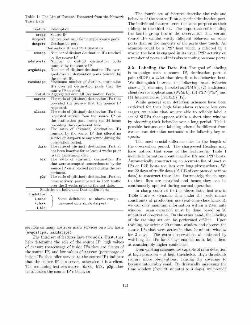
3.1 Features The key challenge in designing a datamining method for a concrete application is the neces-sity to integrate the expert knowledge into the method.A part of the knowledge integration is the derivation ofthe appropriate features. Table 1 provides the list offeatures that we derived.
The first set of features (srcip, scrport,
dstport) serve to identify a record; these features arenot used for classification.
The second set of features contains statistics aboutthe destination IPs and ports. These features provide anoverall picture of the services and hosts involved in thesource IP’s communication patterns. The first feature inthis group, ndstips, is the revered heuristic that definedearly scan detection schemes. In addition, we providefeatures to show whether the source IP was using a few
2As we will explain in Section 3.2, despite our claims about the
poor performance of the current scan detection schemes, labelingat a very high precision is possible under certain circumstances.
3Building the model is computationally expensive, but it canbe performed off-line. It is the actual classification that needs to
be carried out in real-time.
120
Table 1: The List of Features Extracted from the NetworkTrace Data
Feature Description
srcip Source IPsrcport Source port or 0 for multiple source portsdstport Destination port
Destination IP and Port Statistics
ndstip Number of distinct destination IPs touchedby the source IP
ndstports Number of distinct destination portstouched by the source IP
avgdstips Number of distinct destination IPs aver-aged over all destination ports touched bythe source IP.
maxdstips Maximum number of distinct destinationIPs over all destination ports that thesource IP touched.
Statistics Aggregated over All Destination Ports
server The ratio of (distinct) destination IPs thatprovided the service that the source IPrequested.
client The ratio of (distinct) destination IPs thatrequested service from the source IP onthe destination port during the 24 hourspreceding the experiment time.
nosrv The ratio of (distinct) destination IPstouched by the source IP that offered noservice on dstport to any source during theobservation period.
dark The ratio of (distinct) destination IPs thathas been inactive for at least 4 weeks priorto the experiment date.
blk The ratio of (distinct) destination IPsthat were attempted connections to by thesource IP on a blocked port during the ex-periment.
p2p The ratio of (distinct) destination IPs thathave actively participated in P2P trafficover the 3 weeks prior to the test date.
Statistics on Individual Destination Ports
i ndstips }
Same definitions as above exceptmeasured on a single dstport.
i none
i dark
i blk
services on many hosts, or many services on a few hosts(avgdstips, maxdstips).
The third set of features have two goals. First, theyhelp determine the role of the source IP: high valuesof client (percentage of inside IPs that are clients ofthe source IP) and low values of server (percentage ofinside IPs that offer service to the source IP) indicatethat the source IP is a server, otherwise it is a client.The remaining features nosrv, dark, blk, p2p allowus to assess the source IP’s behavior.
The fourth set of features describe the role andbehavior of the source IP on a specific destination port.The individual features serve the same purpose as theirsiblings in the third set. The importance of includingthe fourth group lies in the observation that certainsource IPs exhibit vastly different behavior on someports than on the majority of the ports they touch. Anexample could be a P2P host which is infected by aworm: the host is engaged in its usual P2P activity ona number of ports and it is also scanning on some ports.
3.2 Labeling the Data Set The goal of labelingis to assign each < source IP, destination port >pair (SIDP) a label that describes its behavior best.We distinguish between the following broad behaviorclasses (1) scanning (labeled as SCAN ), (2) traditionalclient/server applications (NRML), (3) P2P (P2P) and(4) Internet noise (NOISE ) [12].
While general scan detection schemes have beencriticized for their high false alarm rates or low cov-erages, we claim that we are able to reliably label aset of SIDPs that appear within a short time windowby observing their behavior over a long period. This ispossible because our labeling scheme is different fromearlier scan detection methods in the following key re-spects.
The most crucial difference lies in the length ofthe observation period. The sharp-eyed Readers mayhave noticed that some of the features in Table 1include information about inactive IPs and P2P hosts.Automatically constructing an accurate list of inactiveIPs or P2P hosts requires very long observations. Weuse 22 days of traffic data (95 GB of compressed netflowdata) to construct these lists. Fortunately, the changesto these lists are marginal and hence they can becontinuously updated during normal operation.
In sharp contrast to the above lists, features inTable 1 are so dynamic that under the performanceconstraints of production use (real-time classification),we can only maintain information within a 20-minutewindow: scan detection must be done based on 20minutes of observation. On the other hand, the labelingof the training set can be performed off-line. Upontraining, we select a 20-minute window and observe thesource IPs that were active in that 20-minute windowfor 3 days. The extra observations we obtained bywatching the IPs for 3 days enables us to label themat considerably higher confidence.
Even existing schemes are capable of scan detectionat high precision – at high thresholds. High thresholdsrequire more observations, causing the coverage tobecome intolerably small. By drastically increasing thetime window (from 20 minutes to 3 days), we provide
121
additional observations that helps increase the coverage.Second, existing scan detection methods observe the
behavior of the source IPs on specific ports separately.In our labeling scheme, on top of examining the ac-tivities of a source IP on each individual destinationport separately, we also correlate their activities acrossports. Certain types of traffic, most prominently P2Pand backscatter, can only be recognized when informa-tion is correlated across destination ports.
Third, practical scan detection schemes have re-quirements such as being able to run in real-time. Aswe have discussed before, training (labeling the train-ing data and building the data mining model) can beperformed off-line. This allows us to perform more ex-pensive computations including tracing the connectionhistory of source IPs for 3 days instead of 20 minutes.
For the details of the labeler, the Reader is referredto [17].
4 Evaluation
4.1 Description of the Data Set For our experi-ments, we used real-world network trace data collectedat the University of Minnesota between the 1st andthe 22nd March, 2005. The University of Minnesotanetwork consists of 5 class-B networks with many au-tonomous subnetworks. Most of the IP space is allo-cated, but many subnetworks have inactive IPs. Wecollected information about inactive IPs and P2P hostsover 22 days and we used 03/21/2005 and 03/22/2005for the experiments. To test generalizability (in otherwords to reduce possible dependence on a certain time ofthe day), we took samples every 3 hours and performedour experiments on each sample.
As far as the length of each observation period (sam-ple) is concerned, longer observations result in betterperformance but delayed detection of scans. Therefore,in production use, the scan detector will operate in astreaming mode, where the periods of observation willvary in length across SIDPs: lengths will be kept to theminimal amount sufficient for conclusive classificationof each SIDP. Now, the system works in batch mode, sowe keep as many observations as possible. Our memory(1 GB) allows us to store and process 4 million flows,which approximately corresponds to 20 minutes of traf-fic.
Table 2 describes the traffic in terms of numberof <source IP, destination port> (SIDP) combinationspertaining to scanning-, P2P- and normal traffic andInternet noise.
The proportion of normal traffic appears small.This has two reasons: (a) arguably the dominant trafficof today’s Internet is P2P [7] and (b) even though P2Pis also “normal” traffic, according to our definition,
Table 2: The distribution of (source IP, destination ports)(SIDPs) over the various traffic types for each traffic sample
the normal behavior class consists of the traditionalclient/server type traffic which excludes P2P.
Other than the distribution of the SIDPs overthe different behavior classes, the traffic distributionis as expected. The proportion of normal traffic ishighest during business hours, P2P – for the largest partattributed to students living in the residential halls –peaks late afternoon and during the evening, and scansare most frequent in the early morning hours. Thenumber of “don’t know”s, that is traffic with insufficientobservation, seems to be more correlated with normaland P2P traffic than with scanning traffic. The patternsrepeat during the next day.
Evaluation Measures The performance of a clas-sifier is measured in terms of precision, recall and F-measure. For a contingency table of
classified as classified asScanner not Scanner
actual Scanner TP FNactual not Scanner FP TN
prec =TP
TP + FP
recall =TP
TP + FN
Fm =2 ∗ prec ∗ recall
prec + recall.
Less formally, precision measures the percentageof scanning (source IP, destination port)-pairs (SIDPs)among the SIDPs that got declared scanners; recallmeasures the percentage of the actual scanners thatwere discovered; F-measure balances between precisionand recall.
122
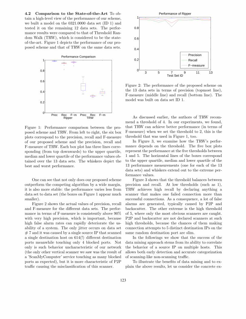
4.2 Comparison to the State-of-the-Art To ob-tain a high-level view of the performance of our scheme,we built a model on the 0321.0000 data set (ID 1) andtested it on the remaining 12 data sets. The perfor-mance results were compared to that of Threshold Ran-dom Walk (TRW), which is considered to be the state-of-the-art. Figure 1 depicts the performance of our pro-posed scheme and that of TRW on the same data sets.
Prec Rec F−m Prec Rec F−m0
0.2
0.4
0.6
0.8
1
Ripper TRW
Performance Comparison
Figure 1: Performance comparison between the pro-posed scheme and TRW. From left to right, the six boxplots correspond to the precision, recall and F-measureof our proposed scheme and the precision, recall andF-measure of TRW. Each box plot has three lines corre-sponding (from top downwards) to the upper quartile,median and lower quartile of the performance values ob-tained over the 13 data sets. The whiskers depict thebest and worst performance.
One can see that not only does our proposed schemeoutperform the competing algorithm by a wide margin,it is also more stable: the performance varies less fromdata set to data set (the boxes on Figure 1 appear muchsmaller).
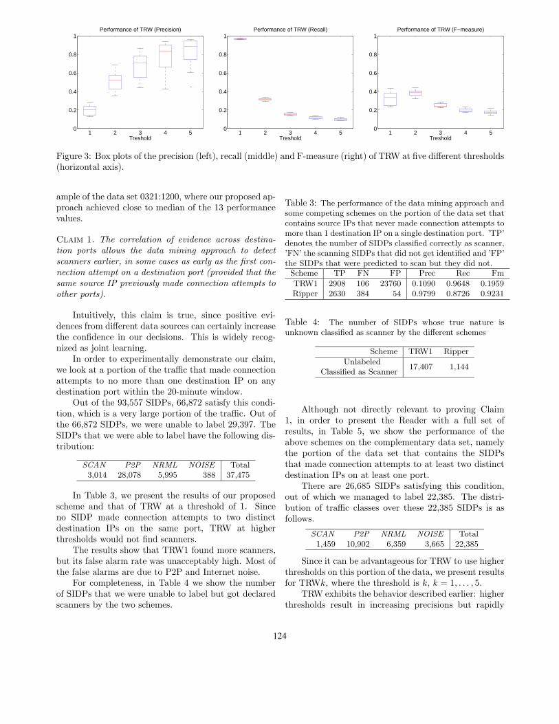
Figure 2 shows the actual values of precision, recalland F-measure for the different data sets. The perfor-mance in terms of F-measure is consistently above 90%with very high precision, which is important, becausehigh false alarm rates can rapidly deteriorate the us-ability of a system. The only jitter occurs on data set# 7 and it was caused by a single source IP that scanneda single destination host on 614(!) different destinationports meanwhile touching only 4 blocked ports. Notonly is such behavior uncharacteristic of our network(the only other vertical scanner we saw was the result ofa ’ScanMyComputer’ service touching as many blockedports as expected), but it is more characteristic of P2Ptraffic causing the misclassification of this scanner.
3 5 7 9 11 130
0.2
0.4
0.6
0.8
1
Test Set ID
Performance of Ripper
Precision
Recall
F−measure
Figure 2: The performance of the proposed scheme onthe 13 data sets in terms of precision (topmost line),F-measure (middle line) and recall (bottom line). Themodel was built on data set ID 1.
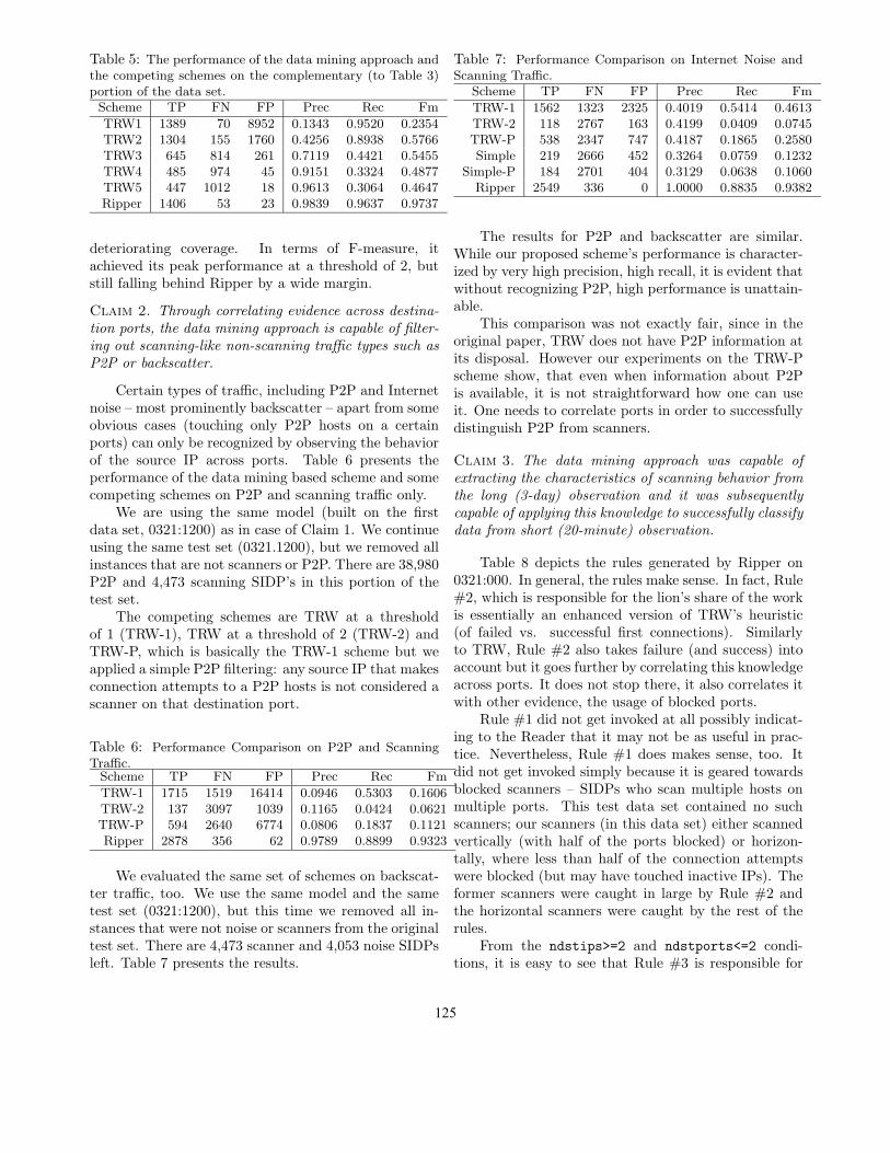
As discussed earlier, the authors of TRW recom-mend a threshold of 4. In our experiments, we found,that TRW can achieve better performance (in terms ofF-measure) when we set the threshold to 2, this is thethreshold that was used in Figure 1, too.
In Figure 3, we examine how the TRW’s perfor-mance depends on the threshold. The five box plotsrepresent the performance at the five thresholds between1 and 5. The horizontal lines of the boxes correspondto the upper quartile, median and lower quartile of the13 performance measurements (one for each of the 13data sets) and whiskers extend out to the extreme per-formance values.
Figure 3 shows that the threshold balances betweenprecision and recall. At low thresholds (such as 1),TRW achieves high recall by declaring anything ascanner that makes one failed connection more thansuccessful connections. As a consequence, a lot of falsealarms are generated, typically caused by P2P andbackscatter. The other extreme is the high thresholdof 5, where only the most obvious scanners are caught.P2P and backscatter are not declared scanners at suchhigh thresholds, because the chances of them makingconnection attempts to 5 distinct destination IPs on thesame random destination port are slim.
In the followings we show that the success of thedata mining approach stems from its ability to correlatethe behavior of a source IP on multiple hosts. Thisallows both early detection and accurate categorizationof scanning-like non-scanning traffic.
To illustrate the benefits of data mining and to ex-plain the above results, let us consider the concrete ex-
123
1 2 3 4 50
0.2
0.4
0.6
0.8
1
Treshold
Performance of TRW (Precision)
1 2 3 4 50
0.2
0.4
0.6
0.8
1
Treshold
Performance of TRW (Recall)
1 2 3 4 50
0.2
0.4
0.6
0.8
1
Treshold
Performance of TRW (F−measure)
Figure 3: Box plots of the precision (left), recall (middle) and F-measure (right) of TRW at five different thresholds(horizontal axis).
ample of the data set 0321:1200, where our proposed ap-proach achieved close to median of the 13 performancevalues.
Claim 1. The correlation of evidence across destina-tion ports allows the data mining approach to detectscanners earlier, in some cases as early as the first con-nection attempt on a destination port (provided that thesame source IP previously made connection attempts toother ports).
Intuitively, this claim is true, since positive evi-dences from different data sources can certainly increasethe confidence in our decisions. This is widely recog-nized as joint learning.
In order to experimentally demonstrate our claim,we look at a portion of the traffic that made connectionattempts to no more than one destination IP on anydestination port within the 20-minute window.
Out of the 93,557 SIDPs, 66,872 satisfy this condi-tion, which is a very large portion of the traffic. Out ofthe 66,872 SIDPs, we were unable to label 29,397. TheSIDPs that we were able to label have the following dis-tribution:
In Table 3, we present the results of our proposedscheme and that of TRW at a threshold of 1. Sinceno SIDP made connection attempts to two distinctdestination IPs on the same port, TRW at higherthresholds would not find scanners.
The results show that TRW1 found more scanners,but its false alarm rate was unacceptably high. Most ofthe false alarms are due to P2P and Internet noise.
For completeness, in Table 4 we show the numberof SIDPs that we were unable to label but got declaredscanners by the two schemes.
Table 3: The performance of the data mining approach andsome competing schemes on the portion of the data set thatcontains source IPs that never made connection attempts tomore than 1 destination IP on a single destination port. ’TP’denotes the number of SIDPs classified correctly as scanner,’FN’ the scanning SIDPs that did not get identified and ’FP’the SIDPs that were predicted to scan but they did not.Scheme TP FN FP Prec Rec Fm
Table 4: The number of SIDPs whose true nature isunknown classified as scanner by the different schemes
Scheme TRW1 Ripper
Unlabeled17,407 1,144
Classified as Scanner
Although not directly relevant to proving Claim1, in order to present the Reader with a full set ofresults, in Table 5, we show the performance of theabove schemes on the complementary data set, namelythe portion of the data set that contains the SIDPsthat made connection attempts to at least two distinctdestination IPs on at least one port.
There are 26,685 SIDPs satisfying this condition,out of which we managed to label 22,385. The distri-bution of traffic classes over these 22,385 SIDPs is asfollows.
Since it can be advantageous for TRW to use higherthresholds on this portion of the data, we present resultsfor TRWk, where the threshold is k, k = 1, . . . , 5.
TRW exhibits the behavior described earlier: higherthresholds result in increasing precisions but rapidly
124
Table 5: The performance of the data mining approach andthe competing schemes on the complementary (to Table 3)portion of the data set.Scheme TP FN FP Prec Rec Fm
deteriorating coverage. In terms of F-measure, itachieved its peak performance at a threshold of 2, butstill falling behind Ripper by a wide margin.
Claim 2. Through correlating evidence across destina-tion ports, the data mining approach is capable of filter-ing out scanning-like non-scanning traffic types such asP2P or backscatter.
Certain types of traffic, including P2P and Internetnoise – most prominently backscatter – apart from someobvious cases (touching only P2P hosts on a certainports) can only be recognized by observing the behaviorof the source IP across ports. Table 6 presents theperformance of the data mining based scheme and somecompeting schemes on P2P and scanning traffic only.
We are using the same model (built on the firstdata set, 0321:1200) as in case of Claim 1. We continueusing the same test set (0321.1200), but we removed allinstances that are not scanners or P2P. There are 38,980P2P and 4,473 scanning SIDP’s in this portion of thetest set.
The competing schemes are TRW at a thresholdof 1 (TRW-1), TRW at a threshold of 2 (TRW-2) andTRW-P, which is basically the TRW-1 scheme but weapplied a simple P2P filtering: any source IP that makesconnection attempts to a P2P hosts is not considered ascanner on that destination port.
Table 6: Performance Comparison on P2P and ScanningTraffic.
We evaluated the same set of schemes on backscat-ter traffic, too. We use the same model and the sametest set (0321:1200), but this time we removed all in-stances that were not noise or scanners from the originaltest set. There are 4,473 scanner and 4,053 noise SIDPsleft. Table 7 presents the results.
Table 7: Performance Comparison on Internet Noise andScanning Traffic.
The results for P2P and backscatter are similar.While our proposed scheme’s performance is character-ized by very high precision, high recall, it is evident thatwithout recognizing P2P, high performance is unattain-able.
This comparison was not exactly fair, since in theoriginal paper, TRW does not have P2P information atits disposal. However our experiments on the TRW-Pscheme show, that even when information about P2Pis available, it is not straightforward how one can useit. One needs to correlate ports in order to successfullydistinguish P2P from scanners.
Claim 3. The data mining approach was capable ofextracting the characteristics of scanning behavior fromthe long (3-day) observation and it was subsequentlycapable of applying this knowledge to successfully classifydata from short (20-minute) observation.
Table 8 depicts the rules generated by Ripper on0321:000. In general, the rules make sense. In fact, Rule#2, which is responsible for the lion’s share of the workis essentially an enhanced version of TRW’s heuristic(of failed vs. successful first connections). Similarlyto TRW, Rule #2 also takes failure (and success) intoaccount but it goes further by correlating this knowledgeacross ports. It does not stop there, it also correlates itwith other evidence, the usage of blocked ports.
Rule #1 did not get invoked at all possibly indicat-ing to the Reader that it may not be as useful in prac-tice. Nevertheless, Rule #1 does makes sense, too. Itdid not get invoked simply because it is geared towardsblocked scanners – SIDPs who scan multiple hosts onmultiple ports. This test data set contained no suchscanners; our scanners (in this data set) either scannedvertically (with half of the ports blocked) or horizon-tally, where less than half of the connection attemptswere blocked (but may have touched inactive IPs). Theformer scanners were caught in large by Rule #2 andthe horizontal scanners were caught by the rest of therules.
From the ndstips>=2 and ndstports<=2 condi-tions, it is easy to see that Rule #3 is responsible for
125
Table 8: The rules and their interpretations for identifyingscanners built on 0321.0000. ’Cnt’ stands for the number ofinvocations on the test set 0321.1200.ID Cnt Rule
1 0 blk >= 0.5 nosrv >= 0.6667 indstips
>= 2
More than half of the destination IPstouched were touched on blocked des-tination ports, mostly service was notoffered and the source IP touched at least2 distinct IPs on the current destinationport.
2 3764 blk >= 0.5 nosrv >= 0.7778
More then half of the IPs were touched onblocked destination ports and service isalmost never offered.
3 35 iblk >= 1 ndstips >= 2 ndstports <=
2
Connection attempts were made onno more than 2 distinct destinationports to at least 2 distinct destination IPsand the current destination port is blocked.
4 23 iblk >= 1 pp <= 0.75 ndstips <= 4
ndstports >= 5
The source IP touched at least 5 destina-tion ports out of which at least the currentport is blocked, the number of distinctdestination IPs is no more then 4 and atleast one of them is not a P2P host.q
... 6 [truncated]
identifying horizontal scanners, where the requirementof one of the (possibly two) ports being blocked providesthe evidence of scanning activity.
In our scheme, we included a whole set of featuresto enable the recognition of exceptional behaviors. Inthis rule set, Rule #4 has the ability to recognize suchsource IPs. Imagine a source IP, that engages in normaltraffic on a variety of ports but perform scans on one.As long as this source IP made connection attempts onmore than 5 destination ports, and scans on one (whichis blocked), Rule #4 will catch it. The caveat is thatP2P traffic can also exhibit this kind of behavior. P2Pfalse alarms are avoided by the pp<=.75 clause.
In the followings, let us have a look at concreteexamples describing how the rule set supports our firsttwo claims.
Early Detection. One of the most difficult tasksis to correctly recognize scanners who make connectionattempts to only one destination IP on each destinationport. The only hard evidence we can have against
such a source IP is the unexpectedly large number ofconnection attempts on blocked ports. Either Rule #1or Rule #2 will identify such scanners.
Rule # 3 is another example of correlating infor-mation. It says that if a source IP makes connectionattempts to a blocked port then making connection at-tempts on only one other port to at least two distincthosts is suspicious. Only P2P (using random ports) andbackscatter are non-scanning traffic types making con-nection attempts to blocked ports. However, the prob-ability of randomly selecting the same port for two dis-tinct destination IPs is negligible, hence such behavioris indeed very suspicious.
Detection of P2P. Rule # 4 is the only rule thatexplicitly uses the P2P feature. P2P feature is notrequired for the detection of P2P, false alarms due toP2P can be avoided by using the blocked ports. WhileP2P can possibly make connection attempts on blockedports (randomly chosen port), it is highly unlikely thatit would attempt a large portion of its communicationon blocked ports. The first three rules use 50% as the’large portion’, while Rule #4 explicitly uses the P2Pfeature.
Backscatter. There is no explicit feature pro-vided to help recognize backscatter traffic. Fortunately,(most) P2P and backscatter traffic share the commonal-ity of randomly choosing destination ports, so the mech-anism used to filter out P2P can also be used to filterout backscatter: it is highly unlikely that a large por-tion of the randomly chosen set of destination ports forbackscatter traffic will be blocked.
Table 9: Variants of Rule # 2 in Models Built on DifferentTime Intervals02 blk >= 0.5 nosrv >= 0.5476 .
03 iblk >= 1 nosrv >= 1 blk >= 0.5 .
04 blk >= 0.3333 nosrv >= 0.8889 .
08 blk >= 0.5 nosrv >= 1 .
09 blk >= 0.4 nosrv >= 0.75 .
11 blk >= 0.3333 nosrv >= 0.5 iblk >= 1 .
12 blk >= 0.3333 nosrv >= 0.5714 .
13 blk >= 0.3333 nosrv >= 0.875 .
4.2.1 Variations to Rule #2 As mentioned before,Rule #2 has the largest contribution to the high per-formance of our proposed scheme. Since this rule is sodominant, yet appears very generic, it is reasonable toassume that models built on other data sets contain sim-ilar rules. Indeed, examination of the models built onthe other 12 data sets revealed that 8 other data setshave close variants of Rule #2. Table 9 shows theserules.
The fact that the rule appears with a wide range
126
of thresholds (blk varying between .3 and .5 and nosrv
varying between .54 and 1) reassures us that the rule isindeed generic.
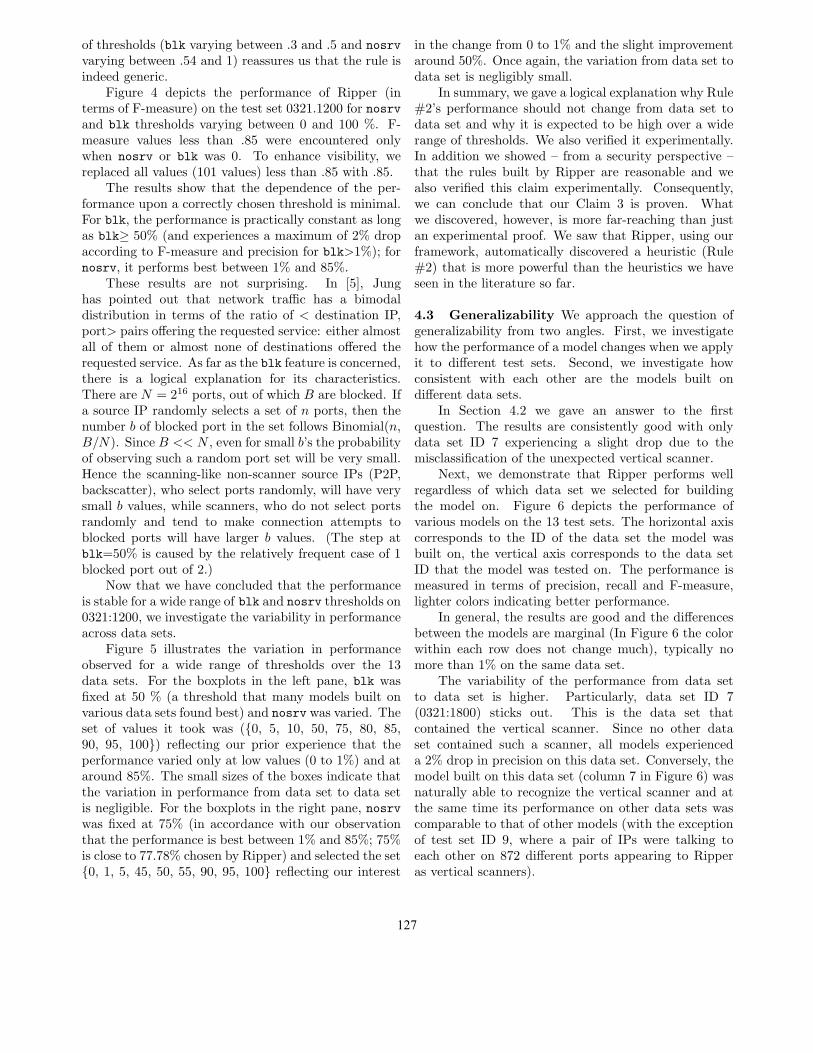
Figure 4 depicts the performance of Ripper (interms of F-measure) on the test set 0321.1200 for nosrvand blk thresholds varying between 0 and 100 %. F-measure values less than .85 were encountered onlywhen nosrv or blk was 0. To enhance visibility, wereplaced all values (101 values) less than .85 with .85.
The results show that the dependence of the per-formance upon a correctly chosen threshold is minimal.For blk, the performance is practically constant as longas blk≥ 50% (and experiences a maximum of 2% dropaccording to F-measure and precision for blk>1%); fornosrv, it performs best between 1% and 85%.
These results are not surprising. In [5], Junghas pointed out that network traffic has a bimodaldistribution in terms of the ratio of < destination IP,port> pairs offering the requested service: either almostall of them or almost none of destinations offered therequested service. As far as the blk feature is concerned,there is a logical explanation for its characteristics.There are N = 216 ports, out of which B are blocked. Ifa source IP randomly selects a set of n ports, then thenumber b of blocked port in the set follows Binomial(n,B/N). Since B << N , even for small b’s the probabilityof observing such a random port set will be very small.Hence the scanning-like non-scanner source IPs (P2P,backscatter), who select ports randomly, will have verysmall b values, while scanners, who do not select portsrandomly and tend to make connection attempts toblocked ports will have larger b values. (The step atblk=50% is caused by the relatively frequent case of 1blocked port out of 2.)
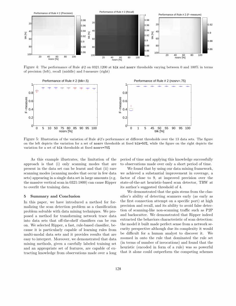
Now that we have concluded that the performanceis stable for a wide range of blk and nosrv thresholds on0321:1200, we investigate the variability in performanceacross data sets.
Figure 5 illustrates the variation in performanceobserved for a wide range of thresholds over the 13data sets. For the boxplots in the left pane, blk wasfixed at 50 % (a threshold that many models built onvarious data sets found best) and nosrv was varied. Theset of values it took was ({0, 5, 10, 50, 75, 80, 85,90, 95, 100}) reflecting our prior experience that theperformance varied only at low values (0 to 1%) and ataround 85%. The small sizes of the boxes indicate thatthe variation in performance from data set to data setis negligible. For the boxplots in the right pane, nosrvwas fixed at 75% (in accordance with our observationthat the performance is best between 1% and 85%; 75%is close to 77.78% chosen by Ripper) and selected the set{0, 1, 5, 45, 50, 55, 90, 95, 100} reflecting our interest
in the change from 0 to 1% and the slight improvementaround 50%. Once again, the variation from data set todata set is negligibly small.
In summary, we gave a logical explanation why Rule#2’s performance should not change from data set todata set and why it is expected to be high over a widerange of thresholds. We also verified it experimentally.In addition we showed – from a security perspective –that the rules built by Ripper are reasonable and wealso verified this claim experimentally. Consequently,we can conclude that our Claim 3 is proven. Whatwe discovered, however, is more far-reaching than justan experimental proof. We saw that Ripper, using ourframework, automatically discovered a heuristic (Rule#2) that is more powerful than the heuristics we haveseen in the literature so far.
4.3 Generalizability We approach the question ofgeneralizability from two angles. First, we investigatehow the performance of a model changes when we applyit to different test sets. Second, we investigate howconsistent with each other are the models built ondifferent data sets.
In Section 4.2 we gave an answer to the firstquestion. The results are consistently good with onlydata set ID 7 experiencing a slight drop due to themisclassification of the unexpected vertical scanner.
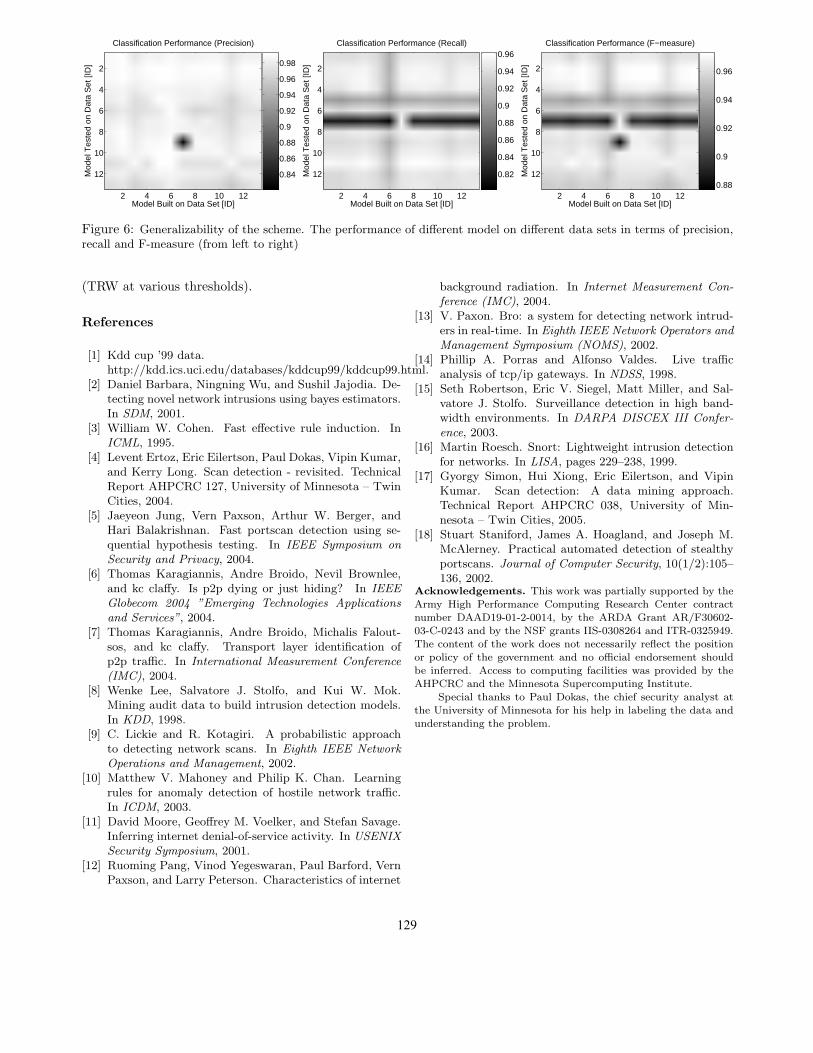
Next, we demonstrate that Ripper performs wellregardless of which data set we selected for buildingthe model on. Figure 6 depicts the performance ofvarious models on the 13 test sets. The horizontal axiscorresponds to the ID of the data set the model wasbuilt on, the vertical axis corresponds to the data setID that the model was tested on. The performance ismeasured in terms of precision, recall and F-measure,lighter colors indicating better performance.
In general, the results are good and the differencesbetween the models are marginal (In Figure 6 the colorwithin each row does not change much), typically nomore than 1% on the same data set.
The variability of the performance from data setto data set is higher. Particularly, data set ID 7(0321:1800) sticks out. This is the data set thatcontained the vertical scanner. Since no other dataset contained such a scanner, all models experienceda 2% drop in precision on this data set. Conversely, themodel built on this data set (column 7 in Figure 6) wasnaturally able to recognize the vertical scanner and atthe same time its performance on other data sets wascomparable to that of other models (with the exceptionof test set ID 9, where a pair of IPs were talking toeach other on 872 different ports appearing to Ripperas vertical scanners).
127
nosrv [%]
blk
[%]
Performance of Rule # 2 (Precision)
20 40 60 80 100
20
40
60
80
1000.86
0.88
0.9
0.92
0.94
0.96
0.98
Performance of Rule # 2 (Recall)
nosrv [%]
blk
[%]
20 40 60 80 100
20
40
60
80
100 0.84
0.86
0.88
0.9
0.92
0.94
0.96
0.98
1 Performance of Rule # 2 (F−measure)
nosrv [%]
blk
[%]
20 40 60 80 100
20
40
60
80
1000.86
0.88
0.9
0.92
Figure 4: The performance of Rule #2 on 0321.1200 at blk and nosrv thresholds varying between 0 and 100% in termsof precision (left), recall (middle) and f-measure (right)
0 5 10 50 75 80 85 90 95 1000
0.2
0.4
0.6
0.8
1
F−
mea
sure
nosrv [%]
Performance of Rule # 2 (blk=.5)
0 1 5 45 50 55 90 95 1000
0.2
0.4
0.6
0.8
1
F−
mea
sure
blk [%]
Performance of Rule # 2 (nosrv=.75)
Figure 5: Illustration of the variation of Rule #2’s performance at different thresholds over the 13 data sets. The figureon the left depicts the variation for a set of nosrv thresholds at fixed blk=50%, while the figure on the right depicts thevariation for a set of blk thresholds at fixed nosrv=75%
As this example illustrates, the limitation of theapproach is that (i) only scanning modes that arepresent in the data set can be learnt and that (ii) rarescanning modes (scanning modes that occur in few datasets) appearing in a single data set in large amounts (e.g.the massive vertical scan in 0321:1800) can cause Ripperto overfit the training data.
5 Summary and Conclusion
In this paper, we have introduced a method for for-malizing the scan detection problem as a classificationproblem solvable with data mining techniques. We pro-posed a method for transforming network trace datainto data sets that off-the-shelf classifiers can be runon. We selected Ripper, a fast, rule-based classifier, be-cause it is particularly capable of learning rules frommulti-modal data sets and it provides results that areeasy to interpret. Moreover, we demonstrated that datamining methods, given a carefully labeled training setand an appropriate set of features, are capable of ex-tracting knowledge from observations made over a long
period of time and applying this knowledge successfullyto observations made over only a short period of time.
We found that by using our data mining framework,we achieved a substantial improvement in coverage, afactor of close to 9, at improved precision over thestate-of-the-art heuristic-based scan detector, TRW atits author’s suggested threshold of 4.
We demonstrated that the gain stems from the clas-sifier’s ability of detecting scanners early (as early asthe first connection attempt on a specific port) at highprecision and recall, and its ability to avoid false detec-tion of scanning-like non-scanning traffic such as P2Pand backscatter. We demonstrated that Ripper indeedextracted the behaviors characteristic of scan detection:the model it built made perfect sense from a network se-curity perspective although due its complexity it wouldbe difficult for a human analyst to discover it. Wezoomed in onto the rule that dominated the rule set(in terms of number of invocations) and found that theheuristic (encoded in form of a rule) was so powerfulthat it alone could outperform the competing schemes
128
Model Built on Data Set [ID]
Mod
el T
este
d on
Dat
a S
et [I
D]
Classification Performance (Precision)
2 4 6 8 10 12
2
4
6
8
10
12 0.84
0.86
0.88
0.9
0.92
0.94
0.96
0.98
Model Built on Data Set [ID]
Mod
el T
este
d on
Dat
a S
et [I
D]
Classification Performance (Recall)
2 4 6 8 10 12
2
4
6
8
10
12 0.82
0.84
0.86
0.88
0.9
0.92
0.94
0.96
Model Built on Data Set [ID]
Mod
el T
este
d on
Dat
a S
et [I
D]
Classification Performance (F−measure)
2 4 6 8 10 12
2
4
6
8
10
120.88
0.9
0.92
0.94
0.96
Figure 6: Generalizability of the scheme. The performance of different model on different data sets in terms of precision,recall and F-measure (from left to right)
(TRW at various thresholds).
References
[1] Kdd cup ’99 data.http://kdd.ics.uci.edu/databases/kddcup99/kddcup99.html.
[2] Daniel Barbara, Ningning Wu, and Sushil Jajodia. De-tecting novel network intrusions using bayes estimators.In SDM, 2001.
[3] William W. Cohen. Fast effective rule induction. InICML, 1995.
[4] Levent Ertoz, Eric Eilertson, Paul Dokas, Vipin Kumar,and Kerry Long. Scan detection - revisited. TechnicalReport AHPCRC 127, University of Minnesota – TwinCities, 2004.
[5] Jaeyeon Jung, Vern Paxson, Arthur W. Berger, andHari Balakrishnan. Fast portscan detection using se-quential hypothesis testing. In IEEE Symposium onSecurity and Privacy, 2004.
[6] Thomas Karagiannis, Andre Broido, Nevil Brownlee,and kc claffy. Is p2p dying or just hiding? In IEEEGlobecom 2004 ”Emerging Technologies Applicationsand Services”, 2004.
[7] Thomas Karagiannis, Andre Broido, Michalis Falout-sos, and kc claffy. Transport layer identification ofp2p traffic. In International Measurement Conference(IMC), 2004.
[8] Wenke Lee, Salvatore J. Stolfo, and Kui W. Mok.Mining audit data to build intrusion detection models.In KDD, 1998.
[9] C. Lickie and R. Kotagiri. A probabilistic approachto detecting network scans. In Eighth IEEE NetworkOperations and Management, 2002.
[10] Matthew V. Mahoney and Philip K. Chan. Learningrules for anomaly detection of hostile network traffic.In ICDM, 2003.
[11] David Moore, Geoffrey M. Voelker, and Stefan Savage.Inferring internet denial-of-service activity. In USENIXSecurity Symposium, 2001.
[12] Ruoming Pang, Vinod Yegeswaran, Paul Barford, VernPaxson, and Larry Peterson. Characteristics of internet
background radiation. In Internet Measurement Con-ference (IMC), 2004.
[13] V. Paxon. Bro: a system for detecting network intrud-ers in real-time. In Eighth IEEE Network Operators andManagement Symposium (NOMS), 2002.
[14] Phillip A. Porras and Alfonso Valdes. Live trafficanalysis of tcp/ip gateways. In NDSS, 1998.
[15] Seth Robertson, Eric V. Siegel, Matt Miller, and Sal-vatore J. Stolfo. Surveillance detection in high band-width environments. In DARPA DISCEX III Confer-ence, 2003.
[16] Martin Roesch. Snort: Lightweight intrusion detectionfor networks. In LISA, pages 229–238, 1999.
[17] Gyorgy Simon, Hui Xiong, Eric Eilertson, and VipinKumar. Scan detection: A data mining approach.Technical Report AHPCRC 038, University of Min-nesota – Twin Cities, 2005.
[18] Stuart Staniford, James A. Hoagland, and Joseph M.McAlerney. Practical automated detection of stealthyportscans. Journal of Computer Security, 10(1/2):105–136, 2002.
Acknowledgements. This work was partially supported by the
Army High Performance Computing Research Center contract
number DAAD19-01-2-0014, by the ARDA Grant AR/F30602-
03-C-0243 and by the NSF grants IIS-0308264 and ITR-0325949.
The content of the work does not necessarily reflect the position
or policy of the government and no official endorsement should
be inferred. Access to computing facilities was provided by the
AHPCRC and the Minnesota Supercomputing Institute.
Special thanks to Paul Dokas, the chief security analyst atthe University of Minnesota for his help in labeling the data and