d Original Contribution SCATTERER NUMBER DENSITY CONSIDERATIONS IN REFERENCE PHANTOM-BASED ATTENUATION ESTIMATION NICHOLAS RUBERT and TOMY V ARGHESE Department of Medical Physics, University of Wisconsin—Madison, Madison, Wisconsin, USA (Received 19 November 2013; revised 20 January 2014; in final form 27 January 2014) Abstract—Attenuation estimation and imaging have the potential to be a valuable tool for tissue characterization, particularly for indicating the extent of thermal ablation therapy in the liver. Often the performance of attenuation estimation algorithms is characterized with numerical simulations or tissue-mimicking phantoms containing a high scatterer number density (SND). This ensures an ultrasound signal with a Rayleigh distributed envelope and a signal-to-noise ratio (SNR) approaching 1.91. However, biological tissue often fails to exhibit Rayleigh scat- tering statistics. For example, across 1647 regions of interest in five ex vivo bovine livers, we obtained an envelope SNR of 1.10 ± 0.12 when the tissue was imaged with the VFX 9L4 linear array transducer at a center frequency of 6.0 MHz on a Siemens S2000 scanner. In this article, we examine attenuation estimation in numerical phantoms, tissue-mimicking phantoms with variable SNDs and ex vivo bovine liver before and after thermal coagulation. We find that reference phantom-based attenuation estimation is robust to small deviations from Rayleigh statistics. However, in tissue with low SNDs, large deviations in envelope SNR from 1.91 lead to subsequently large increases in attenuation estimation variance. At the same time, low SND is not found to be a significant source of bias in the attenuation estimate. For example, we find that the standard deviation of attenuation slope estimates increases from 0.07 to 0.25 dB/cm-MHz as the envelope SNR decreases from 1.78 to 1.01 when estimating attenuation slope in tissue-mimicking phantoms with a large estimation kernel size (16 mm axially 3 15 mm laterally). Meanwhile, the bias in the attenuation slope estimates is found to be negligible (,0.01 dB/cm-MHz). We also compare results obtained with reference phantom-based attenuation estimates in ex vivo bovine liver and thermally coagulated bovine liver. (E-mail: [email protected]) Ó 2014 World Federation for Ultrasound in Medicine & Biology. Key Words: Attenuation, Envelope signal-to-noise ratio, Scatterer number density, Reference phantom, Thermal ablation, Liver, Multi-taper. INTRODUCTION Ultrasound imaging is a low-cost, portable imaging mo- dality, and attenuation coefficient estimation and subse- quent imaging have the potential to be a valuable tool for several clinical applications, including distinguishing between different types of breast masses (Nam et al. 2013), characterizing bone density to assess the risk of osteoporosis and bone fracture (Sasso et al. 2008; Wear 2003), diagnosing fatty infiltration in the liver (Narayana and Ophir 1983) and indicating the extent of thermal ablation therapy in the liver and other abdominal organs (Bush et al. 1993; Gertner et al. 1997; Kemmerer and Oelze 2012; Parmar and Kolios 2006; Techavipoo et al. 2004). In this article we focus on attenuation estimation in the liver and its application to assessment of the extent of thermal coagulation after thermal ablation therapy. Attenuation in thermally coagulated regions has often been found to approximately double relative to that in untreated normal liver tissue (Bush et al. 1993; Gertner et al. 1997; Kemmerer and Oelze 2012; Parmar and Kolios 2006; Techavipoo et al. 2004). In particular, Parmar and Kolios (2006) found a rela- tive increase in attenuation by a factor of 2.29 at a trans- mit center frequency of 5 MHz in ex vivo porcine liver after it was heated to 75 C for 60 min. Bush et al. (1993) estimated increases in attenuation coefficient in the frequency range 3.0 to 8.5 MHz from 32% to 192% in high-intensity focused ultrasound (HIFU) lesions approximately 10 3 30 mm in cross section in ex vivo pig livers. Gertner et al. (1997) found that the attenuation coefficient estimated at 3.5 MHz increased by a factor .1.8 in eight store-bought bovine liver samples after 30 min of heating at 70 C in a saline bath. Techavipoo Address correspondence to: Nicholas Rubert, Department of Medical Physics, 1111 Highland Avenue, WIMR, University of Wiscon- sin—Madison, Madison, WI 53705, USA. E-mail: [email protected]1 Ultrasound in Med. & Biol., Vol. -, No. -, pp. 1–17, 2014 Copyright Ó 2014 World Federation for Ultrasound in Medicine & Biology Printed in the USA. All rights reserved 0301-5629/$ - see front matter http://dx.doi.org/10.1016/j.ultrasmedbio.2014.01.022
Transcript
Ultrasound in Med. & Biol., Vol. -, No. -, pp. 1–17, 2014Copyright � 2014 World Federation for Ultrasound in Medicine & Biology
Printed in the USA. All rights reserved0301-5629/$ - see front matter
/j.ultrasmedbio.2014.01.022
http://dx.doi.org/10.1016
d Original Contribution
SCATTERER NUMBER DENSITY CONSIDERATIONS IN REFERENCEPHANTOM-BASED ATTENUATION ESTIMATION
NICHOLAS RUBERT and TOMY VARGHESE
Department of Medical Physics, University of Wisconsin—Madison, Madison, Wisconsin, USA
(Received 19 November 2013; revised 20 January 2014; in final form 27 January 2014)
AMedicasin—M
Abstract—Attenuation estimation and imaging have the potential to be a valuable tool for tissue characterization,particularly for indicating the extent of thermal ablation therapy in the liver. Often the performance of attenuationestimation algorithms is characterized with numerical simulations or tissue-mimicking phantoms containing ahigh scatterer number density (SND). This ensures an ultrasound signal with a Rayleigh distributed envelopeand a signal-to-noise ratio (SNR) approaching 1.91. However, biological tissue often fails to exhibit Rayleigh scat-tering statistics. For example, across 1647 regions of interest in five ex vivo bovine livers, we obtained an envelopeSNR of 1.10 ± 0.12 when the tissue was imaged with the VFX 9L4 linear array transducer at a center frequency of6.0 MHz on a Siemens S2000 scanner. In this article, we examine attenuation estimation in numerical phantoms,tissue-mimicking phantoms with variable SNDs and ex vivo bovine liver before and after thermal coagulation. Wefind that reference phantom-based attenuation estimation is robust to small deviations from Rayleigh statistics.However, in tissue with low SNDs, large deviations in envelope SNR from 1.91 lead to subsequently large increasesin attenuation estimation variance. At the same time, low SND is not found to be a significant source of bias in theattenuation estimate. For example, we find that the standard deviation of attenuation slope estimates increasesfrom 0.07 to 0.25 dB/cm-MHz as the envelope SNR decreases from 1.78 to 1.01 when estimating attenuation slopein tissue-mimicking phantoms with a large estimation kernel size (16 mm axially3 15 mm laterally). Meanwhile,the bias in the attenuation slope estimates is found to be negligible (,0.01 dB/cm-MHz). We also compare resultsobtained with reference phantom-based attenuation estimates in ex vivo bovine liver and thermally coagulatedbovine liver. (E-mail: [email protected]) � 2014 World Federation for Ultrasound in Medicine & Biology.
Ultrasound imaging is a low-cost, portable imaging mo-dality, and attenuation coefficient estimation and subse-quent imaging have the potential to be a valuable toolfor several clinical applications, including distinguishingbetween different types of breast masses (Nam et al.2013), characterizing bone density to assess the riskof osteoporosis and bone fracture (Sasso et al. 2008;Wear 2003), diagnosing fatty infiltration in the liver(Narayana and Ophir 1983) and indicating the extent ofthermal ablation therapy in the liver and other abdominalorgans (Bush et al. 1993; Gertner et al. 1997; Kemmererand Oelze 2012; Parmar and Kolios 2006; Techavipooet al. 2004). In this article we focus on attenuation
ddress correspondence to: Nicholas Rubert, Department ofl Physics, 1111HighlandAvenue,WIMR, University ofWiscon-adison, Madison, WI 53705, USA. E-mail: [email protected]
1
estimation in the liver and its application to assessmentof the extent of thermal coagulation after thermalablation therapy. Attenuation in thermally coagulatedregions has often been found to approximately doublerelative to that in untreated normal liver tissue (Bushet al. 1993; Gertner et al. 1997; Kemmerer and Oelze2012; Parmar and Kolios 2006; Techavipoo et al. 2004).
In particular, Parmar and Kolios (2006) found a rela-tive increase in attenuation by a factor of 2.29 at a trans-mit center frequency of 5 MHz in ex vivo porcine liverafter it was heated to 75�C for 60 min. Bush et al.(1993) estimated increases in attenuation coefficient inthe frequency range 3.0 to 8.5 MHz from 32% to 192%in high-intensity focused ultrasound (HIFU) lesionsapproximately 10 3 30 mm in cross section in ex vivopig livers. Gertner et al. (1997) found that the attenuationcoefficient estimated at 3.5 MHz increased by a factor.1.8 in eight store-bought bovine liver samples after30 min of heating at 70�C in a saline bath. Techavipoo
2 Ultrasound in Medicine and Biology Volume -, Number -, 2014
et al. (2004) examined the temperature dependence ofsound speed and attenuation in canine liver tissue andfound that the attenuation coefficient decreased slightlyas tissue was heated up to 50�C and then increased as tis-sue was heated from 50�C to 100�C. The relationship be-tween temperature and attenuation was hypothesized tobe due to tissue coagulation increasing tissue attenuationand temperature elevation decreasing tissue attenuation(Techavipoo et al. 2004). Kemmerer and Oelze (2012)found that the attenuation slope doubled from 0.2 to0.4 dB/cm-MHz over the frequency range 9–25 MHzwhen rat liver tissue was exposed to a 70�C saline bath.In these experiments, gas bubbles produced by heatingwere addressed very differently. In the saline bath exper-iments of Gertner et al. (1997), the authors stated that thetissue was degassed only before heating, whereas in theother saline bath heating experiments, tissue degassingwas not explicitly mentioned (Kemmerer and Oelze2012; Parmar and Kolios 2006; Techavipoo et al. 2004).In the HIFU experiment described in Bush et al. (1993),tissue was degassed under vacuum both before and afterHIFU exposure.
A variety of techniques have been applied to esti-mate attenuation within tissue. Several authors have pro-posed time-domain algorithms (Ghoshal and Oelze 2012;He and Greenleaf 1986; Jang et al. 1988; Knipp et al.1997). He and Greenleaf (1986) proposed the envelopepeak method, where the ratio of the mean envelopepeak to standard deviation of envelope peaks over depthwas minimized by adjusting an attenuation-dependentgain function. Jang et al. (1988) also proposed applyingan attenuation- and depth-dependent gain to the signal en-velope to determine attenuation. In their method, the en-tropy difference between adjacent signal segments wasminimized by adjusting the attenuation estimate and anassociated depth-dependent gain function. Knipp et al.(1997) proposed a method for estimating attenuationand backscatter in an unknown sample by comparingB-mode image values with values in a look-up tabledeveloped for individual transducers from phantomswith known attenuation and backscatter coefficients.This method had the disadvantage of requiring determi-nation of an effective frequency to assign to the recordedB-mode image to account for frequency dependence ofbeamforming, backscatter and attenuation. Ghoshal andOelze (2012) recently proposed a time-domain algorithmwhere they explicitly modeled the diffraction pattern for asingle-element circular transducer and iteratively solvedfor the attenuation coefficient in an unknown sample.
Frequency-domain techniques are currently themore popular method for determining the attenuation co-efficient in tissue. Frequency-domain techniques arefrequently described in analogy to two techniquesexplored by Kuc (1984): the spectral shift method and
the spectral difference method. In Kuc’s (1984) approach,the ultrasound signal before propagating through tissue ismodeled by a pulse power spectrum, Pi(f). The effect oftraveling through a thickness of tissue, D, is to multiplythe pulse power spectrum by an attenuation transfer func-tion, jH(f)j2 5 exp (–4pbfD), where the attenuation coef-ficient is assumed to have a linear frequency dependence.After making a round trip through tissue, the pulse powerspectrum is then given by Pf(f) 5 Pi(f) exp (–4pbfD).
In the spectral shift method, Pi(f) is modeled by aGaussian function, and the effect of attenuation is to shiftthe center frequency of the Gaussian spectrum by anamount proportional to b. The attenuation coefficientcan then be obtained by tracking the center frequencyof the ultrasound pulse with depth. In the spectral differ-ence method, the logarithm of the ratio of the power spec-tral magnitude is examined. To estimate b, log spectralratios are directly computed and no parametric modelfor the pulse spectrum is necessary. The spectral shiftand spectral difference techniques as described by Kuc(1984) failed to account for the effect of transducerbeam diffraction and focusing effects. Insana et al.(1983) developed correction factors to the spectral differ-ence method to account for beam diffraction when mak-ing attenuation measurements in tissue-mimicking (TM)phantoms with known attenuation coefficients. Madsenet al. (1984) derived a frequency-domain model for theecho signal voltage for measurements of backscatter co-efficients. This model was applied to estimation of back-scatter using single-element transducers, where beamdiffraction was accounted for using the signal spectrumfrom reflections off a reference planar reflector. Thesignal model of Madsen et al. (1984) was later extendedto backscatter coefficient and attenuation estimationwith clinical array transducers by Yao et al. (1990). Yaoet al. (1990) accounted for beam diffraction through divi-sion of tissue spectra by spectra acquired from a referencephantom with matched sound speed and the same ultra-sound system settings.
The reference phantom method developed by Yaoet al. (1990) may be considered a spectral differencemethod. In this method, amplitude changes in the fre-quency content of the ultrasound pulse are measuredover depth and normalized by a reference spectrumfrom a well-characterized phantom with known attenua-tion and backscatter. Attenuation is then estimated fromthe logarithm of the resulting ratio (Yao et al. 1990).Kim and Varghese (2008) later implemented a hybridmethod by incorporating the reference phantom methodfor normalizing spectra to reduce system-dependent ef-fects and then applying a Gaussian filter to the normalizedspectra. The frequency shift of the power spectrum withdepth was then detected using a cross-correlation algo-rithm (Kim and Varghese 2008). This algorithm was
Phantom-based attenuation estimation d N. RUBERT and T. VARGHESE 3
found to be less sensitive to artifacts than the referencephantom method when measuring attenuation in regionswith inhomogeneous backscatter coefficient under dif-fuse scattering conditions (Kim and Varghese 2008).Nam et al. (2011b) proposed a reference phantommethodin which the backscatter coefficient frequency depen-dence was modeled with a power law and attenuationwas assumed to have linear frequency dependence. Inthis algorithm, the backscatter and attenuation were esti-mated simultaneously by minimizing the squared errorbetween the predicted spectral ratio and the measuredspectral ratio.
The reference phantom method and its variationsmake several assumptions about the tissue being imaged.First, this method assumes that the tissue being imagedhas a sound speed matched to the reference phantomand the assumed sound speed of the beamformer in theultrasound system. Second, it assumes that scattering oc-curs from spatially randomly distributed scatterers andtheir number density is large enough that the envelopeis Rayleigh distributed. The impact of sound speed vari-ations on attenuation estimation has been evaluated previ-ously. Omari et al. (2011) examined variations in soundspeed from 1480 to 1600 m/s at center frequencies of 4and 5 MHz, and they found that sound speed errors ledto a bias in the attenuation estimate. Meanwhile, Namet al. (2011a) found that bias in the attenuation estimatecaused by sound speed errors was worst when examiningdepths at and around the lateral focal depth.
Little attention, however, has been given to theimpact of non-Rayleigh envelope statistics on the result-ing attenuation estimate. Inmanyof the simulation studiesfor attenuation estimation, a single scatterer size and ascatterer number density (SND) greater than 10/mm3
are often used (Kim and Heo 2012; Kim andVarghese 2007, 2008; Kim et al. 2008; Labyed andBigelow 2011; Nam et al. 2011a; Omari et al. 2011,2013). This is done to yield Rayleigh scatteringstatistics. However, non-Rayleigh scattering statisticscommonly occur in ultrasound imaging. For example,cysts and fibroadenomas in the breast have been foundto possess non-Rayleigh statistics using Nakagami imag-ing (Tsui et al. 2008). TheNakagamim-parameter has alsobeen found to range from 0.55 to 0.83 in rat liver as theMetavir score of that liver increased from 0 to 4, as esti-mated from radiofrequency (RF) data recorded with a6.5-MHz-center-frequency single-element transducer(Ho et al. 2012). The Metavir scoring system was devel-oped in France for evaluating fibrosis and cirrhosis ofthe liver resulting from chronic viral hepatitis (Bedossaand Poynard 1996). Under this scoring system, a patholo-gist evaluates the liver for damage and assigns a score ofF0 through F4. A score of F0 indicates a healthy liver;F4 indicates cirrhosis; scores between F0 and F4, repre-
sent varying degrees of fibrosis. The Nakagami imagingstudy by Ho et al. (2012) indicated that healthy liver hasa low SND, and increasingly severe liver fibrosis tendsto increase the SND.
The main aim of this article was to investigate the ef-fect of SND variations on the bias and variance of refer-ence phantom attenuation estimates. To this end, SNDvariations and their impact on reference phantom attenu-ation estimates were examined with computer simula-tions and TM phantoms imaged with a clinical, lineararray transducer. These results were used to explain theresult of reference phantom-based attenuation estimatesin normal ex vivo bovine liver and thermally coagulatedex vivo bovine liver.
THEORY
Reference phantom-based attenuation estimationIn this article, we examine the reference phantom
method of Yao et al. (1990). Yao et al. (1990) derivedthe following equation relating power spectra of sampleand reference phantom to their attenuation and back-scatter coefficients:
Psðt0; f ÞPrðt0; f Þ5
Bsðf ÞBrðf Þ expððasðf Þ2arðf ÞÞ4zÞ (1)
In eqn (1), Ps(t0,f) denotes a time-varying spectrum of anRF signal from tissue, and Pr(t0,f) is a time-varying spec-trum of an RF signal from a reference phantom. By atime-varying spectrum, we mean that RF data may be re-garded as approximately stationary over a small timewin-dow centered on t0. Then for fixed t0, Ps(t0,f) is the powerspectrum estimated over frequency centered on the loca-tion t0. Bs(f) is the backscatter coefficient of a collectionof monopole scatterers in tissue, and Br(f) is the samequantity in the reference phantom. as(f) is the attenuationcoefficient at frequency f of the unknown sample, andar(f) is the attenuation coefficient at frequency f of thereference phantom. z is the imaging depth. Imaging depthand time are assumed to be related through a known andconstant sound speed, c. To compute the attenuation coef-ficient of the unknown sample at a particular frequency, itis necessary to take the logarithm of eqn (1). This yields
ln
�Psðt0; f ÞPrðt0; f Þ
�5 ln
�Bsðf ÞBrðf Þ
�1ðasðf Þ2arðf Þ4zÞ (2)
To compute the attenuation coefficient at a particularfrequency, we computed a linear fit to eqn (2) over depth.We then computed the attenuation coefficient at a singlefrequency, f, from the resulting slope and the known atten-uation coefficient of the reference phantom. In this article,we have assumed a linear frequency dependence of atten-uation with an intercept of 0. Therefore, attenuation in a
4 Ultrasound in Medicine and Biology Volume -, Number -, 2014
sample is given by as 5 bsf. To determine attenuationslope in the sample, we performed a second linear fit tothe attenuation coefficient as a function of frequency,fixing the intercept at 0. The estimated attenuation slope,best, is then given by
best 5
Pi
asðfiÞfiPi
f 2i(3)
Equation (3) is derived by minimizing the sum of squaredifferences between as(fi) and bestfi.
To compute a power spectrum, we used Thomson’s(1982) multi-taper method. In this method, an individualpower spectrum is computed by averaging multiple Four-ier spectra, each computed with a separate orthogonalwindow function. We denote the ith A-line in a 2-Dregion of interest (ROI) containing M A-lines by xi. Anestimate for the time-varying spectrum is then given bythe expression
Sk;iðt0; f Þ5���� PN21
t5 0
hkðtÞxiðt01tÞexpð2i2pftÞ����2
Pðt0; f Þ5 1
M
1
K
XM21
i5 0
XK21
k5 0
Sk;iðt0; f Þ(4)
In eqn (4), hk is the kth Slepian sequence. The power spec-trum at a particular time point t0 is given by an averageoverK tapers andMA-lines for a 2-D ROI. Improvementsto attenuation estimation with the use of the multi-tapermethod compared with other gating windows have beendiscussed by Rosado-Mendez et al. (2013). When a po-wer spectrum is computed with a multi-taper estimator,improvement in estimation variance over just a singletaper is expected when the spatial extent of the parameterestimation region is constrained (Rosado-Mendez et al.2013). All array and fast Fourier transform operationswere carried out using the Python library Numpy(Oliphant 2007).
Envelope signal-to-noise ratioIf the ultrasound signal is a result of scattering from
a large number of uniformly distributed microscopic in-homogeneities throughout a region of interest, then theultrasound RF echo signal envelope is a random signalwith values given by a Rayleigh probability density func-tion (PDF) (Wagner et al. 1983). The Rayleigh PDF forthe RF echo signal envelope is derived by modeling theultrasound signal as an analytic signal whose real andimaginary components are Gaussian distributed. TheRayleigh distribution is characterized by the ratio of themean to the standard deviation, that is, the signal-to-noise ratio (SNR). For a Rayleigh PDF, the SNR is givenby (p/4 – p)1/2, which is approximately 1.91.
ARayleigh PDF is achieved as a limiting case only asthe SND becomes large. As the number density of uniformscatterers drops below what is required for a Rayleighdistributed envelope, the envelope SNRof a random signalbegins to drop. Throughout the article we characterize thesignalswe examine according to the envelope SNRparam-eter. We estimated envelope SNR based on the equation
SNR5mE
sE
mE 51
M
XMi5 1
1
T
XTt5 1
EiðtÞ
s2E 5
1
M
XMi5 1
1
T21
XTt5 1
EiðtÞ2mE
(5)
In eqn (5), Ei(t) is the envelope value at the ith A-line in a2-D ROI containing M A-lines, at time point t of Tdiscrete points in the axial direction.
METHODS
SimulationsFrequency-domain simulations developed at the
University of Wisconsin—Madison were employed inthis study (Li and Zagzebski 1999). Two linear arraytransducers with different center frequencies (3.5 and5.5 MHz with 65% bandwidth each) were simulated.Each transducer had a maximum aperture that included128 elements. Each element was 0.2 mm wide laterallyand 10.0 mm wide elevationally. The simulated trans-ducer had a lateral and elevational focus occurring at adepth of 30.0 mm. Dynamic receive focusing was simu-lated with an f-number of 2. Two sets of simulated phan-toms with a sound speed of 1600m/s were created. At thissound speed, the wavelengths corresponding to the trans-ducer center frequencies were 0.457 and 0.291 mm,respectively. The two sets of numerical phantoms differedin their linear attenuation coefficients. One set had alinear attenuation coefficient of 0.50 dB/cm-MHz. Theother set of numerical phantoms had a linear attenuationcoefficient of 1.00 dB/cm-MHz. For each attenuationslope, the SND was varied from 0.2 to 1.0 scatterer/mm3 in increments of 0.1 and from 2 to 128 in dyadicsteps. SND’s of 12 and 96 were also simulated. The scat-tering amplitude was the same for all scatterers. Scat-tering from small particles was simulated so thefrequency dependence was given by f 2. For each SND,1000 independent A-lines were generated. Each A-linewas formed using a completely independent and randomrealization of the scattering distribution.
Tissue-mimicking phantomsTissue-mimicking phantoms with low, variable
SNDs were manufactured in our laboratory to compare
Phantom-based attenuation estimation d N. RUBERT and T. VARGHESE 5
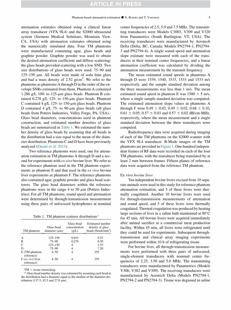
attenuation estimates obtained using a clinical lineararray transducer (VFX 9L4) and the S2000 ultrasoundsystem (Siemens Medical Solutions, Mountain View,CA, USA) with attenuation estimates obtained usingthe numerically simulated data. Four TM phantomswere manufactured containing agar, glass beads andgraphite powder. Graphite powder was used to obtainthe desired attenuation coefficient and diffuse scattering;the glass beads provided scattering with a low SND. Twosize distributions of glass beads were used: 75–90 and125–150 mm. All beads were made of soda lime glassand had a mass density of 2.52 g/cm3. We refer to thephantoms as phantoms A through D in the order of the en-velope SNRs estimated from them. Phantom A contained1.286 g/L 100- to 125-mm glass beads. Phantom B con-tained 0.278 g/L 125- to 150-mm glass beads. PhantomC contained 4 g/L 125- to 150-mm glass beads. PhantomD contained 4 g/L 75- to 90-mm glass beads (all glassbeads from Potters Industries, Valley Forge, PA, USA).-Glass bead diameters, concentrations used in phantomconstruction, and estimated number densities of glassbeads are summarized in Table 1. We estimated the num-ber density of glass beads by assuming that all beads inthe distribution had a size equal to the mean of the diam-eter distribution. Phantoms C and D have been previouslyanalyzed (Omari et al. 2013).
Two reference phantoms were used, one for attenu-ation estimation in TM phantoms A through D and a sec-ond for experiments with ex vivo bovine liver. We refer tothe reference phantom used in the TM phantom experi-ments as phantom E and that used in the ex vivo bovineliver experiments as phantom F. The reference phantomsalso contained agar, graphite powder and glass bead scat-terers. The glass bead diameters within the referencephantoms were in the range 4 to 50 mm (Potters Indus-tries). For all TM phantoms, sound speed and attenuationwere determined by through-transmission measurementusing three pairs of unfocused hydrophones at nominal
TM 5 tissue-mimicking.* Glass bead number density was estimated by assuming each bead in
the distribution had a diameter equal to the median of the diameter dis-tribution (137.5, 82.5 and 27.0 mm).
center frequencies of 2.5, 5.0 and 7.5 MHz. The transmit-ting transducers were Models C3003, V309 and V320from Panametrics (South Burlington, VT, USA). Thereceiving transducers were manufactured by AerotechDelta (Delta, BC, Canada; Models PN2794-1, PN2794-3 and PN2794-4). A single sound speed and attenuationslope estimate were measured with each of the trans-ducers at their nominal center frequencies, and a linearattenuation coefficient was calculated by dividing theattenuation measurement by the transmit frequency.
The mean estimated sound speeds in phantoms Athrough D were 1539, 1540, 1533, 1533 and 1533 m/srespectively, and the sample standard deviation amongthe three measurements was less than 1 m/s. The meanestimated sound speed in phantom E was 1580 6 5 m/s,where a single sample standard deviation was computed.The estimated attenuation slope values in phantoms Athrough F were 0.49 6 0.02, 0.49 6 0.02, 0.68 6 0.10,0.61 6 0.05, 0.57 6 0.03 and 0.57 6 0.02 dB/cm-MHz,respectively, where the mean measurement and a singlestandard deviation between the three transducers werecomputed.
Radiofrequency data were acquired during imagingof each of the TM phantoms on the S2000 scanner withthe VFX 9L4 transducer. B-Mode images of the TMphantoms are provided in Figure 1. One hundred indepen-dent frames of RF data were recorded on each of the fourTM phantoms, with the transducer being translated by atleast 2 mm between frames. Fifteen planes of referencedata were acquired from the reference TM phantom.
Ex vivo bovine liverTen independent bovine livers excised from 10 sepa-
rate animals were used in this study for reference phantomattenuation estimation, and 5 of these livers were ther-mally coagulated. Another 10 bovine livers were usedfor through-transmission measurements of attenuationand sound speed, and 5 of these livers were thermallycoagulated. Thermal coagulationwas produced by heatinglarge sections of liver in a saline bath maintained at 80�Cfor 45 min. All bovine livers were acquired immediatelyafter animal sacrifice at a commercial meat productionfacility. Within 45 min, all livers were refrigerated untilthey could be used for experiments. Subsequent through-transmission and clinical array imaging experimentswere performed within 10 h of refrigerating tissue.
For bovine liver, all through-transmission measure-ments were performed with three pairs of unfocused,single-element transducers with nominal center fre-quencies of 2.25, 3.50 and 5.0 MHz. The transmittingtransducers were manufactured by Panametrics (ModelsV306, V382 and V309). The receiving transducers weremanufactured by Aerotech Delta (Models PN2794-1,PN2794-2 and PN2794-3). Tissue was degassed in saline
Fig. 1. B-Mode images of tissue-mimicking phantoms A–D (a-d). Images were recorded with a 9L4 transducer on theSiemens S2000 with a focal depth of 3.0 cm. Image (a) exhibits the lowest envelope signal-to-noise ratio, and image
(b), the highest envelope signal-to-noise ratio.
6 Ultrasound in Medicine and Biology Volume -, Number -, 2014
solution in a low-pressure vacuum (25 mm Hg) and al-lowed to warm or cool to room temperature (22�C) beforethrough-transmission measurements. Each tissue samplewas cut in such a way as to fill a cylindrically shapedcontainer with a length of 2.50 cm and a diameter of8.00 cm. The through-transmission attenuation estimateswere made over the frequency range 1.7 to 6.3 MHz inboth normal bovine liver and thermally coagulated liver.For a single attenuation slope estimate corresponding to asingle bovine liver sample, the attenuation coefficientwas estimated in 0.1-MHz intervals over the frequencyranges 1.7–2.9, 2.8–4.2 and 4.0–6.3 MHz for the three
transducers. Overlapping measurements were averaged.Attenuation slope of ex vivo bovine liver across the fivesamples was estimated as 0.62 6 0.06 dB/cm-MHz,and that of thermally coagulated liver, 1.25 6 0.07 dB/cm-MHz. The error terms in the attenuation slope esti-mates indicate a single sample standard deviation calcu-lated using five attenuation slope estimates.
Sound speed measurements were recorded withthe same three transducers used to make attenuationmeasurements, but only at each transducer’s nominal cen-ter frequency. A sound speed of 1598 6 7 m/s wasmeasured in untreated liver tissue, and a sound speed of
Phantom-based attenuation estimation d N. RUBERT and T. VARGHESE 7
1592 6 6 m/s, in thermally coagulated tissue. The errorterms represent a single sample standard deviation forthe 15 measurements for either unheated liver or coagu-lated tissue (3 frequencies3 5 samples). In reportingthe measurements, we are assuming that dispersionwithin the samples is negligible.
All imaging was performed with the VFX 9L4 trans-ducer on the Siemens S2000 for reference phantom atten-uation estimation. Tissue was imaged in saline solution atroom temperature after degassing in a low-pressure vac-uum (25 mm Hg) and with an offset between tissue andtransducer. The offset consisted of a plastic bag contain-ing amixture of ethylene glycol and water which matchedthe tissue sound speed (1590 m/s for the thermally coag-ulated liver and 1600 m/s for the unheated liver). Thefocal depth was set between 3 and 5 cm depending onthe amount of fluid offset between tissue and transducer.Before any imaging, tissue in saline solution was de-gassed in a vacuum chamber. RF data were recordedwhile imaging a large number of independent scanningplanes in all samples: for the normal liver, 391, 316,311, 333 and 296 imaging planes (1647 total), and forthe thermally coagulated liver, 250, 286, 317, 330 and315 imaging planes (1498 total).
Reference phantom datawere recorded for both ther-mally coagulated liver tissue and untreated normal livertissue. We used a beamformer sound speed of 1590 m/sfor scanning and acquiring RF data recorded within ther-mally coagulated tissue and a sound speed of 1600 m/swhen scanning untreated normal tissue. Attenuation esti-mates in untreated normal liver tissue and thermally coag-ulated liver tissue were based on our assumption of alinear attenuation coefficient of 0.58 dB/cm-MHz forthe TM reference phantom.
When collecting reference data, we used the samebeamformer sound speed as was assumed in the tissuesamples. So, a sound speed of 1600 m/s was used whencollecting reference RF data from the TM phantom foranalyzing untreated liver tissue, and a sound speed of
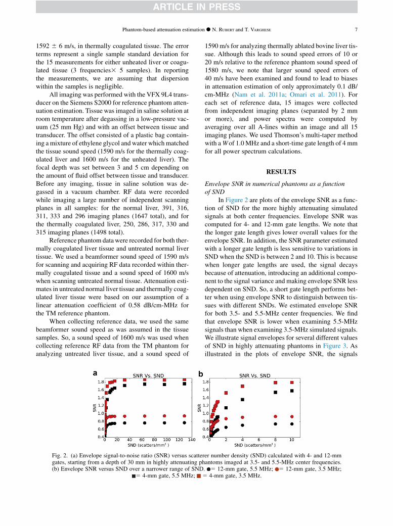
Fig. 2. (a) Envelope signal-to-noise ratio (SNR) versus scattergates, starting from a depth of 30 mm in highly attenuating ph(b) Envelope SNR versus SND over a narrower range of SND
5 4-mm gate, 5.5 MHz; 5
1590 m/s for analyzing thermally ablated bovine liver tis-sue. Although this leads to sound speed errors of 10 or20 m/s relative to the reference phantom sound speed of1580 m/s, we note that larger sound speed errors of40 m/s have been examined and found to lead to biasesin attenuation estimation of only approximately 0.1 dB/cm-MHz (Nam et al. 2011a; Omari et al. 2011). Foreach set of reference data, 15 images were collectedfrom independent imaging planes (separated by 2 mmor more), and power spectra were computed byaveraging over all A-lines within an image and all 15imaging planes. We used Thomson’s multi-taper methodwith aWof 1.0MHz and a short-time gate length of 4 mmfor all power spectrum calculations.
RESULTS
Envelope SNR in numerical phantoms as a functionof SND
In Figure 2 are plots of the envelope SNR as a func-tion of SND for the more highly attenuating simulatedsignals at both center frequencies. Envelope SNR wascomputed for 4- and 12-mm gate lengths. We note thatthe longer gate length gives lower overall values for theenvelope SNR. In addition, the SNR parameter estimatedwith a longer gate length is less sensitive to variations inSND when the SND is between 2 and 10. This is becausewhen longer gate lengths are used, the signal decaysbecause of attenuation, introducing an additional compo-nent to the signal variance and making envelope SNR lessdependent on SND. So, a short gate length performs bet-ter when using envelope SNR to distinguish between tis-sues with different SNDs. We estimated envelope SNRfor both 3.5- and 5.5-MHz center frequencies. We findthat envelope SNR is lower when examining 5.5-MHzsignals than when examining 3.5-MHz simulated signals.We illustrate signal envelopes for several different valuesof SND in highly attenuating phantoms in Figure 3. Asillustrated in the plots of envelope SNR, the signals
er number density (SND) calculated with 4- and 12-mmantoms imaged at 3.5- and 5.5-MHz center frequencies.. 5 12-mm gate, 5.5 MHz; 5 12-mm gate, 3.5 MHz;4-mm gate, 3.5 MHz.
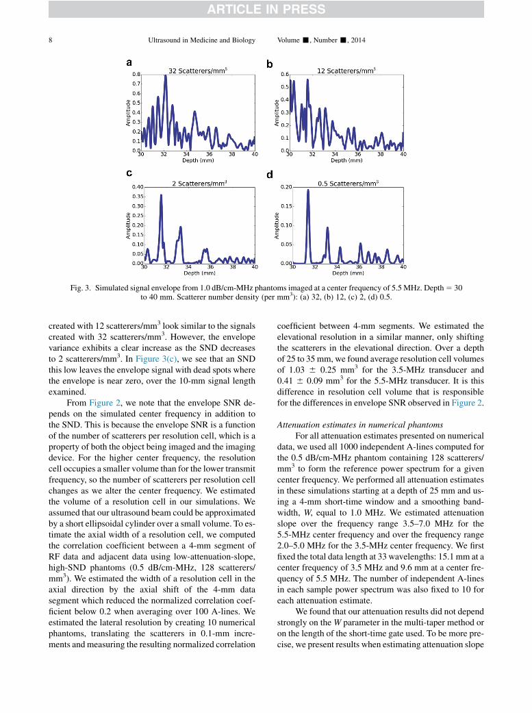
Fig. 3. Simulated signal envelope from 1.0 dB/cm-MHz phantoms imaged at a center frequency of 5.5 MHz. Depth5 30to 40 mm. Scatterer number density (per mm3): (a) 32, (b) 12, (c) 2, (d) 0.5.
8 Ultrasound in Medicine and Biology Volume -, Number -, 2014
created with 12 scatterers/mm3 look similar to the signalscreated with 32 scatterers/mm3. However, the envelopevariance exhibits a clear increase as the SND decreasesto 2 scatterers/mm3. In Figure 3(c), we see that an SNDthis low leaves the envelope signal with dead spots wherethe envelope is near zero, over the 10-mm signal lengthexamined.
From Figure 2, we note that the envelope SNR de-pends on the simulated center frequency in addition tothe SND. This is because the envelope SNR is a functionof the number of scatterers per resolution cell, which is aproperty of both the object being imaged and the imagingdevice. For the higher center frequency, the resolutioncell occupies a smaller volume than for the lower transmitfrequency, so the number of scatterers per resolution cellchanges as we alter the center frequency. We estimatedthe volume of a resolution cell in our simulations. Weassumed that our ultrasound beam could be approximatedby a short ellipsoidal cylinder over a small volume. To es-timate the axial width of a resolution cell, we computedthe correlation coefficient between a 4-mm segment ofRF data and adjacent data using low-attenuation-slope,high-SND phantoms (0.5 dB/cm-MHz, 128 scatterers/mm3). We estimated the width of a resolution cell in theaxial direction by the axial shift of the 4-mm datasegment which reduced the normalized correlation coef-ficient below 0.2 when averaging over 100 A-lines. Weestimated the lateral resolution by creating 10 numericalphantoms, translating the scatterers in 0.1-mm incre-ments and measuring the resulting normalized correlation
coefficient between 4-mm segments. We estimated theelevational resolution in a similar manner, only shiftingthe scatterers in the elevational direction. Over a depthof 25 to 35mm, we found average resolution cell volumesof 1.03 6 0.25 mm3 for the 3.5-MHz transducer and0.41 6 0.09 mm3 for the 5.5-MHz transducer. It is thisdifference in resolution cell volume that is responsiblefor the differences in envelope SNR observed in Figure 2.
Attenuation estimates in numerical phantomsFor all attenuation estimates presented on numerical
data, we used all 1000 independent A-lines computed forthe 0.5 dB/cm-MHz phantom containing 128 scatterers/mm3 to form the reference power spectrum for a givencenter frequency. We performed all attenuation estimatesin these simulations starting at a depth of 25 mm and us-ing a 4-mm short-time window and a smoothing band-width, W, equal to 1.0 MHz. We estimated attenuationslope over the frequency range 3.5–7.0 MHz for the5.5-MHz center frequency and over the frequency range2.0–5.0 MHz for the 3.5-MHz center frequency. We firstfixed the total data length at 33 wavelengths: 15.1 mm at acenter frequency of 3.5 MHz and 9.6 mm at a center fre-quency of 5.5 MHz. The number of independent A-linesin each sample power spectrum was also fixed to 10 foreach attenuation estimate.
We found that our attenuation results did not dependstrongly on theW parameter in the multi-taper method oron the length of the short-time gate used. To be more pre-cise, we present results when estimating attenuation slope
Phantom-based attenuation estimation d N. RUBERT and T. VARGHESE 9
in numerical phantoms with an SND of 4 scatterers/mm3
and an attenuation slope of 1.0 dB/cm-MHz at a centerfrequency of 5.5 MHz. In this situation, with W fixed at1.0 MHz, the attenuation slope estimates were0.99 6 0.22, 0.97 6 0.22 and 0.95 6 0.20 dB/cm-MHzas the short-time gate was varied from 3 to 4 to 5 mm,with the total parameter estimation region size kept thesame. Within the same numerical phantoms, withthe short-time gate fixed at 4 mm, we obtained attenua-tion slope estimates of 0.90 6 0.20, 0.97 6 0.22and 0.91 6 0.19 dB/cm-MHz as W was varied from0.5 to 1.0 to 1.5 MHz (multi-taper algorithm parameterNW 5 2, 4 and 7). With this in mind, we performed allfurther calculations with the short-time gate length fixedat 4 mm and W fixed at 1.0 MHz.
We plot the result of estimating attenuation inFigures 4 and 5 as the SND, and the envelope statisticswere thereby varied. In Figures 4 and 5(a), the meanvalues of the attenuation slope estimates are plotted,whereas in Figures 4 and 5(b), the variance of the attenu-ation slope estimates as a function of SND is plotted.Figures 4 and 5(c) illustrate the mean attenuation slopeestimates for a narrower range of SND, and Figures 4and 5(d) illustrate the variance in attenuation slope esti-mates for the same narrow range of SND. These figuresindicate that at an axial kernel length corresponding to33 wavelengths and a lateral kernel width correspondingto 10 independent A-lines, the attenuation estimate variedby a small amount until the envelope SNR was signifi-
Fig. 4. (a) Mean and (b) standard deviation of attenuation estimsity (SND) is varied. For all estimates, an axial kernel size of 33Same estimates as in (a, b) but over a narrower range of SND. Th
and 15.1 mm at 3.5 MHz. Std. D
cantly altered from 1.91. From the previous section, thisoccurs when the SND begins to decrease below 10scatterers/mm3.
At a center frequency of 3.5 MHz, between SNDs of10 and 128 scatterers/mm3, the mean attenuation slopeestimates were found to vary only between 0.49 and0.51 dB/cm-MHz in the less attenuating numericalphantoms and between 0.96 and 0.97 dB/cm-MHz inthe highly attenuating phantoms. The correspondingstandard deviations were found to vary between 0.08and 0.11 dB/cm-MHz in both sets of phantoms. At acenter frequency of 5.5 MHz, between SNDs of 10 and128 scatterers/mm3, the mean attenuation slope estimateswere found to vary only between 0.47 and 0.51 dB/cm-MHz in the less attenuating numerical phantoms and be-tween 0.91 and 0.98 dB/cm-MHz in the highly attenuatingphantoms. The corresponding standard deviations werefound to vary between 0.10 and 0.19 dB/cm-MHz in theless attenuating phantoms and between 0.10 and 0.15dB/cm-MHz in the more highly attenuating phantoms.
The effect that decreasing SND below 10 scatterers/mm3 had on the attenuation estimates is interesting. Thebias of the attenuation estimates exhibits no obvious trendwith decreasing SND. In the highly attenuating phan-toms, the mean attenuation slope estimate remainedwithin 16% of the true value of attenuation. In the lessattenuating phantoms, the mean attenuation estimate re-mained within 20% of the true value of the attenuationslope, except for one outlying point. The figures illustrate
ate in 1.0 dB/cm-MHz phantoms as scatterer number den-wavelengths and 10 independent A-lines were used. (c, d)irty-threewavelengths corresponds to 9.6 mm at 5.5MHzev. 5 standard deviation.
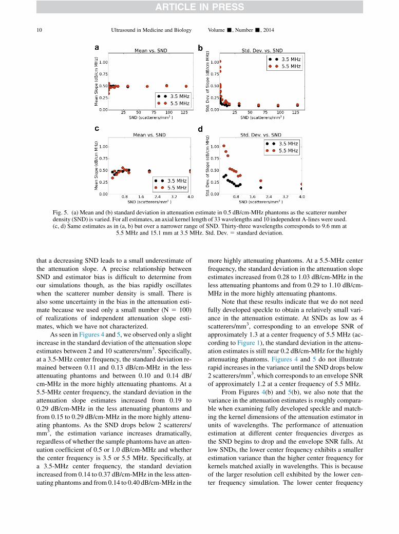
Fig. 5. (a) Mean and (b) standard deviation in attenuation estimate in 0.5 dB/cm-MHz phantoms as the scatterer numberdensity (SND) is varied. For all estimates, an axial kernel length of 33 wavelengths and 10 independent A-lines were used.(c, d) Same estimates as in (a, b) but over a narrower range of SND. Thirty-three wavelengths corresponds to 9.6 mm at
5.5 MHz and 15.1 mm at 3.5 MHz. Std. Dev. 5 standard deviation.
10 Ultrasound in Medicine and Biology Volume -, Number -, 2014
that a decreasing SND leads to a small underestimate ofthe attenuation slope. A precise relationship betweenSND and estimator bias is difficult to determine fromour simulations though, as the bias rapidly oscillateswhen the scatterer number density is small. There isalso some uncertainty in the bias in the attenuation esti-mate because we used only a small number (N 5 100)of realizations of independent attenuation slope esti-mates, which we have not characterized.
As seen in Figures 4 and 5, we observed only a slightincrease in the standard deviation of the attenuation slopeestimates between 2 and 10 scatterers/mm3. Specifically,at a 3.5-MHz center frequency, the standard deviation re-mained between 0.11 and 0.13 dB/cm-MHz in the lessattenuating phantoms and between 0.10 and 0.14 dB/cm-MHz in the more highly attenuating phantoms. At a5.5-MHz center frequency, the standard deviation in theattenuation slope estimates increased from 0.19 to0.29 dB/cm-MHz in the less attenuating phantoms andfrom 0.15 to 0.29 dB/cm-MHz in the more highly attenu-ating phantoms. As the SND drops below 2 scatterers/mm3, the estimation variance increases dramatically,regardless of whether the sample phantoms have an atten-uation coefficient of 0.5 or 1.0 dB/cm-MHz and whetherthe center frequency is 3.5 or 5.5 MHz. Specifically, ata 3.5-MHz center frequency, the standard deviationincreased from 0.14 to 0.37 dB/cm-MHz in the less atten-uating phantoms and from 0.14 to 0.40 dB/cm-MHz in the
more highly attenuating phantoms. At a 5.5-MHz centerfrequency, the standard deviation in the attenuation slopeestimates increased from 0.28 to 1.03 dB/cm-MHz in theless attenuating phantoms and from 0.29 to 1.10 dB/cm-MHz in the more highly attenuating phantoms.
Note that these results indicate that we do not needfully developed speckle to obtain a relatively small vari-ance in the attenuation estimate. At SNDs as low as 4scatterers/mm3, corresponding to an envelope SNR ofapproximately 1.3 at a center frequency of 5.5 MHz (ac-cording to Figure 1), the standard deviation in the attenu-ation estimates is still near 0.2 dB/cm-MHz for the highlyattenuating phantoms. Figures 4 and 5 do not illustraterapid increases in the variance until the SND drops below2 scatterers/mm3, which corresponds to an envelope SNRof approximately 1.2 at a center frequency of 5.5 MHz.
From Figures 4(b) and 5(b), we also note that thevariance in the attenuation estimates is roughly compara-ble when examining fully developed speckle and match-ing the kernel dimensions of the attenuation estimator inunits of wavelengths. The performance of attenuationestimation at different center frequencies diverges asthe SND begins to drop and the envelope SNR falls. Atlow SNDs, the lower center frequency exhibits a smallerestimation variance than the higher center frequency forkernels matched axially in wavelengths. This is becauseof the larger resolution cell exhibited by the lower cen-ter frequency simulation. The lower center frequency
Phantom-based attenuation estimation d N. RUBERT and T. VARGHESE 11
simulation contains more scatterers per resolution celland has a higher envelope SNR for the same SND.
We note that the results in Figures 4 and 5 are depen-dent on the spatial resolution of the attenuation estimatethat we are attempting to achieve. We next examine twolow-SND cases and vary the axial kernel length used toobtain the estimate. Figures 6 and 7(a, b) illustrate themean and variance in the attenuation estimates as a func-tion of axial kernel length when the SND is fixed at 0.6and 0.3 scatterer/mm3. From this figure, we see that alow estimation variance may still be achieved even ifthe SND becomes extremely low, as long as resolutionis sacrificed. We note that the maximum variation in themean attenuation estimates among both low and highlyattenuating phantoms as the axial kernel length is doubledover both center frequencies is 0.09 dB/cm-MHz. How-ever, the variance in the estimate exhibits a large de-crease, especially when the SND is 0.3 scatterer/mm3
and the transducer center frequency is high. At 5.5-MHz center frequency and 0.3 scatterer/mm3, the stan-dard deviation in the attenuation estimates decreasesfrom 0.72 to 0.27 dB/cm-MHz in the highly attenuatingnumerical phantoms as the axial kernel length is doubled.From all these simulations, we conclude that the SND isan important parameter in attenuation estimation. WhenSND becomes extremely low, either estimator variancewill significantly increase or estimator resolution mustsignificantly decrease to counter the increased variance.
Fig. 6. (a) Mean and (b) standard deviation of attenuation estlength is varied and the number of A-lines in the estimate is fiand (d) variance of attenuation estimates in 1.0 dB/cm-MHz pha
of A-lines in the estimate is fixed at 10 when the SND is
Reference phantom attenuation estimates in TMphantoms
For the purposes of the analysis in this section we as-sume sound speeds of 1540 m/s in TM phantoms Athrough E. We use this sound speed simply because it iscommonly assumed by most commercial ultrasound sys-tems, and the discrepancy with the measured sound speedis quite small.We reiterate that a much larger sound speedof 40 m/s is expected to cause an attenuation estimationbias of only 0.1 dB/cm-MHz (Nam et al. 2011a; Omariet al. 2011). Estimates of envelope SNR within eachphantom are listed in Table 2. Envelope SNR estimateswere made with 4-mm kernels axially and were averagedover a 16 3 15-mm ROI in the center of each imagingplane. We note that our own results indicate an increasein envelope SNR with increasing glass bead number den-sity. However, the effective SND is not necessarily thesame as the estimated number density of glass beads,even if our beads have a symmetric Gaussian distribution.This is because scattering is frequency dependent andsome sizes will contribute to the signal more than othersfor a transducer with any given center frequency andbandwidth (Chen et al. 1994).
We performed attenuation estimation as described inthe previous section. A linear attenuation coefficient of0.56 dB/cm-MHz was measured in the reference phan-tom. Power spectrum estimates were obtained usingThomson’s multi-taper estimator with a short-time gate
imates in 1.0 dB/cm-MHz phantoms as the axial kernelxed at 10 when the SND is 0.6 scatterer/mm3. (c) Meanntoms as the axial kernel length is varied and the number0.1 scatterer/mm3. Std. Dev. 5 standard deviation.
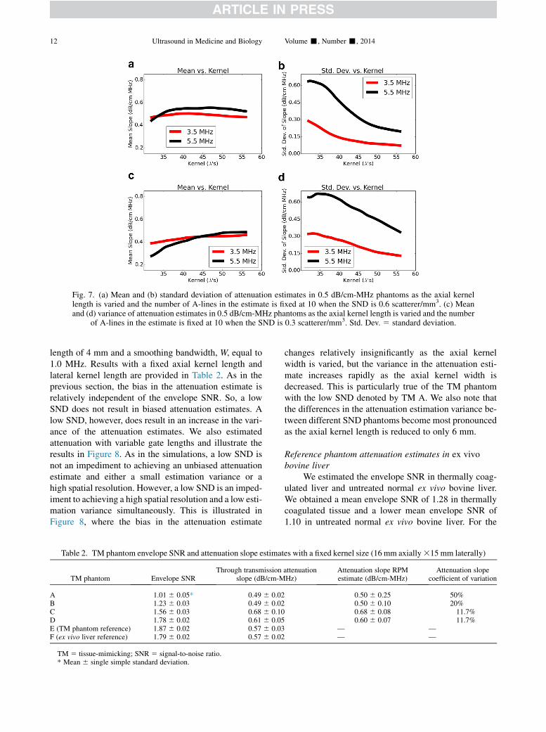
Fig. 7. (a) Mean and (b) standard deviation of attenuation estimates in 0.5 dB/cm-MHz phantoms as the axial kernellength is varied and the number of A-lines in the estimate is fixed at 10 when the SND is 0.6 scatterer/mm3. (c) Meanand (d) variance of attenuation estimates in 0.5 dB/cm-MHz phantoms as the axial kernel length is varied and the number
of A-lines in the estimate is fixed at 10 when the SND is 0.3 scatterer/mm3. Std. Dev. 5 standard deviation.
12 Ultrasound in Medicine and Biology Volume -, Number -, 2014
length of 4 mm and a smoothing bandwidth, W, equal to1.0 MHz. Results with a fixed axial kernel length andlateral kernel length are provided in Table 2. As in theprevious section, the bias in the attenuation estimate isrelatively independent of the envelope SNR. So, a lowSND does not result in biased attenuation estimates. Alow SND, however, does result in an increase in the vari-ance of the attenuation estimates. We also estimatedattenuation with variable gate lengths and illustrate theresults in Figure 8. As in the simulations, a low SND isnot an impediment to achieving an unbiased attenuationestimate and either a small estimation variance or ahigh spatial resolution. However, a low SND is an imped-iment to achieving a high spatial resolution and a low esti-mation variance simultaneously. This is illustrated inFigure 8, where the bias in the attenuation estimate
Table 2. TM phantom envelope SNR and attenuation slope estimat
TM 5 tissue-mimicking; SNR 5 signal-to-noise ratio.* Mean 6 single simple standard deviation.
changes relatively insignificantly as the axial kernelwidth is varied, but the variance in the attenuation esti-mate increases rapidly as the axial kernel width isdecreased. This is particularly true of the TM phantomwith the low SND denoted by TM A. We also note thatthe differences in the attenuation estimation variance be-tween different SND phantoms become most pronouncedas the axial kernel length is reduced to only 6 mm.
Reference phantom attenuation estimates in ex vivobovine liver
We estimated the envelope SNR in thermally coag-ulated liver and untreated normal ex vivo bovine liver.We obtained a mean envelope SNR of 1.28 in thermallycoagulated tissue and a lower mean envelope SNR of1.10 in untreated normal ex vivo bovine liver. For the
es with a fixed kernel size (16 mm axially315 mm laterally)
Fig. 8. Attenuation slope estimates as a function of axial kernel length with the lateral kernel width fixed at 15.0 mm. (a)Mean estimate versus axial kernel length in tissue-mimicking (TM) phantoms. (b) Standard deviation of estimates as afunction of axial kernel length. Images were recorded with a 9L4 transducer on the Siemens S2000 with a focal depth
of 3.0 cm. 5 TM A, 5 TM B, 5 TM C, 5 TM D, Std. Dev. 5 standard deviation.
Phantom-based attenuation estimation d N. RUBERT and T. VARGHESE 13
envelope SNR estimates, one 16 3 15-mm ROI fromeach image was subdivided into non-overlapping 4-mmaxial sub-regions, and the envelope SNR within a singleROI was the average of envelope SNR over the sub-regions. The simulations in combination with Tables 3and 4 inform us that ex vivo liver tissue exhibits envelopestatistics on the threshold of the low SND regimedescribed in the simulated data. With this in mind, we firstexamine the estimation variance estimated over all liversamples as a function of gate length in both coagulatedand untreated liver in Figure 9. A single attenuation esti-mate was made in each imaging plane around the focusdepth of the transducer. Each attenuation estimation re-gion was laterally centered in the image.
As in the simulations and TM phantom results, theestimation variance is a strong function of the parameterestimation region size, and the estimation bias variedmuch less than the estimation variance. This can beseen by comparing (a) and (b) in Figure 9. Over the rangeof parameter estimation region sizes examined, we foundthat the mean attenuation estimate in the liver variedonly between 0.43 and 0.51 dB/cm-MHz, whereas the
Table 3. Envelope SNR and attenuation slope estimatesin individual untreated normal bovine livers and alluntreated normal bovine liver for a large kernel size
TM 5 tissue-mimicking; SNR 5 signal-to-noise ratio.* Mean 6 single simple standard deviation.
standard deviation in the attenuation estimate decreasedfrom 1.80 to 0.52 dB/cm-MHz. Meanwhile, the meanattenuation estimate in the thermally coagulated livervaried only between 0.96 and 1.12 dB/cm-MHz, whereasthe standard deviation in the attenuation estimatedecreased from 1.65 to 0.50 dB/cm-MHz. The largedecrease in estimation variance with increasing axialkernel length suggests that a very small variance in theattenuation estimate may be achievable in the liver iflarger sections of tissue are imaged, degrading the spatialresolution.
Results of attenuation estimation with a large, fixedkernel within each of the individual livers are provided inFigure 10 and Tables 3 and 4. Even at a large axial kernellength of 16 mm, the standard deviation in the estimatesfor attenuation in thermally coagulated tissue wasapproximately 50% of the mean value. This value waseven higher in the untreated normal tissue, for whichthe coefficient of variation was approximately 100% ata large gate length. The lower performance in untreatednormal liver could be expected because the envelopeSNR was lowest before thermal coagulation.
Table 4. Envelope SNR and attenuation slope estimatesin individual heated bovine livers and all heated bovinelivers for a large kernel size (16 mm axially 315 mm
SNR 5 signal-to-noise ratio.* Mean 6 single simple standard deviation.
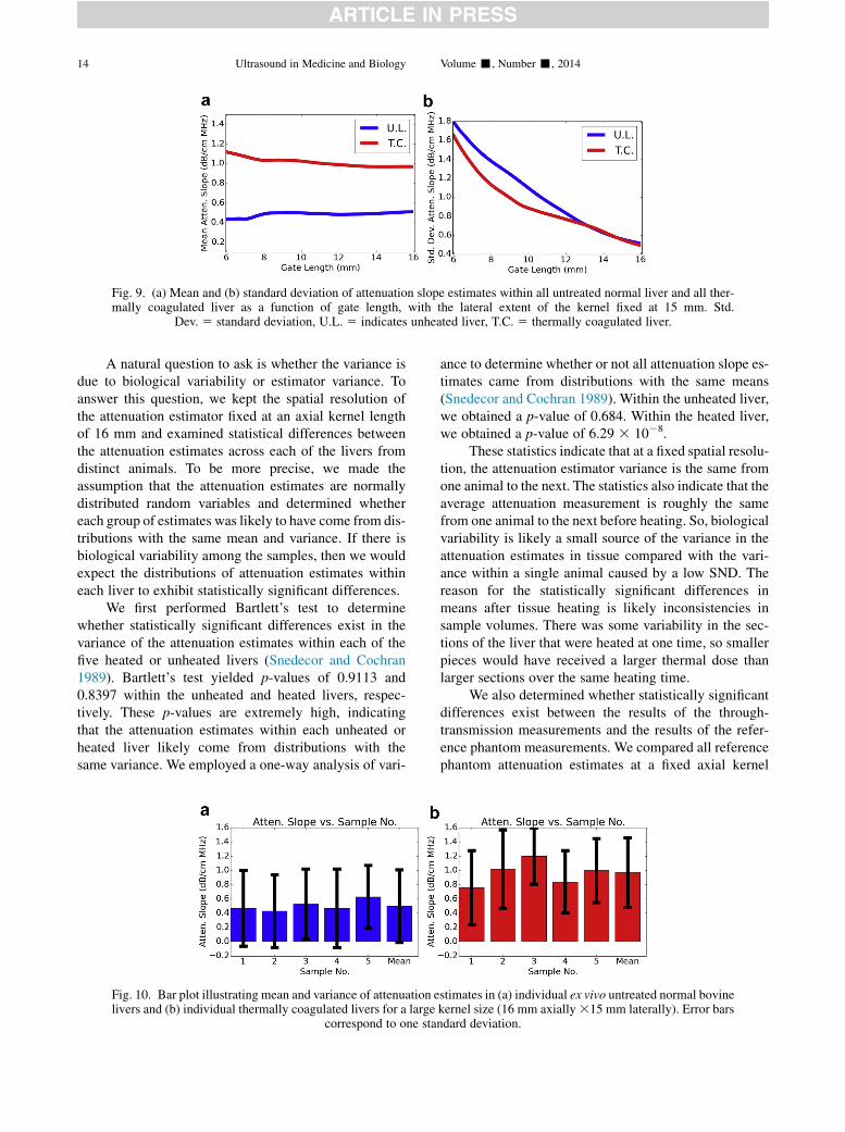
Fig. 9. (a) Mean and (b) standard deviation of attenuation slope estimates within all untreated normal liver and all ther-mally coagulated liver as a function of gate length, with the lateral extent of the kernel fixed at 15 mm. Std.
14 Ultrasound in Medicine and Biology Volume -, Number -, 2014
A natural question to ask is whether the variance isdue to biological variability or estimator variance. Toanswer this question, we kept the spatial resolution ofthe attenuation estimator fixed at an axial kernel lengthof 16 mm and examined statistical differences betweenthe attenuation estimates across each of the livers fromdistinct animals. To be more precise, we made theassumption that the attenuation estimates are normallydistributed random variables and determined whethereach group of estimates was likely to have come from dis-tributions with the same mean and variance. If there isbiological variability among the samples, then we wouldexpect the distributions of attenuation estimates withineach liver to exhibit statistically significant differences.
We first performed Bartlett’s test to determinewhether statistically significant differences exist in thevariance of the attenuation estimates within each of thefive heated or unheated livers (Snedecor and Cochran1989). Bartlett’s test yielded p-values of 0.9113 and0.8397 within the unheated and heated livers, respec-tively. These p-values are extremely high, indicatingthat the attenuation estimates within each unheated orheated liver likely come from distributions with thesame variance. We employed a one-way analysis of vari-
Fig. 10. Bar plot illustrating mean and variance of attenuation elivers and (b) individual thermally coagulated livers for a large
correspond to one stan
ance to determine whether or not all attenuation slope es-timates came from distributions with the same means(Snedecor and Cochran 1989). Within the unheated liver,we obtained a p-value of 0.684. Within the heated liver,we obtained a p-value of 6.29 3 1028.
These statistics indicate that at a fixed spatial resolu-tion, the attenuation estimator variance is the same fromone animal to the next. The statistics also indicate that theaverage attenuation measurement is roughly the samefrom one animal to the next before heating. So, biologicalvariability is likely a small source of the variance in theattenuation estimates in tissue compared with the vari-ance within a single animal caused by a low SND. Thereason for the statistically significant differences inmeans after tissue heating is likely inconsistencies insample volumes. There was some variability in the sec-tions of the liver that were heated at one time, so smallerpieces would have received a larger thermal dose thanlarger sections over the same heating time.
We also determined whether statistically significantdifferences exist between the results of the through-transmission measurements and the results of the refer-ence phantom measurements. We compared all referencephantom attenuation estimates at a fixed axial kernel
stimates in (a) individual ex vivo untreated normal bovinekernel size (16 mm axially315 mm laterally). Error barsdard deviation.
Fig. 11. Histogram illustrating approximately symmetric distri-butions of attenuation estimates in all untreated normal liversand all thermally coagulated livers. The kernel size was also16 mm axially 3 15 mm laterally. U.L. 5 indicates unheated
liver, T.C. 5 thermally coagulated liver.
Phantom-based attenuation estimation d N. RUBERT and T. VARGHESE 15
length of 16 mm with all five through-transmissionmeasurements for heated and unheated liver. Welch’stwo-sample t-test (Snedecor and Cochran 1989) indicatedstatistically significant differences between through-transmission measurements and reference phantom mea-surements with p-values of 0.0002 in both heated andunheated liver.
On the basis of the results presented in this section,we remark that the error bars are large enough so as toobtain negative values for the attenuation coefficient.Although a negative attenuation value is not physicallypossible, there is no constraint in the reference phantomalgorithm that precludes it from obtaining such a result.Figure 11 is a histogram of all the attenuation estimates.Observe that the estimates take on an approximatelyGaussian, symmetric appearance. Negative attenuationvalues are then just a logical consequence of the estima-tion variance being extremely high.
DISCUSSION
As reported by previous authors, we found that thepotential attenuation contrast between treated (coagu-lated) liver tissue and untreated liver tissue is high(Bush et al. 1993; Damianou et al. 1997; Gertner et al.1997; Kemmerer and Oelze 2012; Parmar and Kolios2006; Techavipoo et al. 2004; Worthington and Sherar2001). Using a linear model for the attenuationcoefficient, in ex vivo bovine liver, we obtained averageattenuation coefficients of approximately 0.5 dB/cm-MHz before thermal coagulation and 1.0 dB/cm-MHzafter thermal coagulation. These results are slightlylower than the attenuation coefficients we reported forthrough-transmission measurements (0.62 and 1.25 dB/
cm-MHz).We believe the through-transmission measure-ments are overestimates. Overestimation occurred be-cause it was difficult to slice tissue samples to perfectlyflat cylindrical shapes the same size as their container.This led to a small gap between the saran cover of thesample holder and the tissue sample, additional reflectionlosses and overestimation of the attenuation coefficient.
In this article, we have described the difficultyinvolved in obtaining attenuation images in the liverwith low variance and high spatial resolution. This ex-plains the large number of articles in the literature ad-dressing the attenuation contrast between thermallycoagulated liver and untreated liver (Bush et al. 1993;Gertner et al. 1997; Kemmerer and Oelze 2012; Parmarand Kolios 2006; Techavipoo et al. 2004), the largenumber of articles providing reference phantom-basedattenuation imaging results (Kim and Heo 2012; Kimand Varghese 2007, 2008; Kim et al. 2008; Labyed andBigelow 2011; Nam et al. 2011a; Omari et al. 2011,2013), but the limited results demonstrating attenuationimages of thermal coagulations.
Imaging in an ex vivo setting is one of the first steps invalidating algorithms to be applied to the clinical abdom-inal ultrasound setting. In an ex vivo setting, the confound-ing effects on the imaging of fat and muscle layersintervening between the liver and the transducer may beavoided. However, we found that the scattering weobserved in the liver deviates significantly from the scat-tering model that has been frequently assumed whendeveloping reference phantom and other algorithms forattenuation estimation. We hypothesize that the sparsescattering responsible for the low envelope SNR arisesfrom the portal triads, while hepatocytes provide the un-derlying low-level scattering. This sort of scatteringmodelis frequently employedwhen analyzing periodic scatteringand mean scattering spacing in the liver (Fellingham andSommer 1984; Machado et al. 2006; Rubert andVarghese 2013, 2014; Varghese and Donohue 1993).
The estimation variance for attenuation slope esti-mation is highly dependent on the envelope SNR.Although our own results indicated a low envelopeSNR in an ex vivo setting, we note that the effect ofexcising liver from an animal on the envelope statisticsof a liver has not been investigated. We noted that smalldifferences in envelope SNR had a large effect on theattenuation estimation variance once the SNR began tosignificantly deviate from 1.91. Ex vivo porcine (Bushet al. 1993; Zhou et al. 2013), bovine (Bevan andSherar 2001a, 2001b; Dewall et al. 2010; Gertner et al.1997; Luchies et al. 2012; Parker 1983; Pereira andMaciel 2001), rat (Kemmerer and Oelze 2012) and hu-man (Machado et al. 2006) livers have all been used forthe development of ultrasonic tissue characterizationalgorithms based on features extracted from RF data.
16 Ultrasound in Medicine and Biology Volume -, Number -, 2014
However, we are not aware of any studies comparingestimates of envelope statistics in excised liver with esti-mates of envelope statistics in an in vivo setting. In com-parison of ex vivo and in vivo measurements of envelopeSNR, there are two effects to consider: (i) the changingsize of a resolution cell dependent on the propagationpath and (ii) the immediate drop in blood pressure andloss of perfusion that occur when a liver is excised.
To match the resolution cell size, comparisonscould be made between RF data recorded with an animalunder open surgery conditions and an excised liver usingthe same transducer and imaging settings at the samedepth. An open surgery model would avoid the broad-ening of a resolution cell that occurs from phase aberra-tion within layers of skin, fat and abdominal muscle thatare encountered when imaging the liver in vivo. Withidentical resolution cell volumes, the envelope SNRwould reflect only differences in the state of the tissue.The pathologic state of the tissue and the species underconsideration also are likely to have an effect on enve-lope statistics. Envelope SNR or some other metric ofscatterer number density must be well characterized intissue to develop bounds on reference phantom-basedattenuation estimation variance.
CONCLUSIONS
The results in this article indicate that for tissueexhibiting a Rayleigh distributed envelope distribution,a low-variance, high-resolution attenuation image maybe generated using the reference phantom methoddeveloped by Yao et al. (1990) in conjunction with amulti-taper spectral estimate. Attenuation imagingholds great promise for delineating the extent of ther-mally coagulated tissue during thermal therapy in theliver. Using both through-transmission measurementsand reference phantom attenuation estimates, we foundthat the attenuation slope approximately doubles afterdelivery of a large thermal dose to liver tissue. Howev-er, across a large number of ROIs (N 5 1647) in 5ex vivo bovine livers, we calculated an envelope SNRof 1.1. We found that the large variance in the envelopemagnitude caused by scattering results in a large vari-ance in reference phantom attenuation estimates andis currently an obstacle to the use of referencephantom-based attenuation imaging for delineating theextent of thermally coagulated regions.
Acknowledgments—This workwas supported byGrants R01CA112192-S103, R01CA112192-06 and T32 CA09206-32 from the National Can-cer Institute, National Institutes of Health. The authors thankGary Frankfor construction of the tissue-mimicking phantoms. The authors alsothank Black Earth Meats, Black Earth, Wisconsin, for providing thebovine liver samples.
REFERENCES
Bedossa P, Poynard T. An algorithm for the grading of activity in chronichepatitis C. Hepatology 1996;24:289–293.
Bevan PD, Sherar MD. B-Scan ultrasound imaging of thermal coagula-tion in bovine liver: Frequency shift attenuation mapping. Ultra-sound Med Biol 2001a;27:809–817.
Bevan PD, Sherar MD. B-scan ultrasound imaging of thermal coagula-tion in bovine liver: Log envelope slope attenuation mapping. Ultra-sound Med Biol 2001b;27:379–387.
Bush NL, Rivens I, Ter Haar GR, Bamber JC. Acoustic properties oflesions generated with an ultrasound therapy system. UltrasoundMed Biol 1993;19:789–801.
Chen JF, Madsen EL, Zagzebski JA. A method for determination offrequency-dependent effective scatterer number density. J AcoustSoc Am 1994;95:77–85.
Damianou CA, Sanghvi NT, Fry FJ, Maass-Moreno R. Dependence ofultrasonic attenuation and absorption in dog soft tissues on temper-ature and thermal dose. J Acoust Soc Am 1997;102:628–634.
Dewall R, Varghese T, Madsen E. Shear wave velocity imaging usingtransient electrode perturbation: Phantom and ex vivo validation.IEEE Trans Med Imaging 2010;30:666–678.
Fellingham LL, Sommer FG. Ultrasonic characterization of tissue struc-ture in the in vivo human liver and spleen. IEEE Trans UltrasonFerroelectr Freq Control 1984;31:418–428.
Gertner MR, Wilson BC, Sherar MD. Ultrasound properties of livertissue during heating. Ultrasound Med Biol 1997;23:1395–1403.
Ghoshal G, Oelze ML. Time domain attenuation estimation methodfrom ultrasonic backscattered signals. J Acoust Soc Am 2012;132:533–543.
He P, Greenleaf JF. Attenuation estimation on phantoms—A stabilitytest. Ultrason Imaging 1986;8:1–10.
Ho MC, Lin JJ, Shu YC, Chen CN, Chang KJ, Chang CC, Tsui PH.Using ultrasound Nakagami imaging to assess liver fibrosis in rats.Ultrasonics 2012;52:215–222.
Insana M, Zagzebski J, Madsen E. Improvements in the spectral differ-ence method for measuring ultrasonic attenuation. Ultrason Imaging1983;5:331–345.
Jang HS, Song TK, Park SB. Ultrasound attenuation estimation in softtissue using the entropy difference of pulsed echoes between twoadjacent envelope segments. Ultrason Imaging 1988;10:248–264.
Kemmerer JP, Oelze ML. Ultrasonic assessment of thermal therapy inrat liver. Ultrasound Med Biol 2012;38:2130–2137.
Kim H, Heo SW. Time-domain calculation of spectral centroid frombackscattered ultrasound signals. IEEE Trans Ultrason FerroelectrFreq Control 2012;59:1193–1200.
Kim H, Varghese T. Attenuation estimation using spectral cross-correla-tion. IEEETransUltrasonFerroelectr FreqControl 2007;54:510–519.
Kim H, Varghese T. Hybrid spectral domain method for attenuationslope estimation. Ultrasound Med Biol 2008;34:1808–1819.
Kim H, Zagzebski JA, Varghese T. Estimation of ultrasound attenuationfrom broadband echo-signals using bandpass filtering. IEEE TransUltrason Ferroelectr Freq Control 2008;55:1153–1159.
Knipp BS, Zagzebski JA, Wilson TA, Dong F, Madsen EL. Attenuationand backscatter estimation using video signal analysis applied to B-mode images. Ultrason Imaging 1997;19:221–233.
Kuc R. Estimating acoustic attenuation from reflected ultrasoundsignals: Comparison of spectral-shift and spectral-difference ap-proaches. IEEE Trans Acoust Speech Signal Process 1984;32:1–6.
Labyed Y, Bigelow TA. A theoretical comparison of attenuation mea-surement techniques from backscattered ultrasound echoes.J Acoust Soc Am 2011;129:2316–2324.
Li Y, Zagzebski JA. A frequency domain model for generating B-modeimages with array transducers. IEEETrans Ultrason Ferroelectr FreqControl 1999;46:690–699.
Luchies AC, Ghoshal G, O’Brien W Jr, Oelze ML. Quantitative ultra-sonic characterization of diffuse scatterers in the presence of struc-tures that produce coherent echoes. IEEE Trans Ultrason FerroelectrFreq Control 2012;59:893–904.
Machado CB, de Albuquerque Pereira WC, Meziri M, Laugier P. Char-acterization of in vitro healthy and pathological human liver tissue
Phantom-based attenuation estimation d N. RUBERT and T. VARGHESE 17
periodicity using backscattered ultrasound signals. Ultrasound MedBiol 2006;32:649–657.
Madsen EL, Insana MF, Zagzebski JA. Method of data reduction for ac-curate determination of acoustic backscatter coefficients. J AcoustSoc Am 1984;76:913–923.
Nam K, Rosado-Mendez IM, Rubert NC, Madsen EL, Zagzebski JA,Hall TJ. Ultrasound attenuation measurements using a referencephantom with sound speed mismatch. Ultrason Imaging 2011a;33:251–263.
Nam K, Zagzebski JA, Hall TJ. Simultaneous backscatter and attenua-tion estimation using a least squares method with constraints. Ultra-sound Med Biol 2011b;37:2096–2104.
NamK, Zagzebski JA, Hall TJ. Quantitative assessment of in vivo breastmasses using ultrasound attenuation and backscatter. Ultrason Imag-ing 2013;35:146–161.
Narayana PA, Ophir J. On the frequency dependence of attenuation innormal and fatty liver. IEEE Trans Ultrason Ferroelectr Freq Control1983;30:379–383.
Oliphant TE. Python for scientific computing. Comput Sci Eng 2007;9:10–20.
Omari E, Lee H, Varghese T. Theoretical and phantom based investiga-tion of the impact of sound speed and backscatter variations on atten-uation slope estimation. Ultrasonics 2011;51:758–767.
Omari EA, Varghese T, Madsen EL, Frank G. Evaluation of the impactof backscatter intensity variations on ultrasound attenuation estima-tion. Med Phys 2013;40:082904.
Parker KJ. Ultrasonic attenuation and absorption in liver tissue. Ultra-sound Med Biol 1983;9:363–369.
Parmar N, Kolios MC. An investigation of the use of transmission ultra-sound to measure acoustic attenuation changes in thermal therapy.Med Biol Eng Comput 2006;44:583–591.
Pereira WCA, Maciel CD. Performance of ultrasound echo decomposi-tion using singular spectrum analysis. Ultrasound Med Biol 2001;27:1231–1238.
Rosado-Mendez IM, NamK, Hall TJ, Zagzebski JA. Task-oriented com-parison of power spectral density estimationmethods for quantifyingacoustic attenuation in diagnostic ultrasound using a reference phan-tom method. Ultrason Imaging 2013;35:214–234.
Rubert N, Varghese T. Mean scatterer spacing estimation using multi-taper coherence. IEEE Trans Ultrason Ferroelectr Freq Control2013;60:1061–1073.
Rubert N, Varghese T. Mean scatterer spacing estimation in normal andthermally coagulated ex vivo bovine liver. Ultrason Imaging 2014;36:79–97.
Sasso M, Halat G, Yamato Y, Naili S, Matsukawa M. Dependence ofultrasonic attenuation on bone mass and microstructure in bovinecortical bone. J Biomech 2008;41:347–355.
Techavipoo U, Varghese T, Chen Q, Stiles TA, Zagzebski JA, Frank GR.Temperature dependence of ultrasonic propagation speed and atten-uation in excised canine liver tissue measured using transmitted andreflected pulses. J Acoust Soc Am 2004;115:2859–2865.
Thomson DJ. Spectrum estimation and harmonic analysis. Proc IEEE1982;70:1055–1096.
Tsui PH, Yeh CK, Chang CC, Liao YY. Classification of breast massesby ultrasonic Nakagami imaging: A feasibility study. PhysMed Biol2008;53:6027–6044.
Varghese T, Donohue KD. Characterization of tissue microstructurescatterer distribution with spectral correlation. Ultrason Imaging1993;15:238–254.
Wagner RF, Smith SW, Sandrik JM, Lopez H. Statistics of speckle in ul-trasound B-scans. IEEE Trans Ultrason Ferroelectr Freq Control1983;30:156–163.
Wear KA. Characterization of trabecular bone using the backscatteredspectral centroid shift. IEEE Trans Ultrason Ferroelect Freq Control2003;50:402–407.
Worthington AE, Sherar MD. Changes in ultrasound properties ofporcine kidney tissue during heating. Ultrasound Med Biol 2001;27:673–682.
Yao LX, Zagzebski JA, Madsen EL. Backscatter coefficient measure-ments using a reference phantom to extract depth-dependent instru-mentation factors. Ultrason Imaging 1990;12:58–70.
Zhou Z, Sheng L, Wu S, Yang C, Zeng Y. Ultrasonic evaluation ofmicrowave-induced thermal lesions based on wavelet analysis ofmean scatterer spacing. Ultrasonics 2013;53:1325–1331.