Scene Flow Propagation for Semantic Mapping and Object Discovery in

Dynamic Street Scenes

Deyvid Kochanov, Aljosa Osep, Jorg Stuckler and Bastian Leibe

Abstract— Scene understanding is an important prerequisitefor vehicles and robots that operate autonomously in dynamicurban street scenes. For navigation and high-level behaviorplanning, the robots not only require a persistent 3D modelof the static surroundings—equally important, they need toperceive and keep track of dynamic objects. In this paper,we propose a method that incrementally fuses stereo frameobservations into temporally consistent semantic 3D maps.In contrast to previous work, our approach uses scene flowto propagate dynamic objects within the map. Our methodprovides a persistent 3D occupancy as well as semantic beliefon static as well as moving objects. This allows for advancedreasoning on objects despite noisy single-frame observationsand occlusions. We develop a novel approach to discover objectinstances based on the temporally consistent shape, appearance,motion, and semantic cues in our maps. We evaluate ourapproaches to dynamic semantic mapping and object discoveryon the popular KITTI benchmark and demonstrate improvedresults compared to single-frame methods.

I. INTRODUCTION

Great progress has recently been achieved in the develop-

ment of vehicles that operate autonomously in urban street

scenes. Such systems need in-depth scene understanding to

navigate safely in complex everyday traffic scenarios. For

motion planning and navigation, the vehicle not only requires

a 3D map of its static surrounding, but it should also keep

track of moving objects in the scene. It should be able to

parse task-relevant semantics in the scene and observe object

instances for which pre-trained detectors are not available or

would be difficult to obtain.

In this paper, we propose a novel approach to 3D semantic

mapping with stereo cameras that explicitly takes the motion

in the scene into account (see Fig. 1): our method maps

3D occupancy of the static scene parts, and – importantly –

propagates and updates moving objects in the dynamic map

using stereo depth and scene flow. We probabilistically filter

image-based semantic segmentations within these maps in

order to obtain temporally and spatially consistent semantic

3D segmentations. Based on this persistent 3D semantic

representation of the dynamic environment, we propose an

object discovery approach that finds object instances based

on the shape, appearance, semantics, and motion cues main-

tained in our maps.

In contrast to previous approaches to semantic mapping

in urban street scenes (e.g. [1], [2]), our approach filters a

probabilistic belief on occupancy and semantics of static as

All authors are with the Computer Vision Group, VisualComputing Institute, RWTH Aachen University, Aachen,Germany deyvid.kochanov@rwth-aachen.de,{osep,stueckler,leibe}@vision.rwth-aachen.de

Input

Stereo frame

Depth and scene flow Visual odometry Semantics

Semantic Mapping

Previous map Predict and update Spatial consistency

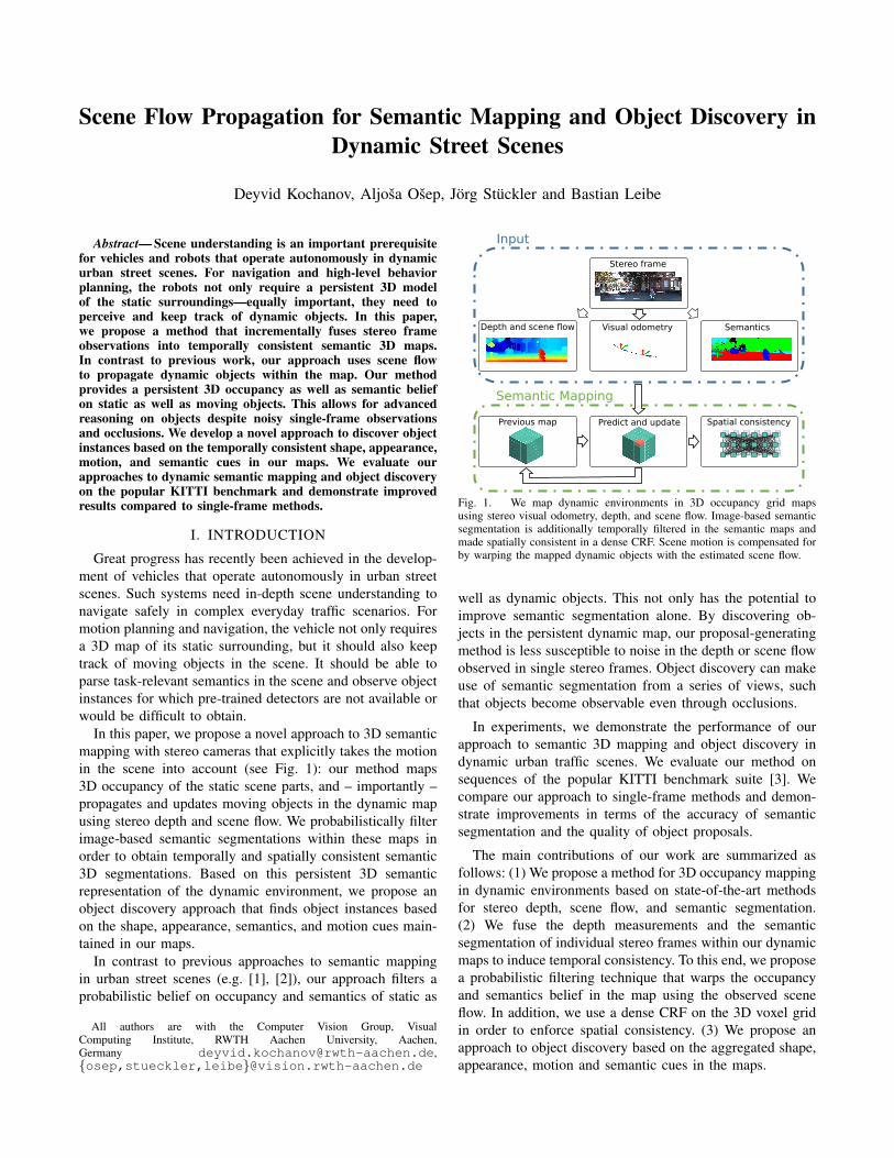
Fig. 1. We map dynamic environments in 3D occupancy grid mapsusing stereo visual odometry, depth, and scene flow. Image-based semanticsegmentation is additionally temporally filtered in the semantic maps andmade spatially consistent in a dense CRF. Scene motion is compensated forby warping the mapped dynamic objects with the estimated scene flow.

well as dynamic objects. This not only has the potential to

improve semantic segmentation alone. By discovering ob-

jects in the persistent dynamic map, our proposal-generating

method is less susceptible to noise in the depth or scene flow

observed in single stereo frames. Object discovery can make

use of semantic segmentation from a series of views, such

that objects become observable even through occlusions.

In experiments, we demonstrate the performance of our

approach to semantic 3D mapping and object discovery in

dynamic urban traffic scenes. We evaluate our method on

sequences of the popular KITTI benchmark suite [3]. We

compare our approach to single-frame methods and demon-

strate improvements in terms of the accuracy of semantic

segmentation and the quality of object proposals.

The main contributions of our work are summarized as

follows: (1) We propose a method for 3D occupancy mapping

in dynamic environments based on state-of-the-art methods

for stereo depth, scene flow, and semantic segmentation.

(2) We fuse the depth measurements and the semantic

segmentation of individual stereo frames within our dynamic

maps to induce temporal consistency. To this end, we propose

a probabilistic filtering technique that warps the occupancy

and semantics belief in the map using the observed scene

flow. In addition, we use a dense CRF on the 3D voxel grid

in order to enforce spatial consistency. (3) We propose an

approach to object discovery based on the aggregated shape,

appearance, motion and semantic cues in the maps.

II. RELATED WORK

Recent trends in the development of autonomous vehicles

and robots have fuelled research in semantic mapping and

scene understanding. Simultaneous localization and mapping

in urban street scenes with vision sensors has attracted much

attention in recent years. Current state-of-the-art methods

such as ORB-SLAM [4] or LSD-SLAM [5], [6] demon-

strate consistent large-scale trajectory estimation and 3D

reconstruction. While these methods can cope with a limited

number of moving objects as outliers to the SLAM process,

they are inherently designed for static environments. Only

few SLAM methods have been proposed that explicitly

distinguish between the static parts of the environment and

dynamic objects (e.g. SLAMMOT [7], [8], or [9]). In the

indoor RGB-D SLAM domain, KinectFusion [10] and point-

based fusion techniques [11] have been proposed that can

separate dynamic parts from the static background and ex-

clude them from tracking and mapping. Recently, Newcombe

et al. [12] propose DynamicFusion, a SLAM method that

takes non-rigid motion in a small-scale scene into account

to map a canonical shape model of the deforming object.

None of the aforementioned methods incorporates scene

semantics such as the categorization of surfaces into car,

building or road, which is often argued to be an important

aspect in scene understanding. Approaches in this line of

research can be distinguished by the way the semantic seg-

mentation is obtained and how this information is integrated

and made temporally and spatially consistent in a global map.

Koppula et al. [13] investigate semantic mapping using RGB-

D sensors in indoor scenes. They label the 3D points in an

aggregated point cloud map and impose a Markov random

field model on the points with appearance and geometric fea-

tures. Hermans et al. [14] also semantically label a 3D point

cloud map which they obtain using RGB-D visual odometry.

Their approach, however, first segments individual RGB-D

images with a random forest classifier and probabilistically

filters the soft labelling of the random forest in the 3D

points. A dense 3D conditional random field (CRF) enforces

spatial consistency on the semantic labels of the point cloud

map. The semantic SLAM approach by Stuckler et al. [15]

filters the semantic segmentation from an RF classifier in

multi-resolution surfel maps, while concurrently performing

keyframe-based SLAM based on the map representation.

Differently to our method, the aforementioned approaches

assume the environment to remain static during the semantic

mapping process.

Semantic mapping in outdoor street scenes is considered

by Sengupta et al. [16]. In this work, stereo images are first

segmented into object classes with a CRF approach. In a

second CRF stage, the image-based semantic segmentation

is fused on a ground plane projection. In [1], Sengupta et

al. fuse a CRF semantic labeling of stereo images in a 3D

point cloud map. Floros and Leibe [17] use a higher-order

CRF in order to enforce a consistent semantic labelling of 3D

points that backproject into individual image-based semantic

segmentations. Valentin et al. [18] use a triangle mesh to

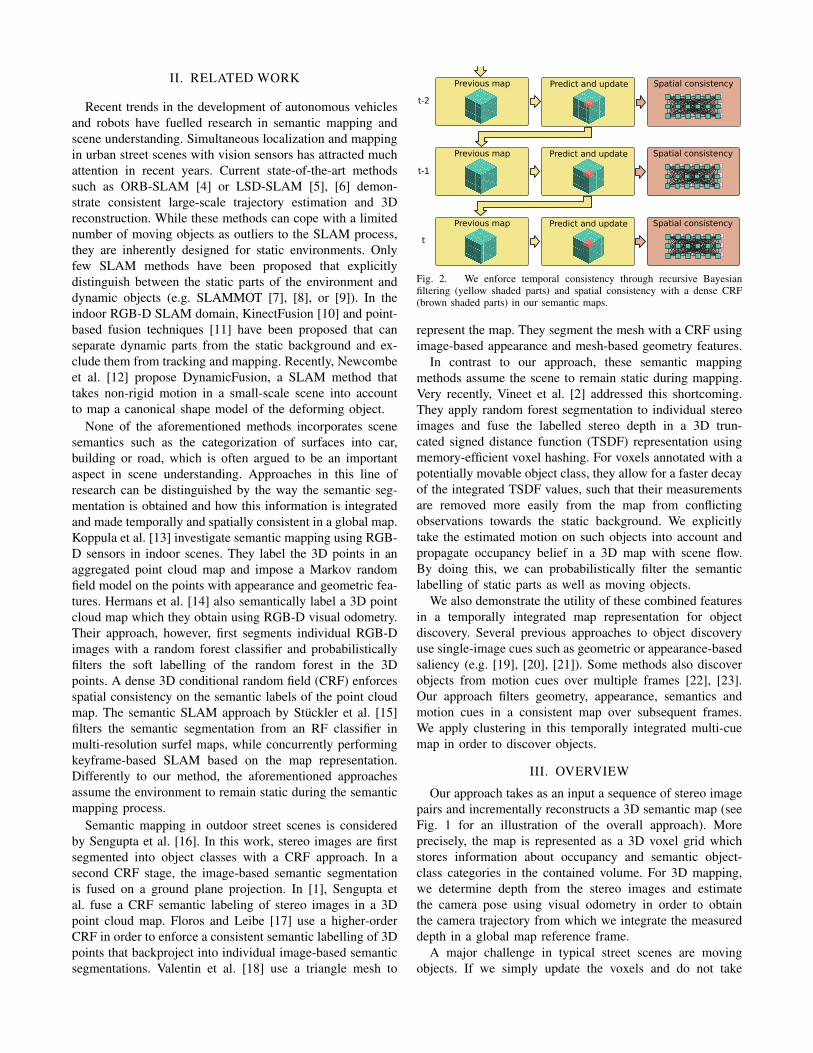
Fig. 2. We enforce temporal consistency through recursive Bayesianfiltering (yellow shaded parts) and spatial consistency with a dense CRF(brown shaded parts) in our semantic maps.

represent the map. They segment the mesh with a CRF using

image-based appearance and mesh-based geometry features.

In contrast to our approach, these semantic mapping

methods assume the scene to remain static during mapping.

Very recently, Vineet et al. [2] addressed this shortcoming.

They apply random forest segmentation to individual stereo

images and fuse the labelled stereo depth in a 3D trun-

cated signed distance function (TSDF) representation using

memory-efficient voxel hashing. For voxels annotated with a

potentially movable object class, they allow for a faster decay

of the integrated TSDF values, such that their measurements

are removed more easily from the map from conflicting

observations towards the static background. We explicitly

take the estimated motion on such objects into account and

propagate occupancy belief in a 3D map with scene flow.

By doing this, we can probabilistically filter the semantic

labelling of static parts as well as moving objects.

We also demonstrate the utility of these combined features

in a temporally integrated map representation for object

discovery. Several previous approaches to object discovery

use single-image cues such as geometric or appearance-based

saliency (e.g. [19], [20], [21]). Some methods also discover

objects from motion cues over multiple frames [22], [23].

Our approach filters geometry, appearance, semantics and

motion cues in a consistent map over subsequent frames.

We apply clustering in this temporally integrated multi-cue

map in order to discover objects.

III. OVERVIEW

Our approach takes as an input a sequence of stereo image

pairs and incrementally reconstructs a 3D semantic map (see

Fig. 1 for an illustration of the overall approach). More

precisely, the map is represented as a 3D voxel grid which

stores information about occupancy and semantic object-

class categories in the contained volume. For 3D mapping,

we determine depth from the stereo images and estimate

the camera pose using visual odometry in order to obtain

the camera trajectory from which we integrate the measured

depth in a global map reference frame.

A major challenge in typical street scenes are moving

objects. If we simply update the voxels and do not take

motion into account, moving objects would leave trails of

erroneous occupancy belief in the map. We thus compute

scene flow, i.e., the 3D motion of each stereo image pixel,

in order to take motion into account. We accumulate the

flow in the voxels and use it to propagate the occupancy

and semantic belief on dynamic objects within the map. To

this end, we propose an efficient grid warping procedure

which also takes the uncertainty of the flow measurements

into account.

At every time step, we also extract semantic information

from the stereo images and filter it in the map through time.

We compute an image-level semantic segmentation which

results in a probabilistic per-pixel label assignment. Using

the label distribution, we perform a Bayesian update on the

semantic category of the corresponding voxel.

This method of updating the map allows us to integrate

information from multiple frames (see Fig. 2). A main

advantage of the integration over time is the ability to

enforce temporal consistency in the semantic labeling and

3D reconstruction. We additionally employ a probabilistic

3D Voxel-CRF model to enforce spatial consistency of the

semantic labels. Note that we filter the distribution over

semantic labels in the temporal domain and only apply a CRF

on top of the accumulated voxel grid to obtain the most likely

explanation of accumulated measurements in each frame.

This explanation may change in future frames in the presence

of new evidence.

Finally, we describe our object proposal generation method

that builds on the reconstructed 3D semantic map. Our

method uses a clustering algorithm on the aggregated maps

that groups voxels into objects proposals based on shape,

appearance, motion and semantic cues.

IV. SEMANTIC MAPPING IN DYNAMIC STREET SCENES

A. Stereo Depth and Motion Estimation

Based on the stereo frames we estimate visual odometry,

image depth and scene flow, which we will further use in our

semantic mapping pipeline. We build on the stereo visual

odometry proposed by Geiger et al. [24]. It is a sparse

keypoint-based method which is specifically designed for

the stereo setup and the street scenes typical to automotive

scenarios.

Given two stereo pairs, captured at consecutive time steps,

scene flow methods estimate the 3D motion at each pixel in

the scene. In our experiments we used the state-of-the-art

scene flow method by Vogel et al. [25]. For each pixel in

the images the method computes both depth and 3D flow

concurrently. It approximates the scene with a set of planar

segments in superpixels for which a rigid motion towards

a reference stereo frame is determined. Note that we can

easily subtract the scene-flow induced by the ego-motion of

the camera using the visual odometry estimate.

B. Semantic Stereo Image Segmentation

Semantic segmentation aims at mapping the pixels in

the stereo images to one of several category labels l ∈{1, . . . , L} such as car, road or building. We apply the

semantic segmentation approach proposed in [26] which is

based on classifying supervoxels using a random forest clas-

sifier. Instead of making a hard decision on each supervoxel,

it provides a probabilistic classification output in the form

of a label distribution. This way, the uncertain decisions

can be filtered temporally and be incorporated as per-voxel

label evidence in a probabilistic spatial CRF model. We use

the image and point cloud to compute the following 150-

dim. features for each supervoxel within the random forest

classifier as in [26].

1) Appearance Features: These features capture the color

and texture statistics of the supervoxels. For the color, we

compute a 10-bin color histogram in the CIELab color space

for each channel. In addition, we determine the mean and

covariance of the gradients in each channel. Finally, we add

a histogram of textons computed as described in [27].

2) Density Features: This shape feature describes the den-

sity of 3D points around the supervoxel They are computed

by estimating a ground plane and discretizing the point

cloud into a grid with 3 height bins, using 3 different grid

resolutions to capture context at different scales. We project

each centroid of the supervoxels to the grid and examine its

4-neighbourhood at its height.

3) Spectral Features: We compute this second type of

shape features from the eigenvectors and the eigenvalues of

the covariance matrix of the points in the supervoxel. Look-

ing at eigenvalues, we can quantify pointness, linearness,

surfaceness and curvature [28] of the segment. We compute

the surface normal from the eigenvectors and measure the

orientation of the supervoxel as the angle between the surface

normal and the ground plane normal.

4) Locational Features: The relative location of a super-

voxel in the scene is encoded by the distance of its centroid

to the ground plane, its distance from the camera, and the

horizontal angle between the optical axis and the ray from

the focal point to the supervoxel’s centroid.

C. Mapping of Dynamic Scenes

We now arrive at our algorithm for 3D mapping of

occupancy and semantics from a moving stereo camera in a

dynamic (street) scene. The main challenge in this setting is

to construct a mapping method which can effectively account

for the motion of objects. In each time step t, our algorithm

receives the current stereo frame It. From this image, we

extract a depth map dt and a semantic segmentation st which

we summarize in the observation xt = {dt, st}. Semantic

segmentation yields a probability distribution p(lu | It) on

the labelling of each image pixel u.

In addition to these single-frame measurements, visual

odometry provides us with the pose pt of the camera in

the world frame at time t. Piece-wise rigid scene flow ft is

estimated from the last frame It−1 to the current frame It,

which we compensate for the ego-motion of the camera

with the visual odometry estimate. We summarize the visual

odometry and scene flow estimates up to time t by Pt

and F t, respectively. In analogy, we write X t to denote the

series of observations x0, . . . , xt.

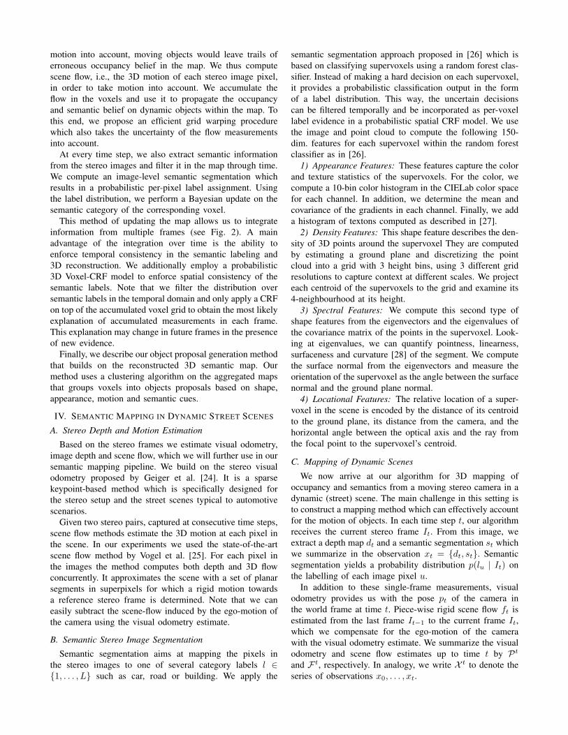
Fig. 3. Voxel map representation. Top: Corresponding image from theKITTI benchmark. Middle: Voxel map for the stereo frame, colorized withthe average color of image pixels in the voxel. Bottom: Average voxel flow(red lines, voxel centers depicted as colored disks).

1) Map Representation: We represent our map with vox-

els vj using sparse and memory-efficient voxel hashing [29].

Each voxel of size 0.1m×0.1m×0.1m maintains a distribu-

tions on occupancy p(oj | Xt,Pt,F t) and semantic labelling

p(lj | Xt,Pt,F t).

2) Probabilistic Mapping: The stereo images provide ob-

servations of voxel occupancy and semantic labelling, which

we transform from the camera frame to the world frame using

the visual odometry estimate. Scene dynamics is observed by

ego-motion-compensated scene flow. Under this model, the

occupancy and semantic belief in each voxel yt,j is updated

in a recursive Bayesian filtering scheme,

p(yt,j | Xt,F t,Pt) =

η p(xt | yt,j , pt) p(yt,j | Xt−1,F t,Pt), (1)

where η is a normalization factor. In the following, we will

drop the dependency on the visual odometry estimates Pt

for brevity.

The filter decomposes into a prediction and a correction

step. The prediction step applies a state transition model

and warps the voxel map based on the scene flow. A

subsequent correction update step incorporates the image-

based depth and semantic observations into the map. For

efficient integration of the stereo image-based observations,

we first accumulate the occupancy, semantics, and scene flow

measurements in a local map. This local map is aligned with

the grid of the temporally integrated map. Fig. 3 shows an

example of a local measurement map mt generated from a

stereo frame.

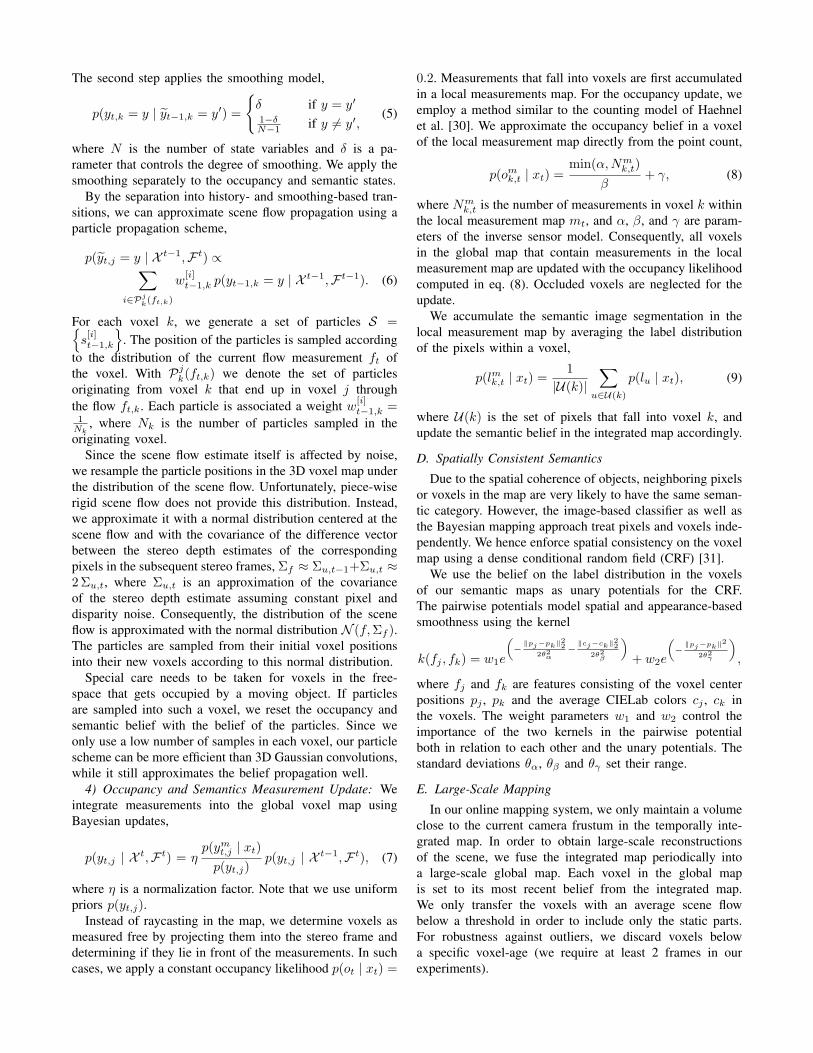
0 2 4 6 8 10 12 14

Fig. 4. Voxel-age (color-coded) in frames 1, 10, and 15 of the KITTItracking sequence 00. Voxel-age corresponds to the number of frames inwhich the voxel was updated. Remarkably, due to scene flow propagation,voxels on dynamic objects exhibit similar ageing like the static parts (best

viewed in color).

3) Dynamic Map Prediction: In the prediction step, we

determine the distribution

p(yt,j | Xt−1,F t) =

∑

k

∑

y

p(yt,j | yt−1,k = y, ft,k)

p(yt−1,k = y | X t−1,F t−1), (2)

by propagating the occupancy and label beliefs in the voxels

from the last time step based on the current scene flow

estimate. Note that we model occupancy and label belief

as stochastically independent, such that we can process both

modalities in separate Bayesian filters.

Clearly, the estimated scene flow and the imposed model

assumptions are not fully satisfied in a real setting. Hence,

the state transition should also induce additional uncertainty

on the occupancy and label belief. We incorporate this by

approximating the state transition model with two model

terms

p(yt,j | Xt−1,F t) =

∑

y

p(yt,j | yt,j = y) p(yt,j = y | X t−1,F t), (3)

where p(yt,j | yt,j) now smoothes the occupancy and label

distribution in a voxel. The propagation then splits into two

separate processes: In a first step, we propagate the belief

from the previous frame with the scene flow to obtain an

intermediate distribution on yt,j ,

p(yt,j = y | X t−1,F t) =∑

k

p(yt,j = y | yt−1,k = y, ft,k)

p(yt−1,k = y | X t−1,F t−1). (4)

The second step applies the smoothing model,

p(yt,k = y | yt−1,k = y′) =

{δ if y = y′

1−δN−1 if y 6= y′,

(5)

where N is the number of state variables and δ is a pa-

rameter that controls the degree of smoothing. We apply the

smoothing separately to the occupancy and semantic states.

By the separation into history- and smoothing-based tran-

sitions, we can approximate scene flow propagation using a

particle propagation scheme,

p(yt,j = y | X t−1,F t) ∝∑

i∈Pj

k(ft,k)

w[i]t−1,k p(yt−1,k = y | X t−1,F t−1). (6)

For each voxel k, we generate a set of particles S ={s[i]t−1,k

}. The position of the particles is sampled according

to the distribution of the current flow measurement ft of

the voxel. With Pjk(ft,k) we denote the set of particles

originating from voxel k that end up in voxel j through

the flow ft,k. Each particle is associated a weight w[i]t−1,k =

1Nk

, where Nk is the number of particles sampled in the

originating voxel.

Since the scene flow estimate itself is affected by noise,

we resample the particle positions in the 3D voxel map under

the distribution of the scene flow. Unfortunately, piece-wise

rigid scene flow does not provide this distribution. Instead,

we approximate it with a normal distribution centered at the

scene flow and with the covariance of the difference vector

between the stereo depth estimates of the corresponding

pixels in the subsequent stereo frames, Σf ≈ Σu,t−1+Σu,t ≈2Σu,t, where Σu,t is an approximation of the covariance

of the stereo depth estimate assuming constant pixel and

disparity noise. Consequently, the distribution of the scene

flow is approximated with the normal distribution N (f,Σf ).The particles are sampled from their initial voxel positions

into their new voxels according to this normal distribution.

Special care needs to be taken for voxels in the free-

space that gets occupied by a moving object. If particles

are sampled into such a voxel, we reset the occupancy and

semantic belief with the belief of the particles. Since we

only use a low number of samples in each voxel, our particle

scheme can be more efficient than 3D Gaussian convolutions,

while it still approximates the belief propagation well.

4) Occupancy and Semantics Measurement Update: We

integrate measurements into the global voxel map using

Bayesian updates,

p(yt,j | X t,F t) = ηp(ymt,j | xt)

p(yt,j)p(yt,j | X t−1,F t), (7)

where η is a normalization factor. Note that we use uniform

priors p(yt,j).Instead of raycasting in the map, we determine voxels as

measured free by projecting them into the stereo frame and

determining if they lie in front of the measurements. In such

cases, we apply a constant occupancy likelihood p(ot | xt) =

0.2. Measurements that fall into voxels are first accumulated

in a local measurements map. For the occupancy update, we

employ a method similar to the counting model of Haehnel

et al. [30]. We approximate the occupancy belief in a voxel

of the local measurement map directly from the point count,

p(omk,t | xt) =min(α,Nm

k,t)

β+ γ, (8)

where Nmk,t is the number of measurements in voxel k within

the local measurement map mt, and α, β, and γ are param-

eters of the inverse sensor model. Consequently, all voxels

in the global map that contain measurements in the local

measurement map are updated with the occupancy likelihood

computed in eq. (8). Occluded voxels are neglected for the

update.

We accumulate the semantic image segmentation in the

local measurement map by averaging the label distribution

of the pixels within a voxel,

p(lmk,t | xt) =1

|U(k)|

∑

u∈U(k)

p(lu | xt), (9)

where U(k) is the set of pixels that fall into voxel k, and

update the semantic belief in the integrated map accordingly.

D. Spatially Consistent Semantics

Due to the spatial coherence of objects, neighboring pixels

or voxels in the map are very likely to have the same seman-

tic category. However, the image-based classifier as well as

the Bayesian mapping approach treat pixels and voxels inde-

pendently. We hence enforce spatial consistency on the voxel

map using a dense conditional random field (CRF) [31].

We use the belief on the label distribution in the voxels

of our semantic maps as unary potentials for the CRF.

The pairwise potentials model spatial and appearance-based

smoothness using the kernel

k(fj , fk) = w1e

(

−‖pj−pk‖2

2

2θ2α−

‖cj−ck‖22

2θ2β

)

+ w2e

(

−‖pj−pk‖2

2θ2γ

)

,

where fj and fk are features consisting of the voxel center

positions pj , pk and the average CIELab colors cj , ck in

the voxels. The weight parameters w1 and w2 control the

importance of the two kernels in the pairwise potential

both in relation to each other and the unary potentials. The

standard deviations θα, θβ and θγ set their range.

E. Large-Scale Mapping

In our online mapping system, we only maintain a volume

close to the current camera frustum in the temporally inte-

grated map. In order to obtain large-scale reconstructions

of the scene, we fuse the integrated map periodically into

a large-scale global map. Each voxel in the global map

is set to its most recent belief from the integrated map.

We only transfer the voxels with an average scene flow

below a threshold in order to include only the static parts.

For robustness against outliers, we discard voxels below

a specific voxel-age (we require at least 2 frames in our

experiments).

V. OBJECT DISCOVERY IN DYNAMIC SEMANTIC MAPS

Generating object proposals from semantic maps instead

of individual images has several potential advantages. Inte-

grating semantic segmentations over time leads to a more

accurate, stable labeling. The integration of occupancy in-

formation over time significantly improves the noisy stereo

depth information present in a single frame. Finally, integra-

tion over time in a map helps us to generate proposals for

objects which may be strongly occluded in individual frames.

We propose to employ density-based spatial clustering

(DBSCAN [32]) on features extracted from the semantic

map (see. Fig. 8). DBSCAN clusters points in a feature-

space based on their distance in a bottom-up way. It starts

clustering at core points with at least Nmin number of

points in an ε-neighborhood. It expands from these points

recursively to core points within the ε-neighborhood and

includes all points within the neighborhood.

As features for each occupied voxel labelled with the

‘object’ class label, we use a concatenation of its center

position, its average color in CIELab color space, and its

average scene flow. We extract proposals at multiple scales

by varying the ε-neighborhood in a discrete range of val-

ues (ε ∈ {1.7, 1.9, 2.1, 2.3, 2.4, 2.6, 2.8, 3.0} in our experi-

ments). For each radius, we additionally vary the occupancy

thresholds θo at which voxels are considered for clustering

(we use the values θo ∈ {0.6, 0.7, 0.8, 0.85, 0.9, 0.95, 0.98}in our experiments). After computing proposals across scales,

we merge them according to their bounding box overlap in

the image domain and rank the merged proposals by the

number of the matchings.

VI. EXPERIMENTS

We evaluate our approaches to semantic mapping and

object discovery on datasets from the popular KITTI bench-

mark [3]. On the KITTI odometry dataset, we evaluate

semantic mapping based on custom dense object-class an-

notations of 200 of the images. We used the same split into

training and test set to train the random forest classifier and

to evaluate our segmentation results as in [26]. Our method

for object discovery is assessed on the tracking dataset which

comes with ground truth annotations for bounding boxes on

objects such as cars, pedestrians, and bicyclists.

Besides training the RF classifier, we also determined

the remaining parameters of our method empirically on the

training split. To find good values for the CRF parameters

we performed grid search. We ran the MAP inference using

the RF unaries and evaluated the semantic segmentation on

15 frames from our training set. This yielded the settings

w(1) = 2.5, w(2) = 1, θα = 2.5, θβ = 7 and θγ = 0.3.

A. Semantic Dynamic Mapping

We evaluate the quality of the semantic labelling in our 3D

maps using the image-based ground truth annotations on the

KITTI odometry dataset. To this end, we generate a semantic

labelling of the stereo frames from the belief contained in our

semantic maps. We directly lookup the semantic labelling

of each image pixel using its depth measurement at its

RF + CRF semantic map

recall IoU recall IoU

object 84.02 67.39 83.02 70.39

road 94.04 91.50 93.41 92.11

building 83.29 75.27 86.91 76.68

tree/bush 70.36 64.59 68.97 64.35sign/pole 4.09 3.83 1.96 1.88sky 35.84 34.43 40.91 39.75

grass/dirt 60.63 26.77 79.46 25.23

pixel avg. (< 25m) 87.71 78.25 87.99 78.55

class avg. (< 25m) 68.54 57.47 70.46 57.81

pixel avg. (all depths) 78.08 70.46 79.13 71.05

class avg. (all depths) 61.75 51.97 64.95 52.91

TABLE I

SEMANTIC SEGMENTATION RESULTS ON THE KITTI ODOMETRY

DATASET.

corresponding voxel in the map. Only if no depth is available

at a pixel, we ray-cast for the label.

Fig. 5 shows a qualitative result of our mapping approach

in a high-traffic road scene. It can be seen that the dynamic

objects are well segmented from the static parts and not

included in the large-scale map. The semantic segmentation

finds a consistent labelling of the cars and traffic signs as

objects. It also segments the larger surface categories such

as road and vegetation well.

The segmentation quality is assessed using the Pascal VOC

intersection-over-union measure (IoU [33]). We compare our

approach with a purely image-based semantic segmentation

method that applies spatial smoothing on the RF output

using the dense CRF [26]. Note that for pixels without a

valid depth, the pixel is assigned to a void class which is

accounted as false positive if it should label one of the object

classes. In Table I we report recall and IoU over all pixels,

class-wise, and by class-averages on the test set. From the

results we observe that on average the semantic informa-

tion contained in our maps clearly outperforms the single-

frame-based semantic segmentation baseline (RF+CRF). Our

method also demonstrates improvements in recall and IoU

over the single-frame-based segmentation on several object

classes with medium-sized and larger structures. Notably,

on classes which contain finer structures, image-based seg-

mentation can perform slightly better. This is likely due

to the highly noisy stereo depth that is unreliable in such

thin structures. Especially at very far distances, this renders

consistent integration of fine structures in the map difficult.

Interestingly, averaged over all classes, the improvements by

our persistent maps are stronger if we consider all depths

compared to a limited range of up to 25m (chosen as in [2]).

B. Object Discovery

For evaluating our object-instance proposal method on

the temporally integrated semantic maps, we follow the

evaluation protocol in [26]. We use the KITTI tracking

training set [3] due to the public availability of the ground-

truth annotations of object bounding boxes. Note that se-

mantic segmentation was trained on a non-overlapping set of

semantic labels and that we set the parameters of the object

Building Grass/Dirt Object Road Sky Sign/Pole Tree/Bush

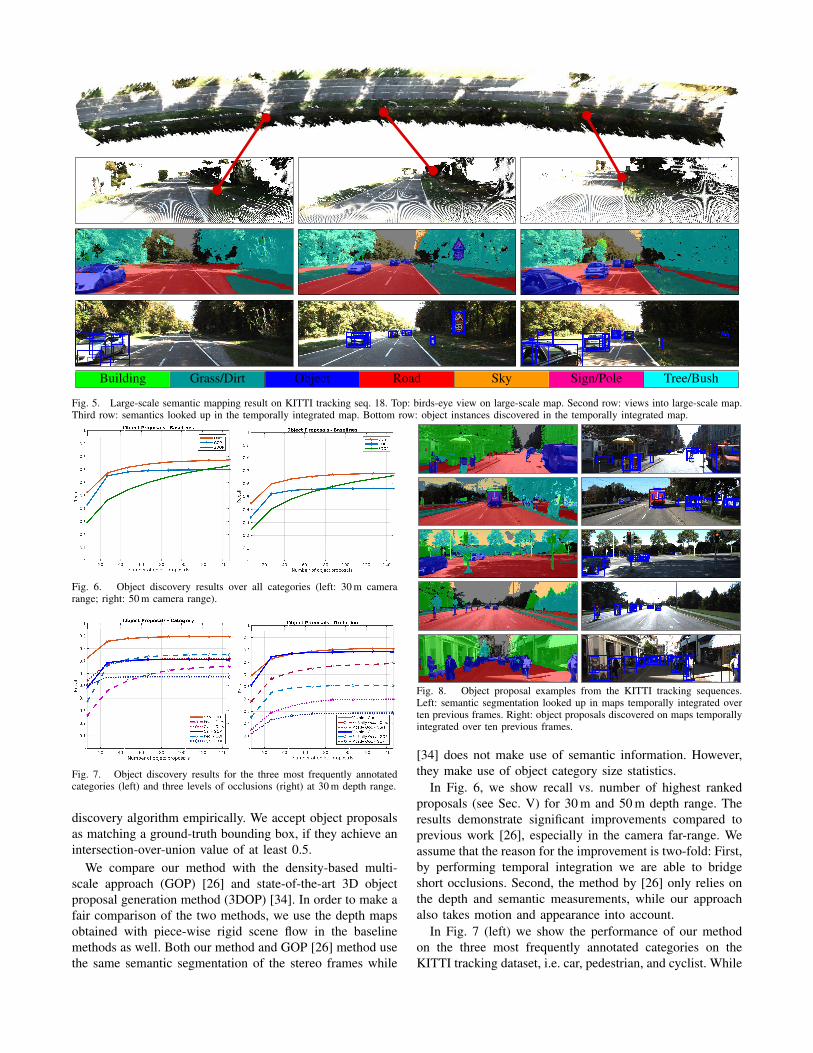
Fig. 5. Large-scale semantic mapping result on KITTI tracking seq. 18. Top: birds-eye view on large-scale map. Second row: views into large-scale map.Third row: semantics looked up in the temporally integrated map. Bottom row: object instances discovered in the temporally integrated map.

Fig. 6. Object discovery results over all categories (left: 30 m camerarange; right: 50 m camera range).

Fig. 7. Object discovery results for the three most frequently annotatedcategories (left) and three levels of occlusions (right) at 30 m depth range.

discovery algorithm empirically. We accept object proposals

as matching a ground-truth bounding box, if they achieve an

intersection-over-union value of at least 0.5.

We compare our method with the density-based multi-

scale approach (GOP) [26] and state-of-the-art 3D object

proposal generation method (3DOP) [34]. In order to make a

fair comparison of the two methods, we use the depth maps

obtained with piece-wise rigid scene flow in the baseline

methods as well. Both our method and GOP [26] method use

the same semantic segmentation of the stereo frames while

Fig. 8. Object proposal examples from the KITTI tracking sequences.Left: semantic segmentation looked up in maps temporally integrated overten previous frames. Right: object proposals discovered on maps temporallyintegrated over ten previous frames.

[34] does not make use of semantic information. However,

they make use of object category size statistics.

In Fig. 6, we show recall vs. number of highest ranked

proposals (see Sec. V) for 30 m and 50 m depth range. The

results demonstrate significant improvements compared to

previous work [26], especially in the camera far-range. We

assume that the reason for the improvement is two-fold: First,

by performing temporal integration we are able to bridge

short occlusions. Second, the method by [26] only relies on

the depth and semantic measurements, while our approach

also takes motion and appearance into account.

In Fig. 7 (left) we show the performance of our method

on the three most frequently annotated categories on the

KITTI tracking dataset, i.e. car, pedestrian, and cyclist. While

our method clearly outperforms GOP on the car and cyclist

categories, this baseline seems better suitable for detection of

individual pedestrians. This is due to the fact that pedestrians

in KITTI mostly appear in groups. Due to inaccuracies in

the scene flow estimation, occupancy beliefs in these cells

become blurred and groups are perceived as single objects.

Fig. 7 (right) compares our method with the baseline w.r.t.

the amount of occlusion on the objects. The results clearly

show that the main advantage of our method over GOP is due

to the temporal integration. Finally, Fig. 8 shows example

results obtained with our approach. It can be seen that our

method provides proposals on a wide range of generic objects

(e.g. truck, dog, traffic sign/poles, post-box etc.) and finds

them even in difficult occlusion situations (e.g. the car behind

the traffic sign in 3rd row).

VII. CONCLUSIONS

In this paper, we have proposed a novel approach to 3D

semantic mapping and object discovery in dynamic street

scenes. We use scene flow to propagate occupancy and

semantic belief in the map. In this way, our maps maintain a

temporally consistent semantic belief not only on the static

parts of the environment as in previous approaches, but also

on dynamic objects. Based on our map representation, we

develop an object discovery approach that is less susceptible

to occlusions and noisy observations in single stereo frames.

We develop our method as an important building-block

for our future research in detailed 3D scene understanding

in the close camera range. Potential next steps will be the

tracking of discovered objects over time and to reason about

their occupancy in separate, object-centric voxel grids.

ACKNOWLEDGEMENTS

This work was funded by ERC Starting Grant project CV-

SUPER (ERC-2012-StG-307432). We would like to thank

Alexander Hermans for helpful discussions.

REFERENCES

[1] S. Sengupta, E. Greveson, A. Shahrokni, and P. Torr, “Urban 3Dsemantic modelling using stereo vision,” in Proc. of IEEE ICRA, 2013.

[2] V. Vineet, O. Miksik, M. Lidegaard, M. Niessner, S. Golodetz,V. Prisacariu, O. Kahler, D. Murray, S. Izadi, P. Peerez, and P. Torr,“Incremental dense semantic stereo fusion for large-scale semanticscene reconstruction,” in Proc. of IEEE ICRA, 2015, pp. 75–82.

[3] A. Geiger, P. Lenz, and R. Urtasun, “Are we ready for AutonomousDriving? The KITTI Vision Benchmark Suite,” in Proc. of IEEE

CVPR, 2012.

[4] R. Mur-Artal, J. Montiel, and J. Tardos, “ORB-SLAM: A versatile andaccurate monocular SLAM system,” IEEE Trans. on Robotics, vol. 31,no. 5, pp. 1147–1163, 2015.

[5] J. Engel, T. Schops, and D. Cremers, “LSD-SLAM: Large-scale directmonocular SLAM,” in Proc. of ECCV, 2014.

[6] J. Engel, J. Stuckler, and D. Cremers, “Large-scale direct SLAM withstereo cameras,” in Proc. of IEEE/RSJ IROS, 2015.

[7] C.-C. Wang, C. Thorpe, and S. Thrun, “Online simultaneous local-ization and mapping with detection and tracking of moving objects:Theory and results from a ground vehicle in crowded urban areas,” inProc. of IEEE ICRA, 2003.

[8] E. Einhorn and H.-M. Gross, “Generic NDT mapping in dynamicenvironments and its application for lifelong SLAM,” Robotics and

Autonomous Systems, vol. 69, pp. 28 – 39, 2015.

[9] R. Danescu, C. Pantilie, F. Oniga, and S. Nedevschi, “Particle gridtracking system stereovision based obstacle perception in drivingenvironments,” IEEE Intelligent Transportation Systems Magazine,vol. 4, no. 1, pp. 6–20, 2012.

[10] R. A. Newcombe, S. Izadi, O. Hilliges, D. Molyneaux, D. Kim, A. J.Davison, P. Kohli, J. Shotton, S. Hodges, and A. W. Fitzgibbon,“KinectFusion: Real-time dense surface mapping and tracking.” inISMAR, 2011, pp. 127–136.

[11] M. Keller, D. Lefloch, M. Lambers, S. Izadi, T. Weyrich, and A. Kolb,“Real-time 3d reconstruction in dynamic scenes using point-basedfusion,” in Proc of Int. Conf. on 3D Vision (3DV), 2013, pp. 1–8.

[12] R. A. Newcombe, D. Fox, and S. M. Seitz, “DynamicFusion: Recon-struction and tracking of non-rigid scenes in real-time,” in Proc. of

IEEE CVPR, 2015.[13] H. S. Koppula, A. Anand, T. Joachims, and A. Saxena, “Semantic

labeling of 3D point clouds for indoor scenes,” in Proc. of NIPS,2011.

[14] A. Hermans, G. Floros, and B. Leibe, “Dense 3D semantic mappingof indoor scenes from RGB-D images,” in Proc. of IEEE ICRA, 2014.

[15] J. Stuckler, B. Waldvogel, H. Schulz, and S. Behnke, “Dense real-time mapping of object-class semantics from RGB-D video,” J. of

Real-Time Image Processing, vol. 10, no. 4, pp. 599–609, 2013.[16] S. Sengupta, P. Sturgess, L. Ladicky, and P. Torr, “Automatic dense

visual semantic mapping from street-level imagery,” in Proc. of

IEEE/RSJ IROS, 2012.[17] G. Floros and B. Leibe, “Joint 2d-3d temporally consistent semantic

segmentation of street scenes,” in Proc. of IEEE CVPR, 2012.[18] J. Valentin, S. Sengupta, J. Warrell, A. Shahrokni, and P. Torr, “Mesh

based semantic modelling for indoor and outdoor scenes,” in Proc. of

IEEE CVPR, 2013, pp. 2067–2074.[19] D. Mitzel and B. Leibe, “Taking Mobile Multi-Object Tracking to the

Next Level: People, Unknown Objects, and Carried Items,” in Proc.

of ECCV, 2012.[20] A. Karpathy, S. Miller, and L. Fei-Fei, “Object discovery in 3D scenes

via shape analysis,” in Proc. of IEEE ICRA, 2013.[21] G. M. Garcia, E. Potapova, T. Werner, M. Zillich, M. Vincze, and

S. Frintrop, “Saliency-based object discovery on RGB-D data with alate-fusion approach,” in Proc. of IEEE ICRA, 2015.

[22] A. Bewley, V. Guizilini, F. Ramos, and B. Upcroft, “Online Self-Supervised Multi-Instance Segmentation of Dynamic Objects,” inProc. of IEEE ICRA, 2014.

[23] T. Scharwachter, M. Enzweiler, U. Franke, and S. Roth, “Stixmantics:A Medium-Level Model for Real-Time Semantic Scene Understand-ing,” in Proc. of ECCV, 2014.

[24] A. Geiger, J. Ziegler, and C. Stiller, “StereoScan: Dense 3d Recon-struction in Real-time,” in Intel. Vehicles Symp.’11, 2011.

[25] C. Vogel, K. Schindler, and S. Roth, “Piecewise rigid scene flow,” inProc. of IEEE Int. Conf. on Computer Vision (ICCV), 2013.

[26] A. Osep, A. Hermans, F. Engelmann, D. Klostermann, , M. Math-ias, and B. Leibe, “Multi-scale object candidates for generic objecttracking in street scenes,” in Proc. of IEEE ICRA, 2016.

[27] J. Shotton, J. M. Winn, C. Rother, and A. Criminisi, “TextonBoostfor Image Understanding: Multi-Class Object Recognition and Seg-mentation by Jointly Modeling Texture, Layout, and Context,” IJCV,vol. 81, no. 1, pp. 2–23, 2009.

[28] D. Munoz, N. Vandapel, and M. Hebert, “Onboard Contextual Classifi-cation of 3-D Point Clouds with Learned High-order Markov RandomFields,” in Proc. of IEEE ICRA, 2009.

[29] M. Nießner, M. Zollhofer, S. Izadi, and M. Stamminger, “Real-time 3Dreconstruction at scale using voxel hashing,” ACM Trans. Graphics,2013.

[30] D. Hahnel, “Mapping with mobile robots,” Ph.D. dissertation, Univer-sity of Freiburg, 2005.

[31] P. Krahenbuhl and V. Koltun, “Efficient Inference in Fully ConnectedCRFs with Gaussian Edge Potentials,” in Proc. of NIPS, 2011.

[32] M. Ester, H.-P. Kriegel, J. Sander, and X. Xu, “A density-basedalgorithm for discovering clusters in large spatial databases withnoise,” in Proc. of Int. Conf. on Knowledge Discovery and Data

Mining (KDD), 1996.[33] M. Everingham, L. V. Gool, C. K. I. Williams, J. Winn, and A. Zisser-

man, “The pascal visual object classes (voc) challenge,” IJCV, vol. 88,no. 2, pp. 303–308, 2009.

[34] X. Chen, K. Kundu, Z. Zhang, H. Ma, S. Fidler, and R. Urtasun,“Monocular 3d object detection for autonomous driving,” in Proc. of

IEEE CVPR, 2016.