Abstract In this paper, we study thermal-constrained hard real-time systems, wherereal-time guarantees must be met without exceeding safe temperature levels withinthe processor. Dynamic speed scaling is one of the major techniques to manage powerso as to maintain safe temperature levels. As example, we adopt a reactive speed con-trol technique in our work. We design an extended busy-period analysis methodologyto perform schedulability analysis for general task arrivals under reactive speed con-trol with First-In-First-Out (FIFO), Static-Priority (SP), and Earliest-Deadline-First(EDF) scheduling. As a special case, we obtain a closed-form formula for the worst-case response time of jobs under the leaky-bucket task arrival model. Our data showhow reactive speed control can decrease the worst-case response time of tasks incomparison with any constant-speed scheme.
With the rapidly increasing power density in processors the problem of thermal man-agement in systems is becoming acute. Methods to manage heat to control its dissipa-tion have been gaining much attention by researchers and practitioners. Techniquesare being investigated for thermal control both at design time through appropriatepackaging and active heat dissipation mechanisms, and at run time through variousforms of dynamic thermal management (DTM) (e.g., Brooks and Martonosi 2001).
Thermal management through packaging (that improves airflow, for example) andactive heat dissipation is very expensive. Tiwari et al. (1998) for example show howthe incremental packaging cost per additional Watt becomes very high for processorsabove 35–40 W power dissipation. A recent technology roadmap of the Semiconduc-tor Industry Association (ITRS05 2005) predicts that packaging will become increas-ingly challenging in the near future, due to the high levels of peak power involved andthe extremely high power density in emerging systems-in-package. In addition, formany high-performance embedded systems the packaging requirements and operat-ing environments render expensive and bulky packaging solutions inappropriate.
A number of DTM approaches to control the temperature at run time have beenproposed, ranging from clock throttling to dynamic voltage scaling (DVS) to in-chipload balancing:
– Many processors use Clock Throttling (e.g., Rotem et al. 2004) or Clock Gating(Skadron et al. 2003) to stall the clock and so allow the processor to cool duringthermal overload.
– DVS (Brooks and Martonosi 2001) is used in a variety of modern processor tech-nologies and allows to switch between different frequency and voltage operatingpoints at run time in response to the current thermal situation. In the Enhanced In-tel SpeedStep mechanism in the Pentium M processor, for example, a low-poweroperating point is reached in response to a thermal trigger by first reducing thefrequency (within a few microseconds) and then reducing the voltage (at a rate ofone mV per microsecond; Rotem et al. 2004).
– A number of architecture-level mechanisms for thermal control have been pro-posed that turn off components inside the processor in response to thermal over-load. Skadron et al. (2003) for example argue that the microarchitecture shoulddistribute the workload in response to the thermal situation by taking advantage ofinstruction-level parallelism. The performance penalty caused by this “local gat-ing” would not be excessive. On a coarser level, the Pentium Core Duo Architec-ture allows the OS or the BIOS to disable one of the cores by putting it into sleepmode (Gochman et al. 2006).
As high-performance embedded systems become increasingly thermally-con-strained, the question of how the thermal behavior of the system and the thermalcontrol mechanisms affect real-time guarantees must be addressed. In this paper wedescribe schedulability analysis techniques in thermally-constrained hard real-timesystems, where deadline constraints for tasks have to be balanced against tempera-ture constraints of the system.
162 Real-Time Syst (2010) 46: 160–188
Both in research and practice, dynamic speed control1 is one of the major tech-niques to control the temperature. Dynamic speed scaling allows for a trade-off be-tween these two performance metrics: To meet the deadline constraint, we run theprocessor at a higher speed; To maintain the safe temperature levels, we run theprocess at a lower speed.
There is some recent work on dynamic speed scaling techniques to control tem-perature. For example, in Srinivasan and Adve (2003), a predictive DTM algorithmwas designed to improve the performance of multimedia applications. In Cohen etal. (2003), Rao et al. (2006), optimal speed profiles were derived to achieve high re-source utilization. This work focuses on improving resource utilization rather than onproviding real-time guarantees, which is the focus of this paper. Zhang and Chatha(2007) address the knapsack problem for a given execution sequence of jobs by as-signing discrete frequency/voltage states. They prove that the problem is NP-hard andproceed to formulate a pseudo-polynomial optimal speed assignment algorithm anda polynomial time approximation algorithm.
The work on dynamic speed scaling techniques to control temperature in real-time systems was initiated in Bansal et al. (2004) and further investigated in Bansaland Pruhs (2005). Both Bansal et al. (2004) and Bansal and Pruhs (2005) focus ononline algorithms in real-time systems, where the scheduler learns about a task onlyat its release time. In contrast, in our work we assume a predictive task model (e.g.,periodic tasks) and so allow for design-time schedulability analysis. In Ferreira et al.(2006), a thermal model is presented that is capable of modeling cooling faults suchas CPU fan or case fan failures and load-balancing algorithms were design based onthis model. This work is complementary to ours.
We distinguish between proactive and reactive speed scaling schemes. When-ever the temperature model is known, the scheduler could in principle use a proac-tive speed-scaling approach, where—similarly to a non-work-conserving scheduler—resources are preserved for future use. In this paper, we limit ourselves to re-active schemes, and propose a simple reactive speed scaling technique for theprocessor, which will be discussed in Sect. 2. We focus on reactive schemes pri-marily because they are simple to integrate with current processor capabilitiesthrough existing power control frameworks such as the Advanced Configuration andPower Interface (ACPI) power control framework (ACPI 2010; Sanchez et al. 1997;Rotem et al. 2004).
In order to provide timing guaranteed services for real-time tasks, schedulabilityanalysis is needed. Unfortunately, traditional schedulability analysis will not workunder thermal-aware design. In traditional schedulability analysis, we could targeton jobs only in a busy period (before and after that the processor is idle) becausethe behavior of jobs in different busy periods do not affect each other (Liu 2000).However, in thermal-aware design, it becomes difficult to separate the execution ofjobs in a busy period from the interference by the execution of jobs in an earlierbusy period because the speed of the processor is triggered by the thermal behaviorand varies over time under the DTM scheme. To tackle this issue, we introduce an
1At the risk of overly generalizing, we use the term “dynamic speed control” to subsume dynamic voltagescaling or dynamic frequency scaling.
Real-Time Syst (2010) 46: 160–188 163
extended busy-period analysis methodology. In Wang and Bettati (2008), we performschedulability analysis under reactive speed scaling for identical-period tasks. In thispaper, we extend it to general task arrivals with First-In-First-Out (FIFO), Static-Priority (SP), and Earliest-Deadline-First (EDF) scheduling.
The rest of the paper is organized as follows. In Sect. 2, we introduce the thermalmodel, the speed scaling schemes, and the task model and the scheduling algorithms.After discussing the thermal interference on schedulability analysis in Sect. 3, we de-sign the extended busy-period analysis methodology to perform schedulability analy-sis for FIFO, SP, and EDF scheduling algorithms in Sects. 4, 5, and 6 respectively. Wemeasure the response time performance for tasks under each scheduling algorithm inSect. 7. Finally, we conclude our work with final remarks and give an outlook onfuture work in Sect. 8.
2 Models
2.1 Power model
The power consumption P is contributed by the following two main sources:
– The dynamic power consumption PD mainly resulting from the charging and dis-charging of gates on the circuits. The dynamic power consumption could be mod-elled as a convex function of the processor speed such as the dynamic power con-sumption in CMOS processors (Rabaey and Chandrakasan 2002): PD = Cef V 2
dds,
where s = κv(Vdd−Vt )
2
Vddis defined as the processor speed.2 We can further sim-
plify the formula of the dynamic power consumption as PD = β0sα , where β0
and α ≤ 3 are constants. Usually, it is assumed that α = 3 (Bansal et al. 2004;Bansal and Pruhs 2005).
– The leakage power consumption PL mainly resulting from leakage current. Theleakage power consumption function of the system could be modelled as a non-negative constant when leakage power consumption is irrelevant to the tempera-ture (Xu et al. 2005; Jian-Jia et al. 2007). When the leakage power consumption isrelated to the temperature, it could be approximately modelled by a linear functionof the temperature (Chantem et al. 2008). Hence, the leakage power consumptionis as follows: PL = β1T + β2, where T is the temperature and β1 and β2 are con-stants.
In this paper, we use the following formula as the overall power consumption
P = PD + PL = β0sα + β1T + β2. (1)
The power consumption P = P(t), the speed s = s(t) and the temperature T = T (t)
are all functions of time t .
2Cef ,Vt ,Vdd , and κv denote the effective switch capacitance, the threshold voltage, the supply voltage,and a hardware-design-specific constant, respectively. Vdd ≥ Vt ≥ 0; κv,Cef > 0.
164 Real-Time Syst (2010) 46: 160–188
2.2 Thermal model
A wide range of increasingly sophisticated thermal models for integrated circuitshave been proposed in the last few years. Some are comparatively simple, chip-widemodels, such as developed by Dhodapkar et al. (2000) in TEMPEST. Other models,such as used in HotSpot (Skadron et al. 2003), describe the thermal behavior at thegranularity of architecture-level blocks or below, and so more accurately capture theeffects of hotspots.
In this paper we will be using a very simple chip-wide thermal model previouslyused in Bansal et al. (2004), Bansal and Pruhs (2005), Dhodapkar et al. (2000), Co-hen et al. (2003). While this model does not capture fine-granularity thermal effects,the authors in Skadron et al. (2003) for example agree that it is somewhat appropri-ate for the investigation of chip-level techniques, such as speed-scaling. In addition,existing processors typically have well-defined hotspots, and accurate placement ofsensors alleviates the need for fine-granularity temperature modeling. The Intel CoreDuo processor, for example, has a highly accurate digital thermometer placed at thesingle hotspot of each die, in addition to a single legacy thermal diode for both cores(Gochman et al. 2006). More accurate thermal models can be derived from this sim-ple one by more closely modeling the power dissipation (such as the use of activedissipation devices) or by augmenting the input power by a stochastic component,etc.
We assume that the ambient has a fixed temperature Ta . We adopt Fourier’s Lawas shown in the following formula (Bansal et al. 2004; Bansal and Pruhs 2005; Cohenet al. 2006):
T ′(t) = P(t)
Cth
− T (t) − Ta
RthCth
, (2)
where Rth is the thermal resistance and Cth is the thermal capacitance of the chip.Applying (1) into (2), we have
T ′(t) = asα(t) − bT (t), (3)
where a and b are positive constants and defined as follows:
a = β0
Cth
, b = 1
RthCth
− β1
Cth
, (4)
and T (t) is also scaled to be T (t) − Rthβ2 − Ta . Equation (3) is a classic lineardifferential equation. If we assume that the temperature at time t0 is T0, i.e., T (t0) =T0, (3) can be solved as
T (t) =∫ t
t0
asα(τ )e−b(t−τ) dτ + T0e−b(t−t0). (5)
We observe that we can always appropriately scale the speed to control the tempera-ture:
Real-Time Syst (2010) 46: 160–188 165
– If we want to keep the temperature constant at a value TC during a time interval[t0, t1], then for any t ∈ [t0, t1], we can set
s(t) =(
bTC
a
) 1α
. (6)
– If, on the other hand, we keep the speed constant at s(t) = sC during the sameinterval, then the temperature develops as follows:
T (t) = asαC
b+
(T (t0) − asα
C
b
)e−b(t−t0). (7)
This relation between processor speed and temperature is the basis for many speedscaling schemes.
2.3 Speed scaling
The effect of many dynamic thermal management schemes (most prominently DVSand clock throttling) can be described by the speed/temperature relation depicted in(6) and (7). The goal of dynamic thermal management is to maintain the processortemperature within a safe operating range, and not exceed what we call the highest-temperature threshold TH , which in turn should be at a safe margin from the maxi-mum junction temperature of the chip. Temperature control must ensure that
T (t) ≤ TH . (8)
On the other hand, we can freely set the processor speed, up to some maximum speedsH , i.e.,
0 ≤ s(t) ≤ sH . (9)
In the absence of dynamic speed scaling we have to set a constant value of theprocessing speed so that the temperature will never exceed TH . Assuming that theinitial temperature is less than TH , we can define equilibrium speed sE as
sE =(
b
aTH
) 1α
. (10)
For any constant processor speed not exceeding sE , the processor does not exceedtemperature TH , which can be easily proved by (7) and (10). Note that the equilib-rium speed sE is the maximum constant speed that we can set to maintain the safetemperature level.
A dynamic speed scaling scheme would take advantage of the power dissipationduring idle times. It would make use of periods where the processor is “cool”, typi-cally after idle periods, to dynamically scale the speed and temporarily execute tasksat speeds higher than sE . As a result, dynamic speed scaling would be used to im-prove the overall processor utilization.
In defining the dynamic speed scaling algorithm we must keep in mind the follow-ing important criteria:
166 Real-Time Syst (2010) 46: 160–188
Fig. 1 Illustration of reactive speed scaling
– It must be supported by existing power control frameworks such as ACPI (ACPI2010; Sanchez et al. 1997; Rotem et al. 2004). The ACPl specification was de-veloped to provide a configuring the hardware, systems, and software necessaryfor power and thermal management within the PC. For the thermal management,the ACPI specification describes the threshold temperature spectrum and includesguidelines on how to use thermal monitor and CPU frequency(i.e., speed) scalingto make thermal management decisions.
– It must lead to tractable design–time delay analysis. We can provide a theoreticalperformance evaluation of the proposed scheme.
We therefore use the following very simple reactive speed scaling algorithm:
The processor will run at maximum speed sH when there is backlogged work-load and the temperature is below the threshold TH . Whenever the temperaturehits TH , the processor will run at the equilibrium speed sE , which is defined in(10). Whenever the backlogged workload is empty, the processor idles (runs atthe zero speed).
If we define W(t) as the backlogged workload at time t , the speed scaling schemedescribed before can be expressed using the following formula:
s(t) ={
sH , (W(t) > 0) ∧ (T (t) < TH )
sE, (W(t) > 0) ∧ (T (t) = TH )
0, W(t) = 0(11)
Figure 1 shows an example of how temperature changes under reactive speed scaling.It is easy to show that in any case the temperature never exceeds the threshold
TH . By using the full speed sometime, we aim to improve the processor utilizationcompared with the constant-speed scaling. The reactive speed scaling is very simple:whenever the temperature reaches the threshold, an event is triggered by the thermalmonitor, and the system throttles the processor speed. We will also see in the restof this paper that reactive speed scaling will lead to tractable design—time delayanalysis.
2.4 Task model and scheduling algorithms
The workload consists of a set of tasks {Γi : i = 1,2, . . . , n}. Each task Γi is com-posed of a sequence of jobs. For a job, the time elapsed from the release time tr to the
Real-Time Syst (2010) 46: 160–188 167
completion time tf is called the response time of the job, and the worst-case responsetime of all jobs in Task Γi is denoted by di . Jobs within a task are executed in a first-infirst-out order.
We characterize the workload of Task Γi by the workload function fi(t), the ac-cumulated requested processor cycles of all the jobs from Γi released during [0, t].Similarly, to characterize the actual executed processor cycles received by Γi , we de-fine gi(t), the service function for Γi , as the total executed processor cycles renderedto jobs of Γi during [0, t].
In reality, the time-dependent workload function is hard to obtain. Furthermore,even if it were available, it would be intractable to perform schedulability analysis.A well-known alternative to the workload function is the time-independent workloadconstraint function Fi(I ), which is defined as follows.
Definition 1 (Workload constraint function) Fi(I ) is a workload constraint functionfor the workload function fi(t), if for any 0 ≤ I ≤ t ,
fi(t) − fi(t − I ) ≤ Fi(I ). (12)
For I < 0, we define Fi(I ) = 0.
For example, if a task Γi is constrained by a leaky bucket with a bucket size σi
and an average rate ρi , then its workload constraint function can be written as
Fi(I ) = σi + ρiI. (13)
Once tasks arrive in our system, a scheduling algorithm will be used to schedulethe service order of jobs from different tasks. Both the workload and the schedulingalgorithm will determine the response time experienced by jobs. In this paper, weconsider three scheduling algorithms: First-in First-out (FIFO), Static Priority (SP),and Earliest-Deadline-First (EDF) scheduling.
3 Thermal interference on schedulability analysis
The interference of job execution in thermal-aware design expands to a very widetemporal domain beyond single busy period in traditional schedulability analysis.In traditional schedulability analysis, we could target on jobs only in a single busyperiod because the behavior of jobs in different busy periods do not affect each other(Liu 2000). However, in thermal-aware design, it becomes difficult to separate theexecution of jobs in a busy period from the interference by the execution of jobs in anearlier busy period because the speed of the processor can be triggered by the thermalbehavior and varies over time under the thermal management.
The following two lemmas (Wang and Bettati 2008) show how the change of tem-perature, job arrival, or job execution affect the temperature at a later time or theresponse time of a later job.
168 Real-Time Syst (2010) 46: 160–188
Fig. 2 Temperature effect
Fig. 3 Response time effect
Lemma 1 In a system with reactive speed scaling, given a time instance t , we con-sider a job with a release time tr and a completion time tf such that tr < t and tf < t .We assume that the processor is idle during [tf , t]. If we take either of the followingactions as shown in Fig. 2:
– Action A: Increasing the temperature at time t0 (t0 ≤ tr ) such that the job has thesame release time tr but a new completion time t∗f satisfying t∗f < t ;
– Action B: Increasing the processor cycles for this job such that the job has the samerelease time tr but a new completion time t∗f satisfying t∗f < t ;
– Action C: Shifting the job such that the job has a new release time t∗r and a newcompletion time t∗r satisfying tr < t∗r < t and tf < t∗f < t ,
then we have Tt ≤ T ∗t , where Tt and T ∗
t are the temperatures at time t in the originaland the modified scenarios respectively.
Lemma 2 In a system with reactive speed scaling, we consider two jobs Jk’s (k =1,2), each of which has a release time tk,r and the completion time tk,f . We assumet1,f < t2,f . If we take either of the following actions as shown in Fig. 3:
Real-Time Syst (2010) 46: 160–188 169
– Action A: Increasing the temperature at t0 (t0 ≤ t2,r ) such that Job J2 has the samerelease time t2,r but a new completion time t∗2,f ;
– Action B: Increasing the processor cycles of Job J1 such that Job Jk (k = 1,2) hasthe same release time tk,r but a new completion time t∗k,f ;
– Action C: Shifting Job J1 such that Job J1 has a new release time t∗1,r and a newcompletion time t∗1,f , and Job J2 has the same release time t2,r and a new comple-tion time t∗2,f satisfying t1,r ≤ t∗1,r and t∗1,f ≤ t∗2,f ,
then t2,f ≤ t∗2,f . If we define d2 and d∗2 as the response time of Job J2 in the original
and the modified scenarios respectively, then d2 ≤ d∗2 .
The proofs of Lemmas 1 and 2 can be found in Wang and Bettati (2008).Here we summarize the three actions defined in the above two lemmas as
follows:
– Action A: Increasing the temperature at some time instances;– Action B: Increasing the processor cycles of some jobs;– Action C: Shifting the execution of some jobs to a later time.
By the lemmas, with either of the above three actions, we can increase the temperatureat a later time and the response time of some later jobs.
The above lemmas show the thermal interference on schedulability analysis be-yond single busy period. Therefore, a new schedulability analysis approach has to bedesigned. In the following section, we will present our new schedulability analysisapproach: Extended busy-period analysis.
4 Schedulability analysis for FIFO scheduling
Recall that the speed of the processor is triggered by the thermal behavior and variesover time under reactive speed scaling. Simple busy-period analysis will not work inthis environment. In simple busy-period analysis, the jobs arriving before the busyperiod will not affect the response time of jobs arriving during the busy period. How-ever, under reactive speed scaling, the execution of a job arriving earlier will heatup the processor and so affect the response time of a job arriving later as shown inLemma 2. Therefore, in the busy-period analysis under reactive speed scaling, wehave to take this effect into consideration. We start our schedulability analysis in thesystem with FIFO scheduling.
4.1 Single busy-period analysis
Under FIFO scheduling, all tasks experience the same worst-case response time as theaggregated task does. Therefore, we consider the aggregated task, whose workloadconstraint function can be written as
F(I) =n∑
i=1
Fi(I ). (14)
170 Real-Time Syst (2010) 46: 160–188
Fig. 4 Job executions
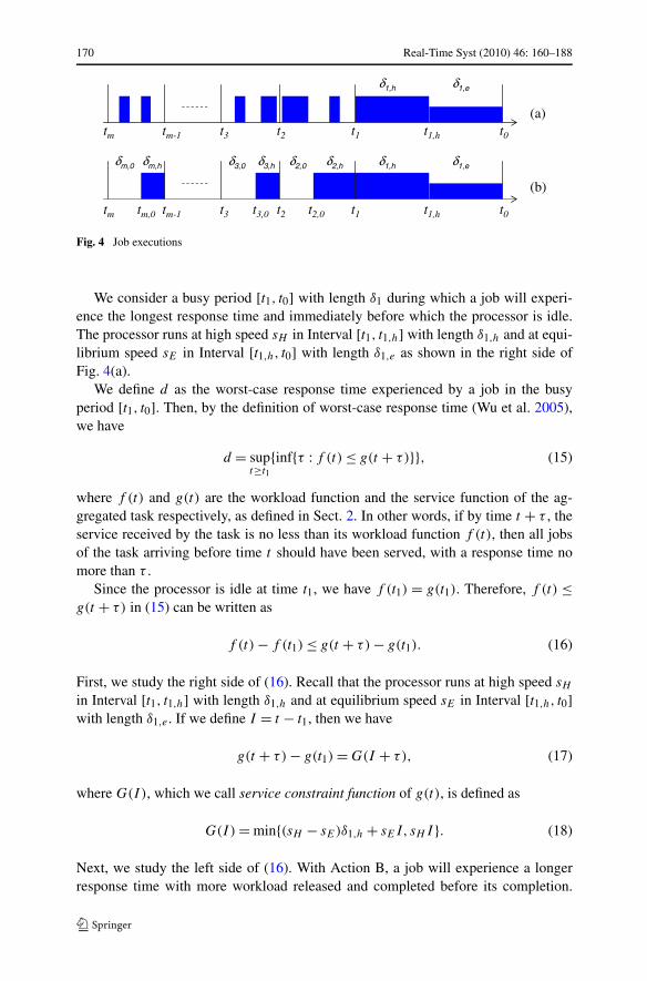
We consider a busy period [t1, t0] with length δ1 during which a job will experi-ence the longest response time and immediately before which the processor is idle.The processor runs at high speed sH in Interval [t1, t1,h] with length δ1,h and at equi-librium speed sE in Interval [t1,h, t0] with length δ1,e as shown in the right side ofFig. 4(a).
We define d as the worst-case response time experienced by a job in the busyperiod [t1, t0]. Then, by the definition of worst-case response time (Wu et al. 2005),we have
d = supt≥t1
{inf{τ : f (t) ≤ g(t + τ)}}, (15)
where f (t) and g(t) are the workload function and the service function of the ag-gregated task respectively, as defined in Sect. 2. In other words, if by time t + τ , theservice received by the task is no less than its workload function f (t), then all jobsof the task arriving before time t should have been served, with a response time nomore than τ .
Since the processor is idle at time t1, we have f (t1) = g(t1). Therefore, f (t) ≤g(t + τ) in (15) can be written as
f (t) − f (t1) ≤ g(t + τ) − g(t1). (16)
First, we study the right side of (16). Recall that the processor runs at high speed sHin Interval [t1, t1,h] with length δ1,h and at equilibrium speed sE in Interval [t1,h, t0]with length δ1,e . If we define I = t − t1, then we have
g(t + τ) − g(t1) = G(I + τ), (17)
where G(I), which we call service constraint function of g(t), is defined as
G(I) = min{(sH − sE)δ1,h + sEI, sH I }. (18)
Next, we study the left side of (16). With Action B, a job will experience a longerresponse time with more workload released and completed before its completion.
Real-Time Syst (2010) 46: 160–188 171
Fig. 5 Response time constraint
Therefore, if we set
f (t) − f (t1) = F(t − t1) = F(I), (19)
then together with (17) the worst-case response time in (16) can be written as
d = supI≥0
{inf{τ : F(I) ≤ G(I + τ)}}. (20)
The above formula is illustrated in Fig. 5.
4.2 Extended busy-period analysis
The above single busy-period is not enough for thermal-constrained schedulabilityanalysis. As we can see, the undetermined service constraint function G(I) is the keyin the worst-case response time formula (20). As defined in (18), G(I) is a functionof δ1,h, which obviously depends on the temperature at time t1. As we mentionedin previous section, the temperature at time t1 will also be affected by earlier jobexecutions. In the following, we will present our extended busy-period schedulabilityanalysis to address this issue.
The exact temperature at t1 is hard to obtain. Instead, we aim to obtain a tightupper-bound of the temperature at t1, which will result in an upper-bound of theworst-case response time according to Lemma 2.
To achieve this, we introduce extra intervals [tk+1, tk]’s (k = 1, . . . ,m − 1), asshown in Fig. 4(a). By Lemma 1, we can use the three actions mentioned earlier toupper-bound the temperature at t1. With Action A, we upper-bound the temperatureat tm by TH . With Action C, for each Interval δk (k = 2, . . . ,m), we shift all partsof job execution to the end of this interval, such that the beginning part is idle withlength δk,0 and the ending part is busy with length δk,h, as shown in Fig. 4(b). Weassume that the temperature will not hit TH during [tm, t1],3 then the processor willrun at high speed sH during each interval [tk+1,0, tk].
In the following, we investigate the service and the thermal interference in theextended busy period.
3If there is an interval [tk0+1, tk0 ] during which the temperature hits TH , then the temperature at tk0 isTH . In this case, we can set m = k0 and remove all intervals on the left.
172 Real-Time Syst (2010) 46: 160–188
4.2.1 Service in extended busy period
We consider the service received in each interval [tk, t0], k = 1, . . . ,m. As shown inFig. 4(b), the executed processor cycles in [tk, t0] can be written as
g(t0) − g(tk) = sH
k∑j=1
δj,h + sEδ1,e. (21)
For k = 1, we have g(t0) − g(t1) = G(t0 − t1) = f (t0) − f (t1). Following theschedulability analysis in the above response time constraint, we consider the worst-case workload f (t0) − f (t1) = F(t0 − t1). Therefore, by (21) we have
sH δ1,h + sEδ1,e = F(δ1,h + δ1,e). (22)
For k = 2, . . . ,m, by the definition of the worst-case response time in (15), wehave f (tk − d) ≤ g(tk). Then together with g(t0) ≤ f (t0) the number of processorcycles in Interval [tk, t0] is bounded as
g(t0) − g(tk) ≤ f (t0) − f (tk − d). (23)
By Lemma 2, the response time will become longer when g(t0)− g(tk) = f (t0)−f (tk − d) = F(t0 − tk + d) by either shifting the job execution or increasing theprocessor cycles of jobs. Therefore, by (21) we have
sH
k∑j=1
δj,h + sEδ1,e = F
(k∑
j=1
δj,h + δ1,e + d
). (24)
Note that the service received by jobs depends on the processing speed, whichchanges with the thermal behavior. Next we want to see how the temperature changesin each interval.
4.2.2 Thermal interference in extended busy period
First, we consider each interval [tk+1, tk], k = 1, . . . ,m− 1, which is composed of anidle period with length δk+1,0 and a busy period with length δk+1,h. Define Tk as thetemperature at tk , then following the temperature formula (7), we have
Tk = asαH
b+
(Tk+1e
−bδk+1,0 − asαH
b
)e−bδk+1,h . (25)
Together with the assumption that Tk ≤ TH and Tm = TH , we have
Tk
TH
=(
sH
sE
)α m∑r=k+1
e−b∑r−1
l=k+1 δl (1 − e−bδr,h ) + e−b∑m
l=k+1 δl ≤ 1. (26)
Next, considering Interval [t1, t1,h], we have
T1
TH
=(
sH
sE
)α
−((
sH
sE
)α
− 1
)ebδ1,h . (27)
Real-Time Syst (2010) 46: 160–188 173
In summary, the above schedulability analysis results in several important concreteconstraint conditions represented by expressions: (20), (22), (24), (26), and (27). Withthese constraint conditions, we are able to obtain a tight upper-bound of the worst-case response time.
Specifically, for any given values of δ1,h, δ1,e , δk,0, and δk,h, k = 2, . . . ,m,which are constrained by (20), (22), (24), (26), and (27), we can obtain anupper-bound of the worst-case response time, which we denote as d(δ1,h, δ1,e ,δ2,0, δ2,h, . . . , δm,0, δm,h). Note that, with any combination of δ1,h, δ1,e , δ2,0, δ2,h, . . . ,
δm,0, and δm,h, d(δ1,h, δ1,e, δ2,0, δ2,h, . . . , δm,0, δm,h) can always bound the worst-case response time. In order to find a tight upper-bound of the worst-case responsetime, we can choose a set of δk,0’s and δk,h’s to minimize d(δ1,h, δ1,e, δ2,0, δ2,h, . . . ,
δm,0, δm,h) as summarized in the following theorem:
Theorem 1 In a system with FIFO scheduling under reactive speed scaling, a tightbound of the worst-case response time d can be obtained by the following formula
d = min{d(δ1,h, δ1,e, δ2,0, δ2,h, . . . , δm,0, δm,h)}subject to (20), (22), (24), (26), and (27). (28)
As we can see, in Theorem 1, if we know the aggregate workload function F(I),then we can obtain d(δ1,h, δ1,e, δ2,0, δ2,h, . . . , δm,0, δm,h). Furthermore, through opti-mization techniques, we can obtain the work-case response time d . As a case study,in the following, we consider a leaky-bucket task workload and have the followingcorollary for the worst-case response time under FIFO scheduling:
Corollary 1 In a system with FIFO scheduling under reactive speed scaling, weconsider tasks whose aggregated-task workload is F(I) = σ + ρI . Define χ1 = sE
sH
and χ2 = ρsH
. A tight bound of the worst-case response time d is expressed as follows:
d ={
V (X − Y), χ2 ≤ χα1
V (X − Y − Z), otherwise(29)
where V = (1−χ1)(1−χ2)χ1−χ2
, X = χ11−χ1
dE , Y = 1b
ln 1−χ21−χα
1, and Z = 1
bχ2
1−χ2ln χ2
χα1
. If we
define dH and dE as the response time when the processor always runs at sH and sErespectively, i.e., dH = σ
sHand dE = σ
sE, then the worst-case response time d is also
constrained by
dH ≤ d ≤ dE. (30)
The proof is given in Appendix A.
5 Schedulability analysis for SP scheduling
Under SP scheduling, jobs from different tasks are assigned different priorities. Low-priority jobs are preempted by high-priority jobs. We assume all jobs from Task Γi
are assigned Priority i. A smaller index indicates a higher priority.
174 Real-Time Syst (2010) 46: 160–188
In order to perform schedulability analysis in the system with SP scheduling, weintroduce the following lemma:
Lemma 3 For any work-conserving scheduling algorithm in a system under reactivespeed scaling as defined in (11), the service function g(t) of the aggregated task isuniquely determined by the workload function f (t) of the aggregated task, not by thescheduling algorithm.
Proof The service function g(t) can be written as
g(t) =∫ t
0s(τ ) dτ, (31)
where s(·) is the processing speed. According to (11), s(t) is determined by W(t) andT (t) under reactive speed scaling, where W(t) is the backlogged workload at time t ,i.e., W(t) = f (t) − g(t), and T (t) is determined by s(t) according to (5). Therefore,the service function g(t) will be uniquely determined by the workload function f (t)
of the aggregated task. We have no assumption of the scheduling algorithm. Hencethe lemma is proved. �
Based on Lemma 3, we are able to obtain the worst-case response time under SPscheduling as shown in the following theorem:
Theorem 2 In a system with SP scheduling under reactive speed scaling, a tightbound of the worst-case response time di for Task Γi can be obtained by the followingformula
di = supI≥0
{inf
{τ :
i−1∑j=1
Fj (I + τ) + Fi(I ) ≤ G(I + τ)
}}, (32)
where G(I) is defined in (18) and δ1,h in G(I) can be obtained by minimizingd(δ1,h, δ1,e, δ2,0, δ2,h, . . . , δm,0, δm,h) in Theorem 1.
Proof We consider a busy interval [t1, t0], during which at least one job from TasksΓj (j ≤ i) is running, and immediately before which no jobs from Tasks Γj (j ≤ i)are running. We know that the response time of a job J of Task Γi is introduced bytwo arrival stages of jobs in the queue: all queued jobs at J ’s release time and thehigher-priority ones coming between J ’s release time and completion time. Then wehave the worst-case response time for a job of Task Γi as follows:
di = supt≥t1
{inf
{τ :
i−1∑j=1
fj (t + τ) + fi(t) ≤i∑
j=1
gj (t + τ)
}}, (33)
where fi(t) and gi(t) are the workload function and the service function of Task Γi ,respectively.
Real-Time Syst (2010) 46: 160–188 175
By our assumption about Interval [t1, t0], we have fj (t1) = gj (t1), j = 1, . . . , i,and gj (t) = gj (t1), j = i + 1, . . . , n. Therefore,
∑i−1j=1 fj (t + τ) + fi(t) ≤∑i
j=1 gj (t + τ) in the above formula can be written as∑i−1
j=1(fj (t + τ) − fj (t1)) +(fi(t) − fi(t1)) ≤ ∑n
j=1(gj (t + τ) − gj (t1)). With the similar analysis for FIFO
scheduling, the worst-case response time happens when∑i−1
j=1(fj (t + τ)−fj (t1))+(fi(t) − fi(t1)) = ∑i−1
j=1 Fj (I + τ) + Fi(I ), where I = t − t1. Then (32) holds. In(32), G(I) is defined in (18). By Lemma 3, the service function under SP schedulingis same as the one under FIFO scheduling. Then δ1,h in G(I) can be obtained byminimizing d(δ1,h, δ1,e, δ2,0, δ2,h, . . . , δm,0, δm,h) in Theorem 1. �
Similarly, in the following we consider the leaky-bucket task workload as a casestudy. We have the following corollary on the worst-case response time for SPscheduling:
Corollary 2 In a system with SP scheduling under reactive speed scaling, we assumethat Task Γi has a workload constraint function Fi(I ) = σi + ρiI . A tight bound ofthe worst-case response time di for Task Γi can be written as
di = max{dE,i − Δ,dH,i}, (34)
where
dE,i =∑i
j=1 σj
sE − ∑i−1j=1 ρj
, (35)
dH,i =∑i
j=1 σj
sH − ∑i−1j=1 ρj
, (36)
Δ =∑n
j=1 σj − sEd
sE − ∑i−1j=1 ρj
, (37)
and d in (37) can be obtained by Corollary 1. dE,i and dE,i are the worst-case re-sponse times under constant speed scaling with speeds sE and sH , respectively.
The proof is given in Appendix B.
6 Schedulability analysis for EDF scheduling
Under EDF scheduling, jobs from a task are assigned priorities on the basis of theirdeadline. The earlier the deadline, the higher the priority. We assume any job in TaskΓi is associated with a deadline Di .
Similar to the schedulability analysis for SP scheduling, we rely on Lemma 3 toobtain the worst-case response time under EDF scheduling as shown in the followingtheorem:
176 Real-Time Syst (2010) 46: 160–188
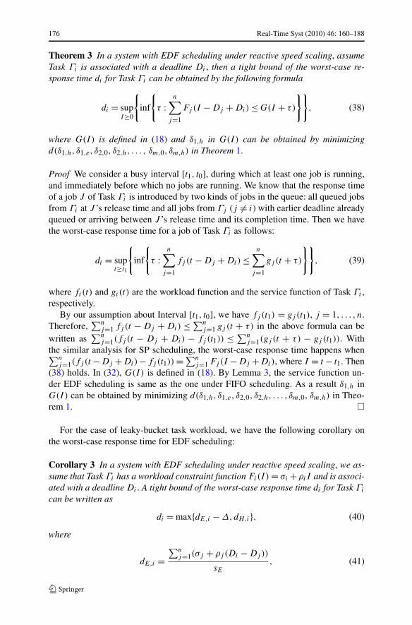
Theorem 3 In a system with EDF scheduling under reactive speed scaling, assumeTask Γi is associated with a deadline Di , then a tight bound of the worst-case re-sponse time di for Task Γi can be obtained by the following formula
di = supI≥0
{inf
{τ :
n∑j=1
Fj (I − Dj + Di) ≤ G(I + τ)
}}, (38)
where G(I) is defined in (18) and δ1,h in G(I) can be obtained by minimizingd(δ1,h, δ1,e, δ2,0, δ2,h, . . . , δm,0, δm,h) in Theorem 1.
Proof We consider a busy interval [t1, t0], during which at least one job is running,and immediately before which no jobs are running. We know that the response timeof a job J of Task Γi is introduced by two kinds of jobs in the queue: all queued jobsfrom Γi at J ’s release time and all jobs from Γj (j �= i) with earlier deadline alreadyqueued or arriving between J ’s release time and its completion time. Then we havethe worst-case response time for a job of Task Γi as follows:
di = supt≥t1
{inf
{τ :
n∑j=1
fj (t − Dj + Di) ≤n∑
j=1
gj (t + τ)
}}, (39)
where fi(t) and gi(t) are the workload function and the service function of Task Γi ,respectively.
By our assumption about Interval [t1, t0], we have fj (t1) = gj (t1), j = 1, . . . , n.Therefore,
∑nj=1 fj (t − Dj + Di) ≤ ∑n
j=1 gj (t + τ) in the above formula can bewritten as
∑nj=1(fj (t − Dj + Di) − fj (t1)) ≤ ∑n
j=1(gj (t + τ) − gj (t1)). Withthe similar analysis for SP scheduling, the worst-case response time happens when∑n
j=1(fj (t −Dj +Di)−fj (t1)) = ∑nj=1 Fj (I −Dj +Di), where I = t − t1. Then
(38) holds. In (32), G(I) is defined in (18). By Lemma 3, the service function un-der EDF scheduling is same as the one under FIFO scheduling. As a result δ1,h inG(I) can be obtained by minimizing d(δ1,h, δ1,e, δ2,0, δ2,h, . . . , δm,0, δm,h) in Theo-rem 1. �
For the case of leaky-bucket task workload, we have the following corollary onthe worst-case response time for EDF scheduling:
Corollary 3 In a system with EDF scheduling under reactive speed scaling, we as-sume that Task Γi has a workload constraint function Fi(I ) = σi +ρiI and is associ-ated with a deadline Di . A tight bound of the worst-case response time di for Task Γi
can be written as
di = max{dE,i − Δ,dH,i}, (40)
where
dE,i =∑n
j=1(σj + ρj (Di − Dj))
sE, (41)
Real-Time Syst (2010) 46: 160–188 177
Fig. 6 Transformation of a non-EDF schedule into an EDF schedule
dH,i =∑n
j=1(σj + ρj (Di − Dj))
sH, (42)
Δ =∑n
j=1 σj
sE− d, (43)
and d in (43) can be obtained by Corollary 1. The expressions for dE,i and dH,i arethe worst-case response time under constant speed scaling with speeds sE and sH ,respectively.
The proof is given in Appendix C.As we know, EDF scheduling is optimal under constant speed scaling (Liu 2000).
Fortunately, we find out that EDF remains optimal under reactive speed scaling asshown in the following theorem:
Theorem 4 EDF scheduling is optimal under reactive speed scaling.
Proof We use the same approach used in the proof of the optimality of EDF underconstant speed scaling (Liu 2000): Any feasible schedule under reactive speed scalingcan be systematically transformed into an EDF schedule.
Suppose that in a schedule, we consider two jobs J1 and J2 as shown in the topfigures in Fig. 6 (a) and (b). We assume each job is scheduled as a whole. Otherwise,we will only consider a successive part of each job. We assume that the deadlines D2of J2 is later than the deadline D1 of J1. If the release time r2 of J2 is later than the
178 Real-Time Syst (2010) 46: 160–188
completion time f1 of J1 (r2 is not shown in the figures), J2 cannot be scheduledbefore f1, and the two jobs are already scheduled on the EDF basis. Therefore, in thefollowing, we assume that r2 is no later than f1.
Without loss of generality, we assume that r2 is no later than the beginning exe-cution time of J1. To transform the given schedule, we swap J1 and J2 as shown inthe figure. Specifically, if the number of processor cycles of J1 is smaller than theone of J2 as shown in Fig. 6(a), we move the portion of J2 that fits in the originalJ1 and move the entire portion of J1 backward to J2 and place it after J2. The swapis always possible because the following fact: By Lemma 3, the service function isuniquely determined by the workload function and not by the scheduling algorithmsuch as FIFO, SP, or EDF. And so are the temperature and speed profiles. If the num-ber of processor cycles of J1 is larger than the one of J2 as shown in Fig. 6(b), wecan do a similar swap. We repeat this transformation for every pair of jobs that arenot scheduled on the EDF basis until no such pair exists.
Since both reactive speed scaling and the considered scheduling algorithms arework-conserving, there will not exist a case that some interval is left idle while thereare jobs ready for execution but scheduled in a later interval.
The above analysis shows that we can always transform a feasible schedule underreactive speed scaling into an EDF schedule. Therefore, EDF scheduling is optimalunder reactive speed scaling. �
7 Performance evaluation
In this section we quantify the benefit of using simple reactive speed scaling by com-paring the worst-case response time with that of a system without speed scaling. Weadopt as the baseline a constant-speed processor that runs at equilibrium speed sE .
We choose the same setting as Skadron et al. (2003) for a silicon chip. The thermalconductivity of the silicon material per unit volume is kth = 100 W/m K and the ther-mal capacitance per unit volume is cth = 1.75e+6 J/m3 K. The chip is tth = 0.55 mmthick. Therefore, the thermal RC time constant RC = cth
ktht2th = 5.3 ms (Skadron et
al. 2003). We choose β0 = 1, β1 = 0.001, and β2 = 0.1. Hence by (4) a = 5.7e−7and b ≈ 188.9 s−1. The ambient temperature is 45◦C and the maximum temperaturethreshold is 85◦C, hence TH = 40◦C. The equilibrium speed sE is fixed by the systemwith (10) and we choose sH = 10
7 sE and assume α = 3.We consider three tasks Γi ’s (i = 1,2,3). Each task Γi has a leaky bucket arrival
with Fi(I ) = σi + ρiI . The aggregate task has an arrival with F(I) = σ + ρI , whereσ = ∑3
i=1 σi and ρ = ∑3i=1 ρi . In our evaluation, we vary σ/sE and ρ/sE in the
ranges of [0,0.005] and [0,0.5] respectively. We compare the worst-case responsetime of jobs in the system under reactive speed scaling and the baseline one in thesystems the processor always run at the equilibrium speed.
First we consider FIFO scheduling. We evaluate the worst-case response time de-crease ratio (dE − d)/dE for the aggregated task.4 Figure 7 shows a contour plot of
4The alert reader has noticed that we did not define a value for parameter a. This is because a appears onlyin the computation of sE , which cancels out in the response time decrease ratio.
Real-Time Syst (2010) 46: 160–188 179
Fig. 7 A contour plot of response time decrease ratio (dE − d)/dE for the aggregated task under reactivespeed scaling for FIFO scheduling
(dE − d)/dE in terms of σ/sE and ρ/sE . Based on (29) and Fig. 7, we observe thatthe response time decrease ratio changes from a minimum 0 (as d = dE) to a maxi-mum of 1 − sE
sH= 0.300 (as d = dH ). The response time decrease ratio will decrease
as either σ or ρ increases.Next we consider SP scheduling. We assume that σ1 : σ2 : σ3 = ρ1 : ρ2 : ρ3 = 1 :
2 : 3. We evaluate the worst-case response time decrease ratio (dE,i − di)/dE,i forTask Γi . Each individual picture in Fig. 8 shows contour plots of (dE,i − di)/dE,i interms of σ/sE and ρ/sE , for the three tasks separately. Based on (34) and Fig. 8, weobserve that the response time decrease ratio changes from a minimum of 0 (as di =dE,i ) to a maximum of 1 − sE
sH= 0.300 for Task Γ1, to a maximum of (1 − sE
sH)/(1 −
16
sEsH
) = 0.316 for Task Γ2, and to a maximum of (1 − sEsH
)/(1 − 12
sEsH
) = 0.353 for
Task Γ3 (as di = dE,i ).As long as the response time decrease ratio is not larger than 0.300, the ratio will
decrease as either σ or ρ increases for any task. Whenever it exceeds 0.300, we havedifferent observation results for the lower-priority tasks. In particular, consideringthe lower-priority task Γ3, once di reaches dH,i , the response time decrease ratio canbe written as (1 − sE
sH)/(1 − 1
sH
∑i−1j=1 ρj ) = 0.300/(1 − 1
sH
∑i−1j=1 ρj ). Therefore, as
shown at the left-bottom corner of the last two contour plots in Fig. 8, the responsetime decrease ratio will keep constant as σ increases and ρ keeps constant, but in-crease beyond 0.300 as ρ increases and σ keeps constant.
Finally, we consider EDF scheduling. We consider the same assumption that σ1 :σ2 : σ3 = ρ1 : ρ2 : ρ3 = 1 : 2 : 3 and the deadlines are D1 = 0.004,D2 = 0.006,D3 =0.008. We evaluate the worst-case response time decrease ratio (dE,i − di)/dE,i forTask Γi . Each individual picture in Fig. 9 shows contour plots of (dE,i − di)/dE,i
in terms of σ/sE and ρ/sE , for the three tasks separately. Based on (40) and Fig. 9,we observe that the response time decrease ratio changes from a minimum of 0 (asdi = dE,i ) to a maximum of 1 − sE
sH= 0.300 for all tasks. And the response time
decrease ratio decreases with the increase of either σ or ρ, except for the case of
180 Real-Time Syst (2010) 46: 160–188
Fig. 8 Contour plots of response time decrease ratio (dE,i − di )/dE,i for Task Γi under reactive speedscaling for SP scheduling
Real-Time Syst (2010) 46: 160–188 181
Fig. 9 Contour plots of response time decrease ratio (dE,i − di )/dE,i for Task Γi under reactive speedscaling for EDF scheduling
182 Real-Time Syst (2010) 46: 160–188
Γ3. In this exception, once d3 < dE,3 (i.e., the response time decrease ratio is below1 − sE
sH= 0.300), by (40), we have (dE,3 − d3)/dE,3 = 1
1+ζ3(dE − d)/dE , where
ζ3 = 1σ
∑3j=1 ρj (D3 − Dj) ≥ 0 and (dE − d)/dE is the response time decrease ratio
for FIFO as shown in Fig. 7. We consider the following two cases:
– Case (dE − d)/dE < 0.300: In this case, ζ3 ≈ 0, then we have (dE,3 − d3)/dE,3 ≈(dE − d)/dE and the curve will be similar to Fig. 7.
– Case (dE − d)/dE = 0.300: In this case, then we have (dE,3 − d3)/dE,3 = 0.3001+ζ3
:as σ increases, ζ3 decreases, then (dE,3 − d3)/dE,3 increases; as ρ increases, ζ3
increases, then (dE,3 − d3)/dE,3 decreases.
8 Conclusion and future work
Schedulability analysis in systems with thermal-constrained speed scaling is difficult,as the traditional definition of “busy period” does not apply, and it becomes difficult toseparate the execution of jobs from the interference by ones arriving earlier or havinglow priorities because of dynamic speed scaling triggered by the thermal behavior. Inthis paper we have shown how to compute bounds on the worst-case response timefor tasks with arbitrary job arrivals for FIFO, SP, and EDF scheduling algorithmsin a system with reactive speed scaling algorithm, which simply runs at maximumspeed until the CPU becomes idle or reaches a critical temperature. In the latter casethe processing speed is reduced (through DVS or appropriate clock throttling) to anequilibrium speed that keeps the temperature constant. We have shown that such ascheme reduces worst-case response time.
In order to further improve the performance of speed scaling, one would have tofind ways to partially isolate jobs from the thermal effects of ones arriving earlier orhaving low priorities. One weakness of the proposed speed-scaling algorithm is itsinability to pro-actively process low-priority tasks at lower-than-equilibrium speeds.
Acknowledgements An earlier version of this work was published in the Proceedings of IEEE Real-Time Systems Symposium, December 2006 (Wang and Bettati 2006). This work was funded by NSF GrantNo. CNS-0509483 and Rackham Faculty Research Grant at the University of Michigan and NSF CAREERGrant No. CNS-0746906.
Appendix A: Proof of Corollary 1
We follow the analysis in Sect. 4 with the leaky bucket workload.
A.1 Single busy-period analysis
Since F(I) = σ + ρI , by (20) we can obtain the response time d as
d = max
{σ
sH,
σ
sE−
(sH
sE− 1
)δ1,h
}. (44)
Real-Time Syst (2010) 46: 160–188 183
Therefore, we have
δ1,h =σsE
− d
sHsE
− 1, (45)
as
d ≥ σ
sH. (46)
A.2 Service in extended busy period
To simplify the service analysis, we consider equal intervals and assume δk = δ
for k = 3, . . . ,m. We investigate the service received in each interval [tk, t0], k =1, . . . ,m.
By (45) and (51), we can rewrite the thermal constraint condition (26).As k = 2, . . . ,m − 1,
Tk
TH
= e−b(m−k)δ(1 − ξ) + ξ, (52)
where
ξ =(
sH
sE
)α 1 − e−b
ρsH
δ
1 − e−bδ. (53)
184 Real-Time Syst (2010) 46: 160–188
By (52), T2 is a function of δ and m. It is easy to show that the smaller T2 is, theshorter the response time d . Therefore, we want to find δ and m to minimize T2 sothat we have a tight upper-bound d of the original worst-case response time.
If ξ ≤ 1, then Tk/TH ≤ 1. By (52), T2 is a decreasing function in terms of (m−2)δ,then T2/TH ≥ lim(m−2)δ→∞ T2/TH = ξ .5 Furthermore, ξ is an increasing functionof δ, then T2/TH ≥ limδ→0 ξ = ( sH
sE)α
ρsH
. Therefore, we choose the minimum andset T2/TH = ( sH
sE)α
ρsH
as ( sHsE
)αρsH
≤ 1.If ξ > 1, then T2/TH is the maximum among all Tk/TH ’s. Therefore, we only
need to consider bound T2/TH ≤ 1. By (52), T2/TH is an increasing function interms of m, then T2/TH will be minimized at m = 2. Hence, we set T2/TH = 1 inthis case.
Therefore, with the analysis above, we can set
T2
TH
= min
{(sH
sE
)αρ
sH,1
}. (54)
At the same time, by (25) and (27), we have
δ1,h + δ2,h = 1
bln
( sHsE
)α − T2TH
e−bδ2,0
( sHsE
)α − 1. (55)
Therefore, by (45), (50), (54), and (55), we can obtain the worst-case responsetime d as follows:
d = (1 − χ1)(1 − χ2)
χ1 − χ2
(χ1
1 − χ1
σ
sE+ χ2
1 − χ2δ2,0 − 1
bln
1 − min{χ2, χα1 }e−bδ2,0
1 − χα1
),
(56)where χ1 = sE
sH, and χ2 = ρ
sH.
Equation (56) shows that d is a function of δ2,0. Since the above analysis worksfor any chosen δ2,0, we want to obtain a minimum d in terms of δ2,0. There are twocases:
– χ2 ≤ χα1 : d will be minimized at δ2,0 = 0, therefore
d = V (X − Y), (57)
– χ2 > χα1 : d will be minimized at δ2,0 = 1
bln χ2
χα1
, therefore
d = V (X − Y − Z), (58)
where V,X,Y,Z are defined in Corollary 1.On the other hand, in the thermal constraint, as k = 1, by (27) and the constraint
that T1/TH ≤ 1, we have
δ1,h ≥ 0. (59)
5We assume that at time zero the system is at lowest temperature. Therefore, we can pick the intervals withoverall length up to infinity.
Real-Time Syst (2010) 46: 160–188 185
Therefore, by (45), we have
d ≤ σ
sE. (60)
Recall that dH = σsH
and dE = σsE
, then by (46) and (60), the worst-case responsetime is also constrained by
dH ≤ d ≤ dE. (61)
Appendix B: Proof of Corollary 2
By Theorem 2, G(I) = min{(sH − sE)δ1,h + sE(I +di), sH (I +di)} depends on δ1,h.For the leaky bucket task workload, by (45) we have δ1,h = ( σ
sE−d)/( sH
sE−1), where
d can be obtained by Corollary 1.By (32), the response time formula can be written as
di = supI≥0
{inf
{τ :
i−1∑j=1
(σj + ρj (I + τ)) + σi + ρiI
≤ min{(sH − sE)δ1,h + sE(I + τ), sH (I + τ)}}}
. (62)
Then, as di > δ1,h, with δ1,h = ( σsE
− d)/( sHsE
− 1), we have
di =∑i−1
j=1(σj + ρjdi) + σi
sE−
(sH
sE− 1
)δ1,h
=∑i−1
j=1(σj + ρjdi) + σi
sE−
(σ
sE− d
)(63)
otherwise
di =∑i−1
j=1(σj + ρjdi) + σi
sH. (64)
Therefore, by (63) and (64), we have
di = max{dE,i − Δ,dH,i}, (65)
where dE,i , dH,i , and Δ are defined in Corollary 2, and d can be obtained by Corol-lary 1. The worst-case response time di is constrained by
dH,i ≤ di ≤ dE,i . (66)
186 Real-Time Syst (2010) 46: 160–188
Appendix C: Proof of Corollary 3
By Theorem 3, G(I) = min{(sH − sE)δ1,h + sE(I +di), sH (I +di)} depends on δ1,h.For the leaky bucket task workload, by (45) we have δ1,h = ( σ
sE−d)/( sH
sE−1), where
d can be obtained by Corollary 1.By (38), the response time formula can be written as
di = supI≥0
{inf
{τ :
n∑j=1
(σj + ρj (I − Dj + Di))
≤ min{(sH − sE)δ1,h + sE(I + τ), sH (I + τ)}}}
. (67)
Then, as di > δ1,h, with δ1,h = ( σsE
− d)/( sHsE
− 1), we have
di =∑n
j=1(σj + ρj (Di − Dj))
sE−
(sH
sE− 1
)δ1,h
=∑n
j=1 ρj (Di − Dj)
sE+ d, (68)
otherwise
di =∑n
j=1(σj + ρj (Di − Dj))
sH. (69)
Therefore, by (68) and (69), we have
di = max{dE,i − Δ,dH,i}, (70)
where dE,i , dH,i , and Δ are defined in Corollary 3, and d can be obtained by Corol-lary 1. The worst-case response time di is constrained by
dH,i ≤ di ≤ dE,i . (71)
References
Advanced configuration and power interface specification (2010) http://www.acpi.info/spec.htm. The lastaccess time is July 2010
Semiconductor Industry Association (2005) 2005 international technology roadmap for semiconductors.http://public.itrs.net. The last access time is July 2010
Bansal N, Kimbrel T, Pruhs K (2005) Dynamic speed scaling to manage energy and temperature. In: IEEEsymposium on foundations of computer science
Bansal N, Pruhs K (2005) Speed scaling to manage temperature. In: Symposium on theoretical aspects ofcomputer science
Brooks D, Martonosi M (2001) Dynamic thermal management for high-performance microprocessors. In:The 7th international symposium on high-performance computer architecture, pp 171–182
Chantem T, Dick RP, Hu XS (2008) Temperature-aware scheduling and assignment for hard real-timeapplications on MPSoCs. In: Design, automation and test in Europe
Chen J-J, Hung C-M, Kuo T-W (2007) On the minimization of the instantaneous temperature for periodicreal-time tasks. In: IEEE real-time and embedded technology and applications symposium
Cohen A, Finkelstein L, Mendelson A, Ronen R, Rudoy D (2003) On estimating optimal performance ofCPU dynamic thermal management. In: Computer architecture letters
Cohen A, Finkelstein L, Mendelson A, Ronen R, Rudoy D (2006) On estimating optimal performance ofCPU dynamic thermal management. In: Computer architecture letters
Dhodapkar A, Lim CH, Cai G, Daasch WR (2000) TEMPEST: a thermal enabled multi-model power/performance estimator. In: Workshop on power-aware computer systems, ASPLOS-IX
Ferreira AP, Oh J, Moss D (2006) Toward thermal-aware load-distribution for real-time server. In: IEEEreal-time systems symposium work-in-progress session
Gochman S, Mendelson A, Naveh A, Rotem E (2006) Introduction to Intel Core Duo processor architec-ture. Intel Technol J 10(2):89–97
Liu J (2000) Real-time systems. Prentice Hall, New YorkRabaey JM, Chandrakasan A, Nikolic B (2002) Digital integrated circuits, 2nd edn. Prentice Hall, New
YorkRao R, Vrudhula S, Chakrabarti C, Chang N (2006) An optimal analytical solution for processor speed
control with thermal constraints. In: International symposium on low power electronics and design.ACM Press, New York
Rotem E, Naveh A, Moffie M, Mendelson A (2004) Analysis of thermal monitor features of the IntelPentium M processor. In: Workshop on temperature-aware computer systems
Sanchez H, Kuttanna B, Olson T, Alexander M, Gerosa G, Philip R, Alvarez J (1997) Thermal managementsystem for high performance powerpc microprocessors. In: IEEE international computer conference
Skadron K, Stan M, Huang W, Velusamy S, Sankaranarayanan K, Tarjan D (2003) Temperature-aware mi-croarchitecture: extended discussion and results. Technical report CS-2003-08, Department of Com-puter Science, University of Virginia
Srinivasan J, Adve SV (2003) Predictive dynamic thermal management for multimedia applications. In:International conference on supercomputing
Tiwari V, Singh D, Rajgopal S, Mehta G, Patel R, Baez F (1998) Reducing power in high-performancemicroprocessors. In: Design automation conference, pp 732–737
Wang S, Bettati R (2006) Delay analysis in temperature-constrained hard real-time systems with generaltask arrivals. In: IEEE real-time systems symposium
Wang S, Bettati R (2008) Reactive speed control in temperature-constrained real-time systems. Real-TimeSyst J 39(1–3), 658–671
Wu J, Liu J, Zhao W (2005) On schedulability bounds of static priority schedulers. In: IEEE real-time andembedded technology and applications symposium
Xu R, Zhu D, Rusu C, Melhem R, Moss D (2005) Energy efficient policies for embedded clusters. In:ACM SIGPLAN/SIGBED conference on languages, compilers, and tools for embedded systems
Zhang S, Chatha KS (2007) Approximation algorithm for the temperature-aware scheduling problem. In:IEEE/ACM international conference on computer-aided design
Shengquan Wang received his B.S. degree in Mathematics from An-hui Normal University, China, in 1995, and his M.S. degree in AppliedMathematics from the Shanghai Jiao Tong University, China. He alsoreceived M.S. degree in Mathematics in 2000 and Ph.D. in ComputerScience from Texas A& M University. He is currently Assistant Profes-sor in the Department of Computer and Information Science at the Uni-versity of Michigan-Dearborn. He is a recipient of the US National Sci-ence Foundation (NSF) Faculty Early Career Development (CAREER)Award. His research interests are in real-time systems, networking anddistributed systems, and security and privacy.
188 Real-Time Syst (2010) 46: 160–188
Youngwoo Ahn received his B.S. degree in electrical engineeringfrom Seoul National University, Korea, in 1997 and his M.S. degreefrom Seoul National University, Korea, in 1999. During 1999–2004,he worked as a research engineer at LG Electronics in Korea. Also heworked at electronics and Telecommunication Research Institute in Ko-rea from 2004 to 2005 as a researcher. He graduated with the Ph.D. inelectrical and computer engineering from Texas A& M University inAugust 2010. His research interests lie primarily in real-time operatingsystems, especially in designing and analyzing task scheduling underresource constraints.
Riccardo Bettati received the diploma in informatics from the SwissFederal Institute of Technology (ETH), Zurich, Switzerland, in 1988and the PhD degree from the University of Illinois, Urbana-Champaign,in 1994. He is currently a professor in the Department of Computer Sci-ence and Engineering, Texas A& M University. His research interestsare in traffic analysis and privacy, realtime distributed systems, real-time communication, and network support for resilient distributed ap-plications. From 1993 to 1995, he held a postdoctoral position at theInternational Computer Science Institute, Berkeley, and at the Univer-sity of California, Berkeley. He is a member of the IEEE ComputerSociety.