140
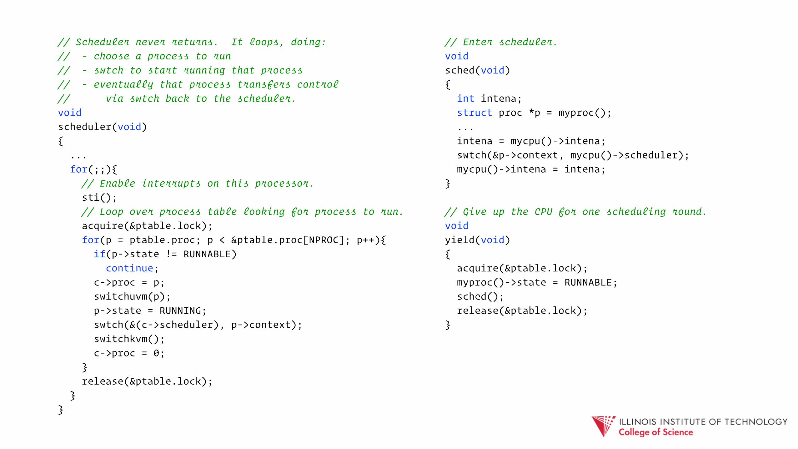
// Scheduler never returns. It loops, doing: // - choose a process to run // - swtch to start running that process // - eventually that process transfers control // via swtch back to the scheduler. void scheduler(void) { ... for(;;){ // Enable interrupts on this processor. sti(); // Loop over process table looking for process to run. acquire(&ptable.lock); for(p = ptable.proc; p < &ptable.proc[NPROC]; p++){ if(p->state != RUNNABLE) continue; c->proc = p; switchuvm(p); p->state = RUNNING; swtch(&(c->scheduler), p->context); switchkvm(); c->proc = 0; } release(&ptable.lock); } }
// Enter scheduler. void sched(void) { int intena; struct proc *p = myproc(); ... intena = mycpu()->intena; swtch(&p->context, mycpu()->scheduler); mycpu()->intena = intena; }
// Give up the CPU for one scheduling round. void yield(void) { acquire(&ptable.lock); myproc()->state = RUNNABLE; sched(); release(&ptable.lock); }

§ Overview

scheduling: policies & mechanisms used to allocate resources to some set of entities
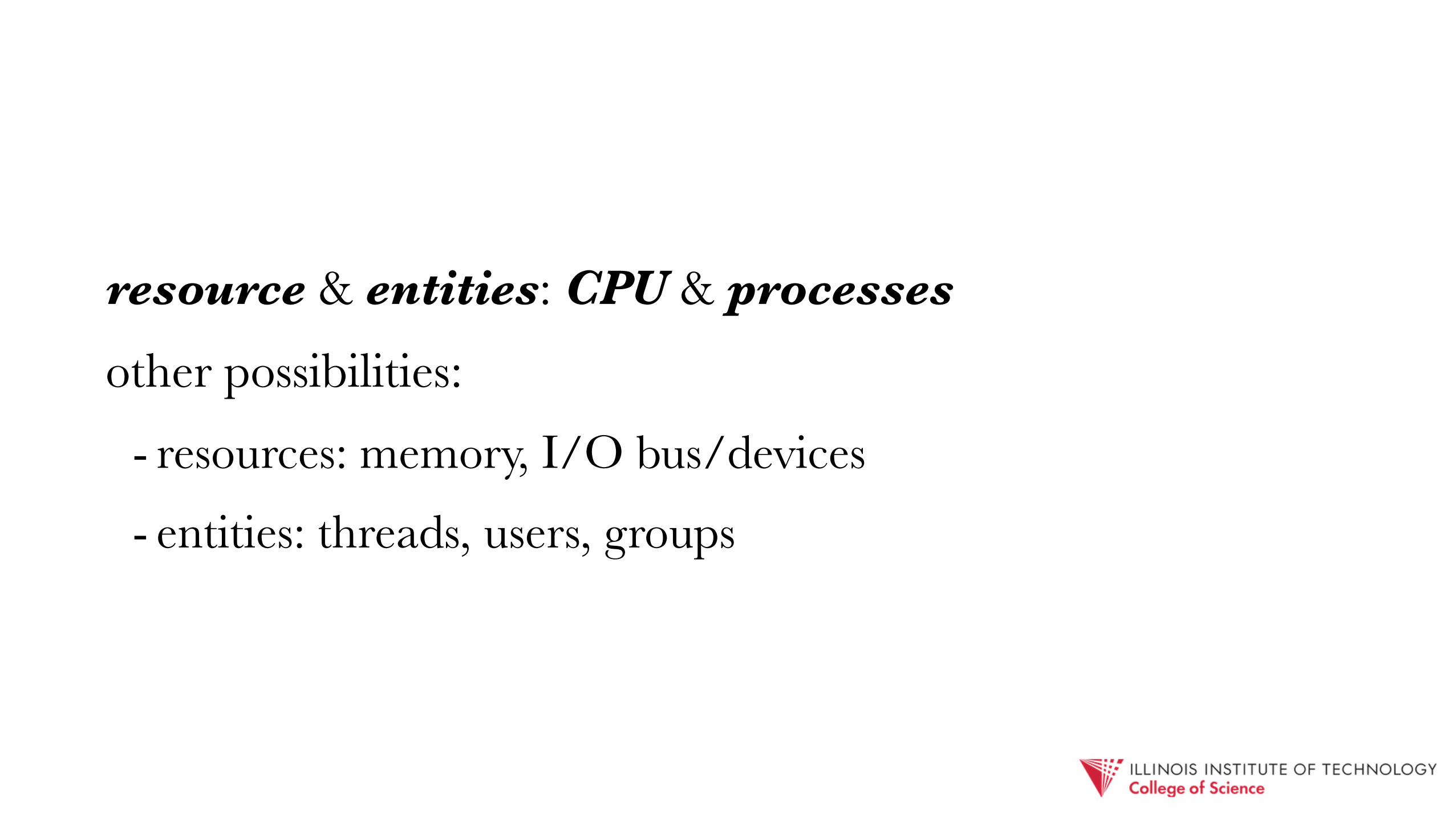
resource & entities: CPU & processes
other possibilities: - resources: memory, I/O bus/devices
- entities: threads, users, groups
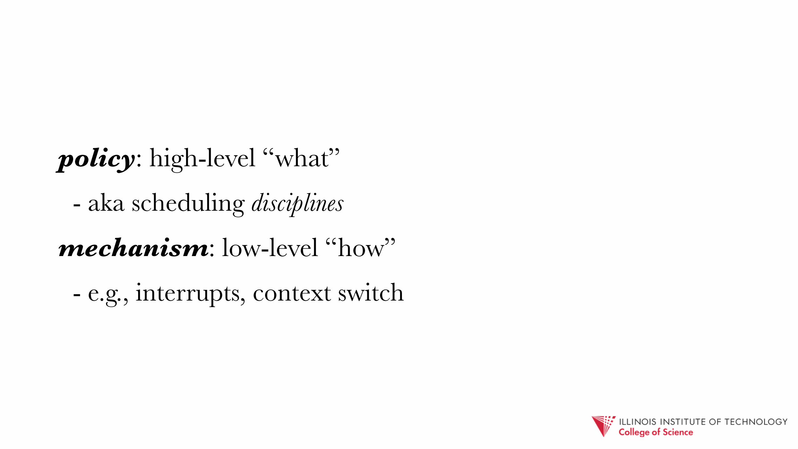
policy: high-level “what” - aka scheduling disciplines
mechanism: low-level “how” - e.g., interrupts, context switch
(we’ll start with policy first)
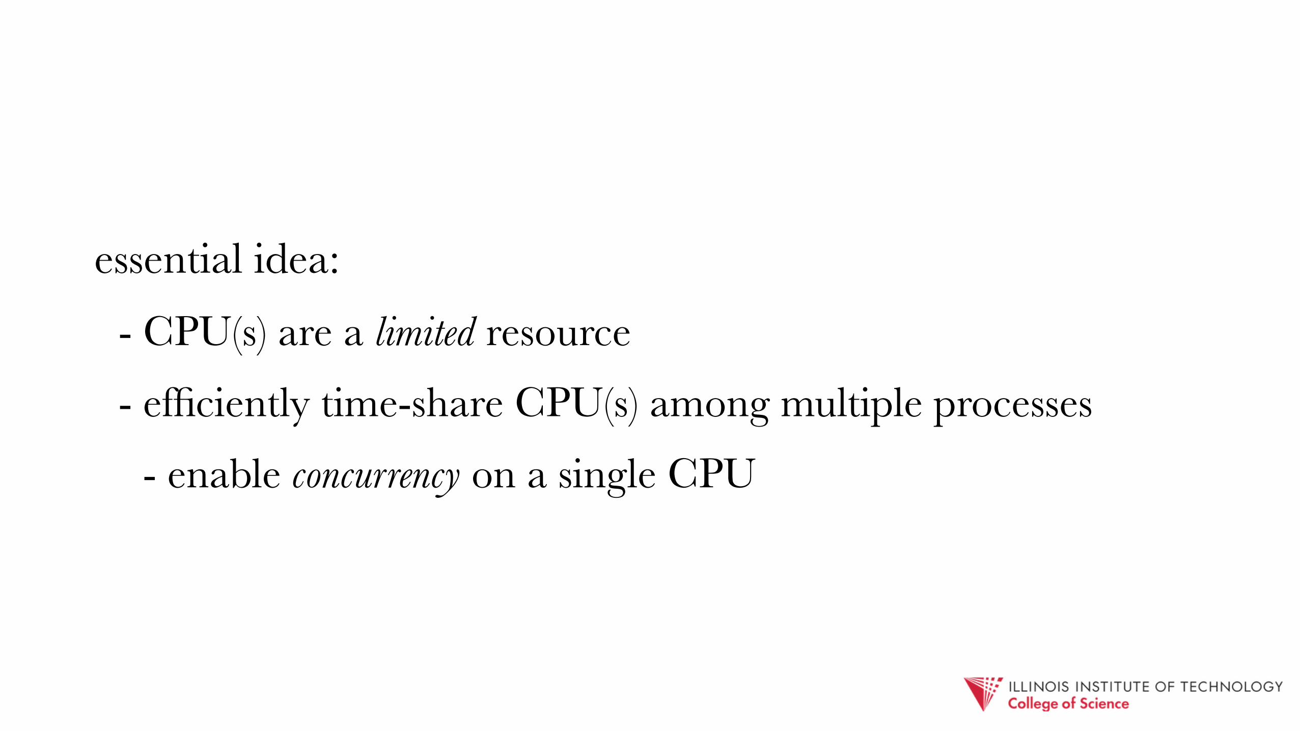
essential idea: - CPU(s) are a limited resource
- efficiently time-share CPU(s) among multiple processes
- enable concurrency on a single CPU

at a high level (policy), only concern ourselves with macro process state one of running, ready, or blocked

running = consuming CPU
ready = “runnable”, but not running
blocked = not runnable (e.g., waiting for I/O)

Ready
Running
Blocked
I/O request(e.g., interrupt, syscall)scheduled
I/O completion
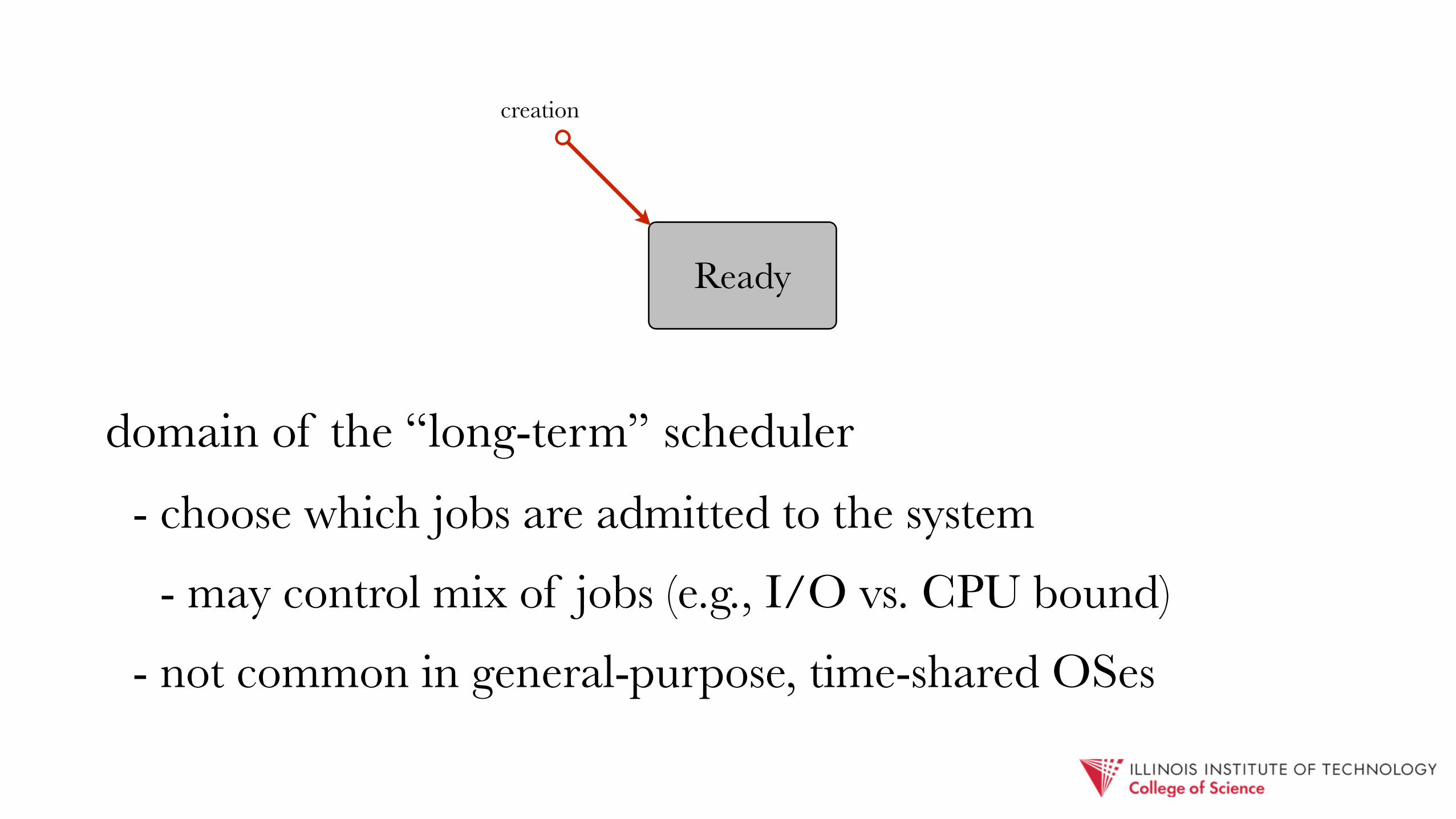
creation
completion
Ready Blocked
swap in/out swap in/out
preempted
Ready
creation
domain of the “long-term” scheduler - choose which jobs are admitted to the system
- may control mix of jobs (e.g., I/O vs. CPU bound)
- not common in general-purpose, time-shared OSes

domain of the “medium-term” scheduler - swaps processes out to disk to make room for others
- active when there is insufficient memory
- runs much less frequently (slower!) than CPU scheduler
Ready Blocked
swap in/out swap in/out

Ready
Runningscheduled
preempted
CPU scheduler, aka “short-term” scheduler - chooses between in-memory, ready processes to run on CPU
- invoked to carry out scheduling policies after interrupts/traps

preemptive scheduling
☑ running → ready transition
- relies on clock interrupt (to regain control of CPU)

non-preemptive scheduling
☒ running → ready transition
- NB: non-preemptive ≠ batch!

Ready
Runningscheduled
convenient to envision a ready queue/set the scheduling policy decides which process to run next from the queue of active, ready processes
policies vary by: 1. preemptive vs. non-preemptive
2. factors used in selecting a process
3. goals; i.e., why are we selecting a given process?

scheduling goals are usually predicated on optimizing certain scheduling metrics — can be provable or based on heuristics
§ Scheduling Metrics

metrics we’ll be concerned with: - turnaround time
- wait time
- response time
- throughput
- utilization
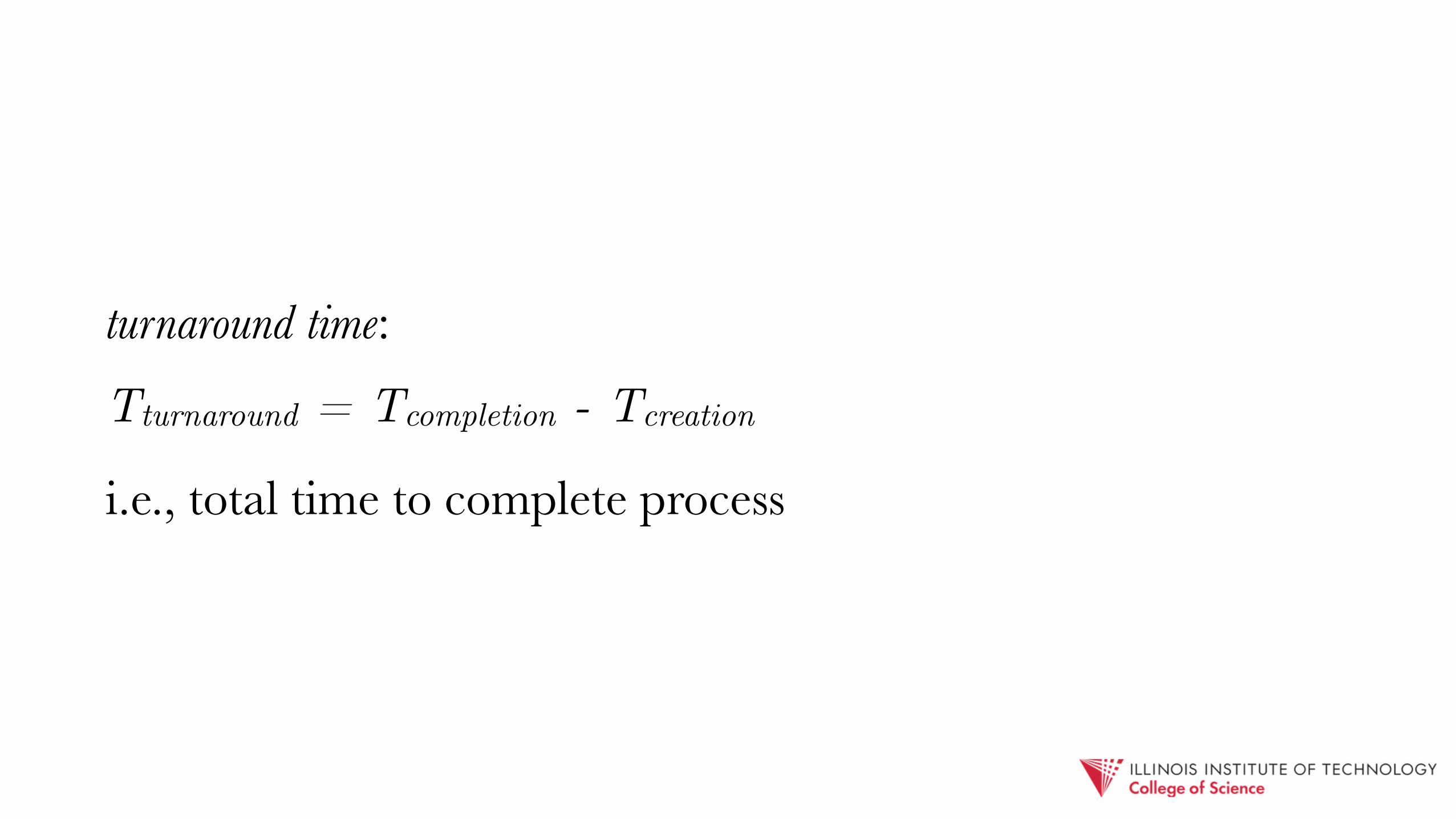
turnaround time:
Tturnaround = Tcompletion - Tcreation
i.e., total time to complete process

turnaround time depends on much more than the scheduling discipline!
- process / program complexity
- I/O processing time
- how many CPUs available - how many other processes need to run

wait time: time spent in ready queue
i.e., how long does the scheduler force a runnable process to wait for a CPU
- better gauge of scheduler’s effectiveness

turnaround & wait time are measured over the course of an entire process — sometimes refer to as the “job”
- not a very useful metric for interactive processes
- which typically alternate between CPU & I/O bursts, indefinitely

5.4 Silberschatz, Galvin and Gagne ©2005Operating System Concepts – 7th Edition, Feb 2, 2005
Alternating Sequence of CPU And I/O BurstsAlternating Sequence of CPU And I/O Bursts
“bursty” execution

5.5 Silberschatz, Galvin and Gagne ©2005Operating System Concepts – 7th Edition, Feb 2, 2005
Histogram of CPUHistogram of CPU--burst Timesburst Times
burst length histogram
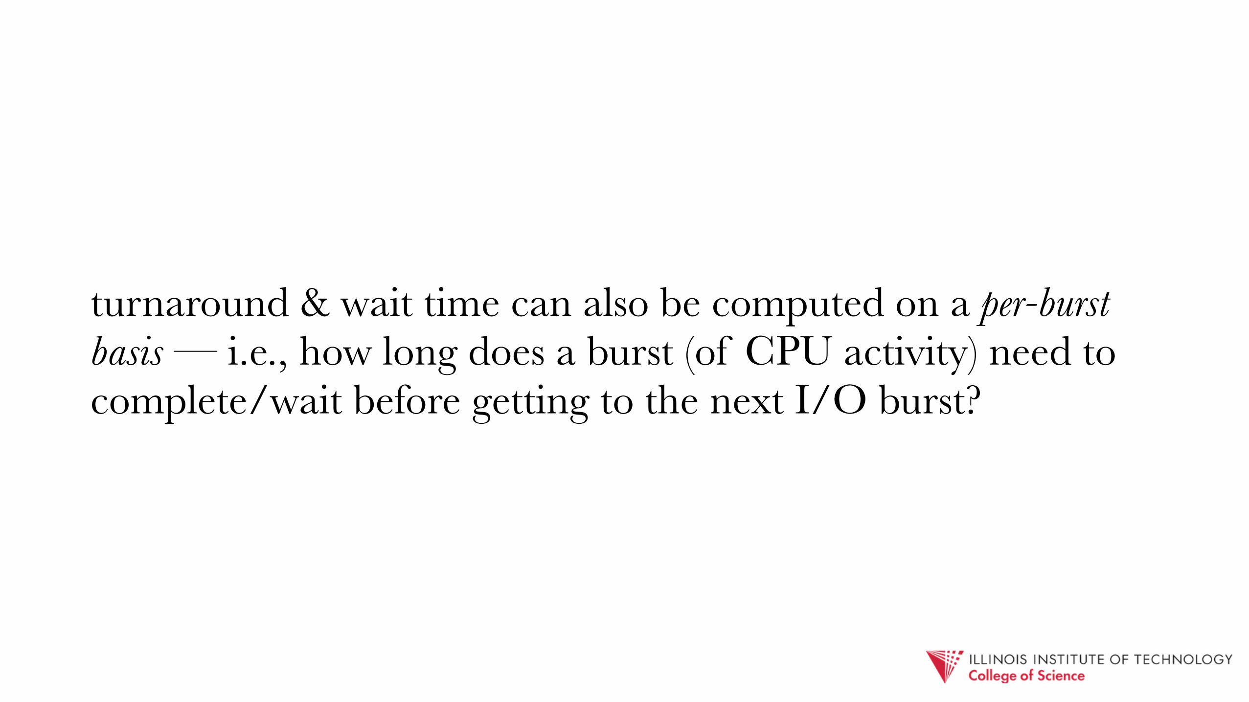
turnaround & wait time can also be computed on a per-burst basis — i.e., how long does a burst (of CPU activity) need to complete/wait before getting to the next I/O burst?

For interactive jobs, improving responsiveness is arguably more important than optimizing total turnaround/wait times
- how to quantify responsiveness (in a way that is useful for scheduling)?

response time: Tresponse = Tfirstrun - Tarrival
- i.e., how soon is a job given a chance to run after arriving?
- NB: still no guarantee that job itself will be responsive (what does this depend on?)

throughput: number of completed jobs or bursts per time unit (e.g., N/sec)
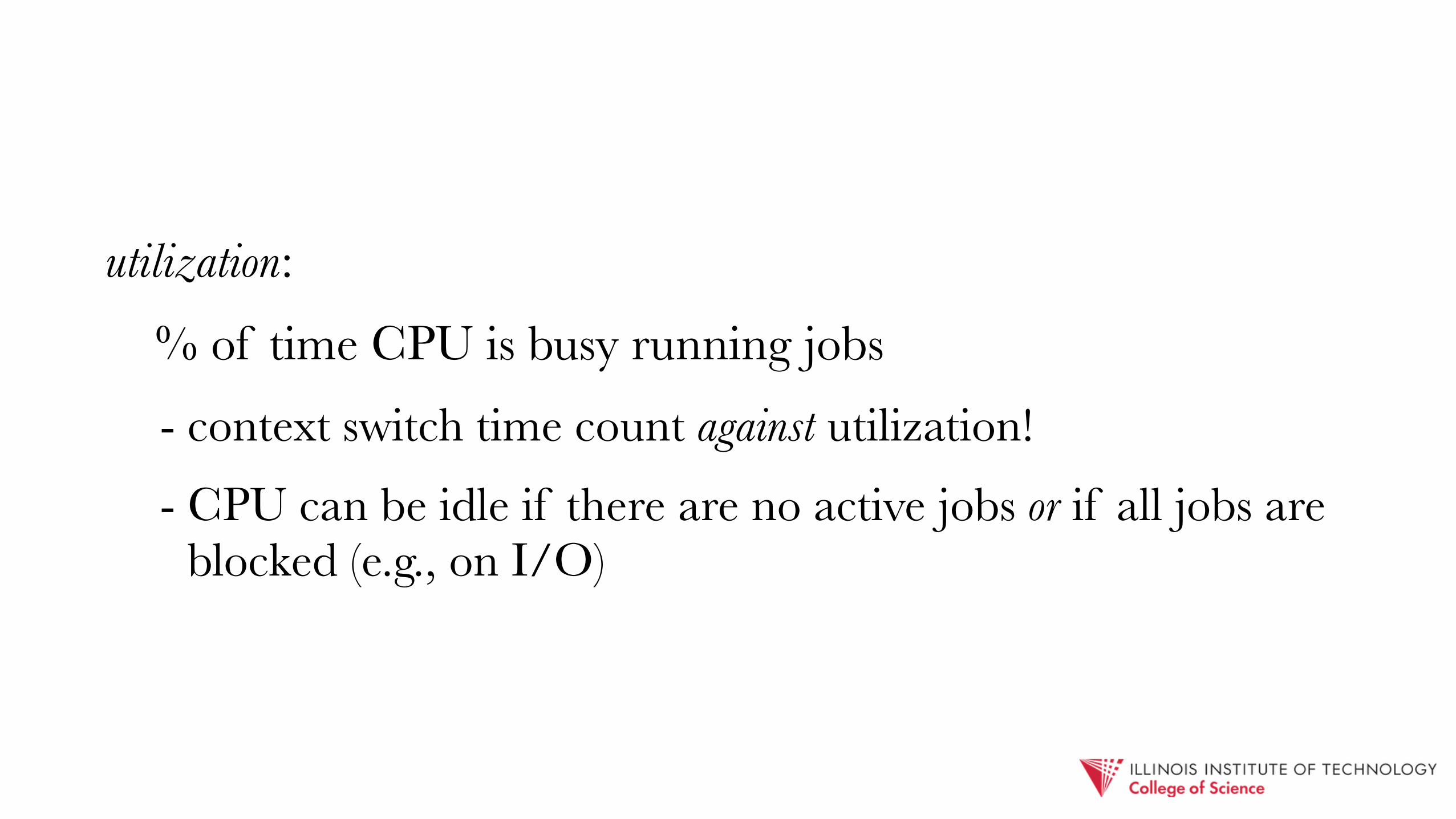
utilization:
% of time CPU is busy running jobs - context switch time count against utilization!
- CPU can be idle if there are no active jobs or if all jobs are blocked (e.g., on I/O)

another (subjective) metric: fairness - what does this mean?
- how to measure it?
- is it useful?
- how to enforce it?

Review (scheduling metrics): - turnaround time (total & per-burst)
- wait time (total & per-burst) - response time - throughput - utilization

§ Scheduling Policies

1. First Come First Served (FCFS)

Process Arrival Time Burst TimeP1 0 24P2 0 3P3 0 3
Wait times: P1 = 0, P2 = 24, P3 = 27 Average: (0+24+27)/3 = 17
P1 P2 P3
24 27 300 “Gantt chart”

Convoy Effect

Process Arrival Time Burst TimeP3 0 3P2 0 3P1 0 24
P3 P2 P1
3 6 300
Wait times: P1 = 6, P2 = 3, P3 = 0 Average: (6+3+0)/3 = 3

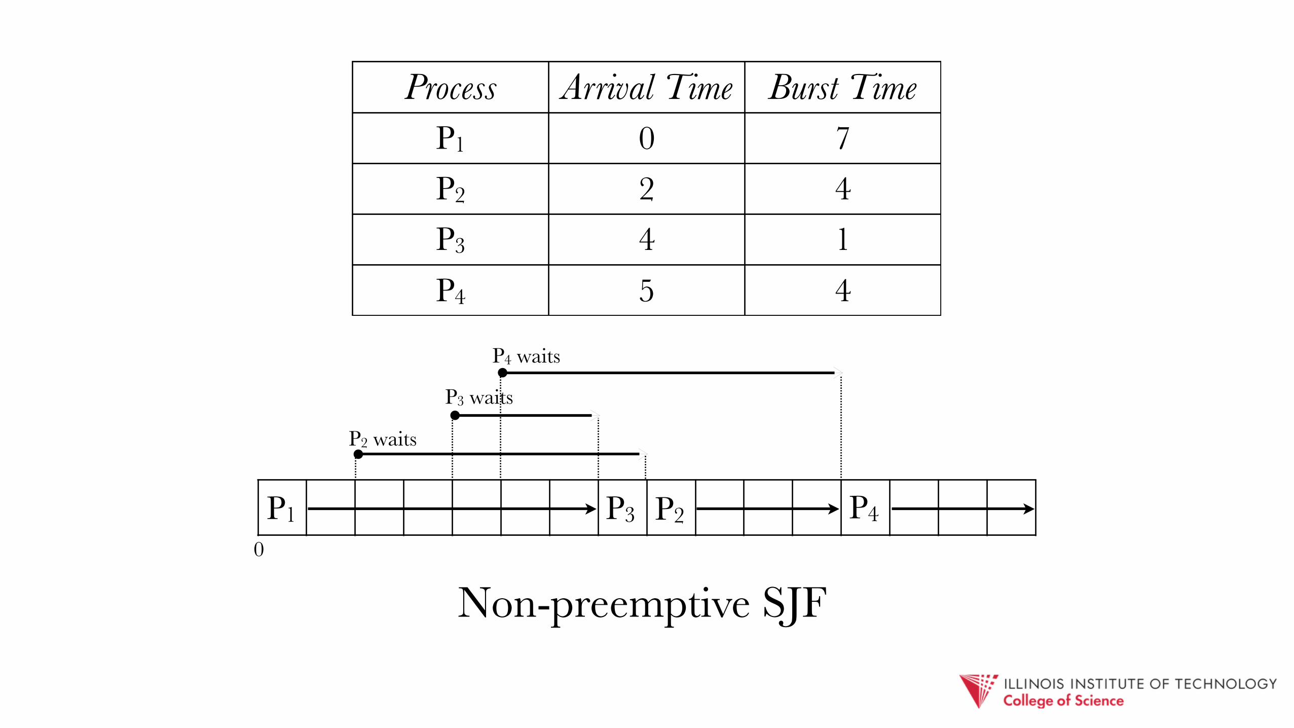
2. Shortest Job First (SJF)
0
Process Arrival Time Burst TimeP1 0 7P2 2 4P3 4 1P4 5 4
P2 waits
P3 waits
P4 waits
P1 P3 P2 P4
Non-preemptive SJF

Wait times: P1 = 0, P2 = 6, P3 = 3, P4=7 Average:(0+6+3+7)/4 = 4
P2 waits
P3 waits
P4 waits
P1 P3 P2 P40
Process Arrival Time Burst TimeP1 0 7P2 2 4P3 4 1P4 5 4

can we do better?
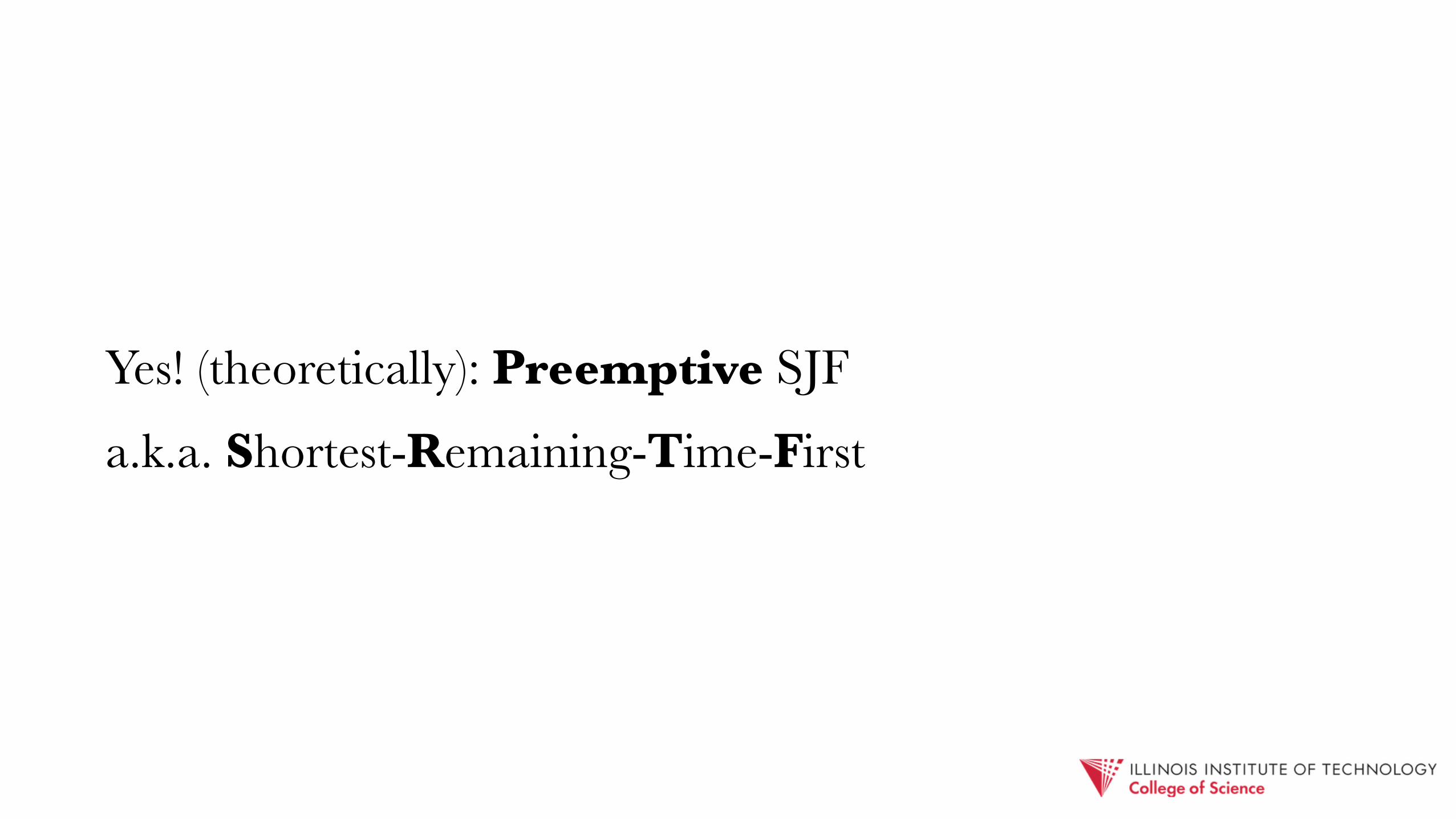
Yes! (theoretically): Preemptive SJF
a.k.a. Shortest-Remaining-Time-First

P1 P3 P40
P2 P2 P1
P1 waits
P2 waits
P4 waits
Process Arrival Time Burst TimeP1 0 7P2 2 4P3 4 1P4 5 4

P1 P3 P40
P2 P2 P1
P1 waits
P2 waits
P4 waits
Wait times: P1 = 9, P2 = 1, P3 = 0, P4 = 2 Average: (9+1+0+2)/4 = 3
Process Arrival Time Burst TimeP1 0 7P2 2 4P3 4 1P4 5 4

SJF/SRTF are greedy algorithms;
i.e., they always select the local optima greedy algorithms don’t always produce globally optimal results (e.g., hill-climbing)
- is preemptive-SJF optimal?

consider 4 jobs arriving at t=0, with burst lengths t0, t1, t2, t3
avg. wait time if scheduled in order?
=3t0 + 2t1 + t2
4

— a weighted average; clearly minimized by running shortest jobs first.
I.e., SJF/PSJF are provably optimal w.r.t. wait time!
=3t0 + 2t1 + t2
4
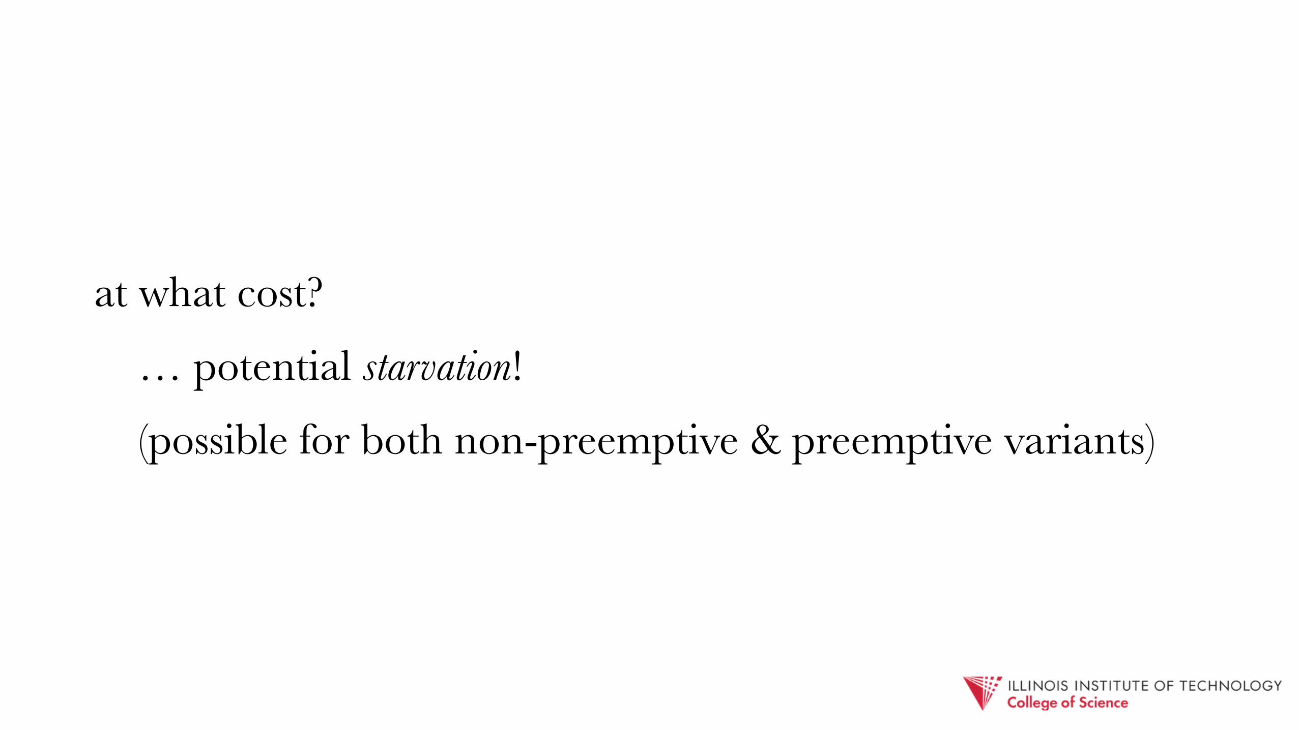
at what cost?
… potential starvation!
(possible for both non-preemptive & preemptive variants)

also, we’ve been making two simplifying assumptions: 1. burst lengths are known in advance
2. context switch time = 0

typically predict future burst lengths based on past behavior - simple moving average (using a sliding window of past values)
- exponentially weighted moving average (EMA)

Observed: ρn-1
Estimated: σn-1
Weight (α): 0 ≤ α ≤ 1
EMA: σn = α⋅ρn-1 + (1–α)⋅σn-1
i.e., bigger α = more credence given to measured burst lengths

Actual Avg (3) Error EMA Error
4 5.00 1.00 5.00 1.00 EMA Alpha: 0.25 4.00 1.00 4.80 0.205 4.50 0.50 4.84 0.166 4.67 1.33 4.87 1.13
13 5.33 7.67 5.10 7.9012 8.00 4.00 6.68 5.3211 10.33 0.67 7.74 3.266 12.00 6.00 8.39 2.397 9.67 2.67 7.92 0.925 8.00 3.00 7.73 2.73
Avg err: 2.78 2.50
0.0
2.6
5.2
7.8
10.4
13.0
Actual Avg (3) EMA
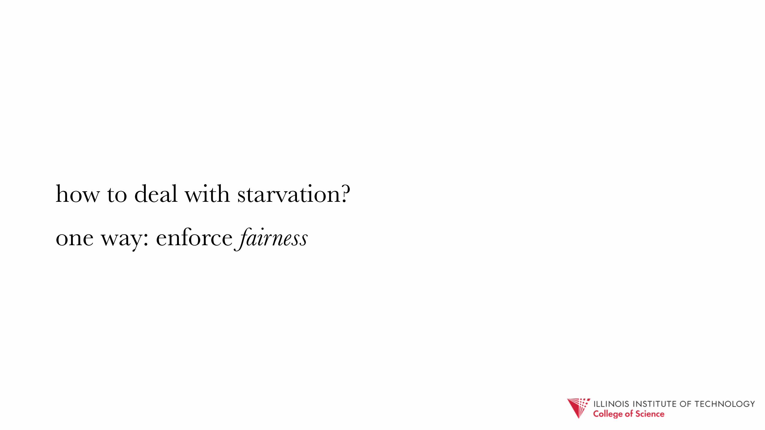
how to deal with starvation?
one way: enforce fairness

3. Round Robin (RR): the “fairest” of them all - FIFO queue
- each job runs for max time quantum q - if unfinished, re-enter queue at back

Given time quantum q and n jobs: - max wait time = q ∙ (n – 1)
- each job receives 1/n timeshare

P1 waitsP2 waits
P1 waitsP2 waits
P3 waits
P4 waits P4 waits
P1 P30
P2 P1 P4 P2 P1 P4
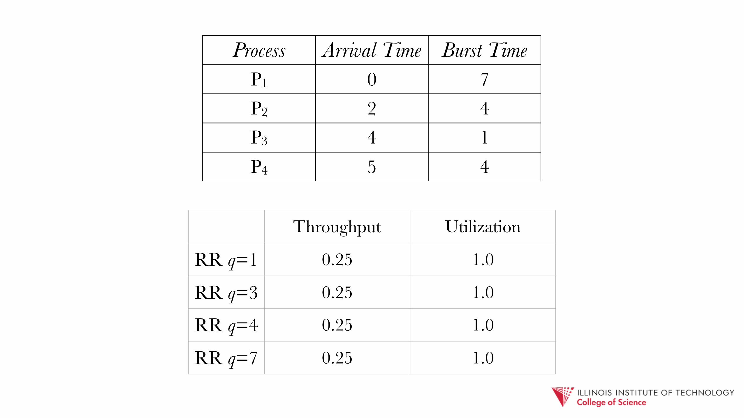
Process Arrival Time Burst TimeP1 0 7P2 2 4P3 4 1P4 5 4
Round Robin, q=3

P1 waitsP2 waits
P1 waitsP2 waits
P3 waits
P4 waits P4 waits
P1 P30
P2 P1 P4 P2 P1 P4
Process Arrival Time Burst TimeP1 0 7P2 2 4P3 4 1P4 5 4
Wait times: P1 = 8, P2 = 8, P3 = 5, P4 = 7 Average: (8+8+5+7)/4 = 7

Process Arrival Time Burst TimeP1 0 7P2 2 4P3 4 1P4 5 4
Avg. Turnaround Avg. Wait Time
RR q=1 9.75 5.75
RR q=3 11 7
RR q=4 9 5
RR q=7 8.75 4.75
Process Arrival Time Burst TimeP1 0 7P2 2 4P3 4 1P4 5 4
Throughput Utilization
RR q=1 0.25 1.0
RR q=3 0.25 1.0
RR q=4 0.25 1.0
RR q=7 0.25 1.0

What happens when we add in context switch times?

Process Arrival Time Burst TimeP1 0 7P2 2 4P3 4 1P4 5 4
Avg. Turnaround Avg. Wait Time
RR q=1 20.25 13.25
RR q=3 16.25 11.25
RR q=4 11.5 7.25
RR q=7 10.25 6.25
(CST=1)

Process Arrival Time Burst TimeP1 0 7P2 2 4P3 4 1P4 5 4
Throughput Utilization
RR q=1 0.125 0.5
RR q=3 0.167 0.667
RR q=4 0.19 0.762
RR q=7 0.2 0.8
(CST=1)

CST = fixed, systemic overhead - increasing quantum relative to CST amortizes the cost
- shorter q = worse utilization; longer q ⟶ FIFO
- NB: cost of context switches is not just the constant CST!
- Also: cache flush/reload, VM swapping, etc.

generally, try to choose q to help tune responsiveness (i.e., of interactive jobs)
may use: - predetermined burst-length threshold (for interactive jobs)
- median of EMAs
- process profiling

RR prevents starvation, and allows both CPU-hungry and interactive jobs to share resources fairly
- but at the cost of utilization and turnaround times!

Can exercise more fine-grained control by introducing a system of arbitrary priorities
- computed and assigned to jobs dynamically by scheduler
- highest (current) priority goes next

SJF is an example of a priority scheduler! - jobs are weighted using a burst-length prediction algorithm
(e.g., EMA)
- priorities may vary over job lifetimes

Recall: SJF is prone to starvation
Common issue for priority schedulers - combat with aging

4. Highest Penalty Ratio Next (HPRN) - a priority scheduler that uses aging to avoid starvation
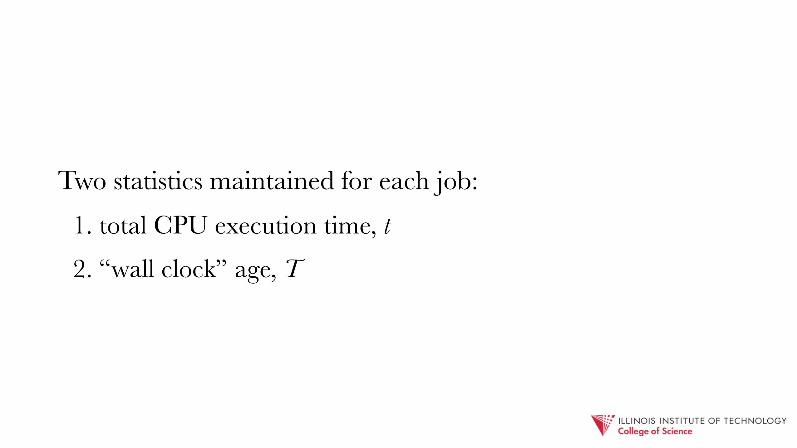
Two statistics maintained for each job: 1. total CPU execution time, t 2. “wall clock” age, T
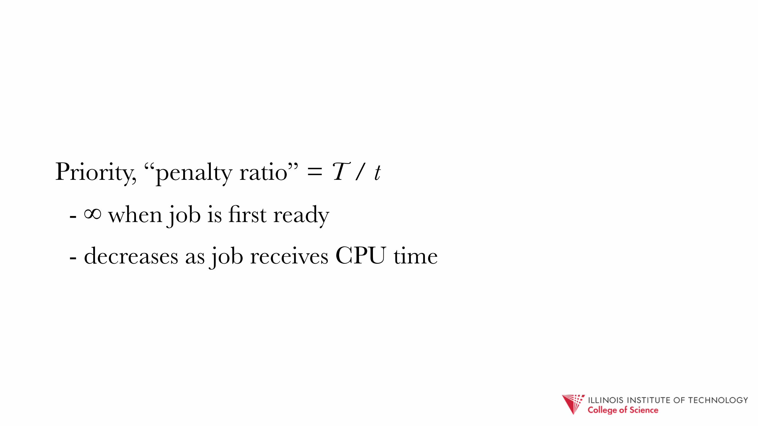
Priority, “penalty ratio” = T / t - ∞ when job is first ready
- decreases as job receives CPU time
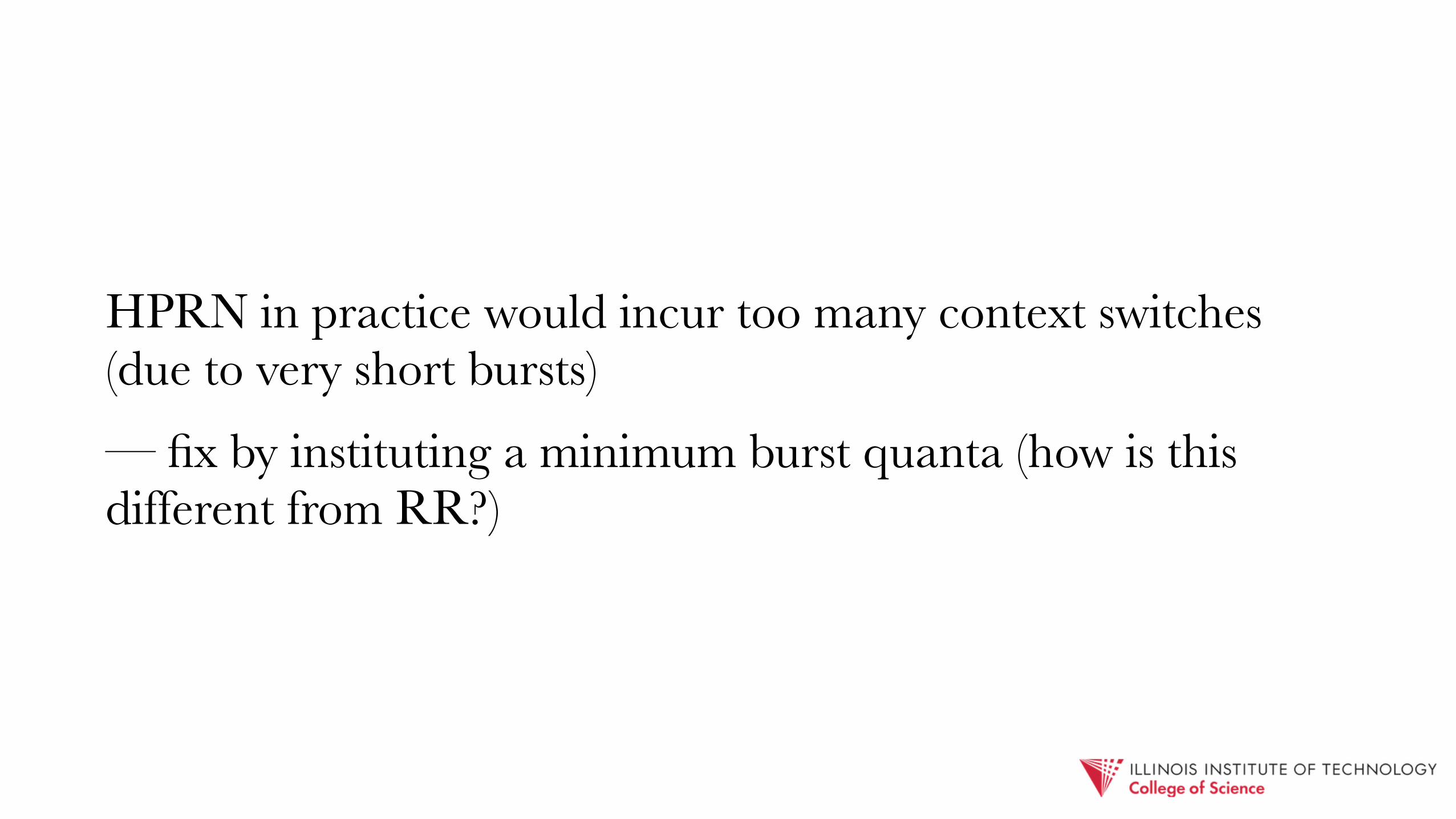
HPRN in practice would incur too many context switches (due to very short bursts)
— fix by instituting a minimum burst quanta (how is this different from RR?)

5. Selfish RR - a more sophisticated priority based scheduling policy

priority ↑ α
priority ↑ β
β = 0 : RR
β ≥ (α ≠ 0) : FCFS
β > (α = 0) : RR in batches
α > β > 0 : “Selfish” (ageist) RR
active (RR)CPU
holdingarriving

Another problem (on top of starvation) possibly created by priority-based scheduling policies: priority inversion

Process Priority StateP1 High ReadyP2 Mid ReadyP3 Mid ReadyP4 Low Ready
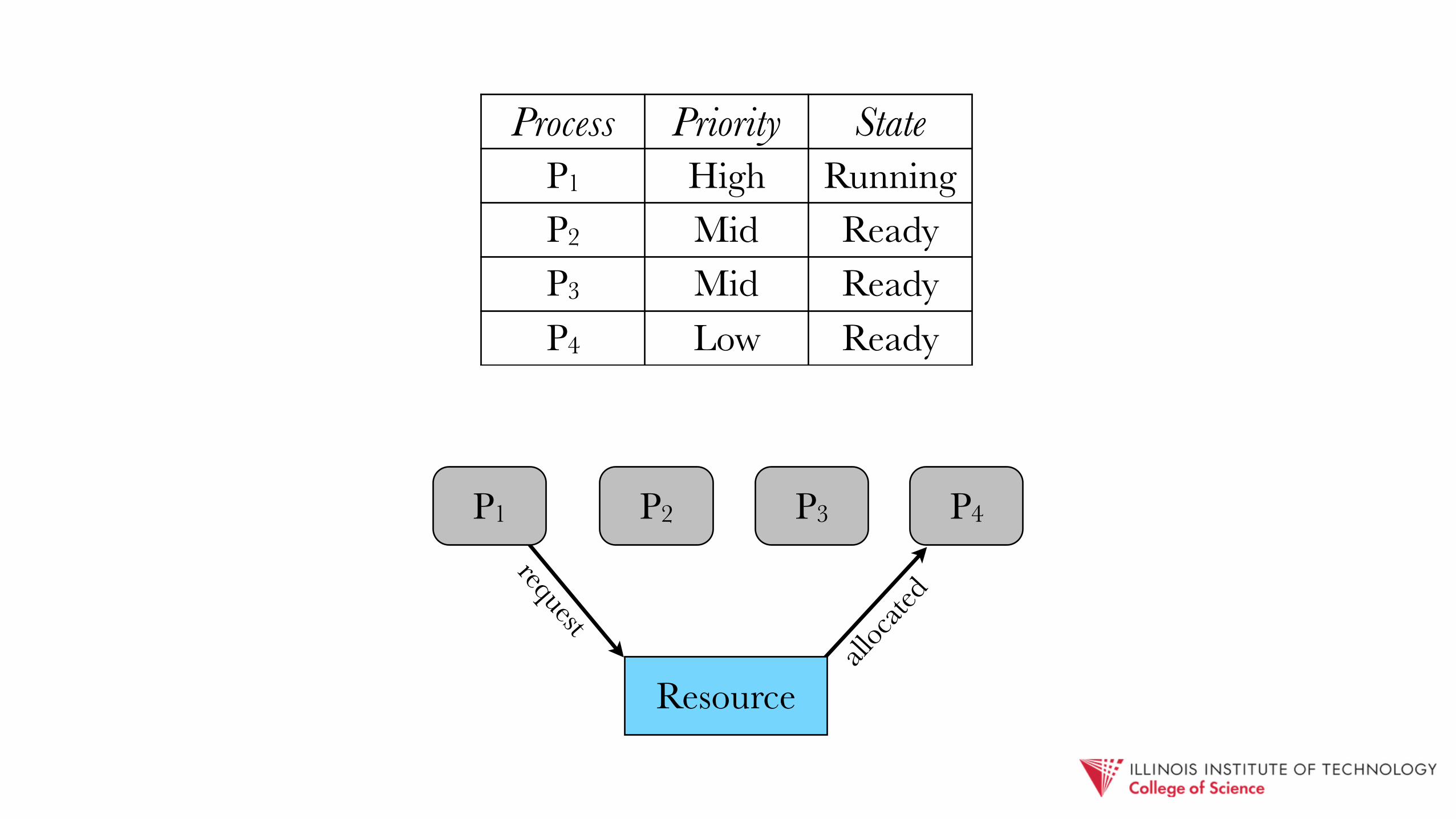
requestall
ocate
d
Process Priority StateP1 High RunningP2 Mid ReadyP3 Mid ReadyP4 Low Ready
Resource
P1 P2 P4P3

Process Priority StateP1 High BlockedP2 Mid ReadyP3 Mid ReadyP4 Low Ready
request
P1 P2 P4
Resource
P3
alloc
ated
(mutually exclusive allocation)

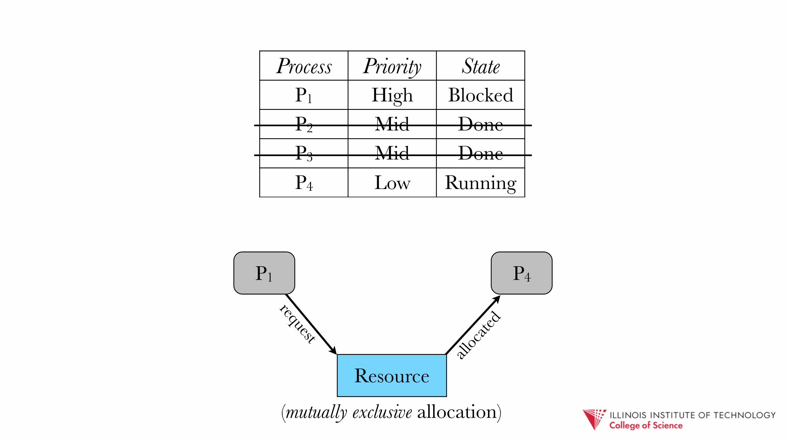
Process Priority StateP1 High BlockedP2 Mid RunningP3 Mid ReadyP4 Low Ready
request
P1 P2 P4
Resource
P3
alloc
ated
(mutually exclusive allocation)

request
P1 P4
Resource
P3
alloc
ated
Process Priority StateP1 High BlockedP2 Mid DoneP3 Mid RunningP4 Low Ready
(mutually exclusive allocation)
request
P1 P4
Resource
alloc
ated
Process Priority StateP1 High BlockedP2 Mid DoneP3 Mid DoneP4 Low Running
(mutually exclusive allocation)

request
P1
Resource
Process Priority StateP1 High BlockedP2 Mid DoneP3 Mid DoneP4 Low Done
(mutually exclusive allocation)
P1
Resource
allocated
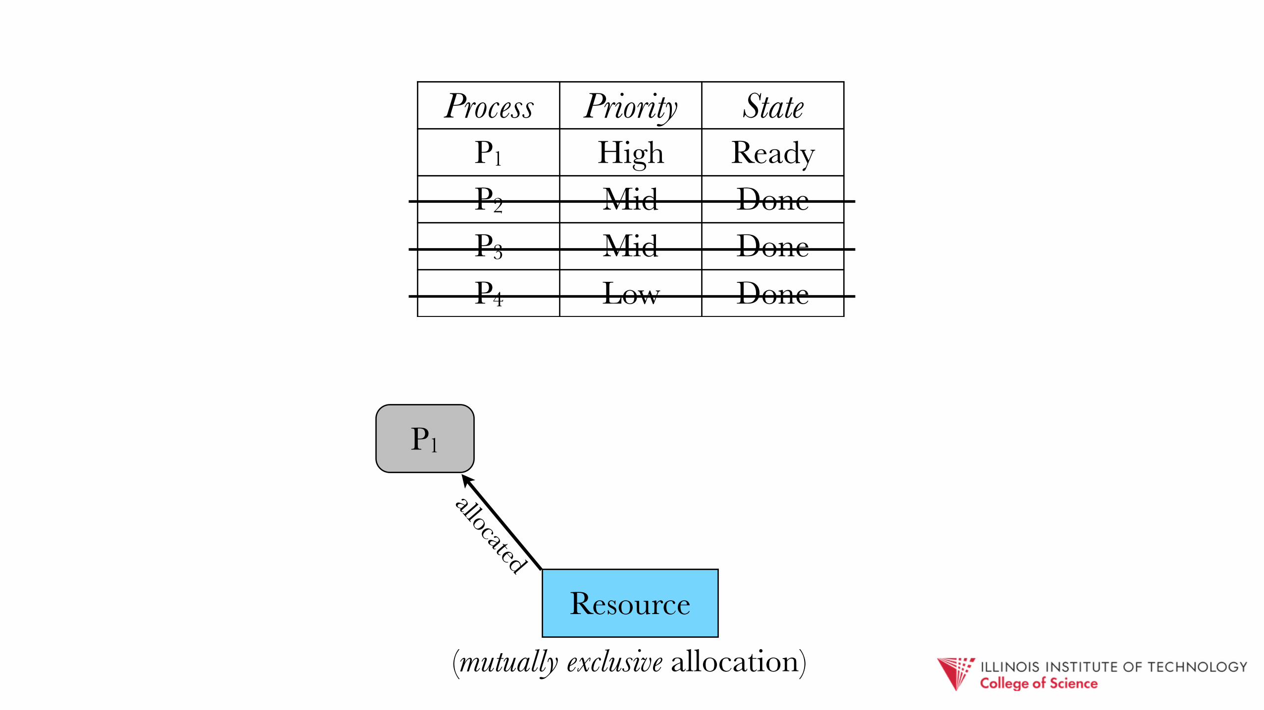
Process Priority StateP1 High ReadyP2 Mid DoneP3 Mid DoneP4 Low Done
(mutually exclusive allocation)
P1
Resource
allocated
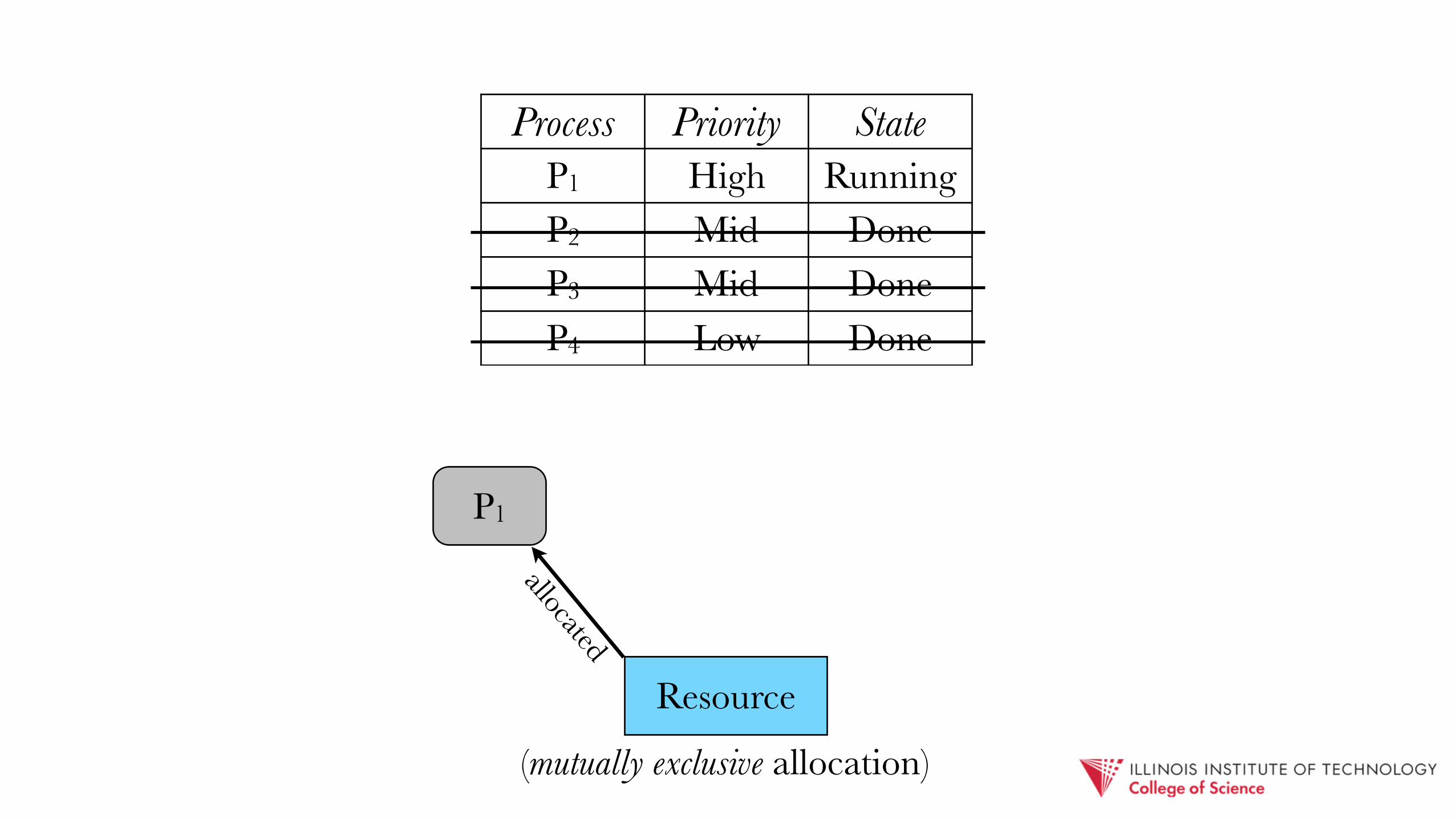
Process Priority StateP1 High RunningP2 Mid DoneP3 Mid DoneP4 Low Done
(mutually exclusive allocation)

priority inversion: a high priority job effectively takes on the priority of a lower-level one that holds a required resource

high profile case study: NASA Pathfinder - spacecraft developed a recurring system failure/reset
- occurred after deploying robot to surface of Mars

culprits: - flood of meteorological data
- low priority of related job: ASI/MET
- a shared, mutually exclusive resource (semaphore guarding an IPC pipe)

high priority job (for data aggregation & distribution) — bc_dist — required pipe
- but always held by ASI/MET
- in turn kept from running by various mid-priority jobs

scheduling job determined that bc_dist couldn’t complete per hard deadline
- declared error resulting in system reset!
- re-produced in lab after 18-hours of on-Earth simulation

fix: priority inheritance - job blocking a higher priority job will inherit the latter’s priority
- e.g., run ASI/MET at bc_dist’s priority until resource released

how? - enabling priority inheritance via semaphores (in vxWorks)
- (why wasn’t it on by default?)
- prescient remote tracing/patching facilities built in to system

why did NASA not foresee this?
“Our before launch testing was limited to the “best case” high data rates and science activities… We did not expect nor test the “better than we could have ever imagined” case.”
- Glenn Reeves Software team lead
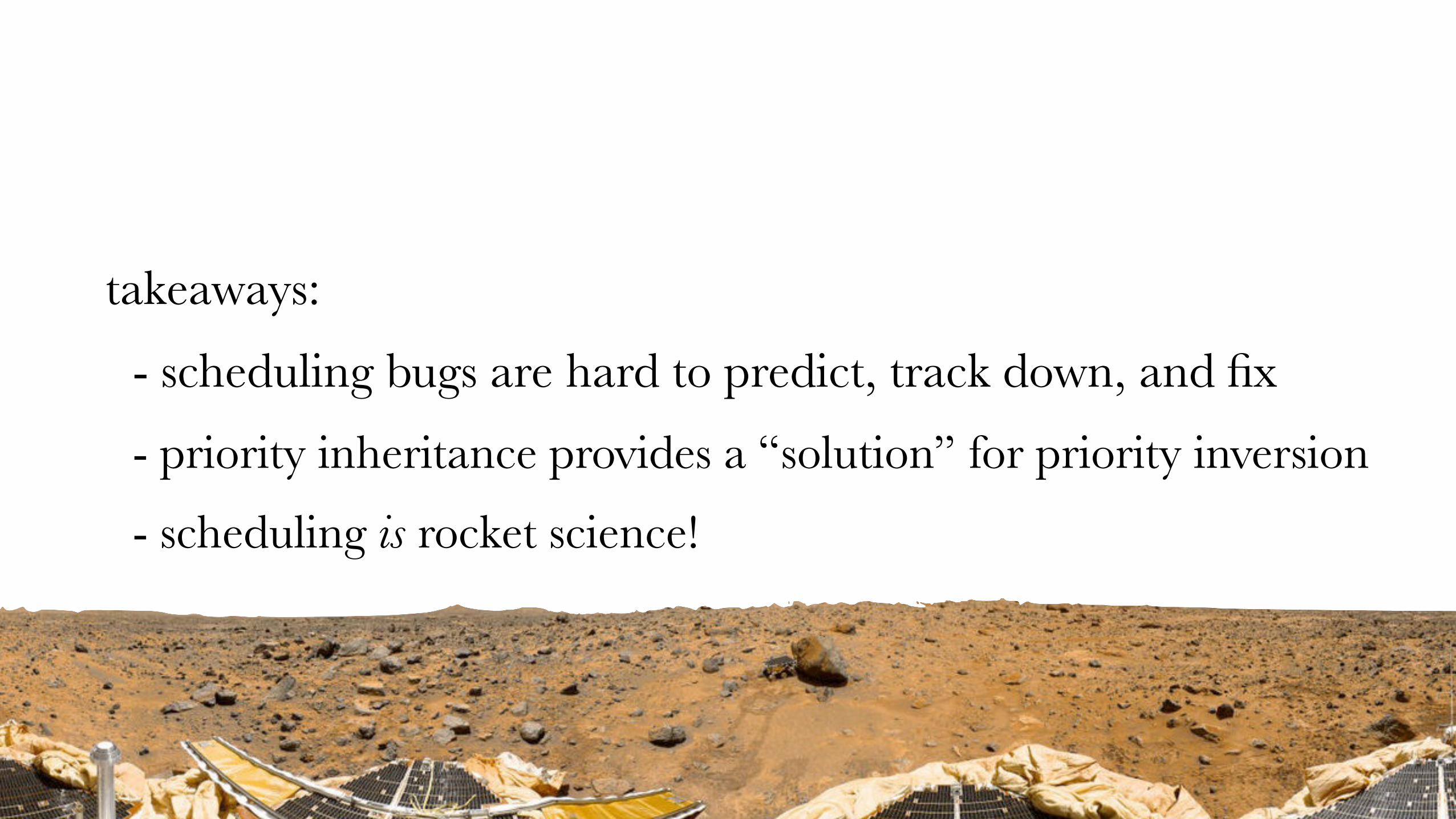
takeaways:
- scheduling bugs are hard to predict, track down, and fix - priority inheritance provides a “solution” for priority inversion
- scheduling is rocket science!
questions: - w.r.t. priority inheritance:
- pros/cons?
- how to implement?
- w.r.t. priority inversion:
- detection? how else to “fix”?
- effect on non-real-time OS?

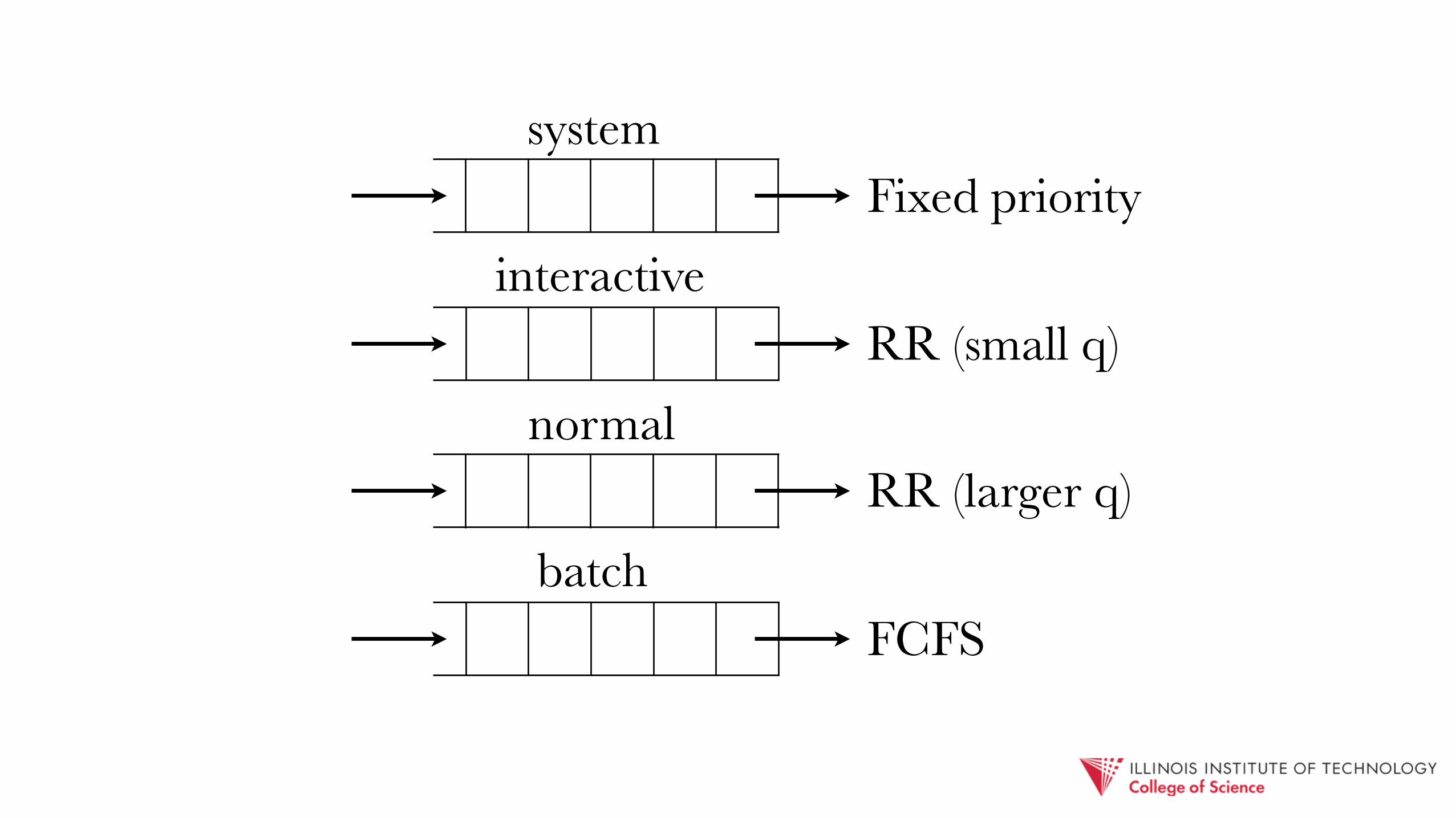
Even with fine-grained control offered by a priority scheduler, hard to impose different sets of goals on groups of jobs
E.g., top-priority for system jobs, RR for interactive jobs, FCFS for batch jobs

6. Multi-Level Queue (MLQ) - disjoint ready queues
- separate schedulers/policies for each
Fixed priority
RR (small q)
FCFS
RR (larger q)
system
interactive
batch
normal

requires queue arbitration strategy in place

Fixed priority
RR (small q)
FCFS
RR (larger q)
system
interactive
batch
normal
decr
easin
g pr
iorit
y
approach 1: prioritize top, non-empty queue

Fixed priority
RR (small q)
FCFS
RR (larger q)
system
interactive
batch
normal
approach 2: aggregate time slices
30%
15%
50%
5%

what processes go in which queues? - self-assigned
- e.g., UNIX “nice” value
- “profiling” based on initial burst(s)
- CPU, I/O burst length
- e.g., short, intermittent CPU bursts ⇒ classify as interactive job

classification issue: what if job requirements change dynamically? - e.g., photo editor: tool selection (interactive) ➞ apply filter
(CPU hungry) ➞ simple edits (interactive)

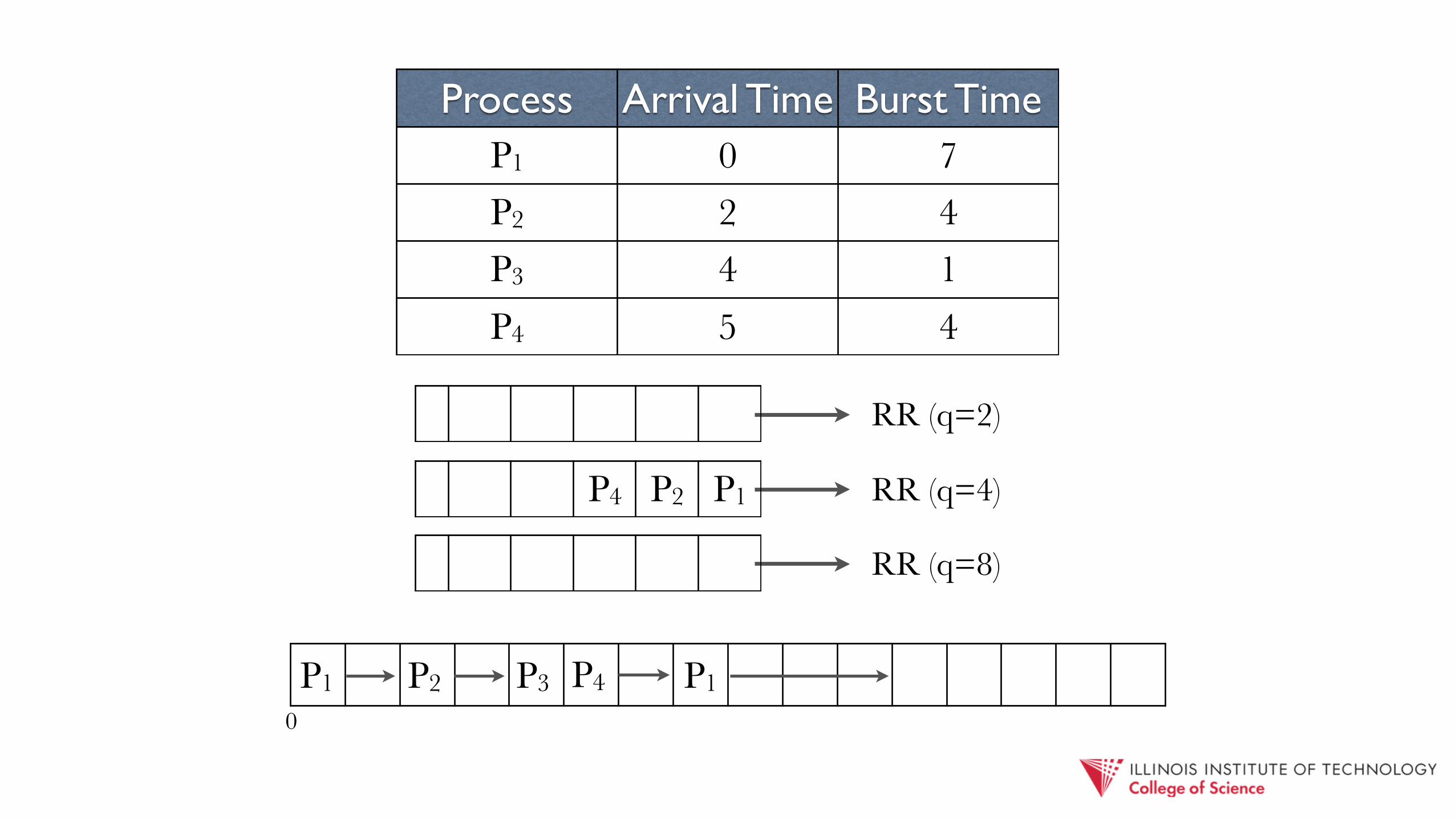
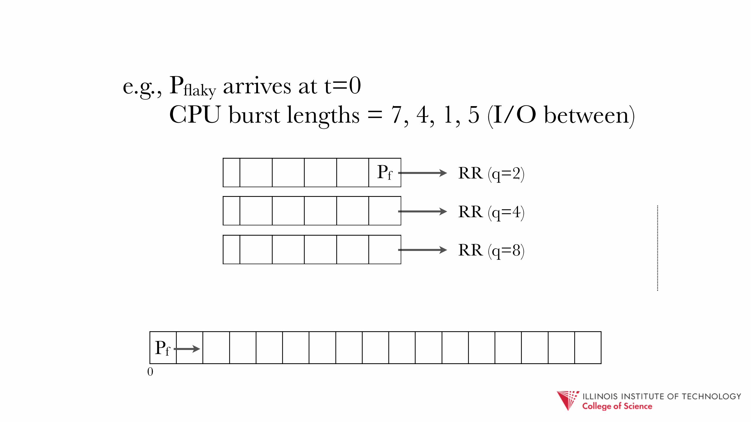
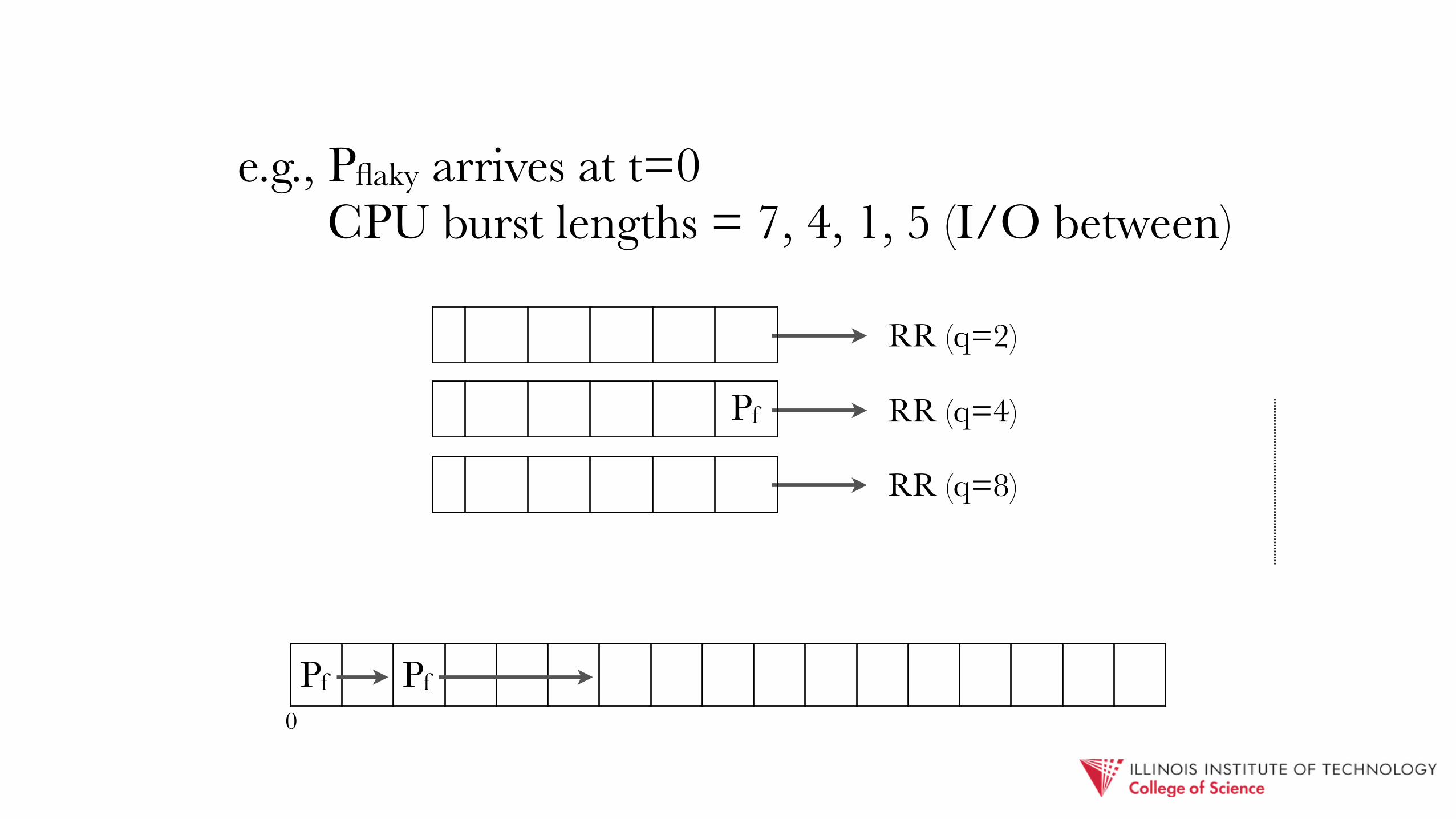
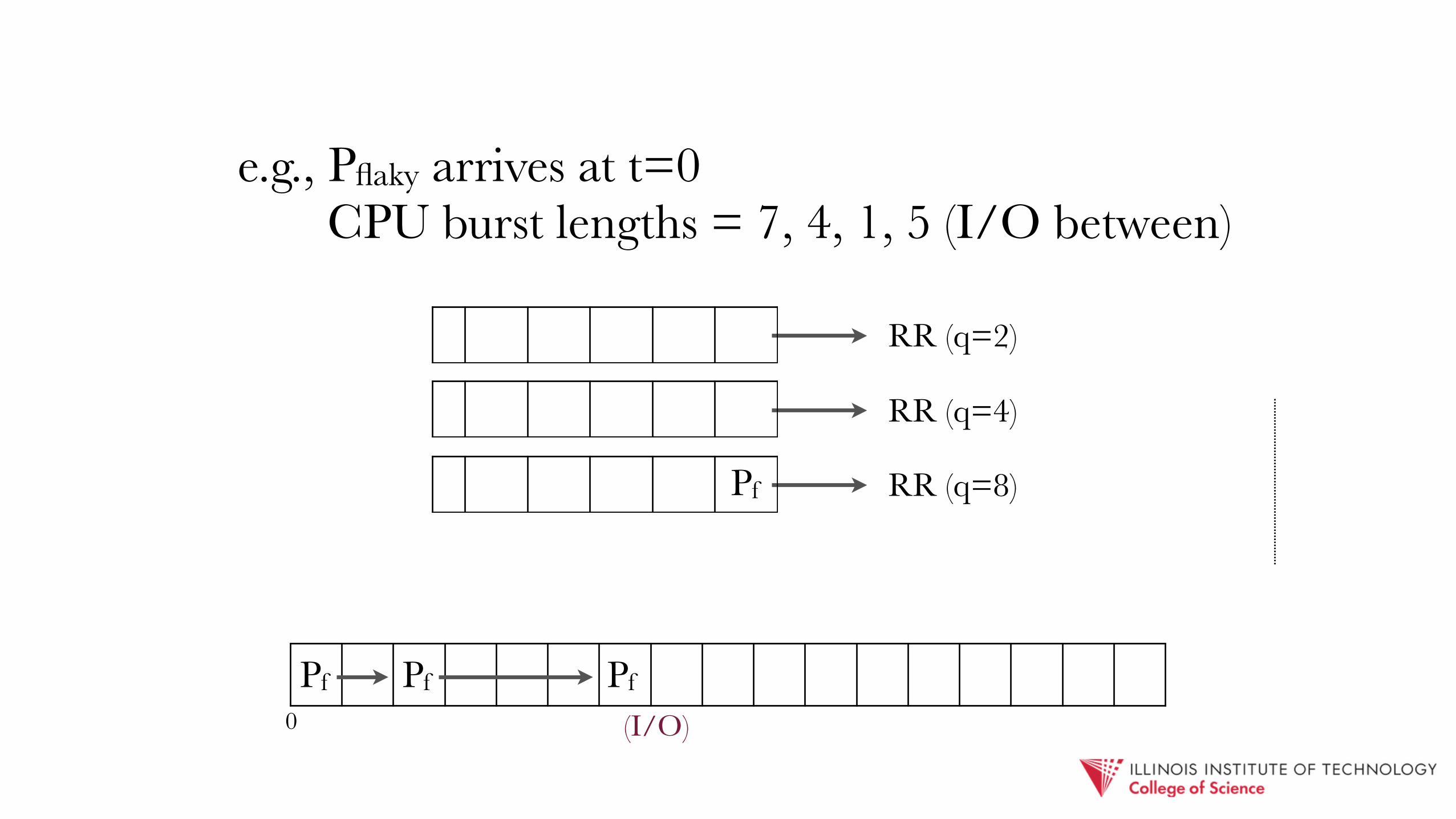
7. Multi-Level Feedback Queue (MLFQ) - supports movement between queues after initial assignment
- based on ongoing job accounting

RR (q=2)
RR (q=8)
RR (q=4)
e.g., 3 RR queues with different q
assignment based on q/burst-length fit

RR (q=2)
RR (q=4)
RR (q=8)
0
P1
P1
Process Arrival Time Burst TimeP1 0 7P2 2 4P3 4 1P4 5 4

RR (q=2)
P1 RR (q=4)
RR (q=8)
P10
P2
P2
Process Arrival Time Burst TimeP1 0 7P2 2 4P3 4 1P4 5 4

RR (q=2)
P2 P1 RR (q=4)
RR (q=8)
P10
P2
P3
P3
Process Arrival Time Burst TimeP1 0 7P2 2 4P3 4 1P4 5 4

RR (q=2)
P2 P1 RR (q=4)
RR (q=8)
P1 P30
P2
P4
P4
Process Arrival Time Burst TimeP1 0 7P2 2 4P3 4 1P4 5 4
RR (q=2)
P4 P2 P1 RR (q=4)
RR (q=8)
P1 P30
P2 P4 P1
Process Arrival Time Burst TimeP1 0 7P2 2 4P3 4 1P4 5 4
RR (q=2)
P4 P2 RR (q=4)
P1 RR (q=8)
P1 P30
P2 P4 P1 P2
Process Arrival Time Burst TimeP1 0 7P2 2 4P3 4 1P4 5 4

RR (q=2)
P4 RR (q=4)
P1 RR (q=8)
P1 P30
P2 P4 P1 P2 P4
Process Arrival Time Burst TimeP1 0 7P2 2 4P3 4 1P4 5 4

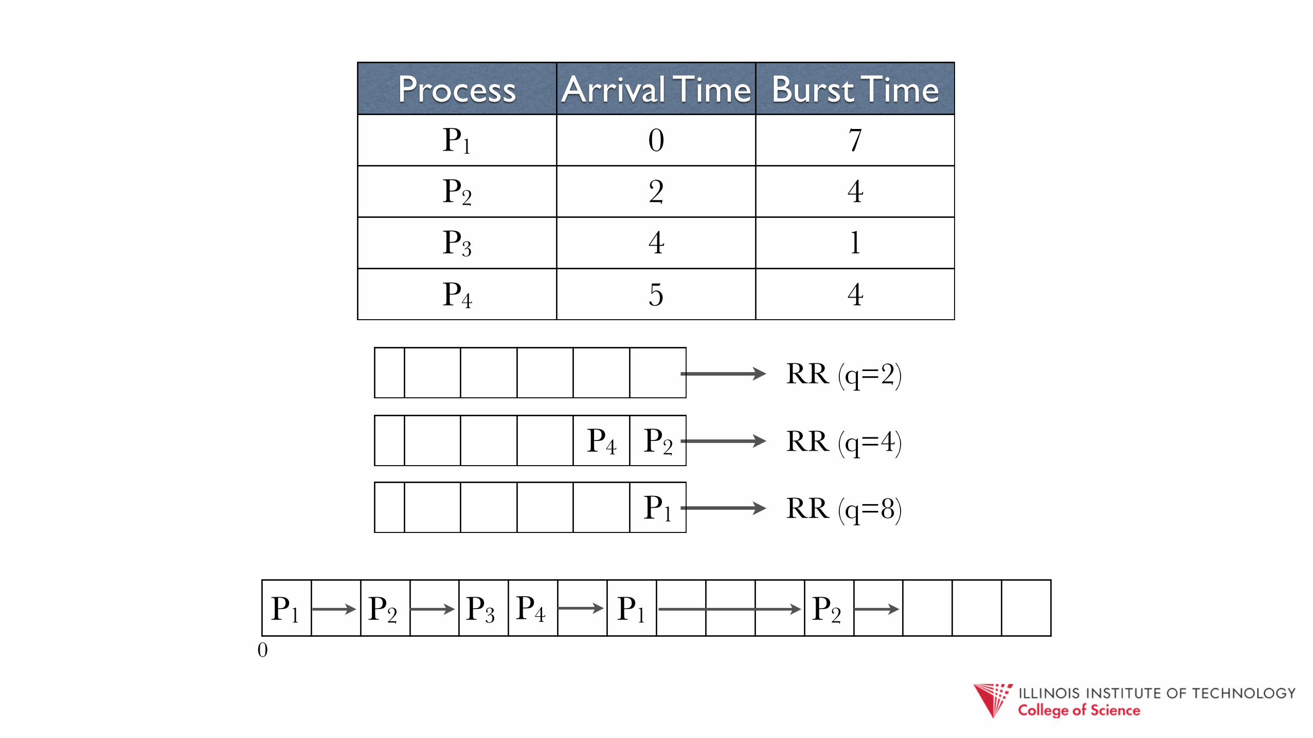
RR (q=2)
RR (q=4)
P1 RR (q=8)
P1 P30
P2 P4 P1 P2 P4 P1
Process Arrival Time Burst TimeP1 0 7P2 2 4P3 4 1P4 5 4
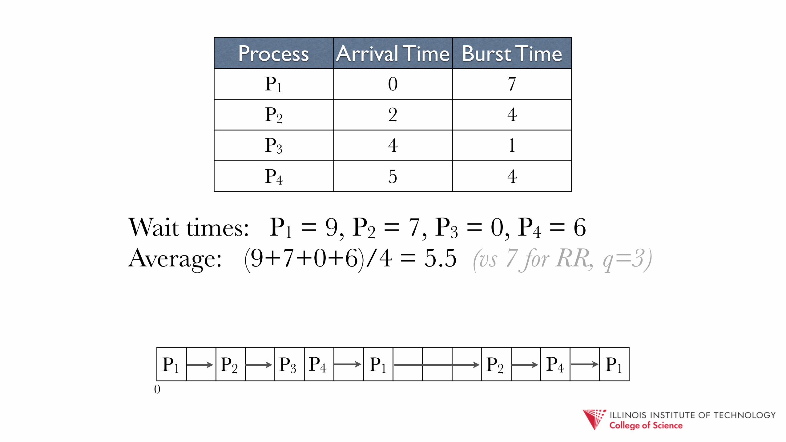
P1 P30
P2 P4 P1 P2 P4 P1
Wait times: P1 = 9, P2 = 7, P3 = 0, P4 = 6 Average: (9+7+0+6)/4 = 5.5 (vs 7 for RR, q=3)
Process Arrival Time Burst TimeP1 0 7P2 2 4P3 4 1P4 5 4

- following I/O, processes return to previously assigned queue - when to move up?
- for RR, when burst ≤ q

RR (q=2)
RR (q=4)
RR (q=8)
0
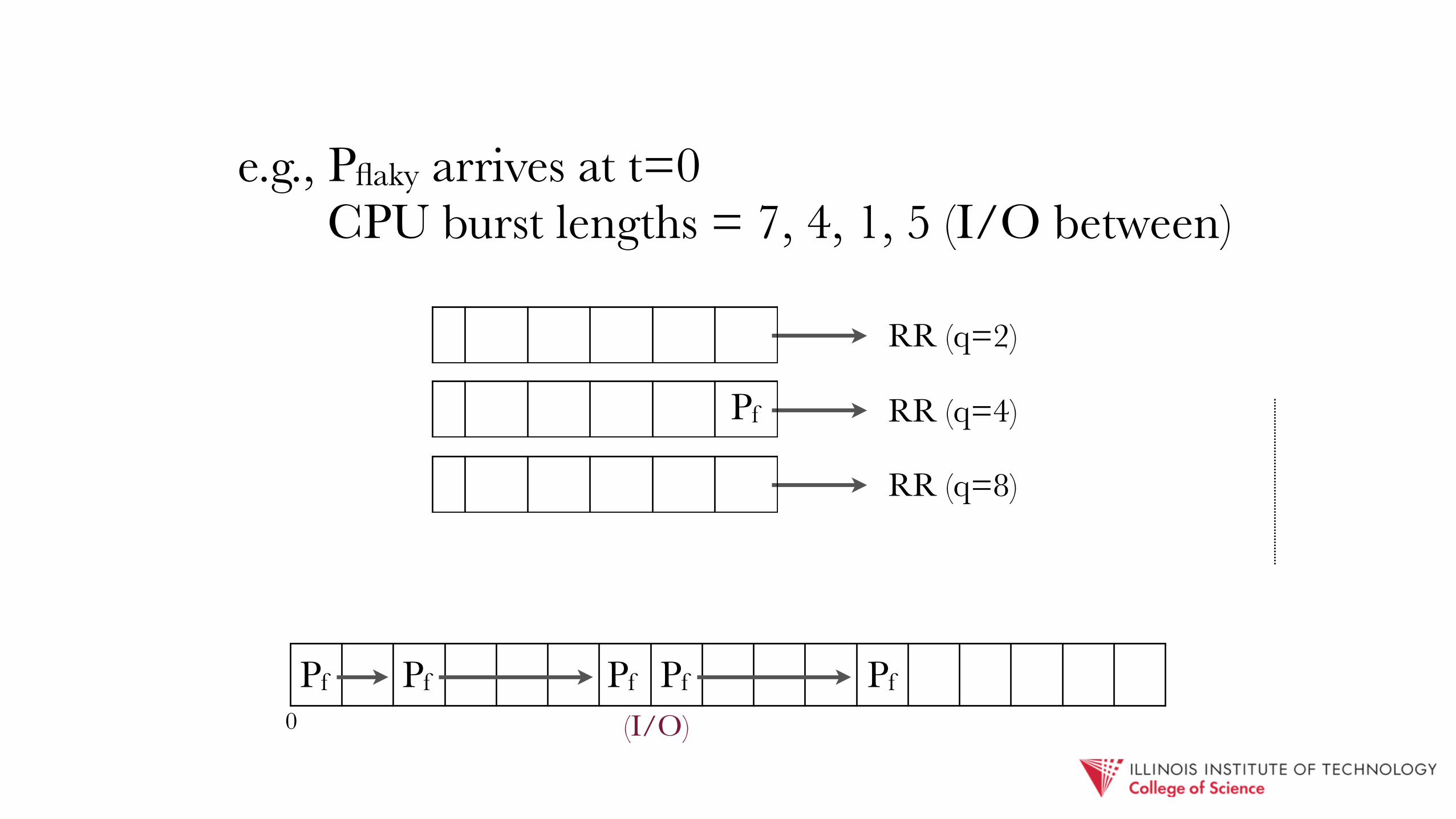
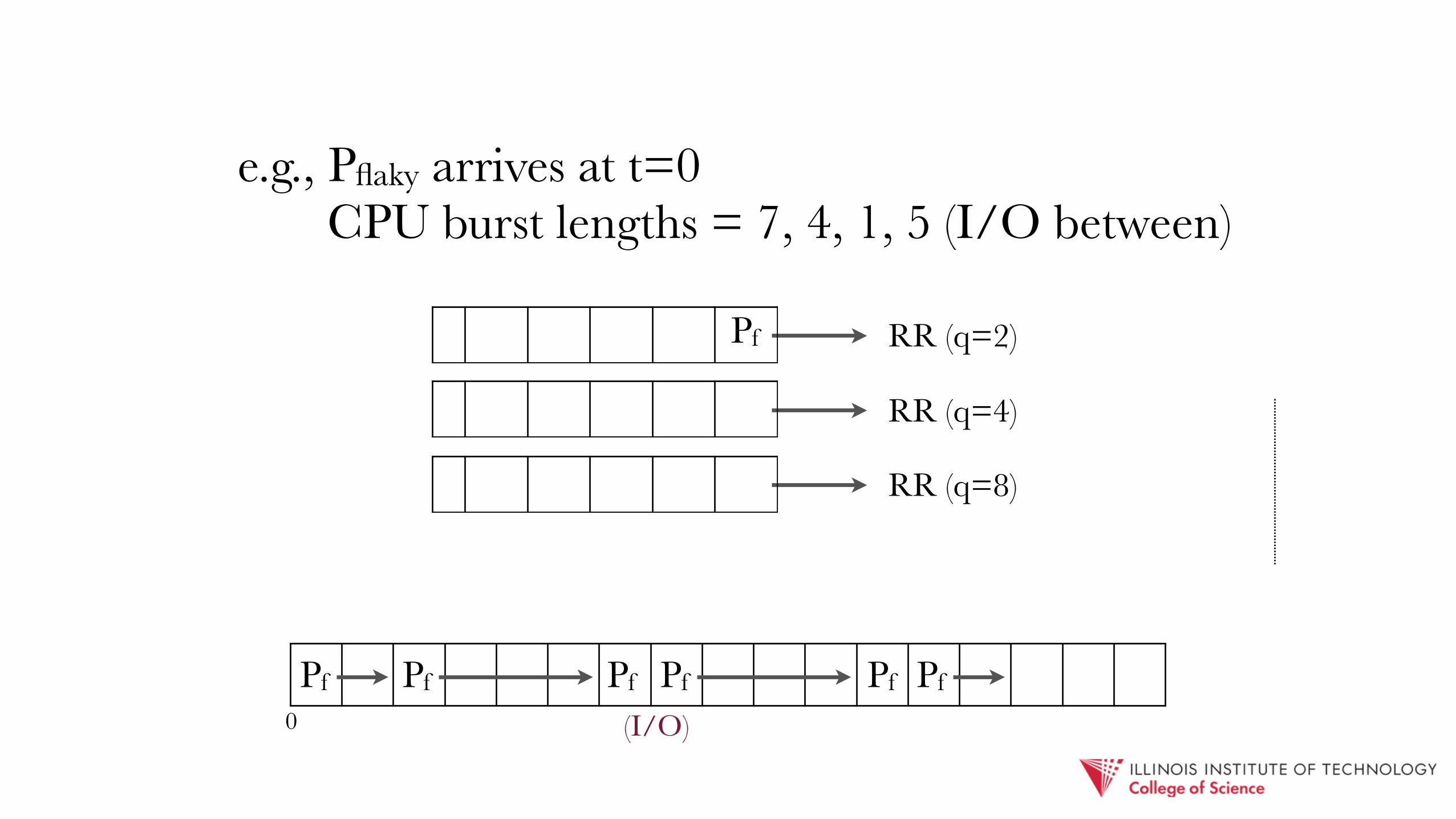
e.g., Pflaky arrives at t=0 CPU burst lengths = 7, 4, 1, 5 (I/O between)
RR (q=2)
RR (q=4)
RR (q=8)
0
e.g., Pflaky arrives at t=0 CPU burst lengths = 7, 4, 1, 5 (I/O between)
Pf
Pf
RR (q=2)
RR (q=4)
RR (q=8)
0
Pf
Pf Pf
e.g., Pflaky arrives at t=0 CPU burst lengths = 7, 4, 1, 5 (I/O between)

RR (q=2)
RR (q=4)
RR (q=8)
0
Pf Pf
Pf
Pf
e.g., Pflaky arrives at t=0 CPU burst lengths = 7, 4, 1, 5 (I/O between)
RR (q=2)
RR (q=4)
RR (q=8)
0
Pf
Pf Pf Pf
(I/O)
e.g., Pflaky arrives at t=0 CPU burst lengths = 7, 4, 1, 5 (I/O between)

RR (q=2)
RR (q=4)
RR (q=8)
0
Pf Pf Pf
(I/O)
e.g., Pflaky arrives at t=0 CPU burst lengths = 7, 4, 1, 5 (I/O between)

RR (q=2)
RR (q=4)
RR (q=8)
0
Pf Pf Pf
(I/O)
Pf
Pf
e.g., Pflaky arrives at t=0 CPU burst lengths = 7, 4, 1, 5 (I/O between)

RR (q=2)
RR (q=4)
RR (q=8)
0
Pf Pf Pf
(I/O)
Pf
Pf
e.g., Pflaky arrives at t=0 CPU burst lengths = 7, 4, 1, 5 (I/O between)

RR (q=2)
RR (q=4)
RR (q=8)
0
Pf Pf Pf
(I/O)Pf
e.g., Pflaky arrives at t=0 CPU burst lengths = 7, 4, 1, 5 (I/O between)
RR (q=2)
RR (q=4)
RR (q=8)
0
Pf Pf Pf
(I/O)Pf
Pf
Pf
e.g., Pflaky arrives at t=0 CPU burst lengths = 7, 4, 1, 5 (I/O between)

RR (q=2)
RR (q=4)
RR (q=8)
0
Pf Pf Pf
(I/O)Pf
Pf
Pf
e.g., Pflaky arrives at t=0 CPU burst lengths = 7, 4, 1, 5 (I/O between)

RR (q=2)
RR (q=4)
RR (q=8)
0
Pf Pf Pf
(I/O)Pf Pf
e.g., Pflaky arrives at t=0 CPU burst lengths = 7, 4, 1, 5 (I/O between)
RR (q=2)
RR (q=4)
RR (q=8)
0
Pf Pf Pf
(I/O)Pf Pf
Pf
Pf
e.g., Pflaky arrives at t=0 CPU burst lengths = 7, 4, 1, 5 (I/O between)

RR (q=2)
RR (q=4)
RR (q=8)
0
Pf Pf Pf
(I/O)Pf Pf
Pf
Pf Pf
e.g., Pflaky arrives at t=0 CPU burst lengths = 7, 4, 1, 5 (I/O between)

RR (q=2)
RR (q=4)
RR (q=8)
0
Pf Pf Pf
(I/O)Pf Pf Pf Pf
e.g., Pflaky arrives at t=0 CPU burst lengths = 7, 4, 1, 5 (I/O between)

other possible heuristics: - multi-queue hops due to huge bursts
- exponential backoff to avoid queue hopping
- dynamic queue creation for outliers

§ Scheduler Evaluation

i.e., how well does a given scheduling policy perform under different loads?
typically, w.r.t. scheduling metrics: wait time, turnaround, utilization, etc.

n.b., numerical metrics (e.g., wait time) are important, but may not tell the full story
e.g., how, subjectively, does a given scheduler “feel” under regular load?

1. paper & pencil computations
2. simulations with synthetic or real-world job traces
3. mathematical models; e.g., queueing theory 4. real world testing (e.g., production OSes)

(never fear, you’ll try your hand at all!)
e.g., UTSA process scheduling simulator - specify scheduling discipline and job details in configuration
file
- bursts can be defined discretely, or using probability distributions
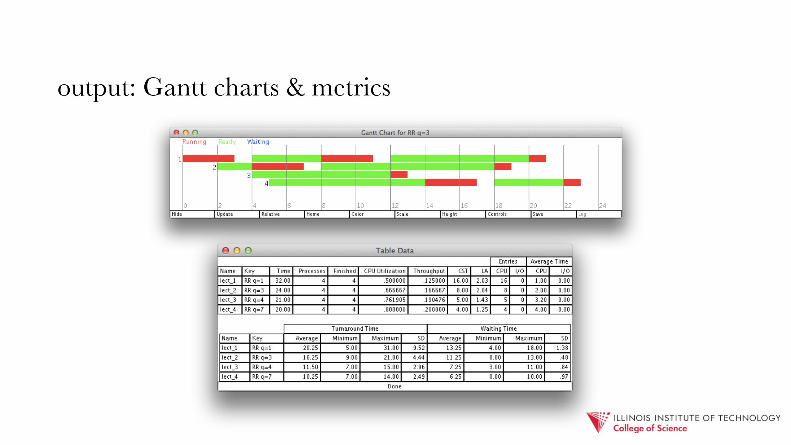
output: Gantt charts & metrics

SJF vs. PSJF vs. RR, q=10 vs. RR, q=20processes: uniform bursts ≤ 20, CST = 1.0
Which is which?


