Scheduling Second-Order

Computational Load in

Master-Slave Paradigm

S. SURESH, Senior Member, IEEE

Nanyang Technological University

CUI RUN

HYOUNG JOONG KIM, Member, IEEE

Korea University

THOMAS G. ROBERTAZZI, Fellow, IEEE

SUNY, Stony Brook

YOUNG-IL KIM

Korea Telecom

Scheduling divisible loads with the nonlinear computationalcomplexity is a challenging task as the recursive equations arenonlinear and it is difficult to find closed-form expression forprocessing time and load fractions. In this study we attempt toaddress a divisible load scheduling problem for computationalloads having second-order computational complexity in amaster-slave paradigm with nonblocking mode of communication.First, we develop algebraic means of determining the optimalsize of load fractions assigned to the processors in the networkusing a mild assumption on communication-to-computationspeed ratio. We use numerical simulation to verify the closenessof the proposed solution. Like in earlier works which considerprocessing loads with first-order computational complexity, westudy the conditions for optimal sequence and arrangementsusing the closed-form expression for optimal processing time.Our finding reveals that the condition for optimal sequenceand arrangements for second-order computational loads arethe same as that of linear computational loads. This schedulingalgorithm can be used for aerospace applications such as Houghtransform for image processing and pattern recognition usinghidden Markov model (HMM).

Manuscript received April 21, 2010; revised September 3 and

November 29, 2010; released for publication February 11, 2011.

IEEE Log No. T-AES/48/1/943648.

Refereeing of this contribution was handled by L. Kaplan.

The work of S. Suresh was supported by NTU-SUG program by

Nanyang Technological University. The work of H-J. Kim was

supported by the IT R&D program (ITRC), the CTRC program of

MCST/KOCCA, Korea University, and the 3DLife project by the

National Research Foundation. The work of T. G. Robertazzi was

supported by DOE Grant DE-SC0003361.

Authors’ addresses: S. Suresh, School of Computer Engineering,

Nanyang Technological University, #02b-67, Bik N4, Singapore,

637820, Singapore, E-mail: (ssundaram@ntu.edu.sg); C. Run and

H. J. Kim, CIST, Graduate School of Information Management

and Security, Korea University, Seoul 136-701, Korea; T. G.

Robertazzi, Department of Electrical and Computer Engineering,

State University of New York at Stony Brook, Stony Brook, NY

11794-2350; Y-I. Kim, Korea Telecom, KT Central R&D Center,

Seoul 137-792, Korea.

0018-9251/12/$26.00 c° 2012 IEEE

I. INTRODUCTION

Researchers are producing a huge amount of data

to solve complex and interdisciplinary problems.

The efforts to solve such complex problems are

hindered by time-consuming postprocessing in

a single workstation. Data-driven computation

is an active area of research, which addresses

the issue of handling huge data sets. The main

objective in data-driven computation is to minimize

the processing time of computing loads by using

distributed computing system. These computing

loads are assumed to be divisible arbitrarily into

small fractions and processed independently in the

processors. The above assumption on computing loads

is suitable for many practical applications involving

data parallelism such as image processing, pattern

recognition, bio-informatics, data mining, etc. The

main thrust in the parallel processing of divisible

loads is to design efficient scheduling algorithms that

minimize the total load processing time. The domain

of scheduling divisible loads in a multiprocessor

system is commonly referred as divisible load theory

(DLT) and is of interest to researchers in the field of

scheduling loads in computer networks. The problem

of scheduling divisible loads in intelligent sensor

networks started in 1988 by Cheng and Robertazzi

[13]. Here, an intelligent sensor network with

master-slave architecture is considered where a master

processor can measure, compute, and communicate

with other intelligent sensors for collaborative

computing.

The first mathematical model considered [13]

is similar to a linear network of processors. The

optimal load allocation strategy presented in [13] is

extended to tree networks in [14] and bus networks

in [11], [34]. An optimal load allocation for linear

network of processors is presented by the theory

that all processors stop computing at the same time

instant [13]. In fact, this condition has been shown to

be a necessary and sufficient condition for obtaining

optimal processing time in linear networks [33]

by using the concept of processor equivalence. An

analytical proof of this assumption in bus networks is

presented in [35]. This assumption has been proven in

a rigorous manner and it is shown that this assumption

is true only in a restricted sense [8]. The concepts

of optimal sequencing and optimal arrangement are

introduced [4, 29] and parameters for computation

and communication are probed for adaptive distributed

processing [22].

Since 1988 research works [6—8, 11—14, 17—20,

22, 25, 29, 33—37, 41] in DLT framework have been

carried out by algebraic means to determine optimal

fractions of a load distributed to processors in the

network such that the total load processing time is

minimum. A number of scheduling policies have

been investigated including multi-installments [5],

780 IEEE TRANSACTIONS ON AEROSPACE AND ELECTRONIC SYSTEMS VOL. 48, NO. 1 JANUARY 2012

multi-round scheduling [7, 42], multiple loads [17],

limited memory [20, 38], simultaneous distribution

[24, 32], simultaneous start [36], start-up delay

[9, 39], detailed parameterizations and solution

time optimization [1], and combinatorial schedule

optimization [21]. Divisible loads may be divisible

in fact or as an approximation as in the case of a

large number of relatively small independent tasks

[3, 10]. Ten reasons to use the concept of divisible

load scheduling theory have recently been presented

[34]. Results and open problems in divisible load

scheduling in single level tree network are highlighted

in [6]. A complete survey and results in divisible

load scheduling algorithm can be found in [8], [34],

[36]. The aforementioned research works in the

domain of divisible load scheduling in distributed

systems consider processing load requiring linear

computational power.

There is an increasing amount of research on

real-time modeling and simulation of complex

systems such as nuclear modeling, aircraft/spacecraft

simulation, biological systems, bio-physical

modeling, genome search, etc. It is well known that

many algorithms require nonlinear computational

complexity, i.e., the computational time of the given

data/load is a nonlinear function of the load size

(N). For the first time in the literature, a nonlinear

cost function is considered [19, 25]. In [25] the

computational loads require nonlinear processing time

depending on the size of load fractions. It has been

mentioned that because of nonlinear dependency the

speed-up achieved by simultaneous-start is superlinear

[19, 25]. Finding an algebraic solution for nonlinear

computational loads is a challenging issue. In this

paper we present an approximate algebraic solution

for second-order computational loads.

Image processing and pattern analysis for

aerospace applications of which computational

complexity is O(N2) include line detection using

the Hough transform [15], and pattern recognition

using 2D hidden Markov model (HMM) [31]. The

classical Hough transform was concerned with the

identification of lines in the image, but later this

transform was extended to identifying positions of

arbitrary shapes, most commonly circles or ellipses.

The computational complexity for N points is

approximately proportional to N2. When N is large,

parallel or distributed processing is desired [23]. A

separable 2D HMM for face recognition builds on

an assumption of conditional independence in the

relationship between adjacent blocks. This allows

the state transition to be separated into vertical and

horizontal state transitions. This separation of state

transitions brings the complexity of the hidden layer

of the proposed model from the order of O(N3k)

to the order of O(N2k), where N is the number of

the states in the model and k is the total number of

Fig. 1. Master-slave network.

observation blocks in the image [23]. In addition,

we can also find real-world problems like molecular

dynamic simulation of macromolecular systems,

learning vector quantization neural network [27],

and block tri-diagonalization of real symmetric

matrices [2] which require second-order computational

complexity.

In this paper we address the scheduling problem

for second-order computational loads in a master-slave

paradigm with nonblocking mode communication.

Here the second-order time complexity computational

load arrives at the master processor and it distributes

the load fractions one-by-one to the slave processors

in the network using the nonblocking mode of

communication. Using a mild assumption on the

communication to computation speed ratio and

the minimum granularity of any load fractions, we

derive an algebraic solution for the optimal size of

the each load fraction and the total load processing

time. Numerical solutions are compared with the

algebraic solution to see if they conform to each

other. The results clearly indicate that the algebraic

closed-form expression matches closely with the

numerical solution. Finally, we study the conditions

for optimal sequence and optimal arrangement using

the closed-form expression. Our finding reveals that

the condition for optimal sequence/arrangements is the

same as that of linear computational loads.

II. MATHEMATICAL FORMULATION

In this section, we describe the master-slave

model and formulate the problem. We consider a

second-order computational load which is arbitrarily

divisible. The user submits the computational load

in the master processor (p0). The master processor

p0 is connected to m slave processors (p1,p2, : : : ,pm)

through the links (l1, l2, : : : , lm) as shown in Fig. 1.

The root processor (p0) divides the processing load

into m+1 fractions (®0,®1, : : : ,®m), keeps ®0 for

itself and distributes the remaining m fractions to

child processors (p0,p1,p2, : : : ,pm) in the network.

The processing time to compute the load fraction

depends linearly on the computing speed of the

processor and nonlinearly in terms of the size of load

fraction. In this paper we use nonblocking mode of

SURESH, ET AL.: SCHEDULING SECOND-ORDER COMPUTATIONAL LOAD IN MASTER-SLAVE PARADIGM 781

Fig. 2. Timing diagram describing load distribution process in master-slave network.

communication [28, 40] to distribute the load fractions

(®0,®1, : : : ,®m) to slave processors (p1,p2, : : : ,pm). In

the nonblocking mode of communication, the child

processor will start the computation process while

its front-end starts receiving the fraction of loads.

The objective of this study is to find the optimal

size of load fractions assigned to the processors in

the network such that the total processing time is

minimum. The following are the notations used in this

paper.

®0 Fraction of the load assigned to the root

processor p0.

®i Fraction of the load assigned to the child

processor pi.

Ai Inverse computing speed on the processor pi.

Gi Inverse link speed on the link li.

T(m) Total time taken to process the complete load.

N Total size of the load fractions.

m Number of the slave processors.

n Order of processing.

± Minimum granularity of any load fraction.

A. Optimal Load Scheduling

We derive the closed-form expressions for the

load fractions and processing time for nonlinear

processing load in the nonblocking mode of

communication model. For the purpose of derivation

of the closed-form expression, we consider a sequence

of load distribution, p1,p2, : : : ,pm, in that order.

The problem is to find the optimal sizes of the

load fractions that are assigned to the processors in

the network such that the final processing time is

minimal. The load distribution process by the master

processor p0 is illustrated by means of a timing

diagram as shown in Fig. 2. As in the case of linear

computational loads [8], the processing time for

nonlinear computational loads is minimum only when

all processors stop computing at the same time. The

detailed proof for second-order computational loads is

given in the Appendix.

From the timing diagram, we can write the

recursive load distribution equations as follows:

(®1N)nA1 = (®oN)

nA0 (1)

(®i+1N)nAi+1 + (®iN)Gi = (®iN)

nAi,

i = 1,2, : : : ,m¡ 1: (2)

The above equations are reduced to

(®1N)n = (®oN)

nf1, (3)

(®i+1N)n = (®iN)

nfi+1¡ (®iN)¯ifi+1,i= 1,2, : : : ,m¡ 1 (4)

where

fi+1 =AiAi+1

, i= 0,1,2, : : : ,m¡ 1 (5)

¯i =GiAi, i= 1,2, : : : ,m¡ 1: (6)

The normalization equation is

mXi=0

®i = 1: (7)

Equations (3) and (4) can be reduced to

ga1N = ®0Nnpf1 (8)

gai+1N = ®iNnpfi+1

·1¡ ¯i

(®iN)n¡1

¸1=n,

i = 1,2, : : : ,m¡ 1: (9)

782 IEEE TRANSACTIONS ON AEROSPACE AND ELECTRONIC SYSTEMS VOL. 48, NO. 1 JANUARY 2012

The size of load fractions can be obtained

by substituting (8) and (9) in (7) and solved

analytically. Solving these equations is difficult and

computationally intensive. In this paper we derive a

closed-form expression for the size of load fraction

and processing time by approximating the terms inside

the root. Finding approximate closed-form expression

for higher power is difficult. Hence, in this paper

we consider only the second power (n= 2). If we

substitute n with 2 in (8) and (9), then the equations

are reduced as

®1N = ®0Npf1 (10)

®i+1N = ®iNpfi+1

s1¡ ¯i

®iN, i= 1,2, : : : ,m¡ 1:

(11)

Assumption: We assume that the ratio of

communication time to computation (¯i) is very small

in most practical distributed systems. Also, the size

of load fraction assigned to the child processor ®iN is

larger than ¯i.

Using the above assumption, we express the term

(p1¡¯i=®iN) in (11) in Taylor series ass

1¡ ¯i®iN

= 1¡ ¯i(®iN)

+O

Ãμ¯i®iN

¶2!: (12)

Note that the communication-to-computation ratio

(¯i) is less than 1 and the load fraction assigned

to the child processor is greater than the minimum

granularity of processing load (®iN > ±). Hence,

the higher order terms of ¯i=®iN are small and are

neglected.

In this paper we consider a first-order

approximation of square root to derive the

closed-form expression.s1¡ ¯i

®iN¼ 1¡ ¯i

2®iN: (13)

The approximation holds only when ¯i=®iN is much

smaller than one and ¯i=®iN moves closer to ¯i=±,

the approximation become worse. By substituting

the approximation of the square root, (11) can be

simplified as

®i+1N ¼ ®iNpfi+1¡

¯ipfi+12

, i= 1,2, : : : ,m¡1:

(14)

By substituting (14) and (10) in normalization (7),

we can derive the closed-form expression for the load

fraction ®0 assigned to the root processor p0 as

®0 =N + x(m)

Ny(m)(15)

where

x(m) =1

2

m¡1Xi=1

¯i

24 mXj=i+1

jYk=i+1

pfk

35 (16)

y(m) = 1+

24 mXi=1

iYj=1

qfj

35 : (17)

From (10) and (15), the load fraction ®i can be

expressed in terms of load fraction ®0 as

®iN ¼ ®0Npf1f2 ¢ ¢ ¢fi¡

1

2

i¡1Xj=1

¯j

iYk=j+1

pfk,

i= 1,2, : : : ,m: (18)

By substituting the closed-form expression for load

fraction ®0 in (18), one can easily calculate the size of

load fraction assigned to any processor in the network

as follows:

®i =1

N

24N + x(m)y(m)

pf1f2 ¢ ¢ ¢fi¡

1

2

i¡1Xj=1

¯j

iYk=j+1

pfk

35 ,i= 1,2, : : : ,m: (19)

Now we derive the closed-form expression for the

total load processing time. From the timing diagram

shown in Fig. 2, the total load processing time T(m) is

given as follows:

T(m) = (®0N)2A0 =

·N + x(m)

y(m)

¸2A0: (20)

One should remember that the above closed-form

expression for processing time is derived under the

assumption that the communication time is less than

the computation time. When the communication

time is greater than the computation time (¯i > 1),

simultaneous processing is not possible. The processor

will have cycles of the work and wait period. For

this case, finding closed-form expression is not

straightforward. This case can be handled easily

using the equivalent processor concept explained in

[28], [40].

The advantage of the closed-form expression

is that we can directly derive conditions for the

optimal sequence of load distribution and the optimal

arrangement of processors. Before analyzing the

theoretical results, we present a numerical example to

understand the characteristics of nonlinear DLT with

nonblocking mode of communication.

B. Numerical Example 1

Consider the task of finding ellipses in a 512£ 512image. Lets assume that the ellipses are oriented

along the principle axes. Hence, we need four

parameters (k = 4) (two for the center of the ellipse

and two for the radii) to describe the ellipse. The

SURESH, ET AL.: SCHEDULING SECOND-ORDER COMPUTATIONAL LOAD IN MASTER-SLAVE PARADIGM 783

TABLE I

Processor and Communication Link Parameters used in the

Numerical Example 1

Parameters P0 P1 P2 P3

A 900 800 120 100

G – 20 1 0.85

computational complexity in identifying the ellipse

is O(Nk¡2), which is O(N2). Here, N is image space

(N = 262144). For simplicity we consider a small

region of interest 10£ 10 (N = 100) in our example.The root processor divides the image size into small

fractions and distributes them to child processors.

Each child processor computes the Hough space for

a given resolution and generates the accumulator

array for their fraction of image region. The size

of accumulator array depends on the resolution and

does not depend on the image size. Finally, the root

processor collects all the arrays and identifies the

candidate points for ellipses. For simplicity we neglect

the result collection time (resolution is much smaller

than image size) from each processor.

Consider a single-level tree network with

three processors (m= 3). The time to compute the

accumulator array for one pixel (processors parameter)

and the time to communicate one pixel through the

link (link parameters) are given in Table I. The total

size of load fraction N is assumed to be 100 units.

Using the closed-form expression, the values of

fractions assigned to the processors are computed as

follows: ®0 = 0:12840, ®1 = 0:13619, ®2 = 0:35132,

and ®3 = 0:38480. The corresponding total load

processing time is 148,384 units of time. The total

load processing time obtained by analytically solving

the nonlinear recursive equations using a nonlinear

least square solver [16] is 148,170 units of time. The

load fractions obtained using the analytical solution

are: ®0 = 0:128309, ®1 = 0:13609, ®2 = 0:351068,

and ®3 = 0:38453. From the results we can see that

the closed-form expressions closely approximate the

actual solution.

The processing time obtained using the

closed-form expression and actual solution obtained

using the analytical solution are given in Table II.

From the table we can see that the processing time

obtained using the approximate closed-form solution

matches with the analytical solution. The difference

between the solutions depends on the ratio between

communication time to computation time (¯i) and size

of load fraction (®iN). The error is small when ¯i=®iN

is close to zero and it becomes worse when ¯i=®iN

moves closer to ¯i=±.

The main objective of deriving the closed-form

expression is to study the behavior of second-order

load scheduling problems. In the following section

we show that the approximate closed-form solution

TABLE II

Total Load Processing Time Obtained using Analytical Solution of

Recursive Equations and Approximate Closed-Form Expression

# of Child Approximate Analytical

Processors Solution Solution

1 2,119,482 2,119,482

2 391,247 390,995

3 148,384 148,170

can be directly used to find the conditions for

optimal arrangements and optimal sequence of load

distribution.

C. Homogeneous System

As a special case for the homogeneous system

(Ai = A and Gi =G), the load fraction assigned to the

root processor (®0) is obtained by substituting fi = 1

and ¯i = ¯ in (15) as follows:

®0 =4N +m¯(m¡ 1)4N(m+1)

: (21)

The load fraction assigned to any child processor

pi is obtained as follows:

®i =4N +m¯(m¡1)4N(m+1)

¡ (i¡ 1)¯2N

, i= 1,2, : : : ,m:

(22)The total load processing time for the

homogeneous system is computed as follows:

T(m) =

·4N +m¯(m¡ 1)

4(m+1)

¸2A: (23)

In the homogeneous case, if the

communication-to-computation ratio tends to be zero,

the load fractions assigned to the processors converge

to equal load fraction, i.e.,

®0 = lim¯!0

4N +m¯(m¡ 1)4N(m+1)

=1

m+1(24)

and

®i = lim¯!0

·4N +m¯(m¡ 1)4N(m+1)

¡ (i¡ 1)i¯2N

¸=

1

m+1,

i= 1,2, : : : ,m (25)

and the total load processing time converges to

T(m) =

·N

m+1

¸2A: (26)

From (26), we can see that the total processing time is

superlinear with increase in the number of processors.

III. OPTIMAL SEQUENCE OF LOAD DISTRIBUTION

In the linear DLT, the closed-form expression is

used to find the condition for the optimal sequence

of load distribution. Similarly, one needs to derive

the closed-form expression to study the behavior of

784 IEEE TRANSACTIONS ON AEROSPACE AND ELECTRONIC SYSTEMS VOL. 48, NO. 1 JANUARY 2012

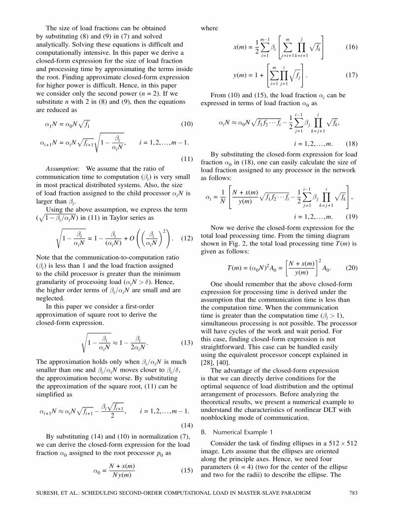
the nonlinear divisible load condition. In this sectionwe present the condition for optimal sequence ofload distribution obtained from the approximateclosed-form expression. First, we present an exampleto understand the effect of changing the sequence ofload distribution and later generalize the result. Forthis purpose we consider a three-processor (m= 3)network. From (20) we can see that the processingtime is a function of load fraction ®0 assigned to theprocessor p0. Hence, it is sufficient to analyze thebehavior of ®0 instead of processing time T(m).Case A: The sequence of load distribution is

(p1,p2,p3), i.e., the root processor p0 first sends theload fraction to the processor p1, next to the processorp2, and last to the processor p3. Using the closed-formexpression, we can write ®0 as

®0N =N +¯1

¡pf2 +

pf2f3

¢=2+¯2

¡pf3¢=2

1+pf1 +

pf1f2 +

pf1f2f3

:

(27)

The above equation can be expressed in terms ofsystem parameters (Ai,Gi) as

®0N =2NpA1A2A3 +G1

¡pA2 +

pA3

¢+G2

pA1

2¡p

A1A2A3 +pA0A2A3 +

pA0A1A3 +

pA0A1A2

¢ :(28)

Case B: Now, we change the load distributionsequence as (p1,p3,p2), i.e., the root processor p0 firstsends the load fraction to the processor p1, next, tothe processor p3 and finally to the processor p2. Theload fraction (®00) can be obtained by interchanging(A2,G2) and (A3,G3) in the earlier expression.

®00N =2NpA1A2A3 +G1

¡pA2 +

pA3

¢+G3

pA1

2¡p

A1A2A3 +pA0A2A3 +

pA0A1A3 +

pA0A1A2

¢ :(29)

Now, we have to find the condition for ®0 · ®00.By subtracting (29) and (28), we get

®0N ¡®00N

=

pA1(G2¡G3)

2¡p

A1A2A3 +pA0A2A3 +

pA0A1A3 +

pA0A1A2

¢ :(30)

From the above equation, we can say that the totalload processing time is minimal for load distributionsequence (p1,p2,p3) if and only if G2 is less thanG3. From the results obtained for the three-processornetwork case, we can generalize the result as follows.

Optimal Sequencing Theorem Given an(m+1)-processor single-level tree network withnonblocking mode of communication, the optimalsequence of load distribution is produced if the rootprocessor distributes the load fractions in ascendingorder of communication speed parameter Gi of thelinks.

PROOF For m processors, consider a case when

the root processor p0 distributes the load fractions

to child processors in the following sequence

(p1,p2, : : : ,pi¡1,pi,pi+1, : : : ,pm). The value of loadfraction ®0 assigned to the root processor for this

sequence is

®0 =N + x(m)

Ny(m): (31)

Consider another sequence of load distribution

where the root processor distributes the load

fractions to child processors in a sequence

(p1,p2, : : : ,pi¡1,pi+1,pi, : : : ,pm). The value of loadfractions assigned to the root processor in this

sequence is

®00 =N + x0(m)Ny0(m)

: (32)

The load fraction for the new sequence can be

obtained by exchanging the (Gi,Ai) and (Gi+1,Ai+1)

in (31). The interchange affects terms fi, fi+1, fi+2,

¯i, and ¯i+1 only, and does not affect the other terms.

Note that because of this interchange, y(m) and y0(m)will not change. Now, we will find the conditions for

®0 · ®00, which is the same as x(m)· x0(m). The termsx(m) and x0(m) are a function of f and ¯.

x(m) =1

2

8>><>>:¯1

£pf2 +

pf2f3 + ¢ ¢ ¢+

pf2f3 ¢ ¢ ¢fm

¤+ ¢ ¢ ¢

+¯i£p

fi+1 +pfi+1fi+2 + ¢ ¢ ¢+

pfi+1fi+2 ¢ ¢ ¢fm

¤+ ¢ ¢ ¢+¯m¡1

pfm

:

(33)Now, x(m)¡ x0(m) is given as follows:

x(m)¡ x0(m) = Gi¡Gi+12pAiAi+1

: (34)

Then,

®0N ¡®00N =Gi¡Gi+1

2y(m)pAiAi+1

: (35)

Here, note that ®0N · ®00N only when Gi ·Gi+1.By recursively applying the above condition, we can

get the optimal load distribution sequence which

satisfies the condition G1 ·G2 · ¢¢ ¢ ·Gm. This provesthe theorem.

The result obtained from the optimal sequencing

theorem is similar to that of the optimal sequence of

load distribution presented for the linear case [8, 29].

A. Numerical Example 2

In this example we consider the same parameters

used in the numerical example 1. In the previous

example, we used load distribution sequence

(p1,p2,p3). The total load processing time is

148,384 units. By applying the optimal sequencing

theorem, the optimal sequence of load distribution

is (p3,p2,p1). The load fractions assigned to the

processors in the network are ®0 = 0:128236, ®1 =

0:136015, ®2 = 0:351175, and ®3 = 0:38465. The

SURESH, ET AL.: SCHEDULING SECOND-ORDER COMPUTATIONAL LOAD IN MASTER-SLAVE PARADIGM 785

total load processing time is 148,000 units. From this

result, we can see that the total processing time for

the optimal sequence is less than that for the previous

sequence.

IV. OPTIMAL ARRANGEMENT OF PROCESSORS

In this section we derive the condition for the

optimal arrangement of processors in the nonlinear

divisible load problem using our closed-form

expressions. First we present an example to

understand the effect of changing the processor

arrangement and later generalize the result. For

this purpose, we consider a three-processor (m= 3)

network. Here, the sequence of load distribution is

fixed as (p1,p2,p3).

Case A: The processor p1 is connected to link l1,

processor p2 is connected to link l2, and processor

p3 is connected to link l3. Using our closed-form

expression, we can write ®0 as (28).

Case B: Now we change the arrangement of

processors in the network. The processor p1 is

connected to link l2 and the processor p2 is connected

to link l1. The load fraction (®00) can be obtained by

interchanging A1 and A2 in the earlier expression

as (28).

®00N =2NpA1A2A3 +G1

¡pA1 +

pA3

¢+G2

pA2

2¡p

A1A2A3 +pA0A2A3 +

pA0A1A3 +

pA0A1A2

¢ :(36)

Now we have to find the condition for ®0 · ®00. Bysubtracting (28) and (36), we get

®0N ¡®00N

=

¡pA1¡

pA2

¢(G2¡G1)

2¡p

A1A2A3 +pA0A2A3 +

pA0A1A3 +

pA0A1A2

¢ :(37)

From the above equation, we know that the

processing time is a minimum if and only if the

sequence of load distribution based on ascending

order of communication speed parameter, i.e., G1 ·G2. Hence, from the above equation, we can change

the arrangement if and only if the processing speed

A2 is less than A1. Now, we generalize the result as

follows:

Optimal Arrangement Theorem Given an

(m+1)-processor single-level tree network with

optimal sequence of load distribution, the total load

processing time is minimum if the processors are

connected to the links in ascending order of processor

speed parameter Ai.

PROOF For m processors, consider a case when

the root processor p0 distributes the load fractions

to child processors in the following sequence

(p1,p2, : : : ,pi¡1,pi,pi+1, : : : ,pm). Here the networkarrangement

is (p1, l1), (p2, l2), : : : , (pi, li), (pi+1, li+1), : : : , (pm, lm).

The value of load fraction ®0 assigned to the root

processor in this arrangement is given as (31).

Consider another arrangement where a processor

pi is connected to a link li+1 and a processor pi+1is connected to a link li, i.e., the arrangement is

(p1,p2, : : : ,pi¡1,pi,pi+1, : : : ,pm). Here the networkarrangement is

(p1, l1), (p2, l2), : : : , (pi+1, li), (pi, li+1), : : : , (pm, lm). The

value of load fractions assigned to the root processor

in this arrangement is given as (32).

The load fraction for the new arrangement can

be obtained by exchanging the Ai and Ai+1 in (31).

The interchange affects terms fi, fi+1, fi+2, ¯i, and

¯i+1 only, and does not affect the other terms. Note

that because of this interchange, y(m) and y0(m) willnot change. Now, we find the conditions for ®0 · ®00which is the same as x(m)· x0(m). The terms x(m)and x0(m) are a function of fs and ¯s.Now, x(m)¡ x0(m) is given as follows:

x(m)¡ x0(m)

=(Gi+1¡Gi)

¡pAi¡

pAi+1

¢nPm

j=i+2

Qj

k=i+2

pfk

o2pAiAi+1

:

(38)Then,

®0N ¡®00N

=(Gi+1¡Gi)

¡pAi¡

pAi+1

¢nPm

j=i+2

Qj

k=i+2

pfk

o2y(m)

pAiAi+1

:

(39)

Here, note that ®0N · ®00N only when Ai · Ai+1.By recursively applying the above condition, we can

get the optimal load distribution sequence which

satisfies the condition A1 · A2 · ¢¢ ¢ · Am. This provesthe theorem.

In the above analysis, the speed condition of the

root processor is not included. Now, we prove the

speed condition on the root processor.

Let us consider a two-processor network and

the arrangement of processors in the network is

(p1, l1) and (p2, l2). The processing time for this

arrangement is

T =

(2NpA1A2 +G1

2¡pA1A2 +

pA0A1 +

pA0A2

¢)2A0: (40)Now, assume that the processor p1 should

distribute the load fractions instead of processor p0.

Then, we have to consider another arrangement:

(p0, l1) and (p2, l2). The total load processing time for

this arrangement is

T0 =

(2NpA0A2 +G1

2¡pA0A2 +

pA1A0 +

pA1A2

¢)2A1: (41)786 IEEE TRANSACTIONS ON AEROSPACE AND ELECTRONIC SYSTEMS VOL. 48, NO. 1 JANUARY 2012

Fig. 3. Timing diagram for load distribution process (m= 3).

The value T¡T0 is computed as follows:T¡T0

=G1

£4NpA0A1A2 +G1

¡pA0 +

pA1

¢¤2¡p

A0A1 +pA0A2 +

pA1A2

¢2 ³pA0¡

pA1

´:

(42)

Hence, T · T0 only when A0 · A1. From here we

can say that the first processor should be fastest. Note

that to find the speed condition of the root processor,

we have to use the processing time expression. For the

speed condition of the child processors, it is sufficient

to consider the value of the ®0 expression rather than

the processing time expression.

A. Numerical Example 3

In this example, we consider the same parameters

used in the numerical example 1. In the numerical

example 1, we have used load distribution sequence

(p1,p2,p3). The total load processing time is

148,384 units. By applying the optimal arrangement

theorem, the optimal sequence of load distribution

is (p2, l3), (p1, l2), (p0, l1). The load originating

processor is now p3. The total load processing time

is 147,975 units. From this result we can see that

the total processing time with the optimal sequence

and arrangement is less than that of the total load

processing time for the other sequences.

V. CONCLUSIONS

In this paper we have dealt with parallel

processing of second-order computational loads in

a single-level tree network with the nonblocking

mode of communication. With a mild assumption

on communication-to-computation speed ratio, we

have shown how to derive a closed-form expression

for optimal load partition such that the total load

processing time is minimum. Numerical examples are

presented to illustrate the closeness of the solution.

The main advantage of the closed-form expression is

in the study of characteristics of the system. Using the

closed-form expressions, we derive the condition for

optimal sequencing and arrangements of processors.

These results can be used in intelligent scheduling of

divisible second-order processing loads.

APPENDIX

For linear processing loads, it has been proved

that the processing time is minimum only when all

processors stop computing at the same time [8].

In this Appendix, we prove that it is true even for

nonlinear computational loads. First we present a

motivational example and next we formally define the

theorem and prove it.

A. Numerical Example A1

Let us consider a three-processor (m= 3) system

with the following parameters: A0 = 1, A1 = 1:1, A2 =

1:5, A3 = 2, G1 = 1, G2 = 1:5, and G1 = 2. Total size

of the processing load is 100. First, we assume that

the processors participating in the computation stop

computing at the same time. Using our closed-form

expression of the load fraction, we can determine

the size of load fractions assigned to the processors.

The load fractions are: ®0 = 0:29096, ®1 = 0:27742,

®2 = 0:23365, and ®3 = 0:19797. The timing diagram

describing the communication and computation time

for each processor is shown in Fig. 3.

From the timing diagram shown in Fig. 3, the

finishing times for processors p0, p1, p2, and p3are: T0 = 846:577, T1 = 846:580, T2 = 846:627, and

T3 = 846:631. The total load processing time is the

maximum of T1,T2,T3, and T4 which is 846.631.

SURESH, ET AL.: SCHEDULING SECOND-ORDER COMPUTATIONAL LOAD IN MASTER-SLAVE PARADIGM 787

Fig. 4. Timing diagram for load distribution process (m = 3) by changing load fraction assigned to p2.

Fig. 5. Variation of finishing times for processor p0 and p1.

There is a small deviation in finishing times due to

approximation in the derivation of the load fractions.

Since the child processor p2 can compute faster

than p3, we assign additional load from p3 to p2. Now

the load fractions are ®0 = 0:29096, ®1 = 0:27742,

®2 = 0:24365, and ®3 = 0:18797. For this load

distribution, the timing diagram is shown in Fig. 4.

From the figure the finishing times for processors

p0, p1, p2, and p3 are: T0 = 846:577, T1 = 846:580,

T2 = 918:19, and T3 = 770:919. From the result we can

see that the child processor p2 requires more time to

complete the load processing, where as others finish

their computation earlier. The total load processing

time is a maximum of T1, T2, T3, and T4 which is

918.19. From this result, we can say that the total

processing time is the minimum if all participating

processors stop computing at the same time. Now we

formally state the theorem for the nonlinear case and

prove the statement is true.

THEOREM I If all nodes of the nonlinear computing

model receiving non-zero load fractions stop computing

at the same time, then the processing time T is a

minimum.

PROOF Let ®= f®0,®1, : : : ,®mg be the load fractionsassigned to the processors p0,p1, : : : ,pm respectively.

Let T0,T1, : : : ,Tm be the corresponding finishing times.

Case A: We consider the finishing times of

processor p0 and p1. The rest of the finishing times

are assumed to be arbitrary and the load fractions

assigned to other processors are assumed to be

arbitrary constants.

C0 =

mXi=2

®i: (43)

Here C0 is a constant. Then

®1 = 1¡®0¡mXi=2

®i = (1¡C0)¡®0, 0· ®0 · 1¡C0:

(44)

From the timing diagram given in Fig. 3, we can write

the finishing times of processor p0 and p1 as

T0 = (®0N)2A0

T1 = (®1N)2A1:

(45)

By substituting ®1 in T1, we get

T1 = (1¡C0¡®0)2N2A1: (46)

The optimal processing time is the time that

minimizes the maxfT0,T1g. The variation of finishingtimes T0 and T1 for different values of ®0 are given in

Fig. 5.

From Fig. 3, we can see that the processing time

is a minimum, if the finishing times for processor p0and p1 are the same, i.e., T0 = T1. At this point, we can

express ®1

®1 = ®0

sA0A1= k1®0: (47)

788 IEEE TRANSACTIONS ON AEROSPACE AND ELECTRONIC SYSTEMS VOL. 48, NO. 1 JANUARY 2012

Fig. 6. Variation of finishing times with respect to loads

fraction ®0.

Case B: Now we examine the case with three

processors (p0,p1,p2) and their finishing times are T0,

T1, and T2, respectively. Here again we assume that

the load fractions assigned to other processors in the

network are arbitrary constants.

C1 =

mXi=3

®i: (48)

Now the load fraction assigned to the child processor

p2 can be expressed in terms of load fraction ®0 and

®1 as,

®2 = 1¡ (®3 +®4 + ¢ ¢ ¢®m)¡®0¡®1: (49)

Using (47) and (48), we can express ®2 in terms of

®0 as

®2 = 1¡C1¡ (1+ k1)®0, 0· ®0 ·1¡C11+ k1

(50)

where k1 =pf1. From the timing diagram given in

Fig. 4, finishing time for T2 and T0 are expressed as

T0 = (®0N)2A0 (51)

T2 = (®1N)G1 + (®2N)2A2: (52)

The finishing time T2 for processor p2 can be

expressed in terms of ®0 as

T2 = (k1®0N)G1 + ([1¡C1¡ (1+ k1)®0]N)2A2:(53)

Now we plot the finishing times T0 and T2 with

respect to the load fraction ®0 as shown in Fig. 6.

When the load fraction ®0 equals to the value

(1¡C1)=(1+ k1), the load fraction ®2 assigned tothe processor p2 is zero. Hence, the finishing time

T2 is zero. From the figure we can observe that the

finishing times meet each other at one point which

is the minimum processing time point. From the

previous case, we can say that the finishing time of

T1 is the same as T0. Hence, at the minimum point,

T2 = T1 = T0.

Using this condition, we can express the load

fraction ®2 in terms of the load fraction ®0 as given

Fig. 7. Variation of finish times with respect to load fraction ®0.

in (18)

®2N = ®0Npf1f2¡

¯1pf2

2= k2®0N ¡ r2 (54)

where k2 =pf1f2 and r2 = ¯1

pf2=2.

Case C: Now, we examine four processors

(p0,p1,p2,p3) and their finishing times are T0, T1,

T2, and T3, respectively. Here again we assume that

the load fractions assigned to other processors in the

network are arbitrary constants.

C2 =

mXi=4

®i: (55)

Now the load fraction assigned to the child

processor p3 can be expressed in terms of the load

fraction ®0, ®1, and ®2 as,

®3 = 1¡ (®4 +®5 + ¢ ¢ ¢®m)¡®0¡®1¡®2: (56)

Using (55), (54), and (47), we can express ®3 in terms

of ®0 as

®3 = 1¡C2 +r2N¡ (1+ k1 + k2)®0

0· ®0 ·(1¡C2 + r2=N)(1+ k1 + k2)

:

(57)

From the timing diagram given in Fig. 4, finishing

time for T3 is expressed as

T3 = (®1N)G1 + (®2N)G2 + (®3N)2A3: (58)

The finishing time T3 for processor p3 can be

expressed in terms of ®0 as

T3 = (k1®0N)G1 + (k2®0N ¡ r2)G2+³h1¡C2 +

r2N¡ (1+ k1 + k2)®0

iN´: (59)

Now we plot the finishing times T0 and T3 which are

shown in Fig. 7. When the load fraction ®0 equals

to the value (1¡C1 + r2=N)=(1+ k1 + k2), the loadfraction ®3 assigned to processor p3 is zero. Hence,

the finishing time T3 at this condition is zero. From

the figure we can observe that the finishing times

SURESH, ET AL.: SCHEDULING SECOND-ORDER COMPUTATIONAL LOAD IN MASTER-SLAVE PARADIGM 789

meet each other at one point which is the minimum

processing time point. From previous cases we can

say that the finishing times of T1 and T2 are the same

as T0. Hence, at the minimum point, T3 = T2 = T1 = T0.

Using this condition, we can express the load

fraction ®3 in terms of load fraction ®0 as given

in (18),

®3N = ®0Npf1f2f3¡

¯1pf2f32

¡ ¯2pf3

2= k3®0N ¡ r3

(60)

where k3 =pf1f2f3 and r3 = ¯1

pf2f3=2+¯2

pf3=2.

Case D: Based on the results in the previous

cases, we can extend the proof to show that the

minimum processing time is achieved when T0 = T1 =

¢ ¢ ¢= Ti for i+1 processors (p0,p1, : : : ,pi). Let

Ci =

mXj=i+1

®j: (61)

Then

®i = 1¡Ci¡i¡1Xj=0

®j: (62)

From the results of previous cases, we can express

®j in terms of ®0 as

®j = kj®0N ¡ rj , j = 1,2, : : : , i¡ 1 (63)

where kj =

qQjk=1fk and rj =

Pj¡1k=1¯k

qQjl=k+1fl=2.

Note that r1 = 0.

Now we can express ®i in terms of ®0 as

®i = 1¡Ci+i¡1Xk=1

rkN¡ (k1 + ¢ ¢ ¢+ ki¡1)®0: (64)

From the above equation the feasible values for ®0are

0· ®0 ·1¡Ci+

Pi¡1k=1

rkN

(k1 + ¢ ¢ ¢+ ki¡1)= C: (65)

From the timing diagram given in Fig. 2, finish

time Ti for processor pi can be expressed as

Ti = (®1N)G1 + ¢ ¢ ¢+(®i¡1N)Gi¡1 + (®iN)2Ai:(66)

When ®0 = C, the load fraction (®i) assigned to

the processor pi is zero, and hence, finish time is

zero. Similarly, when ®0 = 0, the load fraction (®i)

assigned to the processor pi is 1¡Ci. Now the finishtime is (1¡Ci)2NAi. From this we can conclude that

there exists a minimum processing time at a crossover

point where T0 = T1 ¢ ¢ ¢= Ti. Using mathematicalinduction, one can generalize that the processing

time is a minimum if all participating processors

stop computing at the same time, i.e., T0 = T1 = ¢ ¢ ¢= Tm.

REFERENCES

[1] Adler, M., et al.

Optimal sharing of bags of tasks in heterogeneous

clusters.

In Proceedings of the Annual ACM Symposium on Parallel

Algorithms and Architectures, San Diego, CA, 2003, 1—10.

[2] Bai, Y. and Robert, R. C.

Parallel block tridiagonalization of real symmetric

matrices.

Journal of Parallel and Distributed Computing, 68 (2008),

703—715.

[3] Beaumont, O., et al.

Bandwidth-centric allocation of independent tasks on

heterogeneous platforms.

In Proceedings of the International Parallel and Distributed

Processing Symposium, Ft. Lauderdale, FL, 2002, 67—72.

[4] Bharadwaj, V., Ghose, D., and Mani, V.

Optimal sequencing and arrangement in distributed

single-level tree networks with communication delays.

IEEE Transactions on Parallel and Distributed Systems, 5,

9 (1994), 968—976.

[5] Bharadwaj, V., Ghose, D., and Mani, V.

Multi-installment load distribution in tree networks with

delay.

IEEE Transactions on Aerospace and Electronic Systems,

31 (1995), 555—567.

[6] Beaumont, O., et al.

Scheduling divisible loads on star and tree networks:

Results and open problems.

IEEE Transactions on Parallel Distributed Systems, 16

(2005), 207—218.

[7] Beaumont, O., Legrand, A., and Robert, Y.

Scheduling divisible workloads on heterogeneous

platforms.

Parallel Computing, 29 (2003), 1121—1132.

[8] Bharadwaj, V., et al.

Scheduling Divisible Loads in Parallel and Distributed

Systems.

Hoboken, NJ: Wiley, 1996.

[9] Bharadwaj, V., Li, X., and Ko, C. C.

On the influence of start-up costs in scheduling divisible

loads on bus networks.

IEEE Transactions on Parallel and Distributed Systems, 11,

12 (2000), 1288—1305.

[10] Bharadwaj, V. and Viswanadham, N.

Suboptimal solutions using integer approximation

techniques for scheduling divisible loads on distributed

bus networks.

IEEE Transactions on System, Man, and Cybernetics–Part

A: Systems and Humans, 30 (2000), 680—691.

[11] Bataineh, S. and Robertazzi, T. G.

Distributed computation for a bus network with

communication delays.

Proceedings of Information Science and Systems, (1991),

709—714.

[12] Bataineh, S. and Robertazzi, T. G.

Bus oriented load sharing for a network of sensor driven

processors.

IEEE Transactions on Systems, Man and Cybernetics, 21, 5

(1991), 1202—1205.

[13] Cheng, Y. C. and Robertazzi, T. G.

Distributed computation with communication delays.

IEEE Transactions on Aerospace and Electronic Systems,

24, 6 (1988), 700—712.

[14] Cheng, Y. C. and Robertazzi, T. G.

Distributed computation for a tree network with

communication delays.

IEEE Transactions on Aerospace and Electronic Systems,

26, 3 (1990), 511—516.

790 IEEE TRANSACTIONS ON AEROSPACE AND ELECTRONIC SYSTEMS VOL. 48, NO. 1 JANUARY 2012

[15] Duda, R. O. and Hart, P. E.

Use of the Hough transformation to detect lines and

curves in pictures.

Communications of the ACM, 15 (1972), 11—15.

[16] Dennis, Jr., J. E.

Nonlinear least-squares.

In D. Jacobs (Ed.), State of the Art in Numerical Analysis,

Burlington, MA: Academic Press, 1977, 269—312.

[17] Drozdowski, M., Lawenda, M., and Guinand, F.

Scheduling multiple divisible loads.

International Journal of High Performance Computing

Applications, 20 (2006), 19—30.

[18] Drozdowski, M. and Lawenda, M.

The combinatorics in divisible load scheduling.

Foundations of Computing and Decision Sciences, 30

(2005), 297—308.

[19] Drozdowski, M. and Wolniewicz, P.

Out-of-core divisible load processing.

IEEE Transactions on Parallel and Distributed Systems, 14

(2003), 1048—1056.

[20] Drozdowski, M. and Wolniewicz, P.

Optimum divisible load scheduling on heterogeneous

stars with limited memory.

European Journal of Operational Research, 172 (2006),

545—559.

[21] Dutot, P-F.

Divisible load on heterogeneous linear array.

In Proceedings of the International Parallel and Distributed

Processing Symposium, Nice, France, 2003.

[22] Ghose, D., Kim, H. J., and Kim, T. H.

Adaptive divisible load scheduling strategies for

workstation clusters with unknown network resources.

IEEE Transactions on Parallel and Distributed Systems, 16,

10 (2005), 897—907.

[23] Guil, N., Villalba, J., and Zapata, E. L.

A fast Hough transform for segment detection.

IEEE Transactions on Image Processing, 4, 11 (1995),

1541—1548.

[24] Hung, J. T., Kim, H. J., and Robertazzi, T. G.

Scalable scheduling in parallel processors.

In Proceedings of the Conference on Information Sciences

and Systems, Princeton University, Princeton, NJ, 2002.

[25] Hung, J. T. and Robertazzi, T. G.

Distributed scheduling of nonlinear computational loads.

In Proceedings of the Conference on Information Sciences

and Systems, The Johns Hopkins University, Baltimore,

MD, Mar. 2003.

[26] Hung, J. T. and Robertazzi, T. G.

Divisible load cut through switching in sequential tree

networks.

IEEE Transactions on Aerospace and Electronic Systems,

40 (2004), 968—982.

[27] Khalifa, K. B., et al.

Learning vector quantization neural network

implementation using parallel and serial arithmetic.

International Journal of Computer Sciences and

Engineering Systems, 2, 4 (2008), 251—256.

[28] Kim, H. J.

A novel optimal load distribution algorithm for divisible

loads.

Cluster Computing, 6, 1 (2003), 41—46.

[29] Kim, H. J., Jee, G-I., and Lee, J. G.

Optimal load distribution for tree network processors.

IEEE Transactions on Aerospace and Electronic Systems,

32, 2 (1996), 607—612.

[30] Orr, R. S.

The order of computation for finite discrete Gobar

transform.

IEEE Transactions on Signal Processing, 41, 1 (1993),

122—130.

[31] Othman, H. and Aboulnasr, T.

A separable low complexity 2D HMM with application to

face recognition.

IEEE Transactions on Pattern Analysis and Machine

Intelligence, 25, 10 (2003), 1229—1238.

[32] Piriyakumar, D. A. L. and Murthy, C. S. R.

Distributed computation for a hypercube network of

sensor-driven processors with communication delays

including setup time.

IEEE Transactions on Systems, Man, and

Cybernetics–Part A: Systems and Humans, 28 (1998),

245—251.

[33] Robertazzi, T. G.

Processor equivalence for daisy chain load sharing

processors.

IEEE Transactions on Aerospace and Electronic Systems,

29, 4 (1993), 1216—1221.

[34] Robertazzi, T. G.

Ten reasons to use divisible load theory.

IEEE Computer, 36, 5 (2003), 63—68.

[35] Sohn J. and Robertazzi, T. G.

Optimal divisible job load sharing on bus networks.

IEEE Transactions on Aerospace and Electronic Systems,

32, 1 (1996), 34—40.

[36] Ghose, D. and Robertazzi, T. G.

Divisible load scheduling.

Cluster Computing (special issue), 6, 1 (2003), 5—86.

[37] Suresh, S., et al.

Scheduling nonlinear divisible loads in a single level tree

network.

Journal of Super Computing, (2011), 1—21.

DOI 10.1007/s11227-011-0677-2.

[38] Suresh, S., et al.

Divisible load scheduling in distributed system with

buffer constraints: Genetic algorithm and linear

programming approach.

International Journal of Parallel, Emergent and Distributed

Systems, 21, 5 (2006), 303—321.

[39] Suresh, S., Omkar, S. N., and Mani, V.

The effect of start-up delays in scheduling divisible loads

on bus networks: An alternate approach.

Computer and Mathematics with Applications, 46, 10—11

(2003), 1545—1557.

[40] Suresh, S., et al.

An equivalent network for divisible load scheduling in

nonblocking mode of communication.

Computers and Mathematics with Applications, 49, 9—10

(2005), 1413—1431.

[41] Suresh, S., et al.

A new load distribution strategy for linear network with

communication delays.

Mathematics and Computers in Simulation, 79, 5 (2009),

1488—1501.

[42] Yang, Y. and Casanova, H.

UMR: A multi-round algorithm for scheduling divisible

workloads.

In Proceedings of the International Parallel and Distributed

Processing Symposium, Nice, France, 2003.

SURESH, ET AL.: SCHEDULING SECOND-ORDER COMPUTATIONAL LOAD IN MASTER-SLAVE PARADIGM 791

Sundaram Suresh (M’08–SM’10) received the B.E degree in electrical and

electronics engineering from Bharathiyar University in 1999, and the M.E. (2001)

and Ph.D. (2005) degrees in aerospace engineering from Indian Institute of

Science, India.

He was a post-doctoral researcher in the School of Electrical Engineering,

Nanyang Technological University from 2005 to 2007. From 2007—2008, he

was in INRIA-Sophia Antipolis, France, as an ERCIM research fellow. He

was at Korea University for a short period as a visiting faculty in industrial

engineering. From January 2009 to December 2009, he was at the Indian Institute

of Technology—Delhi as an assistant professor in the Department of Electrical

Engineering. Currently, he is working as an assistant professor at the School

of Computer Engineering, Nanyang Technological University, Singapore, since

2010. His research interest includes flight control, unmanned aerial vehicle

design, machine learning, optimization, and computer vision.

Hyoung Joong Kim (M’04) received his B.S., M.S., and Ph.D. degrees from

Seoul National University, Korea, in 1978, 1986, and 1989, respectively.

He joined the faculty of Kangwon National University, Korea, in 1989. He is

currently a Professor at Korea University, Korea.

Dr. Kim has published numerous technical papers including more than 40

peer-reviewed journal papers covering distributed computing and multimedia

computing. He served as guest editor of several journals including IEEE

Transactions on Circuits and Systems for Video Technology. He is a Vice

Editor-in-Chief of the LNCS Transactions on Data Hiding and Multimedia Security.

His main research interests include security engineering.

Cui Run received his B.S. from Harbin Institute of Technology in 2008.

He is a research scholar in Graduate School of Information Management

and Security, Korea University, Korea. His research interest includes database

Security, parallel and distributed computing, and data mining.

792 IEEE TRANSACTIONS ON AEROSPACE AND ELECTRONIC SYSTEMS VOL. 48, NO. 1 JANUARY 2012

Thomas G. Robertazzi (S’75–M’77–SM’91–F’06) received the Ph.D. from

Princeton University, Princeton, NJ, in 1981 and the B.E.E. from the Cooper

Union, New York, NY, in 1977.

Dr. Robertazzi is presently a professor in the Department of Electrical

and Computer Engineering at Stony Brook University, Stony Brook, NY.

In supervising a very active research group, he has published extensively in

the areas of parallel processing and grid scheduling, ad hoc radio networks,

telecommunications network planning, ATM switching, queueing and Petri

networks. He has also authored, coauthored or edited five books in the areas of

networking, performance evaluation, scheduling and network planning. For eleven

years he has been the Faculty Director of the Stony Brook Living Learning

Center in Science and Engineering.

Young-Il Kim received his B.S. degree from Chonnam National University,

Korea, in 1984, and his M.S. degree from Hankuk University of Foreign Studies,

Korea, in 1986, and his Ph.D. degree from Chungbuk National University, Korea,

in 1999, all in computer science.

Since 1986, Dr. Kim has been with Korea Telecom, where he is currently

vice president. He has served as a committee member of National Broadcast

& Communication Standard, Korea Communications Commission, since

September 2005, and also served as an expert committee member of Edge Fusion

Technologies, National Science & Technology Council, since February 2010. His

current research interests include network planning, architecture and systems for

wired/wireless home network including ubiquitous sensor network.

SURESH, ET AL.: SCHEDULING SECOND-ORDER COMPUTATIONAL LOAD IN MASTER-SLAVE PARADIGM 793