Schmeduling Jeffrey B. Liebman and Richard J. Zeckhauser … · Schmeduling Jeffrey B. Liebman and...

* Contact information: [email protected] and [email protected]

Schmeduling

Jeffrey B. Liebman and Richard J. Zeckhauser*

Harvard University and NBER

October 2004

We thank Kenneth Arrow, Victor Fuchs, Michael Hurd, Emmett Keeler, Jacob Klerman, RobertKlitgaard, Joshua Metlzer, David Weisbach, and participants at the USC Behavioral PublicFinance conference, the Harvard Public Finance seminar, and the Harvard Business SchoolNegotiation, Organizations, and Markets seminar for comments on an earlier draft. We thankAlberto Abadie, Brian Jacob, Erzo Luttmer, and Emmanuel Saez for helpful conversations. Weare grateful to Jesse Shapiro for his assistance with the analysis of the data from the food stampcash out experiment.

Abstract

Complicated pricing schedules can make it very difficult for consumers to know whatprice they are paying. Such schedules are in widespread use in important economic domainssuch as taxation, assistance to the poor, and utility pricing. When people have limitedunderstanding of the actual schedules they face, they are likely to perceive them in a crudefashion. We define the term “schmedule” to be an inaccurately perceived schedule. We call theact of behaving as if one were facing a schmedule rather than the true schedule, “schmeduling.”Our focus is on two forms of schmeduling: ironing and spotlighting. Ironing arises when anindividual facing a multipart schedule perceives and responds to the average price at the pointwhere he consumes. Spotlighting occurs when consumers identify and respond to immediate orlocal prices, and ignore the full schedule, even though future prices will be affected by currentconsumption.

We analyze the welfare implications of ironing in three settings: a profit-maximizingmonopolist, a Ramsey-pricing utility regulator, and a social-welfare maximizing tax authority. We show that with convex schedules, outcomes that are Pareto superior to the rationalresponders’ outcome are available in all three contexts, though a sophisticated schedule setterwill not necessarily choose such outcomes. We also solve the Mirrlees optimal income taxproblem under ironing and show, using micro data, that the welfare implications of the ironingvariant of schmeduling are potentially very large for the personal income tax. We then identifythe deadweight loss that arises from spotlighting.

We provide empirical tests of ironing using the 1998 introduction of the child tax creditand of spotlighting using data from a food stamp cash out experiment. In both cases, the data,though not conclusive, are consistent with a significant amount of schmeduling.

1schmeduling.oct172004.wpd

“If line 11 is equal to or more than line 12, enter the amount from line 8 on line 14and go to line 15. If line 11 is less than line 12, divide line 11 by line 12. Enterthe result as a decimal (rounded to at least three places).”

Internal Revenue Service (2002)

“Beginning with your November bill and continuing through April 2001 your gasadjustment factor will be $0.68530 per therm. The local distribution adjustmentfactor will be $0.00820. . . .For an average customer on Rate R-3 this will amountto a $33.83 increase in your bill.”

Keyspan Energy Delivery (2000)

“Roaming rates apply to calls placed and received outside this area. Long distancecharges for calls received while roaming are calculated from your home area codeto the location where you received the call. Due to delayed reporting betweencarriers, usage may be billed in a subsequent month and will be charged as if usedin the month billed.. . . . Other charges, surcharges, assessments, universalconnectivity charge, and federal, state and local taxes apply.”

AT&T Wireless (2002)

The demand curve is a bedrock concept in economics. It tells how much of something a

person will buy at each price. The efficiency of the market equilibrium requires that the demand

curve accurately reflect people’s willingness to pay. Yet quite often, people have little or no idea

what price they are paying. Few consumers, for example, know how much it would cost to run

their dishwasher twice a day rather than once a day or to keep the thermostat in their home set

one degree higher during the winter. Similarly, we suspect that few people know with any

precision how close they are to running out of their monthly allotment of free cellular phone

minutes. And, there is ample evidence that taxpayers and welfare benefit recipients often have

little understanding of their marginal wages net of taxes and transfers. In all of these cases, and


in many other ones, it is likely that individuals are making suboptimal choices. Interestingly, in

important cases these suboptimal choices reduce deadweight loss, and thus increase collective

welfare.

In this paper we undertake four tasks. First, we develop a theory that describes the

circumstances under which people are unlikely to perceive the true prices that they face -- when

pricing schedules are complex, when the connection between consumption and payoffs is remote,

and when other features of the economic environment make it difficult to learn from past

experience. We illustrate this theory with examples from five areas of economic behavior.

Second, drawing upon experimental results in psychology as well as evidence on how

people perceive the incentives created by existing tax, transfer, and regulatory systems, we posit

several behavioral rules for how people actually perceive and respond to schedules. We argue

that when people have limited understanding of the actual schedules that they face, they are likely

to perceive them in a crude fashion. They may know their price or marginal tax rate only very

roughly. Or they may know some element of the true schedule, but not how it relates to their

marginal cost. We define the term "schmedule" to be a misperceived schedule. Thus,

schmedules exist only in the eye of the beholder. We call the act of behaving as if one were

facing a schmedule rather than the true schedule, “schmeduling” and those who do it

“schmedulers.”

Our focus is on two forms of schmeduling: ironing and spotlighting. Ironing in real life is

intended to make fabric flat. The schmeduling variant of ironing arises when an individual

facing a multipart schedule perceives only the average price to the point where he consumes. For

example, an individual earning $80,000 and therefore in the 30 percent marginal tax bracket

1 Throughout this paper we refer to the standard model of fully-informed consumers who optimize subject to their exact budget constraints as the “rational model.” We do not, however,mean to imply that it is necessarily irrational to schmedule is some circumstances. The costs ofgathering information may make it optimal to follow a heuristic approach where schedules areapproximated. We also believe, however, that there are some cases in which the true marginalprices are readily available, the stakes are high, and people nonetheless perceive an alternativeprice.


might observe that his taxes are $16,005, iron to a constant rate of 20 percent, and make

decisions as if he kept 80 percent of marginal earnings. Spotlighting occurs when consumers

respond to immediate or local prices and ignore the full schedule that they face. It frequently

occurs when individuals make choices in response to current prices, but fail to take into account

the effect of current choices on future prices. Thus, a food stamp recipient may consume more

calories in the early days of the month, when, because the recipient has not yet exhausted the

monthly allotment of food stamps, food appears to have a much lower cost.

Third, we analyze the welfare implications of ironing and spotlighting behavior. We

study the effects of ironing in three settings: when a profit-maximizing monopolist sets prices,

when a Ramsey-pricing regulator sets utility rates, and when a social-welfare-maximizing tax

authority sets the tax schedule. When the optimal schedule with rational consumers is convex,

ironing improves the outcomes available to the schedule setter.1 Indeed, with convex schedules,

outcomes that are Pareto superior to the rational responders’ outcome are available, though the

sophisticated schedule setter will not necessarily choose such outcomes. We also solve the

Mirrlees optimal income tax problem under ironing and show, using micro data, that the welfare

implications of the ironing variant of schmeduling are potentially very large for the personal

income tax. Our analysis of the welfare effects of spotlighting focuses on the deadweight loss

that such behavior produces.


Fourth, we conduct two empirical tests of rational versus schmeduling behavior. To test

ironing, we use data from before and after the 1998 introduction of the child tax credit. To test

spotlighting, we use data from the San Diego food stamp cash out experiment. Throughout our

analysis we recognize that in real life some individuals are serious schmedulers, others perceive

schedules accurately and respond appropriately, and still others mix schmeduling with some

element of rational response to schedules.

I. Conditions that Give Rise to Schmeduling

We identify nine conditions that can make it difficult for people to perceive the incentives

-- e.g., prices or taxes – operating at the margin. We expect that schmeduling will be rare unless

several of these conditions are present, and that schmeduling will arise more often and in more

extreme forms when more of the conditions occur. The nine conditions fit into three broad

categories:

Category A: Complexity. Complexity makes it difficult to determine marginal prices and

makes it costly to calculate a person’s exact location on the schedule.

1. Nonlinear pricing. Schmeduling is more common when there is the potential to confuse

average and marginal prices.

2. Schedule complexity. Schmeduling is more common when there are more rates in the

schedule or if the consumer is operating on two or more schedules simultaneously.

3. Frequent revisions of schedules. Schmeduling is more common if the pricing schedule

is revised frequently, implying that rates may not be known or that groping toward the

optimum is less likely to be successful.


Category B: Remote Connection Between Consumption and Payoff. The next two

conditions make it difficult to perceive prices from one’s own market transactions, say in

purchasing electricity or water.

4. Delayed payoffs. Schmeduling is more common when the payoff from a decision is

separated in time from the consumption choice.

5. Bundled consumption. Schmeduling is more common when the payoff from each choice

is bundled with many other choices. These other choices can either be different types of

choices or they can be similar choices at different points in time.

Category C: Environment is not conducive to learning. The remaining four conditions

make it difficult for a person to learn the marginal price he faces from personal experience or

from the experience of acquaintances.

6. Nonstationary economic environment. Schmeduling is more common if the

environments in which people are making choices are changing so that people are

operating at different points on the schedule each time they make a choice.

7. Heterogeneity in offered schedules. Schmeduling is more common when one’s

acquaintances face different schedules or are operating at different points on the schedule

than you are. Comparing one’s payoff to that received by a friend who made a different

consumption choice is, therefore, not informative.

8. Obscure pricing units. Schmeduling tends to arise if the units in which people consume

are different from those in which they are charged. Given such differences some forms of

schmeduling are likely to arise even if prices are constant.

2 Rosen’s (1976) evidence suggests that people do not ignore taxes altogether. Break(1957) finds that solicitors and accountants in the UK are aware of their marginal rates, but thattaxes have little impact on their work hours.

3 The Fujii and Hawley study is open to alternative interpretations. Their data set did notinclude itemized deductions. Hence, measurement error could contribute to the discrepanciesthat they present. Moreover, the paper presents average marginal tax rates using both the surveyand the calculated approach but do not show the distribution of individual-level discrepancies. Therefore, their study is not as informative as it could be for our purposes.


9. False signals. Schmeduling can arise when information presented to the consumer could

be misinterpreted as the marginal price. Thus, consumers may be presented with average

prices along with or instead of marginal prices, or they may pay multiple charges per

accounting period, but the charges early in the period are not the marginal cost

conditional on expected future behavior.

II. Economic Examples of Schmeduling

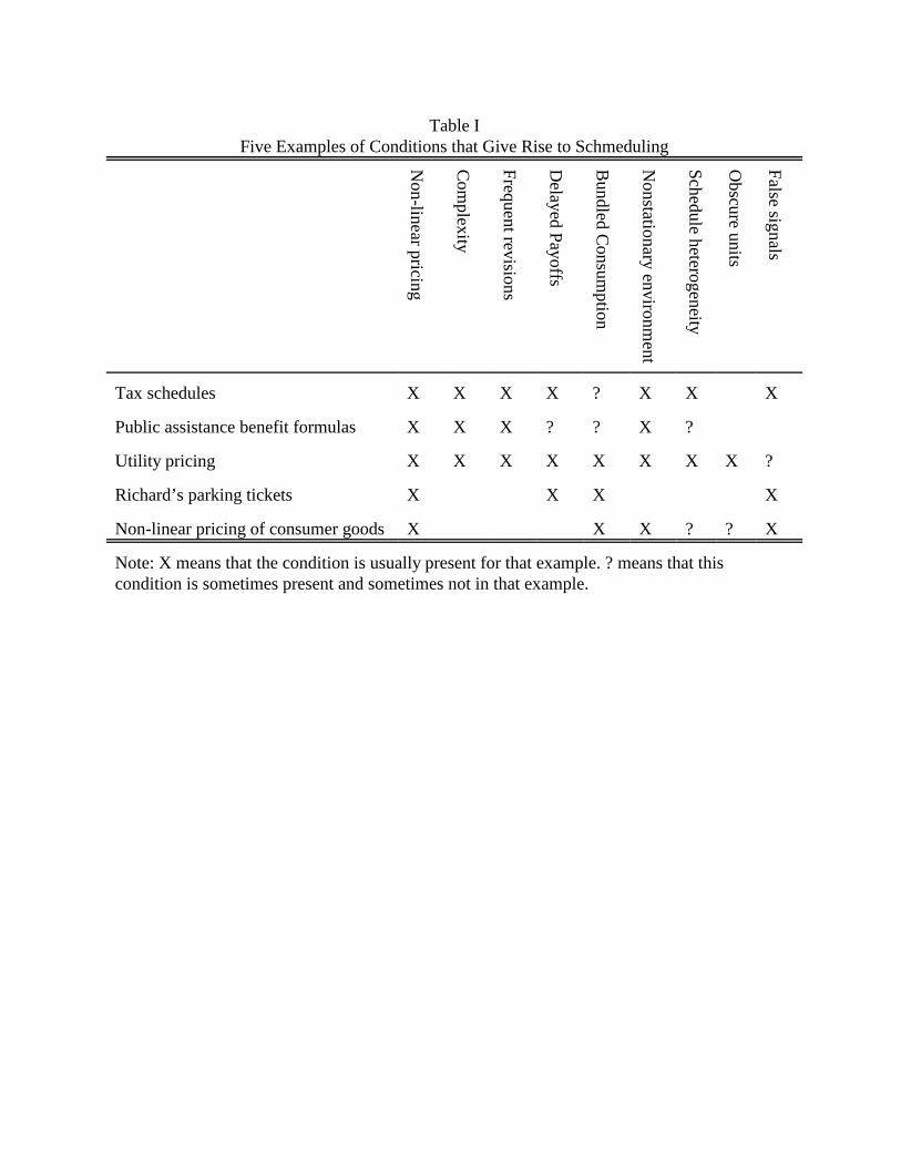
We now present five examples of areas of economic behavior in which we expect to

observe schmeduling. Table I shows which of the above conditions apply to each.

Tax Systems. A substantial body of research indicates that people do not understand their tax

schedules. Interviews with taxpayers in the UK (Brown, 1968; Lewis, 1978), Italy (Bises, 1990),

and Sweden (Brannas and Karlsson, 1996) and with EITC recipients in the U.S. (Liebman, 1996;

Olson and Davis, 1994; Romich and Weisner, 2002) all suggest substantial confusion about

marginal rates.2 Fujii and Hawley (1988) compare responses to a survey question about marginal

tax rates to calculated marginal tax rates using Survey of Consumer Finances data; they conclude

that there are significant differences.3 De Bartolome (1995) shows that people confuse average

4 Saez (2002) acknowledges the possibility of a behavioral explanation for the lack ofbunching.

5 The simulations in Saez (2002) suggest that uncertainty about what annual income willturn out to be is not large enough to explain the lack of bunching at kink points if elasticities areat least moderately large. Similarly, simulations of our own indicate that, in most cases, we candistinguish a rational consumer from a schmeduler unless income uncertainty is very great.

6 Dynamic tax considerations – such as tax rates on earnings converted to futureconsumption, tax rates on human capital investment, and the relationship between current workand future social security benefits – add additional complexity (Auerbach and Kotlikoff 1985;Kotlikoff, 1996).


and marginal tax rates when asked to make calculations using a tax table similar to those

published by the Internal Revenue Service with the 1040 tax form.

In addition, individuals’ actual choices often reveal traces of schmeduling. For example,

the evidence that taxpayers generally do not bunch at kink points (Heckman, 1983; Liebman,

1998; Saez 2002) and that people locate at places on the budget constraint where theory says that

they should not reside (Macurdy et al 1991) is usually interpreted as suggesting that taxable

income elasticities are small (Saez 2002) or that the specification of preferences in the analysis is

wrong (Heim and Meyer 2002).4 Schmeduling offers a different explanation. Lack of bunching

at concave kink points and the presence of people at convex kink points may arise because

people do not know or misperceive the tax schedule.5

More generally, the complexity of the tax code, with seven statutory marginal rates and

twenty-two provisions that “give rise to deviations between effective marginal tax rates and

statutory marginal tax rates” make it unlikely that most taxpayers calculate their marginal rates

accurately (Barthold et al, 1998). Other tax and transfer programs – state income taxes, food

stamps, student loans, housing assistance, etc.– make the task considerably more difficult.6

7 The summary statistics automatically produced by TurboTax when the taxpayer hasfinished filling out a tax return include the taxpayer’s average tax rate, but not the marginal taxrate. One must redo the tax return with an alternative income level to learn one’s marginal taxrate from this software.

8 Even if work effort stays constant, changes in marital status, family composition,housing consumption, life-cycle earnings patterns, and tax laws mean that people will often be ondifferent segments of the budget constraint.


Given the challenge of calculating marginal rates directly, it is worth considering what

alternatives people might employ, short of looking up the tax tables. In theory, they could infer

their true net wages by looking at their pay stubs to see how their after-tax income changes from

year to year in response to changes in effort, even without referring to tax tables or trying

hypotheticals in TurboTax.7 Such first-differencing calculations seem unlikely, particularly

given rapid changes in economic environments.8

Table I shows that the tax system features most of the conditions we predict should foster

schmeduling. Tax systems are complex, involve nonlinearities, and are revised frequently. The

payoff from a decision this January may not be realized until April of the following year. Often

very different decisions (labor effort of two people, sale of capital assets, degree of tax avoidance

undertaken) together determine a single annual payoff. Individuals are likely to be on a very

different point on the schedule than their friends or neighbors (and also hesitant to discuss their

incomes). Finally, taxpayers receive pay stubs that may lead them to conclude their marginal tax

9 The withholding schedule does not account accurately for non-wage income, and thegap between gross and net pay that the taxpayer observes on his paystub often reflects non-taxpayroll deductions for life insurance, dependent care accounts, medical savings accounts,parking, and the like. Thus, taxpayers may react to a number that is neither their marginal northeir average tax rate.

10 Confusion between average and marginal prices has been offered as an explanation forthe flypaper effect (that federal grants to state and local government significantly increase stateand local spending) by Courant, Gramlich, and Rubinfield (1979) and Oates (1979). Hines andThaler (1995) discuss this and other explanations for the flypaper effect.

11 In theory, welfare case workers could explain to their clients what the financial benefitfrom earning more would be. Evidence from a study of the California GAIN program suggests,however, that even when caseworkers were explicitly urged to discuss the returns to work withclients, they rarely did so (Meyers, Glaser, and MacDonald, 1998).


rate is merely 1-(net pay/gross pay).9 10

Welfare Programs. To our knowledge, income transfer systems create the most complex

schedules widely faced by ordinary citizens. Many recipients receive benefits from multiple

programs, each with its own schedule of how benefits fall (and occasionally rise) with increased

earnings. Even when the benefit-reduction schedule from a single program is linear, the

combined schedule will be highly nonlinear. Moreover, each program has complicated rules

about amounts of income that are disregarded before the benefit-reduction schedule is applied.

For example, in 2000 the food stamp program disregarded the first $134 dollars of income plus

20 percent of earnings (among a long list of other deductions) in a month. Thus, the way in

which earnings are allocated across months also affects benefit payments.11

Even economists have a hard time computing effective marginal tax rates for welfare

recipients. The complexity of the rules about what income is disregarded largely explains the

wide range of estimates of effective tax rates for AFDC recipients in the empirical literature –

12The schedule for the Earned Income Tax Credit (EITC) is particularly complicated. Thecredit initially increases with earnings, is constant at its maximum value for a range of earnings,and then is phased out as earnings rise even further. Since payment is usually made as part of anannual tax refund check, the EITC component of the refund is hard to determine. Empiricalresearch on the EITC has found that single mothers respond strongly to EITC incentives indeciding whether to work, but not in choosing how many hours to work (Eissa and Liebman,1996; Meyer and Rosenbaum, 2001; Meyer, 2002). Liebman (1998) attributes this combinationof results to the greater ease with which recipients can perceive the impact of the credit on theaverage return to work than on the marginal return.

13 Time limits make the welfare recipient’s decision problem into a complex dynamicprogramming problem of how to consume from a fixed potential-benefit stream. See Groggerand Michalopoulos (1999) on welfare time limits and Pollack and Zeckhauser (1996) on themore general problem of how to consume out of a fixed budget over multiple periods. Eachpaper finds that complex, nonintuitive strategies are optimal.


ranging from the work of Dickert, Houser, and Scholz (1994) who find cumulative rates of 15 to

40 percent, to the work of Giannarelli and Steuerle (1995) who find rates of 75 percent or more.12

Both program rules and unstable economic environments make it hard for welfare

recipients to know where they are on the schedule. Benefit reduction rates often vary based upon

the length of time a person has been receiving benefits,13 and recipients often experience large

discrete jumps in earnings levels; so knowing the marginal rate on one additional dollar of

income may be a very bad estimate of the payoff to the change (say from part-time to full-time

work) that the person is actually contemplating.

Some features of welfare programs make their incentives easier to perceive than those of

the tax system. Their accounting period is usually one month, rather than one year, enabling a

person to see an earnings change swiftly reflected in welfare benefits. Kling, Liebman, and Katz

(2001) report that a large share of recipients of housing assistance know that their rent will go up

by exactly 30 percent of any increase in their earnings, perhaps because of the monthly

accounting period; whereas, EITC recipients, with an annual accounting period, generally have

14In most cases, a public housing resident’s neighbor or cousin in another city canaccurately tell him or her what the effective tax rate is from housing assistance. A similar abilityto learn about schedules from acquaintances may explain the clustering of elderly workers withearnings just below the threshold for the Social Security earnings test (Burtless and Moffitt,1984;Friedberg, 2000). Gruber and Orszag (1999) show, however, that the amount of such bunchingthat occurs is quite small – at most 4.1 percent of the working population of 62- to 69-year-oldslocate just below the earnings-test threshold.


no concept of the EITC phaseout. A second possible explanation is that the 30 percent housing

tax rate has been constant for many years, and applies nationwide to everyone in public

housing.14 Other tax or transfer programs, by contrast, place individuals at different points and

slopes on the schedule, and rates vary across locales. Overall, public assistance provides

examples of most of the conditions listed in Table 1.

Utility Pricing. Utility pricing schedules, though simpler than tax and transfer schedules, still

have multi-tiered, nonlinear pricing. They have four additional features that make it difficult for

consumers to perceive the marginal price of consuming additional water, electricity, or heating

fuel. First, pricing schedules are sometimes not published on the monthly bill. Second,

consumers are often located at very different points on the schedule in different seasons – say,

demanding more natural gas in the winter. Third, pricing schedules often vary from season to

season – utilities charge more for natural gas in winter. Fourth, and most importantly, the link

between a consumer’s choices (how long to stay in the shower, whether to run a half-full

dishwasher, where to set the thermostat) and consumption is hard to observe. How many gallons

of water are used per shower, and how much does it cost to heat that water? Bills are presented

in consumption units that are not directly observable (and, like therms and kilowatts, are often

incomprehensible) to the consumer, and monthly payments aggregate hundreds of disparate

15 There is some empirical support for the proposition that utility consumers engage inschmeduling. Friedman (2002) finds that the consumption behavior of natural gas consumers isbetter explained by a model in which consumers respond to the total bill rather than a model inwhich they respond to marginal cost.

16 The roommate, who was not studying economics, did not counter with the argumentthat the owner would be excessively careless, not internalizing costs incurred by the roommate.


individual decisions (e.g., turning on the light and running the dishwasher). Such factors – a

nonstationary economic environment, delayed payoff, and bundled consumption (see Table I) –

combine to make it almost impossible to determine one’s marginal price by observing how bills

vary with behavior. How then do people make their decisions relating to utility use?15

Nonlinear Penalties, Fines, and Insurance Contracts. In 1959, one of us (RJZ) let his roommate

borrow his car early in the fall semester. His roommate returned the car, and mentioned that he

had received a ticket, but that it was free. Indeed, the schedule allowed two free tickets, then $5

for the 3rd, $10 for the fourth, and $20 for any ticket thereafter. The roommate asserted he owed

nothing. RJZ, believing that he would probably get four or five tickets in the year, suggested that

$15 might be his expected marginal cost due to the ticket, and that they could always settle up

when the cost became known at the end of the year.16

This sort of penalty structure is common. For example, automobile insurance rates often

start rising after a person has received more than 3 points on his license from moving violations,

or has made a certain number of claims under his comprehensive insurance policy. Criminal

sentencing guidelines often impose higher prison sentences on convicts who have previous

convictions, “three-strikes” laws being a draconian example. Medical flexible spending accounts

have zero out-of-pocket costs for initial units of consumption; consumers pay the full price once

17In some cases, merchants may hurt themselves by presenting pricing in a way thatproduces schmeduling behavior. Shutterfly.com describes its holiday cards as costing 82 centsper card if 100 are purchased and 69 cents per card if 200 are purchased. Thus the marginal costof the second 100 cards is only 56 cents per card. We suspect that most consumers decidingbetween 100 and 200 cards perceive the marginal price as 69 cents and that Shutterfly couldincrease both its sales and its customers’ consumer surplus by describing its pricing as a two-partschedule, so as to get some additional people to respond to the schedule rather than a schmedule.


the accounts are exhausted. In each of these cases the true marginal cost of additional

consumption early in the time period depends on expected consumption later in the time period

and can be far above the immediate cost. We conjecture that confusion often arises when the

within-accounting-period payoffs present false signals of the ultimate marginal price.

Nonlinear Pricing of Consumer Goods. For most consumer goods, such as milk or clothing,

consumers are told the price at the time of contemplated purchase, and the per-unit price does not

vary with quantity. However, even with ordinary goods, consumers are sometimes offered

quantity discounts. Such pricing may lead consumers to schmedule.

Typically, the schmeduler is hurt by failing to rationally optimize. Say he uses ironing.

He consumes units whose marginal cost exceed his marginal benefits if the schedule is convex,

and vice versa if the schedule is concave. This assumes that the schedule setter does not change

the schedule in response to the schmeduler’s behavior. As we discuss further below, if the

schedule setter does respond, that can help or hurt the schmeduler, depending on the schedule

setter’s goal, the shape of the schedule, and the particular schmeduling behavior.17

Sophisticated businesses may capitalize on the confusion that pricing schedules create,

causing some customers to pay more or purchase more than they otherwise would for the service.

Cell phone packages with prices that rise steeply if a customer uses more than his or her allocated

18 Cell phone companies may be counting on people to consume more than they plan, andto pay high rates on extra minutes, or – like auto rental companies offering cheap full tanks –may be trying to get customers to purchase more minutes to protect against exceeding the limit. This process is complicated because cell phone companies compete fiercely, and presumablythere is adverse selection – frequent callers choose flat-rate plans, for example, with schmedulingtempering adverse selection.

19 In other words, consumers may infer marginal prices by calculating the change inpayoff divided by the change in quantity consumed over subsequent accounting periods. Alternatively, they may infer marginal prices by comparing their own situation to that of a similarperson who made a slightly different choice.

20 A third, more extreme, form of schmeduling is ostriching. This occurs when people areso overwhelmed by the complexity of schedules that they ignore the schedule altogether. Examples of this include: 1) people ignoring the marginal social security benefits they receive inthe future from social security payroll tax payments; 2) consumers making choices based onfactors other than price when the pricing schedules are too complicated, as appears to occurfrequently with purchasers of medigap insurance policies – as evidenced by the wide range ofprices at which identical policies can be purchased; and 3) consumers purchasing mutual funds


amount of monthly minutes presumably fall in this category. It is next to impossible for a

customer to know how many minutes he or she has used up so far in the month. Moreover, as

the quotation at the top of the paper shows, there is no necessary connection between when the

customer makes the calls and which months the calls are assigned to for billing purposes.18

III. How People and Pigeons Respond to Schmedules

People who are fiercely rational or who face very simple pricing schemes may know

exactly where they are on their various schedules. Some may use first-differencing to estimate

marginal prices,19 and other quasi-rational methods may be near optimal. Some affluent people

hire people to do the calculating and optimizing for them.

Our proposition, however, is that people facing pricing schedules often engage in two

prominent variants of schmeduling: ironing and spotlighting.20 Evidence from experimental

with 100 basis point annual fees, even though information of the fees is readily available. We donot discuss ostriching further in this paper because we think it will be very difficult to develop ageneral theory capable of predicting how consumers will behave in these circumstances.

21 In fact, in the home heating example we doubt that people ever do the conversion toprice per therm. Nonetheless, in thinking about marginal consumption decisions, we believepeople make those decisions by thinking of increments to the $300 monthly bill which, since itincludes the price of inframarginal consumption, will result in behavior that is responsive toaverage rather than marginal prices.

22 Keeler and Rolph (1988) show, using data from the Rand Health Experiment, thatconsumers who have nearly exhausted health insurance deductibles spend no more on healthcarethan consumers who are far from exhausting their deductibles. However, consumers who havecompletely exhausted the deductibles do consume more in response to the lower price. Thisfinding -- that people respond to their local price and fail to incorporate expected futureconsumption into their calculations – is consistent with spotlighting.


psychology – mostly with pigeons but some with humans – establishes ironing and spotlighting

as plausible models of how people behave when faced with complicated schedules. Moreover,

our theory makes predictions of when each type of behavior will be observed. Ironing occurs

when there is a single payoff for all of the bundled choices within an accounting period.

Spotlighting occurs when there are multiple within-accounting-period payoffs.

With ironing, people smooth over the entire range of the schedule. They perceive (or

treat) the average price as the marginal price. Thus one decides whether to lower the thermostat

by noting that $300 per month represents an average price of 60 cents per therm, rather than 89

cents for the last (and next) therm of natural gas.21 With spotlighting, people respond to the

instantaneous payoff in the current sub-period without considering effects for the remainder of

the accounting period. Thus users of medical flexible spending accounts may act as if

consumption in January is free (or near free), ignoring the fact that by the end of the year they

may well be paying the full cost of marginal care.22

23 Schmeduling also has antecedents in the behavioral economics literature. It is mostclosely related to the literature on calculation errors (Tversky and Kahneman, 1974), boundedrationality (Simon, 1978), and mental accounting (Thaler, 1985). The confusion betweenimmediate and end-of-period prices that is the essence of spotlighting is related to the literatureon time-inconsistent preferences and self-control (Thaler and Shefrin, 1981; Laibson, 1997;Bernheim and Rangel, 2002).


These same behaviors are well documented in the experimental psychology literature for

a wide range of species including pigeons, rats, monkeys, and humans. In particular,

schmeduling is closely related to Richard Herrnstein’s theories of melioration and distributed

choice.23 We summarize the experimental psychology evidence in appendix A.

Whether these theories can in fact explain people’s behavior in the applications that are

our focus remains to be seen. Before turning to empirical tests of these theories in section V, we

first discuss the potential welfare implications of such behavior.

IV. Welfare Implications of Ironing and Spotlighting

To illustrate how schmeduling affects welfare, we first consider simple schedules with

two linear segments, and a world with two types of responders. We start with ironing, and study

schmeduling in three contexts: a profit-maximizing monopolist, a Ramsey-pricing public utility,

and a social-welfare-maximizing tax authority. We also illustrate the deadweight loss that

arises from spotlighting. Then, for the tax authority case, we drop the simplifications, solve the

Mirrlees optimal tax model under ironing, and present empirical estimates of the welfare

implications of ironing for the U.S. tax system.

Ironing in Two-segment Two-type Models

24 Convex schedules will not be observed in situations where big users can easily make aseries of small purchases to reduce their cost. Convex schedules are quite common with utilitypricing or taxes, where breakup would be hard or illegal. Insurance offers an interesting case inwhich it is often not possible to buy half as much from two sources since there are prohibitionsagainst insuring the same thing twice (or at least against collecting if you do). Hence, people buyall their insurance for a home through a single insurer who in turn can charge more the greaterthe percentage of your home’s value you insure. The same holds true for mortgages. An 80percent mortgage costs more than twice a 40 percent mortgage, but you can’t buy two separate 40percent mortgages that will behave like a single 80 percent mortgage. The Rothschild-Stiglitzinsurance results, and their push for nonlinear pricing, all hinge around these issues. With lifeinsurance, in contrast, you can buy two smaller policies that have the same impact as one largerpolicy, and prices tend to fall with the amount insured, due to negative correlations betweenincome and mortality risk and because of savings in transaction costs.


For simplicity, in the monopolist and Ramsey-pricing cases, we shall assume that goods

are produced at constant marginal cost and that there are no economies of scale on the

consumption side (such as in delivery). Throughout, we focus on situations where the optimal

schedule from the standpoint of the schedule setter is convex: prices rise with quantities

consumed, and tax rates rise with income. This “rising-price” case is most relevant to the tax-

and transfer- policy applications we turn to later in the paper. Convexity could arise to maximize

profits in the monopolist case or to maximize efficiency in the Ramsey-pricing case, if the high

demander has lower elasticity. Or it could be imposed to meet distributional concerns in the tax

example, whatever elasticities might be.24 There are, of course, situations where optimal

schedules are concave, for example when there are economies of scale in production, or where

large users have more elastic demand (for example, if they have lower per-unit transaction costs

for switching suppliers).

Ironing: The Profit-Maximizing Monopolist. The monopolist sets a price schedule where the

first k units cost p1 each, and all subsequent units cost p2, where convexity requires that p2 > p1.

25 In this figure we assume that they have the same income because this allows us todepict them as facing the same budget constraint, but our results do not require them to have thesame income.


Given ironing, and but two types of responders, call them HI and LO, two-segment schedules can

reproduce the results of significantly more complex schedules. Figures 2a and 2b illustrate the

consumers’ and profit-maximizer’s decision problems. The two consumers have equal incomes,

but differ in their tastes for the good.25 At any point, consumer HI is willing to give up more of

the other good to get another unit of the monopolist’s good; i,e., he has less elastic demand.

As depicted in Figure 2a, for rational responders, the monopolist selects three parameters:

p1, p2, and a kink point where the price switches. The choices are such that LO consumes at the

kink (point A representing K units), and HI chooses some point on the p2 segment of the budget

constraint. (His indifference curve is tangent in this rational case.) In maximizing its profits, the

monopolist faces several constraints that apply whether the consumers are rational or

schmedulers. First, he is restricted by assumption to a pricing schedule that starts at zero and that

rises with quantity consumed. Second, he must offer a segmented linear schedule, rather than

two points. Third, both responders must prefer their choices to zero consumption. Fourth, there

is a no-envy condition. HI must prefer some choice on the p2 segment to point A. Finally,

observe that in optimizing against LO, the monopolist has two different policy tools, the price

and the length of the pricing segment. However, it turns out that it is never optimal to prevent

LO from consuming as much as he wants at p1, as we explain in conjunction with Figure 2b.

Figure 2b shows the solution to the monopolist’s profit maximization problem when

confronted with rational consumers and then with schmedulers. The vertical axis measures net

revenue; that is, marginal cost is subtracted. We first consider the solution when consumers are

26 To see this, consider interior point T as a possible kink. The monopolist would securemore from LO by offering the alternative p1 that runs to R, the point vertically above T on thefrontier. This is also the point that LO would choose at this new p1. The monopolist also getsmore from HI. Say that the best the monopolist can do against HI given a kink at T is V. With akink instead at R, he will have a lower marginal price for any quantity-net revenue pair northeastof R. Hence he could receive greater net revenues from HI, e.g., at E.


rational. Look at the outcome for LO, and the Feasibility Rational LO curve. This shows how

profits to the monopolist from sales to LO vary with p1 (the slope of a line from the origin to the

curve). At the right-most end, p1 is low, quantity demanded is high, but revenues just cover

costs. As we move left on the curve, p1 is rising. LO will always consume on this feasibility

frontier. In other words, the kink point – R in the figure – will always occur at the point that LO

would choose if offered the opportunity to consume an unlimited quantity at a price of p1 per

unit.26

Point S indicates the point where net revenue is maximized, taking into account only the

sales to LO. The slope of the curve from the origin through S is p1s. Posit that the optimal

outcome is to have LO consume at R and HI at E. The monopolist will set p1>p1s (along

Feasibility Rational LO) – a level that is higher than would be optimal were he optimizing

against the low type in isolation. Doing so allows him to lower p2, thereby increasing the

quantity consumed by and profits from HI. Raising the price on inframarginal units and lowering

them on marginal ones is not unlike imposing a fixed cost on HI and then a lower per-unit price,

thereby yielding higher profits from HI. But this comes at the cost of lower profits from LO.

Point R represents the optimal balancing of profits from HI and profits from LO. It will therefore

always be to the left of S, the maximum on the Feasibility Rational LO curve. This higher p1

results in lower utility for LO than if the monopolist were optimizing against LO in isolation.


Now consider the curve labeled “Feasibility Rational HI.” This curve, added from point

R, shows how varying p2 affects profits to the monopolist from sales to HI. Convexity requires

that p2>p1. Therefore the curve ends at point D, the level of consumption chosen by HI if the

slope of the second segment just equals the slope of the first. When p2 becomes sufficiently high

-- steeper than the “Feasibility Rational HI” curve at point R – HI prefers the kink point to any

point on the p2 portion of the schedule and consumes at point R. Point E indicates the HI type

consumer’s consumption at the level of p2* , the value that maximizes the monopolist’s profits.

When consumers are ironing, the profit maximizer’s problem takes on a different cast.

The LO consumer is unaffected, since he merely responds to a single price, which is both average

and marginal. HI, however, responds to his average price, not p2. Hence, his feasibility curve

assumes that a price line pivots starting at the origin. His feasibility frontier lies strictly above

that for rational HI to the northwest of D (at D the average price and marginal price are equal).

That is because he perceives a lower price at the margin for any amount of revenue raised. Thus,

for example, if the HI ironer were offered the price schedule through R, with p2* beyond, he

would consume at a point like G, with greater consumption than at E.

Given that HI is responding as an ironer, the location of the first segment of the schedule

does not matter. Thus, it is optimal to move the first segment to S, with a caveat about envy,

discussed below. HI will be offered the schedule running from S through F. He consumes at F

where his indifference curve is tangent to the price line from the origin through F. The envy

caveat applies if HI prefers S to F. The point Se on the Feasibility Ironing HI curve shows the

point where HI is indifferent to S. In this case, F is preferred to S. If it were not, it would be

optimal to move S to the left and F to the right until envy was just eliminated.

27 In contrast, we will see that in the Ramsey pricing and optimal income tax models, theschedule setter cares about social welfare and will therefore need to know the preferencesunderlying the behavior he observes. He may draw erroneous inferences about preferences if hedoes not realize that consumers are ironing.

28 Today, most utilities have such schedules for several purposes: to limit demand sincenew capacity costs more than old, to control environmental externalities, and to achievedistributional objectives since big users tend to be richer.


It is readily seen that the monopolist is better off with ironing behavior. He could always

offer the optimal rational schedule. Under that schedule, an ironing HI would operate at point G,

which offers more net revenue than E, the point produced by the rational HI. Since the

monopolist also selects S rather than R as the kink point, LO is definitely better off with ironing.

HI, however, is likely to be worse off as an ironer, since at a point like F he pays more and

consumes less than at E.

We have posited that the schedule setter is a shrewd maximizer who understands his

consumers’ psychological propensities. But this is not necessary. He can merely vary the two-

part price schedule through trial and error, and will reach the same outcome as would an

optimizing schedule setter.27

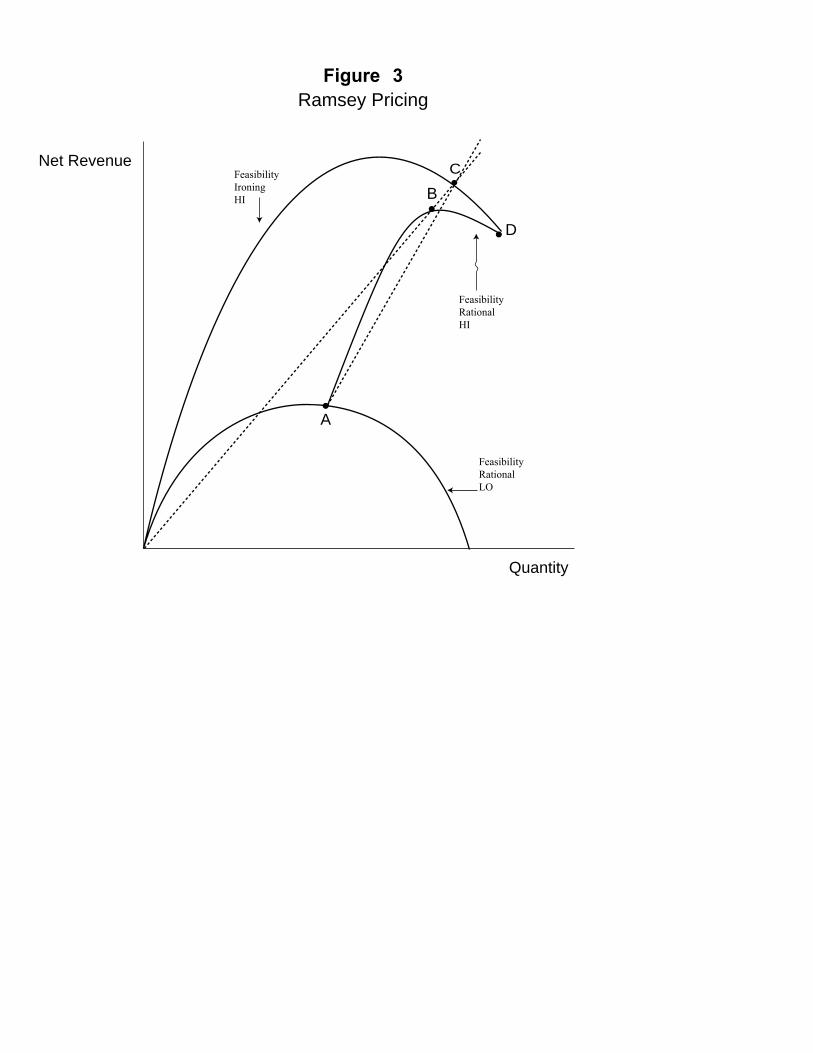
Ironing: A Ramsey-Pricing Utility. The Ramsey pricing model bears important similarities to the

monopolist case, though the objective functions differ. Whereas the monopolist maximizes

profits, a Ramsey pricer minimizes deadweight loss, subject to the constraint that profits cover

fixed costs. We continue to assume a convex schedule, where the higher-volume user pays a

higher per-unit charge on marginal units.28


Figure 3 shows the Ramsey pricer’s solution. The feasibility constraints in the rational

case for both consumers are identical to those in the profit maximizing example since the only

thing that has changed is the producer’s objective. Let points A and B represent the optima,

assuming that LO and HI are rational and that HI does not envy LO. In other words, these points

reflect the inverse elasticity rule. Note that point A lies to the right of the revenue maximizing

point because the Ramsey pricer is trying to maximize social welfare, not revenues, and therefore

takes LO’s utility into account.

If HI is an ironer, it is easy to see that the Ramsey pricer can do better. He simply offers a

schedule with the second segment going from A to C, where C lies on the line from the origin

through B. HI will consume at C. HI is better off, since points strictly better than B – those in

the triangle formed by extending horizontal and vertical lines from B to the line connecting A

and C – were available to him. In this solution, there is no envy, since UH(C)> UH(B)>UH(A).

Moreover, revenues are higher, implying that some could be given back to LO, HI, or both. This

merely shows how to beat the rational outcome – in other words that a Pareto improvement

exists. By adjusting the locations of A and C, the schedule setter with ironing can further reduce

deadweight loss, while making sure not to adjust so far that HI prefers A to C.

Ironing: The Optimal Income Tax. We assume that the tax schedule is convex: i.e., that marginal

tax rates increase somewhere and decrease nowhere. The presumed justification is not

differential elasticities, but distributional concerns, i.e., a presumed declining marginal utility of

money. Our analysis has both taxpayers pay positive amounts, though allowing for net negative

taxes would merely involve rescaling the axes. Figure 4 shows our analysis. The scales on the

29 Note that the marginal tax rate for the second, higher, bracket will be below therevenue- maximizing one, since HI’s welfare counts somewhat and the loss in revenue frommoving away from the revenue-maximizing point is initially zero.

30 Though we have shown that ironing behavior allows for a Pareto-superior outcome, theoptimal outcome given ironing may not be Pareto superior. For example, if ironing gets rid ofmost of the deadweight loss associated with taxing HI, the optimal scheme may cut his welfarewhile substantially raising welfare for LO.


two axes are drawn so that post-tax income equals pre-tax income (the usual 45 degree line)

along the steep dotted line ending at F. This makes the diagram easier to read. Assume that the

tax schedule depicted with the solid lines is the optimal schedule if the two taxpayers are

rational. Thus the L type taxpayer chooses point A and the H type taxpayer chooses point B.29 A

superior outcome is vailable if HI is a schmeduler. We draw a straight line from the origin

through point B to find a point, C, on this line that is on the schmeduler’s feasibility curve (in

other words, the schmeduler’s indifference curve is tangent to the average tax rate line at this

point), and that provides higher utility than at B. In particular, the schedule setter can get HI to

choose this point, by offering a tax schedule with the same tax rate through point A as in the

rational case and then setting the second tax rate so that the tax schedule beginning at A goes

through point C (the lightly dotted line). With this new schedule, the schmeduler not only has

higher utility, but also generates more tax revenue (he has higher pre-tax income and is paying

the same average tax rate as at B). Given a sophisticated schedule setter, the tax scheme with

schmeduling is Pareto superior to the one without.30

General statements about progressivity given schmedulers, as opposed to rational

responders, are not possible. The answer depends on the progressivity measure employed. We

are confident of one result. In comparison with the optimal tax scheme with rational responses,

31 The arguments regarding no-envy conditions and naive schedule setters in the optimalincome tax case follow directly from those in the previous two models.

32 See de Bartolome (1995) for an earlier statement of this result.


there exists a Pareto-superior scheme given schmeduling that simultaneously collects more taxes

from HI, has a higher average tax rate imposed on HI, and leaves HI better off. This is achieved

at a point slightly below C on HI’s feasibility frontier. HI is still better off than he was at B, but

pays more in taxes and has a higher average tax rate.31

One other point merits emphasis. Given any tax schedule, an individual is better off if he

is rational. This can be seen most clearly by observing that the ironer who is tangent to the

average tax rate curve at C would achieve higher utility by moving to the left along the second

segment of the tax schedule. Ironing yields its benefits because it makes respondents less

responsive to marginal rates. Given that, the schedule setter offers a more favorable tax

schedule.32 The best situation for a taxpayer is to be rational while everyone else an ironer.

The results from our geometric presentations are straightforward. Ironing behavior

eliminates some of the deadweight loss from high marginal prices or taxes. This implies that

when the optimal rational schedule is convex, superior outcomes are available for the

monopolist, for the Ramsey pricer, and for the setter of an optimal income tax. In the latter two

public finance contexts, outcomes that are Pareto superior to the rational-responders’ outcome

are available, though such an outcome will not necessarily be chosen by the sophisticated

schedule setter.

Spotlighting. We turn now to the welfare implications of spotlighting. We continue to analyze

a convex schedule (p2>p1) with two linear segments, but here only one consumer is required. We

33 It is possible to come up with examples in which schmedule-setting opportunitiesanalogous to those under ironing would be available given spotlighting responders. For example,if a tax authority were to withhold at different rates throughout the year, depending on where thetaxpayer then was on the annual tax schedule – as opposed to the actual practice of withholdingbased on expected annual earnings – this would create opportunities for schmedule setting thatwould be quite similar to those in the optimal taxation example we analyzed under ironing.


present a graphical analysis of a model with two discrete sub-periods. Appendix A contains an

algebraic analysis of a continuous-time model. For simplicity, we assume no discounting. We

focus on the magnitude of the deadweight loss that occurs when the consumer misperceives or

miscomputes prices. This contrasts with our ironing analysis, where we assumed that

sophisticated schedule setters reoptimized to take account of consumers’ schmeduling. Schedule

setting is generally less interesting in the spotlighting context than with ironing. From the

seller’s standpoint, spotlighting behavior simply amplifies the demand curve in the initial price

range.33

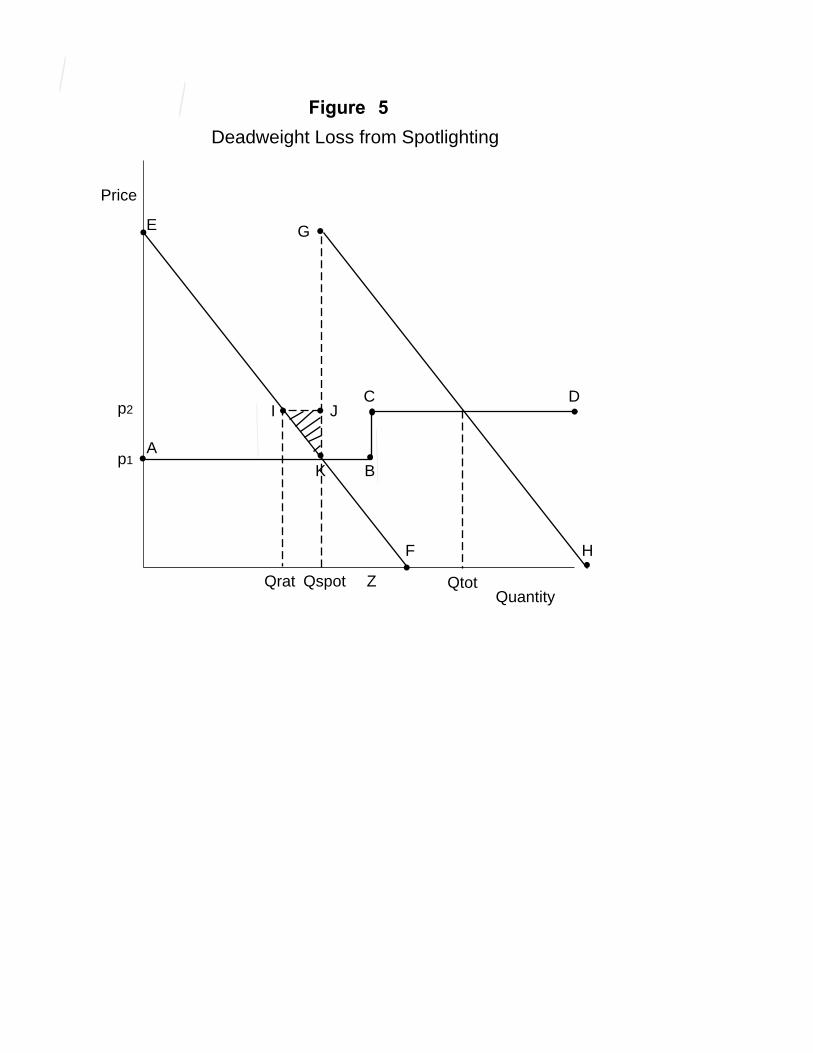
Figure 5 illustrates the deadweight loss that arises from spotlighting when a price

schedule has two segments. The consumer pays p1 for the first Z units, and then pays p2 for

subsequent units. This schedule is shown as segments AB and CD on the diagram. The

consumer chooses consumption in each sub-period. (A sub-period could be a day, with the price

schedule applying to aggregate consumption during a monthly accounting period.) Consider two

sub-periods. The consumer’s demand curve for the first is EF. Since the consumer is a

spotlighter, he responds only to the local price and ignores the impact of this decision on the

price(s) he will face in the second sub-period. Therefore, first sub-period consumption is

determined by the intersection of the segments AB and EF, and he consumes Qspot of the good.

The demand curve for the second sub-period, GH, begins at Qspot because there is a single (two-


part) price schedule for the entire accounting period. Total consumption for the two sub-periods,

Qtot, is determined by the intersection of GH and CD.

Spotlighting leads to overconsumption because the consumer ignores the true opportunity

cost of his first-sub-period purchases; he behaves as if he is foregoing p1 of other goods for each

unit consumed, whereas the true cost is p2. The amount of overconsumption is Qspot-Qrat; the

deadweight loss from this overconsumption is the triangle IJK.

Empirical Magnitude of Welfare Effects Are the welfare effects of schmeduling large enough to

be of policy interest? While the answer will depend on the specific application, there is one

important case – the federal income tax in the presence of ironing – where the data and

methodology are readily available to assess the magnitude of the welfare effects. We first

examine the welfare effects under the 2000 U.S. tax code. Then we solve the Mirrlees optimal

tax problem under ironing, and show how the structure of the optimal tax schedule under ironing

differs from that under the standard model.

With a convex tax schedule, ironers will perceive a tax rate that is lower than the true

marginal tax rate. Hence, they will earn more income (work harder), and the tax system will

impose a smaller deadweight loss. To assess the quantitative importance of this effect, we

conduct simulations using the 1998 IRS public use sample of tax returns and NBER’s internet

Taxsim model. We “age” the sample to reflect 2000 income levels and use tax schedules for that

34 2000 was the most recent year covered by Taxsim at the time we did these calculations. We dropped a couple dozen observations from the sample for whom Taxsim calculated marginaltax rates below -40 percent or above 50 percent.


DWL TY=−

12 1

2

ετ

τ, (1)

year.34 Following Feldstein (1999), we calculate deadweight loss using the Harberger-Browning

approximation as

where TY is taxable income, , is the elasticity of taxable income with respect to the after-tax

share, and J is the tax rate. We use a value of 0.4 for ,, based on the estimates of Gruber and

Saez (2002). Since deadweight loss is linear in ,, readers can readily employ alternative values.

We assume that taxpayers are ironers: they mistake their average tax rates for their

marginal tax rates. Then we ask what would happen if we informed these taxpayers of their true

marginal rates. It is worth emphasizing that an ironer optimizes at a point where his indifference

curve is tangent to the average-tax line (a line from the origin) and that is simultaneously on the

frontier of the tax schedule. Point C in figure 4 represents such a point (for the tax schedule

whose second segment extends from point A through point C). For a given convex tax schedule

and standard preferences, this is a unique point for each individual. The Harberger-Browning

approximation applies to our thought experiment because the deadweight loss effect of informing

an ironer of his true marginal rate is identical to that for a rational consumer who experienced an

actual change in tax schedule from the average tax line perceived by the ironer to the true tax

schedule.

35 For comparability with the main results in Feldstein (1999) these results ignore thepayroll tax. Treating the personal income tax as an increment on top of the payroll tax wouldproduce larger deadweight loss estimates.

36 Our estimates for the rational case are quite similar to Feldstein’s (1999) estimates. Feldstein, using an elasticity of 1.04, estimates that DWL from the personal income tax in 1994was 32.2 percent of revenue. Multiplying our DWL estimate by (1.04/0.4) produces an estimateof 30.9 percent. Interestingly, our estimate that DWL under schmeduling is 48 percent lowerthan under the rational case is very similar to that of de Bartholeme (1995) who does anillustrative calculation for a representative worker with mean earnings using parameter estimatesfrom Hausman (1981) and finds that DWL falls by 43 percent when taxpayers substitute averagerates for marginal rates.

37 With a taxable income elasticity at Feldstein’s preferred value of 1.04, the marginalexcess burden is $1.89 per dollar of revenue raised under the rational model and 52 cents underthe schmeduling model.

It is worth emphasizing that existing estimates of the elasticity of taxable income come


Table II presents our results. In the data, taxpayers have taxable income of $4.233 trillion

and pay income tax of $974.7 billion. Assuming ironing, the Harberger-Browning formula yields

deadweight loss of $56.7 billion, or 5.8 percent of revenue raised.35

We estimate that if taxpayers were informed of their true marginal tax rates, taxable

income would fall by about 5 percent to $4.020 trillion, and revenue would fall by about 6

percent. Deadweight loss would rise to $109 billion, or 11.9 percent of revenue raised.36 These

differences in income, revenue, and deadweight loss are all economically significant.

The marginal excess burden of taxation can be computed similarly. Consider a 10

percent increase in all marginal tax rates (for example, a 20 percent marginal tax rate would

become 22 percent). Under the schmeduling model, revenue increases by $82.5 billion and

deadweight loss increases by $13.9 billion for a marginal excess burden of 17 cents per $1 of

additional revenue. In the rational model, revenue increases by $68.9 billion and deadweight loss

increases by $27.2 billion, representing a marginal excess burden of 39 cents.37

from studies of behavioral responses to tax changes. These elasticities are calculated by dividingthe change in behavior by the change in after-tax share. The changes in after-tax shares in thesecalculations are based on marginal tax rates. Changes in after-tax shares calculated based onperceived tax rates (i.e., average tax rates) would be smaller, resulting in larger elasticitiesrelative to the perceived change in after-tax shares. Therefore, it might be appropriate to uselarger elasticities in the calculations above. This would produce higher estimates for thedeadweight loss. However, it would not alter the estimates of the relative amount of deadweightloss under schmeduling and the rational model (since we would simply be using higherelasticities in both calculations).

There is one piece of natural experiment evidence that is potentially inconsistent with thepredictions of our ironing model. Feldstein (1995), Eissa (1995), and Auten and Carroll (1997)provide evidence that high-income taxpayers increased their incomes substantially in response tothe reduction in marginal tax rates from the Tax Reform Act of 1986 (TRA86). Since TRA86was designed to be distributionally neutral, it affected average tax rates only slightly at mostincome levels. Thus, our ironing model would predict little behavioral response to this taxreform.

This evidence does not lead us to abandon our schmeduling model. First, we have arguedthat while many individuals schmedule, some individuals are rational. The very high-incometaxpayers studied in the TRA86 literature are likely to be among the most rational of alltaxpayers. Thus they are the ones whom we would least expect to observe engaging inschmeduling. Second, there is a large literature by Slemrod (1990), Goolsbee (2000), and otherssuggesting that the TRA86 evidence is a product of widening income inequality and the shiftingof income between the corporate and individual income tax bases, not of behavioral responses totaxation. If we are able to accumulate evidence demonstrating that taxpayers often engage inironing, this will increase the probability that these alternative interpretations of TRA86 arecorrect.


The Optimal Income Tax Under Ironing

The Mirrlees optimal income tax problem seeks to find the tax schedule that maximizes

social welfare subject to a government budget constraint and to an incentive compatibility

constraint for each worker, assuming that the government can observe workers’ earnings but not

their skill level. Recent papers by Diamond (1998) and Saez (2001) have significantly advanced

the optimal income tax literature by reformulating the problem in a way that makes transparent

the factors that determine the shape of the optimal tax schedule.

38 This is the formula assuming quasilinear preferences (implying equal compensated anduncompensated elasticities) and with the social marginal utility of someone with infinite incomeequaling zero.


( )T

Te

n

p G dF

pfn'

',

111

−=

+

×

− ′

−

∞

∫(2)

Diamond (1998) shows that with quasilinear preferences, the marginal tax rate, T’, at

each skill level, n, satisfies

where e is the labor supply elasticity, p is the multiplier on the government budget constraint

(equal the average over the population of the marginal social welfare), G(u) is social welfare for

an individual with utility, u, and f and F are the pdf and cdf of the skill distribution, respectively.

Saez (2001) shows that the upper tail of the income distribution for married couples in the U.S.

follows a pareto distribution with a pareto parameter of about 2 and that the asymptotic tax rate

(the tax rate on taxpayers with very high incomes) from the optimal tax problem is therefore

where e is the labor supply elasticity and a is the pareto parameter.38 Thus with a pareto11+ea

parameter of 2 and a taxable income elasticity of 0.5, the optimal asymptotic tax rate would be

0.5.

In appendix C, we derive analogous results under ironing. The main difference from the

standard problem involves replacing the first order condition for individual maximization

of with the ironing first order condition . The former (maximizing)( )v n T' '= −1 ( )v n Tny' = −1

equates the marginal disutility of effort and the marginal return to an extra hour of work, whereas

39 We follow Diamond’s notation in which y is labor supply measured as a percentage ofthe maximum possible labor supply, and v(1-y) is the disutility of effort.

40 We thank Emmanuel Saez who found an error in our original derivation of the Mirrleesfirst order condition under ironing and showed us that the first order condition has the form givenhere. This first order condition turns out to be identical to the first order condition for thecontinuous case of Saez’s (2000) model of the extensive margin of labor supply, a coincidencethat can be attributed to the fact that labor force participation decisions (holding hours fixed)depend on average tax rates just as the intensive margin decisions of ironers do. We also thankErzo Luttmer for extensive coaching on the Mirrlees problem.

41Appendix C describes the simulations in further detail.


the latter (ironing) equates the marginal disutility of effort and the average return to work.39 The

resulting first order condition for the Mirrlees problem given ironing – analogous to the Diamond

result given in equation 2 above – shows how the average tax rate at a given skill level relates to

both the labor supply elasticity and to the ratio of marginal social welfare at the skill level to the

multiplier on the government’s budget constraint:40

The asymptotic marginal (and average) tax rate in the ironing model is . Thus with an1

1e +elasticity of .5 and a pareto parameter of 2, the optimal rate on high income taxpayers is .67

under ironing compared with 0.50 under the standard model.

Figure 7a shows simulations of the optimal average tax rates implied by this first order

condition for three different elasticities. To be comparable with Saez (2001), the simulations use

a skill distribution taken from the 1992 earnings distribution of married U.S. taxpayers and

assume a quasilinear utility function and a logarithmic social welfare function.41 The optimal tax

T nynyT ny

nye

G up

( )

( )( )

.1

11

−= −

′

(3)


schedule under ironing has two interesting features. First, average tax rates at the bottom are

negative. In this model it turns out to be optimal to have a fairly large EITC-like program, even

without the extensive-margin considerations that underlie similar conclusions by Liebman (2001)

and Saez (2002). The intuition behind this result is that the negative effects of the EITC phase-

out in a standard model do not arise in a model in which people are responding to average tax

rates – even as the EITC is being phased-out, average tax rates are negative. Second, average tax

rates quickly become very high. Once earnings reach $50,000, average tax rates are already at 40

percent.

Figure 7b plots the optimal marginal tax rates under the standard Mirrlees model and the

ironing version of the Mirrlees model. The results for the standard model use an elasticity of 0.5

and are indistinguishable from those with the same elasticity presented in Saez (2001) . We

present results using the ironing model for two different elasticities: 0.5 and 0.8. These two

ironing results allow us to conduct two different comparisons. The first comparison – using both

results with the 0.5 elasticity – assumes identical preferences for ironers and for rational

taxpayers and shows how the optimal tax schedule differs under the two assumptions about how

people perceive incentives. The second comparison - using the 0.5 elasticity for the standard

model and the 0.8 elasticity for ironing – crudely adjusts for the fact that empirical estimates of

taxable income elasticities would generally be higher if they had been calculated under the

assumption that people were ironers. Since changes in tax schedules typically result in larger

changes in marginal tax rates than in average tax rates, a given change in behavior implies a

larger elasticity if people are responding to average tax rates. Thus to be consistent with

behavior observed in the past requires an elasticity of 0.5 if people are rational but a higher

42 The credit was partially refundable for some taxpayers with three or more children.


elasticity if people are ironers. The figure shows that the marginal tax rate approaches the

asymptotic rate much more quickly under ironing than under the standard model.

Our overall assessment from these two tax examples is that schmeduling behavior can

make a major difference. When schmedulers face a convex schedule, their nonrational behavior

increases efficiency. Were the schedule concave, the opposite result would apply. We have

proceeded inductively thus far: assume a behavior and distill the consequences. The remainder

of our paper is deductive. It presents two empirical studies that test for the presence of

schmeduling behavior.

IV. Empirical Tests

This section conducts two empirical tests of schmeduling. The first uses data from before

and after the 1998 introduction of the child tax credit to test for ironing. The second uses data

from the San Diego food stamp cash out experiment to test for spotlighting. In addition to

providing empirical evidence on whether schmeduling is occurring in these two instances, these

examples illustrate the kinds of conflicting predictions that can allow one to distinguish between

the rational and schmeduling models more generally.

A. 1998 Introduction of the Child Credit

Beginning in 1998, U.S. taxpayers with children could claim a $500 per child tax credit.

In most cases, this credit was not refundable. Thus a taxpayer with $500 or less of tax liability

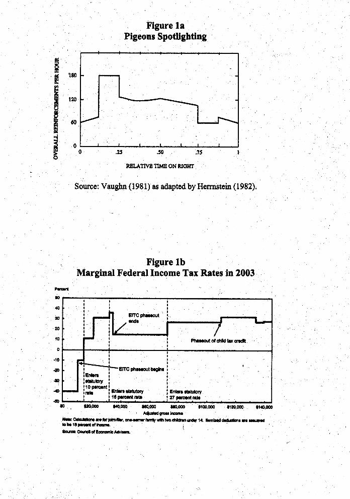
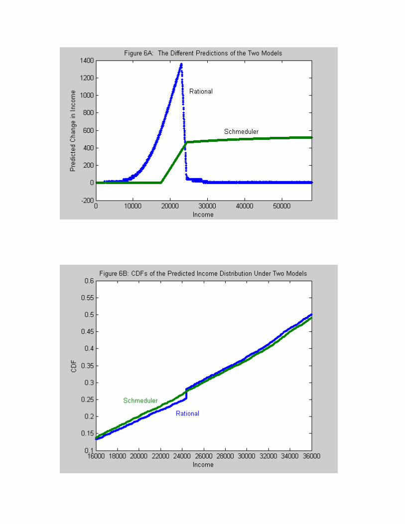
could not take advantage of the full credit.42 Figure 6 illustrates the impact of the introduction of

43 Only children age 17 and under can qualify a taxpayer for the child credit.


the child credit on marginal and average tax rates at different income levels for a taxpayer in

1998. For the purpose of this figure, the taxpayer is assumed to be married with two qualifying

children,43 claim the standard deduction, and have only wage income.

Before 1998, taxpayers with incomes between about $18,000 and $25,000 owed income

tax, and therefore faced a 15 percent marginal tax rate. But beginning in 1998, the child credit

eliminated the entire tax liability for these taxpayers and reduced their marginal tax rate from the

federal personal income tax to zero. Thus, their marginal tax rate fell by 15 percentage points.

All taxpayers with income above $18,000 experienced a reduction in tax liability and therefore a

reduction in average tax rates. The reduction in average tax rates grows with income from

$18,000 until the point at which a taxpayer can use the entire $1000 (2 children X $500) credit.

After that point the reduction in average tax rates falls gradually as the reduction in tax liability

remains $1000, but the denominator in the average tax rate calculation, the person’s income,

rises.

The rational model would predict that the reduction in marginal tax rates would induce

people with income between $18,000 and $25,000 to increase their earnings. We would also

expect to see some bunching at $25,000, the point at which the marginal tax rate jumps from zero

to 15 percent after the reform. Because income effects are generally thought to be close to zero,

we would expect to see little effect on the earnings of people with incomes above $25,000, and

any effect would be a reduction in earnings due to the income effect.

In contrast, the schmeduling model predicts increased work by anyone whose average tax

rate fell – everyone with income above $18,000. In particular, we would expect to see increased


U CL

K

K

= −+

+1

1, (4)

work by people with incomes above $25,000 and no bunching at that point – two predictions that

depart from those of the rational model.

To test these predictions, we use data from the 1997 and 1999 IRS public use Statistics of

Income tax files. These files are based around random samples of individual tax returns, but are

blurred in various ways to protect taxpayer confidentiality. Our basic approach is to examine

whether the change in the distribution of taxpayers by income between 1997 and 1999 looks

more like what would be predicted by the rational model or by the ironing model.

In order to be able to predict how individual behavior will change in response to the

change in budget constraints, we need to model people’s preferences. In particular, given our

interest in the bunching of taxpayers at kink points, we cannot simply predict the change by

multiplying the percentage change in the after-tax share times an elasticity. We follow Diamond

(1998) and Saez (2002) in assuming that preferences take the quasilinear form

where C is consumption and L is labor effort. Under this specification, there is a single

preference parameter, K, which is equal to 1/,, where , is the labor supply elasticity. There is no

income effect in this model. We view this model as the simplest structural analog to elasticity

calculations with a constant elasticity. Although the model is specified in terms of an hours of

work decision, we follow Feldstein (1999) in viewing the behavioral response to taxes more

broadly as any behavior (including compliance, intensity of effort, shifting of compensation into

fringe benefit) that affects taxable income. Thus, , should be interpreted as the elasticity of

taxable income with respect to 1 minus the after tax share.


(L* ) ( ),*K w t= −1 (5)

wwL

t

K K

=−

+( *).

1

11

(6)

The Rational Model

With rational taxpayers, the first order condition from this model is

where t* is the tax rate on the segment of the budget constraint where the taxpayer’s optimum

lies and w is the taxpayer’s wage. By multiplying both sides by wK and rearranging, it is possible

to express w as a function of K and of observable quantities:

Thus given an elasticity, ,, and a distribution of income under a known tax schedule, we can

derive the wage distribution and simulate the distribution of income under any other budget

constraint (We observe pre-tax income, wL*, in our data set; given wL* we know t* since we

know the tax schedule that the taxpayer faces.).

This approach encounters two complications. First, if a taxpayer locates exactly at the

kink point between segments with tax rates of ta and tb, we do not know his exact wage, only that

it lies between the two values that would occur from substituting ta and tb into the equation

above. In practice, only a couple of people in our data set locate exactly at a kink,

and we randomly assign those people to a wage between the two implied by ta and tb, The second

complication is more significant. Because there are almost no people exactly at the kink, the

wage distribution that is implied by taking observed income and plugging it into the equation

44 The complication is not simply that this gap is implausible. Because the gap isdependent on where the kinks are, the implied wage distribution will change when the taxschedule changes, a feature that would be inconsistent with the estimation approach we describebelow.


L wT wL

wLK*

*

*

( )= −

1 (7)

derived above from the first order condition implausibly has a noticeable gap in it – with no one

(except the people exactly at the kink) at wages between the wage implied by ta and the wage

implied by tb..44 Our approach is to assume in our rational model that taxpayers are uncertain

about exactly where the kink is located and so a taxpayer near kink point, k, chooses hours of

work, L, to maximize expected utility where the expectation is over the possible locations of the

kink point. Appendix B derives the perceived marginal tax rate given this assumption. It is

worth emphasizing that by introducing this uncertainty about the location of the kink point into

the rational model we are, in essence, letting the rational taxpayers engage in a bit of

schmeduling. The implication is that if we find evidence of schmeduling behavior when we test

it against this lenient variant of the rational model, it will be even more powerful evidence that

schmeduling is occurring.

The Ironing Model

In the ironing model we assume that taxpayers have the same preferences as they do in

the rational model (equation 4). However, they respond to average tax rates rather than marginal

tax rates. They therefore choose hours, L, to satisfy the following tangency condition

45 In the rational model there is an explicit analytical expression for w. In the ironingmodel, a simple numerical procedure is needed to solve for w.


m S f w S f wm S f w S f w

S R K

S R K

O

O

97 97 97

99 99 99

1

1 1 1

= + − +

= + + − + +

µ ε µ ε σ νµ ε γ µ ε γ σ ν

σ

σ

( , , ) ( ) ( , , , )

( , , ( )) ( ) ( , , ( ), )(8)

instead of the conventional one. In this equation, T(wL*) is total taxes due at income wL*, and

the marginal disutility of effort is equated with the average return to work rather than the

marginal return. Given K and an observed income level, this equation can be used to find w.45

There is no need to introduce uncertainty about the location of the kinks into the ironing model

since the wage distribution implied by ironing does not have a discontinuity at each kink point as

it did in the rational model.

Econometric Model

We now apply the model above to simultaneously estimate the elasticity, ,, and the share

of taxpayers who are schmedulers, s. Let S be a vector in which the ith element equals 1 if the

ith individual is a schmeduler and 0 if the ith individual is rational. The vector of pre-tax

incomes in the two years is given by:

.

Income, m, is determined by the functions :S and :R, which generate an earnings level for a

schmeduler and a rational taxpayer respectively as a function of the tax schedule in each year, f97

and f99, the elasticity, ,, and a vector of taxpayer wages. In the rational case, there is an extra

parameter, Fk, which reflects the amount of uncertainty about where kinks in the schedule are

located. ( is a parameter that describes the amount of nominal wage growth between the two

46 We thank Alberto Abadie for suggesting this formulation of our first identifyingassumption.

47 We currently set FK=$4000, the minimum level that produces a reasonable wagedistribution (i.e. with no sharp reduction in density at the kink points) for all elasticities under 1.We set FO=$2000 based on the evidence in Saez (2002). In principle one could estimate both ofthese parameters as well. Our minimum distance calculation separates the data into 20 bins(defined to each contain 5 percent of the true data) and minimizes the sum of the product of thefractions in each bin in the real data and the fractions in each bin in the simulated data.


years. <F, is a Gaussian random variable representing optimization error; its standard deviation is

FO.

Two key assumptions identify our model. First, the wage distribution in 1999 equals the

wage distribution in 1997 inflated by 1+(. This assumption is similar to the assumption that

underlies most natural experiment studies of tax reforms.46 Second, the probability that a

taxpayer is a schmeduler is the same at all wage levels. While we think this assumption is

unlikely to be strictly true, we think it is a reasonable approximation within the relatively narrow

income range that is our focus with the expansion of the child credit. With sufficient sample

sizes and variation in tax rates, our methodology can be extended to estimate a wage-varying

schmeduling probability.

Our econometric procedure chooses ,, s, and ( along with a mean and variance for the

log wage distribution and then simulates the implied income distribution in each of the two years.

It then searchs over values of the five parameters to find those that minimize the distance

between the simulated income distribution and the observed income distribution.47

Our results are preliminary. Using data generated with known parameter values, our

numerical procedure for finding the parameter values that minimize the distance between the

48 In claiming the child credit, taxpayers could claim only those children age 17 andbelow. We cannot implement this restriction in our data because we do not observe the age ofthe children in the 1997 data. Therefore, we simply assume that all taxpayers with dependentchildren living at home claim the child credit.

49 For these simulations, the standard deviation of the kink error is set at $3000 and theoptimization error is set at $2000.


simulated and actual data frequently selects only a local minimum. We are not yet confident that

we have found the global minimum in the real data.

Data and Results

We limit our sample to married couples with at least two children. For these households,

the introduction of the child tax credit provided a new tax credit of at least $1000.48 Our tax

model consists of the federal income tax (including the EITC) and the OASDI and HI payroll

taxes (modeled as a proportional tax of .0765). We ignore state taxes. To study the full range of

behavioral responses to taxation we define income as adjusted gross income minus itemized

deductions above the standard deduction. In essence, we treat the sum of the standard deduction

and personal and dependent exemptions as a tax bracket with a zero tax rate, rather than

subtracting these amounts from adjusted gross income to define income.

Before turning to results, it is worth asking whether this change in taxes is large enough

to allow us to distinguish between the two models. Figures 6A and 6B demonstrate that the two

models create noticeably different income distributions. Figure 6A takes the 1997 sample and

shows how introducing the child credit in 1997 would have changed the income distribution in

that year under the rational model and under the schmeduling model.49 In particular, it shows

the change in income from introducing the child tax credit plotted against 1997 income with an

50 In percentage terms, the increase in income falls with income above the kink at thestart of the 15 percent bracket. Therefore, if the income growth term, (, is multiplicative, we canseparately identify income growth and schmeduling.


elasticity of 0.40. Under the rational model, taxpayers with incomes between about $10,000 and

$25,000 increase their income. But there is no change for taxpayers who are more than a few

thousand dollars above the new kink at roughly $25,000 (due to uncertainty about the kink point,

a few taxpayers above the kink are affected by the change even in the rational model). Under the

schmeduling model, taxpayers just above the kink have relatively large responses and the dollar

response remains relatively constant for the full range of the income distribution.50 Figure 6B

shows the CDF of income under the two models. There is a noticeable difference in the

schmeduling and rational income distributions between roughly $18,000 and $28,000. In

particular, the rational taxpayers who increase their incomes in response to the reduction in

marginal tax rates produce a deficit of taxpayers between about $18,000 and $25,000 and the

rational CDF is therefore below the ironing CDF over this range. Then the concentration of

taxpayers around the kink point in the rational model causes a sudden jump in the CDF around

$25,000. Just above this income level is where taxpayers experience the largest reductions in

average tax rates. Because of this, the schmeduling CDF falls below the rational CDF as

schmedulers who otherwise would have been in this range increase their incomes in response to

the reduction in their average tax rates.

51 The 1979 increase in the level of earnings subject to the OASDI payroll tax providesanother natural experiment in which the predictions of the ironing model and the rational modeldiffer and in which the methodology presented here could be applied.


Table III shows our results from estimating our model on the actual data. We estimate

that the elasticity of income with respect to the after-tax share is 0.38, that 54 percent of

taxpayers are schmedulers, and that nominal wage growth was 4.7 percent over this period.51

B. The Within-month Pattern of Food Consumption by Food Stamp Recipients

Our second empirical test addresses the spotlighting model, looking at food consumption

by those reeciving food stamps. Our principal hypothesis is that inframarginal food stamp

recipients – those who spend more than the food stamp amount on food during the month –

nonetheless view the cost of spending a dollar of food stamps on food as less than a dollar in

terms of lost consumption of other goods. Before they have exhausted their food stamps, they

respond, in part, to the local price of spending a dollar of food stamps, which they perceive as far

less than one dollar (pure spotlighting would infer a price of zero). That is, during the early

period of the month, they fail to realize that the cost of a marginal dollar of food consumption is

one dollar. Then, after they have exhausted their food stamps and must spend cash for food, they

perceive the true marginal cost of their food. The empirical prediction of the spotlighting model

for food consumption by food stamp recipients is that food consumption should fall through the

month as recipients exhaust their stamps. No such pattern would occur with rational consumers.

A priori, finding evidence of such behavior might seem unlikely, since food stamp recipients get

to play the game many times; every month they get food stamps.

52 We thank Jesse Shapiro for helping us with the data used in this section of the paper. Shapiro (2003) provides evidence suggesting that food consumption by food stamp recipients isconsistent with hyperbolic discounting.

53 Although we describe the cashed out recipients as receiving “cash,” they actuallyreceived their payment in a check.

54 Mathematica evaluated this experiment for the Department of Agriculture and collecteddata on food consumption from about 600 randomly selected food stamp recipients and fromanother 600 who had had their benefits cashed out. Mathematica’s evaluation estimated theimpact of cash out on average food use at home and concluded that it reduced food use at homeby between 5 and 8 percent (Ohls et al 1992) . Whitmore (2002) reevaluated these data, focusingon the difference between marginal and inframarginal consumers as a way to estimate thedeadweight loss from paying in food stamps rather than in cash. She found that inframarginalconsumers do not alter their food consumption when converted to cash, but that “distorted” foodstamp recipients do reduce their consumption, and that they value their stamps at only 80 percentof face value. A similar experiment occurred around the same time in Alabama. However, asWhitmore (2002) discusses, the data from this second experiment are less reliable, both becauseof its limited duration and because caseworkers coached cash recipients not to change their foodconsumption. In addition, we have been unable to learn the institutional details about AFDCpayout dates in Alabama during this period and therefore cannot estimate our model on thesedata. We thank Jesse Shapiro for helping us with these data. Shapiro (2003) provides evidencesuggesting that food consumption by food stamp recipients is consistent with hyperbolic


If we had data only on food consumption by food stamp recipients, however, it would be

hard to distinguish spotlighting from several other hypotheses that could also explain declining

food consumption during the month after benefit payment. For example, myopic consumers

might also have declining consumption throughout the month, as would consumers who consume

a constant minimum level throughout the month but run out of income at the end of the month

(and perhaps consume at a higher level at the beginning of the month because they are hungry

from running out of income at the end of the previous month).52

In order to isolate the pure spotlighting effect, we use data from the 1989-1990 San Diego

food stamp cash out experiment.53 In this experiment, a random sample of the food stamp

caseload had their food stamp checks replaced by an equal amount of cash benefits.54 These data

discounting.

55 Since food data is collected for only one week in this study we scale up the foodconsumption by # days in month/7.


are useful for testing spotlighting because they allow us to distinguish our theory from other

possible explanations for declining food consumption during the month after benefit payment. In

particular, for the myopic, hyperbolic discounting, and food insecurity theories, there is no reason

why the slope of consumption throughout the month should change if stamps were converted to

cash. If spotlighting is occurring, in contrast, we would expect to see a greater decline in

consumption throughout the month for consumers who are paid in food stamps than for

consumers who are paid in cash.

Our base sample consists of all sample members for whom there is complete food

consumption data (a total of 541 receiving food stamps and 537 receiving cash). However, we

want to restrict the sample to inframarginal consumers – those who would consume more than

their food stamps if they received their payment in food stamps.. To identify these consumers we

run a probit regression in the food stamp sample with a dependent variable that is one if the

household consumed more than their food stamps during the survey month.55 The independent

variables are indicators for household size and a fourth degree polynomial in food stamp benefit

level (the food stamp benefit levels in this study are obtained from administrative payment

records). We use this estimated equation to predict a probability of being inframarginal for

households in both the cash and the food stamp group. Then we limit our sample to households

with a predicted probability of 0.95 or above. This results in a sample of 349 in the cash group

and 366 in the food stamp group. In this restricted sample, over 98 percent of households in each

56 The Mathematica data set contains an elaborate set of variables measuring thenutritional value of all of the foods consumed by each household.

57We have explored the sensitivity of our results to including a more elaborate set ofcovariates. As would be expected given the independence between covariates and treatment


group spent more on food than they received in food stamps and the percentages are nearly

identical in the two groups.

We use two dependent variables in our regressions testing our hypothesis: total dollars of

food consumed during the survey week and total calories of food consumed during the survey

week, both measured in natural logarithms.56 Our OLS regression specification is:

(9) ln(food consumption)=$0+$1 (paid in cash)+$2 (days since last AFDC check)+$3(days

since last AFDC check) x (food stamps paid in cash)+$4 (days since last food stamp

check) x (paid in food stamps) +(X +,.

AFDC benefits were paid on the first of the month. Cash recipients received their cashed-out

food stamp payment as part of the same check. In contrast, food stamp recipients received their

food stamp checks at roughly uniform intervals throughout the month. Thus, $2 should capture

the relationship between days since AFDC receipt and food consumption for the entire sample.

$3 should capture any differential relationship between days since AFDC receipt and food

consumption for those in the cashed-out group who also received their food stamp payment with

their AFDC check. $4 is the key parameter for testing our hypothesis. In measures the

relationship between the number of days since food stamp receipt and food consumption for

those receiving food stamps. X is a set of covariates that are assumed not to be affected by the

experiment: dummy variables for calendar month and household size and interactions between

these variables and treatment group.57

assignment (due to the random assignment), the results are quite insensitive to includingadditional covariates.

58 An F-test of the hypothesis that the food stamp coefficients are equal for the cash andstamp samples has a p-value of .17 in the first column and .19 in the second column.


Table 4 shows the results from our regressions. The dependent variable is the log of food

consumption, either measured in dollars (column 1) or in calories (column 2). First, consider

column 1. The point estimates for days since last AFDC check in the first column represents a

0.22 percent per day reduction in consumption or a total decline of about 7 percent over the

month. The coefficients on the interaction between AFDC receipt and payment in cash are

positive. However, neither the coefficient on days since AFDC check receipt or on the

interaction of days since AFDC receipt with cash payment are statistically different from zero

and their coefficients cancel out, suggesting no overall within-month pattern of food

consumption for those receiving all of their benefits in cash.

For those paid in food stamps, the estimates suggests a fairly sharp drop off in

consumption over the food stamp month. The coefficient on the interaction between “days since

food stamp payment” and “payment in stamps rather than checks” is about 0.8 percent per day,

and has a p-value of .051. Thus, individuals receiving payments through food stamps reduce

food consumption by about 24 percent over the month.

This pattern of declining food consumption for those paid in food stamps is not apparent

when food consumption is measured in calories, although the difference between the two food

stamp coefficients (the second and third rows) is similar in the two specifications.58 One possible

explanation for this pattern is that the nutritional content of food purchases changes over the

month as food stamps and money become scarce. This interpretation of the results is consistent


with Whitmore’s (2002) findings for the overall effects of the cash out experiment on food

consumption.

VI. Conclusion

We have argued that schmeduling is likely to be a common form of economic behavior,

that it arises in substantively important areas of economic decision making, and that the welfare

effects of people responding to schmedules rather than to their true schedules are likely to be

large and to have significant policy implications. Moreover, because the conditions that give

rise to schmeduling are found in many economic environments, empirical evidence on how

people respond to schedules in one environment will help us predict how people will react when

faced by schedules in other environments. We have provided two empirical tests of

schmeduling. The tests are not conclusive. However, in both cases the data are consistent with

the presence of a significant amount of schmeduling.

59 By 1976, similar results had been obtained from rats, monkeys, and humans (DeVilliers and Herrnstein, 1976), and the matching law had been shown to apply to variations in thequantity of reinforcement obtained (as opposed to the frequency of reinforcement) and to thedecision of how often to engage in a single activity (as opposed to the choice between twodifferent options). The introductory essays by Rachlin and Laibson (1997) are indispensable inunderstanding this literature.


Appendix A

Herrnstein (1961) demonstrated what he called the matching law: hungry pigeons,

choosing which of two response keys to peck, peck on each lever in proportion to the amount of

reinforcement (food) obtained by pecking on that lever.59 The theory of melioration – that

subjects act to equalize the average return to all choices (keys pecked) – explains matching

behavior (Herrnstein and Vaughn, 1980; Herrnstein, 1982). Such behavior is suboptimal if the

frequency of pecks affects payoffs (such as when there are diminishing returns to pecking on a

given key).

Melioration predicts behavior that incorporates important elements of both ironing and

spotlighting. First, like ironing, melioration predicts that organisms will respond to average

returns. As Herrnstein (1990) explains: “It should soon be evident that the fundamental

difference between matching and utility maximization is that matching is based on average

returns (in utility or reinforcement) over some extended period of activity, while maximization

requires a sensitivity to marginal returns at each moment . . .” Second, like spotlighting,

melioration predicts that organisms will respond to local rather than global payoffs. As

Herrnstein (1982) explains: “[Melioration requires] the organism to respond only to the

difference between local reinforcement rates from individual behaviors. Maximization, in

contrast, requires the selection of the biggest aggregation of reinforcement across behaviors.”

60 Our accounts of these studies are based upon Herrnstein (1982).


Experiments in which melioration and maximization predict different behaviors have almost

always found that behavior follows the predictions of melioration.

Pigeons Ironing. A 1981 pigeon experiment is instructive (Mazur, 1981).60 It involved

periods of darkness possibly yielding food payoffs. The darkness was available at random

intervals, but could be secured only by pecking the then correct key, the two keys being equally

likely. But given darkness, one key paid off with higher frequency than the other. The time to a

new potential darkness interval and the key that would trigger it were then selected at random.

The pigeons pecked far too often on the high payoff frequency key, selecting a ratio close to that

predicted by melioration (in proportion to the frequency of payoff), and far from the more

balanced maximizing ratio. (Half the time, pecking the low-payoff key was the only way to

advance to the next potential darkness period). Pigeons equalized average returns, not marginal

returns.

Humans Spotlighting. Spotlighting arises when current choices affect future payoffs,

hence immediate and marginal payoffs diverge. Psychologists’ experiments have created such

schedules for both humans and pigeons, and shown that both species respond to the immediate

payoffs.

In one such experiment, human subjects were asked to choose between the left and right

arrows on a computer keyboard in exchange for monetary rewards (Herrnstein and Prelec, 1991).

The subjects observed their monetary reward accumulate on a computer screen, which showed

pennies falling. Each time a key was pressed, a penny fell, but a key could not be pressed again

until the penny completed its fall. Pushing the right key caused the penny to fall two seconds


faster than the left key, thus offering a higher instantaneous reward. However, the greater the

fraction of right-key presses in the past 10 choices, the slower the pennies fell, regardless of the

choice. The exact parameters made it optimal to press the left key exclusively. However, almost

all of the subjects exclusively picked the right option after a few trials. Subjects responded to the

immediate reinforcement rate, and did not come close to optimizing against the true schedule.

Pigeons Spotlighting. When subjects – be they pigeons or humans – are presented with

complex schedules, it can be almost impossible to discern marginal payoffs. Figures 1a and 1b

show the schedules respectively of a pigeon reward experiment (Vaughn, 1981) and of a married

U.S. taxpayer with two children (Council of Economic Advisors, 2003); they look like Rorshach

Test equivalents. In the pigeon experiment payoffs depended on pecks in the previous four

minutes. The highest payoffs came if the right key was pecked between 12.5 percent and 25

percent of the time, the lowest if it was pecked between 75 percent and 87.5 percent of the time.

However, actual delivery of the rewards occurred mostly after a peck on the right key. The three

pigeons in this experiment all ended up spending between 75 and 80 percent of their time on the

right key, spotlighting as they responded to instantaneous payoffs – and found, alas, the global

minimum.

Our empirical section analyzes human response to complex schedules, though none as

complex as the one in Figure 1b. Interestingly, even the Council of Economic Advisors – which

did not have to peck or earn in real time to discover it – could not present this schedule correctly.

The income level at which the phase-out of the EITC begins is mislabeled.


Appendix B. Spotlighting Losses With Continuous Consumption

We compute spotlighting’s deadweight losses when consumption is continuous, as it is

say for water. Let x[p(t)] be the consumer’s instantaneous demand at time t, and T be the length

of the accounting period. Define the cumulative demand through time t as F(t) = . x p s dst

[ ( )]0∫

The price at time t, p(t), equals p1 if F(t)<k and equals p2 if F(t)>= k (where k is the kink point –

the level of cumulative demand at which the price switches from p1 to p2).

Total consumption under spotlighting is , where is theF T x p dt x p dtt

t

T

( ) ( ) ( )>

>

= +∫ ∫10

2 >t

amount of time it takes to exhaust the first price-segment and therefore solves . x p dt kt

( )>

10

=∫

This relationship implies that , or . Therefore, x p t k( ) >1 = >

( )t

kx p

=1

, which implies that total consumption under spotlighting is:F T x p dt x p dt

kx p

kx p

T

( ) ( ) ( )( )

( )

= +∫ ∫10

2

1

1

.F T x pk

x px p T x p

kx p

( ) ( )( )

( ) ( )( )

= + −11

2 21

Total consumption for a rational consumer is simply F T x p dt x p TT

( ) ( ) ( ) .= =∫ 20

2

Subtracting total rational consumption from total spotlighting consumption yields the excess

consumption under spotlighting: . Intuitively, excessive consumption rises with k,kx px p

1 2

1−

( )( )

because a larger k implies that the consumer is responding to the wrong price a greater fraction of

the time. In addition, excess consumption is larger the bigger the gap between demand at p2 to

61Moving the initial x(p1) to the inside of the integral yields an expression that is quitesimilar to the expression for the amount of over-consumption, and, not surprisingly,demonstrates that the same conditions for when over-consumption will be high apply todeadweight loss as well – deadweight loss rises with k and with the elasticity of demand.


demand at p1. In contrast if consumption is completely inelastic and x(p2) equals x(p1) there is no

excess consumption.

Integrating excess consumption between the two prices yields the deadweight loss:

, where represents the amount of time that the[ ]DWLk

x px p x z dz

p

p

= −∫( )( ) ( )

11

1

2 kx p( )1

individual is overconsuming, and the integral gives the instantaneous DWL during these periods

of overconsumption.61

C The Mirrlees Problem when Taxpayers Re-spond to Average Tax Rates

We follow the notation and approach of Diamond (1998). n is the worker�sskill level. x(n) represents consumption by a person with skill level n. y(n) is

labor supply in percentage terms of a person with skill level n. Utility takesthe quasilinear form

u(x; y) = x(n) + v(1� y); (C-1)

where v(1 � y) is the disutility of e¤ort. The social planner�s objective is tomaximize social welfare,

max

n1Zn0

G fU [x (n) ; y (n)]g f (n) dn; (C-2)

subject to the budget constraint,

n1Zn0

T [ny (n)] f (n) dn � E; (C-3)

and to an incentive-compatability constraint for each individual. In these lasttwo equations, G fUg is the social welfare function, f(n) is the skill distribu-tion, E is government spending, and T [ny (n)] represents taxes as a function of

earnings.

With these de�nitions, the expression for utility can be rewritten as:

u(x; y) = x+ v (1� y) (C-4)

= ny � T [ny(n)] + v(1� y): (C-5)

The �rst order condition for individual optimization under the standardmodel is

v0 [1� y(n)] = n f1� T 0 [ny(n)]g : (C-6)

However when the taxpayer is an ironer and instead responds to average taxrates, the FOC becomes

v0 [1� y(n)] = n�1� T [ny(n)]

ny(n)

�: (C-7)

53

C.1 The Mirrlees First Order Condition

To solve this problem, note that equation C-7 can be rewritten as

T [ny(n)] = y(n) [n� v0[1� y(n)]] (C-8)

and substituted for T [ny(n)] in the social welfare objective. This substitutionallows us to solve the Mirrlees problem by forming a simple Lagrangian ratherthan the Hamiltonian that is necessary in the standard version of the problem:

L = G [v + yv0]� p [y(n)v0[1� y(n)]� ny(n)] f(n)dn: (C-9)

Di¤erentiate with respect to y(n) to get

G0(u) (�yv00)� p [v0 � yv00 � n] = 0: (C-10)

To interpret this expression, it is useful to substitute for v0 and v00. We

can eliminate v0 using v0 = nh1� T (ny)

ny

ifrom equation C-7. To eliminate v00,

we �rst derive an expression for the elasticity of labor supply with respect to1 minus the perceived after tax wage. Note that from taking the derivative of

the schmeduling FOC (equation C-7) with respect to nh1� T (ny)

ny

iwe get

dy

dn(1� T (ny)ny )

=�1v00: (C-11)

The elasticity therefore equals

e(n) =dy

dn(1� T (ny)ny )

n(1� T (ny)ny )

y=�v0yv00

; (C-12)

which is the same as in the standard case. Rearranging equation C-10 andsubstituting we get

54

G0(u) =p [v0 � yv00 � n]

(�yv00) (C-13)

= p

�e+ 1 +

n

yv00

�= p

�e+ 1 + n

v0

yv001

v0

�

= p

24e+ 1� ne 1

nn1� T [ny]

ny

o35

= p

�e+ 1� e 1

1�ATR

�1� G

0(u)

p= �e+ e 1

1�ATR�1� G

0(u)

p

�1

e=

1

1�ATR � 1

ATR

1�ATR =

�1� G

0(u)

p

�1

e(C-14)

C.2 Perturbation Approach

The same result can be obtained using the perturbation approach of Saez(2001).At the optimum, the revenue gain from a small increase in taxes, weighted bythe average social welfare weight, must equal the welfare loss for the people onwhom the taxes were increased. Let M be the mechanical revenue e¤ect, B bethe behavioral revenue e¤ect, p be the average welfare weight, and G0(u) be thewelfare weight on the people whose taxes are being increased:

p(M +B) = G0(u)M: (C-15)

Given ironing, if we raise a person�s average tax rate by dt, we have thefollowing:

Direct revenue e¤ect: M = nydt:

Behavioral revenue e¤ect: e = dRd(1�ATR)

(1�ATR)R , soB = dR = eR d(1�ATR)

1�atr =

e(ATR)(ny) �dt1�atr = �

ATR1�ATR (ny)edt:

55

Welfare e¤ect: �G0(u)nydt:

Plugging these components into equation C-14, we get:

p

�nydt� ATR

1�ATR (ny)edt�

= �G0(u)nydt (C-16)

1� e ATR

1�ATR = �G0(u)

p

ATR

1�ATR =1

e

�1� G

0(u)

p

�:

C.3 Asymptotic tax rate

The asymptotic tax rate can be derived directly from the FOC under the as-

sumption that G0(u)p ! 0 asymptotically. This yields:

ATR =MTR =1

e+ 1(C-17)

More generally, the optimal rate above a given income level can be deter-mined as in Saez (2001) by de�ning �g as the ratio of the average social welfareweight on those above the given income level to the overall average. Then theoptimal rate on high-income taxpayers becomes

ATR =MTR =1� �g

e+ 1� �g (C-18)

C.4 Numerical Simulations

Traditionally, empirical simulations of the optimal tax schedule have relied onnumerical solution of the Mirrlees di¤erential equations. However, Saez hasproposed an alternate numerical approach based directly on the �rst order con-dition that is much easier (and appears to be more reliable) than solving thedi¤erential equations. Under the Saez method, one guesses an initial tax sched-ule (say a 25 percent marginal rate at all income levels), �nds the optimum foreach skill level under that tax schedule, and then generates a new tax scheduleby calculating the value of the right hand side of the FOC at this new set ofoptima. One then solves for either the marginal tax rate (in the traditionalMirrlees problem) or the average tax rate (when taxpayers are responding toaverage tax rates). One repeats this process by using the new tax schedule inplace of the initial tax schedule until the process converges.

56

For comparability, we follow Saez (2001) in our data construction and as-sumptions. We assume that utility takes the quasilinear form, U = C + L1+K

1+K ;and that social welfare is ln(u): We take the earnings of married couples fromthe 1992 Statistics of Income public use tax �le and invert the �rst order con-dition to obtain the skill distribution, given the assumption that people faced a�at 25 percent tax schedule. We also impose a lower-bound on the skill level atthe skill level implied by a 1992 earnings level of $5000. We assume that gov-ernment (non-transfer) spending is 20 percent of actual 1992 pre-tax earningsfor our sample of married taxpayers.One subtlety in the simulations for the ironing model is the treatment of

lump-sum transfers. Would providing a lump-sum transfer to all workers re-duce average tax rates and increase work? Our assumption is that lump-sumtransfers do not a¤ect people�s perceptions of their return to work. However,without imposing further constraints, this assumption about lump-sum transfers(along with our chosen utility function) would produce an optimum with a largelump sum tax and a hugely negative tax rate at the lowest income level corre-sponding to positive earnings. We avoid this unreasonable result by assumingthat ten percent of the population is made up of non-workers. This produces anendogenously chosen positive level of lump-sum transfers at zero income. Moregenerally, the simple Mirrlees model with quasi-linear preferences is not a verygood model for thinking about the labor force participation decision of peopleat very low skill levels. Models such as Saez (2002b) and Liebman (2002) thatexplicitly consider the extensive margin are more appropriate.

57


[ ]E U L wl wL t p k k t t dk wl wL tL

KH H L

wL

L

K

( ) ( ) ( ) ( ) ( ) ( ( )) ( )= − + − + − − −+−∞

+

∫Φ Φ1 1 11

1

[ ]L Y t Y t Y t Y tH L H LK= − + − − + ′ − − ′ − +( ) ( )( ) ( ) ( ) .1 1 1 1 12 2

11Φ Φ Φ Φ

Appendix D: The Rational Model with Uncertainty about the Location of the Kink

We assume that a taxpayer near kink point, k, chooses hours of work, L, to maximize

expected utility where the expectation is over the possible locations of the kink point.

(D1) [ ] [ ]E U L p k wL kt t wL k dk p k wL t wL dkL

KL H

wL

LwL

K

[ ( )] ( ) ( ) ( ) .= − − − + − −+−∞

∞ +

∫ ∫1

1In this equation, tL is the tax rate on the segment of the tax schedule just below the kink point at

k, tH is the tax rate on the segment of the tax schedule that starts at k, and p(k) is the probability

distribution function of k. The first term in the equation is after-tax income (consumption) when

the kink point is below wL and the second term is after-tax income when the kink point is above

wL . If we further assume that the uncertainty is distributed normally with mean at the true kink

point and standard deviation Fk, the expression can be rewritten as:

(D2)

where M is the normal CDF. The first order condition is (surpressing the argument of M):

(D3) 0 1 1 1 1 12 2= ′ − + − + − − ′ − − − −Φ Φ Φ Φ Φw L t w t w t w L t w t LH H L L LK( ) ( ) ( ) ( ) ( )

Multiplying through by L and replacing wL with Y (the income observed in the data), we can

express L as a function of observed quantities:

(D4)

We can then determine w as Y/L. Thus, in our rational model, we have two preference

parameters K (the inverse of the labor supply elasticity) and Fk, (the amount of uncertainty


around the location of kink points). It can be shown that the marginal tax rate perceived by the

taxpayer near the kink point between ta and tb in this model is a weighted average of ta and tb:

(D5) mtr Y t Y t Ya b( ) ( ( )) ( ).= − +1 Φ Φ


References

Auerbach, Alan J. and Laurence J. Kotlikoff (1985). The Efficiency Gains from Social SecurityBenefit-Tax Linkage. NBER Working Paper 1645.

Auten, Gerald, and Robert Carroll (1997). The Effects of Income Taxes on Household Behavior. Office of Tax Analysis, U.S. Department of the Treasury.

Bernheim, B. Douglas and Antonio Rangel (2002). Addiction and Cue-conditioned CognitiveProcesses. NBER Working Paper 9329.

Bises, Bruno (1990). Income Tax Perception and Labour Supply in a Sample of IndustryWorkers, Public Finance, 1:3-17.

Brannas, Kurt and Niklas Karlsson (1996). Estimating the Perceived Tax Scale within a LaborSupply Model. Economic Letters, 52:75-79.

Break, George (1957). “Income Taxes and Incentives to Work: An Empirical Study,” American

Economic Review, 47:529-549.

Brown, C.V. (1968). Misconceptions About Income Tax and Incentives. Scottish Journal ofPolitical Economy, February: pp1-12.

Burtless, Gary and Robert Moffitt (1984). The Effect of Social Security Benefits on the LaborSupply of the Aged. In Henry Aaron and Gary Burtless, editors. Retirement andEconomic Behavior. Brookings Institution: Washington, 135-174.

Courant, Paul N., Edward M. Gramlich, and Daniel L. Rubinfeld (1979). The StimulativeEffects of Intergovernmental Grants: Or Why Money Sticks Where It Hits. InMieszkowski, Peter, and William H. Oakland, editors, Fiscal Federalism and Grants-in-Aid. Washington, D.C.: Urban Institute. Pp. 5-21.

de Bartolome, Charles A.M. (1995). “Which Tax Rate Do People Use: Average or Marginal?” Journal of Public Economics, 56:79-96.

de Villiers, Peter A. and Richard J. Herrnstein. (1976). “Toward a Law of Response Strength,” Psychological Bulletin, 83:1131-1153. Reprinted in Richard J. Herrnstein, The MatchingLaw: Papers in Psychology and Economics , edited by Howard Rachlin and David I.Laibson, (Cambridge, Harvard University Press), 1997.

Diamond, Peter (1998). “Optimal Income Taxation: An Example with a U-Shaped Pattern ofOptimal Marginal Tax Rates,” American Economic Review, 88, 83-95.


Dickert, S., S. Hauser, and J.K. Scholz (1994). Taxes and the Poor: A Microsimulation Study ofImplict and Explicit Taxes. National Tax Journal 47: 76-97.

Eissa, Nada (1995). Taxation and Labor Supply of Married Women: the Tax Reform Act of1986 as a Natural Experiment. NBER Working Paper No. 5023.

Eissa, Nada and Jeffrey Liebman (1996). The Labor Supply Impact of the Earned Income TaxCredit. Quarterly Journal of Economics, 111, 605-637,

Feldstein, Martin (1995). The Effect of Marginal Tax Rates on Taxable Income: A Panel Studyof the 1986 Tax Reform Act. Journal of Political Economy, 103:551-572.

Feldstein, Martin (1999). Tax Avoidance and the Deadweight Loss of the Income Tax, Review ofEconomics and Statistics, 81: 674-680.

Friedberg, Leora (2000). The Labor Supply Effects of the Social Security Earnings Test. Reviewof Economics and Statistics, 82: 48-63.

Friedman, Lee S. (2002). Bounded Rationality versus Standard Utility-Maximization: A test ofEnergy Price Responsiveness. In Rajeev Gowda and Jeffrey C. Fox, editors, Judgments,Decisions, and Public Policy. Cambridge: Cambridge University Press.

Fujii, Edwin T. and Clifford B. Hawley (1988). On the Accuracy of Tax Perceptions, Review ofEconomics and Statistics, 344-347.

Giannarelli, L. and E. Steuerle (1995). It’s Not What You Make, It’s What You Keep: Tax RatesFaced by AFDC Recipients. Paper presented at the APPAM Annual ResearchConference.

Goolsbee, Austin (2000). It’s Not About the Money: Why Natural Experiments Don’t Work Onthe Rich. In Slemrod, Joel (editor), Does Atlas Shrug? The Economic Consequences ofTaxing the Rich. Cambridge University Press, Cambridge.

Grogger, Jeff and Charles Michalopoulous (1999). Welfare Dynamics Under Time Limits. NBER Working Paper 7353.

Gruber, Jonathan and Peter Orszag (1999). What to Do About the Social Security EarningsTest? Center for Retirement Research Issue Brief 1999:1.

Gruber, Jonathan and Emmanuel Saez (2002). “The Elasticity of Taxable Income: Evidence andImplications,” Journal of Public Economics, 84:1-32.

Hausman, Jerry (1981). “Labor Supply” in Henry Aaron and Joseph Pechman (editors) HowTaxes Affect Economic Activity (Brookings, Washington, DC).


Heckman, James (1983). “Comment on Stochastic Problems in the Simulation of Labor Supply”in Martin Feldstein (editor) Behavioral Simulation Methods in Tax Policy Analysis.

Heim, Bradley T. and Bruce D. Meyer (2003). Work Costs and Nonconvex Preferences in theEstimation of Labor Supply Models. NBER Working Paper 9429.

Barthold, Thomas A., Thomas Koerner, and John F. Navratil (1998). Effective Marginal Tax Rates Under the Federal Individual Income Tax: Death by One Thousand Pin Pricks?National Tax Journal, 51: 553-564.

Herrnstein, Richard J. (1961). “Relative and Absolute Strength of Response as a Function ofFrequency of Reinforcement.” Journal of the Experimental Analysis of Behavior, 4: 267-272. Reprinted in Richard J. Herrnstein, The Matching Law: Papers in Psychology andEconomics , edited by Howard Rachlin and David I. Laibson, (Cambridge, HarvardUniversity Press), 1997.

Herrnstein, Richard J. and Heyman, G. M.(1979). “Is Matching Compatible with Reinforcement Maximization on Concurrent Variable Interval, Variable Ratio?” Journal of theExperimental Analysis of Behavior, 31, 209-223.

Herrnstein, Richard J. (1982). “Melioration as Behavioral Dynamism.” Reprinted in Richard J.Herrnstein, The Matching Law: Papers in Psychology and Economics , edited by HowardRachlin and David I. Laibson, (Cambridge, Harvard University Press), 1997.

Herrnstein, Richard J. (1990). “Rational Choice Theory: Necessary but Not Sufficient.” American Psychologist, 45: 356-367. Reprinted in Richard J. Herrnstein, The MatchingLaw: Papers in Psychology and Economics , edited by Howard Rachlin and David I.Laibson, (Cambridge, Harvard University Press), 1997.

Herrnstein, Richard J. (1991). “Experiments on Stable Suboptimality in Individual Behavor.”American Economic Review (May), 81: 360-364.

Herrnstein, Richard J. and Drazen Prelec (1991). “Melioration: A Theory of Distributed Choice,”Journal of Economic Perspectives, 5:137-156.

Herrnstein, Richard J. and Vaughan, w., Jr. (1980). “Melioration and Behavioral Allocation.” InJ.E.R. Staddon (ed.), Limits to Action: The Allocation of Individual Behavior (New York:Academic Press).

Hines, James R. and Richard H. Thaler (1995). The Flypaper Effect. Journal of EconomicPerspectives, 9: 217-226.

Keeler, Emmet and J.E. Rolph (1988). The Demand for Episodes of Treatment in the HealthInsurance Experiment. Journal of Health Economics, 7: 337-367.


Kling, Jeffrey, Jeffrey Liebman, and Larry Katz (2003). Bullets Don’t Got No Name: Consequences of Fear in the Ghetto. Forthcoming in Thomas Weisner (editor), Discovering Successful Pathways, University of Chicago Press

Kotlikoff, Laurence J. (1995). Privatization of Social Security: How It Works and Why It Matters, Tax Policy and the Economy, 10: 1-32.

Laibson, David (1997). Golden Eggs and Hyperbolic Discounting. Quarterly Journal ofEconomics, 62: 443-477.

Liebman, Jeffrey (1996). The Impact of the Earned Income Tax Credit on Labor Supply andTaxpayer Compliance. Harvard University Phd Thesis.

Liebman, Jeffrey (1998). The Impact of the Earned Income Tax Credit on Incentives and theIncome Distribution, Tax Policy and the Economy, volume 12.

Liebman, Jeffrey (2002). The Optimal Design of the Earned Income Tax Credit in Bruce D. Meyer and Douglas Holtz-Eakin, editors, Making Work Pay: The Earned Income Tax Credit and Its Impacton American Families (New York: Russell Sage Foundation Press).

MaCurdy, Thomas, David Green, and Harry Paarsh (1990). “Assessing Empirical Approachesfor Analyzing Taxes and Labor Supply,” Journal of Human Resources, 25: 415-490.

Mazur, J.E. (1981). “Optimization Theory Fails to Predict Performance of Pigeons in a Two-Response Situation.” Science, 214: 823-825.

Meyer, Bruce D. and Rosenbaum, Dan T. (2001). Welfare, the Earned Income Tax Credit, andthe Labor Supply of Single Mothers. Quarterly Journal of Economics. 116: 1063-1114.

Meyer, Bruce D. (2002). Labor Supply at the Extensive and Intensive Margins: The EITC,Welfare, and Hours Worked. American Economic Review, May.

Meyers, Marcia K, Bonnie Glaser, and Karin MacDonald (1998). On the Front Lines of WelfareDelivery: Are Workers Implementing Policy Reforms? Journal of Policy Analysis andManagement, 17:1-22.

Oates, Wallace (1979). Lump-sum Intergovernmental Grants Have Price Effects. InMieszkowski, Peter, and William H. Oakland, editors, Fiscal Federalism and Grants-in-Aid. Washington, D.C.: Urban Institute. Pp. 23-30.

Pollack, Harold and Richard Zeckhauser (1996). Budgets as Dynamic Gatekeepers, ManagementScience, 42: 642-658.


Rachlin, Howard and David I. Laibson (1997). “Introduction,” in Richard J. Herrnstein, The Matching Law: Papers in Psychology and Economics , edited by Howard Rachlin andDavid I. Laibson, (Cambridge, Harvard University Press).

Romich, Jennifer and Thomas Weisner (2002). How Families View and Use the Earned Income Tax Credit, in Bruce Meyer and Douglas Holtz-Eakin editors, Making Work Pay. RussellSage Foundation, New York.

Rosen, Harvey S. (1976). Taxes in a Labor Supply Model with Joint Wage-Hours Determination, Econometrica, 44:485-507.

Saez, Emmanuel (1999). The Effect of Marginal Tax Rates on Income: A Panel Study ofBracket Creep, Journal of Public Economics.

Saez, Emmanuel (2001). Using Elasticities to Derive Optimal Income Tax Rates. Review ofEconomic Studies, 68: 205-229.

Saez, Emmanuel (2002a). Do Taxpayers Bunch at Kink Points? Mimeo UC Berkeley.

Saez, Emmanuel (2002b). Optimal Income Transfer Programs: Intensive Versus ExtensiveLabor Supply Responses. Quarterly Journal of Economics, 117: 1039-1073.

Simon, Herbert A. (1978). Rationality as Process and as Product of Thought. AmericanEconomic Review Papers and Proceedings, 68:1-16.

Slemrod, Joel (1990). Do Taxes Matter?. MIT Press, Cambridge, MA.

Thaler, Richard H. (1985). Mental Accounting and Consumer Choice. Marketing Science 4:199-214.

Thaler, Richard H. and H.M. Shefrin (1981). An Economic Theory of Self-control. Journal ofPolitical Economy 89: 392-406.

Tversky, Amos and Daniel Kahneman (1974). Judgment Under Uncertainty: Heuristics andBiases. Science. 185: 1124-1131.

Vaughn, W., Jr. (1981). “Melioration, matching, and maximization.” Journal of theExperimental Analysis of Behavior, 36: 141-149.

Table IFive Examples of Conditions that Give Rise to Schmeduling

Non-linear pricing

Com

plexity

Frequent revisions

Delayed Payoffs

Bundled C

onsumption

Nonstationary environm

ent

Schedule heterogeneity

Obscure units

False signals

Tax schedules X X X X ? X X X

Public assistance benefit formulas X X X ? ? X ?

Utility pricing X X X X X X X X ?

Richard’s parking tickets X X X X

Non-linear pricing of consumer goods X X X ? ? X

Note: X means that the condition is usually present for that example. ? means that thiscondition is sometimes present and sometimes not in that example.

Table IIDeadweight Loss in the Two Models with Elasticity of 0.4

(billions of dollars)

Taxable Income Revenue Deadweight Loss

Schmeduling 4233.3 974.7 56.7

Rational 4019.9 913.4 109.0

Table IIIParameter Estimates from the Econometric Model of the Introduction of the Child Credit

Elasticity 0.38

Share of sample that are schmedulers 0.54

Nominal wage growth 0.047

Notes. Standard deviation of optimization error is set to $2000. Standard deviation ofuncertainty around the kink is set at $4000.

Table IV: Regression Results for the Within-Month Pattern of Food Consumption by Food Stamp Recipients

Dependent Variable

Log of food consumption in dollars

(1)

Log of food consumption in calories

(2)

Days since lastAFDC check

-.00216(.00417)

-.00384(.00424)

Days since lastAFDC check interacted withFood Stamps paid in cash

.00192(.00566)

.00733(.00575)

Days since last Food Stampcheck (for those paid instamps)

-.00761(.00390)

-.00205(.00397)

R2 0.27 0.30

Sample size 715 715

Notes: Regressions also include indicator variables for calendar month, household size, andexperimental group. Robust standard errors in parentheses.

Monopolist Good

AllOther

Goods$

Consumers' Budget Constraint in Monopolist CaseFigure 2a

A

K

B

Slope p2*

Quantity

Net Revenue

Feasibility

Rational

LO

Feasibility

Rational

HI

Feasibility

Ironing

HI

Monopolist CaseFigure 2b

F

E

R

D

S

G

T

Se

V

Quantity

Net Revenue

Feasibility

Rational

LO

Feasibility

Rational

HI

Feasibility

Ironing

HI

Ramsey PricingFigure 3

B

D

A

C

Pre-Tax Income

Post-TaxIncome

Schmeduling in the Optimal Income TaxFigure 4

C

BA

F

Quantity

Price

Deadweight Loss from Spotlighting

Figure 5

BA

D

E

F

G

H

I J

Kp1

p2

Z

C

QspotQrat Qtot

Figure 6Change in Average and Marginal Tax Rates from Introduction of Child Credit

-16

-14

-12

-10

-8

-6

-4

-2

0

025

0050

0075

0010

000

1250

015

000

1750

020

000

2250

025

000

2750

030

000

3250

035

000

3750

040

000

4250

045

000

4750

050

000

5250

055

000

5750

060

000

6250

065

000

6750

070

000

Adjusted Gross Income

Perc

enta

ge P

oint

s

MTRATR

0 50,000 100,000 150,000 200,000 250,000 300,000-1

-0.8

-0.6

-0.4

-0.2

0

0.2

0.4

0.6

0.8

1

earnings

aver

age

tax

rate

Figure 7A: Optimal Average Tax Rates Given Ironing

elas=0.8

elas=0.5

elas=0.2

0 50,000 100,000 150,000 200,000 250,000 300,0000

0.1

0.2

0.3

0.4

0.5

0.6

0.7

0.8

earnings

mar

gina

l tax

rate

Figure 7B: Optimal Marginal Tax Rates

ironing: elas=0.8

ironing: elas=0.5

rational: elas=0.5

Date post:	18-Jan-2019
Category:	Documents
Upload:	halien
View:	222 times
Download:	0 times

Schmeduling Jeffrey B. Liebman and Richard J. Zeckhauser … · Schmeduling Jeffrey B. Liebman and...

Documents