SCHOOL ACCOUNTABILITY AND TEACHER Mtsass/pdfs/feng figlio sass revised 20160624 jue... · 1 SCHOOL...

1

SCHOOL ACCOUNTABILITY AND TEACHER MOBILITY

Li Feng Texas State University

David Figlio

Northwestern University and NBER

Tim Sass Georgia State University

Current version: June 24, 2016

This is a considerably updated version of a paper with the same name that first appeared as NBER working paper 16070 (June 2010). We are grateful to the U.S. Department of Education (via the National Center for the Analysis of Longitudinal Data in Education Research), National Science Foundation and National Institutes of Child Health and Human Development for research support and to the Florida Department of Education for providing the data for this analysis. We also wish to thank seminar participants at Indiana, Northwestern, Oregon, Wisconsin, and the Swedish Research Institute for Industrial Economics, as well as conference participants at the American Education Finance Association, Association for Public Policy Analysis and Management, Society for Research on Educational Effectiveness, and Southern Economic Association meetings, for helpful comments. We alone are responsible for any errors in analysis or interpretation. The results reported herein do not necessarily reflect the views of the Florida Department of Education or of our funders.

2

I. Introduction

School accountability -- the process of evaluating schools based on performance of their

students and holding the schools responsible for student outcomes -- is becoming increasingly

prevalent around the world. Accountability systems typically provide direct incentives in the

form of explicit rewards or sanctions associated with student performance. In addition,

accountability systems may engender social pressure, since a school’s constituents have both

educational and financial1 reasons to influence low-performing schools to improve. There exists

considerable evidence that schools are changing as a result of accountability, but the evidence

regarding the effects on teachers – the people charged with carrying out school policies and

practices -- is extremely limited. This paper makes use of detailed individual teacher-level data

from Florida to gauge the degree to which these direct and indirect forms of accountability

pressure affect the occupational choices of teachers.

There is strong reason to believe that accountability pressure influences the ways in

which educators carry out their jobs. The weight of the evidence suggests that accountability

systems tend to improve the outcomes of low-performing students (see, e.g., Ballou and

Springer, 2008; Carnoy and Loeb, 2002; Chakrabarti, 2007; Chiang, 2009; Dee and Jacob, 2011;

Figlio and Rouse, 2006; Hanushek and Raymond, 2004; Ladd and Lauen, 2009; Reback,

Rockoff and Schwartz, 2011; Rockoff and Turner, 2010; Rouse et al., 2013; West and Peterson,

2006; Wong, Cook and Steiner, 2010), implying that these systems are changing the ways in

which schools do business.2 Rouse et al. (2013) document a number of the ways in which

accountability pressure has changed school instructional policies and practices in Florida’s low-

1 School accountability ratings are capitalized into housing prices (Figlio and Lucas, 2004), which in turn affect the property tax base for schools, and they affect a school’s ability to raise voluntary contributions (Figlio and Kenny, 2009). 2 Craig, Imberman, and Perdue (2013) identify some ways in which school accountability systems influence school resource allocations.

3

performing schools, and relate these instructional policy and practice changes to increased

student performance. The same pressures to improve efficiency also may lead to other changes

in the school environment; Booher-Jennings (2005), Krieg (2008), Neal and Schanzenbach

(2010), Ozek (2010) and Reback (2008) show that schools subject to accountability pressure tend

to concentrate attention on some students at the apparent expense of others. Some schools have

responded by differentially reclassifying low-achieving students as learning disabled so that their

scores will not count against the school in accountability systems (see, e.g., Cullen and Reback,

2007; Figlio and Getzler, 2007; Jacob, 2005).3 Figlio and Winicki (2005) suggest that Virginia

schools facing accountability pressures altered their school nutrition programs on testing days to

increase the likelihood that students will do well on the exams, and Figlio (2006) indicates that

schools differentially suspend students at different points in the testing cycle in an apparent

attempt to alter the composition of the testing pool. Jacob and Levitt (2003) find that teachers

are more likely to cheat when faced with increased accountability pressure.

With school accountability changing the ways in which schools are operating, it seems

natural to believe that these systems would influence the teacher labor market. School

accountability systems may influence the desirability of certain teaching jobs, and may also

affect the willingness of schools to retain certain teachers. From a theoretical perspective, the

effects of accountability pressures on the teacher labor market are ambiguous. On the demand

side, in order to avoid sanctions and/or the stigma associated with being designated as a “failing”

school, schools could increase their efforts to identify low performing teachers and remove them

from their classrooms. On the supply side, accountability pressure and associated changes in

school policies could lower the net benefit of teaching in a school by reducing teacher discretion

3 Chakrabarti (2007), however, does not find that schools respond in this way.

4

over curriculum or teaching methods. Likewise, the potential stigma from teaching in a “failing”

school could lead some teachers to seek employment at other schools. On the other hand, the

resources that often accompany sanctions (e.g. reading coaches, enhanced training for teachers,

etc.) could reduce the non-monetary costs associated with working in low-performing schools

and actually increase teacher retention.

A number of recent papers have analyzed the determinants of teacher mobility and

attrition (Boyd et al., 2005, 2006; Feng, 2009; Hanushek et al., 2004; Imazeki, 2005; Jackson,

2012, 2013; Krieg, 2006; Podgursky et al., 2004; Scafidi et al. 2007). However, the literature

relating recent public policy changes regarding teachers, such as accountability pressures, to

teachers’ labor market decisions has been much spottier. Boyd et al. (2008) explore the

responses of teachers to the introduction of mandated state testing in New York State. They find

that teacher turnover in fourth grade, the critical accountability year in New York, decreased

following the introduction of testing, and that entrants into fourth grade were more likely to be

experienced teachers than had previously been the case. Clotfelter et al. (2004) evaluate how

North Carolina’s accountability system influenced the ability of schools serving low-performing

students to attract and retain high-quality teachers. They find that the introduction of the

accountability system exacerbated teacher turnover in these schools, though it is less evident that

accountability led to lower qualifications of the teachers serving low-performing students. Both

of these papers carefully describe the accountability systems in their states, but because they

evaluate accountability systems that affected all schools within a state, it is difficult to derive

causal inference from their analyses.

In this paper, we exploit a major rule change in Florida’s school accountability system

that took place in the summer of 2002 to identify the effects of changing school accountability

5

pressures on teacher mobility between schools and occupations. Florida had graded every school

in the state on a scale from “A” to “F” since the summer of 1999, based on proficiency rates in

reading, writing and mathematics. Florida’s system of school accountability, called the A+ Plan

for Education, included a series of rewards and sanctions for high-performing and low-

performing schools. Florida’s system has become a model for the rest of the United States, with

a number of states and localities, ranging from Arizona to Indiana to North Carolina to New

York City4, adopting accountability systems that mirror many key features of the policy. In

2002, the state dramatically changed its grading system to both recalibrate the acceptable student

proficiency levels for the purposes of school accountability and to introduce student-level

changes in test scores as an important determinant of school grades. Using student-level micro-

data to calculate the school grades that would have occurred absent this change, we demonstrate

that half of all schools in the state experienced an accountability “shock” due to this grading

change, with some schools receiving a higher grade than they would have otherwise received and

other schools receiving a lower grade than would have otherwise occurred. Furthermore, some

schools were shocked downward to receive a grade of “F”, which no school in the state had

received in the prior year of grading. These grading shocks provide the vehicle for identification

of accountability effects in this paper.5

We make use of the specific details of this policy change as well as teacher transitions

that occurred after versus before the policy change, and employ both difference-in-difference and

a series of regression discontinuity approaches to investigate the effects of accountability shocks

on teacher mobility. While we find little evidence suggesting that other grade thresholds made a

4 In addition to Arizona, Indiana, North Carolina, and New York City, other states recently adopting school grading systems modeled after Florida’s include Alabama, Louisiana, New Mexico, Ohio, South Carolina, and Utah. 5 A number of authors, including Chiang (2009), Figlio and Kenny (2009), Rouse et al. (2013), and West and Peterson (2006), have made use of this policy change for identification of other effects of school accountability.

6

difference in teacher mobility, the results are very consistent with regard to teachers in schools

shocked to receive a grade of “F”: Schools that just fell into the “F” category under the revised

school grading scheme experienced a discrete jump of 4 to 17 percentage points in the

probability of teacher turnover relative to schools that just missed being branded as an “F”

school. The general finding that receipt of an “F” school grade significantly boosts teacher

mobility is robust to a variety of functional forms and estimation techniques – both regression

discontinuity and difference-in-difference strategies. Inclusion of a variety of additional

controls for observed teacher, classroom, school, and district characteristics yields even higher

estimated impacts on the rate of teacher mobility.

Since Florida has had statewide achievement testing in all grades 3-10 since 1999-2000

we are also able to compute “value-added” measures of teacher quality and determine whether

receipt of an “F” tends to increase or decrease the mobility of high quality teachers at a school.

We find that receipt of an “F” grade translates into differentially higher turnover for the best

teachers at a school (measured by their contribution to student test scores). Given the important

role of teacher quality in determining student achievement, our findings suggest that school

accountability can have very consequential effects for both teachers and their students.

II. The Florida School Accountability Program

Florida’s A+ Plan education reform called for annual curriculum-based testing of all

students in grades three through ten, and annual grading of all traditional public and charter

schools based on aggregate test performance. As noted above, the Florida accountability system

assigns letter grades (“A,” “B,” etc.) to each school based on students’ achievement (measured in

several ways). High-performing and improving schools receive rewards while low-performing

7

schools receive sanctions as well as additional assistance, through Florida’s Assistance Plus

program.

School grading began in May 1999, immediately following passage into law of the A+

Plan. In each year from 1999 through 2001, a school would earn a grade of “F” if fewer than 60

percent of students scored at level 2 (out of 5) or above in reading, fewer than 60 percent of

students scored at level 2 (out of 5) or above in mathematics, and fewer than 50 percent of

students scored at level 3 (out of 6) or above on the Florida Writes! writing evaluation, known

from 2001 onward as the FCAT Writing examination. A school could avoid the “F” label by

meeting any one of these three standards in 1999; the same was true in 2000 and 2001 provided

that at least 90 percent of the test-eligible students took the examination (or that the school could

provide the state with a “reasonable explanation” for why fewer than 90 percent of students took

the test.) All schools in the distribution were subject to accountability pressure, and according to

Goldhaber and Hannaway (2004), schools throughout the distribution apparently felt pressure to

perform in measurable ways.

Thus, between 1999 and the summer of 2001, schools were assessed primarily on the

basis of aggregate test score levels (and also some additional non-test factors, such as attendance

and suspension rates, for the higher grade levels) and only in the grades with existing statewide

curriculum-based assessments,6 rather than on progress schools make toward higher levels of

student achievement. Starting in summer 2002, however, school grades began to incorporate test

score data from all grades from three through ten, and for the first time depended on year-to-year

progress of individual students and not just on the level of student test performance. In our

analysis, we take advantage of the fact that during the 2001-02 school year teachers would not

6 Students were tested in grade 4 in reading and writing, in grade 5 in mathematics, in grade 8 in reading, writing and math, and in 10 in reading, writing and math.

8

have been able to anticipate their school grade in summer 2002 because of the changes in the

formula and because the changes were not decided until the last minute.

By the beginning of the 2001-02 school year several things were known about the school

grades that were to be assigned in summer 2002. First, the school grades were to have been

based on the test scores of all students in grades three through ten in reading and mathematics,

and in the fourth, eighth and tenth grades in writing. Second, the standards for acceptable

performance by students were to be raised from level 2 to level 3 in reading and mathematics.

Third, some notion of a student-growth system was to be established, though little was known

about the specific nature of this system except that it would augment the levels-based grading

system and would focus principally on the lowest-performing students. These elements would

be combined to give each school a total number of “grade” points. The school’s grade would be

determined by the number of points. However, the specifics of the formula that would put these

components together to form the school grades were not announced until March 5, 2002,

meaning that for most of the 2001-02 school year teachers had virtually no information with

which to anticipate their school’s exact grade.

Table 1 shows the distribution of schools (and observed teachers) across the five

performance grades for the first six rounds of school grading, for all graded schools in Florida.

As is apparent from the variation across years in the number of schools that fall into each

performance category, there are considerable grade changes that have taken place since the

accountability system was adopted. Most notable is the fact that while 68 schools received an

“F” grade in the first year (1998-99) only 4 did so the subsequent year and none did by the

summer of 2001. At the same time, an increasing number of schools were receiving grades of

“A” or “B”. This is partly due to the fact that schools had learned their way around the system:

9

A school had to fail to meet proficiency targets in all three subjects to earn an “F” grade so as

long as students did well enough in at least one subject the school would escape the worst

stigma. Hannaway and Goldhaber (2004) and Chakrabarti (2007) find evidence that students in

failing schools made the biggest gains in writing, which is viewed as one of the easier subjects in

which to improve quickly. When the rules of the game changed, so did the number of schools

caught by surprise. For instance, 56 schools earned an "F" grade in the summer of 2002. The

number of schools that received an “A” grade also increased, due in large measure to the shift to

the “grade points” system of school grading, which allows schools that miss performance goals

in one area to compensate with higher performance in another area. Finally, note that as schools

have adapted to the new grading system, the number of failing schools has decreased over time.

In this paper, we seek to exploit the degree to which schools and teachers were

“surprised” by the change in school grading. Using an approach to identification introduced by

Figlio and Kenny (2009) and Rouse et al. (2013), we measure the “accountability shock” to

schools and teachers by comparing the grades that schools actually received in the summer of

2002 with the grade that they would have been predicted to receive in 2002 based on the “old”

grading system (that in place in 2001). We have programmed both the old and new

accountability formulas and, using the full set of student administrative test scores provided us

by the Florida Department of Education, we have calculated both the actual school grade that

schools received in 2002 with the grade that they would have received given their realized

student test scores had the grading system remained unchanged. It is essential that we make this

specific comparison, rather than simply comparing year-to-year changes in school grades,

because year-to-year changes in school grades could reflect not just accountability shocks, but

also changes in student demographics, changes in school policies and practices, changes in

10

school staffing, and other changes in school quality. Given that understanding school staffing is

the point of this paper, it is clearly inappropriate to compare grade changes per se.

Table 2 compares realized school grades to predicted school grades (based on the old

grading system but the new student test scores) for the set of teachers in our data, as well as the

number of graded schools.7 We demonstrate that 50.9 percent of teachers experienced a change

in their school grade based on the changing parameters of the grading system itself. Most of

these teachers (42.3 percent) experienced an upward shock in their school grades, while 8.6

percent of all teachers experienced a downward shock in their school grades, receiving a lower

grade than they would have expected had the grading system remained unchanged. Twenty-two

percent of teachers in schools that might have expected to receive a “D” under the old system

received a school grade of “F” under the new one, while 36.9 percent of these teachers’ schools

received a grade of “C” or better. Meanwhile, 40.4 percent of teachers in schools that might

have expected to receive a “C” under the old system received a school grade of “B” or better

under the new one, while 6.6 percent of them taught in schools receiving a grade of “D” or

worse. It is clear that the grading system change led to major changes in the accountability

environment, and provides fertile ground for identification.

III. Data

We are interested in modeling the effects of school accountability shocks on teacher

mobility. The most natural way to estimate this relationship is to consider year-to-year changes

in teacher employment at a school. Thus our primary dependent variable is the likelihood that a

7 The number of observations in Table 2 does not exactly match that in Table 1 because we rely on administrative data on students provided by the Florida Department of Education to simulate each school’s grade in 2002. This administrative dataset does not include some students in charter schools, “alternative” schools, and schools that do not have any students in the accountability grades.

11

teacher in year t leaves his or her school before year t+1. Our key independent variables are

indicators for whether the school falls below the predicted school grade using the old school

grade points or just missed the cutoff pointsafter the change of 2002 school grading regime -- a

change in accountability pressure that is exogenous to the school and its teachers. We also wish

to control for school and student body characteristics that can affect the occupational choices of

teachers. Thus we require data that track teachers over time and link teachers to the students

they instruct and the schools in which they work.

To fulfill the data requirements we rely on data from the Florida Department of

Education's K-20 Education Data Warehouse (FL-EDW), an integrated longitudinal database

covering all Florida public school students and school employees from pre-school through

college. The FL-EDW contains a rich set of information on both individual students and their

teachers which is linked through time. Statewide data, as opposed to data from an individual

school district, are particularly useful for studying teacher labor markets since we can follow

teachers who move from one district to another within Florida. We cannot, however, track

teachers who move to another state. Two factors minimize the problem of inter-state mobility in

Florida, however. First, Florida is surrounded on three sides by water and population density is

low in the areas just outside Florida’s northern border. Second, due to population growth and a

constitutionally mandated maximum class size, Florida was a net importer of teachers until

recently, and Florida was booming economically during the period in question for this research.

Thus, unlike many Northern states where the school-age population is shrinking, there is

relatively little outflow of teachers from Florida during the period under study.8

8 Using national data from the Schools and Staffing Survey and associated Teacher Follow-Up Survey (SASS/TFS) which track teachers across state lines, Feng (2010) finds that there are relatively fewer teachers moving into or out of state of Florida compared to other Southern states, such as North Carolina and Georgia.

12

The FL-EDW contains data from the 1995-96 school year forward, though our analyses

are based primarily on data through 2003-04, the transition year following the first post-

accountability shock year. Teachers’ mobility patterns are determined by the identity of the

school they are teaching in each year. In some of our specifications we condition on student test

performance (or measure teachers' value added based on student performance); student test score

records for all grades 3-10 are only available from the 1999-2000 school year forward. We also,

in some specifications, control for classroom, school and district-level average student

characteristics that contribute to a teacher’s working conditions and thus may influence their

decision to change schools or occupations. These student characteristics include achievement

scores, disciplinary incidents, race/ethnicity, and economic status (participation in free or

reduced-price lunch program). In addition, we control for teacher characteristics such as a

teacher’s age, gender, certification status, education level and salary.

In our empirical analyses, we consider the transition between the 2000-01 and 2001-02

school years to be the last “pre-shock” period and the transition between the 2001-02 and 2002-

03 school years to be the first “post-shock” period. In previous versions of this paper, we have

shown that the effects of a grading shock continued beyond the 2002-03 school year, suggesting

that the results we present herein are underestimates of the effects of the grading shock on

teacher mobility rates.

IV. Methods and Results

A. Differences-in-differences evidence

We begin by investigating the number of relevant teachers who faced different

accountability conditions during the accountability shock of summer 2002. Table 3 measures

13

the fraction of teachers leaving the school in the “pre-shock” period (the transitions from 1999-

2000 to 2000-01 and from 2000-01 to 2001-02) versus the “post-shock” period (the transitions

from 2001-02 to 2002-03 and from 2002-03 to 2003-04), broken down by the grade that the

school would have received in summer 2002 had Florida’s grading system remained unchanged.

Each of the four panels of Table 3 represents a different predicted 2002 grade, and compares the

fraction departing schools that were “downward shocked” to those that were unchanged or

“upward shocked”. For instance, in the first panel (schools that would have received a grade of

“A” in 2002 had the system not changed), the first row represents schools that actually received

grades of “B” or below and the second row represents schools that actually received a grade of

“A”. In the second panel (schools that would have received a grade of “B” in 2002 had the

system not changed), the first row represents schools that actually received grades of “C” or

below and the second row represents schools that actually received grades of “A” or “B”.

As can be seen in the table, schools that were shocked downward tended to have

modestly higher rates of departure than those that were shocked upward or unshocked, even in

the period before the change in the grading system. For example, schools that would have

received a “B” but actually received a “C” or worse grade had 1.2 percentage points higher out-

mobility rates than did those that would have received a “B” but actually received an “A” or “B”.

Similar contrasts are seen with those schools that would have received a “C” under the old

system (2.4 percentage point difference). This is unsurprising given that the change in the

grading system reflected substantive factors (e.g., student test score growth) that could be

correlated with teacher migration rates. The presence of some pre-existing differences between

downward-shocked schools and other schools makes clear the importance of considering a pre-

post contrast in this analysis.

14

In the case of schools that would have received grades of “A”, “B”, or “C” had the

system remained unchanged, there exists no substantial pre-post contrast in the difference

between schools that were downward-shocked and those that were either upward-shocked or

remained unchanged. But in the case of schools that would have received a grade of “D”, a

sizeable contrast emerged following the 2002 grading shock. During the post-shock period, 5.5

percentage points more teachers departed downward-shocked would-be “D” schools than

departed would-be “D” schools that were not downward-shocked. The difference-in-difference,

therefore, was 4.9 percentage points, a large figure considering that in the pre-shock period 20.7

percent of teachers departed from year to year. In appendices, we present additional results

comparing downward-shocked schools to only unshocked schools (Appendix Table 1) and

upward-shocked schools to only unshocked schools (Appendix Table 2), which make clear that

very little teacher mobility happened as a consequence of upward shocks, and therefore that our

results are driven by those schools shocked from “D” to “F” as part of the grading system

change. This result provides our first piece of evidence that schools that were shocked to a grade

of “F” under Florida’s new grading system in 2002 tended to lose teachers at higher rates than

did other schools.

B. Differences-in-differences analysis by teacher quality

As previous studies (e.g., Rivkin, Hanushek and Kain, 2005; Aaronson, Barrow and

Sander, 2007) have demonstrated, there exists dramatic within-school variation in the level of

teacher quality. The degree to which teacher mobility engendered by accountability pressures

affects the level and distribution of teacher quality across schools depends critically on which

teachers within a school stay or go. If relatively high-quality teachers depart schools facing

accountability pressure this could mitigate any direct benefits to student learning brought about

15

by the accountability system. In contrast, if increased pressure leads to (either voluntary or

involuntary) exit of the least capable teachers this could reinforce the direct positive effects of

accountability pressure.9

While teacher quality is multidimensional, for the purposes of this paper we simply

define teacher quality in terms of a teacher’s individual contribution to her student’s test scores

or “value added.” Specifically, we estimate a student achievement function of the following

form:10

1 1 2 3it it it ijmt mt i k itA A Z β β P β S (5)

Ait is the achievement level of student i in year t, where achievement is measured by the

student’s scale score on the Stanford Achievement Test, also known in Florida as the FCAT-

NRT, normalized by grade and year. The vector Zit represents time varying student/family

inputs, which include student mobility within and between school years. Classroom peer

characteristics are represented by the vector P-ijmt where the subscript –i denotes students other

than individual i in classroom j in school m. These peer characteristics include class size, the

fraction of classroom peers who are female, fraction of classroom peers who are black, average

age (in months) of classroom peers, and the fraction of classroom peers who changed schools.

The school-level input vector, , includes the administrative experience of the principal, the

principal’s administrative experience squared, whether the teacher is new to the school and

whether the school is in its first year of operation. Time-invariant student/family characteristics

9 For analyses of the effects of teacher mobility on teacher quality in non-accountability contexts see Goldhaber, Gross and Player (2007) and Feng and Sass (2011). 10 Guarino, Reckase, and Wooldridge (2012) call this specification the Dynamic Ordinary Least Square (DOLS) estimator and find it to be the most robust among a variety of possible value-added specifications in simulations conducted under various data generation scenarios. See Harris, Sass, and Semykina (2011) for a detailed discussion of value-added models.

16

are represented by i . Unobserved teacher characteristics are captured by teacher effect, k .

it is a mean zero random error.

The estimated value of the time-invariant teacher effect, k , is our measure of teacher

quality. The teacher estimates are re-centered to have a mean value of zero in each school level

(elementary, middle, high) within each year. The estimates represent the average achievement

gain of a teacher’s students, for all classes taught in the relevant subject in a year, controlling for

student, peer and school characteristics as well as for teacher experience. Student achievement is

measured by year-to-year gains in the normalized-by-grade-and-year FCAT-NRT score. Thus

the teacher effects are calibrated in standard deviation units. Since there are no school-level fixed

effects in the calculation of teacher effects, our teacher fixed effect can be interpreted as the

effectiveness of a given teacher relative to all other teachers teaching the same subject at the

same type of school.11 The teacher quality measure can only be constructed for teachers who are

responsible for teaching courses in the subjects and grades covered by achievement testing,

reading and math. Mathematics teachers and ELA teachers in these samples are a combination of

elementary school teachers of self-contained classrooms and middle and high school teachers of

corresponding subject areas.

Figures 1 and 2 presents graphical evidence regarding the pre-post change in the

distribution of teacher quality in would-be “D” schools that ultimately received grades of “D” or

better versus that of teachers in would-be “D” schools that ultimately received an “F” grade. In

Figure 1, we compare the distribution of value added measures of teachers who transfer out,

teachers who transfer in, and teachers who stay at schools forecast to receive “D” grades that

ultimately were unshocked or upward-shocked. As can be seen, the distributions appear quite

11 We also analyzed measured teacher quality not conditioned on experience and obtained similar results.

17

similar in the period before the policy shock (top panel) versus after the policy shock (bottom

panel). In contrast, in the would-be “D” schools that were downward-shocked to an “F” grade,

the average value added of out-transfers (relative to stayers) was greater after the policy shock

versus before the policy shock (Figure 2). (Note that we also observe that the average value

added of teachers transferring into these downward-shocked schools was lower after the policy

shock than before the policy shock.) This provides our first piece of evidence that the

accountability policy shock of receiving a grade of “F” led to an out-migration of relatively high-

quality teachers, as indicated by their measured contribution to student test scores.

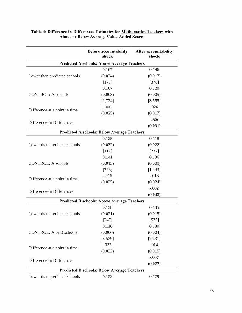
We observe this phenomenon more formally in the difference-in-difference analysis

presented in Table 4. As before, Table 4 compares mathematics teachers in schools that would

have received a given school grade in 2002 but for the policy change into schools that were

shocked downward to a lower grade and those that would have received the same school grade in

202 but were either unshocked or upward-shocked. This time, however, we further divide

teachers into those that were above-average and those that were below-average in terms of value

added for mathematics within the same type of schools (elementary, middle or high) for a

specific year. We see that above-average teachers in the pre-shock period were less likely to

leave schools downward-shocked to “F” than other would-be “D” schools, but in the post-shock

period they were considerable more likely to leave downward-shocked would-be “D” schools.

Moreover, the difference in difference is quite large: The difference post-shock versus pre-shock

is 13.2 percentage points, quite substantial when compared to the 21.2 percent pre-shock average

departure rate of above-average teachers in “D” schools. On the other hand, we see no significant

change after the shock versus before the shock in the likelihood that a below-average teacher

would leave a downward-shocked would-be “D” school versus an upward-shocked or unshocked

18

would-be “D” school (and the difference-in-difference coefficient is of the opposite sign of what

we observe vis-à-vis above-average teachers). We also find similar results if we use an

alternative time-varying measure of mathematics value-added, as seen in Appendix Table 3.12 In

summary, it appears that not only did the shock of downgrading a “D” school to an “F” grade

result in more teachers departing the school, it also resulted in the relatively high value-added

teachers disproportionately leaving the school.

C. Regression discontinuity estimates

The specific grading design of the Florida school accountability system implemented in

2002 facilitates the application of a regression discontinuity approach to obtain a local average

treatment effect of just barely receiving a grade of “F” as opposed to just barely missing the “F”

grade. As mentioned above, Florida’s 2002 grading system was based on a series of “grade

points” generated from the percentage of students meeting performance thresholds in reading,

writing and mathematics, the percentage of students making gains in reading and mathematics,

and the percentage of students in the bottom quartile of the school’s reading distribution making

gains in reading. In 2002, schools received grades of “A”, “B”, “C”, or “D”, respectively,

depending on whether they received at least 410, 380, 320, or 280 grade points out of 600

possible. Schools earning fewer than 280 grade points received a grade of “F” under the new

system. Because the state strictly adhered to its grading system13, the school grading system in

12 With regard to English/language arts (ELA) teachers, we tend to find that below-average teachers are somewhat more likely than are above-average teachers to leave schools shocked from “D” to “F”, though both groups are more likely to leave a predicted-“D” school that was downward-shocked. Results of the ELA analysis are available upon request. 13 A local mean smoothing plot of the probability of “F” grade receipt in 2002 and total school grading points earned in 2002 reveals a discrete jump from zero to one at the discontinuity of school grade points of 280. There was only one school with reported school grade points of 276 that was classified as "D" grade school. Only 55 teachers were affected by this potential misclassification. When we generated this school's grade using currently-available data, we calculated that the school actually should have received 282 points, suggesting that the initially-

19

Florida provides for a sharp discontinuity design (Imbens and Lemieux (2008)). The sharp RD

design identifies the causal effects of being an “F” school by comparing the teacher turnover

outcomes of the treatment and control groups with similar school grade points. A discrete jump

in the relationship between school grade points and teacher turnover in the neighborhood of the

cutoff is evidence of a causal impact of accountability pressure on teacher mobility. Due to the

uneven spacing of the cutoff points, schools with two neighboring letter grades are analyzed

together in our results. For example, we analyze the subsample of schools with a “D” or “F”

designation together. Altogether we have four analysis samples—“D” and “F” schools, “C” and

“D” schools, “B” and “C” schools, and “A” and “B” schools. In the following discussion we

focus on the subsample of “D” and “F” schools, though the same logic applies to the other three

subsamples.

As before, our outcome variable of interest is the probability of teacher turnover in the

year immediately following the policy change (Y , . The assignment variable Di,t is a

deterministic function of the forcing variable:

D , 1 x , (1a)

0 x , (1b)

where D indicates the treatment status of being an “F” school and indicates the known cutoff

of 280 grade points. If a school falls below the cutoff point of 280 in year 2002, the treatment

status Di takes a value of one.

The RD design mimics random assignment if teachers near the cutoff point have nearly

an identical chance of being treated, with just a random error determining whether at teacher’s

school falls above or below the school-grade threshold. The conditions for identification appear

reported school data were in error and later updated. (The state offered the opportunity for schools to challenge school grades.) We rely on the state's official grade points reports from 2002 for our analysis.

20

to hold in our case. As mentioned above, the details of the new accountability rules were not

announced until late in spring 2002 and the likelihood of teachers endogenously sorting across

the cutoff points is thus minimized. We also check the identification assumptions by examining

the turnover rate in the years prior to the policy change. Turnover in years prior to the policy

change should be unrelated to the cutoff points, i.e., we should not see a discrete jump in

turnover. Following the specification check suggested by Lee (2008), we present graphical

evidence of the probability of turnover as a function of school grade points for both the period

prior to the policy change and after the policy shock.

Figure 3 presents local mean smoothing plots of the probability of turnover against the

school grade points received in year 2002, along with 95 percent confidence bands for each of

the four academic years that are part of our analysis. The top two panels of Figure 3 depict the

relationship between teacher turnover and school grade points in the period prior to the policy

shock (the transition from 1999-2000 to 2000-01 and the transition from 2000-01 to 2001-02)

while the bottom two panels illustrate the relationship in the post-shock period (the transition

from 2001-02 to 2002-03 and the transition from 2002-03 to 2003-04). Consistent with the

unanticipated nature of the accountability shock, there is no discrete change in mobility at the

future grade cutoff and the overlapping confidence bands indicate that the likelihood of teacher

job change is not significantly different for teachers in schools just above or just below the

school grade cutoff for the pre-shock transitions, and if anything, in the 1999-2000 to 2000-01

transition, it appears that there is modestly lower turnover on the “F” side of the would-be “D”-

“F” boundary. For the 2001-02 to 2002-03 transition, the pattern is very noisy right at the

discontinuity, but this may be because moving immediately after the announcement of school

grades may not be feasible for many teachers. But by the first post-shock period in which

21

teacher mobility would have been comparatively possible (the transition from 2002-03 to 2003-

04), the estimated effect of an “F” grade relative to a “D” grade is about 5-8 percentage points

higher teacher turnover – in the same ballpark as the 4.9 percentage point difference observed in

our difference-in-difference results. As before, the difference is strongly statistically significant,

as the confidence bands on the left of the cutoff are at least 3 percentage points above the

confidence bands on the right of cutoff.

In our RD analysis we employ both non-parametric and parametric methods. The

flexibility of non-parametric methods allows them to accommodate a variety of non-linear

relationships. However, they require large numbers of observations near the cut point and are

sensitive to the choice of the range of values above/below the cutpoint that are included in the

analysis or “bandwidth”. Estimates from parametric methods, on the other hand, can be sensitive

to the selection of a functional form. Thus no approach is necessarily superior and the two

should be viewed as complements (Lee and Lemieux, 2010).

Our non-parametric RD analysis employs local linear regression (Hahn, Todd, and van

der Klaauw, 2001; Porter, 2003; Ludwig and Miller, 2007). This approach fits a kernel weighted

linear regression for any teacher observations that fall into the interval around the cutoff with the

radius being the bandwidth h. Specifically, we estimate the following:

Y , α τ ∗ D , β ∗ x , c β ∗ D , ∗ x , c ϵ

wherec h x , c h (2)

The difference between the left and right limits of this regression at the cutoff of 280 will be the

estimated impact of being rated as an “F” school in 2002. The coefficient τ in equation (2)

measures the impact on teacher turnover of being rated an “F” school in 2002. Taking advantage

of the panel nature of our dataset, we also estimate the same local linear regression using data

22

prior to 2002. Estimates from this pre-policy shock period serve as a specification check on our

identification near the cutoff. We do not expect to see any discontinuity during the pre-shock

period between future “F” schools and future “D” schools.

For such a non-parametric analysis, the choice of bandwidth is important. The bandwidth

defines the weight assigned to each observation. As the bandwidth gets smaller, the observations

close to the cutoff receive more weight in the estimation. Following Imbens and Lemieux, we

estimate the model with a range of bandwidths, varying from just around the cutoff to 30 or 40

points away from the cutoff depending on the segments of the subsample.14 In Table 5 we

present a variety of non-parametric RD estimates using both the optimal bandwidths proposed by

Calonico, Cattaneo and Titiunik (2014, 2015) and by Imbens and Kalyanaraman (2012). We

observe that the estimated effects of receiving an “F” grade instead of a “D” on teacher mobility

differ depending on the choice of optimal bandwidth selected: Using the CCT optimal bandwidth

of 10.151 points, we estimate an increase in teacher turnover of 8.16 percentage points, roughly a

40 percent increase in the departure rate for teachers, while the estimated magnitude of the

effects of an “F” grade on teacher turnover doubles when we instead apply the IK optimal

bandwidth of 18.094 points. Effects of changes in other school grade distribution are mixed.

Receiving a “C” grade instead of a “B” is associated with a 3.5-3.6 percentage point higher rate

of teacher turnover. In contrast, we do not detect a difference in terms of teacher turnover at

either the “D” versus “C” threshold or at the “B” versus “A” threshold.15

14 The largest bandwidth we examined is 40 points away from the cutoff for the “D”-versus-“F” and “C”-versus-“D” subsamples. The largest bandwidth is 30 points away from the cutoff for the “B”-versus-“C” and “A”-versus-“B” subsamples. 15 Although the point estimates of the impact of a school grade reduction on teacher turnover vary along the school grade distribution, only the results for shifting from a “D” to an “F” are robust to increases in bandwidth. For all other subsamples, varying the bandwidth leads to a lack of statistical significance at the discontinuities other than “D” versus “F”. On the other hand, the “D” versus “F” results are quite robust to changes in bandwidth used. Even with a bandwidth of 40 points, the point estimate of the impact of moving from a “D” to an “F” is still a seven percentage point increase in the teacher turnover rate.

23

We also consider implementation of our RD analysis in a parametric framework, and

follow Lee and Lemieux’s (2010) advice regarding selection of different parametric functional

forms. The simplest specification is a linear relationship between the probability of turnover and

school grade points:

Y , α τ ∗ D , β ∗ x , c ϵ, (3)

where the subscript t indicates the policy shock years of 2001-02 or 2002-03, and the subscript

t+1 represents the teacher’s status in the subsequent academic year. The coefficient τ measures

the causal impact of being designated a lower grade school, say an “F” school in year 2002, on

the turnover rate of teachers from one year to the next.

To account for possible nonlinearities, we also estimate parametric specifications using

polynomial quadratic and cubic terms. In addition, we present results using flexible quadratic

and flexible cubic terms to allow the slope of these polynomial functions to change on both sides

of cutoff. For example, the flexible cubic functional form yields the following equation.

Y , α τ ∗ D , β ∗ x , c β ∗ D , ∗ x , c β ∗ x , c β ∗ x , c

β ∗ D , ∗ x , c β ∗ D , ∗ x , c ϵ (4)

The coefficient estimate of τ using the post-policy shock cross-sectional data provides the

parametric estimate of the regression discontinuity effect.16 As suggested by Lee and Lemieux

(2010) as a mechanism for increasing the likelihood of smoothness in the covariates around the

discontinuity, we estimate parametric RD models with controls for the teacher’s age, race,

gender, salaries, education, experience level, certification areas, and subject area specialty, as

well as working conditions including average classroom, school and district-level student

demographic and socio-economic characteristics such as average student achievement scores on

16 We also use three pre-policy intervention years to provide evidence on the identification. As in our other specifications, we do not detect any discontinuity when we use three pre-policy intervention years.

24

the math portion of the FCAT, average number of disciplinary incidents per student, portion of

African American students, portion of Hispanic students, portion of students receiving free or

reduced-price lunches, and school-level average FCAT math score gains. We also estimate

parametric RD models without controls in order to be more comparable to the non-parametric

RD model specifications.

Table 6 presents the estimated effect of receiving a lower grade in a neighboring-letter-

grade subsample for the post-policy shock period only. We estimate, with and without controls,

linear polynomial quadratic, polynomial cubic, flexible quadratic, and flexible cubic versions of

the model. Across the specifications, the results tell the same story as that seen in the other

empirical models – that teachers in schools graded “F” after the 2002 grading shock are more

likely to leave the school than are teachers in schools graded “D” post-shock. Echoing the non-

parametric results, we find that receiving an “F” grade leads to a between 4.2 and 9.8 percentage

point greater turnover than a “D” grade, depending on the specification. As before, estimates

from subsamples other than the D/F discontinuity do not yield any consistent pattern.

In addition to the traditional RD estimates using the cross-sectional post-policy-shock

datasets (τ), we also estimate a variant of equation (4) in the panel data setting, incorporating a

difference-in-differences strategy. Essentially, we include a series of fixed effects for the

treatment dummy variables and the school grade points in 2002. Including these fixed effects

achieves two purposes. One is to control for any time-invariant trend in teacher turnover for

schools that received an “F” grade in 2002. The other is to capture any pre-existing differences

between hypothetical “F” schools and hypothetical “D” schools prior to the policy shock.

For each of the five parametric specifications, we estimate a difference-in-difference RD

design featuring data pooled from two pre-policy periods (departures between 1999-00 and

25

2000-01 and those between 2000-01 and 2001-02 and two post-policy periods (departures

between 2001-02 and 2002-03 and those between 2002-03 and 2003-04) with the

aforementioned controls. Each regression is estimated with two different samples: the

subsample including the neighboring grade, say “D” and “F” schools, and the subsample

including the predicted higher grade, for example predicted “D” schools. Estimates from the

various parametric models over the two samples are presented in the top and bottom panels of

Table 7, which confirm the earlier finding that the most robust results are for those schools

shocked from “D” to “F”. Being assigned an “F” grade translates into an increase in teacher

turnover of 3.5 to 9.5 percentage points, depending on the functional form. There is also

occasional, though less robust, evidence that a reduction in the school grade lessens turnover at

the upper end of the school grading scale. In the specifications without interaction terms,

schools receiving a “B” grade have turnover rates about one percentage point lower than “A”

schools, suggesting that there is on-the-job stress related to living up to the “A” standard.

The bottom panel of Table 7 provides evidence on the teachers’ responses to deviations

from the rating that their school would have received absent a change in the grading system.

Estimates are produced from sub-samples in which only schools that would have received an

equal grade or one letter grade higher (based on the old grading system) than they actually

received (based on the new grading system) are included in the analysis. As before, for example,

the “Predicted D” subsample includes schools that would have received a “D” under the old

system but earned an “F” or “D” under the new system; schools predicted to receive a “C” grade

or “F” grade under the old grading system are excluded. Teachers and administrators in some of

these “predicted to be D” schools were potentially in for a considerable surprise in Summer 2002

when they learned that instead of a “D” grade, their school will joining the ranks of “F” schools

26

– a designation that no schools in the state of Florida received in the preceding year. At the same

time, there are other “predicted to be D” schools which just missed the receipt of an “F” grade.

This near miss group should be nearly identical to the shocked-to-F grade schools. The estimated

impact of moving from a “D” to an “F” on teacher turnover from this closely matched subsample

is about four percentage points.

D. Regression discontinuity analysis by teacher quality

We next separate mathematics teachers based on whether they are above or below the

median in terms of value added, and estimate parametric RD and difference-in-difference RD

models using a variety of functional form assumptions; we present these results in Table 8. As

with the previous difference-in-difference and graphical evidence, we find that above-median

math teachers have close to a ten percentage point (or greater) higher turnover rate if their

schools are assigned an “F” grade instead of “D”, depending on the model specification.

Therefore, this analysis presents additional evidence to suggest that the principal effects of the

school grading system on teacher turnover involve the high-value-added teachers in schools that

were shocked downward from “D” to “F”.

V. Summary and Conclusions

This paper provides new evidence of the effects of school accountability systems on

teacher mobility. While prior papers on the subject analyzed the introduction of an accountability

system within a state, and therefore had no natural counterfactual, this study is the first to exploit

policy variation within the same state to study the effects of accountability on teacher job

changes.

27

Taking advantage of exogenous changes in accountability pressure for schools and using

a regression discontinuity design, we find that schools receiving an “F” grade instead of a “D”

grade will experience an increase in the turnover rate of 8-17 percentage points from the non-

parametric specification and roughly five percentage points from the parametric specification. In

addition to the traditional regression discontinuity estimate, we utilized the panel nature of the

data to derive regression discontinuity estimates enhanced by difference-in-differences. With

additional student, teacher, school and district controls, we find that missing a “D” grade

translates into 4-7 percentage points higher turnover rates. This increase in turnover reflects

primarily movement of teachers to other schools in the same district, but there is also significant

exit from public school teaching when schools are marked with a failing grade.

The mobility caused by school accountability also has significant effects on the

distribution of teacher quality within and across schools. We find that teachers with higher

value-added, as measured by contribution to test scores, are more likely to leave schools that

receive an “F” grade whereas the probability of departure for lower-rated teachers is unaffected.

This means that failing schools suffer a net reduction in average teacher quality. Those teachers

who stay may become more productive as a result of enhancing professional development

opportunities or increases in complementary inputs, such as reading coaches or funding for

increased remediation or a longer school day, that typically are provided to schools that fall into

the failing category in Florida.

The results have strong implications for public policy. Struggling schools that come

under increased accountability pressure face many challenges in terms of changing instructional

policies and practices to facilitate student improvement. We have discovered that (in the case of

those facing the highest accountability pressure) they also face the challenge of having to replace

28

more teachers, and particularly, their higher-quality teachers (measured in terms of contribution

to value-added). While a school accountability system can improve student outcomes, “failing”

schools face the challenge of holding on to their best teachers. It is noteworthy that the causal

evidence on school accountability indicates that schools identified as "failing" improved

following the school grading even as they were losing a disproportionate number of their best

teachers. The findings presented in this paper suggest that if these schools were able to retain

more of their high-quality teachers (perhaps through increased incentives to remain in the

school), the accountability gains could be greater still. On the other hand, these results suggest

that if schools lose a large number of their best teachers, the short-run gains associated with

school accountability pressure might be counteracted in the medium-run by differential

departures of high quality teachers. The interaction between effort responses and short-to-

medium-run teacher mobility as a consequence of accountability is a subject for further research.

29

References

Aaronson, Daniel, Lisa Barrow, and William Sander (2007). “Teachers and Student Achievement in the Chicago Public High Schools,” Journal of Labor Economics 25(1): 95–135.

Ballou, Dale and Matthew Springer (2008). "Achievement Tradeoffs and No Child Left Behind."

Working paper, Urban Institute.

Booher-Jennings, Jennifer (2005). "Below the Bubble: 'Educational Triage' and the Texas Accountability System." American Educational Research Journal 42: 231-268.

Boyd, Donald, Hamilton Lankford, Susanna Loeb, and James Wyckoff (2005). “Explaining the Short Careers of High-Achieving Teachers in Schools with Low-Performing Students,” American Economic Review 95(2): 166-171.

Boyd, Donald, Hamilton Lankford, Susanna Loeb, and James Wyckoff (2008). “The Impact of Assessment and Accountability on Teacher Recruitment and Retention: Are There Unintended Consequences?” Public Finance Review 36(1): 88-111.

Boyd, Donald, Hamilton Lankford, Pamela Grossman, Susanna Loeb, and James Wyckoff (2006). “How Changes in Entry Requirements Alter the Teacher Workforce and Affect Student Achievement,” Education Finance and Policy 1(2): 176-216.

Calonico, S., Cattaneo, M. D., & Titiunik, R. (2015). “Optimal data-driven regression discontinuity plots,” Journal of the American Statistical Association.

Calonico, S., Cattaneo, M. D., & Titiunik, R. (2014). “Robust data-driven inference in the regression-discontinuity design,” Stata Journal 14(4), 909-946.

Carnoy, Martin and Susanna Loeb (2002). “Does External Accountability Affect Student Outcomes? A Cross State Analysis,” Education Evaluation and Policy Analysis 24(4): 305-331.

Chakrabarti, Rajashri (2007). “Vouchers, Public School Response and the Role of Incentives: Evidence from Florida,” Staff Report No. 306, Federal Reserve Bank of New York.

Chiang, Hanley (2009). "How Accountability Pressure on Failing schools Affects Student Achievement," Journal of Public Economics, 93(9-10): 1045-1057.

Clotfelter, Charles, Helen Ladd, Jacob Vigdor, and Roger Aliaga Diaz (2004). “Do School Accountability Systems Make It More Difficult for Low Performing Schools to Attract and Retain High Quality Teacher?” Journal of Policy Analysis and Management 23(2): 251-271.

30

Craig, Steven, Scott Imberman, and Adam Perdue (2013). “Does it Pay to Get an A? School Resource Allocations in Response to Accountability Ratings,” Journal of Urban Economics.

Cullen, Julie Berry and Randall Reback (2007). “Tinkering Toward Accolades: School Gaming Under a Performance Accountability System,” In: Gronberg, Timothy J., Jansen, Dennis W. (Eds.), Advances in Applied Microeconomics 14 (Improving School Accountability), Elsevier.

Dee, Thomas and Brian Jacob (2011). "The Impact of No Child Left Behind on Student Achievement." Journal of Policy Analysis and Management.

Feng, Li (2009). “Opportunity Wages, Classroom Characteristics, and Teacher Mobility,” Southern Economic Journal 75(4), 1165-1190.

Feng, Li (2010). “Hire Today, Gone Tomorrow: New Teacher Classroom Assignments and Teacher Mobility,” Education Finance and Policy 5(3).

Feng, Li and Tim R. Sass (2011). “Teacher Quality and Teacher Mobility,” working paper, Florida State University. Working Paper #57. Washington DC: National Center for Analysis of Longitudinal Data in Education Research.

Figlio, David (2006). “Testing, Crime and Punishment,” Journal of Public Economics 90(4): 837-851.

Figlio, David and Lawrence Getzler (2007). “Accountability, Ability and Disability: Gaming the System?” In: Gronberg, Timothy J., Jensen, Dennis W. (Eds.), Advances in Applied Microeconomics vol. 14 (Improving School Accountability), Elsevier.

Figlio, David and Lawrence Kenny (2009). "Public Sector Performance Measurement and Stakeholder Support," Journal of Public Economics 93(9-10): 1069-1077.

Figlio, David and Maurice Lucas (2004). “What’s in a Grade? School Report Cards and the Housing Market,” American Economic Review 94(3): 591-604.

Figlio, David and Cecilia Rouse (2006). “Do Accountability and Voucher Threats Improve Low-Performing Schools?” Journal of Public Economics 90(1-2): 239-255.

Figlio, David and Joshua Winicki (2005). “Food for Thought? The Effects of School Accountability Plans on School Nutrition,” Journal of Public Economics 89(2-3): 381-394.

31

Goldhaber, Dan, Bethany Gross, and Daniel Player (2007). “Are Public Schools Really Losing Their “Best”? Assessing the Career Transitions of Teachers and Their Implications for the Quality of the Teacher Workforce.” Working Paper #12. Washington DC: National Center for Analysis of Longitudinal Data in Education Research.

Goldhaber, Dan and Jane Hannaway (2004). “Accountability with a Kicker: Preliminary

Observations on the Florida A+ Accountability Plan,” Phi Delta Kappan 85(8): 598-605.

Guarino, Cassandra, Mark Rckase, and Jeffrey Wooldridge (2012) Can Value-Added Measures of Teacher Education Performance be Trusted. Working Paper #18. The Education Policy Center at Michigan State University.

Hahn, Jinyong, Petra Todd, and Wilbert van der Klaauw (2001). “Identification and Estimation of Treatment Effects with a Regression-Discontinuity Design.” Econometrica, 69(1): 201–09.

Hanushek, Eric, John Kain, and Steven Rivkin (2004). “Why Public Schools Lose Teachers,” Journal of Human Resources 39(2): 326-354.

Hanushek, Eric and Margaret Raymond (2005). “Does School Accountability Lead to Improved Student Performance?” Journal of Policy Analysis and Management 24(2): 297-327.

Harris, Douglas N., Tim R. Sass and Anastasia Semykina (2011). “Value-Added Models and the Measurement of Teacher Productivity,” Working Paper #54. Washington DC: National Center for Analysis of Longitudinal Data in Education Research.

Imazeki, Jennifer (2005). “Teacher Salaries and Teacher Attrition,” Economics of Education Review 24(4): 431-449.

Imbens, G., & Kalyanaraman, K. (2011). “Optimal bandwidth choice for the regression discontinuity estimator,” Review of Economic Studies.

Imbens, Guido W., and Thomas Lemieux (2008). “Regression Discontinuity Designs: A Guide to Practice.” Journal of Econometrics 142(2): 615–35.

Jacob, Brian (2005). “Accountability, Incentives and Behavior: The Impact of High-Stakes Testing in the Chicago Public Schools,” Journal of Public Economics 89(5-6): 761-796.

Jacob, Brian and Steven Levitt (2003). “Rotten Apples: An Investigation of the Prevalance and Predictors of Teacher Cheating,” Quarterly Journal of Economics 118(3): 843-877.

Jackson, C. Kirabo (2012). “School Competition and Teacher Labor Markets: Evidence from Charter School Entry in North Carolina,” Journal of Public Economics 96(5-6): 431-438.

Jackson, C. Kirabo (2013). “Match Quality, Worker Productivity, and Worker Mobility: Direct Evidence from Teachers,” Review of Economics and Statistics.

32

Krieg, John (2006). “Teacher Quality and Attrition,” Economics of Education Review 25(1): 13-27.

Krieg, John (2008). “Are Students Left Behind? The Distributional Effects of the No Child Left Behind Act,” Education Finance and Policy 3(2): 250-281.

Ladd, Helen and Douglas Lauen (2009). "Status Versus Growth: The Distributional Effects of School Accountability Policies." Working paper, Urban Institute.

Lee, David S. (2008). “Randomized Experiments from Non-random Selection in U.S. House Elections.” Journal of Econometrics 142(2): 675–97.

Lee, David S. and Thomas Lemieux (2010). "Regression Discontinuity Designs in Economics," Journal of Economic Literature 48(2): 281-355.

Ludwig, Jens, and Douglas L. Miller (2007). “Does Head Start Improve Children’s Life Chances? Evidence from a Regression Discontinuity Design.” Quarterly Journal of Economics, 122(1): 159–208.

Neal, Derek and Diane Whitmore Schanzenbach (2010). “Left Behind by Design: Proficiency Counts and Test-Based Accountability,” Review of Economics and Statistics 92(2): 263-283.

Ozek, Umut (2010). "One Day Too Late? Mobile Students in an Era of Accountability." Working paper, Urban Institute.

Porter, Jack (2003). “Estimation in the Regression Discontinuity Model.” Unpublished manuscript.

Podgursky, Michael, Ryan Monroe and Donald Watson (2004). “The Academic Quality of Public School Teachers: An Analysis of Entry and Exit Behavior,” Economics of Education Review 23(5): 507-518.

Reback, Randall (2008). "Teaching to the Rating: School Accountability and the Distribution of Student Achievement," Journal of Public Economics 92(5-6): 1394-1415.

Reback, Randall, Jonah Rockoff and Heather Schwartz (2011). "Under Pressure: Job Security, Resource Allocation, and Productivity in Schools under NCLB." Working paper, Columbia University.

Rockoff, Jonah and Lesley Turner (2010). "Short-run Impacts of Accountability on School Quality." American Economic Journal: Economic Policy 2(4): 119-147.

33

Rouse, Cecilia, Jane Hannaway, Dan Goldhaber and David Figlio (2013). “Feeling the Florida Heat? How Low-Performing Schools Respond to Voucher and Accountability Pressure,”American Economic Journal: Economic Policy.

Scafidi, Benjamin, David Sjoquist, and Todd Stinebrickner (2007). “Race, Poverty and Teacher Mobility,” Economics of Education Review 26(2): 145-159.

West, Martin and Paul Peterson (2006). “The Efficacy of Choice Threats Within School Accountability Systems: Results from Legislatively Induced Experiments,” Economic Journal 116(510): C46-C62.

Wong, Manyee, Thomas Cook and Peter Steiner (2010). "No Child Left Behind: An Interim Evaluation of its Effects on Learning using two Interrupted Time Series Each with its Own Non-Equivalent Comparison Series." Working paper, Northwestern University.

34

Table 1: Number of Teachers and Schools by School Grade in Each Year

School Grade

Summer 1999

Summer 2000

Summer 2001

Summer 2002

Summer 2003

Summer 2004

A 8730 22285 27208 41384 56618 53094 (182) (548) (569) (885) (1234) (1256)

B 12913 1508 16664 26798 28996 25319 (298) (255) (396) (547) (560) (535)

C 62841 60601 57235 38027 29833 30795 (1176) (1108) (1067) (720) (529) (601)

D 24944 17411 13306 8685 7873 10267 (552) (357) (280) (175) (127) (174)

F 2805 128 0 2869 893 1455 (68) (4) (0) (56) (18) (32)

Total 112233 101933 114413 117763 124213 120930 (2276) (2272) (2312) (2383) (2468) (2598)

Source: Authors' calculations from state data. Number of teachers is presented first and number of schools is in parentheses.

35

Table 2: Comparison of Simulated and Actual School Grades in 2002

Actual Grade in 2002 based on new (summer 2002) grading system

A B C D F Row

Totals

Simulated grade in

2002 based on (summer

2001) grading system

A

11068 1203 0 0 0 12271

(284) (33) (0) (0) (0) (317)

B

2135 10148 2545 9 0 14837

(390) (209) (61) (1) (0) (661)

C

8765 15274 31461 3758 198 59456

(206) (301) (567) (68) (3) (1145)

D

212 139 3933 4824 2502 11610

(4) (3) (91) (102) (48) (248)

F 0 0 0 44 169 213

(0) (0) (0) (2) (5) (7)

Column Totals

22180 26764 37939 8635 2869 (884) (546) (719) (173) (56)

Note: Number of teachers is presented first and number of schools is in parentheses. Simulated grade changes are generated by applying both the old grading system and the new grading system to 2002 student test scores, using the approach introduced by Rouse et al. (2013). They are therefore generated based on precisely the same student tests; the only differences in calculations are the formulas used to convert these same tests into school grades.

36

Table 3: Difference-in-Differences Estimates of the Impact of Accountability Shock on Fraction of Teachers Leaving School

Before accountability

shock After accountability

shock

Predicted A schools

Lower than predicted schools

0.135 0.133

(0.007) (0.007)

[2,429] [2,439]

CONTROL: A schools

0.146 0.132

(0.002) (0.002)

[21,824] [22,205]

Difference at a point in time -0.011 0.001

(0.007) (0.007)

Difference-in Differences 0.012

(0.010)

Predicted B schools


0.168 0.173

(0.005) (0.005)

[5,000] [5,130]

CONTROL: A or B schools

0.156 0.153

(0.001) (0.001)

[60,065] [62,513]

Difference at a point in time 0.012* 0.020***

(0.005) (0.005)

Difference-in Differences 0.008

(0.007)

Predicted C schools


0.194 0.182

(0.004) (0.004)

[7,373] [7,812]

CONTROL: C or better schools

0.170 0.167

(0.001) (0.001)

[108,801] [110,807]

Difference at a point in time 0.024*** 0.015***

(0.005) (0.004)

Difference-in Differences -0.009

(0.006)

Predicted D schools

Lower than predicted schools 0.213 0.265

37

(0.006) (0.006)

[5,072] [5,036]

CONTROL: D or better schools

0.207 0.210

(0.003) (0.003)

[18,345] [18,263]

Difference at a point in time 0.006 .055***

(0.007) (0.007)

Difference-in Differences .049***

(0.009)

Note: Authors’ calculations from state data. Pre-shock periods refer to academic years 1999-2000 and 2000-01. Teacher departure status was derived based on information in year t and following year t+1. Teacher transitions between 1999-2000 and 2000-01 or between 2000-01 and 2001-02 are both counted as pre-shock movements. Post-shock periods refer to academic years 2001-02 and 2002-03. Teacher departure status was derived based on information in year t and following year t+1. Teacher transitions between 2001-02 and 2002-03 and 2002-03 are both counted as post-shock movements. The fraction of teachers who left school is listed for each group. Standard errors clustered at the school-by-year level are given in the parentheses; sample sizes are given in square brackets; ***p<0.001, **p<0.01, *p<0.05, #p<0.10.

38

Table 4: Difference-in-Differences Estimates for Mathematics Teachers with Above or Below Average Value-Added Scores



shock

Predicted A schools: Above Average Teachers


0.107 0.146

(0.024) (0.017)

[177] [378]

CONTROL: A schools

0.107 0.120

(0.008) (0.005)

[1,724] [3,555]

Difference at a point in time .000 .026

(0.025) (0.017)

Difference-in Differences .026

(0.031)

Predicted A schools: Below Average Teachers


0.125 0.118

(0.032) (0.022)

[112] [237]

CONTROL: A schools

0.141 0.136

(0.013) (0.009)

[723] [1,443]

Difference at a point in time -.016 -.018

(0.035) (0.024)

Difference-in Differences -.002

(0.042)

Predicted B schools: Above Average Teachers


0.138 0.145

(0.021) (0.015)

[247] [525]


0.116 0.130

(0.006) (0.004)

[3,529] [7,431]


(0.022) (0.015)


(0.027)

Predicted B schools: Below Average Teachers


39

(0.008) (0.017)

[209] [459]


0.153 0.159

(0.025) (0.006)

[2,035] [4,331]

Difference at a point in time -0.000 .020

(0.270) (0.018)


(0.032)

Predicted C schools: Above Average Teachers


0.178 0.144

(0.022) (0.015)

[259] [583]


0.145 0.149

(0.005) (0.004)

[4,884] [10,275]

Difference at a point in time .032 -.005

(0.023) (0.015)


(0.027)

Predicted C schools: Below Average Teachers


0.174 0.205

(0.022) (0.015)

[276] [624]


0.149 0.157

(0.006) (0.004)

[4,158] [9,468]

Difference at a point in time .025 .048***

(0.023) (0.015)


(0.027)

Predicted D schools: Above Average Teachers


0.129 0.254

(0.035) (0.022)

[132] [335]


0.212 0.206

(0.015) (0.011)

[697] [1,396]

Difference at a point in time -.084* .048#

(0.039) (0.025)

40

Difference-in Differences .132**

(0.046)

Predicted D schools: Below Average Teachers


0.266 0.254

(0.029) (0.021)

[192] [346]


0.169 0.188

(0.014) (0.009)

[829] [1,868]

Difference at a point in time .097** .066**

(0.032) (0.023)


(0.039)

Note: See Table 3; ***p<0.001, **p<0.01, *p<0.05, # p<0.10.

41

Table 5. Non-parametric Regression Discontinuity Estimates of the Effect of Receiving a Lower Grade on Teacher Turnover After the Policy Change

Subsample Indicators CCT Optimal

Bandwidth

IK Optimal Bandwidth

F versus D

Conventional 0.0718** 0.0273

Robust 0.0816** 0.167***

Conventional Std. Error (0.025) (0.020)

Teacher-year Observations [6586] [10312]

Bandwidth 10.151 18.094

D versus C

Conventional -0.00885 -0.00887

Robust -0.00794 0.00903



Bandwidth 14.133 14.653

C versus B

Conventional 0.0283* 0.0297*

Robust 0.0362* 0.0348*



Bandwidth 7.952 7.385

B versus A Conventional -0.0123 -0.0127

Robust -0.0127 -0.0133



Bandwidth 10.025 10.494

Note: Nonparametric local polynomial estimation is implemented using the robust bias-corrected confidence intervals proposed by Calonico, Cattaneo, Titiunik (2014). Average treatment-effects estimation from the CCT bandwidth is presented in Column (1) and similar estimation from Imbens and Kalyanaraman (2012) is presented in Column (2). Conventional estimates are presented first and followed by robust estimates. Standard errors are given in the parentheses; sample sizes are given in square brackets; ***p<0.001, **p<0.01, *p<0.05, #p<0.10.

42

Table 6. Parametric Regression Discontinuity Estimates of the Effect of Receiving a Lower Grade on Teacher Turnover After the Policy Change

Subsample Parametric Result(No Controls) Parametric Result (With Controls)

Linear Polynomial Quadratic

Polynomial Cubic

Flexible Quadratic

Flexible Cubic


Polynomial Cubic

Flexible Quadratic

Flexible Cubic

F versus D

0.0421# 0.0421# 0.0459 0.0584# 0.074 0.0583* 0.0529* 0.0594# 0.0718* 0.0976*

(0.023) (0.023) (0.032) (0.035) (0.051) (0.024) (0.026) (0.031) (0.034) (0.046)

[24762] [24762] [24762] [24762] [24762] [12503] [12503] [12503] [12503] [12503]

D versus C

0.0032 0.0056 0.0046 -0.0143 -0.0047 0.0061 0.0171 0.0167 0.0038 -0.0017

(0.009) (0.011) (0.011) (0.014) (0.018) (0.009) (0.011) (0.012) (0.014) (0.018)

[92843] [92843] [92843] [92843] [92843] [49829] [49829] [49829] [49829] [49829]

C versus B

0.0042 0.0034 0.0044 0.0116 0.0048 0.0117# 0.0104 0.0106 0.0095 -0.0005

(0.006) (0.007) (0.008) (0.010) (0.012) (0.007) (0.008) (0.008) (0.010) (0.013)

[126738] [126738] [126738] [126738] [126738] [68574] [68574] [68574] [68574] [68574]

B versus A

0.0056 0.0074 0.007 -0.0033 -0.0118 0.0075 0.0102 0.0093 0.0093 0.0098

(0.005) (0.007) (0.007) (0.010) (0.014) (0.006) (0.008) (0.008) (0.011) (0.014)

[135917] [135917] [135917] [135917] [135917] [71685] [71685] [71685] [71685] [71685]

Note: Each cell presents a separate estimate of the effect of the discontinuity on the probability of teacher mobility. Columns (1) to (5) display results from parametric models using linear, quadratic, cubic term in 2002 school points with last two models allowing for different slopes on both sides of cutoff. ***p<0.001, **p<0.01, *p<0.05, #p<0.10.

43

Table 7. Parametric Results for Neighboring Grade Subsamples and Predicted Higher Grade Samples Using Regression Discontinuity and Difference-In-Differences Method

A. Neighboring Grade Sample

Subsample Parametric Result(No Controls) Parametric Result(With Controls)


Polynomial Cubic

Flexible Quadratic

Flexible Cubic


Polynomial Cubic

Flexible Quadratic

Flexible Cubic

F versus D

0.0469* 0.0368# 0.0348 0.0573# 0.1010# 0.0523* 0.0331 0.037 0.0721# 0.0948

(0.017) (0.019) (0.022) (0.034) (0.053) (0.021) (0.027) (0.028) (0.043) (0.059)

[49080] [49080] [49080] [49080] [49080] [20146] [20146] [20146] [20146] [20146]

D versus C

-0.0045 -0.001 0.0012 0.0025 0.0052 -0.0083 0.0002 0.007 -0.0021 -0.016

(0.008) (0.010) (0.011) (0.019) (0.024) (0.009) (0.012) (0.012) (0.021) (0.025)

[184496] [184496] [184496] [184496] [184496] [80004] [80004] [80004] [80004] [80004]

C versus B

-0.0016 -0.0024 -0.0031 -0.0014 -0.0008 -0.0117# -0.0114# -0.0097 -0.0037 -0.0109

(0.005) (0.005) (0.007) (0.009) (0.013) (0.007) (0.007) (0.008) (0.011) (0.015)

[251391] [251391] [251391] [251391] [251391] [108469] [108469] [108469] [108469] [108469]

B versus A

-0.0024 -0.0031 0.0013 0.01 0.0005 -0.0115* -0.0132# -0.0112 0.0041 0.0141

(0.004) (0.005) (0.006) (0.013) (0.018) (0.005) (0.007) (0.008) (0.015) (0.021)

[267717] [267717] [267717] [267717] [267717] [107193] [107193] [107193] [107193] [107193]

B. Estimated Effect of Receiving a Lower-than-Expected Grade: Sample of Schools That Would Have Received a Higher Grade Under the Old Grading System



Polynomial Cubic

Flexible Quadratic

Flexible Cubic


Polynomial Cubic

Flexible Quadratic

Flexible Cubic

F versus D 0.0488* 0.0460* 0.0396* 0.033 0.0756 0.0465* 0.0445* 0.0236 0.0329 0.0555

(0.018) (0.018) (0.019) (0.032) (0.049) (0.021) (0.020) (0.023) (0.037) (0.048)

44

[46716] [46716] [46716] [46716] [46716] [16614] [16614] [16614] [16614] [16614]

D versus C

-0.0125 -0.0108 -0.0176 -0.0097 -0.0218 -0.013 -0.0113 -0.0188 0.0007 -0.0328

(0.011) (0.011) (0.013) (0.021) (0.025) (0.012) (0.012) (0.013) (0.023) (0.026)

[234793] [234793] [234793] [234793] [234793] [102114] [102114] [102114] [102114] [102114]

C versus B

0.0048 0.0002 0.0027 0.0363 0.0750* -0.0225# -0.0341* -0.0249 0.0096 0.0455

(0.009) (0.010) (0.012) (0.025) (0.034) (0.013) (0.014) (0.016) (0.033) (0.046)

[132708] [132708] [132708] [132708] [132708] [59160] [59160] [59160] [59160] [59160]

B versus A

-0.0011 -0.0024 -0.0006 0.0072 0.0065 0.0167 0.0168 0.0096 0.0274 0.0261

(0.012) (0.012) (0.013) (0.016) (0.017) (0.022) (0.022) (0.023) (0.030) (0.032)

[48897] [48897] [48897] [48897] [48897] [14117] [14117] [14117] [14117] [14117]

Note: Estimated RD marginal effects are presented first, followed by robust standard errors clustered at the school year level in parentheses and p-values in square brackets. “Predicted D” schools refer to schools that were predicted to be “D” schools under the old grading system. Column (1) to (10) report parametric results with different order of polynomial terms and different interaction terms. Flexible specifications such as flexible quadratic and cubic include interaction terms of treatment dummy and polynomial terms of school grade points. Included controls are as follows: p-th order polynomial terms of school grade points in 2002, interaction terms with dummy treatment status, classroom, school and district level controls such as average student achievement scores (levels and gains) on FCAT math, average number of disciplinary incidents, portion of African American students, portion of Hispanic students, portion of students on free or reduced lunch program. Teacher controls include teacher’s age, age squared, gender, gender and age interaction term, indicators for minority teachers, professional certification, other subject areas certification such as reading, middle or high school math, subject areas taught in, education level and years of experience, and teacher’s salaries. ***p<0.001, **p<0.01, *p<0.05, #p<0.10.

45

Table 8. Heterogeneity Results for Above-Average and Below-Average Quality Math Teachers

A. Neighboring Grade Sample



Polynomial Cubic

Flexible Quadratic

Flexible Cubic


Polynomial Cubic

Flexible Quadratic

Flexible Cubic

Above-Average

0.0827# 0.0961# 0.0775 0.2171* 0.1945 0.0984# 0.1168# 0.1047 0.1707 0.1036

(0.046) (0.051) (0.056) (0.094) (0.132) -0.057 (0.066) (0.069) (0.109) (0.127)

[2541] [2541] [2541] [2541] [2541] [1680] [1680] [1680] [1680] [1680]

Below-Average

0.0112 0.0118 0.0202 -0.041 0.0764 -0.0074 -0.0334 0.0079 0.0392 -0.094

(0.041) (0.044) (0.052) (0.077) (0.126) -0.058 (0.070) (0.076) (0.149) (0.166)

[3166] [3166] [3166] [3166] [3166] [2019] [2019] [2019] [2019] [2019]

B. Estimated Effect of Receiving a Lower-than-Expected Grade: Sample of Schools That Would Have Received a Higher Grade Under the Old Grading System



Polynomial Cubic

Flexible Quadratic

Flexible Cubic


Polynomial Cubic

Flexible Quadratic

Flexible Cubic

Above-Average

0.1421* 0.1477* 0.1014# 0.2325* 0.198 0.1857* 0.2090* 0.1685* 0.1877 0.0608

(0.055) (0.055) (0.059) (0.117) (0.168) (0.065) (0.069) (0.078) (0.147) (0.154)

[2560] [2560] [2560] [2560] [2560] [1570] [1570] [1570] [1570] [1570]

Below-Average

-0.004 -0.0183 -0.0157 -0.0363 0.0726 -0.0832 -0.0926 -0.1532* -0.127 -0.1031

(0.044) (0.044) (0.046) (0.087) (0.124) (0.057) (0.061) (0.071) (0.145) (0.154)

[3235] [3235] [3235] [3235] [3235] [1942] [1942] [1942] [1942] [1942]

Note: See notes for Table 7. Estimated RD marginal effects are presented first, followed by robust standard errors clustered at the school year level in parentheses and p-values in square brackets. Each cell presents a separate estimate of the discontinuity. Teachers are classified by the teacher value-added estimates from equation (5). Teacher quality estimates are split into halves. Each teacher quality subsample will compare teachers within that subsample across the state of Florida in the same school level. Panel A focuses on the neighboring grade of “D” and “F” while Panel B presents results from predicted “D” sample. ***p<0.001, **p<0.01, *p<0.05, #p<0.10.

46

Figure 1: Pre and post-shock distribution of value added in forecast “D” schools that received “D” or better in 2002

47

Figure 2: Pre and post-shock distribution of value added in forecast “D” schools that received “F” in 2002

48

Figure 3: Basic regression discontinuity evidence by academic years 1999-2000 to 2003-04

Notes: Local mean smoothing of the probability of teacher turnover for schools with different letter grade and their 95% confidence intervals (grey shaded area) are plotted.

49

Appendix Table 1: Difference-in-Differences Estimates of the Impact of Downward Shock on Fraction of Teachers Leaving School



shock

Predicted A schools

Downward shocked predicted A schools

0.135 0.133

(0.007) (0.007)

[2,429] [2,439]

No accountability shocked schools

0.146 0.132

(0.002) (0.002)

[21,824] [22,205]

Difference at a point in time -0.011 .001

(0.007) (0.007)


(0.010)

Predicted B schools

Downward shocked predicted B schools

0.168 0.173

(0.005) (0.005)

[5,000] [5,130]


0.159 0.157

(0.003) (0.003)

[19,732] [20,197]

Difference at a point in time 0.009 .017**

(0.006) (0.006)


(0.008)

Predicted C schools

Downward shocked predicted C schools

0.194 0.182

(0.004) (0.004)

[7,373] [7,812]


0.177 0.175

(0.002) (0.002)

[61,962] [62,742]

Difference at a point in time 0.018*** .008

(0.005) (0.005)

Difference-in Differences -0.010

(0.007)

50

Predicted D schools

Downward shocked predicted D schools

0.213 0.265

(0.006) (0.006)

[5,072] [5,036]


0.204 0.216

(0.004) (0.004)

[9,605] [9,634]

Difference at a point in time 0.009 .050***

(0.007) (0.007)

Difference-in Differences .041***

(0.010)


51

Appendix Table 2: Difference-in-Differences Estimates of the Impact of Upward Shock on Fraction of Teachers Leaving School



shock

Predicted B schools

Upward shocked predicted B school

0.154 0.152

(0.002) (0.002)

[40,333] [42,316]


0.159 0.157

(0.003) (0.003)

[19,732] [20,197]

Difference at a point in time -0.005 -.005

(0.003) (0.003)


(0.004)

Predicted C schools

Upward shocked predicted C school

0.162 0.157

(0.002) (0.002)

[46,839] [48,065]


0.177 0.175 (0.002) (0.001)

[61,962] [62,742]

Difference at a point in time -0.015*** -.018***

(0.002) (0.002)


(0.003)

Predicted D schools

Upward shocked predicted D school

0.209 0.205

(0.004) (0.004)

[8,740] [8,629]


0.204 0.216

(0.004) (0.004)

[9,605] [9,634]

Difference at a point in time 0.006 -.011

(0.006) (0.006)


(0.009)

Predicted F schools

Upward shocked predicted F school

0.272 0.191

(0.046) (0.047)

52

[92] [89]


0.314 0.232

(0.024) (0.024)

[334] [332]

Difference at a point in time -0.043 -.041

(0.052) (0.053)


(0.074)


53

Appendix Table 3: Difference-in-Differences Estimates for Mathematics Teachers with Above or Below Average Value-Added Scores(Alternative

measure)



shock

Predicted A schools: Above Average Teachers


0.101 0.146

(0.027) (0.018)

[148] [335]

CONTROL: A schools

0.106 0.121

(0.009) (0.006)

[1,288] [2,703]

Difference at a point in time -.004 .025

(0.028) (0.019)


(0.034)

Predicted A schools: Below Average Teachers


0.128 0.121

(0.028) (0.020)

[141] [280]

CONTROL: A schools

0.130 0.128

(0.010) (0.007)

[1,159] [2,295]

Difference at a point in time -.003 -.006

(0.300) (0.021)


(0.037)

Predicted B schools: Above Average Teachers


0.136 0.150

(0.024) (0.016)

[198] [434]


0.116 0.132

(0.006) (0.004)

[2,999] [6,145]


(0.024) (0.017)


(0.030)

Predicted B schools: Below Average Teachers


54

(0.022) (0.015)

[258] [550]


0.145 0.151

(0.007) (0.005)

[2,565] [5,617]


(0.023) (0.016)


(0.028)

Predicted C schools: Above Average Teachers


0.187 0.165

(0.022) (0.014)

[268] [617]


0.145 0.147

(0.005) (0.004)

[4,380] [9,260]


(0.022) (0.015)


(0.027)

Predicted C schools: Below Average Teachers


0.165 0.186

(0.022) (0.015)

[267] [590]


0.149 0.158

(0.005) (0.004)

[4,662] [10,483]


(0.023) (0.015)


(0.028)

Predicted D schools: Above Average Teachers


0.155 0.252

(0.030) (0.019)

[174] [452]


0.188 0.201

(0.014) (0.010)

[805] [1,740]

Difference at a point in time -.032 .051*

(0.034) (0.021)

55

Difference-in Differences .083*

(0.040)

Predicted D schools: Below Average Teachers


0.273 0.258

(0.033) (0.026)

[150] [229]


0.190 0.189

(0.015) (0.010)

[721] [1,526]

Difference at a point in time .083* .068*

(0.036) (0.028)


(0.046)


Date post:	23-Jun-2018
Category:	Documents
Upload:	tranliem
View:	214 times
Download:	0 times

SCHOOL ACCOUNTABILITY AND TEACHER Mtsass/pdfs/feng figlio sass revised 20160624 jue... · 1 SCHOOL...

Documents