university-logo

ReviewParabolic PDEs

Summary

PARABOLIC PDES

Dr. Johnson

School of Mathematics

Semester 1 2008

Dr. Johnson MATH65241

university-logo

ReviewParabolic PDEs

Summary

OUTLINE

1 REVIEW

2 PARABOLIC PDES

ExamplesThe Heat EquationExplicit MethodImplicit Method

3 SUMMARY

Dr. Johnson MATH65241

university-logo

ReviewParabolic PDEs

Summary

OUTLINE

1 REVIEW

2 PARABOLIC PDES

ExamplesThe Heat EquationExplicit MethodImplicit Method

3 SUMMARY

Dr. Johnson MATH65241

university-logo

ReviewParabolic PDEs

Summary

OUTLINE

1 REVIEW

2 PARABOLIC PDES

ExamplesThe Heat EquationExplicit MethodImplicit Method

3 SUMMARY

Dr. Johnson MATH65241

university-logo

ReviewParabolic PDEs

Summary

ELLIPTIC PDES

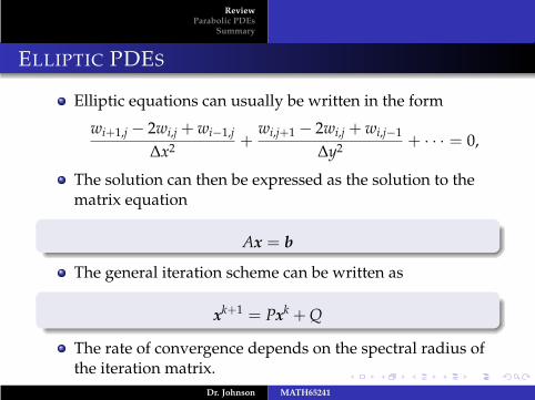
Elliptic equations can usually be written in the form

wi+1,j − 2wi,j +wi−1,j

∆x2+

wi,j+1 − 2wi,j +wi,j−1

∆y2+ · · · = 0,

The solution can then be expressed as the solution to thematrix equation

Ax = b

The general iteration scheme can be written as

xk+1 = Pxk +Q

The rate of convergence depends on the spectral radius ofthe iteration matrix.

Dr. Johnson MATH65241

university-logo

ReviewParabolic PDEs

Summary

ELLIPTIC PDES

Elliptic equations can usually be written in the form

wi+1,j − 2wi,j +wi−1,j

∆x2+

wi,j+1 − 2wi,j +wi,j−1

∆y2+ · · · = 0,

The solution can then be expressed as the solution to thematrix equation

Ax = b

The general iteration scheme can be written as

xk+1 = Pxk +Q

The rate of convergence depends on the spectral radius ofthe iteration matrix.

Dr. Johnson MATH65241

university-logo

ReviewParabolic PDEs

Summary

ExamplesThe Heat EquationExplicit MethodImplicit Method

OUTLINE

1 REVIEW

2 PARABOLIC PDES

ExamplesThe Heat EquationExplicit MethodImplicit Method

3 SUMMARY

Dr. Johnson MATH65241

university-logo

ReviewParabolic PDEs

Summary

ExamplesThe Heat EquationExplicit MethodImplicit Method

EXAMPLES

One of the simplest parabolic pde is the diffusion equationwhich in one space dimensions is

∂u

∂t= κ

∂2u

∂x2.

For two or more space dimensions we have

∂u

∂t= κ∇2u

In the above κ is some given constant.

Dr. Johnson MATH65241

university-logo

ReviewParabolic PDEs

Summary

ExamplesThe Heat EquationExplicit MethodImplicit Method

EXAMPLES

Another familiar set of parabolic pdes is the boundarylayer equations

ux + yy =0,

ut + uux + vuy = − px + uyy,

0 = − py.

Dr. Johnson MATH65241

university-logo

ReviewParabolic PDEs

Summary

ExamplesThe Heat EquationExplicit MethodImplicit Method

OUTLINE

1 REVIEW

2 PARABOLIC PDES

ExamplesThe Heat EquationExplicit MethodImplicit Method

3 SUMMARY

Dr. Johnson MATH65241

university-logo

ReviewParabolic PDEs

Summary

ExamplesThe Heat EquationExplicit MethodImplicit Method

INITIAL CONDITIONS

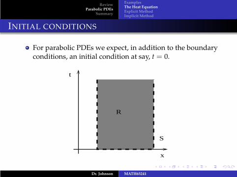
For parabolic PDEs we expect, in addition to the boundaryconditions, an initial condition at say, t = 0.

R

S

x

t

Dr. Johnson MATH65241

university-logo

ReviewParabolic PDEs

Summary

ExamplesThe Heat EquationExplicit MethodImplicit Method

HEAT EQUATION

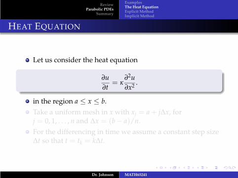
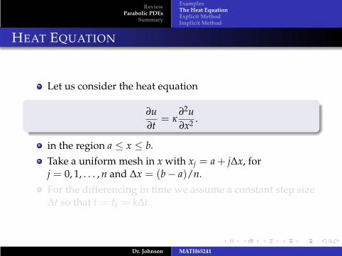
Let us consider the heat equation

∂u

∂t= κ

∂2u

∂x2.

in the region a ≤ x ≤ b.

Take a uniform mesh in xwith xj = a+ j∆x, forj = 0, 1, . . . ,n and ∆x = (b− a)/n.

For the differencing in time we assume a constant step size∆t so that t = tk = k∆t.

Dr. Johnson MATH65241

university-logo

ReviewParabolic PDEs

Summary

ExamplesThe Heat EquationExplicit MethodImplicit Method

HEAT EQUATION

Let us consider the heat equation

∂u

∂t= κ

∂2u

∂x2.

in the region a ≤ x ≤ b.

Take a uniform mesh in xwith xj = a+ j∆x, forj = 0, 1, . . . ,n and ∆x = (b− a)/n.

For the differencing in time we assume a constant step size∆t so that t = tk = k∆t.

Dr. Johnson MATH65241

university-logo

ReviewParabolic PDEs

Summary

ExamplesThe Heat EquationExplicit MethodImplicit Method

HEAT EQUATION

Let us consider the heat equation

∂u

∂t= κ

∂2u

∂x2.

in the region a ≤ x ≤ b.

Take a uniform mesh in xwith xj = a+ j∆x, forj = 0, 1, . . . ,n and ∆x = (b− a)/n.

For the differencing in time we assume a constant step size∆t so that t = tk = k∆t.

Dr. Johnson MATH65241

university-logo

ReviewParabolic PDEs

Summary

ExamplesThe Heat EquationExplicit MethodImplicit Method

OUTLINE

1 REVIEW

2 PARABOLIC PDES

ExamplesThe Heat EquationExplicit MethodImplicit Method

3 SUMMARY

Dr. Johnson MATH65241

university-logo

ReviewParabolic PDEs

Summary

ExamplesThe Heat EquationExplicit MethodImplicit Method

FIRST ORDER APPROXIMATION

We may approximate our equation by

wk+1j −wk

j

∆t= κ

[

wkj+1 − 2wk

j +wkj−1

∆x2

]

.

Here wkj denotes an approximation to the exact solution

u(x, t) of the pde at x = xj, t = tk.

The above scheme is first order in time O(∆t) and secondorder in space O(∆x)2.

This scheme is explicit because the unknowns at level k+ 1can be computed directly.

Dr. Johnson MATH65241

university-logo

ReviewParabolic PDEs

Summary

ExamplesThe Heat EquationExplicit MethodImplicit Method

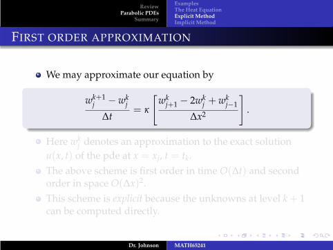
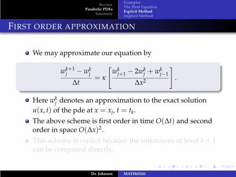
FIRST ORDER APPROXIMATION

We may approximate our equation by

wk+1j −wk

j

∆t= κ

[

wkj+1 − 2wk

j +wkj−1

∆x2

]

.

Here wkj denotes an approximation to the exact solution

u(x, t) of the pde at x = xj, t = tk.

The above scheme is first order in time O(∆t) and secondorder in space O(∆x)2.

This scheme is explicit because the unknowns at level k+ 1can be computed directly.

Dr. Johnson MATH65241

university-logo

ReviewParabolic PDEs

Summary

ExamplesThe Heat EquationExplicit MethodImplicit Method

FIRST ORDER APPROXIMATION

We may approximate our equation by

wk+1j −wk

j

∆t= κ

[

wkj+1 − 2wk

j +wkj−1

∆x2

]

.

Here wkj denotes an approximation to the exact solution

u(x, t) of the pde at x = xj, t = tk.

The above scheme is first order in time O(∆t) and secondorder in space O(∆x)2.

This scheme is explicit because the unknowns at level k+ 1can be computed directly.

Dr. Johnson MATH65241

university-logo

ReviewParabolic PDEs

Summary

ExamplesThe Heat EquationExplicit MethodImplicit Method

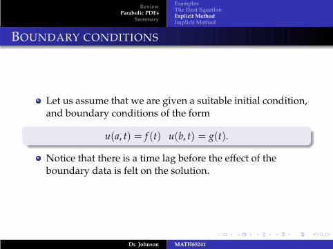
BOUNDARY CONDITIONS

Let us assume that we are given a suitable initial condition,and boundary conditions of the form

u(a, t) = f (t) u(b, t) = g(t).

Notice that there is a time lag before the effect of theboundary data is felt on the solution.

Dr. Johnson MATH65241

university-logo

ReviewParabolic PDEs

Summary

ExamplesThe Heat EquationExplicit MethodImplicit Method

STABILITY CONDITION

As we will see later this scheme is conditionally stable for

β ≤1

2

where

β =κ∆t

∆x2.

Note that β is sometimes called the Peclet or diffusionnumber.

Dr. Johnson MATH65241

university-logo

ReviewParabolic PDEs

Summary

ExamplesThe Heat EquationExplicit MethodImplicit Method

OUTLINE

1 REVIEW

2 PARABOLIC PDES

ExamplesThe Heat EquationExplicit MethodImplicit Method

3 SUMMARY

Dr. Johnson MATH65241

university-logo

ReviewParabolic PDEs

Summary

ExamplesThe Heat EquationExplicit MethodImplicit Method

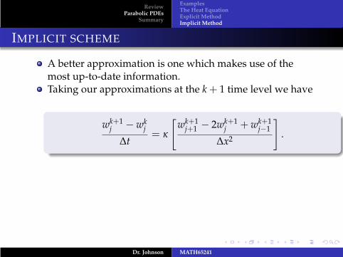
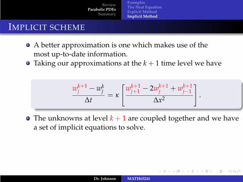
IMPLICIT SCHEME

A better approximation is one which makes use of themost up-to-date information.Taking our approximations at the k + 1 time level we have

wk+1j −wk

j

∆t= κ

[

wk+1j+1 − 2wk+1

j +wk+1j−1

∆x2

]

.

Dr. Johnson MATH65241

university-logo

ReviewParabolic PDEs

Summary

ExamplesThe Heat EquationExplicit MethodImplicit Method

IMPLICIT SCHEME

A better approximation is one which makes use of themost up-to-date information.Taking our approximations at the k + 1 time level we have

wk+1j −wk

j

∆t= κ

[

wk+1j+1 − 2wk+1

j +wk+1j−1

∆x2

]

.

The unknowns at level k + 1 are coupled together and we havea set of implicit equations to solve.

Dr. Johnson MATH65241

university-logo

ReviewParabolic PDEs

Summary

ExamplesThe Heat EquationExplicit MethodImplicit Method

SYSTEM OF EQUATIONS

Rearrange to get

−βwk+1j+1 + (1+ 2β)wk+1

j − βwk+1j−1 = wk

j ,

for 1 ≤ j ≤ n− 1

Approximation of the boundary conditions gives

wk+10 = f (tk+1), wk+1

n = g(tk+1)

We have a tridiagonal system of equations.

Dr. Johnson MATH65241

university-logo

ReviewParabolic PDEs

Summary

ExamplesThe Heat EquationExplicit MethodImplicit Method

SYSTEM OF EQUATIONS

Rearrange to get

−βwk+1j+1 + (1+ 2β)wk+1

j − βwk+1j−1 = wk

j ,

for 1 ≤ j ≤ n− 1

Approximation of the boundary conditions gives

wk+10 = f (tk+1), wk+1

n = g(tk+1)

We have a tridiagonal system of equations.

Dr. Johnson MATH65241

university-logo

ReviewParabolic PDEs

Summary

ExamplesThe Heat EquationExplicit MethodImplicit Method

PROPERTIES OF THE SCHEME

We can use direct methods to solve a tridiagonal system ofequations.

The scheme is only first order, the same as the explicitscheme.

However it is unconditionally stable - there are norestriction on the magnitude of β.

Dr. Johnson MATH65241

university-logo

ReviewParabolic PDEs

Summary

ExamplesThe Heat EquationExplicit MethodImplicit Method

PROPERTIES OF THE SCHEME

We can use direct methods to solve a tridiagonal system ofequations.

The scheme is only first order, the same as the explicitscheme.

However it is unconditionally stable - there are norestriction on the magnitude of β.

Dr. Johnson MATH65241

university-logo

ReviewParabolic PDEs

Summary

FIRST ORDER METHODS FOR PARABOLIC PDES

The explicit method is the simplest method, taking thedifference approximations at tk.

The scheme is first order in t,The stability condition requires β ≤ 1/2.

The implicit method takes the difference approximationsat tk+1

The scheme is first order in t,The scheme is unconditionally stable.

Like the modified Euler method for ODEs, we can take ourdifference equations at tk+1/2 to increase the order of thescheme.

Next time - second order schemes. . .

Dr. Johnson MATH65241

university-logo

ReviewParabolic PDEs

Summary

FIRST ORDER METHODS FOR PARABOLIC PDES

The explicit method is the simplest method, taking thedifference approximations at tk.

The scheme is first order in t,The stability condition requires β ≤ 1/2.

The implicit method takes the difference approximationsat tk+1

The scheme is first order in t,The scheme is unconditionally stable.

Like the modified Euler method for ODEs, we can take ourdifference equations at tk+1/2 to increase the order of thescheme.

Next time - second order schemes. . .

Dr. Johnson MATH65241

university-logo

ReviewParabolic PDEs

Summary

FIRST ORDER METHODS FOR PARABOLIC PDES

The explicit method is the simplest method, taking thedifference approximations at tk.

The scheme is first order in t,The stability condition requires β ≤ 1/2.

The implicit method takes the difference approximationsat tk+1

The scheme is first order in t,The scheme is unconditionally stable.

Like the modified Euler method for ODEs, we can take ourdifference equations at tk+1/2 to increase the order of thescheme.

Next time - second order schemes. . .

Dr. Johnson MATH65241