arX

iv:0

711.

4885

v3 [

astr

o-ph

] 1

1 Se

p 20

08

Galaxy redshift abundance periodicity from Fourier analysis of

number counts N(z) using SDSS and 2dF GRS galaxy surveys

J.G. HartnettSchool of Physics, the University of Western Australia

35 Stirling Hwy, Crawley 6009 WA Australia; john@physics.uwa.edu.au

K. HiranoDepartment of Physics, Tokyo University of Science

1-3 Kagurazaka Shinjuku-ku, Tokyo 162-8601, Japan; h-koichi@guitar.ocn.ne.jp

ABSTRACT

A Fourier analysis on galaxy number counts from redshift data of both the Sloan DigitalSky Survey and the 2dF Galaxy Redshift Survey indicates that galaxies have preferred periodicredshift spacings of ∆z = 0.0102, 0.0246, and 0.0448 in the SDSS and strong agreement withthe results from the 2dF GRS. The redshift spacings are confirmed by the mass density fluctua-tions, the power spectrum P (z) and Npairs calculations. Application of the Hubble law results ingalaxies preferentially located on co-moving concentric shells with periodic spacings. The com-bined results from both surveys indicate regular co-moving radial distance spacings of 31.7± 1.8h−1Mpc, 73.4± 5.8 h−1Mpc and 127± 21 h−1Mpc. The results are consistent with oscillationsin the expansion rate of the universe over past epochs.

Subject headings: galaxies:distances and redshifts—large-scale structure of universe

1. Introduction

When modeling the large scale structure ofthe cosmos the cosmological principle is assumed,therefore what we see must be biased by our view-point. The assumption is that the universe hasexpanded over time and any observer at any placeat the same epoch would see essentially the samepicture of the large scale distribution of galaxiesin the universe.

However evidence has emerged from both the2dF Galaxy Redshift Survey (2dF GRS) (see fig.17 of Colless et al (2001)) and also the Sloan Dig-ital Sky Survey (SDSS) (see fig. 2 of Tegmark etal (2004)) that seem to indicate that there is peri-odicity in the abundances of measured galaxy red-shifts. This has emerged from the galaxy numbercounts (N) within a small redshift interval (δz) asa function of redshift (z).

What has been found is the so-called picket-

fence structure of the N -z relation, first noticedin one dimension by Broadhurst et al (1990) froma pencil-beam survey of field galaxies. In this pa-per the galaxy surveys are analysed on 2D and3D scales. The usual interpretation is that thisis evidence of the Cosmic Web, including voidsand long filaments of galaxies. An alternative in-terpretation is suggested in this paper; galaxiesare preferentially found in redshift space at cer-tain redshifts with higher number densities thanat other redshifts. Of course, this does not ruleout cosmic web structures in addition to this ef-fect.

However the concept that this represents realspace galaxy distances is incompatible with thecosmological principle, which assumes the unifor-mity of space at all epochs on sufficiently largeenough scales. And it has been demonstrated(Yoshida et al 2001), from a large number of nu-merical simulations using the Einstein-de Sitter

1

and ΛCDM models, that the probability of get-ting such a periodic spatial structure from cluster-ing and Cosmic Web filaments is less than 10−3.This allows for an alternate explanation, namelythat the redshift periodicity is evidence for pastoscillations in the expansion rate of the universe.

The only information that has been sought fromlarge scale galaxy surveys is the spatial powerspectrum that describes the random yet uniformdistribution of galaxies in the universe, where theonly departure expected from the random distri-bution is some characteristic scale for the cluster-ing of galaxies. Certainly very few expect to findevidence consistent with a periodic redshift distri-bution.

However Hirano et al (2008) have attempted toexplain galaxy redshift abundance periodicity asa real effect resulting from the universe having anon-minimally coupled scalar field that manifests,in later cosmological times. The effect producedoscillations in the expansion rate as a function oftime. They model not only the redshift space ob-servations but also the effect their cosmology hason the CMB power spectrum and the type Ia su-pernova Hubble diagram.

In the usual analysis the spatial two-point orautocorrelation function is used to define the ex-cess probability, compared to that expected for arandom distribution, of finding a pair of galax-ies at a given separation (Baugh 2006). As aresult the power spectrum P (k) is derived fromthe two-point correlation function (Peebles 1980).The power spectrum is predicted by theories forthe formation of large scale structure in the uni-verse and compared with that measured, or moreprecisely calculated from the available data.

The power spectrum for the SDSS has beencalculated using a set of basis functions definedin (Hamilton et al. 2000). Three power spec-tra (galaxy-galaxy, galaxy-velocity, and velocity-velocity) were determined. Local motions ofgalaxies only contribute a radial component of agalaxy’s total redshift, hence only affect the radialcomponent of the power spectrum. Because theangular power spectrum is unaffected the assump-tion is also made that galaxy-galaxy spectrum isequal to the redshift-space power spectrum in thetransverse direction. In this paper we analyzethe redshift hence radial component of the powerspectrum P (z), calculated in redshift space not

k-space, and find periodicity consistent with thatobserved in N(z). Also an Npairs analysis is car-ried out on both survey data sets with confirmingresults.

The “Bull’s-eye” effect has been studied (Praton et al. 1997;Melott et al. 1998; Thomas et al 2004) via N -body simulations to result from large-scale in-fall plus small-scale virial motion of galaxies. Itis believed that these two effects can bias mea-surements of large scale real space galaxy dis-tributions. One is the so-called “fingers-of-God”(FOG) effect, which results from random peculiarmotions of galaxies at the same distance from theobserver. The second acts on much larger scalesand where overdensities of galaxies occur, like atthe “Great Wall” for instance. See Fig. 1.

Galaxies tend to have local motions towardthe center of such structures. These motions arenot random but coherent and add or subtractto the observer’s line-of-sight redshift determina-tion. These effects preferentially distort the mapin redshift space toward the observer due to thevelocities of galaxies within clusters, i.e. non-cosmological redshift contributions. However thelatter can only enhance in redshift space existingweak real space structures, it cannot create con-centric structures centered on the Galaxy. Andthe FOG effect tends to smooth out finer detailedor higher Fourier frequency structures in redshiftspace and is not very relevant to this discussion.

In the maps, fig. 18 of Colless et al (2001))and fig. 4 of Tegmark et al (2004), there appearsto the eye to be concentric structure in the ar-rangement of galaxies. See the left hand side ofthe Fig. 1, the SDSS data with declinations be-tween 0 and 6 mapped in Cartesian coordinates.Could it be that we inhabit a region of the Uni-verse that is a bubble, part of a background ofmany such bubbles? But because redshift onlygives us one dimensional information the conclu-sion could be drawn that if the galaxies in theUniverse are evenly distributed throughout thenredshift periodicity is indicative of oscillations inthe expansion at past epochs. All observers wouldsee the same shell structure in redshift space re-gardless of their location.

In this analysis we take a heuristic approachand look for periodicity in the redshift spacing be-tween galaxies, in 2D in the case of slices and in3D in case of the whole SDSS data set. In practice

2

the discrete Fourier Transform (νs) is calculatedfrom the N -z relations, which are histograms de-termined by binning (counting) the observed red-shifts of the survey galaxies between z− δz/2 andz + δz/2, as a function of redshift z. Within theith bin there are ∆Ni galaxies. Discrete Fourieramplitudes νs are generated for each integer s > 1from

νs =1√n

n∑

i=1

use2πj(i−1)(s−1)/n, (1)

where us = ∆Ni, j =√−1, n is the total number

of ∆Ni bins. Because νs are complex their abso-lute value is taken in the analysis. The Fourierfrequencies are calculated from

F =nδz

s= ∆z. (2)

where ∆z is the periodic redshift interval.

The results suggest that there are redshifts, onthe scale size discussed here, which is not primar-ily the result of clustering or the FOG and infalleffects resulting in distortion of the redshift spacemaps. Both the SDSS and 2dF GRS redshift datawhere the redshifts are known with 95% confidenceor greater are used. Fourier analysis can find pe-riodic structure even where it may not be so ap-parent to the eye.

Data for 427,513 galaxies from the SDSS FifthData Release (DR5) were obtained where the dataare primarily sampled from within about -10 to70 degrees of the celestial equator. Also data for229,193 galaxies were obtained from the 2dFGRSwhere the data are confined to within 2 degreesnear the celestial equator and balanced betweenthe Northern and Southern hemispheres. In theSDSS case the data are not so well balanced, yetthere are nearly twice as many usable data.

2. Fourier analysis of N-z relations

2.1. 2D slices of SDSS data

From the SDSS data three 6 slices were takenin declination (Dec) angle for examination andcomparison. They were taken from 0 < Dec < 6

, 40 < Dec < 46 and 52 < Dec < 58. A realspace Cartesian plot (with aspect ratio of unity)of the data from the first slice near the equato-rial plane is shown in Fig. 1. The redshifts have

been converted to co-moving radial distance withHubble constant H0 = 100 kms−1Mpc−1 wherethe parameter h = H0/100. The Great Wall isshown in the second and third quadrants as indi-cated. In those two quadrants it is evident to theeye that there is general concentric structure witha spacing of about 75 h−1Mpc.

Polar coordinate maps of these regions, pro-jected onto the equatorial plane, are shown in Figs2, 3 and 4, respectively. Most of the SDSS datacome from two declination bands on the sky. Thefirst slice is taken from the lower band near thecelestial equator and the latter two from higherdeclinations. Polar maps can tend to distort a realspace image but a comparison of Figs 1 and 2 in-dicates that these polar plots would be very closein appearance to real space maps if converted toco-moving coordinates.

From simple inspection concentric structure isapparent in both Figs 2 and 4 but not as apparentin Fig. 3. To the eye this seems too coinciden-tal and deserves further investigation. At least atsome declinations the case can be made for red-shift periodicity.

These data were binned with a bin size δz =10−3 resulting in a N -z relation. The redshift res-olution of most, but not all, of the SDSS datais only 10−3. This bin size essentially counts allgalaxies of the same redshift regardless of theirposition on the sky.

Using (1) the discrete Fourier spectra were cal-culated for N(z) of each data slice, and are shownin Fig. 5. The Fourier frequency axis in Fig. 5,and all subsequent figures, has been converted toa redshift interval (∆z). For the lowest angle slice(solid black curve) from the data of Fig. 2 andthe highest angle slice (solid gray curve) from thedata of Fig. 4 the peaks at numbers 1 and 2 co-incide. For the data from the 40 < Dec < 46

slice of Fig. 3 the peaks are not strong nor dothey coincide with the others except at peak num-ber 1. The fact that the maps in Figs 1 through 3are visually different and that the resulting Fourierspectra don’t all have coincidental peaks indicatesthat the peaks that do coincide are not the resultof some selection effect resulting from the choiceof filters or otherwise. Therefore it is evident thatthe peaks are the result of real redshift structurethat varies in different directions. The underlyingcause must be common to all, since all three slices

3

Fig. 1.— Real space Cartesian coordinate plotin units of h−1 Mpc: co-moving (Hubble) distancederived from SDSS redshift data from 0 < Dec <6.

Fig. 2.— Polar coordinate plot as a function ofRA: Redshift space map of the same data as Fig.1, taken from 0 < Dec < 6. There are 59,930data for z < 0.5.

Fig. 3.— Polar coordinate plot as a function ofRA: Redshift space map of data from 40 < Dec <46. There are 44,335 data for z < 0.5. There areno observed data at these declinations in the twoempty quadrants.

Fig. 4.— Polar coordinate plot as a function ofRA: Redshift space map of data from 52 < Dec <58. There are 34,802 data for z < 0.5. There areno observed data at these declinations in the twoempty quadrants.

4

have a Fourier peak at number 1, which representsa redshift space interval of ∆z ≈ 10−2.

2.2. 3D: All SDSS data

In order to see if large scale 3D concentric struc-ture is evident the whole SDSS galaxy data set wasbinned and Fig. 6 shows the resultingN -z relationfor all z ≤ 0.35. The discrete Fourier spectrumwas calculated from N(z) using (1) and the resultis shown in Fig. 7. It was found that z > 0.15have very little effect on the result.

Also the SDSS data were divided into two setssampled from two opposite regions of the sky. Thedata are 374,425 with right ascensions 100 <RA < 270, and 53,087 with 290 < RA < 50.There is about 7 times the number of data in oneset than the other. The larger set is mostly fromabove the celestial equator.

N(z) relations for these regions are shown inFig. 8 on a double-Y axis since they are about7 times different in scale. Nevertheless the gen-eral shape of the curves are the same indicatingthat N(z) has the same z-dependence in each re-gion. The location of peaks on these curves aresimilar except peaks occur with different relativeheights and some at different redshifts. This indi-cates that though N(z) has the same general de-pendence (shape of the galaxy survey function) thedifferent regions are distinctly different in otherrespects. Again this is evidence that the N -z rela-tions are not artifacts of the filters or due to somerandom effects.

This is seen also in their respective Fouriertransforms as shown in Fig. 9. Curve 1 is theresult from the whole SDSS data set (as shownin Fig. 7), curve 2 is the Fourier spectrum fromthe larger region of the sky surveyed with 100 <RA < 270 and curve 3 (enhanced by a factor of3 for better comparison) is from the smaller re-gion of the sky with 290 < RA < 50. There aresimilar features but much weaker in the latter, yetalso it is apparent that the peaks are shifted inFourier frequency. This could indicate real differ-ences in the redshift space structure in that partof the survey as compared to the other.

In order to evaluate the level of significance ofthe peaks from the whole SDSS data set the follow-ing was done. To the galaxy survey function, thesmooth polynomial that fits the N -z data of Fig.

0

50

100

150

200

4 10-3

6 10-3

10-2

3 10-2

5 10-2

0o to 6

o

40o to 46

o

52o to 58

o

Po

we

r

Fourier frequency (∆z)

1

2

3

4

Fig. 5.— Fourier transform of the N -z data for thethree 6 declination slices on the sky. The blacksolid curve is for the 0 < Dec < 6 slice, the redbroken curve is for the 40 < Dec < 46 slice andthe gray solid curve is for the 52 < Dec < 58

slice. The numbers are the positions of the peaksin the Fourier spectrum when all the SDSS dataare taken together. See Fig. 7.

0

500

1000

1500

2000

2500

3000

3500

0 0.05 0.1 0.15 0.2 0.25 0.3 0.35

N(z

)

Redshift (z)

Fig. 6.— The N -z relation (solid black curve)from all the SDSS galaxy data z ≤ 0.35, with red-shift bins δz = 10−3. The dot-dashed (red) curveis a polynomial fit for the survey function.

5

100

300

500

700

900

2 10-3

4 10-3

6 10-3

10-2

3 10-2

5 10-2

Po

we

r

Fourier frequency (∆z)

1

23

4

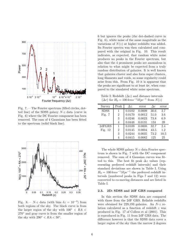
Fig. 7.— The Fourier spectrum (filled circles, dot-ted line) of the SDSS galaxy N -z data (curve inFig. 6) where the DC Fourier component has beenremoved. The sum of 4 Gaussians has been fittedto the spectrum (solid black line).

0

1000

2000

3000

0

200

400

0 0.05 0.1 0.15 0.2 0.25 0.3 0.35

N(z

): 1

00

o <

RA

< 2

70

o N(z

): 29

0o <

RA

< 5

0o

Redshift (z)

Fig. 8.— N -z data (with bins δz = 10−3) fromboth regions of the sky. The black curve is fromthe larger region of the sky with 100 < RA <270 and gray curve is from the smaller region ofthe sky with 290 < RA < 50.

6 but ignores the peaks (the dot-dashed curve inFig. 6), white noise of the same magnitude as thevariations of N(z) at higher redshifts was added.Its Fourier spectra was then calculated and com-pared with the original in Fig. 10. This resultindicates, as expected, that random white noiseproduces no peaks in the Fourier spectrum, butalso that the 4 prominent peaks are anomalous inrelation to what might be expected from a trulyrandom distribution of galaxies. It is well knownthat galaxies cluster and also form super clusters,long filaments and voids, so some regularity couldarise from this. From Fig. 10 it is apparent thatthe peaks are significant to at least 4σ, when com-pared to the simulated white noise spectrum.

Table I: Redshift (∆z) and distance intervals(∆r) for H0 = 100 kms−1Mpc−1 from N(z)

Survey Peak ∆z error ∆r error

SDSS 1 0.0102 0.0009 30.6 2.7Fig. 7 2 0.0170 0.0012 51.0 3.6

3 0.0246 0.0023 73.8 6.94 0.0448 0.0131 134 39

2dFGRS 1 0.0109 0.0008 32.7 2.4Fig. 12 2 0.0145 0.0004 43.5 1.2

3 0.0244 0.0035 73.2 10.54 0.0415 0.0082 125 25

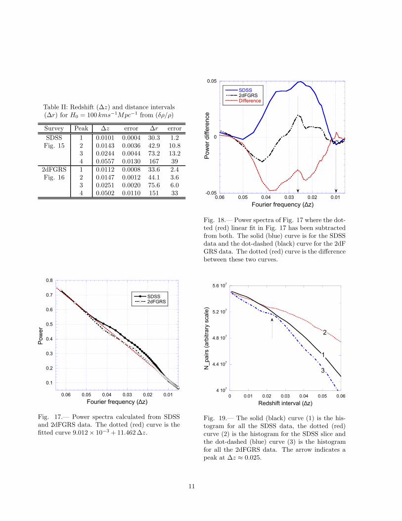
The whole SDSS galaxy N -z data Fourier spec-trum is shown in Fig. 7 with the DC componentremoved. The sum of 4 Gaussian curves was fit-ted to this. The best fit peak ∆z values (rep-resenting preferred redshift intervals) and theirstandard deviations are shown in Table I. UsingH0 = 100 kms−1Mpc−1 the preferred redshift in-tervals (numbered peaks in Figs 7 and 12) wereconverted to co-moving distances and are listed inTable I.

2.3. 2D: SDSS and 2dF GRS compared

In this section the SDSS data are comparedwith those from the 2dF GRS. Reliable redshiftswere obtained for 229,193 galaxies. An N -z re-lation calculated as a function of redshift z wasproduced in Fig. 17 of Colless et al (2001). Thisis reproduced in Fig. 11 from 2dF GRS data. Thedifference however is that the SDSS data cover alarger region of the sky than the narrow 2 degrees

6

0

200

400

600

800

2 10-3

4 10-3

6 10-3

10-2

3 10-2

5 10-2

Po

we

r

Fourier frequency (∆z)

1

2

3

Fig. 9.— Fourier transform of the N -z relationfrom Fig. 8. The solid (black) curve 1 is N -z forthe whole SDSS data set, the dashed (gray) curve2 is for the larger region of the sky with 100 <RA < 270 and the dotted (red) curve 3 is for thesmaller region of the sky with 290 < RA < 50,multiplied by a factor of 3.

10

100

1000

10-2

10-1

Po

we

r

Fourier frequency (∆z)

Fig. 10.— The black curve is the discrete Fourierspectrum of the SDSS galaxy N -z data (same asthe solid curve in Fig. 7) plotted as a functionFourier frequency converted to ∆z interval. Thegray curve is the Fourier spectrum of the whitenoise enhanced SDSS galaxyN -z data drawn fromthe polynomial fit in Fig. 6.

of the 2dF GRS data.

Nevertheless the Fourier spectrum of its N(z)data shows very similar peaks to that of the SDSSdata. See Fig. 12 where the peaks have been fit-ted with Gaussians, and Fig. 13 where the Fourierspectra from the SDSS and 2dF GRS data arecompared. The values for the numbered peaks,representing the preferred redshift intervals (∆z),are listed in Table I, along with their standard er-rors. Fig. 13 shows the Fourier spectra from thewhole SDSS data set (solid black curve), the whole2dF GRS data set (dotted curve) and a subset of49,044 SDSS data where the declination angle iswithin two degrees of the celestial equator (dashedcurve). The map of the data for the latter closelyresembles that of the 2dF GRS data as both aresampled close to the equatorial plane, and over thesame right ascension.

From Fig. 12 it is clear that peak number 2is not very significant in 2D samples. Its magni-tude is similar to the noise at the higher Fourierfrequencies. Notice though that the Fourier spec-trum of the 2dF GRS data (dotted curve) is similarto the narrow equatorial slice from the SDSS data(dashed curve). Also the real space map of 2dFGRS data seen in Fig. 18 of Colless et al (2001)is very similar to Figs 1 and 2. Both show similararcs and filament structures.

However peaks 1, 3 and 4 in Fig. 12 are all verysignificant. Also from a comparison of the data inTable I, it is clear that the values of the peaks1, 3 and 4 are consistent with the respective val-ues from the other data set, within their standarderrors.

Fig. 13 shows the Fourier spectra from thetwo surveys and except for peak number 2, theyoverlap. The height of peak number 3 from theSDSS was normalized to match peak number 3 ofthe 2dF GRS, so they could be compared. It isobserved that the Gaussian fits are a very goodmatch. Peak 3 is at a redshift interval ∆z =0.0246, which is most readily visible by eye in Fig.11. Peaks at number 4 have a large height differ-ence but similar line shapes.

Peak number 2 is strongly present in the Fourierspectrum from the whole SDSS data set but notsignificant in the 2dF GRS data. The Fourierspectrum of the thin equatorial slice from SDSS(dashed curve in Fig. 13) is similar to that of

7

0

500

1000

1500

2000

2500

0 0.05 0.1 0.15 0.2 0.25 0.3

N(z

)

Redshift (z)

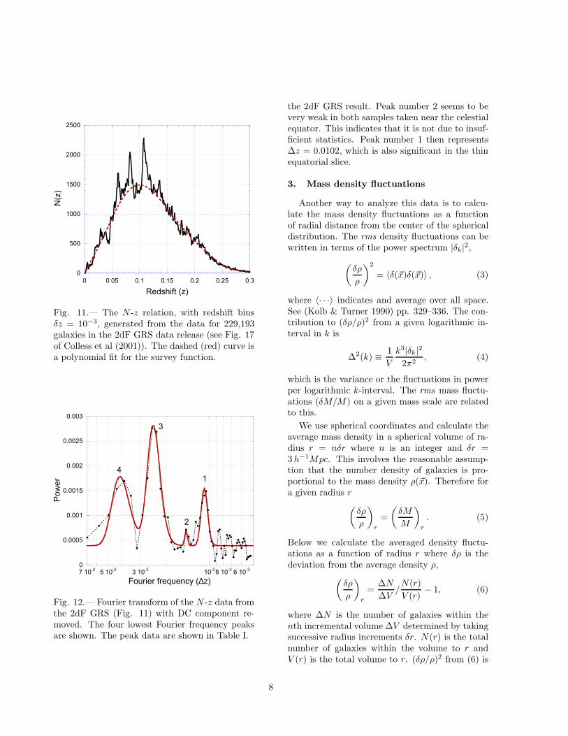
Fig. 11.— The N -z relation, with redshift binsδz = 10−3, generated from the data for 229,193galaxies in the 2dF GRS data release (see Fig. 17of Colless et al (2001)). The dashed (red) curve isa polynomial fit for the survey function.

0

0.0005

0.001

0.0015

0.002

0.0025

0.003

6 10-3

8 10-3

10-2

3 10-2

5 10-2

7 10-2

Po

we

r

Fourier frequency (∆z)

1

2

3

4

Fig. 12.— Fourier transform of the N -z data fromthe 2dF GRS (Fig. 11) with DC component re-moved. The four lowest Fourier frequency peaksare shown. The peak data are shown in Table I.

the 2dF GRS result. Peak number 2 seems to bevery weak in both samples taken near the celestialequator. This indicates that it is not due to insuf-ficient statistics. Peak number 1 then represents∆z = 0.0102, which is also significant in the thinequatorial slice.

3. Mass density fluctuations

Another way to analyze this data is to calcu-late the mass density fluctuations as a functionof radial distance from the center of the sphericaldistribution. The rms density fluctuations can bewritten in terms of the power spectrum |δk|2,

(

δρ

ρ

)2

= 〈δ(~x)δ(~x)〉 , (3)

where 〈· · ·〉 indicates and average over all space.See (Kolb & Turner 1990) pp. 329–336. The con-tribution to (δρ/ρ)2 from a given logarithmic in-terval in k is

∆2(k) ≡ 1

V

k3|δk|22π2

, (4)

which is the variance or the fluctuations in powerper logarithmic k-interval. The rms mass fluctu-ations (δM/M) on a given mass scale are relatedto this.

We use spherical coordinates and calculate theaverage mass density in a spherical volume of ra-dius r = nδr where n is an integer and δr =3 h−1Mpc. This involves the reasonable assump-tion that the number density of galaxies is pro-portional to the mass density ρ(~x). Therefore fora given radius r

(

δρ

ρ

)

r

=

(

δM

M

)

r

. (5)

Below we calculate the averaged density fluctu-ations as a function of radius r where δρ is thedeviation from the average density ρ,

(

δρ

ρ

)

r

=∆N

∆V/N(r)

V (r)− 1, (6)

where ∆N is the number of galaxies within thenth incremental volume ∆V determined by takingsuccessive radius increments δr. N(r) is the totalnumber of galaxies within the volume to r andV (r) is the total volume to r. (δρ/ρ)2 from (6) is

8

the variance ∆2(r) evaluated at r. From (6) weget

(

δρ

ρ

)

=∆N

∆Ωr2δr

∆Ωδr∑n

i=1(iδr)2

N(r)− 1, (7)

where the subscript has been dropped, ∆Ω =sinθ∆θ∆φ is the solid angle subtended by the nthvolume element, which is a constant for data sam-pled between fixed RA andDec angles. Therefore,

(

δρ

ρ

)

=∆N(n)

N(n)

∑ni=1 i

2

n2− 1, (8)

where r = nδr has been used, and N(n) is now afunction of the nth increment.

Since z = (H0/c)r it is equally valid to use red-shift intervals δz where z = nδz. For the radialincrement chosen here δr = 3 h−1Mpc the redshiftincrement δz = 10−3. It follows from (8) that

(

δρ

ρ

)

=∆N(n)

∑ni=1 ∆N(i)

(1 + n)(1 + 2n)

6n− 1, (9)

where ∆N(z) is now the number of galaxies in thenth redshift interval, where z = nδz.

The resulting density fluctuations (δρ/ρ) havebeen plotted in Fig. 14 as a function of redshift forboth the SDSS and 2dF GRS data. The square ofthese plots give you the variance ∆2(z) from whichthe power spectrum P (k) maybe derived with ap-plication of a windowing function and integratingover a logarithmic-k interval. Here we calculateP (z) in redshift units instead from

(

δM

M

)2

z0

=

∫

∞

0

∆2(z)W (z)2dz

z, (10)

with constants set to unity and where W (z) is thetop-hat windowing function,

W (z) =

1, z ≤ z00, z > z0.

(11)

The Fourier transforms of (δρ/ρ) and (δρ/ρ)2

were calculated using (1) with us = (δρ/ρ) and(δρ/ρ)2, respectively. Fig. 15 shows the resultsfor the SDSS data and Fig. 16 for the 2dF GRSdata. The labeled peaks are listed in Table II,where they have been calculated from Gaussianfits to the (δρ/ρ) curves. With the exception ofPeak 4, the rest are all in good agreement with

0

0.002

0.004

0.006

4 10-3

6 10-3

10-2

3 10-2

5 10-2

Po

we

r

Fourier frequency (∆z)

12

3

4

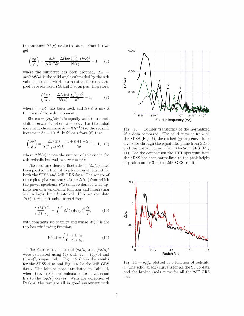
Fig. 13.— Fourier transforms of the normalizedN -z data compared. The solid curve is from allthe SDSS (Fig. 7), the dashed (green) curve froma 2 slice through the equatorial plane from SDSSand the dotted curve is from the 2dF GRS (Fig.11). For the comparison the FTT spectrum fromthe SDSS has been normalized to the peak heightof peak number 3 in the 2dF GRS result.

-1

-0.5

0

0.5

0 0.05 0.1 0.15 0.2

δρ/ρ

Redshift, z

Fig. 14.— δρ/ρ plotted as a function of redshift,z. The solid (black) curve is for all the SDSS dataand the broken (red) curve for all the 2dF GRSdata.

9

0

0.05

0.1

0.15

0.2

0.25

0

0.1

0.2

0.3

0.4

0.5

2 10-3

4 10-3

6 10-3

10-2

3 10-2

5 10-2

Po

we

r (δ

ρ/ρ)

Po

we

r (δρ/ρ)2

Fourier frequency (∆z)

1

3

4

2

Fig. 15.— The solid (black) curve is the squaredFourier transform of the SDSS (δρ/ρ) data fromFig. 14, plotted as a function of the redshift in-terval (∆z). The broken (red) curve is the Fouriertransform of (δρ/ρ)2 derived from the same SDSSdata. The most prominent peaks are labeled andcorrespond to the labels in Table I and II.

0

0.05

0.1

0.15

0.2

0.25

0

0.1

0.2

0.3

0.4

0.5

2 10-3

4 10-3

6 10-3

10-2

3 10-2

5 10-2

Po

we

r (δ

ρ/ρ)

Po

we

r (δρ/ρ)2

Fourier frequency (∆z)

1

2

3

4

Fig. 16.— The solid (black) curve is the squaredFourier transform of the 2dF GRS (δρ/ρ) datafrom Fig. 14, plotted as a function of the red-shift interval (∆z). The broken (red) curve isthe Fourier transform of (δρ/ρ)2 derived from thesame 2dF GRS data. The most prominent peaksare labeled and correspond to the labels in TableI and II.

peaks determined from FFT analysis of the N(z)counts in the previous section.

The power spectra P (z) from all the SDSS and2dF GRS redshift data are shown in Fig. 17. Bothcan be closely approximated by 11.462∆z. Bothpower spectra deviate from the linear dependenceand this can be seen in Fig. 18 where this lineardependence has been removed. The bottom (red)dotted curve is the difference between the two oth-ers. There is a large peak near ∆z0 = 0.026 and anindication of another near ∆z0 = 0.01, indicatedby the arrows.

4. Redshift separation between galaxies

Another way to determine if galaxies are sepa-rated by a periodic spatial interval is to build his-tograms by binning the number of pairs of galaxies(Npairs) that have the same separation in redshiftspace (∆z). Then look for over abundance peaksin the histograms. Since redshifts are measuredradially from the observer at the center of the dis-tribution this method detects spatial separationwith respect to that symmetry.

Three histograms were built and are shown inFig. 19:

1. all the 427,513 SDSS data from DR5 release,

2. the slice of 49,044 SDSS data taken fromwithin ±2 of the celestial equator, and,

3. all the 229,193 2dFGRS data taken within2 of the celestial equator with reliable red-shifts.

In Fig. 19 one can see slight ripples in thesecurves which represent above average correlations.Clearly this method is not very sensitive to dis-tinguish preferred separations against the back-ground of many pairs that have no such correla-tion. However one peak is clearly visible as indi-cated by the arrow; this is at ∆z ≈ 0.025.

By subtracting off a second order (quadratic)polynomial from these curves one can separate offthe background, enhance the weak features and seethe peaks more clearly, as shown in Figs 20 and21. Nevertheless they are still quite weak. In Fig.20 the solid (black) curve for Npairs from all theSDSS data shows peaks at ∆z = 0.0103 in goodagreement with the previous analyses, at ∆z =

10

Table II: Redshift (∆z) and distance intervals(∆r) for H0 = 100 kms−1Mpc−1 from (δρ/ρ)

Survey Peak ∆z error ∆r error

SDSS 1 0.0101 0.0004 30.3 1.2Fig. 15 2 0.0143 0.0036 42.9 10.8

3 0.0244 0.0044 73.2 13.24 0.0557 0.0130 167 39

2dFGRS 1 0.0112 0.0008 33.6 2.4Fig. 16 2 0.0147 0.0012 44.1 3.6

3 0.0251 0.0020 75.6 6.04 0.0502 0.0110 151 33

0.1

0.2

0.3

0.4

0.5

0.6

0.7

0.8

0.010.020.030.040.050.06

SDSS2dFGRS

Po

we

r

Fourier frequency (∆z)

Fig. 17.— Power spectra calculated from SDSSand 2dFGRS data. The dotted (red) curve is thefitted curve 9.012× 10−3 + 11.462∆z.

-0.05

0

0.05

0.010.020.030.040.050.06

SDSS2dFGRSDifference

Po

we

r d

iffe

ren

ce

Fourier frequency (∆z)

Fig. 18.— Power spectra of Fig. 17 where the dot-ted (red) linear fit in Fig. 17 has been subtractedfrom both. The solid (blue) curve is for the SDSSdata and the dot-dashed (black) curve for the 2dFGRS data. The dotted (red) curve is the differencebetween these two curves.

4 107

4.4 107

4.8 107

5.2 107

5.6 107

0 0.01 0.02 0.03 0.04 0.05 0.06

N_

pa

irs (

arb

itra

ry s

ca

le)

Redshift interval (∆z)

1

2

3

Fig. 19.— The solid (black) curve (1) is the his-togram for all the SDSS data, the dotted (red)curve (2) is the histogram for the SDSS slice andthe dot-dashed (blue) curve (3) is the histogramfor all the 2dFGRS data. The arrow indicates apeak at ∆z ≈ 0.025.

11

-4 105

-2 105

0

2 105

4 105

0 0.01 0.02 0.03 0.04 0.05 0.06 0.07

N_

pa

irs (

arb

itra

ry s

ca

le)

Redshift interval (∆z)

0.0

10

3

0.0

20

0

0.0

39

7

0.0

50

1

0.0

31

7

0.0

11

1

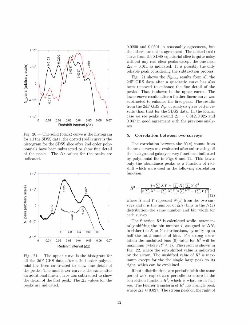
Fig. 20.— The solid (black) curve is the histogramfor all the SDSS data, the dotted (red) curve is thehistogram for the SDSS slice after 2nd order poly-nomials have been subtracted to show fine detailof the peaks. The ∆z values for the peaks areindicated.

-1 106

-5 105

0

5 105

1 106

0 0.01 0.02 0.03 0.04 0.05 0.06 0.07

N_

pa

irs (

arb

itra

ry s

ca

le)

Redshift interval (∆z)

0.0

25

0.0

47

0.0

12

0 0.01 0.02 0.03 0.04

0.0

12 0

.024

Fig. 21.— The upper curve is the histogram forall the 2dF GRS data after a 2nd order polyno-mial has been subtracted to show fine detail ofthe peaks. The inset lower curve is the same afteran additional linear curve was subtracted to showthe detail of the first peak. The ∆z values for thepeaks are indicated.

0.0200 and 0.0501 in reasonably agreement, butthe others are not in agreement. The dotted (red)curve from the SDSS equatorial slice is quite noisywithout any real clear peaks except the one near∆z = 0.011 as indicated. It is possibly the onlyreliable peak considering the subtraction process.

Fig. 21 shows the Npairs results from all the2dF GRS data after a quadratic curve has alsobeen removed to enhance the fine detail of thepeaks. That is shown in the upper curve. Thelower curve results after a further linear curve wassubtracted to enhance the first peak. The resultsfrom the 2dF GRS Npairs analysis gives better re-sults than that for the SDSS data. In the formercase we see peaks around ∆z = 0.012, 0.025 and0.047 in good agreement with the previous analy-ses.

5. Correlation between two surveys

The correlation between the N(z) counts fromthe two surveys was evaluated after subtracting offthe background galaxy survey functions, indicatedby polynomial fits in Figs 6 and 11. This leavesonly the abundance peaks as a function of red-shift which were used in the following correlationfunction.

R2 =(n

∑

XY − (∑

X)(∑

Y ))2

[n∑

X2 − (∑

X)2][n∑

Y 2 − (∑

Y )2],

(12)where X and Y represent N(z) from the two sur-veys and n is the number of ∆Ni bins in the N(z)distribution–the same number and bin width foreach survey.

The function R2 is calculated while incremen-tally shifting the bin number i, assigned to ∆Ni

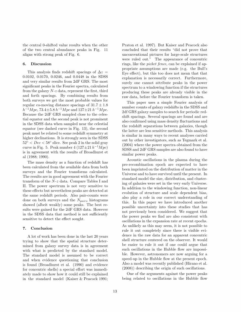
in either the X or Y distributions, by unity up tohalf the total number of bins. For strong corre-lation the unshifted bins (0) value for R2 will bemaximum (where R2 ≤ 1). The result is shown inFig. 22, where the zero shifted value is indicatedby the arrow. The unshifted value of R2 is max-imum except for the the single large peak to itsright, which can be explained.

If both distributions are periodic with the sameperiod we’d expect also periodic structure in thecorrelation function R2, which is what we in factsee. The Fourier transform of R2 has a single peakwhere ∆z ≈ 0.027. The strong peak on the right of

12

the central 0-shifted value results when the otherof the two central abundance peaks in Fig. 11aligns with strong peak of Fig. 6.

6. Discussion

This analysis finds redshift spacings of ∆z =0.0102, 0.0170, 0.0246, and 0.0448 in the SDSSand very similar results from 2dF GRS. The mostsignificant peaks in the Fourier spectra, calculatedfrom the galaxyN -z data, represent the first, thirdand forth spacings. By combining results fromboth surveys we get the most probable values forregular co-moving distance spacings of 31.7 ± 1.8h−1Mpc, 73.4±5.8 h−1Mpc and 127±21 h−1Mpc.Because the 2dF GRS sampled close to the celes-tial equator and the second peak is not prominentin the SDSS data when sampled near the celestialequator (see dashed curve in Fig. 13), the secondpeak must be related to some redshift symmetry athigher declinations. It is strongly seen in the SDSS52 < Dec < 58 slice. See peak 2 in the solid graycurve in Fig. 5. Peak number 4 (127±21 h−1Mpc)is in agreement with the results of Broadhurst etal (1988; 1990).

The mass density as a function of redshift hasbeen calculated from the available data from bothsurveys and the Fourier transforms calculated.The results are in good agreement with the Fouriertransform of the N -z data. Compare Tables I andII. The power spectrum is not very sensitive tothese effects but nevertheless peaks are detected atthe same redshift periods. Also pair-counts weredone on both surveys and the Npairs histogramsshowed (albeit weakly) some peaks. The best re-sults were gained for the 2dF GRS data. Howeverin the SDSS data that method is not sufficientlysensitive to detect the effect sought.

7. Conclusion

A lot of work has been done in the last 20 yearstrying to show that the spatial structure deter-mined from galaxy survey data is in agreementwith what is predicted by the standard model.The standard model is assumed to be correctand when evidence questioning that conclusionis found (Broadhurst et al. (1990) and evidencefor concentric shells) a special effort was immedi-ately made to show how it could still be explainedin the standard model (Kaiser & Peacock 1991;

Praton et al. 1997). But Kaiser and Peacock alsoconcluded that their results “did not prove thatunconventional pictures for large-scale structureswere ruled out.” The appearance of concentricrings, like the picket fence, can be explained if ap-propriate assumptions are made (e.g. the Bull’sEye effect), but this too does not mean that thatexplanation is necessarily correct. Furthermore,surely one cannot attribute peaks in the powerspectrum to a windowing function if the structuresproducing these peaks are already visible in theraw data, before the Fourier transform is taken.

This paper uses a simple Fourier analysis ofnumber counts of galaxy redshifts in the SDSS and2df GRS galaxy samples to search for periodic red-shift spacings. Several spacings are found and arealso confirmed using mass density fluctuations andthe redshift separations between galaxies, thoughthe latter are less sensitive methods. This analysisis similar in many ways to recent analyses carriedout by other investigators, such as Tegmark et al.(2004) where the power spectra obtained from theSDSS and 2dF GRS samples are also found to havesimilar power peaks.

Acoustic oscillations in the plasma during thepre-recombination epoch are expected to havebeen imprinted on the distribution of matter in theUniverse and to have survived until the present. Instandard model the size, distribution, and cluster-ing of galaxies were set in the very early Universe.In addition to the windowing function, non-linearevolution of structure and scale dependent bias,also play a role in our correct understanding ofthis. In this paper we have introduced anotherpossible uncertainty into these studies that hasnot previously been considered. We suggest thatthe power peaks we find are also consistent withoscillations in the expansion rate at recent epochs.As unlikely as this may seem, it is not possible torule it out completely since there is visible evi-dence in the raw data for an apparent concentricshell structure centered on the observer. It wouldbe easier to rule it out if one could argue thatsuch oscillations in the Hubble flow are impossi-ble. However, astronomers are now arguing for aspeed-up in the Hubble flow at the present epoch.Also a model was recently published (Hirano et al.(2008)) describing the origin of such oscillations.

One of the arguments against the power peaksbeing related to oscillations in the Hubble flow

13

is the fact that the P (k) distribution is a rea-sonable fit to what is predicted for the standardmodel. However, this does not rule oscillationsout also. If there were no density fluctuations(no clustering etc.), and the Universe was madeup of a completely uniform distribution of galax-ies, oscillations in the raw Hubble flow data wouldlikely result in the appearance of concentric shellsof apparent low and high density surrounding theobserver because of the light travel time. To de-tect this there may be no need to use a windowingfunction. However, even if oscillations are presentin the low-redshift Universe, any accurate modelwould also have to account for the density fluctu-ations (due to clusters, super clusters, etc.) thatare also clearly visible.

And some have argued that the peaks foundin this paper are just the scale sizes of clus-tering (Kaiser & Peacock 1991; Mo et al. 1992;Gonzalez et al. 2000); this was considered im-probable by (Yoshida et al 2001) but a similaranalysis needs to be performed on a larger dataset in order to test this. Nevertheless the meth-ods applied to the data here are consistent withthe Universe undergoing oscillations in its expan-sion rate over past epochs. This means in redshiftspace there are preferred redshifts where galaxiesare more dense due to a slower expansion rate atthose epochs.

8. Acknowledgments

We would like to thank F. Oliveira and T.Potter for valuable discussions and assisting JGHin obtaining SDSS/2dF GRS data, as well asP. Abbott for help with Mathematica software.The concluding remarks were largely written fromcomments made by one anonymous reviewer, forwhich we are very thankful. This work has beensupported by the Australian Research Council.

Funding for the SDSS and SDSS-II has beenprovided by the Alfred P. Sloan Foundation, theParticipating Institutions, the National ScienceFoundation, the U.S. Department of Energy, theNational Aeronautics and Space Administration,the Japanese Monbukagakusho, the Max PlanckSociety, and the Higher Education Funding Coun-cil for England.

The SDSS is managed by the AstrophysicalResearch Consortium for the Participating Insti-

tutions. The Participating Institutions are theAmerican Museum of Natural History, Astro-physical Institute Potsdam, University of Basel,University of Cambridge, Case Western ReserveUniversity, University of Chicago, Drexel Univer-sity, Fermilab, the Institute for Advanced Study,the Japan Participation Group, Johns HopkinsUniversity, the Joint Institute for Nuclear As-trophysics, the Kavli Institute for Particle As-trophysics and Cosmology, the Korean Scien-tist Group, the Chinese Academy of Sciences(LAMOST), Los Alamos National Laboratory,the Max-Planck-Institute for Astronomy (MPIA),the Max-Planck-Institute for Astrophysics (MPA),New Mexico State University, Ohio State Uni-versity, University of Pittsburgh, University ofPortsmouth, Princeton University, the UnitedStates Naval Observatory, and the University ofWashington.

REFERENCES

2 degree Field Galaxy Redshift Survey (2dF GRS),a joint UK-Australian project. The 2dF GRSwebsite is www.aao.gov.au/2df/.

C. Baugh, “Correlation function and power spec-tra in cosmology,” in Encycl. of Astronomy and

Astrophysics (IOP Publishing, Bristol, 2006)

T.J. Broadhurst, R.S. Ellis, T. Shanks, MNRAS

235, 827, 1988

T.J. Broadhurst, R.S. Ellis, D.C. Koo, and A.S.Szalay, Nature 343, 726, 1990

M.M. Colless et al. Mon. Not. R. Astron. Soc. 328,1039, 2001

J.A. Gonzalez, H. Quevedo, M. Salgado, and D.Sudarsky, Astron. Astrophys. 362, 835, 2000

A.J.S. Hamilton, M. Tegmark, N. Padmanabhan,Mon. Not. R. Astron. Soc. 317, L23, 2000

K. Hirano, K. Kawabata and Z. Komiya, Ap&SS,315, 53, 2008

N. Kaiser and J.A. Peacock, Ap. J. 379, 482, 1991

E.W. Kolb, M.S. Turner,The Early Universe,(Addison-Wesley Publishing, Redwood City,Calif., 1990)

14

A.L. Melott, P. Coles, H.A. Feldman, and B. Wil-hite, Ap. J. 496, L85, 1998

H.J. Mo, Z.G. Deng, X.Y. Xia, P. Schiller, G.Borner, Astron. Astrophys. 257, 1, 1992

P.J.E. Peebles, in The Large Scale Structure of

the Universe (Princeton, Princeton UniversityPress, 1980), p.174

E.A. Praton, A.L. Melott, and M.Q. McKee, Ap.J. 479, L15, 1997

Astrophysical Research Consortium (ARC) andthe Sloan Digital Sky Survey (SDSS) Collab-oration. The SDSS Web site is www.sdss.org.

M. Tegmark et al., Ap. J. 606, 702, 2004

B.C. Thomas, A.L. Melott, H.A. Feldman, andS.F. Shandarin, Ap. J. 601, 28, 2004

N. Yoshida et al. Mon. Not. R. Astron. Soc. 325,803, 2001

This 2-column preprint was prepared with the AAS LATEX

macros v5.2.

0

0.05

0.1

0.15

0.2

0.25

0.3

-200 -150 -100 -50 0 50 100 150 200

Co

rre

latio

n, R

2

Shift (bins)

Fig. 22.— The correlation function R2 betweenthe abundance distributions of SDSS and 2dFGRS. The zero shifted correlation coefficient isshown by the arrow.

15