Science for Clean Energy

Grant agreement No. 764810

Science for Clean Energy

H2020-LCE-2017-RES-CCS-RIA

Competitive low-carbon energy

D3.3

A ready to operate Laser Isotope Ratiometer configured for the field tests

WP 3 – Instruments and Tools: Development and Deployment

Due date of deliverable Month 24 - September 2019

Actual submission date 02 / 09/ 2019

Start date of project 1st September 2017

Duration 36 months

Lead beneficiary MIRICO

Deliverable D3.3

CO Page 2 of 42 Version 1.3

Last editor Natalie Nestorowicz

Contributors Nicholas Paul (NP), Richard Brownsword (RB), Richard Kovacich (RK), Damien Wiedmann (DW), Arun Kannath (AK), Mohammed Belal (MB), Johnny Chu (JC), Annika Voss (AV)

Dissemination level Confidential (CO)

This Project has received funding from the European Union’s Horizon 2020 research and innovation programme under grant agreement no. 764810

Deliverable D3.3


History of the changes

Version Date Released by Comments

1.0 30-08-2019 NP First draft completed

1.1 30-08-2019 RK Edited

1.2 01-09-2019 DW, RK Edited

1.3 05-09-2019 DW Edited by AS and Damien Weidmann DW

Deliverable D3.3


Table of contents

1 Introduction .......................................................................................................... 7

1.1 General context .......................................................................................... 7

1.2 Deliverable objectives ................................................................................. 8

2 Methodological approach ..................................................................................... 9

2.1 Isotopic line selection ................................................................................. 9

2.1.1 Optimum pressure and temperature operation ............................................... 10

2.2 Survey of CarbFix 1 field trial site ............................................................. 12

2.3 Main unit assemblies ................................................................................ 13

2.3.1 Optical base assembly ........................................................................................ 13

2.3.2 Acquisition board, power supply plate and casing ............................................ 16

2.4 Gas cell designs ......................................................................................... 17

2.4.1 Static gas cell assembly ...................................................................................... 17

2.4.2 Multipass cell assembly and modelling ............................................................. 17

2.4.3 Hermetic fixing of optical elements ................................................................... 20

2.4.4 Extractive gas cell design ................................................................................... 21

2.5 Modified optics for closed path detection and software ......................... 21

2.5.1 Sample-detector subassembly ........................................................................... 21

2.5.2 Software for data acquisition ............................................................................ 21

2.6 Signal processing approach ...................................................................... 22

3 Summary of activities and research findings ...................................................... 23

3.1 Integration to a single portable unit ......................................................... 23

3.2 LDS performance for isotopic analysis ...................................................... 25

3.3 Sample cell design: static and multipass .................................................. 30

3.3.1 3.3.0 Manufacture of multifaceted multipass cells ........................................... 30

3.3.2 Modelling of beam propagation in the short OPL multipass cell ...................... 32

3.3.3 Multipass cell hermeticity .................................................................................. 33

3.3.4 Preparation of static pure CO2 samples: sealed static cells ............................... 34

3.4 Phase spectra acquisition and fitting ........................................................ 36

3.4.1 Spectrum acquisition ......................................................................................... 36

3.4.2 Phase forward model ......................................................................................... 38

Deliverable D3.3


4 Conclusions and future steps .............................................................................. 41

5 Bibliographical references................................................................................... 42

Deliverable D3.3


Key word list

Gas sensing, isotope ratio, CO2 detection, carbon fixation, infrared, dispersion spectroscopy, lasers, optical dispersion, intraband cascade lasers, phase modelling, portable instrument, carbon fixation, extractive gas system, gas cell.

Definitions and acronyms Acronyms Definitions

AM

AOM

CAD

CNRS

FM

GUI

ICL

LDS

NIS

OAP

ORION

QCL

RF

S4CE

MFM

ROC

SNR

TEC

Amplitude modulation

Acousto-optic modulator

Computer assisted design

Centre national de la recherche scientifique

Frequency modulation

Graphical user interface

Interband cascade laser

Laser Dispersion Spectroscopy

Naftna industrija Srbije

Off-axis parabolic mirror

Trademark name for planned

LDS-100 commercialisation

Quantum cascade laser

Radio frequency

Science 4 Clean Energy

Multi-faceted mirror

Radius of curvature

Signal to noise ratio

Thermoelectric cooler

WP Work Package

OPL Optical path length

Deliverable D3.3


1 Introduction

Deliverable D3.3 is the production/demonstration of a portable, laser dispersion spectrometer prototype tailored to the isotopic ratio analysis of CO2. The prototype presented herein is a milestone towards the more detailed/sophisticated deliverable due in March 2020, which involves a field trial at the Reykjavik Energy CarbFix 1 test site. The prototype is associated with the previously reported work package WP 3 task 3.2 (ex 3.4). It is also closely linked to the material in WP 6, Task 6.4 that involves the methods for gas sensor calibration and laboratory validation.

1.1 General context

One of the objectives of the Science for Clean Energy (S4CE) project is to quantify eventual CO2 emissions in varied situations. One proposed scenario was CO2 leakage from industrial piping and operations, where the concentration levels are barely above ambient. Another avenue is the quantification of CO2 to be injected into underground fixation processes (e.g., carbon sequestration or CO2-based enhanced hydrocarbon recovery operations). The CarbFix-1 process is a technique of CO2 fixation using reactive basalt, developed by teams based at Reykjavik Energy, University of Iceland, Centre national de la recherche scientifique (CNRS) Tolouse, and the Earth Institute at Columbia University.[1] This process has the potential to become a viable avenue of controlling industrial levels of CO2 production. Its basis lies on the thermodynamically favourable pathway of CO2 fixation using basalt rocks to form thermodynamically inert carbonate minerals and store them underground.[2] Although, as any other process that seeks CO2 fixation and underground storage, the CarbFix-1 project faces possible risks such as CO2 leakage, induced seismic activity and underground water contamination, it nevertheless demonstrates an industrially scalable, low intensity condition approach for isolating CO2 into a transportable, easy to handle material. Furthermore, the project potentially could mitigate costs associated with the reduction in gaseous emissions as produced CO2 gas emissions (containing other gases and contaminants) are potentially captured and converted directly to a solid form.

Previous methods of detection and monitoring CO2 uptake in the CarbFix process depended on the use of isotopically labelled carbon (C13 and C14) in tandem with sampled gas chromatograph and high resolution mass spectrometry analysis,[3] or indirect methods that employ sulphate injection to aqueous CO2 or measure alkali earth cation fractions.[3-5]

S4CE aims to develop a high resolution, high sensitivity instrument capable of quantification of gas isotope ratios for direct observation of gas release and uptake. The gas sample extractive instrument, which is based on the method of laser dispersion spectroscopy (LDS), will be used to monitor in real time the progress of the CO2 content in the CarbFix1 injection fluid using the planned sampling system shown in Figure 1. The original fluid will be mostly dissolved, aqueous CO2 (99.5%) with trace H2S (0.5%) that will be scrubbed by a charcoal filter. The instrument will be designed for to accommodate continuous, extractive sampling and measurement of the aqueous CO2, have sufficient sampling rate (ms to few s range) and robust to fluctuating ambient temperature and mild chemical corrosion over an extended period of experimental time (15-90 days).

The final instrument will comply with all the requirements listed. For the purpose of the current deliverable, the scope is to develop a working, transportable unit that demonstrates

Deliverable D3.3


the first set of capabilities and/or requirements necessary towards moving the lab benchtop, academic system to a fully functional, industrial unit that can operate in the field.

Figure 1: Schematic of the planned field trial experiment at Reykjavik Energy site. Shaded red regions highlight aspects that MIRICO will be responsible for. MIRICO has been charged with designing the programs to operate the remote control shutoff valve. The other highlighted region represents the instrument. Design of the extractive system (cell and flow-pressure control) and the closed path laser dispersion spectrometer.

1.2 Deliverable objectives

The objective of Deliverable 3.3 is to provide the basis for constructing the first transportable prototype of the isotope ratiometer. In addition, there are requirements involving the validation of data analytic and software methods that will be used for the full instrument, which are crucial to the post-processing required to enable high accuracy quantification of the isotope ratios. The latter aspect links to deliverables part of WP 6.

Deliverable D3.3


2 Methodological approach

Construction of the prototype Laser Isotope Ratiometer is based upon expansion of the new LDS-100 units that have been designed and tested for the open path, laser dispersion spectrometer (to be named ORION for the planned commercialisation, and referred to as herein) including optical apparatus, electronic acquisition and power supply units. The LDS-100 units are described in some details in Deliverable 3.4. Adaptation of the design to the present requirements involves removal of the scanning turret head for open path measurement and incorporation of the detection module into the same unit as the optical apparatus. Instrument modifications include the extractive gas cell measurement apparatus and a sealed, solid to solid contact thermal control system. The prototype will only utilize simple test ideas for the sample apparatus and thermal control, namely use of static gas samples (non-flow, non-extractive) at the required CO2 concentrations and simple metal to metal contact cooling, specifically mounting the unit modules (optical, acquisition and power supply) in direct contact with a metallic casing.

Key steps to the prototype development are summarised as follows:

- Isotopic lines selection - Determine the instrument requirements for the planned field trial - Main unit assemblies - Static gas cell assembly - Multipass cell development including modelling, manufacturing and testing - Extractive gas cell development - Sample-detector subassembly - Software for data acquisition - Signal processing approach

2.1 Isotopic line selection

A key part of the instrument design is underpinned by the optimum choice of the isotopologue transitions to be used for the spectroscopic measurement. The corresponding line selection was done using the methodology described by Weidmann et al., [9] which investigated the spectral region between 2240 and 2310 cm-1. The main result of the method, broadly speaking, is to find adjacent 13CO2 and 12CO2 lines that have similar line intensities of adequate strength and wavenumber separation. This line filtering analysis gives back 6 potential line pairs spread over 2291 to 2304 cm-1. A transmission spectrum showing these 6 line pairs is shown in Figure 2 showing that the optimum line pair is located at ~2296 cm-1. The pair at 2298 cm-1 is disregarded due to overlap and the pair at 2302.5 cm-

1 is disregarded due to intensity difference. Note that the line intensities are around 2 to 4 10-20.

Deliverable D3.3


Figure 2: Calculated transmission spectrum for 1% CO2, 10 cm path length, 100 Torr pressure.

There are potential absorbing interferences in this region, which include: N2O (3.4 10-22 cm-

1/mole/cm-2), NH3 (1.9 10-22), HI (5.2 10-22), CH3Cl (1.4 10-23), PH3 (9.2 10-20), H2S (1.3 10-22).

However, it is not anticipated, for the application at hand, that these interfering gases will be present at any significant level in the gas samples at the field test sites.

2.1.1 Optimum pressure and temperature operation

Using the line pair selected (see Figure 2), a systematic analysis of pressure and temperature parameters was conducted using an ideal instrument simulator. The objective of this activity consists of determining for a selection of relevant concentrations, the expected ideal

precision on the 13C for a range of pressures and path lengths.

The methodology is described in the flow chart of Figure 3.

Figure 3: Flowchart of the top-level algorithm used to estimate the instrument precision.

Example output data are shown in Figure 4 for four CO2 concentrations spanning from 100

ppmv to 10 %. These plots show the expected ideal 13C precision as function of pressure and path length. It is noted that the optimized pressure to conduct a measurement varies with CO2 concentration: 70 Torr for 100 ppmv, 90 Torr for 0.1%, 30 Torr for 1%, and 20 Torr for 10%.

Based on these results, and assuming a variable pressure will be encountered in practical applications, it seems that a fixed path length system could be appropriate for developing the prototype. For example, a 20 cm path length system would give the following precisions: 6.5‰, 1.0‰, 0.2‰, 0.1‰ at respectively 100ppmv, 0.1%, 1% and 10% CO2 concentration.

Deliverable D3.3


This precision implies that a 0.25‰ precision requirement can be fulfilled for the following measurement times: 25s, 0.6s, 0.023s, and 0.006s.

Figure 4: Example plots of 13C precision as function of pressure and path length for four CO2 sample concentrations.

We conclude from this analysis that the laser isotope ratiometer should include means of adjusting the sample pressure from 20 to 90 Torr to optimise the measurement performance for the expected CO2 concentration, implying that a fixed path cell is useable. This function may be provided by a digital pressure controller, as shown in Figure 1.

For the CarbFix 1 field trial, a CO2 gas concentration of ~99.5% is expected and the trend of this analysis with respect to gas concentration indicates that a very rapid and high precision measurement can be achieved with a short cell of ~1cm, which will also be required to avoid excessive optical opacity from the CO2 line absorption. Additional simulations will be required to inform the optimum instrument configuration in this situation.

Deliverable D3.3


2.2 Survey of CarbFix 1 field trial site

A site visit was conducted in June 2019 to the Reykjavik Energy CarbFix 1 test site, which is at the Hellisheidi geo-thermal power plant in Iceland. This visit had the scope of surveying the planned field trials of the laser isotope ratiometer and the open path instrument described in Deliverable 6.1. The site survey findings are summarised below:

• Measurement sites at HE-31 monitoring well and CarbFix 1 injection well

• High level of acoustic noise within both igloos (see Figure 5).

• Piping keeps temperature above ambient - never below 15oC and can exceed 30oC

• Residual atmospheric H2S promoting increased corrosion over time - more abundant at injection well

• Considered available infrastructure for deployment – power, data link etc.

• Captured H&S training requirements for MIRICO staff to carry out deployment in WP7

• Sample expected to be 99.5% CO2 and 0.5% H2S (scrubbed) – to be confirmed following installation of sampling system by OR

• Long trend, 15 days to 3 months measurements needed – to allow for fluid transport from injection well to monitoring well

• Condensation risk – heated setup within MIRICO instrument. Though may be avoided using instrument purge with dry gas e.g. compressed air line.

• MIRICO responsible for remote control of operable shut off valve

Figure 5: Photographs of CarbFix 1 field trial site

Deliverable D3.3


2.3 Main unit assemblies

Much of the laser isotope ratiometer design is based on the ORION system, which was designed to be robust against environmental conditions. The optical base, acquisition plate and power supply plate are nigh on identical to the ORION system with only a few modifications. In brief, the system has utilised the same optical base with one modification: substitution of the expanding off-axis parabolic (OAP) pair and the exit control mirrors for a simple sample-detector subunit assembly. The same acquisition and power supply boards have also been used. As the system is not an open path system, the beam distance to detector is much, much shorter and simpler. The idea is that the sample-detector sub assembly will be the only part of the optical base that will require changing. For the end of August 2019, a sub assembly which enables static gas cell measurements has been built. For the longer-term target in March 2020, during which the field trial in collaboration with Reykjavik Energy is planned, we will modify this sub-assembly (or create a new one) to house a well-sealed, extractive gas sample system.

2.3.1 Optical base assembly

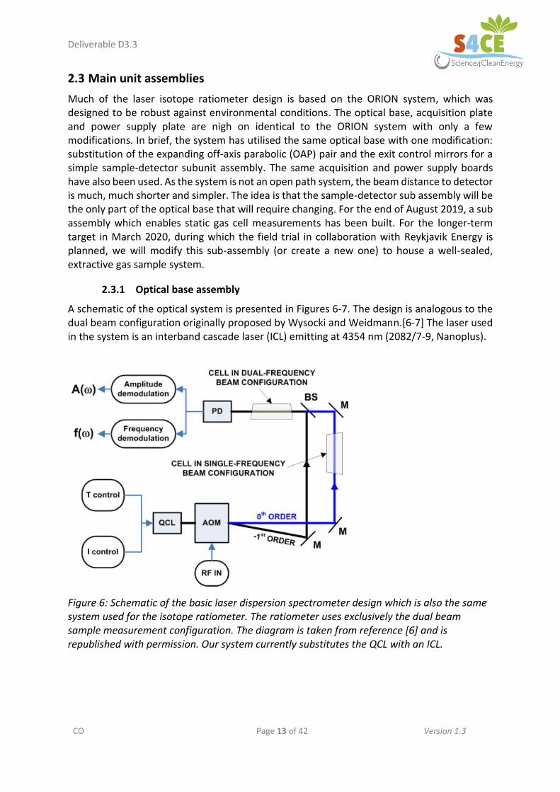
A schematic of the optical system is presented in Figures 6-7. The design is analogous to the dual beam configuration originally proposed by Wysocki and Weidmann.[6-7] The laser used in the system is an interband cascade laser (ICL) emitting at 4354 nm (2082/7-9, Nanoplus).

Figure 6: Schematic of the basic laser dispersion spectrometer design which is also the same system used for the isotope ratiometer. The ratiometer uses exclusively the dual beam sample measurement configuration. The diagram is taken from reference [6] and is republished with permission. Our system currently substitutes the QCL with an ICL.

Deliverable D3.3


Figure 7: eDrawings representation of the isotope ratiometer designed. The optical system design contains the same optical base (light purple) along with identical laser housing (peach), beam collimation OAP pair (pink), AOM and beam delay (olive) subassemblies. The visual substitutes in a basic sample-detector subassembly (grey). Minor errors or misrepresentations include the presence of the 2-inch gold mirror and mount used for directing the beam out of the original ORION system and the mechanical mirror (silver item between AOM-beam delay and sample-detector subassemblies). Both parts are irrelevant for the isotope ratiometer system, but neither intrudes on the necessary area for modification.

Among other considerations described above, the wavelength has been chosen so that there is a reasonable overlap with C12 and C13 peaks at 2296.55 cm-1 and 2295.84 cm-1, respectively. The output is captured and slowly focused by a planoconvex lens and the measured output of the laser is ~3.1 mW at 44 mA and 10 °C (datasheet specified typical operating parameters). The small (~10%) drop in power from the quoted value of 3.4 mW likely arises from imperfect transmission via the laser head focusing lens. The beam output was adjusted to give a homogeneous profile and a current, wavelength, temperature profile was taken (Figures 8 and 9). Beam characterisation of the laser head, in the machined laser house, was taken before installation with the main sub assembly. Note that in Figure 6 there is an open space on the laser head subassembly for a second laser. Typical open path ORION systems come equipped for two gas measurements (currently CH4 and CO2), and it is conceivable that in the future the isotope system will be upgraded to a two laser platform. However, for the purposes of the application envisioned in the present Deliverable, the system was configured to house just one laser.

Deliverable D3.3


Figure 8: Wavelength vs current plot of the ICL 2082/7-9 laser used in the isotope ratiometer. Data was taken within the specified 5-15 °C operating range.

Figure 9: Power vs current plot of the ICL 2082/7-9 laser used in the isotope ratiometer. Data was taken within the specified 5-15 °C operating range.

Deliverable D3.3


After the focusing lens, the beam is sent through an OAP pair to induce a focus into the acousto-optic modulator (AOM) crystal (Figure 7). The AOM is a Ge crystal unit used to both generate the dual beam configuration and to frequency shift the first order with respect to the zeroth order beam. The radio frequency (RF) signal used was set to 166.7 MHz. Collection and recombination of the two frequency shifted beams after the AOM, for a collinear-coplanar overlapped beam occurs via use of a wedged beamsplitter. The zeroth order beam passes via a translation stage mounted corner cube mirror prior to beam recombination. The stage is used to set the path lengths of each interferometer arm to be equivalent and thus minimise background offset in the frequency modulation (FM) trace.

Collinearity and coplanarity of the two beams are diagnosed using a pyroelectric beam imaging camera (Pyrocam IIIHR, Ophir). Once the two-beam overlap alignment is complete, the combined beams are sent into the sample-detector subassembly and finally focused onto the detector (PVI-4TE-5-0.5x0.5, Vigo) using an OAP.

2.3.2 Acquisition board, power supply plate and casing

The acquisition board consists of an Alpha250 control board (Koheron) connected to a homebuilt circuit board that acts as an extension/relay unit for multiple subsystems including laser driver boards (DRV200S-A-200 and QCL100, Koheron), thermoelectric cooling (TEC. HTC1500, Wavelength Electronics) drivers and bandpass filters (ZABP-184-S+ and ZX75LP-216-S+, Mini-Circuits). The Alpha250 was connected to a work laptop via router as to assign dynamic IP and the base program is written in Python (Anaconda Distribution, Windows version, Python 3.7). The web interface package, Bokeh, was used to write the graphical user interface (GUI) that permits user control of the instrument for experimental parameters, data visualisation and saving raw data. The lasers can be run up to 200 mA (DRV200S-A-200) or 650 mA (QCL100-A-500) of drive current. For this report, the DRV200 module was used as the current limits of the laser were well below 200 mA. The power supply plate houses several voltage supplies (12, 24 and 48 V) to power the various components. The network router and junction units are also housed on the plate. For the Orion open path systems, the power supply plate powers the optical layer, detection layer and the turret head; however for the isotope system the optical and detector layer are merged onto one assembly and no turret head is needed, so the voltage supply only powers the optical assembly primarily. This consists of laser, AOM, detector, RF signal generator and amplifier. Calculations of the Orion open path system shows approximately 200 W of thermal energy generated by the system, most of it arising from the electronics. Without the turret head and the voltage supply module to drive it, it is estimated that the thermal energy generated will be reduced to about 130-140 W. The casing used to house the instrument is an in-house modified IP66 grade wall cabinet (ES46664516/G, Canford). The cabinet is made of 1.5 mm folded steel. The case is machined to mount the acquisition and power supply plates to the interior. The optical base is mounted via 4 threads to a 2 mm thick support plate. To assist in weight distribution, the plate has been modified with a series of spacers that secure the support plate to the back of the cabinet. In addition, the optical base is vibrationally isolated using anti-vibration cylinders. Heat dissipation from the acquisition board occurs into the steel case as the board is mounted in direct contact to the case.

Deliverable D3.3


2.4 Gas cell designs

2.4.1 Static gas cell assembly

As the field demonstration will be carried out on near-pure CO2, a mitigation for the lack of a hermetic flow cell would be to use existing 1-cm sealed glass cells with a static CO2 sample. Three cells, numbered 2, 4 and 5 were available and were leak-tested against the base leak rate of a vacuum system. The cells were connected to the vacuum line using a Legris 4-mm push-fit connector as illustrated in Figure 10.

Figure 10: static gas cell connected to the gas/vacuum line for filling and leakage tests (left). The gas cell is sealed by blow torch melting the glass tube inlet creating a permanent seal (right).

2.4.2 Multipass cell assembly and modelling

The multipass cell flow cell was conceived to assist in the initial aims for the S4CE project

when Naftna industrija Srbije (NIS) was a partner with a goal to measure CO2 fluctuations above ambient (0.1-1‰ fluctuations), which requires a much longer optical path to achieve the sensitivity. Therefore, a novel multipass cell was designed and manufactured using diamond turned multifaceted mirrors, for which a patent has been filed.

Modelling of a high beam density variant of the multifaceted mirror (MFM) multipass cell was done to find the optimum parameters, such as mirror focal length and positions, and to understand the alignment tolerances required. The modelling was done using our own code in Python and also with Zemax ray tracing software. An example result that fixes the focus position in the centre of the cell and the mirror ROC equal to the mirror separation is shown in Figure 11 using the following input parameters:

Cell length 179.0 mm

Facet diameter 5.0 mm

Gap 0.25 mm

Number of facets 6

Facet tilt angle (derived) 0.84 degrees

ROC 179.0 mm

f (derived) 89.5 mm

focus position 0.5 (centre of cell)

Deliverable D3.3


Note that the number of passes of the MFM multipass cell can be summarised by the following formula, where M and N are the number of facets in the vertical and horizontal directions:

𝑁𝑢𝑚𝑏𝑒𝑟 𝑜𝑓 𝑝𝑎𝑠𝑠𝑒𝑠 = 2(𝑀 × 𝑁) − 1

The optical path length is then the number of passes multiplied by the cell length, so for the M=2 and N=3 configuration studied the optical path length is 1969 mm.

Figure 11: Modelling result for MFM multipass cell showing colour contours for the 99% transmission beam diameters as a function of wavelength and beam waist size inside the cell. Values below 1.0mm are displaced in black, values about 3.0mm in white. The upper limit of 3.0mm was chosen in order to allow for some leeway of the placement of the laser beams on the facets. The lower limit provides a convenient was of re-scaling the colour bar since diameters of 1mm are not expected to occur in the cell.

Designs for higher beam density MFM cells were also investigated to achieve path lengths >16m in a compact footprint, which is required to achieve higher sensitivity and detection of

lower CO2 values at lower gas concentration. In Figure 12 we reproduce modelling results (using Zemax) conducted to quantify the effect of mirror misalignment for a 8x6 facet MFM cell.

Deliverable D3.3


Figure 12: Top-Beam spots on the entry and exit mirror on the Mu2 with 0.93° tilt (0.03° more than specification) Bottom - with 0 87° tilt, (0.03° less than spec).

Although it might not be required for the application of interest, a 6 facet multipass MFM cell was built and a schematic is given in Figure 13.

Figure 13: Schematic of the multipass cell constructed for the possible requirement of enhancing the detection limits of the prototype.

A short summary of the assembly procedure is given below:

1. Glue in the windows and beamsplitter into the correct mounting holes and orientation.

2. Mount the 2 diamond turned optics onto the respective T-brackets and then on to the X, Y stages.

3. Mount the translation stages onto the rail.

Deliverable D3.3


4. Use a laser at 4.3 um and form the beam waist on the flat mirror plane using an OAP with EFL of 6 inches or more (lens is also suitable), ensure at 2 x FL, the beam 99% diameter is no larger than 5 mm. Note: can be useful to co-align a visible alignment laser to the IR laser.

5. Tilt the beam downwards from horizontal 1.05 degrees 6. Move the diamond turned mirrors mounted on the stages into the beam path. Set

the mirror spacing (measured from the backside of each mirror) to 160 mm 7. Observe the beam profile for clipping and adjust the mirrors if necessary. 8. If the above gives a reasonable beam profile, attach the cell tube by sliding one of

the stages away. A clamp will be supplied at that point in time. O-rings (thickness 1 mm, nominal circumference 68 mm) form the hermetic seal.

Checklist of items supplied:

2x diamond turned optics

2x T-brackets

A rectangular cell tube

Dovetail rail with 2 X, Y translation stages and adjustors (FA-0020, 22, 25)

A bag of 2 mm dowels

Several gas fittings (6 in total)

2x BaF2 wedge windows

1x Si wedge beamsplitter (50:50)

2.4.3 Hermetic fixing of optical elements

Adhesive: Ideally, the cell uses Henkel Stycast 2850FT with catalyst 24LV, available as a package (1 kg & 80 g respectively) from Hitek (UK).

Wedge orientation: The BaF2 windows have a 30 ± 10 arcmin wedge with the thick side indicated by a chevron. The first Si beamsplitter used had wedge angle of ~ 4 mrad with a dot indicating the thin edge; gluing of this component was not satisfactory as it became wedged in its socket. The optic was later removed and a replacement Si beamsplitter used; it had a wedge angle of 8 mrad with the thick edge indicated by the dot.

The wedge orientations of the windows and beamsplitter are shown in Fig. 2.6.

For small wedge angles α and incidence angles not too far from normal the angular beam deviation δ ≈ (n – 1) α. Refractive indices for BaF2 and Si at 4.3 micron are 1.46 and 3.4 respectively.

The design diameter of the beamsplitter socket allowed too little tolerance, such that in the initial attempt to glue the optic in place, it lodged at an angle. The socket was drilled out to 13 mm diameter, which solved the problem of lodging, but could allow the optic to flip during insertion. Care (and prior practice without adhesive) is therefore necessary during the assembly process.

The BaF2 wedges were orientated during the gluing process to an accuracy of ~ 15 mrad using the deflection of a visible alignment laser. The Si beamsplitter, being opaque in the visible, cannot be similarly aligned. However, the wedge alignment does not affect beam propagation

Deliverable D3.3


within the cell, but rather the propagation direction of the single-pass exit beam which can be compensated for by repositioning of external optical elements.

2.4.4 Extractive gas cell design

An ongoing line of work is the design of an extractive gas cell to fulfil the experimental requirements for the field test as desired by S4CE partner Reykjavik Energy. This activity is ongoing and is expected to be completed prior to the March 2020 scheduled trials.

2.5 Modified optics for closed path detection and software

2.5.1 Sample-detector subassembly

The first draft sample-detector subassembly has been designed purely for the static cell mode of measurement (Figure 7 and 14). This plate serves as a blueprint for the final, extractive gas cell which will be used for the trials in March 2020 with Reykjavik Energy. Once completion of the extractive cell design has been achieved, the sample-detector subassembly will be adapted to accommodate the extractive cell and house a suitable beam path for measurement. The current subassembly, for the static gas cell measurements, is a simple mirror-OAP beam guide, with three pointing mirrors to create a sample path and a single OAP to focus the beam onto the detector. For these simple diagnostics this is sufficient. Final designs may encompass a mirror-OAP beam couple to the detector, with the OAP mounted using a two-axis (horizontal and vertical) control for better beam pointing onto the detector. The detector will also sit on a base that has more range translation in order to adjust the fluence on the detector head (to avoid head and/or amplifier saturation).

Figure 14: Zoomed in image of the sample-detector subassembly in Figure 7. The minimum optical components of the three beam steering mirrors, focusing OAP and detector are shown.

2.5.2 Software for data acquisition

The acquisition software is written primarily using Python. Currently, the “LDS_Dual” program, a homebuilt script, controls both the Koheron electronics (acquisition plate) and processes the measured signals (Figure 15).

Deliverable D3.3


The software enables setting of the laser temperature and drive current. AOM RF frequencies are pre-programmed into the software for selection. These are done with respect to the required laser diode wavelengths, which are in turn determined by the molecular transitions of interest. A frequency of 166.7 MHz was pre-programmed into the script to better resonate with the 4354 nm laser used. Temperature control of the AOM was controlled by use of a small point thermistor attached to the casing of the AOM unit. This sends feedback to the system and is used to set the temperature of the AOM unit, which is cooled/heated by a Peltier plate attached to the underside of the AOM. Laser drive currents could also be programmed, however the boards (DRV200 and QCL100) are pre-set with a maximum current limit that overrides the software input should it be set too high. The DRV200 was set to a 60 mA current limit; analogous to the datasheet specifications of the laser used in this instrument. Most Nanoplus midinfrared ICLs requested by MIRICO do not go past 60-90 mA maximum permissible current. The software also permits for control of sweep averaging, integration time, current ramp rate and range, and bandpass filter frequency. The data can be saved collectively into HDF5 format which saves all the data output sets, such as AM, FM and phase, along with the acquisition input/experimental parameters.

Figure 15: Screenshot of the LDS_Dual software written using the Bokeh package in Python (specifically the Anaconda for Windows software package).

2.6 Signal processing approach

Due to the large signal dynamic range required to cope with CO2 gas concentrations from 100ppm to 10% the method of laser dispersion spectroscopy is well suited and offers advantages over conventional laser absorption spectroscopy. Although the normal dispersion signals are adequate, improvements to the signal processing model have been investigated to improve the measurement accuracy and noise. A new time domain and phase acquisition model has been developed that provides the following advantages:

Deliverable D3.3


- More representative output of the instrument - Correction for the laser chirp non-linearity - Improvement for balancing the AOM interferometer - Better noise rejection

An immediate difference that can be seen in the phase acquisition spectrum (as opposed to the frequency acquisition spectrum) is that the peak signal corresponds to the absorption line centre.

3 Summary of activities and research findings

3.1 Integration to a single portable unit

The prototype system has a one box design utilizing a modified IP66 grade steel cabinet (see Figures 16-18). The design is simple, and the mounting is such that the unit can be wall mounted for convenience. To do this, a Rexroth frame will be designed in the future to lock the unit in place and act as a secure mount between unit and wall. The case comes with a detachable cover that is used for cabling and pipe inlet/outlets. This same section will be used/modified for housing the extractive gas tubing for the March 2020 trial, where H2S-free, charcoal filtered CO2 will be continuously measured in our custom-built extractive gas cell.

Figure 16: Basic CAD images of the design. A colour-visual image is given whereby the three key components are integrated (left). The layout can be better seen in the greyscale drawing (right) where the optical base sits between the acquisition and power supply plates.

Deliverable D3.3


The optical base is mounted to the unit via a support plate and the use of anti-vibration cylinders (Figure 17). The cylinders are necessary to help reduce any vibrational noise affecting the measurements, which is anticipated following the site survey. Distribution of the weight from the optical base is spread evenly over the support plate by use of twelve evenly spaced steel hexagonal pillars. Heat dissipation from the optical elements, including the laser cubes and the AOM module, is primarily handled by the thermal control units within each. For the AOM, a Peltier is included to dissipate heat generated by the RF frequency, while the laser head includes a TEC module to maintain the correct laser temperature. Heat dissipation is also assisted by the thick metallic optical base itself (Figure 18).

Figure 17: Zoomed in section of the CAD sketch from Figure 16 (right, circled section labelled D). The support base is mounted using hexagonal M6 bolts, which are spaced at evenly spaced positions (4x3 bolts). The hexagonal bolts give a 15 mm space between case and support plate, and the 12 bolts allow for even weight distribution and structural reinforcement. On top of the support plate is the optical base which is vibrationally isolated from the rest of the unit using the anti-vibration cylinders.

Deliverable D3.3


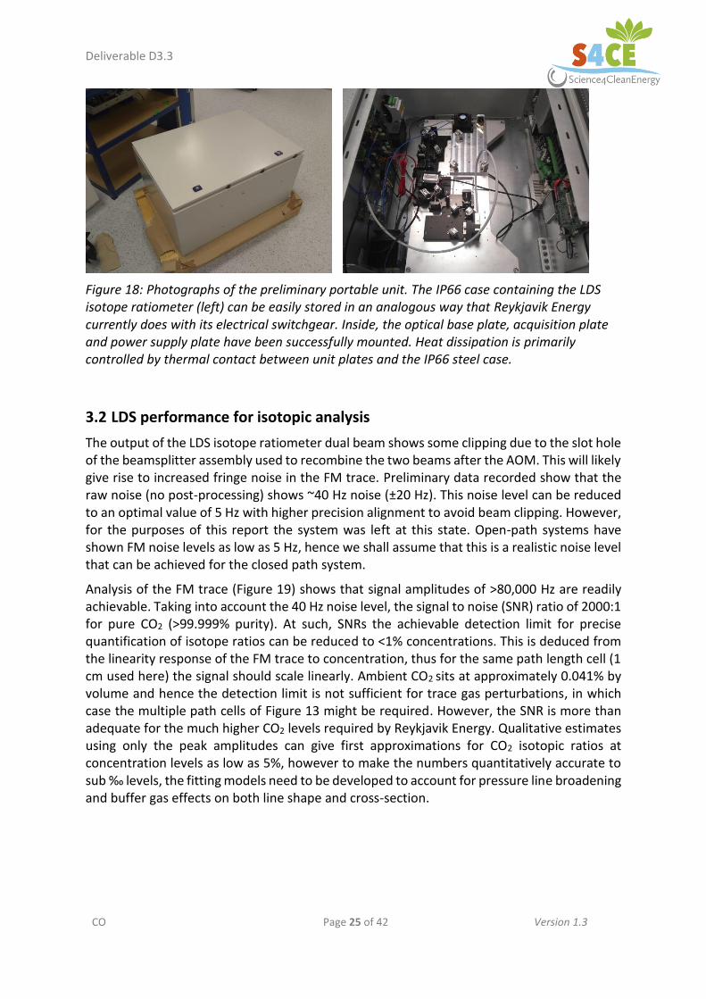
Figure 18: Photographs of the preliminary portable unit. The IP66 case containing the LDS isotope ratiometer (left) can be easily stored in an analogous way that Reykjavik Energy currently does with its electrical switchgear. Inside, the optical base plate, acquisition plate and power supply plate have been successfully mounted. Heat dissipation is primarily controlled by thermal contact between unit plates and the IP66 steel case.

3.2 LDS performance for isotopic analysis

The output of the LDS isotope ratiometer dual beam shows some clipping due to the slot hole of the beamsplitter assembly used to recombine the two beams after the AOM. This will likely give rise to increased fringe noise in the FM trace. Preliminary data recorded show that the raw noise (no post-processing) shows ~40 Hz noise (±20 Hz). This noise level can be reduced to an optimal value of 5 Hz with higher precision alignment to avoid beam clipping. However, for the purposes of this report the system was left at this state. Open-path systems have shown FM noise levels as low as 5 Hz, hence we shall assume that this is a realistic noise level that can be achieved for the closed path system.

Analysis of the FM trace (Figure 19) shows that signal amplitudes of >80,000 Hz are readily achievable. Taking into account the 40 Hz noise level, the signal to noise (SNR) ratio of 2000:1 for pure CO2 (>99.999% purity). At such, SNRs the achievable detection limit for precise quantification of isotope ratios can be reduced to <1% concentrations. This is deduced from the linearity response of the FM trace to concentration, thus for the same path length cell (1 cm used here) the signal should scale linearly. Ambient CO2 sits at approximately 0.041% by volume and hence the detection limit is not sufficient for trace gas perturbations, in which case the multiple path cells of Figure 13 might be required. However, the SNR is more than adequate for the much higher CO2 levels required by Reykjavik Energy. Qualitative estimates using only the peak amplitudes can give first approximations for CO2 isotopic ratios at concentration levels as low as 5%, however to make the numbers quantitatively accurate to sub ‰ levels, the fitting models need to be developed to account for pressure line broadening and buffer gas effects on both line shape and cross-section.

Deliverable D3.3


Figure 19: FM signal acquired for industrial grade (99.999%) CO2 at ~40 Torr in the static gas cell. The FM trace demonstrates substantial signal as expected under the current experimental conditions. The larger peak (centred at 475) is a 12C dispersion signal and the smaller peak (centred at 725) is the 13C dispersion signal of interest. The signal is duplicated/mirrored after data point 810 as the LDS measurement includes a reverse scan of the laser current, and thus a reverse wavelength scan.

These results compare favourably with the preliminary results using 5% CO2 obtained for the laboratory setup reported in January 2019, which is reproduced in Figure 20. We observe some modest improvement in the baseline noise (see Figure 20), but in both cases this excess noise stems from residual standing waves introduced by partial reflectors in the optical path.

Figure 19: Bench top laboratory setup for laser isotope ratiometer studies.

Deliverable D3.3


Figure 20: Isotopic optical dispersion signatures: Left, top panel, raw FM signal showing the molecular dispersion of CO2 isotopologues ; Lower panel, two subsequent spectra subtracted showing an estimate of the fundamental noise affecting the spectrometer. Right, molecular spectrum with fit (top panel) and residual (bottom panel).

Using both the table top prototype and the field prototype, measurement of the FM signal of the ambient background showed a significant level of CO2 dispersion signal in the trace, up to 100 Hz at the peak positions of interest (see Figure 21 for the case of the field prototype). This can be accommodated for in the longer run by use of an active instrument/cell compartment purge with pure nitrogen to further reduce ambient CO2 levels. This will be needed for increasing the quantitative accuracy of the isotope measurement in the long run and is included in the longer-term March 2020 trial test. The site(s) of the trial will have a dry nitrogen source for purging, or alternatively a CO2 scrubbed stream of compressed air can be used. In addition to the ambient background, a Germanium etalon measurement was recorded; the results are plotted in Figure 22. The etalon trace is not only essential in calibrating the instrument wavenumber scale (relative or absolute if a standard signal is known – not shown) it is also useful highlighting if there are any issues with the instrument. From the data, it is clear to see two unusual behaviours in the data recorded. First, the etalon data shows a distinct distortion at the data point ranges 0-125 and 810-900. This is expected at the 810-900 region as this is when the current ramp changes direction from “forward” to “reverse”. The transient ramp rate differential gives rise to the distorted shape. What is less expected is the distortion at 0-125, the initial part of the forward scan. An investigation into the application of the laser current ramp will be required to reduce or remove this artefact. Despite that, there is still a lot of current ramp free data between these specified regions. The second artifact is a symmetric “drift” in the data seen in all three plots but in slightly different ways. The AM and phase plots show a drift of the average value to slightly higher values going from 0-850 and 850-1600. There is also a minor modulation to the signal amplitude going across the data point ranges. In the FM trace however, the average FM value (averaged over data point interval) still tends around 0 Hz as expected but the signal amplitude increases going from lower to higher data point values. Similar drifts have been observed when the path length difference between the zero and first order beams is not close to 0, such as ~10’s of μm. This is discussed in the later in this report. However, it is quite pronounced and does not follow the exact same symmetric pattern as previously seen. This effect has to be considered when discussing the relative CO2 peak amplitudes as it is likely to be an underlying artifact in the data. As mentioned previously, an offset in the path lengths is the most likely candidate

Deliverable D3.3


to check for this distortion in the etalon signature, but in addition the AOM beam diffraction should be checked to ensure that the beam intensities are balanced. Another possibility is the calibration of the chirp rate. A significantly nonlinear chirp rate might give rise to such signal drifts as observed here. A final source of error could be an asymmetric clipping of the beam. This was observed to be an unfortunate error in the initial alignment of the system at the beamsplitter, where the zeroth order beam was partially clipped by the edge of the beam port. Systematic alignment while checking beam profile and etalon dispersion signal can be used to check if this plays a role in the signal drift observed.

Figure 21: FM signal acquired for the ambient air in the instrument. Total signal amplitude is up to 100 Hz. This additional signal effectively lowers the real signal to noise ratio to <1000:1, removing the ability to do sub % isotopic ratio measurements. Inert gas purging will minimize this contribution to within the intrinsic instrument detection limits (sub Hz).

The final test conducted was a simple wavelength scan of the CO2 sample by shifting the temperature of the laser head to alter the emission wavelength. Computation of the absorption cross section for a pure CO2 sample at 40 Torr, 295 K and use of a 1 cm path length cell was conducted using the publicly available HITRAN web service.[8] The results for CO2 containing natural abundance of 12C and 13C is given (Figure 23, panel a). Calculations using 14C were performed but no significant transitions were predicted to occur in this region. Using the HITRAN results as a reference the laser head temperature was tuned from 16.6 °C to 4.1 °C giving an approximate scan range of 3 cm-1 (using a ±7 mA scan around the set laser current) which corresponds to an effective scan from 2295 cm-1 to 2298 cm-1. The FM traces were recorded, and the patterns were matched with the HITRAN data (see Figures 23, panels b-g). Note, that the FM plots have a flipped x-axis, and that this is to match the wavenumber axis direction of the HITRAN data or i.e. place both sets of data the right way around. Considering the amplitude drift observed in the etalon data, there is a good qualitative match of the FM signal amplitudes and the HITRAN data. The number of transitions (and the pattern) observed also match very well with the HITRAN calculations.

Deliverable D3.3


Figure 22: Measurements of a Germanium substrate to give an adequate etalon signal. The AM, FM and phase signals are given in the top, middle and bottom plots, respectively. All plots show a “drift” in the etalon trace indicating an alignment mismatch either in the delay line path length (likely) or possibly in the AOM beam intensity balance (unlikely). There is also a distortion in the trace between data points 0-125. This region is at the start of the laser current forward ramp and has been noted to affect the signal amplitude, especially in the FM trace for pure CO2. This is likely due to a transient change in the current ramp rate as a similar distortion occurs at the centre of the plot around 810-900 data points in. This is when the current ramp changes direction and is known to always occur. Therefore, clean data can be taken in the ranges of 130-800 and 910-1620.

Deliverable D3.3


Figure 23: (a) Computed absorption cross sections for 12C and 13C based CO2 vibrational transitions using the HITRAN online package. The plot has been labelled qualitatively to match theoretical spectrum region with experimentally measured region from the isotope ratiometer (b-g).

3.3 Sample cell design: static and multipass

3.3.1 3.3.0 Manufacture of multifaceted multipass cells

The multifaceted mirrors are produced by specialist diamond tool machining, which must produce very high-quality optical surfaces to minimize scattering losses (and optical interference noise). Although the mirrors are gold coated for high reflectivity in the mid infrared, the substrate quality produced by the machining is critical to the overall quality. The larger facet number mirrors e.g. 8x6 were produced by Nanophorm LLC and Son-X GmBh and the supply of these took much longer than expected leading to project delays. These multifaceted mirrors arrived in May 2019 and the MFM cell was built as shown in Figure 24. The small number facet mirrors for the short optical path length MFM cell was produced by the STFC facilities and this is shown in Figure 25.

Deliverable D3.3


Figure 24: Left: Bench top setup of long optical path MFM multipass cell. Right: with gas cell enclosure installed.

Figure 25: Short optical path (1.97m) MFM multipass cell corresponding to the design shown in Figure 13.

Analysis of the mirror surface quality was performed using a digitally assisted microscope (Keyence Ltd) and white light interferometer (Zygo) which allows defects in the mirror facets to be observed in detail. One example for a single mirror facet on the SON-X part is shown in Figure 26 shows a digital image analysis by the microscope software, in which the histogram shows that the majority of defects are between 1 to 2 micron in size. Although they are smaller than the mid infrared wavelengths for which the mirror is used, they can still contribute to scattering and reflection losses. In Figure 27 a result from the white light interferometer is shown showing the surface roughness on a Nanophorm MFM facet. Other analyses were also performed to investigate the individual facet ROC, tilt angles, overall transmission, mechanical tolerance and optical noise.

Deliverable D3.3


Figure 26: Left: Zoom of mirror facet defects. Right: digital image analysis of defects.

Figure 27: Screenshot of the surface quality evaluation by a Zygo white light interferometer as obtained from nanophorm. The regular vertical striation observed by the microscope could correspond to the blue lines in the graph in the upper middle panel. It should be noted, that the area probed is rather small in comparison to the overall facet size.

3.3.2 Modelling of beam propagation in the short OPL multipass cell

Figure 28 shows the beam propagation model of a configuration for forming a beam waist at the multipass cell plane mirror with acceptable beam diameters at the entrance and exit windows. This model allowed the validation of the beam properties observed with the actual cell and the preparation of integration into the rest of the optical head of the instrument.

Deliverable D3.3


Figure 28: Beam propagation model for incorporation of multipass cell into the existing laser/AOM configuration

3.3.3 Multipass cell hermeticity

The seal between cell and mirror end-caps was made using CS nitrile O-rings of nominal diameter 20.5 mm (Polymax, P/N 20.5X1N70). The cell was connected to a vacuum line using Clippard PQ-CC045 push-fit connectors (M5 thread, 1/8” OD tube).

Problems were observed with regards to the leak rate of the cell, arising from material contact mismatch. The leak rate of all vacuum line components except the cell was measured as 8 Torr in 15 hours into 12 cm3, corresponding to a mass flow of 1.4 x 10-4 sccm. The leak rate of the vacuum system incorporating the cell was found to be 45 Torr in 1 min into 27 cm3 corresponding to a mass flow of 1.5 sccm.

Figure 29: Microscope images of the Al-acrylic interface illustrating channels in bonding

Deliverable D3.3


In Figure 29 we report microscope images of the edge of the cell channel – the aluminium base in the upper part, the channel in the lower. The left-hand image shows bubbles apparent where the Al-acrylic interface meets the channel. Some of these bubbles were seen to be moving when the cell was under vacuum – this is not a static structure. The right-hand image shows channels & pockets apparent in the interface between the Al block and the acrylic, possibly caused by outgassing or an originally imperfect bond between substrates.

On closer inspection, there appeared to be fluid remaining in the cell, most likely being machining fluid from PDF milling machines, so the cell was dismantled and rinsed in isopropanol, following which the leak rate was measured to be 37 Torr in 1 min. On pumping immediately after the isopropanol rinse, fluid could be seen running along some channels in the interface into the cell.

The observed pressure increase would correspond to an outgassing rate constant of 4.5 x 10-

4 Torr.l.s-1.cm-2 if due to outgassing of the Perspex. For future versions of this instrument, materials such as polycarbonate (Lexan) could be considered as they provide much lower outgassing rates (~ 5 x 10-7 Torr.l.s-1.cm-2).

One longitudinal seam was sealed with Araldite with the cell under vacuum. Following overnight cure, the leak rate was measured to be 38 Torr in 1 min. The other seam was then also sealed and pumped for 24 hours, following which the leak rate was measured at 48 Torr in 1 min.

Possible remaining sources of leak are:

polymer-Al interface at ends of cell

cracks in polymer at end-cap screw threads which would be difficult to seal.

Some further design shortcomings include:

potential shear force along Perspex-aluminium interface generated by end-cap mounting screws

potential step in O-ring groove at Perspex-Al interface

An alternative solution is to operate the cell in flow mode using a simple LabVIEW VI to control Bronkhorst pressure and flow controllers. A flow of 150 sccm 5 % CO2 would be sufficient to keep impurities form leak or outgassing to the 1 % level.

3.3.4 Preparation of static pure CO2 samples: sealed static cells

As the field demonstration will in fact be carried out on near-pure CO2, a mitigation for the lack of a hermetic flow cell would be to use existing 1-cm sealed glass cells with a static CO2 sample. Three cells, numbered 2, 4 and 5 were available and were leak-tested against the base leak rate of a vacuum system.

Figure 30 compares the leak rates of the three cells to the vacuum system base leak rate. The leak rates of the vacuum system and cells 2 and 5 show an initial rise of ~ 8 Torr over ~ 30 hours, which is interpreted as outgassing, followed by a slower steady rise of ~ 10 Torr over ~

Deliverable D3.3


200 hours taken to represent a true leak rate. The similarity in behaviour of the cells compared to the isolated vacuum system suggests that the observed leak rate is dominated by the vacuum system and places an upper limit on the cell leak rate of ~ 30 mTorr.hour-1. Cell 4 as first tested clearly suffers from a major leak; following treatment of the window seals between window and cell, however, its leak rate was found to be commensurate with the base leak rate.

Figure 30: Leak rates of the vacuum system and cells

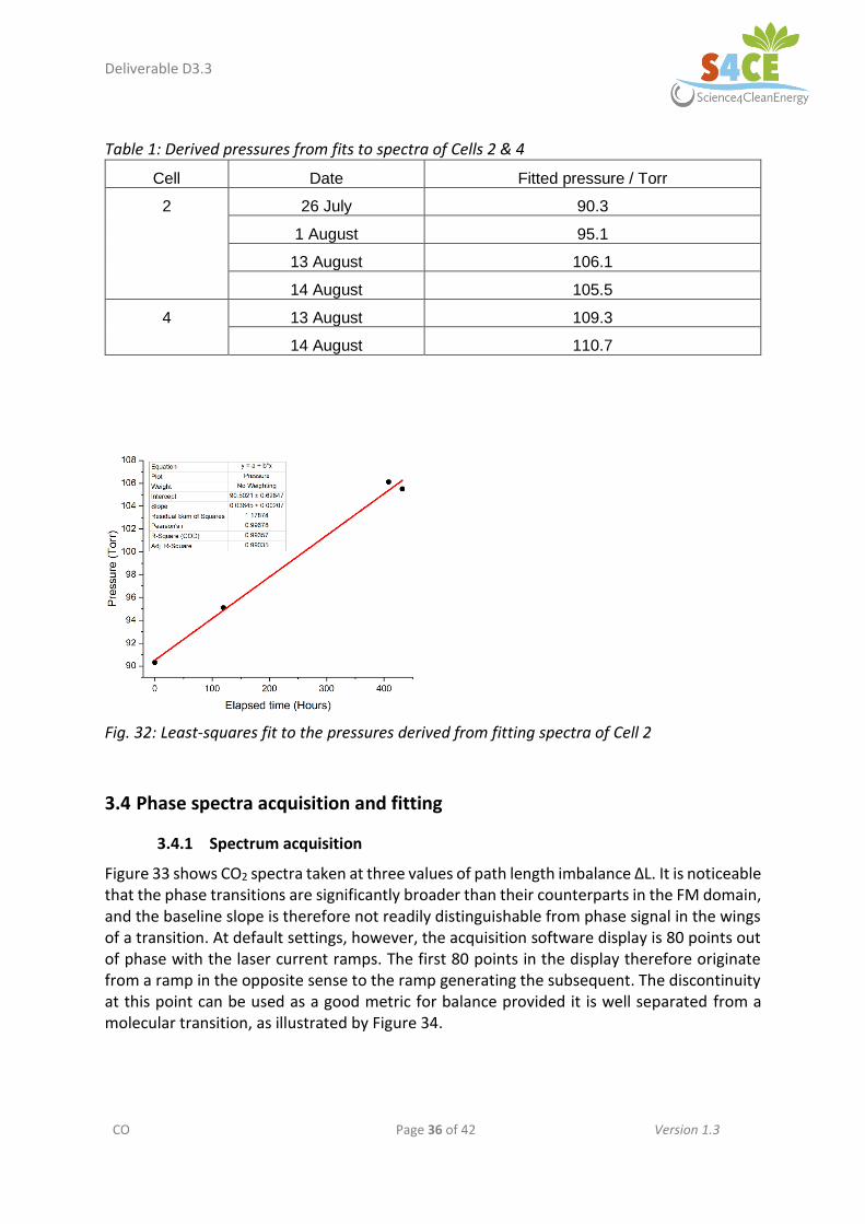
Cells 2 and 4 were filled with 100 ± 1 Torr pure CO2 and sealed by melting off and collapsing the cell stem as shown in Figure 30. Spectra of Cell 2 were measured periodically to assess the leak rate. A spectrum of cell 4, sealed later, was recorded for reference. Figure 31 shows the spectra of the 2296.056 cm-1 12CO2 line, aligned in wavenumber for comparison. Cell pressures for derived from the fit procedure described in section 6 are listed in Table 1. Statistical errors returned from the fit are ~ 0.01 Torr, but these are unrealistically small in the light of the large model error described in Section 3.4.2. Figure 32 shows the linear fit to the data for Cell 2, which indicates a leak rate of ~ 35 mTorr.hr-1.

Figure 31: Spectra of Cells 2 & 4 at intervals after filling

Deliverable D3.3


Table 1: Derived pressures from fits to spectra of Cells 2 & 4

Cell Date Fitted pressure / Torr

2 26 July 90.3

1 August 95.1

13 August 106.1

14 August 105.5

4 13 August 109.3

14 August 110.7

Fig. 32: Least-squares fit to the pressures derived from fitting spectra of Cell 2

3.4 Phase spectra acquisition and fitting

3.4.1 Spectrum acquisition

Figure 33 shows CO2 spectra taken at three values of path length imbalance ΔL. It is noticeable that the phase transitions are significantly broader than their counterparts in the FM domain, and the baseline slope is therefore not readily distinguishable from phase signal in the wings of a transition. At default settings, however, the acquisition software display is 80 points out of phase with the laser current ramps. The first 80 points in the display therefore originate from a ramp in the opposite sense to the ramp generating the subsequent. The discontinuity at this point can be used as a good metric for balance provided it is well separated from a molecular transition, as illustrated by Figure 34.

Deliverable D3.3


Figure 33: CO2 spectra (100 Torr, 1 cm path length) taken at three values of path length imbalance ΔL.

Figure 34: Use of phase signal at the laser ramp discontinuity to achieve balancing.

So far, frequency calibration was carried out using the AM demodulated spectrum of an etalon of known free spectral range (FSR). Owing to the known susceptibility of the detector signal to optical feedback in the optical chain, such AM etalon signals often show significant distortion. Even with care in positioning the etalon, residual distortion can remain such as the asymmetric fringes shown in Figure 34. Compared to the AM signal, the phase signal shows both a more uniform amplitude and more symmetric fringe structure. For the scopes of the present Deliverable, therefore, frequency calibration was performed using etalon phase spectra (see Figure 35).

Deliverable D3.3


Figure 35: Comparison of a CO2 spectrum with the AM and phase spectrum of the etalon used for frequency calibration.

3.4.2 Phase forward model

The main feature of the forward model is the expression of the total demodulated phase Φ(t) in to three separate components φω(t), φL(t) and φn(t). The term φω(t) is driven primarily by the 200 MHz frequency difference between the zeroth and first order beams. The term φL(t) is driven by the length and composition of the free space propagation paths of the two beams. The term φn(t) is sensitive to the refractive index of the sample. All three terms contain a contribution from the path length imbalance ΔL of the two beams, which has the effect of introducing both an offset and a slope to the spectrum baseline.

A further feature is the derivation of a time-dependent chirp rate to replace of the assumption of constant value. Frequency calibration is performed by determining the index positions, n, of peaks and troughs in the etalon trace and associating a relative wavenumber ν _̅rel to each successive index given by the FSR of the etalon. Fitting the optimum polynomial P of order up to 8 and converting index to time gives a parameterization ν ̅_rel(t) = P(t), from which the chirp rate S(t) is extracted by differentiation : S(t) = P'(t). Typical results are shown in Fig. 36.

Figure 36: Relative wavenumber and corresponding chirp rate extracted from a typical etalon trace.

Deliverable D3.3


3.4.3 Fitting with the phase forward model

A number of shortcomings or limitations in the initial formulation of the forward model for fitting purposes were found, as described as follows.

Line position mismatch between data and forward model

Fitting of data is performed using the wavenumber calibration as described above with the introduction of a central wavenumber as a fit parameter. A slight mismatch in separation of the principal 12CO2 and 13CO2 lines of ~ 1.5 % was found between data and model, shown in Figure 37.

Figure 37: Matching the 12CO2 and 13CO2 transitions using a scaling parameter (30 Torr 5% CO2 in N2)

The reason for the mismatch has not yet been established. The two HITRAN transitions at 2295.8456 and 2296.05639 cm-1 have separation 0.210769 cm-1. The uncertainty on each line position is HITRAN level 4, corresponding to 0.0001-0.001 cm-1. The maximum 1-σ uncertainty on the line separation is therefore 0.0014 cm-1, whereas the separation according to the etalon calibration is 0.20728 cm-1, 0.00349 cm-1 smaller than the HITRAN value. For this work the mismatch was addressed using an empirical scaling factor on the time axis as a fitting parameter.

Convergence problems

Fits using the original 3-component phase model showed good convergence for the central wavenumber parameter provided the a priori estimate is within ~ 0.05 cm-1 of the optimum. Convergence for all other parameters was poor. Simulations using the 3-component phase model show that quite subtle changes in spectrum baseline slope generated by changes in ΔL are accompanied by large changes in baseline offset. The effect is illustrated in Figure 38, which shows simulations performed for ΔL in the range 0-1000 µm. The spectra in the right-hand plot have been pinned to zero phase at 200 µs to illustrate the change in baseline slope. To test the possibility that baseline-slope correlations may impede convergence, a step was included in the forward model to reduce the spectra to zero-mean to reflect that fact that spectra returned by the acquisition software have a range –π to π. Convergence nonetheless remained poor.

Deliverable D3.3


Figure 38: Simulations illustrating the combined effect on slope and offset of varying path imbalance.

A further modification was made to the forward model, in which the phase terms φω(t) and φL(t), which contribute only to the baseline, were replaced by an empirical quadratic around the mid-point of the time axis; convergence was significantly improved as a result. It is possible that a revised forward model using reformulation of the expressions for φω(t) and φL(t) may show better convergence behavior, but for present purposes the empirical quadratic baseline model was used for all further fitting.

Instrument response function

The forward model initially modelled the demodulation response function (ILS) as a digital filter (Nyquist 468.75 kHz, filter power 75, number of filter elements 2.5% the size of the time vector). The true ILS was measured for a range of filer bandwidths by applying a phase delta function to the demodulator input. The resulting ILS functions are shown in Figure 39, which also compares the experimentally determined ILS for 400 kHz with the corresponding digital filter. The experimentally determined function was subsequently used for the forward model.

Figure 39: Digital filter ILS (left) and the experimentally determined ILS for 400 kHz BW (right) compared to its digital counterpart

Deliverable D3.3


Residuals

Despite the improvement in convergence achieved using the quadratic baseline and the inclusion of the ILS, fit residuals suggest that there remains a significant source of model error. Figure 40 represents the best fit achieved, including just the 12C and 13C isotopomers and constraining their concentrations to the natural abundance of 0.998.

The errors on the relevant HITRAN broadening parameters are low (confidence level 7 corresponds to an error of 1-2 %) and are therefore unlikely to be the sole source of error. Detailed investigation of the lineshape model error is outside project scope, but given that the samples are pure CO2, future work should examine carefully the validity of the currently assumed Voigt lineshape model for self-broadening of CO2.

Figure 40: Optimum fit and residuals for a 1-cm path length of 100 Torr pure CO2

4 Conclusions and future steps

To summarize this report, a working prototype for a spectroscopic isotope ratiometer using the laser dispersion spectroscopic method developed and pioneered into commercialization by MIRICO. The design is simple yet robust, incorporates most of the main aspects and utilizes the existing technology for the ORION open path LDS system that MIRICO has developed for commercial scale trials and sales. There are still improvements needed with regards to appropriate installation of the network communication hubs inside the box and the development of the extractive gas sample cell and gas flow control system necessary for the March 2020 trials. However, the project remains on schedule and all remaining improvements/missing components can be completed before the field trial. The prototype instrument demonstrates a sufficient signal to noise ratio for quantitative analysis at the few % level (1-5%) and possibly at sub 1% levels. Improvements in system alignment should yield a 5-fold or greater improvement in reducing the background instrument noise. Some further development is required to enhance the instrument ability to fit the isotope peaks, and initial steps are underway to improve software and data-processing capabilities.

In addition, significant developmental work was done producing a long optical path compact multipass cell based on a novel multifaceted mirror approach, which could be useful when applications might require sensitivity enhancement.

Deliverable D3.3


5 Bibliographical references

[1] Carbfix, Carbfix: Our Story, Available at: https://www.mendeley.com/guides/web-citation-guide (Accessed at: 19 August 2019)

[2] S. R. Gislason et. al., Int. J. Greenh. Gas. Con, 2010, 4, 537-545

[3] J. M. Matter et. al., Science, 2016, 352, 1312-1314

[4] S. Ó. Snæbjörnsdóttir et. al., Int. J. Greenh. Gas. Cont, 2017, 58, 87-102

[5] S. R. Gislason et. al., Geochim. Cosmochim. Ac, 2018, 245, 542-555

[6] G. Wysocki, D. Weidmann., Opt. Exp, 2010, 18, 26123-26140

[7] N. S. Daghestani, R. Brownsword, D. Weidmann, Opt. Exp, 2014, 22, A1731-A1743

[8] HITRAN, HITRAN on the Web, Available at: http://hitran.iao.ru/bands/simlaunch (Accessed at: 19th August 2019)

[9] D. Weidmann, C.B. Roller, C. Oppenheimer, A. Fried, and F.K. Tittel, Isotopes in Environmental and Health Studies 41, 2005, 4, 293-302

https://www.mendeley.com/guides/web-citation-guide

https://www.mendeley.com/guides/web-citation-guide

http://hitran.iao.ru/bands/simlaunch

Date post:	21-Oct-2021
Category:	Documents
Upload:	others
View:	0 times
Download:	0 times

Science for Clean Energy

Documents