Scilab Code for Elements of chemical Reaction Engineering by H. Scott Fogler 1 Created by Santosh Kumar Dual Degree student B. tech + M. Tech (Chem. Engg.) Indian Institute of Technology, Bombay College Teacher and Reviewer Arun Sadashio Moharir Professor IIT Bombay IIT Bombay 17 October 2010 1 Funded by a grant from the National Mission on Education through ICT, http://spoken-tutorial.org/NMEICT-Intro.This text book companion and Scilab codes written in it can be downloaded from the ”Textbook Companion Project” Section at the website http://scilab.in/
Transcript
Scilab Code forElements of chemical Reaction Engineering
by H. Scott Fogler1
Created bySantosh Kumar
Dual Degree studentB. tech + M. Tech (Chem. Engg.)
Indian Institute of Technology, Bombay
College Teacher and ReviewerArun Sadashio MoharirProfessor IIT Bombay
IIT Bombay
17 October 2010
1Funded by a grant from the National Mission on Education through ICT,http://spoken-tutorial.org/NMEICT-Intro.This text book companion and Scilabcodes written in it can be downloaded from the ”Textbook Companion Project”Section at the website http://scilab.in/
Book Details
Author: H. Scott Fogler
Title: Elements of chemical Reaction Engineering
Publisher: Prentice-Hall International, Inc., New Jersey
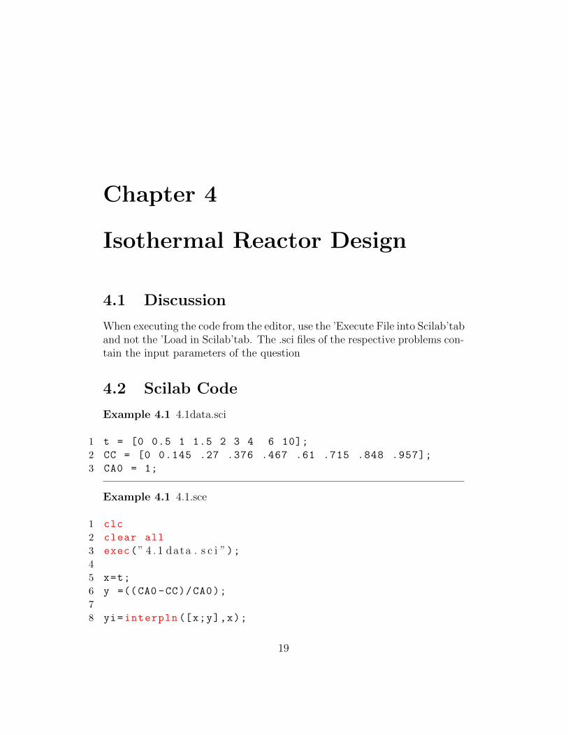
When executing the code from the editor, use the ’Execute File into Scilab’taband not the ’Load in Scilab’tab. The .sci files of the respective problems con-tain the input parameters of the question
1.2 Scilab Code
Example 1.3 1.3data.sci
1 k = 0.23; // minˆ−12 v0 = 10; //dmˆ3/ min
Example 1.3 1.3.sce
1 clc
2 clear all
3 exec(” 1 . 3 data . s c i ”);4
5 //CA = 0 . 1∗CA0 ;6 V = (v0/k)*log (1/0.1);
7 disp(”V =”)8 disp(V)
9 disp (”dmˆ3 ”)
9
10
Chapter 2
Conversion and Reactor Sizing
2.1 Discussion
When executing the code from the editor, use the ’Execute File into Scilab’taband not the ’Load in Scilab’tab. The .sci files of the respective problems con-tain the input parameters of the question
2.2 Scilab Code
Example 2.1 2.1data.sci
1 P0 = 10; //atm2 yA0 = 0.5;
3 T0 = 422.2; //K4 R = 0.082; // dmˆ 3 . atm/mol .K5 v0 = 6; //dmˆ3/ s
Example 2.1 2.1.sce
1 clc
2 clear all
3 exec(” 2 . 1 data . s c i ”);4 CA0=(yA0*P0)/(R*T0);
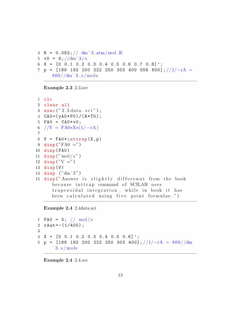
7 p = [189 192 200 222 250 303 400 556 800]; //1/−rA =800//dmˆ 3 . s / mols
Example 2.3 2.3.sce
1 clc
2 clear all
3 exec(” 2 . 3 data . s c i ”);4 CA0=(yA0*P0)/(R*T0);
5 FA0 = CA0*v0;
6 //V = FA0∗X∗(1/−rA )7
8 V = FA0*inttrap(X,p)
9 disp(”FA0 =”)10 disp(FA0)
11 disp(”mol/ s ”)12 disp(”V =”)13 disp(V)
14 disp (”dmˆ3 ”)15 disp(” Answer i s s l i g h t l y d i f f e r e n n t from the book
because i n t t r a p command o f SCILAB u s e st r a p e z o i d a l i n t e g r a t i o n , w h i l e i n book i t hasbeen c a l c u l a t e d u s i n g f i v e p o i n t f o rmu la e . ”)
Example 2.4 2.4data.sci
1 FA0 = 5; // mol/ s2 rAat = -(1/400);
3
4 X = [0 0.1 0.2 0.3 0.4 0.5 0.6]’;
5 p = [189 192 200 222 250 303 400]; //1/−rA = 800//dmˆ 3 . s / mols
3 p = [189 192 200 222 250 303 400 556 800]; //1/−rA =800//dmˆ 3 . s / mols
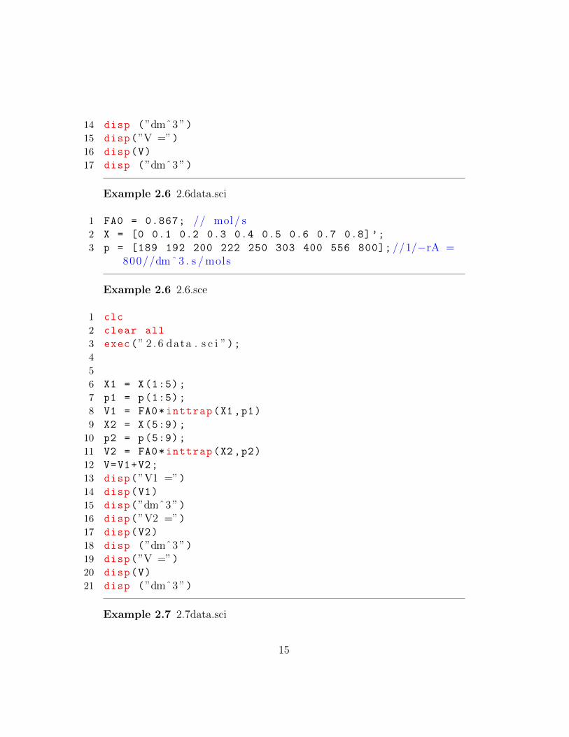
Example 2.6 2.6.sce
1 clc
2 clear all
3 exec(” 2 . 6 data . s c i ”);4
5
6 X1 = X(1:5);
7 p1 = p(1:5);
8 V1 = FA0*inttrap(X1,p1)
9 X2 = X(5:9);
10 p2 = p(5:9);
11 V2 = FA0*inttrap(X2,p2)
12 V=V1+V2;
13 disp(”V1 =”)14 disp(V1)
15 disp(”dmˆ3 ”)16 disp(”V2 =”)17 disp(V2)
18 disp (”dmˆ3 ”)19 disp(”V =”)20 disp(V)
21 disp (”dmˆ3 ”)
Example 2.7 2.7data.sci
15
1 FA0 = 0.867; // mol/ s2 X1 = 0.5;
3 X2 = 0.8;
4 rA2 = -(1/800);
5 X = [0 0.1 0.2 0.3 0.4 0.5 0.6 0.7 0.8]’;
6 p = [189 192 200 222 250 303 400 556 800]; //1/−rA =800//dmˆ 3 . s / mols
Example 2.7 2.7.sce
1 clc
2 clear all
3 exec(” 2 . 7 data . s c i ”);4
5
6 X = X(1:6);
7 p = p(1:6);
8 V1 = FA0*inttrap(X,p);
9 V2 = FA0*(X2 -X1)*(1/-rA2);
10 V=V1+V2;
11 disp(”V1 =”)12 disp(V1)
13 disp(”dmˆ3 ”)14 disp(”V2 =”)15 disp(V2)
16 disp (”dmˆ3 ”)17 disp(”V =”)18 disp(V)
19 disp (”dmˆ3 ”)
16
Chapter 3
Rate Laws and Stoichiometry
3.1 Discussion
When executing the code from the editor, use the ’Execute File into Scilab’taband not the ’Load in Scilab’tab. The .sci files of the respective problems con-tain the input parameters of the question
3.2 Scilab Code
Example 3.5 3.5data.sci
1 CA0 = 10;
2 CB0 = 2;
3 X = 0.2;
4 X1=0.9
Example 3.5 3.5.sce
1 clc
2 clear all
3 exec(” 3 . 5 data . s c i ”);4 CD=CA0*(X/3);
5 CB=CA0*(( CB0/CA0) -(X/3));
6 CD1=CA0*(X1/3);
7 CB1=CA0*((CB0/CA0)-(X1/3));
17
8 disp(” For 20% c o n v e r s i o n ”)9 disp(”CD =”)10 disp(CD)
11 disp (”mol/dmˆ3 ”)12 disp(”CB =”)13 disp(CB)
14 disp(”mol/dmˆ3 ”)15 disp(” For 90% c o n v e r s i o n ”)16 disp(”CD =”)17 disp(CD1)
18 disp (”mol/dmˆ3 ”)19 disp(”CB =”)20 disp(CB1)
21 disp(”mol/dmˆ3 ”)
18
Chapter 4
Isothermal Reactor Design
4.1 Discussion
When executing the code from the editor, use the ’Execute File into Scilab’taband not the ’Load in Scilab’tab. The .sci files of the respective problems con-tain the input parameters of the question
1 k = 0.311; // minˆ−1;2 FC= 6.137; // l b . mol/min3 X = 0.8;
4 CA01= 1; // mol/dmˆ3
Example 4.2 4.2.sce
1 clc
2 clear all
3 exec(” 4 . 2 data . s c i ”);4
5 FA0 = FC/X;
6 vA0 = FA0/CA01;
7 vB0 = vA0;
8 v0 = vA0+vB0;
9 V = v0*X/(k*(1-X));
10
11 // CSTR i n p a r a l l e l12 V1 = 800/7.48;
13
14 Tau =V1/(v0/2);
15 Da= Tau*k;
16 Xparallel = Da/(1+Da)
17
18 // CSTR i n s e r i e s19 Tau =V1/v0;
20 n=2;
21 Xseries = 1- (1/(1+ Tau*k)^n);
22
23 disp(” Reactor volume ”)24 disp(V)
25 disp (” f t ˆ3 ”)26 disp(”CSTR i n p a r a l l e l X =”)27 disp(Xparallel)
28 disp(”CSTR i n s e r i e s X =”)29 disp(Xseries)
Example 4.4 4.4data.sci
21
1 k1 = 0.072; // s ˆ−1;2 yA0 = 1;
3 P0= 6; //atm4 R = 0.73; // atm/ l b . mol . oR5 T0 = 1980; //oR6 T1 = 1000; //K7 T2 = 1100; // K8 e=1;
9 E = 82000; // c a l /g . mol10 FB= 0.34; // l b . mol/ s11 X = 0.8;
Example 4.4 4.4.sce
1 clc
2 clear all
3 exec(” 4 . 4 data . s c i ”);4
5 FA0 = FB/X;
6 CA0 = yA0*P0/(R*T0);
7 R = 1.987;
8 k2 = k1*exp((E/R)*((1/T1) -(1/T2)));
9 V =( FA0/(k2*CA0))*((1+e)*log(1/(1-X))-e*X);
10
11 disp(” Reactor volume ”)12 disp(V)
13 disp(” f t ˆ3 ”)
Example 4.5 4.5data.sci
1 Ac = 0.01414; // f t ˆ22 m = 104.4; // lbm/h3 mu = 0.0673; // lbm/ f t . h4 Dp = 0.0208; // f t5 gc = 4.17e8; // lbm . f t / l b f . hˆ26 phi = 0.45;
7 bita0 = bita0 /(144*14.7);//atm/ f t8 P = ((1 -(2* bita0*L/P0))^.5)*P0;
9 deltaP = P0 - P;
10
11 disp(” de l t aP ”)12 disp(deltaP)
13 disp(”atm”)
Example 4.6 4.6data.sci
1 k = 0.0141; // l b . mol/atm . l b ca t . h2 FA0 = 1.08; // l b . mol/h3 FB0 = 0.54; // l b . mol/h4 FI = 2.03; // l b . mol/h5 bita0 = 0.0775; // atm/ f t6 Ac = 0.01414; // f t ˆ27 phi = 0.45;
8 rhoc = 120; // l b c a t / f t ˆ39 P0 = 10; // atm
10 X = 0.6;
Example 4.6 4.6.sce
1 clc
2 clear all
3 exec(” 4 . 6 data . s c i ”);
23
4
5 FT0 = FA0+FB0+FI;
6 yA0 = FA0/FT0;
7 e = yA0*(1-.5 -1);
8 PA0 = yA0*P0;
9 kdes = k*PA0 *(1/2) ^(2/3);
10 alpha = 2*bita0 /(Ac*(1-phi)*rhoc*P0);
11 W = (1 - (1 -(3* alpha*FA0 /(2* kdes))*((1+e)*log(1/(1-X
))-e*X))^(2/3))/alpha;
12
13
14 disp(”W”)15 disp(W)
16 disp(” l b o f c a t a l y s t per tube ”)
Example 4.7 4.7data.sci
1 kprime = 0.0266; // l b . mol/atm . l b ca t . h2 alpha = 0.0166;
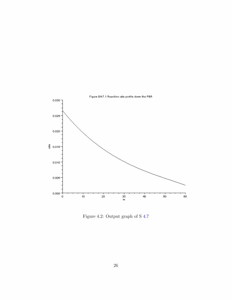
25 xtitle( ’ F i gu r e E4−7.1 Reac t i on r a t e p o r f i l e downthe PBR ’ , ’w ’ , ’ r a t e ’ ) ;
26 scf (2)
27
28 l1=x(1,: )’
29 l2=x(2,: )’
30 l3=F’
31 plot2d(W’,[l1 l2 l3]);
32
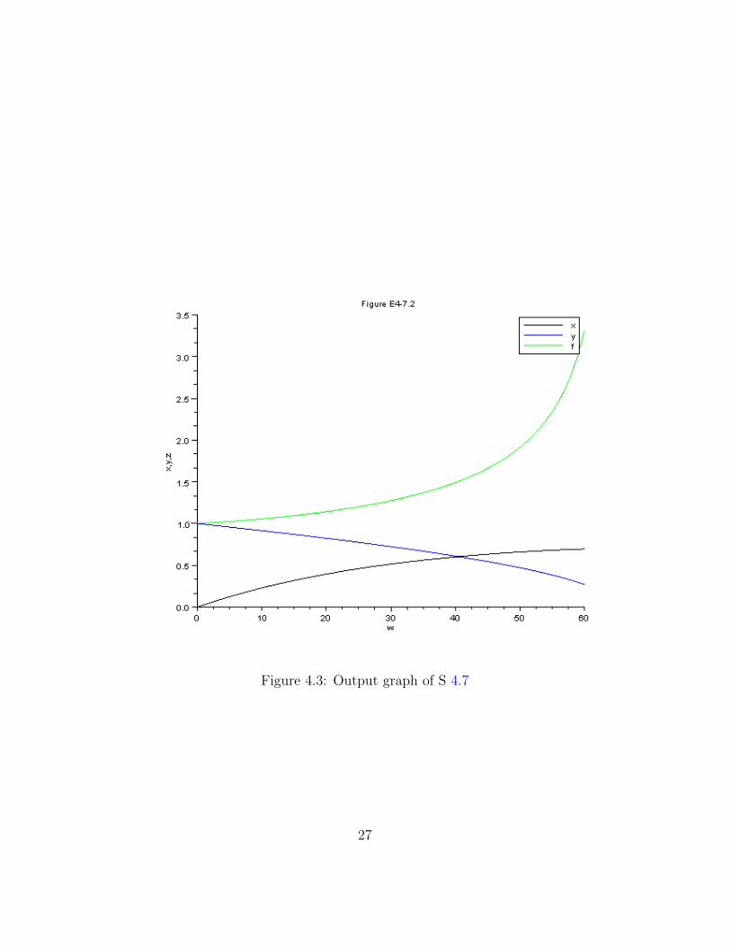
33 xtitle( ’ F i gu r e E4−7.2 ’ , ’w ’ , ’ x , y , z ’ ) ;
34 legend ([ ’ x ’ ; ’ y ’ ; ’ f ’ ]);
Example 4.8 4.8data.sci
1 FA0 = 440;
2 P0 = 2000;
3 Ca0 = .32;
4 R = 30;
5 phi = .4;
6 kprime = 0.02; // l b . mol/atm . l b ca t . h7 L = 27;
8 rhocat = 2.6;
9 m=44;
10
11 alpha = 0.0166;
25
Figure 4.2: Output graph of S 4.7
26
Figure 4.3: Output graph of S 4.7
27
12 e = -0.15;
13 Z0 = 0;
Example 4.8 4.8.sce
1 clc
2 clear all
3 exec(” 4 . 8 data . s c i ”);4 Z = 0:1:12;
5 function w=f(Z,Y)
6
7 w=zeros (2,1);
8 Ac= 3.14*((R^2) -(Z-L)^2);
9 Ca = Ca0*(1-Y(1))*Y(2) /(1+Y(1));
10 ra =kprime*Ca*rhocat *(1-phi);
11 G= m/Ac;
12 V =3.14*(Z*(R^2) -(1.3*(Z-L)^3) -(1/3)*L^3)
13 bita = (98.87*G+25630*G^2) *0.01;
14 W=rhocat *(1-phi)*V
15 w(1)= -ra*Ac/FA0
16 w(2) = -bita/P0/(Y(2) *(1+Y(1)));
17 endfunction
18
19
20 x=ode ([0;1] ,Z0 ,Z,f);
21 for i= 1: length(Z)
22 V(1,i) =3.14*Z(1,i)*((R^2) -(Z(1,i)-L)^2)
23 W1(1,i)=rhocat *(1-phi)*V(1,i)
24 end
25
26 l1=x(1,: )’
27 l2=x(2,: )’
28
29 plot2d(W1 ’,[l1 l2]);
30
31 xtitle( ’ F i gu r e E4−8.2 ’ , ’w ’ , ’ x , y ’ ) ;
32 legend ([ ’ x ’ ; ’ y ’ ]);
28
Figure 4.4: Output graph of S 4.8
29
Example 4.9 4.9data.sci
1 ka = 2.7;
2 kc = 1.2;
3 Ct0 = .1;
4 fa0 =10;
5 V0 = 0;
Example 4.9 4.9.sce
1 clc
2 clear all
3 exec(” 4 . 9 data . s c i ”);4 V = 0:1:100;
5 function w=f(V,fa)
6
7 w=zeros (1,1);
8 ft =2*(fa0 -fa(1))
9 Ca = Ct0*fa(1)/ft;
10 fb = 2*(fa0 -fa(1));
11 Cb = Ct0*fb/ft;
12 w(1)= -ka*(Ca -(Cb^2)/kc)
13
14 endfunction
15
16
17 x=ode ([9.99] ,V0 ,V,f);
18
19 for i= 1:101
20 fb(1,i) = 2*(fa0 -x(1,i));
21 end
22 l1=x’;
23 l2=fb ’;
24
25 plot2d(V’,[l1 l2]);
26
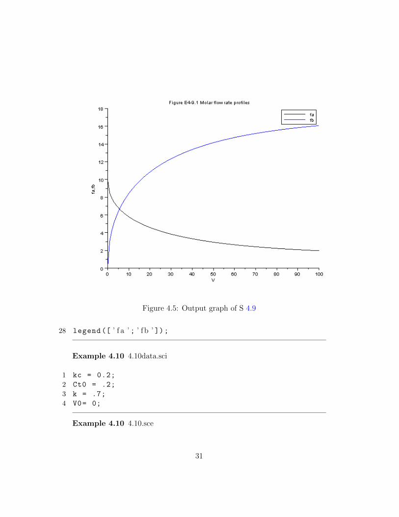
27 xtitle( ’ F i gu r e E4−9.1 Molar f l o w r a t e p r o f i l e s ’ , ’V’ , ’ fa , f b ’ ) ;
30
Figure 4.5: Output graph of S 4.9
28 legend ([ ’ f a ’ ; ’ f b ’ ]);
Example 4.10 4.10data.sci
1 kc = 0.2;
2 Ct0 = .2;
3 k = .7;
4 V0= 0;
Example 4.10 4.10.sce
31
1 clc
2 clear all
3 exec(” 4 . 1 0 data . s c i ”);4 V = 0:1:500;
5 function w=f(V,F)
6
7 w=zeros (3,1);
8
9 Ft=F(1)+F(2)+F(3);
10 ra = -k*Ct0 *((F(1)/Ft)-(Ct0/kc)*(F(2)/Ft)*(F(3)/Ft)
);
11 w(1)= ra;
12 w(2) = -ra-kc*Ct0*(F(2)/Ft)
13 w(3) = -ra;
14
15 endfunction
16
17
18 x=ode ([10;0;0] ,V0,V,f);
19
20 l1=x(1,: )’
21 l2=x(2,: )’
22 l3=x(3,: )’
23 plot2d(V’,[l1 l2 l3]);
24
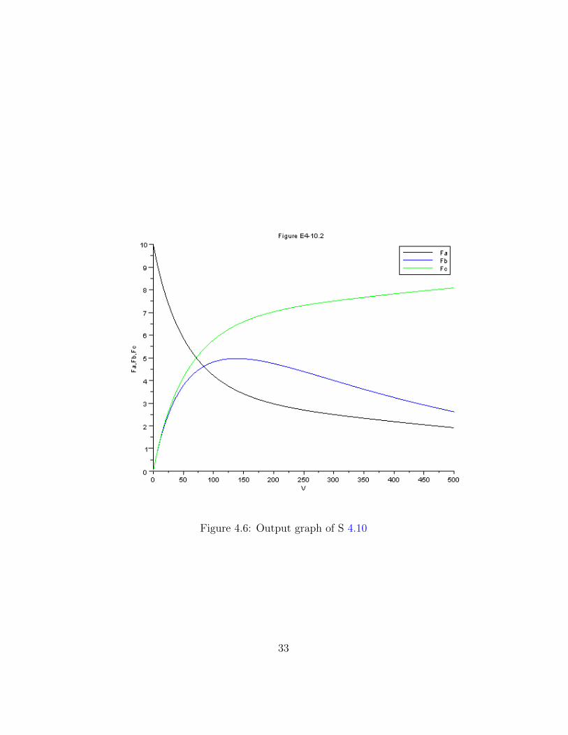
25 xtitle( ’ F i gu r e E4−10.2 ’ , ’V ’ , ’ Fa , Fb , Fc ’ ) ;
26 legend ([ ’ Fa ’ ; ’Fb ’ ; ’ Fc ’ ]);
Example 4.11 4.11data.sci
1 k= 2.2;
2 v00 = .05;
3 Cb0 = .025;
4 v0 = 5;
5 Ca0 = .05;
6 t0 = 0;
32
Figure 4.6: Output graph of S 4.10
33
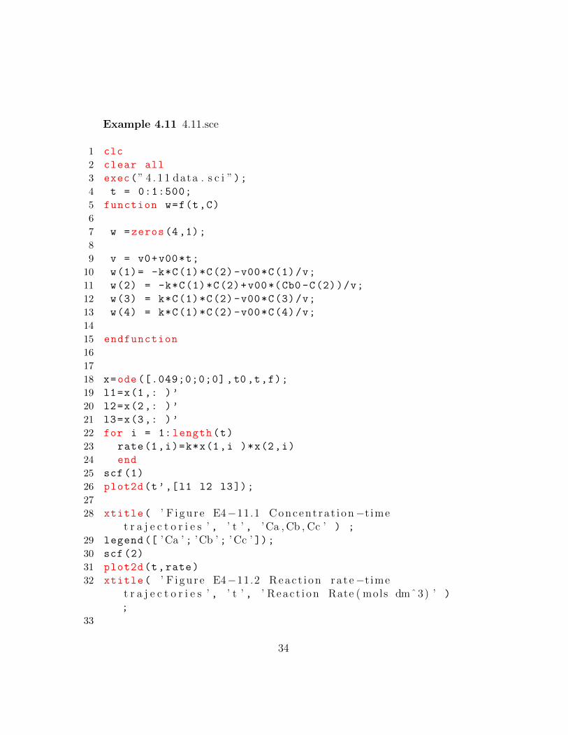
Example 4.11 4.11.sce
1 clc
2 clear all
3 exec(” 4 . 1 1 data . s c i ”);4 t = 0:1:500;
5 function w=f(t,C)
6
7 w =zeros (4,1);
8
9 v = v0+v00*t;
10 w(1)= -k*C(1)*C(2)-v00*C(1)/v;
11 w(2) = -k*C(1)*C(2)+v00*(Cb0 -C(2))/v;
12 w(3) = k*C(1)*C(2)-v00*C(3)/v;
13 w(4) = k*C(1)*C(2)-v00*C(4)/v;
14
15 endfunction
16
17
18 x=ode ([.049;0;0;0] ,t0,t,f);
19 l1=x(1,: )’
20 l2=x(2,: )’
21 l3=x(3,: )’
22 for i = 1: length(t)
23 rate(1,i)=k*x(1,i )*x(2,i)
24 end
25 scf (1)
26 plot2d(t’,[l1 l2 l3]);
27
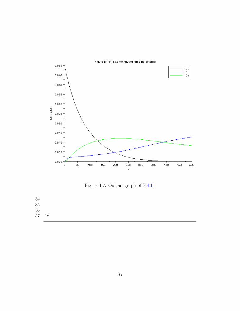
28 xtitle( ’ F i gu r e E4−11.1 Concent ra t i on−t imet r a j e c t o r i e s ’ , ’ t ’ , ’Ca , Cb , Cc ’ ) ;
29 legend ([ ’Ca ’ ; ’Cb ’ ; ’ Cc ’ ]);30 scf (2)
31 plot2d(t,rate)
32 xtitle( ’ F i gu r e E4−11.2 Reac t i on ra t e−t imet r a j e c t o r i e s ’ , ’ t ’ , ’ Reac t i on Rate ( mols dmˆ3) ’ )
;
33
34
Figure 4.7: Output graph of S 4.11
34
35
36
37 ’V
35
Figure 4.8: Output graph of S 4.11
36
Chapter 5
Collection and Analysis of RateData
5.1 Discussion
When executing the code from the editor, use the ’Execute File into Scilab’taband not the ’Load in Scilab’tab. The .sci files of the respective problems con-tain the input parameters of the question
5.2 Scilab Code
Example 5.2 5.2data.sci
1 t = [0 2.5 5 10 15 20]’;
2 P = [7.5 10.5 12.5 15.8 17.9 19.4] ’;
3 P0 = 7.5;
Example 5.2 5.2.sce
1 clc
2 clear all
3 exec(” 5 . 2 data . s c i ”);4 for i =1: length(t)
5 g(i) =log (2*P0/(3*P0 -P(i)));
6 end
37
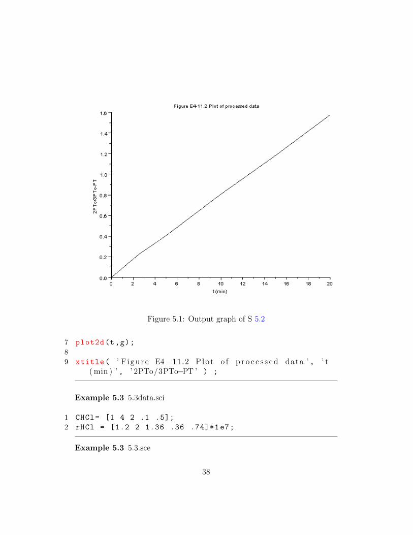
Figure 5.1: Output graph of S 5.2
7 plot2d(t,g);
8
9 xtitle( ’ F i gu r e E4−11.2 P lo t o f p r o c e s s e d data ’ , ’ t( min ) ’ , ’ 2PTo/3PTo−PT ’ ) ;
Example 5.3 5.3data.sci
1 CHCl= [1 4 2 .1 .5];
2 rHCl = [1.2 2 1.36 .36 .74]*1 e7;
Example 5.3 5.3.sce
38
1 clc
2 clear all
3 exec(” 5 . 3 data . s c i ”);4
5 x=log(CHCl);
6 y=log(-rHCl);
7 plot2d(x,y);
8
9 xtitle( ’ F i gu r e E5−3.2 ’ , ’CHCl ( g mol/ l i t e r ) ’ , ’rHCl0 ( g mol / cm ˆ 2 . s ) ’ ) ;
Example 5.4 5.4data.sci
1 CCH4 = [2.44 4.44 10 1.65 2.47 1.75] ’*1e-4;
2 PCO= [1 1.8 4.08 1 1 1]’;
3 v0 =300;
4 W= 10;
Example 5.4 5.4.sce
1 clc
2 clear all
3 exec(” 5 . 4 data . s c i ”);4
5 rCH4 = (v0/W)*CCH4;x
6 x=log(PCO);
7 y = log(rCH4)
8 alpha= (y(3)-y(2))/(x(3)-x(2));
9 // p l o t 2 d ( x , y )10 disp(” a lpha ”)11 disp(alpha)
39
Chapter 6
Multiple Reactions
6.1 Discussion
When executing the code from the editor, use the ’Execute File into Scilab’taband not the ’Load in Scilab’tab. The .sci files of the respective problems con-tain the input parameters of the question
6.2 Scilab Code
Example 6.6 6.6data.sci
1 k1= 55.2;
2 k2 =30.2;
3 t0=0;
Example 6.6 6.6.sce
1 clc
2 clear all
3 exec(” 6 . 6 data . s c i ”);4 t = 0:.01:.5;
5 function w=f(t,c)
6
7 w =zeros (3,1);
8
40
9 r1 = -k1*c(2)*c(1) ^.5;
10 r2 = -k2*c(3)*c(1) ^.5;
11 w(1)= r1+r2;
12 w(2) = r1;
13 w(3) = -r1+r2;
14
15 endfunction
16
17 x=ode ([.021;.0105;0] ,t0 ,t,f);
18
19 l1=x(1,: )’
20 l2=x(2,: )’
21 l3=x(3,: )’
22
23 plot2d(t’,[l1 l2 l3]);
24
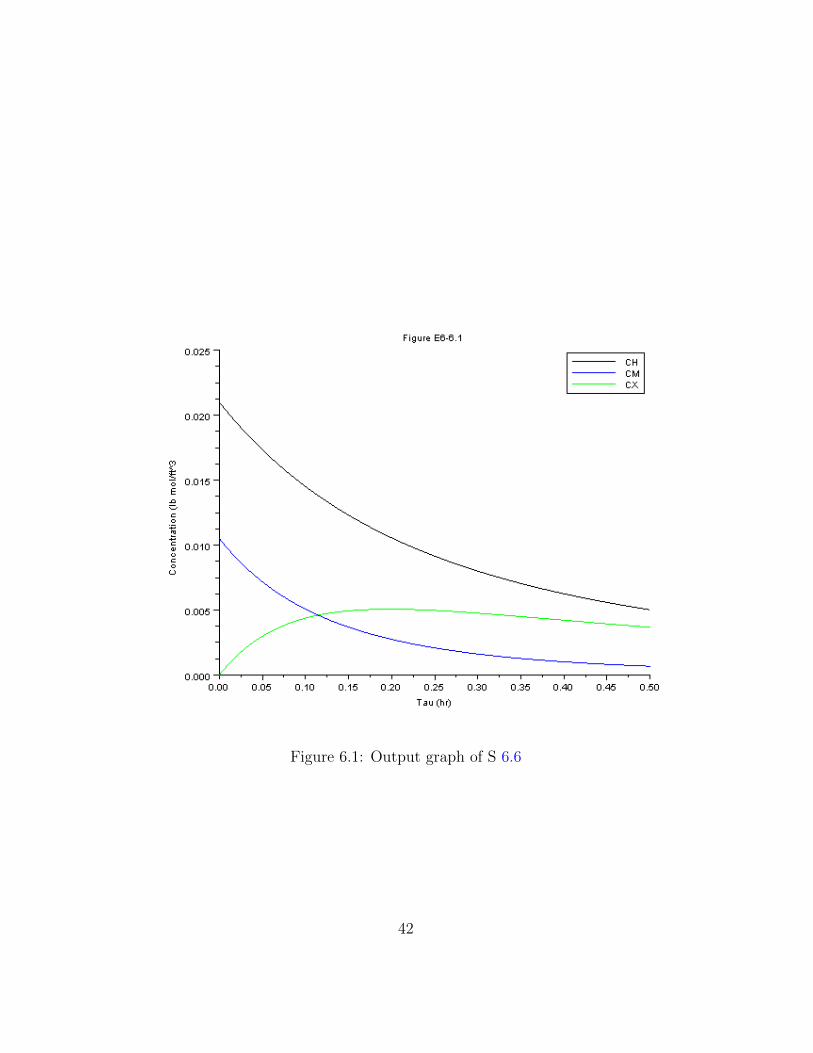
25 xtitle( ’ F i gu r e E6−6.1 ’ , ’ Tau ( hr ) ’ , ’ C o n c e n t r a t i o n( l b mol/ f t ˆ3 ’ ) ;
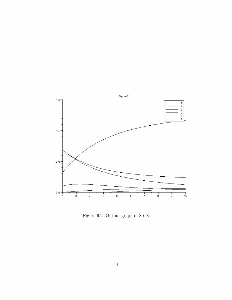
36 xtitle( ’ F igureE ’ );37 legend ([ ’B ’ ; ’A ’ ; ’C ’ ; ’D ’ ; ’E ’ ; ’F ’ ]);
43
Figure 6.2: Output graph of S 6.8
44
Chapter 7
Nonelementary ReactionKinetics
7.1 Discussion
When executing the code from the editor, use the ’Execute File into Scilab’taband not the ’Load in Scilab’tab. The .sci files of the respective problems con-tain the input parameters of the question
7.2 Scilab Code
Example 7.7 7.7data.sci
1 Curea = [.2 .02 .01 .005 .002] ’;
2 rurea = -[1.08 .55 .38 .2 .09]’;
Example 7.7 7.7.sce
1 clc
2 clear all
3 exec(” 7 . 7 data . s c i ”);4 for i=1: length(Curea)
5 x(i)= 1/Curea(i);
6 y(i) = 1/(-rurea(i));
7 end
45
Figure 7.1: Output graph of S 7.7
8 slope = (y(5)-y(1))/(x(5)-x(1));
9 plot2d(x,y)
10
11 xtitle( ’ F i gu r e E7−7.1 ’ , ’ 1/ Curea ’ , ’ 1/− r u r e a ’ ) ;
12
13 disp(” (Km/Vma = s l o p e ”)14 disp(slope)
Example 7.8 7.8data.sci
1 Km = 0.0266;
46
2 Vmax1 = 1.33;
3 Et2 = 0.001;
4 Et1 = 5;
5 X = .8;
6 Curea0 = .1;
Example 7.8 7.8.sce
1 clc
2 clear all
3 exec(” 7 . 8 data . s c i ”);4 Vmax = (Et2/Et1)*Vmax1
28 xtitle( ’ F i gu r e E7−9.1 c o n c e n t r a t i o n s as a f u n c t i o no f t ime ’ , ’ t ( hr ) ’ , ’C ( g/dmˆ3) ’ ) ;
29 legend ([ ’ Cc ’ ; ’ Cs ’ ; ’Cp ’ ]);
48
Figure 7.2: Output graph of S 7.9
49
Chapter 8
Steady State NonisothermalReactor Design
8.1 Discussion
When executing the code from the editor, use the ’Execute File into Scilab’taband not the ’Load in Scilab’tab. The .sci files of the respective problems con-tain the input parameters of the question
8.2 Scilab Code
Example 8.3 8.3data.sci
1 H0NH3 = -11020; // c a l /moleN22 H0H2 = 0;
3 HN2 = 0;
4 CpNH3 = 8.92; // c a l /moleH2 .K5 CpH2 = 6.992; // c a l /moleN2 .K6 CpN2 =6.984; // c a l /moleNH3 .K7 T = 423; //K8 TR = 298; //K
Example 8.3 8.3.sce
1 clc
50
2 clear all
3 exec(” 8 . 3 data . s c i ”);4 deltaHRx0 = 2*H0NH3 -3*H0H2 -HN2;
5 deltaCp = 2*CpNH3 -3*CpH2 -CpN2;
6 deltaHRx = deltaHRx0+deltaCp *(T-TR);
7 disp(”The heat o f r e a c t i o n on the b a s i s on the moleso f H2 r e a c t e d i s =”)
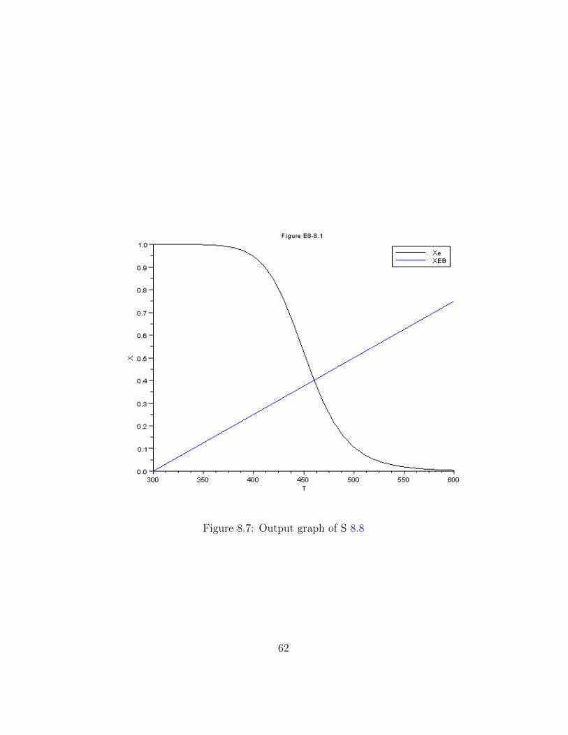
21 xtitle( ’ F i gu r e E8−12.1 ’ , ’T (K) ’ , ’G(T) ,R(T) ’ ) ;
22 legend ([ ’G(T) ’ ; ’R(T) ’ ]);
68
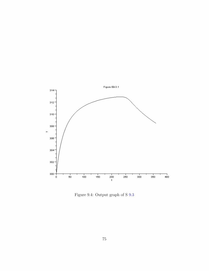
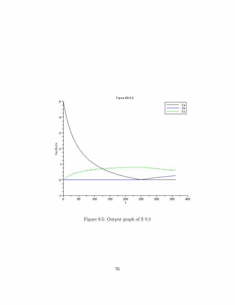
Chapter 9
Unsteady State NonisothermalReactor Design
9.1 Discussion
When executing the code from the editor, use the ’Execute File into Scilab’taband not the ’Load in Scilab’tab. The .sci files of the respective problems con-tain the input parameters of the question
9.2 Scilab Code
Example 9.1 9.1data.sci
1 t0=0;
Example 9.1 9.1.sce
1 clc
2 clear all
3 exec(” 9 . 1 data . s c i ”);4 t = 0:10:1500;
5 function w=f(t,x)
6
7 w =zeros (1,1);
69
Figure 9.1: Output graph of S 9.1
70
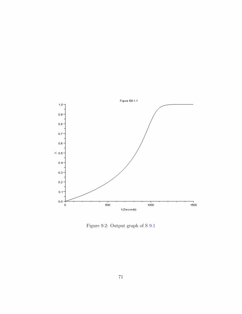
Figure 9.2: Output graph of S 9.1
71
8
9 t1 =535+90.45*x
10 k= .000273* exp (16306*((1/535) -(1/t1)));
11 w(1)=k*(1-x)
12 endfunction
13
14 X=ode([0],t0 ,t,f);
15 T=535+90.45*X;
16 scf (1)
17 plot2d(t,T);
18
19 xtitle( ’ F i gu r e E9−1.1 ’ , ’ t ( Seconds ) ’ , ’T (oR) ’ ) ;
20
21 scf (2)
22 plot2d(t,X);
23
24 xtitle( ’ F i gu r e E9−1.1 ’ , ’ t ( Seconds ) ’ , ’X ’ ) ;
Example 9.2 9.2data.sci
1 NCp =2504;
2 U=3.265+1.854;
3 Nao =9.0448;
4 UA =35.83;
5 dH= -590000;
6 Nbo =33;
7 t0=55;
Example 9.2 9.2.sce
1 clc
2 clear all
3 // t h i s code i s on ly f o r Part C4 exec(” 9 . 2 data . s c i ”);5 t = 55:1:121;
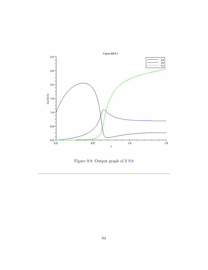
30 xtitle( ’ F i gu r e E9−8.1 ’ , ’ t ’ , ’Ca , Cb , Cc ’ ) ;
31 legend ([ ’Ca ’ ; ’Cb ’ ; ’ Cc ’ ]);32
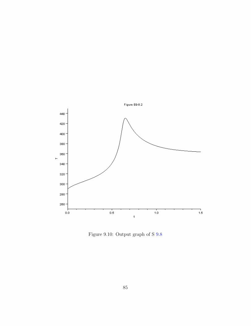
33 scf (2)
34 plot2d(t,x(4,:));
35
36 xtitle( ’ F i gu r e E9−8.2 ’ , ’ t ’ , ’T ’ ) ;
83
Figure 9.9: Output graph of S 9.8
84
Figure 9.10: Output graph of S 9.8
85
Chapter 10
Catalysis and CatalyticReactors
10.1 Discussion
When executing the code from the editor, use the ’Execute File into Scilab’taband not the ’Load in Scilab’tab. The .sci files of the respective problems con-tain the input parameters of the question
10.2 Scilab Code
Example 10.3 10.3data.sci
1 ftO =50
2 k=.0000000145*1000*60;
3 kt =1.038;
4 kb =1.39;
5 alpha =0.000098;
6 Po=40;
7 w0=0;
Example 10.3 10.3.sce
1 clc
2 clear all
86
3 exec(” 1 0 . 3 data . s c i ”);4 w = 0:10:10000;
5
6 function W=f(w,x)
7
8 W =zeros (1,1);
9
10 pt0 =.3*Po;
11 y=(1- alpha*w)^.5;
12 ph=pt0*(1.5-x)*y;
13 pt=pt0*(1-x)*y;
14 pb=2*pt0*x*y;
15 rt=-k*kt*ph*pt/(1+kb*pb+kt*pt);
16 rate=-rt;
17 W(1)=-rt/ftO;
18 endfunction
19 pt0 =.3*Po;
20 X=ode([0],w0 ,w,f);
21
22
23 for i =1: length(X)
24 y(1,i)=(1-alpha*w(1,i))^.5;
25 ph(1,i)=pt0 *(1.5 -X(1,i))*y(1,i);
26 pt(1,i)=pt0*(1-X(1,i))*y(1,i);
27 pb(1,i)=2* pt0*X(1,i)*y(1,i)
28 end
29
30 m1 = X’;
31 m2=y’;
32 scf (1)
33 plot2d(w’,[m1 m2]);
34
35 xtitle( ’ F i gu r e E10−3.1 ’ , ’w ’ , ’ x , y ’ ) ;
36 legend ([ ’ x ’ ; ’ y ’ ]);37
38 scf (2)
39 l1=ph’
40 l2=pt’
87
Figure 10.1: Output graph of S 10.5
41 l3=pb’
42 plot2d(w’,[l1 l2 l3]);
43
44 xtitle( ’ F i gu r e E10−3.2 ’ , ’w ’ , ’ ph , pt , pb ’ ) ;
When executing the code from the editor, use the ’Execute File into Scilab’taband not the ’Load in Scilab’tab. The .sci files of the respective problems con-tain the input parameters of the question
11.2 Scilab Code
Example 11.1 11.1data.sci
1 DAB =1e-6;
2 CT0 =.1; // kmol /mˆ33 yAb =.9;
4 yAs =.2;
5 s=1e-6;
6 c=.1;
Example 11.1 11.1.sce
1 clc
2 clear all
3 exec(” 1 1 . 1 data . s c i ”);
94
4 WAZ1=DAB*CT0*(yAb -yAs)/s;
5 WAZ2=c*DAB*CT0*log((1-yAs)/(1-yAb))/s;
6 disp(WAZ1)
7 disp(WAZ2)
Example 11.3 11.3data.sci
1 D=.0025; //m2 L=.005; //m3 phi =.3;
4 U=15; //m/ s ;5 v=4.5e-4; //mˆ2/ s6 r=.0025/2;
7 Lp =.005;
8 DAB0 =.69e-4;
9 T=750;
10 T0=298;
11 z=.05; //m
Example 11.3 11.3.sce
1 clc
2 clear all
3 exec(” 1 1 . 3 data . s c i ”);4 // t h i s i s on ly Part A o f the problem .5 dp=(6*(D^2)*L/4) ^(1/3);
6 disp(” P a r t i c l e d i amete r dp =”)7 disp(dp)
8 disp(”m”)9 ac=6*(1- phi)*(1/dp);
10 disp(” S u r f a c e a r ea pervo lume o f bed =”)11 disp(ac)
12 disp(”mˆ2/mˆ3 ”)13 Re =dp*U/v;
14 Y=(2*r*Lp+2*r^2)/dp^2;
15 Reprime=Re/((1-phi)*Y);
16 DAB=DAB0*(T/T0)^(1.75);
17 Sc=v/DAB;
95
18 Shprime =(( Reprime)^.5)*Sc ^(1/3);
19 kc=DAB*(1-phi)*Y*( Shprime)/(dp*phi);
20 X=1-exp(-kc*ac*z/U);
21 disp(”X =”)22 disp(X)
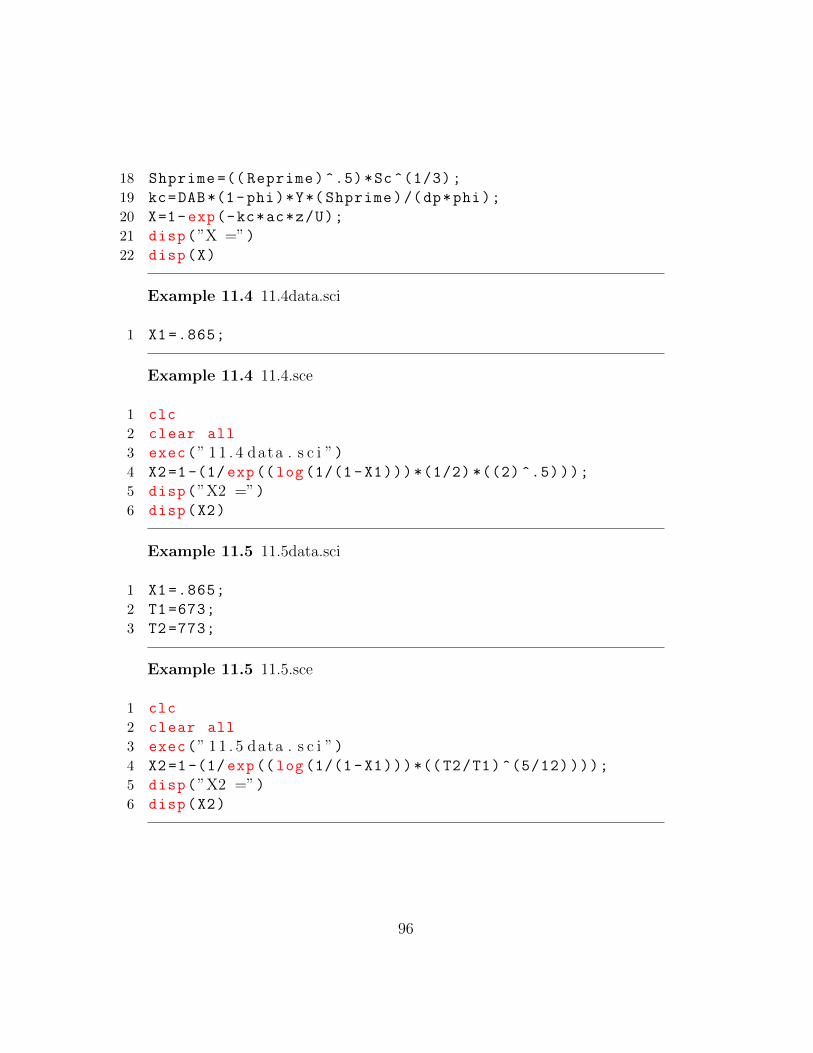
Example 11.4 11.4data.sci
1 X1 =.865;
Example 11.4 11.4.sce
1 clc
2 clear all
3 exec(” 1 1 . 4 data . s c i ”)4 X2=1-(1/ exp((log(1/(1-X1)))*(1/2) *((2) ^.5)));
5 disp(”X2 =”)6 disp(X2)
Example 11.5 11.5data.sci
1 X1 =.865;
2 T1=673;
3 T2=773;
Example 11.5 11.5.sce
1 clc
2 clear all
3 exec(” 1 1 . 5 data . s c i ”)4 X2=1-(1/ exp((log(1/(1-X1)))*((T2/T1)^(5/12))));
5 disp(”X2 =”)6 disp(X2)
96
Chapter 12
Diffusion and Reaction inPours Catalysts
12.1 Discussion
When executing the code from the editor, use the ’Execute File into Scilab’taband not the ’Load in Scilab’tab. The .sci files of the respective problems con-tain the input parameters of the question
12.2 Scilab Code
97
Chapter 13
Distributions of ResidenceTimes for Chemical Reactions
13.1 Discussion
When executing the code from the editor, use the ’Execute File into Scilab’taband not the ’Load in Scilab’tab. The .sci files of the respective problems con-tain the input parameters of the question
When executing the code from the editor, use the ’Execute File into Scilab’taband not the ’Load in Scilab’tab. The .sci files of the respective problems con-tain the input parameters of the question