Scilab Code for Unit Operations of Chemical Engineering by Warren L. McCabe, Julian C. Smith, Peter Harriott 1 Created by Prashant Dave Sr. Research Fellow Chem. Engg. Indian Institute of Technology, Bombay College Teacher and Reviewer ............. .............. IIT Bombay 30 October 2010 1 Funded by a grant from the National Mission on Education through ICT, http://spoken-tutorial.org/NMEICT-Intro. This text book companion and Scilab codes written in it can be downloaded from the ”Textbook Companion Project” Section at the website http://scilab.in/
Transcript
Scilab Code forUnit Operations of Chemical Engineering
by Warren L. McCabe, Julian C. Smith, PeterHarriott1
Created byPrashant Dave
Sr. Research FellowChem. Engg.
Indian Institute of Technology, Bombay
College Teacher and Reviewer...........................
IIT Bombay
30 October 2010
1Funded by a grant from the National Mission on Education through ICT,http://spoken-tutorial.org/NMEICT-Intro. This text book companion and Scilabcodes written in it can be downloaded from the ”Textbook Companion Project”Section at the website http://scilab.in/
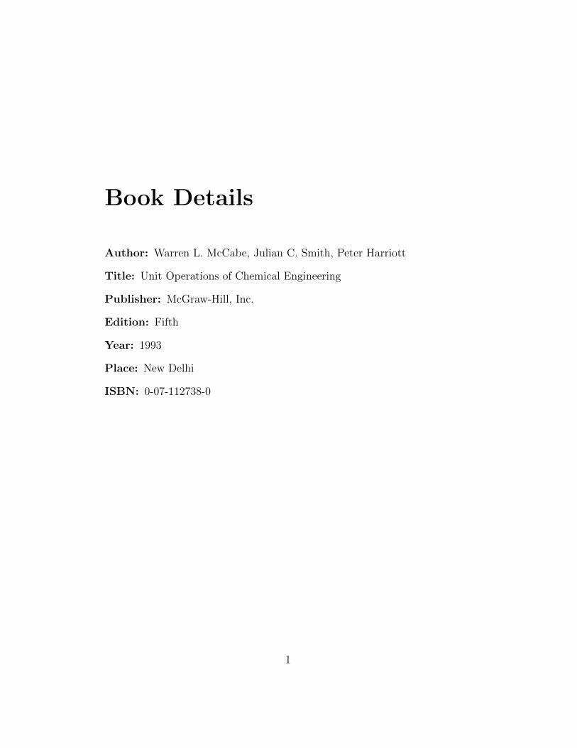
Book Details
Author: Warren L. McCabe, Julian C. Smith, Peter Harriott
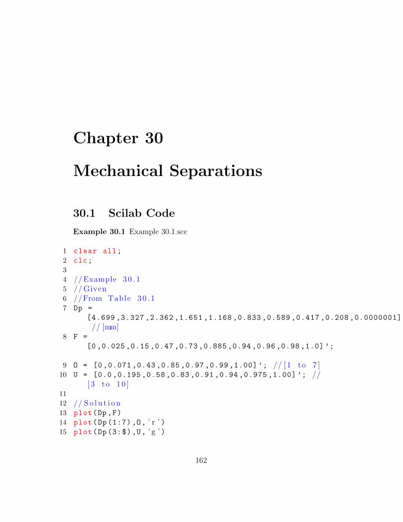
6 // S o l u t i o n7 // ( a )8 // Using Eq . ( 1 . 6 , ) , ( 1 . 2 6 ) , and ( 1 . 2 7 )9 // Let N = 1N10 N = 0.3048/(9.80665*0.45359237*0.3048); // [ l b f ]11
12 // ( b )13 // Using ( 1 . 3 8 ) , ( 1 . 1 6 ) , ( 1 . 2 6 ) , and ( 1 . 3 1 )14 // Let B = 1 Btu15 B = 0.45359237*1000/1.8; // [ c a l ]16
15 disp( ’mm’ ,Rm , ’ The r e a d i n g i n the mamometer i s (Rm) =’ )
Example 2.2 Example 2.2.sce
11
1 clear all;
2 clc;
3
4 // Example 2 . 25
6 // ( a )7 // Using Eq . ( 2 . 1 5 )8 t = (100*1.1) /(1153 -865)
9 rate_each_stream = (1500*42) /(24*60)
10 total_liquid_holdup = 2*43.8*23
11 vol = total_liquid_holdup /0.95
12 disp( ’ g a l ’ ,vol , ’ v e s s e l s i z e = ’ )13
14 // ( b ) tank d iamete r15 Zt = 0.90*4
16 ZA1 = 1.8 // [ f t ] ;17 ZA2 = 1.8 + (3.6 -1.8) *(54/72)
18 disp( ’ f t ’ ,ZA2 , ’ tank d iamete r = ’ )
12
Chapter 4
Basic Equations of Fluid Flow
4.1 Scilab Code
Example 4.1 Example 4.1.sce
1 clear all;
2 clc;
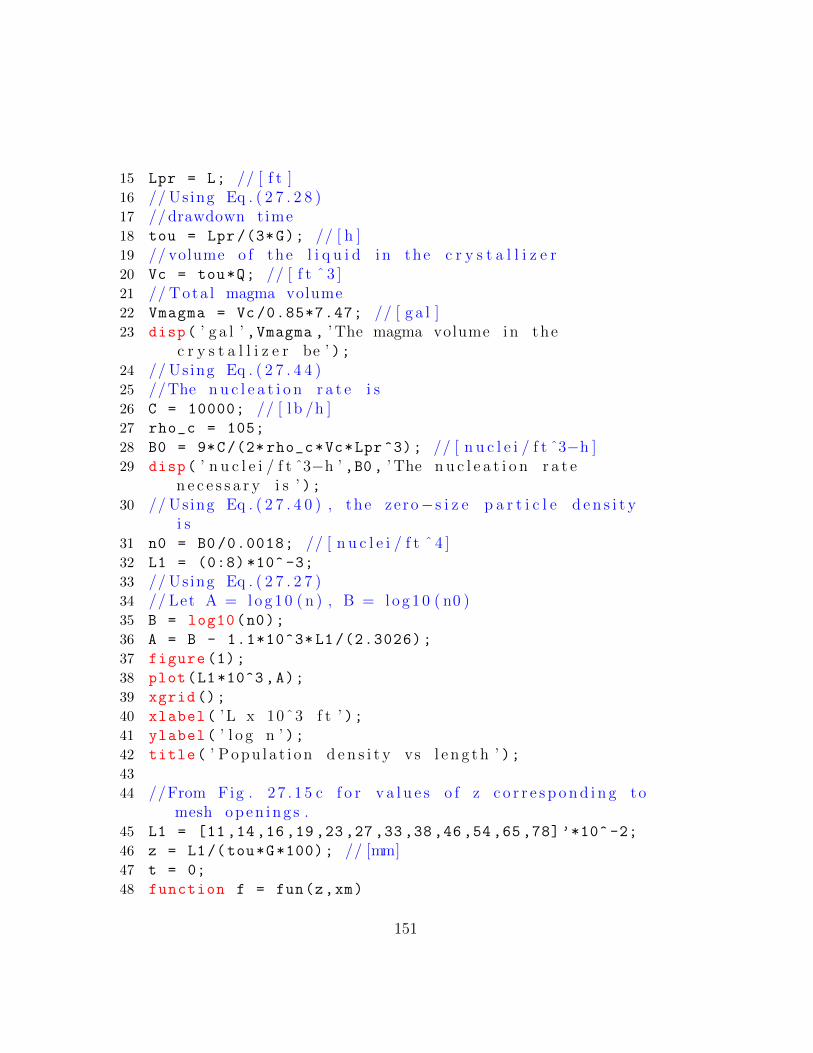
3
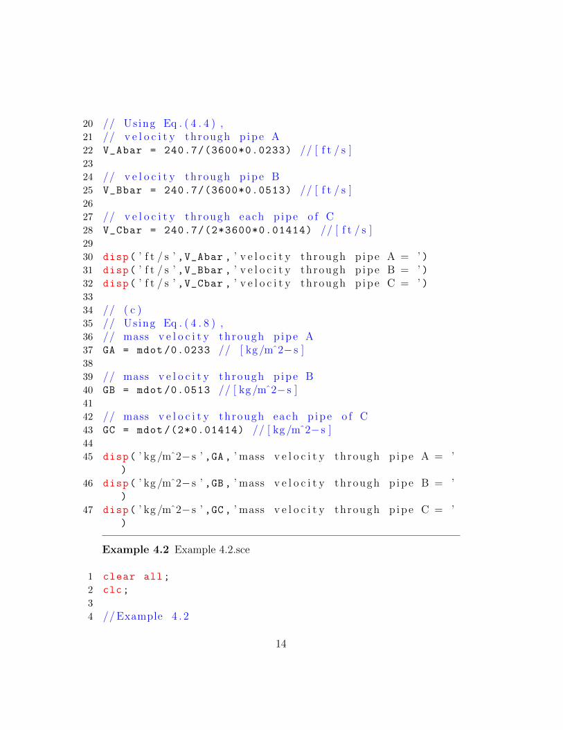
4 // Example 4 . 15
6 // ( a )7 // d e n s i t y o f the f l u i d8 rho = 0.887*62.37; // [ l b / f t ˆ 3 ]9 // t o t a l v o l u m e t r i c f l o w r a t e10 q = 30*60/7.48; // [ f t ˆ3/ hr ]11 // mass f l o w r a t e i n p ip e A and p ipe B i s same12 mdot = rho*q // [ l b / hr ]13 // mass f l o w r a t e i n each p ipe o f C i s h a l f o f the
t o t a l f l o w14 mdot_C = mdot/2 // [ l b / hr ]15 disp( ’ l b / hr ’ ,mdot , ’ mass f l o w r a t e p ip e A = ’ )16 disp( ’ l b / hr ’ ,mdot , ’ mass f l o w r a t e p ip e B = ’ )17 disp( ’ l b / hr ’ ,mdot_C , ’ mass f l o w r a t e p ip e C = ’ )18
19 // ( b )
13
20 // Using Eq . ( 4 . 4 ) ,21 // v e l o c i t y through p ipe A22 V_Abar = 240.7/(3600*0.0233) // [ f t / s ]23
24 // v e l o c i t y through p ipe B25 V_Bbar = 240.7/(3600*0.0513) // [ f t / s ]26
27 // v e l o c i t y through each p ipe o f C28 V_Cbar = 240.7/(2*3600*0.01414) // [ f t / s ]29
30 disp( ’ f t / s ’ ,V_Abar , ’ v e l o c i t y through p ipe A = ’ )31 disp( ’ f t / s ’ ,V_Bbar , ’ v e l o c i t y through p ipe B = ’ )32 disp( ’ f t / s ’ ,V_Cbar , ’ v e l o c i t y through p ipe C = ’ )33
34 // ( c )35 // Using Eq . ( 4 . 8 ) ,36 // mass v e l o c i t y through p ipe A37 GA = mdot /0.0233 // [ kg /mˆ2− s ]38
39 // mass v e l o c i t y through p ipe B40 GB = mdot /0.0513 // [ kg /mˆ2− s ]41
42 // mass v e l o c i t y through each p ipe o f C43 GC = mdot /(2*0.01414) // [ kg /mˆ2− s ]44
45 disp( ’ kg /mˆ2− s ’ ,GA , ’ mass v e l o c i t y through p ipe A = ’)
46 disp( ’ kg /mˆ2− s ’ ,GB , ’ mass v e l o c i t y through p ipe B = ’)
47 disp( ’ kg /mˆ2− s ’ ,GC , ’ mass v e l o c i t y through p ipe C = ’)
Example 4.2 Example 4.2.sce
1 clear all;
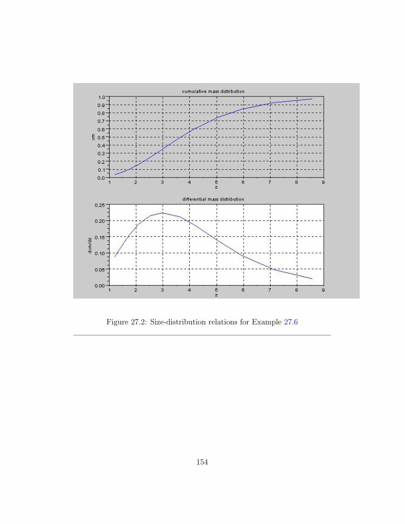
2 clc;
3
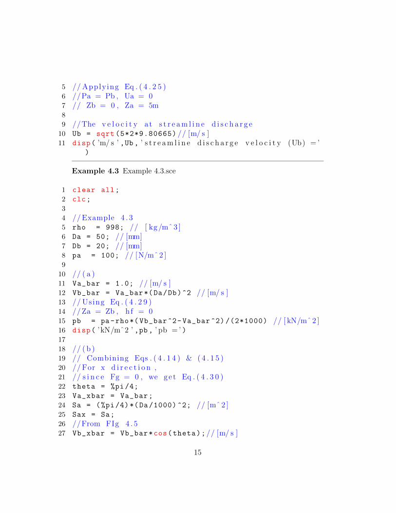
4 // Example 4 . 2
14
5 // Apply ing Eq . ( 4 . 2 5 )6 //Pa = Pb , Ua = 07 // Zb = 0 , Za = 5m8
9 //The v e l o c i t y at s t r e a m l i n e d i s c h a r g e10 Ub = sqrt (5*2*9.80665) // [m/ s ]11 disp( ’m/ s ’ ,Ub , ’ s t r e a m l i n e d i s c h a r g e v e l o c i t y (Ub) = ’
)
Example 4.3 Example 4.3.sce
1 clear all;
2 clc;
3
4 // Example 4 . 35 rho = 998; // [ kg /mˆ 3 ]6 Da = 50; // [mm]7 Db = 20; // [mm]8 pa = 100; // [N/mˆ 2 ]9
10 // ( a )11 Va_bar = 1.0; // [m/ s ]12 Vb_bar = Va_bar *(Da/Db)^2 // [m/ s ]13 // Using Eq . ( 4 . 2 9 )14 //Za = Zb , h f = 015 pb = pa -rho*( Vb_bar^2-Va_bar ^2) /(2*1000) // [ kN/mˆ 2 ]16 disp( ’kN/mˆ2 ’ ,pb , ’ pb = ’ )17
18 // ( b )19 // Combining Eqs . ( 4 . 1 4 ) & ( 4 . 1 5 )20 // For x d i r e c t i o n ,21 // s i n c e Fg = 0 , we g e t Eq . ( 4 . 3 0 )22 theta = %pi /4;
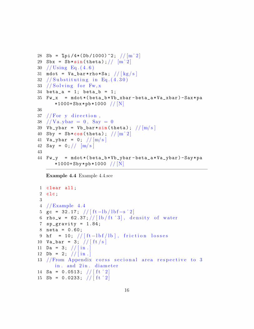
28 Sb = %pi /4*(Db /1000) ^2; // [mˆ 2 ]29 Sbx = Sb*sin(theta);// [mˆ 2 ]30 // Using Eq . ( 4 . 6 )31 mdot = Va_bar*rho*Sa; // [ kg / s ]32 // S u b s t i t u t i n g i n Eq . ( 4 . 3 0 )33 // S o l v i n g f o r Fw, x34 beta_a = 1; beta_b = 1;
37 // For y d i r e c t i o n ,38 // Va ybar = 0 , Say = 039 Vb_ybar = Vb_bar*sin(theta); // [m/ s ]40 Sby = Sb*cos(theta); // [mˆ 2 ]41 Va_ybar = 0; // [m/ s ]42 Say = 0; // [m/ s ]43
4 // Example 4 . 45 gc = 32.17; // [ f t −l b / l b f −s ˆ 2 ]6 rho_w = 62.37; // [ l b / f t ˆ 3 ] , d e n s i t y o f water7 sp_gravity = 1.84;
8 neta = 0.60;
9 hf = 10; // [ f t − l b f / l b ] , f r i c t i o n l o s s e s10 Va_bar = 3; // [ f t / s ]11 Da = 3; // [ i n . ]12 Db = 2; // [ i n . ]13 //From Appendix c o r s s s e c i o n a l a r ea r e s p e c t i v e to 3
i n . and 2 i n . d i amete r14 Sa = 0.0513; // [ f t ˆ 2 ]15 Sb = 0.0233; // [ f t ˆ 2 ]
16
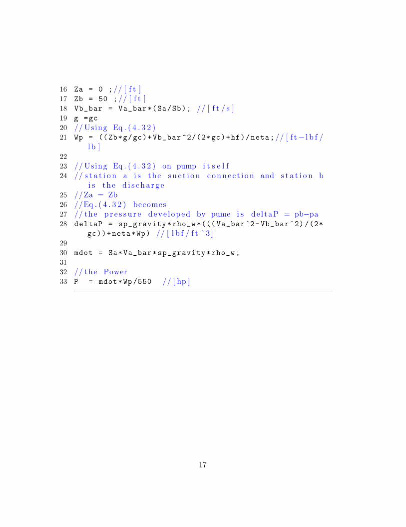
16 Za = 0 ;// [ f t ]17 Zb = 50 ;// [ f t ]18 Vb_bar = Va_bar *(Sa/Sb); // [ f t / s ]19 g =gc
20 // Using Eq . ( 4 . 3 2 )21 Wp = ((Zb*g/gc)+Vb_bar ^2/(2* gc)+hf)/neta;// [ f t − l b f /
l b ]22
23 // Using Eq . ( 4 . 3 2 ) on pump i t s e l f24 // s t a t i o n a i s the s u c t i o n c o n n e c t i o n and s t a t i o n b
i s the d i s c h a r g e25 //Za = Zb26 //Eq . ( 4 . 3 2 ) becomes27 // the p r e s s u r e deve l oped by pume i s de l t aP = pb−pa28 deltaP = sp_gravity*rho_w *((( Va_bar^2-Vb_bar ^2) /(2*
gc))+neta*Wp) // [ l b f / f t ˆ 3 ]29
30 mdot = Sa*Va_bar*sp_gravity*rho_w;
31
32 // the Power33 P = mdot*Wp/550 // [ hp ]
17
Chapter 5
Flow of Incompressible Fluidsin Conduits and Thin Layers
5.1 Scilab Code
Example 5.1 Example 5.1.sce
1 clear all;
2 clc;
3
4 // Example 5 . 15 // Given6 mu = 0.004; // [ kg /m−s ]7 D = 0.0779; // [m]8 rho = 0.93*998; // [ kg /mˆ 3 ]9 L = 45; // [m]
10
11 // For f i t t i n g s , form Table 5 . 112 sum_Kf = 0.9 + 2*0.2;
13 //From Eq . ( 4 . 2 9 ) , assuming a l p h a a = 1 ,14 // s i n c e pa = pb , and Va bar = 015 //A = Vb bar ˆ2/2 + hf = g ∗ ( Za−Zb )16 A = 9.80665*(6+9); // [mˆ2/ s ˆ 2 ]17 // Using Fig 5 . 918 f = 0.0055;
18
19 // Using Eq . ( 5 . 6 8 ) , There i s no exapns i on l o s s and Ke= 0 .
20 //From Eq . ( 5 . 6 6 ) , s i n c e Sa i s ve ry l age , Kc = 0 . 4 .Hence
21 Vb_bar = sqrt (294.2/(2.7+2311*f));// [m/ s ]22 //From Appendix 5 , c r o s s s e c t i o n a l a r ea o f the p ip e23 S = 0.00477; // [mˆ 2 ]24 flow_rate = S*Vb_bar *3600 // [mˆ3/ hr ]
10 gc = 1; // [ f t −l b / l b f −s ˆ 2 ]11 //At Entrance12 p0 = 20; // [ atm ]13 T0 = 555.6; // [K]14
15 // ( a )16 // Using Eq . ( 6 . 2 8 )17 // P r e s s u r e at t h r o a t18 pt = (1/(1+(( gama -1)/2)*Nma ^2) ^(1/(1 -1/ gama)))*p0
// [ atm ]19 //From Eq . ( 6 . 1 0 )
20
20 rho0 = (p0*M)/(R*T0); // [ kg /mˆ 3 ]21 // Using Eq . ( 6 . 1 0 ) and Eq . ( 6 . 2 6 ) , the v e l o c i t y i n
the t h r o a t22 ut = sqrt ((2* gama*gc*R*T0)/(M*(gama -1))*(1-(pt/p0)
^(1 -1/ gama))); // [mˆ3−am/ kg ] ˆ 0 . 523 // In terms o f [m/ s ] , Us ing Appendix 2 , 1 atm =
1 .01325∗10ˆ [N/mˆ 2 ]24 ut = ut*sqrt (1.01325*10^5) // [m/ s ]25 // Using Eq . ( 6 . 2 3 ) , d e n s i t y at t h r o a t26 rho_t = rho0*(pt/p0)^(1/ gama) // [ kg /mˆ 3 ]27 //The mass v e l o c i t y at the th roa t ,28 Gt = ut*rho_t // [ kg /mˆ2− s ]29 // Using Eq . ( 6 . 2 4 ) , The t empera tu r e at t h r o a t30 Tt = T0*(pt/p0)^(1-1/ gama) // [K]31
/(2.4)) // [ l b / f t ˆ 3 ]34 // Using Eq . ( 6 . 3 9 )35 pstar = p0*Ma_a/sqrt (1.2) // [ atm ]36 // Mass v e l o c i t y through the e n t i r e p ip e37 G = 0.795* ua // [ l b / f t ˆ2− s ]38 ustar = G/rho_star // [ f t / s ]39
40 // ( c )41 // Using Eq . ( 6 . 4 5 ) with f Lmax rh = 40042
43 err = 1;
44 eps = 10^-3;
45 Ma_ac = rand (1,1);
46 i =1;
47 while((err >eps))
48 A = 2*(1+(( gama -1)/2)*Ma_ac ^2)/(( gama +1)*Ma_ac ^2);
49 B = gama *400+1+( gama +1)*log(A)/2;
50 Ma_anew = sqrt (1/B);
51 err = Ma_ac -Ma_anew;
52 Ma_ac = Ma_anew;
53 end
54 Ma_ac;
55 uac = Ma_ac*ua/Ma_a // [ f t / s ]56 Gc = uac *0.795 // [ l b / f t ˆ2− s ]
Example 6.3 Example 6.3.sce
1 clear all;
23
2 clc;
3
4 // Example 6 . 35 // Given6 pa = 2.7; // [ atm ]7 T = 288; // [K]8 D = 0.075; // [m]9 L = 70; // [m]
10 Vbar = 60; // [m/ s ]11 M = 29;
12 rh = D/4; // [m]13 mu = 1.74*10^ -5 // [ kg /m−s ] Appendix 814 rho_a = (29/22.4) *(2.7/1) *(273/288) // [ kg /mˆ 3 ]15 R = 82.056*10^ -3;
16 G = Vbar*rho_a // [ kg /mˆ2− s ]17 Nre = D*G/mu;
28 // ( b )29 // Using ’ ac ’ i n p l a c e o f ’ g ’ i n Eq . ( 7 . 4 5 )30 K = K*50^(1/3); // S i n c e on ly a c c e l e r a t i o n changes31 // Et imat ing32 N_rep = 80; //From Fig . ( 7 . 6 )33 Cd = 1.2;
4 // Example 7 . 25 // Given6 g = 32.174; // [ f t −l b / l b f −s ˆ 2 ]7 eps = 0.8;
8 speg_s = 4.0;
9 speg_c = 1.594;
10 Ds = 0.004; // [ i n . ]11 rho_w = 62.37; // [ l b f / f t ˆ 3 ]12 delta_speg = speg_s -speg_c;
13 delta_rho = rho_w*delta_speg; // [ l b f / f t ˆ 3 ]
26
14 rho_c = rho_w*speg_c; // [ l b f / f t ˆ 3 ]15 //From Appendix 916 mu = 1.03; // [ cP ]17 // Using Eq . ( 7 . 4 5 )18 K = Ds/12*(g*rho_c *( delta_rho)/(mu *6.72*10^ -4) ^2)
^(1/3);
19 // Using Eq . ( 7 . 4 0 )20 ut = g*(Ds/12) ^2* delta_rho /(18*mu *6.72*10^ -4) // [ f t /
s ]21
22 //The t e r m i n a l v e l o c i t y i n h i n d e r e d s e t t l i n g23 // C a l c u l a t i n g Reynolds Number24 Nre = ut*rho_c*Ds/(12* mu *6.72*10^ -4);
25 //From Fig . ( 7 . 7 )26 n = 4.1;
27 // Using Eq . ( 7 . 4 6 )28 us = ut*eps^n // [ f t / s ]
Example 7.3 Example 7.3.sce
1 clear all;
2 clc;
3
4 // Example 7 . 35 //The q u a n t i t i e s needed a r e6 mu = 0.01; // [ P ]7 delta_rho = 0.24; // [ g/cm ˆ 3 ]8 // Using Eq . ( 7 . 5 1 ) , s o l v i n g the q u a d r a t i c e q u a t i o n f o r
Vom bar9 a = 1.75*1/(0.11*0.4^3);
10 b = 150*0.01*0.6/(0.11^2*0.4^3);
11 c = - 980*0.24;
12 Vom_bar = (-b+sqrt(b^2-4*a*c))/(2*a); // [ cm/ s ]13 // Cor r e spond ing Reynolds number14 Nre = 0.11*0.194*0.124/0.01;
4 // Example 8 . 15 // Given6 vdot = 40; // [ g a l /min ]7 pb = 50; // [ l b f / i n . ˆ 2 ]8 Za = 4; // [ f t ]9 Zb = 10; // [ f t ]
10 hfs = 0.5; // [ l b f / i n . ˆ 2 ]11 hfd = 5.5; // [ l b f / i n . ˆ 2 ]12 neta = 0.6;
13 rho = 54; // [ l b / f t ˆ 3 ]14 pv = 3.8; // [ l b f / i n . ˆ 2 ]15 g = 9.8; // [m/ s ˆ 2 ]16 gc = 32.17 // [ f t −l b / l b f −s ˆ 2 ]17 hf = hfs+hfd; // [ l b f / i n . ˆ 2 ]18 // ( a )
29
19 // Using data from Appendix 520 Vb_bar = vdot /6.34; // [ f t / s ]21 // Using Eq . ( 4 . 3 2 )22
^2/(2* gc))+(hf *144/54) -(14.7*144/54); // [ f t − l b f /l b ]
24 delta_H = Wp_neta;
25
26 // ( b )27 mdot = vdot*rho /(7.48*60); // [ l b / s ]28 // Using Eq . ( 8 . 7 ) , the input power i s29 Pb = mdot*delta_H /(550* neta) // [ hp ]30
31 // ( c )32 padash = 14.7*144/ rho;
33 //The vapor p r e s s u r e c o r r e s p o n d i n g to a head34 hv = pv *144/ rho; // [ f t − l b f / l b ]35 // f r i c t i o n i n the s u c t i o n l i n e36 hfs = 0.5*144/ rho ; // [ f t − l b f / l b ]37 // Using Eq . ( 8 . 7 ) , v a l u e o f a v a i l a b l e38 NPSH = padash -hv -hfs -Za // [ f t ]
Example 8.2 Example 8.2.sce
1 clear all;
2 clc;
3
4 // Example 8 25 // Given6 pa = 29; // [ i n . Hg ]7 pb = 30.1; // [ i n . Hg ]8 va = 0; // [ f t / s ]9 vb = 150; // [ f t / s ]10 Ta = 200; // [ F ]11 vdot = 10000; // [ f t ˆ3/ min ]12 neta = 0.65;
13 M = 31.3;
30
14 R = 29.92;
15 gc = 32.17; // [ f t −l b / l b f −s ˆ 2 ]16 // a c t u a l s u c t i o n d e n s i t y17 rho_a = M*pa *(460+60) /(378.7*30*(460+ Ta)); // [ l b / f t
ˆ 3 ]18 // a c u a l d i s c h a r g e d e n s i t y19 rho_b = rho_a*pb/pa; // [ l b / f t ˆ 3 ]20 // ave rage d e n s i t y o f the f l o w i n g gas21 rho = (rho_a+rho_b)/2; // [ l b / f t ˆ 3 ]22 // mass f l o w r a t e23 mdot = vdot*M/(378.7*60) // [ l b / s ]24 // deve l oped p r e s s u r e25 dev_p = (pb -pa)*144*14.7/(R*rho); // [ f t − l b f / l b ]26 // v e l o c i t y head27 vel_head = vb ^2/(2* gc); // [ f t − l b f / l b ]28 // Using Eq . ( 8 . 1 ) , a l p h a a = a lpha b = 1 , va = 0 , Za =
Zb ,29 Wp = (dev_p+vel_head)/neta // [ f t − l b f / l b ]30 // Using Eq . ( 8 . 4 )31 Pb = mdot*Wp/550 // [ hp ]
Example 8.3 Example 8.3.sce
1 clear all;
2 clc;
3
4 // Example 8 . 35 // Given6 vdot = 180; // [ f t ˆ3/ min ]7 pa = 14; // [ l b f / i n . ˆ 2 ]8 pb = 900; // [ l b f / i n . ˆ 2 ]9 Ta = 80+460; // [K]10 q0 = 0.063; // [mˆ3/ s ]11 Cp = 9.3; // [ Btu/ lbmol−F ]12 gama = 1.31;
13 delta_Tw = 20; // [ F ]14 // ( a )15 neta = 0.80;
31
16 // For a m u l t i s t a g e compre s so r the t o t a l power i s aminimum i f each s t a g e doed the same amount o fwork
17 // Hence u s i n g same c o p r e s s i o n r a t i o n f o r each s t a g e18 // Using Eq . ( 8 . 2 5 )19 // For one s t a g e20 comp_ratio = (900/14) ^(1/3);
21 // Using Eq . ( 8 . 2 9 ) , the power r e q u i r e d by each s t a g e22 Pb = (Ta*q0*gama*vdot)*( comp_ratio ^(1-1/ gama) -1)
/(520*( gama -1)*neta); // [ hp ]23 // Tota l Power24 Pt = 3*Pb // [ hp ]25
26 // ( b )27 // Using Eq . ( 8 . 2 2 ) , the t empera tu r e at the e x i t o f
each s t a g e28 Tb = Ta*comp_ratio ^(1 -1/ gama) // [R]29
30 // ( c ) S i n c e 1 l b mol = 3 7 8 . 7 s td f t ˆ3 , the f l o w r a t ei s
31 vdot = vdot *60/378.7; // [ l b mol/h ]32 // Heat l oad i n each c o o l e r i s33 Hl = vdot*Cp*(Tb -Ta) // [ Btu/h ]34 // Tota l heat l o s s35 Htotal = 3*Hl; // [ Btu/h ]36 // Coo l i ng water r e q u i r e m e n t37 cwr = Htotal/delta_Tw // [ l b /h ]
Example 8.4 Example 8.4.sce
1 clear all;
2 clc;
3
4 // Example 8 . 45 // Given6 q = 75/3600 ; // [mˆ3/ s ]7 rho = 62.37*16.018; // [ kg /mˆ 3 ] From Appendix 48 Cv = 0.98;
32
9 g = 9.80665; // [m/ s ˆ 2 ]10 Sw = 1;
11 Sm = 13.6;
12 h = 1.25; // [m]13 // ( a )14 // Using Eq . ( 2 . 1 0 )15 delta_p = g*h*(Sm-Sw)*rho ; // [N/mˆ 2 ]16 // Using Eq . ( 8 . 3 6 ) , n e g l e c t i n g the e f f e c t o f be ta17 Sb = q/(Cv*sqrt (2* delta_p/rho));
18 Db = sqrt (4*Sb/%pi)*100 // [mm]19
20 // ( b )21 press_loss = 0.1* delta_p; // [N/mˆ 2 ]22 // Power r e q u i r e d at f u l l f l o w23 P = q*press_loss /1000 // [kW]
Example 8.5 Example 8.5.sce
1 clear all;
2 clc;
3
4 // Example 8 . 55 // Given6 T = 100; // [ F ]7 mu_O = 5.45; // [ cP ]8 spg_O = 0.8927;
9 spg_m = 13.6;
10 spg_gl = 1.11;
11 q = 12000; // [ bb l /d ]12 rho_ratio = 0.984;
13 rho_w = 62.37; // [ l b / f t ˆ 3 ]14 h = 30; // [ i n . ]15 gc = 32.174; // [ f t −l b / l b f −s ˆ 2 ]16 // ( a )17 // Using Eq . ( 8 . 4 2 )18 rhoB_60 = spg_O*rho_w; // [ l b / f t ˆ 3 ]19 rho_100 = spg_O*rho_w*rho_ratio; // [ l b / f t ˆ 3 ]20 mdot = q*42* rhoB_60 /(24*3600*7.48); // [ l b / s ]
33
21 Da = 4.026/12; // [ f t ]22 delta_p = h/12*( spg_m -spg_gl)*rho_w *(1); // [ l b f / f t
25 Do = Da*beeta; // [ f t ]26 // the o r i f i c e d i amete r27 D = 12*Do // [ i n . ]28
29 // ( b )30 // Using Fig . 8 . 2 0 , the f r a c t i o n o f d i f f e r e n t i a l
p r e s s u r e l o s s i s31 fra_prss_loss = 0.68;
32 //Maximum power consumption33 P = mdot*delta_p*fra_prss_loss /( rho_ratio*rho_w*
spg_O *550) // [ hp ]
Example 8.6 Example 8.6.sce
1 clear all;
2 clc;
3
4 // Example 8 . 45 // Given6 Cpt = 0.98;
7 Ta = 200; // [ F ]8 Da = 36; // [ i n . ]9 pa = 15.25; // [ i n . ]
10 h = 0.54; // [ i n . ]11 P = 29.92; // [ i n . ]12 spg_m =13.6; // [ s p e c i f i c g r a v i t y o f mercury ]13 rho_w = 62.37; // [ l b / f t ˆ 3 ]14 gc = 32.174; // [ f t −l b / l b f −s ˆ 2 ]15 // Using Eq . ( 8 . 5 2 )16 Pabs = P+pa/spg_m; // [ i n . ]17 rho = 29*492*31.04/(359*(200+460) *29.92); // [ l b / f t
ˆ 3 ]
34
18 //From manometer r e a d i n g19 delta_p = h/12* rho_w // [ l b f / f t ˆ 3 ]20
21 // Using Eq . ( 8 . 5 3 , m∗aximum v e l o c i t y , assuming Nma i sn e g l i g i b l e
22 umax = Cpt*sqrt (2*gc*delta_p/rho) // [ f t / s ]23 //The r e y n o l d s number based on maximum v e l o c i t y24 mu_air = 0.022 ; // [ cP ] form Appendix 825 Nre_max = (Da/12)*umax*rho/( mu_air *0.000672);
26 // Using Fig 5 . 7 , to o b t a i n ave rage v e l o c i t y27 Vbar = 0.86* umax // [ f t / s ]28 Nre = Nre_max *0.86;
29 //The v o l u m e t r i c f l o w r a t e30 q = Vbar*(Da/12) ^2*%pi /4*520/660* Pabs/P*60 // [ f t ˆ3/
min ]
35
Chapter 9
Agitation and Mixing ofLiquids
9.1 Scilab Code
Example 9.1 Example 9.1.sce
1 clear all;
2 clc;
3
4 // Exapmle 9 . 15 // Given6 Dt = 6; // [ f t ]7 h = 2; // [ f t ]8 n = 90/60; // [ rp s ]9 mu = 12*6.72*10^ -4; // [ l b / f t −s ]
10 g = 32.17; // [ f t / s ˆ 2 ]11 rho = 93.5; // [ l b / f t ˆ 3 ]12 Da = 2; // [ f t ]13
14 Nre = Da^2*n*rho/mu;
15 //From curve A o f Fig . 9 . 1 216 Np = 5.8
17 //Form Eq . ( 9 . 2 0 )18 P = Np*rho*n^3*Da^5/g // [ f t − l b f / s ]
36
19 P = P/550 // [ hp ]
Example 9.2 Example 9.2.sce
1 clear all;
2 clc;
3
4 // Example 9 . 25 // Given6 Dt = 6; // [ f t ]7 h = 2; // [ f t ]8 n = 90/60; // [ rp s ]9 mu = 12*6.72*10^ -4; // [ l b / f t −s ]
10 g = 32.17; // [ f t / s ˆ 2 ]11 rho = 93.5; // [ l b / f t ˆ 3 ]12 Da = 2; // [ f t ]13
14 Nre = Da^2*n*rho/mu;
15 // Froude number16 Nfr = n^2*Da/g;
17 //From Table 9 . 118 a = 1;
19 b = 40.0;
20 // Using Eq . ( 9 . 1 9 )21 m = (a-log(Nre)/2.303)/b;
22 // Using Fig . 9 . 1 2 , cu rve D,23 Np = 1.07;
24 // C o r r e c t e d v a l u s o f Np25 Np = Np*Nfr^m;
26
27 //Form Eq . ( 9 . 2 0 )28 P = Np*rho*n^3*Da^5/g // [ f t − l b f / s ]29 P = P/550 // [ hp ]
Example 9.3 Example 9.3.sce
1 clear all;
2 clc;
37
3
4 // Example 9 . 35 // Given6 Dt = 6; // [ f t ]7 h = 2; // [ f t ]8 n = 90/60; // [ rp s ]9 mu = 1200*6.72*10^ -2; // [ l b / f t −s ]10 g = 32.17; // [ f t / s ˆ 2 ]11 rho = 70 // [ l b / f t ˆ 3 ]12 Da = 2; // [ f t ]13
14 Nre = Da^2*n*rho/mu;
15 //From Table 9 . 316 KL = 65;
17 //From Eq . ( 9 . 2 1 )18 Np = KL/Nre;
19 P = Np*rho*n^3*Da^5/g // [ f t − l b f / s ]20 P = P/550 // [ hp ]
Example 9.4 Example 9.4.sce
1 clear all;
2 clc;
3
4 // Example 9 . 45 // Given6 Dt = 6; // [ f t ]7 Da = 2; // [ f t ]8 n = 80/60; // [ rp s ]9 T = 70; // [ F ]
10 rho = 62.3; // [ l b / f t ˆ 3 ] , From Appendix 1411 mu = 6.6*10^ -4; // [ l b / f t −s ] , From Appendix 1412
13 Nre = Da^2*n*rho/mu;
14 //From Fig . 9 . 1 515 ntT = 36;
16 tT = ntT /1.333 // [ s ]
38
Example 9.5 Example 9.5.sce
1 clear all;
2 clc;
3
4 // Example 9 . 55 // Given6 Dt = 6; // [ f t ]7 H = 8; // [ f t ]8 T = 70; // [ F ]9 sp_gr = 3.18;
10 w_fr = 0.25;
11 Da = 2; // [ f t ]12 h = 1.5; // [ f t ]13 gc = 32.17; // [ f t −l b / l b f −s ˆ 2 ]14 // ( a )15 // Using data o f Buurman e t a l . i n Fig . ( 9 . 1 9 )16 // change i n nc17 delta_nc = (104/200) ^0.2*(2.18/1.59)
^0.45*(33.3/11.1) ^0.13;
18 // change i n P19 dalta_P = delta_nc ^3;
20
21 // Using Fig . 9 . 1 922 V = %pi/4*Dt^2*H*7.48 ; // [ g a l ]23 P = 3.3*V/1000 // [ hp ]24
25 // ( b )26 //From Table 9 . 3 , f o r a cour b l ade tu rb in e ,27 KT = 1.27;
28 Np = KT;
29 // s l u r r y d e n s i t y30 rho_m = 1/(( w_fr/sp_gr)+(1-w_fr))*62; // [ l b / f t ˆ 3 ]31
32 nc = (P*gc *550/( Np*rho_m*Da^5))^(1/3) // [ r / s ]
Example 9.6 Example 9.6.sce
39
1 clear all;
2 clc;
3
4 // Example 9 . 65 // Given6 Dt = 2; // [m]7 Da = 0.667; // [m]8 n = 180/60; // [ rp s ]9 T = 20; // [C ]
10 qg = 100; // [mˆ3/h ]11 rho = 1000; // [ kg /mˆ 3 ]12 mu = 10^-3; // [ kg /m−s ]13 ut = 0.2; // [m/ s ]14 // ( a )15 //The power input i s c a l c u l a t e d and f o l l o w e d by
c o r r e c t i o n o f gas e f f e c t16 Nre = n*Da^2*rho/mu;
17 // For a f l a t b l ade tu rb in e , from Table 9 . 318 KT = 5.75;
19 // Using Eq . ( 9 . 2 4 )20 Po = KT*n^3*Da^5*rho /1000; // [kW]21 At = %pi/4*Dt^2; // [mˆ 2 ]22 // S u p e r f i c i a l gas v e l o c i t y23 Vs_bar = At*qg /3600/10 // [m/ s ]24 //From Fig . 9 . 2 0 Pg/Po = 0 . 6 025 Pg = Po *0.6; // [kW]26 //From Fig . 9 . 7 , depth o f l i q u i d i s e q u a l to d i amete r
o f the tank27 // Hence , l i q u i d volume28 V = %pi/4*Dt^2*Dt; // [mˆ 3 ]29 //The input power per u n i t volume30 PgbyV = Pg/V ; // [kW/mˆ 3 ]31
4 // Exapmle 9 . 75 // Given6 Dt = 2; // [m]7 Da = 0.667; // [m]8 n = 180/60; // [ rp s ]9 T = 20; // [C ]
10 qg = 100; // [mˆ3/h ]11 rho = 1000; // [ kg /mˆ 3 ]12 mu = 10^-3; // [ kg /m−s ]13 ut = 0.2; // [m/ s ]14 At = %pi/4*Dt^2; // [mˆ 2 ]15 // Using v a l u e s form Example 7 . 616 // Assuming Pg/Po d e c r e s a e s to 0 . 2 517 PgbyV = 0.25*20490/6.28; // [W/mˆ 3 ]
41
18 // Using Eq . ( 9 . 4 7 )19 Vs_barc = 0.114*( PgbyV)*(Dt/1.5) ^0.17/1000 // [m/ s ]20 qg = Vs_barc*At*3600 // [mˆ3/h ]21 //The c a l c u l a t e d f l o o d i n g v e l o c i t y i s beyond the
range o f the data on which Eq . ( 9 . 4 7 )22 // was based , so i t may not be r e l a i b l e . Based on
Vs barc , the h i g h e s t measured va lue , qg23 // would be 850 mˆ3/h .
Example 9.8 Example 9.8.sce
1 clear all;
2 clc;
3
4 // Example 9 . 85 // Given6 D1 = 1; // [ f t ]7 D6 = 6
8 Nre_i = 10^4;
9 Da = 4; // [ i n . ]10 t1 = 15; // [ s ]11 P = 2; // [ hp/ g a l ]12
13 // ( a )14 // Using Fig . 9 . 1 515 // the mix ing f a c t o r ntT i s c o n s t a n t and t ime tT i s
asumed cons tant ,16 // speed n w i l l be the same i n both v e s s e l s .17 // Using Eq . ( 9 . 2 4 ) with consant d e n s i t y18 PbyD_ratio = (D6/D1)^2;
19 //The Power input r e q u i r e d i n the 6− f t v e s s e l i sthen
20 Pin = 2* PbyD_ratio // [ hp /1000 g a l ]21
22 // ( b )23 // Using Eq . ( 9 . 5 4 ) with same input power per u n i t
volume i n both v e s s e l s24 n6byn1 = (D6/D1)^(2/3)
42
25 // b l e n d i n g i n the 6− f t v e s s e l would be26 t6 = t1*n6byn1 // [ s ]
43
Chapter 10
Heat Transfer by Conduction
10.1 Scilab Code
Example 10.1 Example 10.1.sce
1 clear all;
2 clc;
3
4 // Exmple 1 0 . 15 // Given6 T1 = 32; // [ F ]7 T2 = 200; // [ F ]8 k1 = 0.021; // [ Btu/ f t −h−F ]9 k2 = 0.032; // [ Btu/ f t −h−F ]10 A = 25; // [ f t ˆ 2 ]11 B = 6/12; // [ f t ]12 // ave rage t empera tu r e and therma l c o n d u t i v i t y o f the
w a l l13 Tavg = (40+180) /2; // [ F ]14 kbar = k1+(Tavg -T1)*(k2-k1)/(T2-T1); // [ Btu/ f t −h−F ]15 delta_T = 180 -40; // [ F ]16 // Using Eq . ( 1 0 . 5 )17 q = kbar*A*delta_T/B // [ Btu/h ]
Example 10.2 Example 10.2.sce
44
1 clear all;
2 clc;
3
4 // Example 1 0 . 25 // Given6 delta1 = 4.5/12 ;// [ f t ]7 k1 = 0.08; // [ Btu/ f t −h−F ]8 delta2 = 9/12; // [ f t ]9 k2 = 0.8; // [ f t ]10 Tin = 1400 // [ F ]11 Tout = 170 // [ F ]12 Rc = 0.5; // [ f t ˆ2−h−F/Btu ]13 // ( a )14 // C o n s i d e r i n g u n i t c r o s s s e c t i o n a l a r ea15 A = 1; // [ f t ˆ 2 ]16 RA = delta1/k1; // [ f t ˆ2−h−F/Btu ]17 RB = delta2/k2; // [ f t ˆ2−h−F/Btu ]18 R = RA+RB; // [ f t ˆ2−h−F/Btu ]19 delta_T = Tin -Tout; // [ F ] o v e r a l l t empera tu r e drop20 // Using Eq . ( 1 0 . 9 )21 q = A*delta_T/R // [ Btu/h ]22
23 // ( b )24 //The tempera tu re drop i n one s e r i e s o f r e s i s t a n c e s
i s to the25 // i n d i v i d u a l r e s i s t a n c e as the o v e r a l l t empera tu r e
drop i s to the26 // o v e r a l l r e s i s t a n c e , o r27 delta_TA = RA*delta_T/R; // [ F ]28 // Temperature at the i n t e f a c e29 Tf = Tin -delta_TA // [ F ]30
31 // ( c ) The t o t a l r e s i s t a n c e w i l l now i n c l u d e c o n t a c tr e s i s t a n c e
32 R = R+Rc; // [ f t ˆ2−h−F/Btu ]33 // the heat l o s s from u n i t squa r e a r ea34 q = delta_T/R // [ Btu/h ]
10 k3 = 0.05; // [W/m−C]11 To = 30; // [C ]12 Ti = 150; // [C ]13 // L o g r i t h i m i c mean f o r s i l i c a l a y e r and cork l a y e r14 rl_s = (r2-r1)/log(r2/r1) // [mm]15 rl_c = (r3-r2)/log(r3/r2) // [mm]16
17 // Using Eq . ( 1 0 . 1 5 ) and Eq . ( 1 0 . 1 4 ) s i m u l a t a n e o u s l y18 //And Adding t h e s e two Equat ions19 qbyL = (Ti-To)/4.13 // [W/m]
Example 10.4 Example 10.4.sce
1 clear all;
2 clc;
3
4 // Example 1 0 . 45 // Given6 k = 0.075; // [ Btu/ f t −h−F ]7 rho = 56.2; // [ l b / f t ˆ 3 ]8 Cp = 0.40; // [ Btu/ lb−F ]9 s = 0.5/12; // [ f t . ]
10 Ts = 250; // [ F ]11 Ta = 70; // [ F ]12 Tb_bar = 210; // [ F ]13
14 // ( a )
46
15 Temp_diff_ratio = (Ts-Tb_bar)/(Ts-Ta);
16 alpha = k/(rho*Cp);
17 // From Fig . 1 0 . 618 N_Fo =0.52;
19 tT = N_Fo*s^2/ alpha // [ h ]20
21 // ( b )22 // S u b s t i t u t i n g i n Eq . ( 1 0 . 2 3 )23 QTbyA = s*rho*Cp*(Tb_bar -Ta) // [ Btu/ f t ˆ 2 ]
Example 10.5 Example 10.5.sce
1 clear all;
2 clc;
3
4 // Example 1 0 . 55 // Given6 Ts = -20; // [C ]7 Ta = 5; // [C ]8 T = 0; // [C ]9 t = 12; // [ h ]10 alpha = 0.0011; // [mˆ2/h ]11
12 // ( a )13 Temp_diff_ratio = (Ts-T)/(Ts-Ta);
14 //From Fig . ( 1 0 . 8 ) ,15 Z = 0.91;
16 // t h e r e f o r e depth17 x = Z*2* sqrt(alpha*t) // [m]18
19 // ( b )20 //From Eq . ( 1 0 . 2 7 ) , the p e n e t r a t i o n d i s t a n c e i s21 x_rho = 3.64* sqrt(alpha*t) // [m]
47
Chapter 11
Principles of Heat Flow inFluids
11.1 Scilab Code
Example 11.1 Example 11.1.sce
1 clear all;
2 clc;
3
4 // Example 1 1 . 15 //From Appendix 56 Di = 1.049/12; // [ f t ]7 Do = 1.315/12; // [ f t ]8 xw = 0.133/12; // [ f t ]9 km = 26; // [ Btu/ f t −h−F ]10 // Using Eq . ( 1 0 . 1 5 ) f o r Log r i thmi c mean d iamete r
DL bar11 DL_bar = (Do-Di)/log(Do/Di); // [ f t ]12 //From Table 1 1 . 113 hi = 180; // [ Btu/ f t ˆ2−h−F ]14 ho = 300; // [ Btu/ f t ˆ2−h−F ]15 hdi = 1000; // [ Btu/ f t ˆ2−h−F ]16 hdo = 500; // [ Btu/ f t ˆ2−h−F ]17
48
18 // O v e r a l l heat t r a n s f e r c o e f f i c i e n t19 Uo = 1/(Do/(Di*hdi)+Do/(Di*hi)+(xw*Do)/(km*DL_bar)
+1/ho+1/hdo) // [ Btu/ f t ˆ2−h−F ]
49
Chapter 12
Heat Transfer to Fluidswithout Phase Change
12.1 Scilab Code
Example 12.1 Example 12.1.sce
1 clear all;
2 clc;
3
4 // Example 1 2 . 15 To = 230; // [ F ]6 Ti = 80; // [ F ]7 // Using Table 1 2 . 18 hi = 400; // [ Btu/ f t ˆ2−h−F ]9 ho = 500; // [ Btu/ f t ˆ2−h−F ]10 //From Appendix 611 Di = 0.620; // [ i n . ]12 Do = 0.750; // [ i n . ]13 // Using Eq . ( 1 2 . 3 9 )14 detla_Tt = (1/hi)/(1/hi+(Di/(Do*ho)))*(To-Ti)
Example 12.2 Example 12.2.sce
1 clear all;
2 clc;
50
3
4 // Example 1 2 . 25 // Given6 Tb1 = 141; // [ F ]7 Tb2 = 79; // [ F ] /8 Tw1 = 65; // [ F ]9 Tw2 = 75; // [ F ]10 Vb_bar = 5; // [ f t / s ]11 rho_b = 53.1; // [ l b / f t ˆ 3 ]12 mu_b = 1.16; // [ l b / f t −h ] , Form Appendix 913 k_b = 0.089; // [ Btu/ f t −h−F ] , From Appendix 1314 Cp_b = 0.435; // [ Btu/ lb−F ] , From Appendix 1615 // Using Appndix 1416 rho_w = 62.3; // [ l b / f t ˆ 3 ]17 mu_w = 2.34; // [ l b / f t −h ]18 k_w = 0.346; // [ Btu/ f t −h−F ]19 Cp_w = 1; // [ Btu/ lb−F ]20
21
22 // S o u l t i o n23 Tavg_b = (Tb1+Tb2)/2; // [ F ]24 Tavg_w = (Tw1+Tw2)/2; // [ F ]25 Dit = 0.745/12; // [ f t ]26 Dot = 0.875/12; // [ f t ]27 // Using Appendix 528 //The i n s i d e d i amete r o f the j a c k e t29 Dij = 1.610/12; // [ f t ]30 //From Appendix 6 , the i n s i d e s e c t i o n a l a r ea o f the
copper tube ( f o r a 7/8 i n . BWG 16 tube )31 S = 0.00303; // [ f t ˆ 2 ]32 // E q u i v a l e n t d i amete r o f the annu la r j a c k e t space33 De = 4*(%pi /4*( Dij^2-Dot^2)/(%pi*(Dij+Dot))); // [ f t ]34 mb_dot = Vb_bar*rho_b*S; // [ l b / s ]35 //The r a t e o f heat f l o w36 q = mb_dot*Cp_b*(Tb1 -Tb2); // [ Btu/ s ]37 // mass f l o w r a t e o f water38 mw_dot = q/(Cp_w*(Tw2 -Tw1)); // [ l b / s ]39 // Water v e l o c i t y
51
40 Vw_bar = mw_dot /(%pi /4*( Dij^2-Dot^2)*rho_w); // [ f t / s]
41 // Reynolds number f o r benzene and water42 Nre_b = Dit*Vb_bar*rho_b *3600/ mu_b;
43 Nre_w = De*Vw_bar*rho_w *3600/ mu_w;
44 // Prandt l Number f o r benzene and water45 Npr_b = Cp_b*mu_b/k_b;
46 Npr_w = Cp_w*mu_w/k_w;
47
48 // P r e l i m i n a r y e s t i m a t e s o f the c o e f f i c i e n t s a r eo b t a i n e d u s i n g Eq . ( 1 2 . 3 2 ) , o m i t t i n g the
49 // c o r r e c t i o n f o r v i s c o s i t y r a t i o :50 // Benzene51 hi = 0.023* Vb_bar *3600* rho_b*Cp_b/(Nre_b ^0.2* Npr_b
^(2/3)); // [ Btu/ f t ˆ2−h−F ]52 // Water53 ho = 0.023* Vw_bar *3600* rho_w*Cp_w/(Nre_w ^0.2* Npr_w
^(2/3)); // [ Btu/ f t ˆ2−h−F ]54 // Using Eq . ( 1 2 . 3 9 )55 // Temperature drop ove r the benzene r e s i s t a n c e56 delta_Ti = (1/hi)/(1/hi+Dit/(Dot*ho))*(Tavg_b -Tavg_w
); // [ F ]57 Tw = Tavg_b - delta_Ti; // [ F ]58
59 //The v i s c o s i t i e s o f the l i q u i d s at Tw60 muw_b = 1.45; // [ l b / f t −h ]61 muw_w = 2.42*0.852; // [ l b / f t −h ]62 // Using Eq . ( 1 2 . 2 4 ) , v i s c o s i t y −c o r r e c t i o n f a c t o r s ph i
a r e63 phi_b = (mu_b/muw_b)^0.14;
64 phi_w = (mu_w/muw_w)^0.14;
65 //The c o r r e c t e d c o e f f i c i e n t s a r e66 hi = hi*phi_b; // [ Btu/ f t ˆ2−h−F ]67 ho = ho*phi_w; // [ Btu/ f t ˆ2−h−F ]68 //The tempera tu re drop ove r the benzene r e s i s t a n c e
and the w a l l t empera tu r e69 delta_Ti = (1/hi)/(1/hi+Dit/(Dot*ho))*(Tavg_b -Tavg_w
); // [ F ]
52
70 Tw = Tavg_b - delta_Ti // [ F ]71 // This i s so c l o s e to p r e v i o u s l y c a l c u l a t e d w a l l
t empera tu re tha t a second approx imat i on72 // i s u n n e c e s s a r y73 // Using Eq . ( 1 1 . 2 9 ) , n e g l e c t i n g the r e s i s t a n c e o f the
tube w a l l74 Uo = 1/(Dot/(Dit*hi)+1/ho); // [ Btu/ f t ˆ2−h−F ]75 disp( ’ The o v e r a l l c o e f f i c i e n t i s ’ );76 disp( ’ Btu/ f t ˆ2−h−F ’ ,Uo);
Example 12.3 Example 12.3.sce
1 clear all;
2 clc;
3
4 // Example 1 2 . 35 // Given6 L = 15; // [ f t ]7 k = 0.082; // [ Btu/ f t −h−F ]8 Cp = 0.48; // [ Btu/ lb−F ]9 T1 = 150; // [ F ]10 T2 = 250; // [ F ]11 Tw = 350; // [ F ]12 //From Table 1 2 . 313 mu1 = 6; // [ cP ]14 mu2 = 3.3; // [ cP ]15 mu_w = 1.37; // [ cP ]16 mu = (mu1+mu2)/2; // [ cP ]17 //From Appendix 518 D = 0.364/12; // [ f t ]19 // v i s c o s i t y −c o r r e c t i o n f a c t o r ph i i s20 phi = (mu/mu_w)^0.14;
21 // Assuming Laminar f l o w and Graetz number l a r g eenough to apply Eq . ( 1 2 . 2 5 )
26 //From Eq . ( 1 2 . 1 8 )27 //h = Cp∗100∗mdot /( %pi∗D∗L∗Log T )28 //From Eq . ( 1 2 . 2 5 ) and Eq . ( 1 2 . 1 8 )29 mdot = (4.69/0.233) ^(3/2); // [ l b /h ]30 // and31 h = 0.233* mdot; // [ Btu/ f t ˆ2−h−F ]32 disp( ’ l b /h ’ ,mdot , ’ o i l f l o w r a t e ’ )33
34 disp( ’ Btu/ f t ˆ2−h−F ’ ,h, ’ Expected C o e f f i c i e n t ’ )35 Ngz = mdot*Cp/(k*L);
36 // This i s l a r g e enough so tha t Eq . ( 1 2 . 2 5 ) a p p l i e s ,37 // Reynolds Number38 Nre = D*mdot /(( %pi /4*D^2)*mu *2.42);
39 // Nre i s i n Laminar Range
Example 12.4 Example 12.4.sce
1 clear all;
2 clc;
3
4 // Example 1 2 . 45 // Given6 P = 1; // [ atm ]7 Vbar = 1.5; // [ f t / s ]8 Ti = 68; // [ F ]9 To = 188; // [ F ]10 Tw = 220; // [ F ]11 Tbar = (Ti+To)/2; // [ F ]12 D = 2.067/12; // [ f t ] , from Appendix 513 mu = 0.019; // [ cP ] , a t 1 2 8 [F ] , from Appendix 814 rho = 29/359*(492/(68+460)); // [ l b / f t ˆ 3 ] , a t 6 8 [ F ]15 G = Vbar*rho *3600; // [ l b / f t ˆ2−h ]16 Nre = D*G/(mu *2.42);
17 g = 32.14;
18 // Hence the f l o w i s l amina r19 // Apply ing Eq . ( 1 2 . 2 5 )
54
20 Cp = 0.25; // [ Bu/ lb−F ] , a t 1 2 8 [F ] , Appendix 1521 k = 0.0163; // [ Btu/ f t −h−F ] , a t 1 2 8 [F ] , Appendix 1222 //By l i n e a r i n t e r p o l a t i o n23 mu_w = 0.021; // [ cP ] , Appendix 524 // i n t e r n a l c r o s s s e c t i o n a l a r ea o f p ip e i s25 S = 0.02330; // [ f t ˆ 2 ] , Appendix 526 // mass f l o w r a t e27 mdot = G*S; // [ l b /h ]28 // the heat l oad29 q = mdot*Cp*(To -Ti); // [ Btu/h ]30 //The l o g r i t h m i c mean tempera tu r e d i f f e r e n c e i s31 delta_T1 = Tw-To; // [ F ]32 delta_T2 = Tw-Ti; // [ F ]33 Log_T = (delta_T1 -delta_T2)/log(delta_T1/delta_T2);
// [ F ]34
35 // heat t r a n s f e r c o e f f i c i e n t h = q/A∗Log T36 //A = 0 . 5 4 1∗L37 // Also from Eq . ( 1 2 . 2 5 ) , the heat t r a n s f e r
c o e f f i c i e n t i s38 //h = 2∗k/D∗ ( mdot∗Cp/k∗L) ˆ ( 1 / 3 ) ∗ (mu/mu w) ˆ ( 1 / 4 )39 // Equat ing the two r e a l t i o n s h i p s f o r h40 L = (6.820/0.9813) ^(3/2); // [ f t ]41 // This r e s u l t i s c o r r e c t e d f o r the e f f e c t o f n a t u r a l
c o n v e c t i o n42 //To use Eq . ( 1 2 . 8 0 )43 beeta = 1/(460+ Tbar) ;// [Rˆ −1] , a t 1 2 8 [F ]44 delta_T = Tw-Tbar; // [ F ]45 rho = 0.0676; // [ l b / f t ˆ 3 ]46 // Grasho f number47 Ngr = D^3*rho^2*g*beeta*delta_T /(mu *6.72*10^ -4) ^2;
50 // t h i s i s f a c t o r i s used to c o r r e c t the v a l u e o f L51 L = L/phi_n; // [ f t ]52 disp( ’ f t ’ ,L, ’ l e n g h t o f heated s e c t i o n i s ’ )
55
Chapter 13
Heat Transfer to Fluids withPhase Change
13.1 Scilab Code
Example 13.1 Example 13.1.sce
1 clear all;
2 clc;
3
4 // Example 1 3 . 15 // Given6 Pa = 1; // [ atm ]7 lambda = 139.7; // [ Btu/ l b ]8 L = 5; // [ f t ]9 Tw = 175; // [ F ]10 hi = 400; // [ Btu/ f t ˆ2−h−F ]11 g = 4.17*10^8; // [ f t /h ˆ 2 ]12 Th = 270; // [ F ]13 rho_f = 65.4; // [ l b / f t ˆ 3 ]14 kf = 0.083; // [ Btu/ f t −h−F ] , from Appendix 1315 muf = 0.726; // [ l b / f t −h ] , from Appendix 916 Do = 0.75/12; // [ f t ]17 Di = Do -(2*0.065) /12; // [ f ]18 // ( a )
56
19 Twall = 205; // [ F ]20 err = 50;
21 h = 1.13;
22 while(err >10)
23 delta_To = Th-Twall;
24 // from Eq . ( 1 3 . 1 1 )25 Tf = Th -3*(Th -Twall)/4; // [ F ]26 h = h*(kf^3* rho_f ^2*g*lambda /( delta_To*L*muf))^(1/4)
; // [ Btu/ f t ˆ2−h−F ]27 // Using Eq . ( 1 2 . 2 9 )28 delta_Ti = 1/hi/(1/hi+Di/(Do*h))*(Th -Tw); // [ F ]29 Twall_new = Tw + delta_Ti; // [ F ]30 err = Twall_new -Twall; // [ F ]31 Twall = Twall_new; // [ F ]32 end
33 //To ckeck whether the f l o w i s a c t u a l l y l amina r34 Ao = 0.1963*L; // [ f t ˆ 2 ] , from Appendix 635 // the r a t e o f heat t r a n s f e r36 q = h*Ao*(Th-Twall); // [ Btu/h ]37 mdot = q/lambda; // [ l b / f t −h ]38 disp( ’ [ Btu/ f t ˆ2−h−F ] ’ ,h, ’ c o e f f i c i e n t o f
c h l o r o b e n z e n e i s ’ )39
40
41 // ( b )42 // For a h o r i z o n t a l condense r , Us ing Eq . ( 1 3 . 1 6 )43 N =6;
44 Twall = 215; // [ F ]45 err = 50;
46 h = 0.725;
47 muf = 0.68; // [ l b / f t −h ] , from Appendix 648 while(err >10)
49 delta_To = Th-Twall;
50 // from Eq . ( 1 3 . 1 1 )51 Tf = Th -3*(Th -Twall)/4; // [ F ]52 h = h*(kf^3* rho_f ^2*g*lambda /(6* delta_To*Do*muf))
^(1/4); // [ Btu/ f t ˆ2−h−F ]53 // Using Eq . ( 1 2 . 2 9 )
57
54 delta_Ti = 1/hi/(1/hi+Di/(Do*h))*(Th -Tw); // [ F ]55 Twall_new = Tw + delta_Ti; // [ F ]56 err = Twall_new -Twall; // [ F ]57 Twall = Twall_new; // [ F ]58 end
59 disp( ’ [ Btu/ f t ˆ2−h−F ] ’ ,h, ’ c o e f f i c i e n t o fc h l o r o b e n z e n e i s ’ )
Example 13.2 Example 13.2.sce
1 clear all;
2 clc;
3
4 // Example 1 3 . 25 // Given6 P = 2; // [ atm ]7
8 // ( a )9 //From Fig . 1 3 . 710 // C r i t i c a l p r e s s u r e o f benzene11 Pc = 47.7; // [ atm ]12 PbyPc = P/Pc;
13 //From Fig . 1 3 . 7 the o r d i n a t e ( q/A)max/Pc i s about190 , and
14 qbyA_max = 190*Pc *14.696; // [ Btu/h− f t ˆ 2 ]15 disp( ’ Btu/h− f t ˆ2 ’ ,qbyA_max , ’ The maximum heat f l u x i s
’ )16 // Also from Fig . 13 ,717 delta_Tc = 62; // [ F ]18 disp( ’F ’ ,delta_Tc , ’ The c r i t i c a l t empera tu r e
d i f f e r e n c e i s ’ )19 // f i l m c o e f f i c i e n t20 h = qbyA_max/delta_Tc; // [ Btu/h− f t ˆ2−F ]21 disp( ’ Btu/h− f t ˆ2−F ’ ,h, ’ The f i l m c o e f f i c i e n t i s ’ )22
23 // ( b )24 // Given25 P = 0.2; // [ atm ]
58
26 PbyPc = P/Pc;
27 // Using Eq . ( 1 3 . 2 0 )28 // n o t i n g tha t lambda , s igma and rho L a r e n e a r l y
c o n s t a n t and rho L>rho V29 // qbyA max˜ rho V ˆ ( 1 / 2 ) ˜Pˆ ( 1 / 2 )30 qbyA_max = qbyA_max *(0.2/2) ^(1/2); // [ Btu/h− f t ˆ 2 ]31 disp( ’ Btu/h− f t ˆ2 ’ ,qbyA_max , ’ The maximum heat f l u x i s
’ )32 //The c r i t i c a l t empera tu re d i f f e r e n c e would be
g r e a t e r than 100 [ F ] and33 // the f i l m c o e f f i c i e n t would be l e s s than 410 [ Btu/h
− f t ˆ2−F ]
59
Chapter 14
Radiation Heat Transfer
14.1 Scilab Code
Example 14.1 Example 14.1.sce
1 clear all;
2 clc;
3
4 // Example 1 4 . 15 // Given6 d = 150; // [mm]7 T1 = 300+272; // [K]8 T3 = 25+273; // [K]9 eps1 = 0.56;
10 eps2 = 1.0;
11 eps3 = eps1;
12 sigma = 5.672
13
14 // ( a )15 // Using Eq . ( 1 4 . 3 8 )16 // q12 = sigma ∗A1∗F12 ∗ (T1ˆ4−T2ˆ4)17 // q23 = sigma ∗A2∗F23 ∗ (T2ˆ4−T3ˆ4)18 //At e q u i l i b r i u m , q12=q2319 //From Eq . ( 1 4 . 3 9 )20 F12 = 1/(1/ eps1 +1/eps2 -1)
[K]24 disp( ’F ’ ,T2 , ’ the t empera tu re o f l a c q u e r e d s h e e t i s ’ )25
26 // ( b )27 //From Eq . ( 1 4 . 3 8 ) , heat f l u x28 q12byA = sigma*F12*((T1 /100)^4-(T2 /100) ^4); // [W/m
ˆ 2 ]29 disp( ’W/mˆ2 ’ ,q12byA , ’ the heat f l u x i s ’ )
61
Chapter 15
Heat-Exchange Equipment
15.1 Scilab Code
Example 15.1 Example 15.1.sce
1 clear all;
2 clc;
3
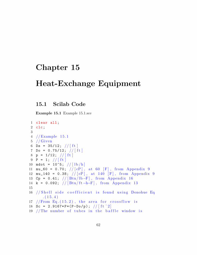
4 // Example 1 5 . 15 // Given6 Ds = 35/12; // [ f t ]7 Do = 0.75/12; // [ f t ]8 p = 1/12; // [ f t ]9 P = 1; // [ f t ]
10 mdot = 10^5; // [ l b /h ]11 mu_60 = 0.70; // [ cP ] , a t 60 [ F ] , from Appendix 912 mu_140 = 0.38; // [ cP ] , a t 140 [ F ] , from Appendix 913 Cp = 0.41; // [ Btu/ lb−F ] , from Appendix 1614 k = 0.092; // [ Btu/ f t −h−F ] , from Appendix 1315
16 // S h e l l s i d e c o e f f i c i e n t i s found u s i n g Donohue Eq. ( 1 5 . 4 )
17 //From Eq . ( 1 5 . 2 ) , the a r ea f o r c r o s s f l o w i s18 Sc = 2.9167*P*(P-Do/p); // [ f t ˆ 2 ]19 //The number o f tube s i n the b a f f l e window i s
62
approx imate l y e q u a l to the f r a c t i o n a l20 // a r ea o f the window f t imes the t o t a l nmber o f
tube s . For a 25 p e r c e n t b a f f l e21 f = 0.1955
22 Nb = f*828;
23 //Nb˜16124 Nb = 161;
25 // Using Eq . ( 1 5 . 1 ) , a r ea o f the b a f f l e window26 Sb = (f*%pi*Ds^2/4) -(Nb*%pi*Do^2/4); // [ f t ˆ 2 ]27 // Using Eq . ( 1 5 . 3 ) , the mass v e l o c i t i e s a r e28 Gc = mdot/Sc; // [ l b / f t ˆ2−h ]29 Gb = mdot/Sb; // [ l b / f t ˆ2−h ]30 Ge = sqrt(Gc*Gb); // [ l b / f t ˆ2−h ]31 // Using Eq . ( 1 5 . 4 )32 ho = k/Do *(0.2*( Do*Ge/(mu_60 *2.42))^0.6*( Cp*mu_60
*2.42/k)^0.33*( mu_60/mu_140)^0.14);// [ Btu/ f t ˆ2−h−F ]
33 disp( ’ Btu/ f t ˆ2−h−F ’ ,ho , ’ The i n d i v i d u a l heat t r a n s f e rc o e f f i c e n t o f benzene i s ’ )
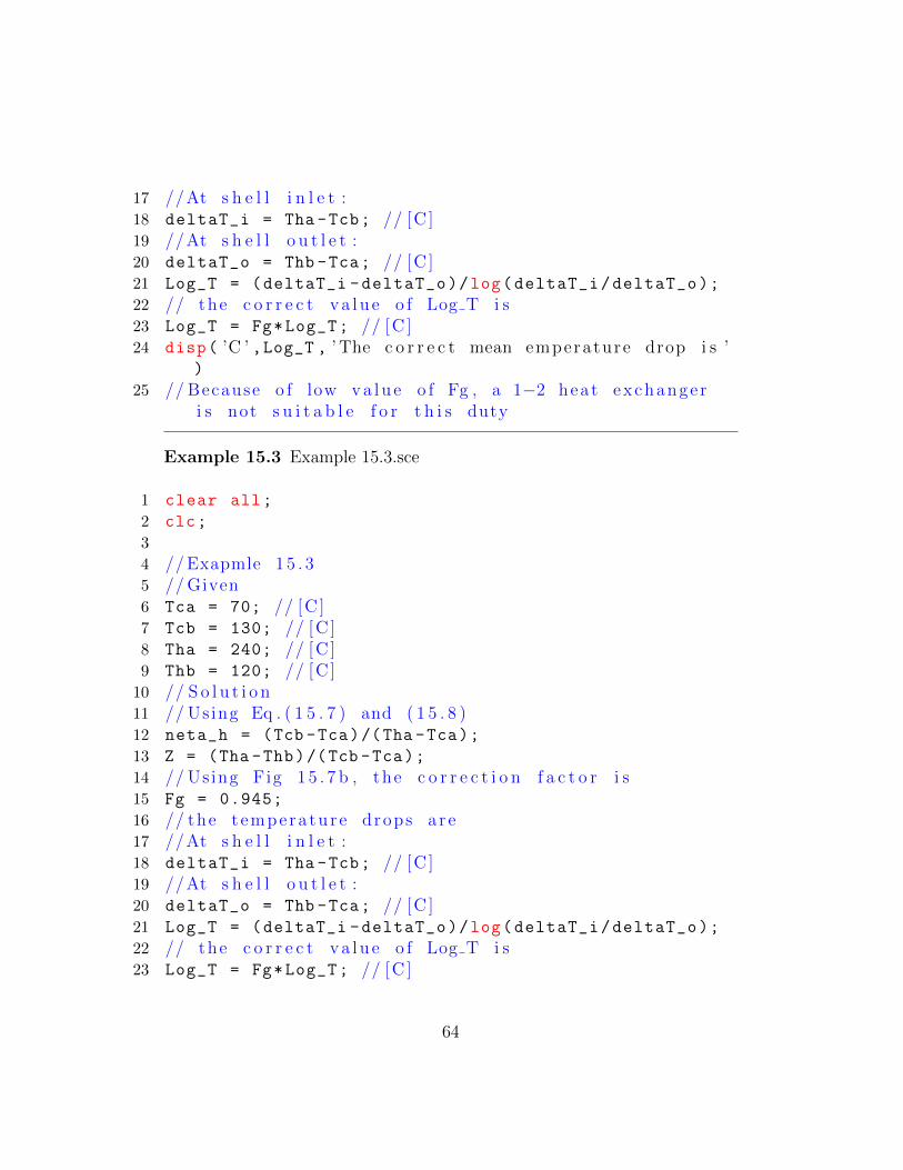
10 // S o l u t i o n11 // Using Eq . ( 1 5 . 7 ) and ( 1 5 . 8 )12 neta_h = (Tcb -Tca)/(Tha -Tca);
13 Z = (Tha -Thb)/(Tcb -Tca);
14 //From Fig 1 5 . 7 a , the c o r r e c t i o n f a c t o r i s found15 Fg = 0.735;
16 // the t empera tu r e drops a r e
63
17 //At s h e l l i n l e t :18 deltaT_i = Tha -Tcb; // [C ]19 //At s h e l l o u t l e t :20 deltaT_o = Thb -Tca; // [C ]21 Log_T = (deltaT_i -deltaT_o)/log(deltaT_i/deltaT_o);
22 // the c o r r e c t v a l u e o f Log T i s23 Log_T = Fg*Log_T; // [C ]24 disp( ’C ’ ,Log_T , ’ The c o r r e c t mean emperature drop i s ’
)
25 // Because o f low v a l u e o f Fg , a 1−2 heat exchange ri s not s u i t a b l e f o r t h i s duty
10 // S o l u t i o n11 // Using Eq . ( 1 5 . 7 ) and ( 1 5 . 8 )12 neta_h = (Tcb -Tca)/(Tha -Tca);
13 Z = (Tha -Thb)/(Tcb -Tca);
14 // Using Fig 1 5 . 7 b , the c o r r e c t i o n f a c t o r i s15 Fg = 0.945;
16 // the t empera tu r e drops a r e17 //At s h e l l i n l e t :18 deltaT_i = Tha -Tcb; // [C ]19 //At s h e l l o u t l e t :20 deltaT_o = Thb -Tca; // [C ]21 Log_T = (deltaT_i -deltaT_o)/log(deltaT_i/deltaT_o);
22 // the c o r r e c t v a l u e o f Log T i s23 Log_T = Fg*Log_T; // [C ]
64
24 disp( ’C ’ ,Log_T , ’ The c o r r e c t mean emperature drop i s ’)
Example 15.4 Example 15.4.sce
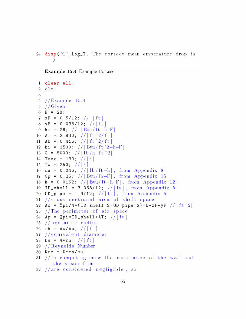
1 clear all;
2 clc;
3
4 // Example 1 5 . 45 // Given6 N = 28;
7 xF = 0.5/12; // [ f t ]8 yF = 0.035/12; // [ f t ]9 km = 26; // [ Btu/ f t −h−F ]10 AT = 2.830; // [ f t ˆ2/ f t ]11 Ab = 0.416; // [ f t ˆ2/ f t ]12 hi = 1500; // [ Btu/ f t ˆ2−h−F ]13 G = 5000; // [ l b /h− f t ˆ 2 ]14 Tavg = 130; // [ F ]15 Tw = 250; // [ F ]16 mu = 0.046; // [ l b / f t −h ] , from Appendix 817 Cp = 0.25; // [ Btu/ lb−F ] , from Appendix 1518 k = 0.0162; // [ Btu/ f t −h−F ] , from Appendix 1219 ID_shell = 3.068/12; // [ f t ] , from Appendix 520 OD_pipe = 1.9/12; // [ f t ] , from Appendix 521 // c r o s s s e c t i o n a l a r ea o f s h e l l space22 Ac = %pi /4*( ID_shell^2-OD_pipe ^2)-N*xF*yF // [ f t ˆ 2 ]23 //The p e r i m e t e r o f a i r space24 Ap = %pi*ID_shell+AT; // [ f t ]25 // h y d r a u l i c r a d i u s26 rh = Ac/Ap; // [ f t ]27 // e q u i v a l e n t d i amete r28 De = 4*rh; // [ f t ]29 // Reynolds Number30 Nre = De*h/mu
31 // In computing mu w the r e s i s t a n c e o f the w a l l andthe steam f i l m
32 // a r e c o n s i d e r e d n e g l i g i b l e , so
65
33 mu_w = 0.0528; // [ l b / f t −h ]34 Npr = mu*Cp/k
35 // Using Fig . 1 5 . 1 7 , the heat t r a n s f e r f a c t o r i s36 jh = 0.0031;
37 ho = jh*Cp*G*(mu/mu_w)^0.14/ Npr ^(2/3); // [ Btu/ f t ˆ2−h−F ]
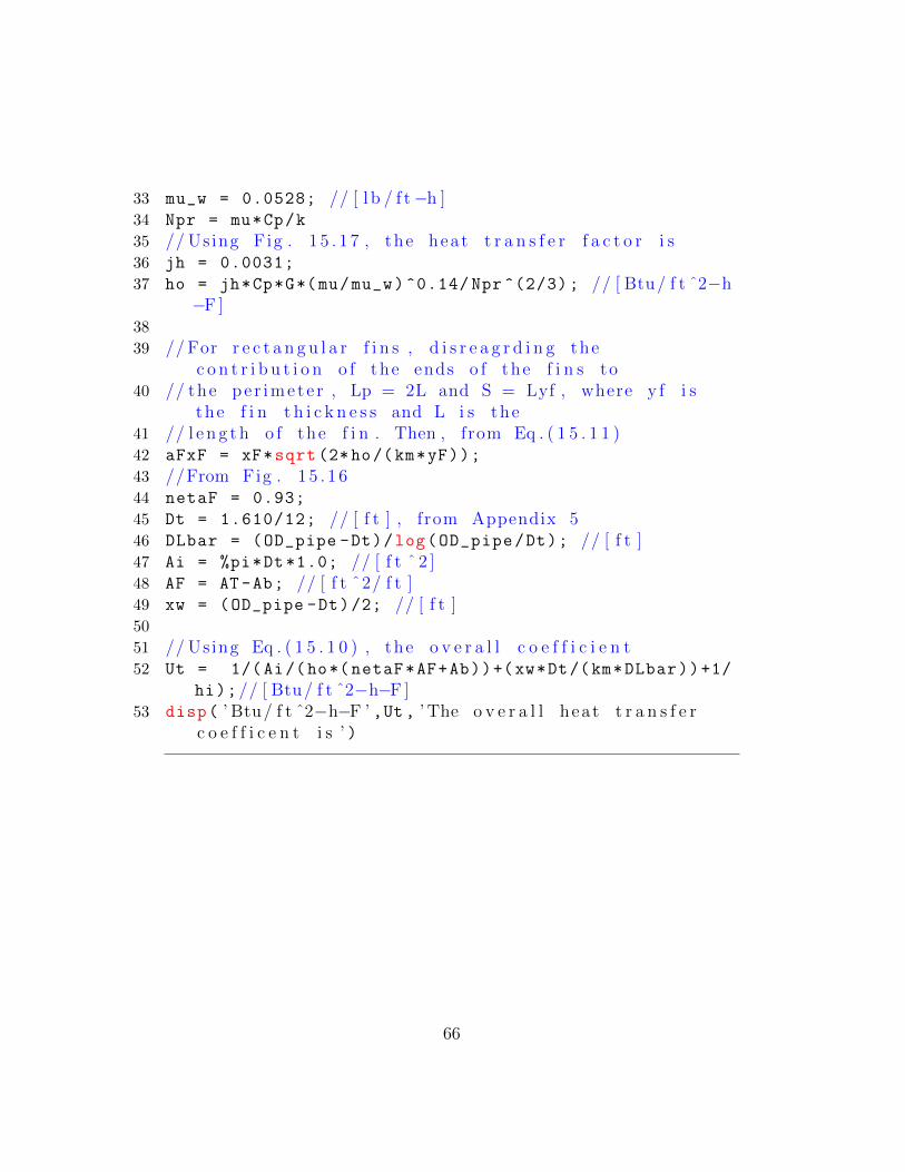
38
39 // For r e c t a n g u l a r f i n s , d i s r e a g r d i n g thec o n t r i b u t i o n o f the ends o f the f i n s to
40 // the pe r ime t e r , Lp = 2L and S = Lyf , where y f i sthe f i n t h i c k n e s s and L i s the
41 // l e n g t h o f the f i n . Then , from Eq . ( 1 5 . 1 1 )42 aFxF = xF*sqrt (2*ho/(km*yF));
43 //From Fig . 1 5 . 1 644 netaF = 0.93;
45 Dt = 1.610/12; // [ f t ] , from Appendix 546 DLbar = (OD_pipe -Dt)/log(OD_pipe/Dt); // [ f t ]47 Ai = %pi*Dt*1.0; // [ f t ˆ 2 ]48 AF = AT-Ab; // [ f t ˆ2/ f t ]49 xw = (OD_pipe -Dt)/2; // [ f t ]50
51 // Using Eq . ( 1 5 . 1 0 ) , the o v e r a l l c o e f f i c i e n t52 Ut = 1/(Ai/(ho*(netaF*AF+Ab))+(xw*Dt/(km*DLbar))+1/
hi);// [ Btu/ f t ˆ2−h−F ]53 disp( ’ Btu/ f t ˆ2−h−F ’ ,Ut , ’ The o v e r a l l heat t r a n s f e r
c o e f f i c e n t i s ’ )
66
Chapter 16
Evaporation
16.1 Scilab Code
Example 16.1 Example 16.1.sce
1 clear all;
2 clc;
3
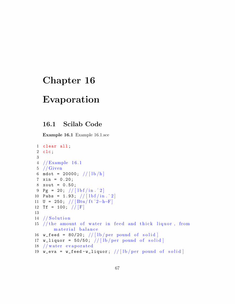
4 // Example 1 6 . 15 // Given6 mdot = 20000; // [ l b /h ]7 xin = 0.20;
8 xout = 0.50;
9 Pg = 20; // [ l b f / i n . ˆ 2 ]10 Pabs = 1.93; // [ l b f / i n . ˆ 2 ]11 U = 250; // [ Btu/ f t ˆ2−h−F ]12 Tf = 100; // [ F ]13
14 // S o l u t i o n15 // the amount o f water i n f e e d and t h i c k l i q u o r , from
m a t e r i a l b a l a n c e16 w_feed = 80/20; // [ l b / per pound o f s o l i d ]17 w_liquor = 50/50; // [ l b / per pound o f s o l i d ]18 // water evapo ra t ed19 w_eva = w_feed -w_liquor; // [ l b / per pound o f s o l i d ]
67
20 // or21 w_eva = w_eva*mdot*xin; // [ l b /h ]22 // Flow raye o f t h i c k l i q u o r i s23 ml_dot = mdot -w_eva // [ l b /h ]24
25 // Steam consumed26 // S i n c e with s t r o n g s o l u t i o n s o f NaOH the heat o f
d i l u t i o n i s not n e g l i g i b l e ,27 // the r a t e o f heat t r a n s f e r i s found from Eq . ( 1 6 . 4 )
and Fig . 1 6 . 8 .28 //The v a p o r i z t i o n t empera tu r e o f the 50 p e r c e n t
s o l u t i o n at a p r e s s u r e o f 100 mmHg29 // i s found as f o l l o w s30 Tb_w = 124; // [ F ] , a t 100 mmHg, from Appendix 731 Tb_s = 197; // [ F ] , from Fig . 1 6 . 832 BPE = Tb_s -Tb_w; // [ F ]33 //From Fig . 1 6 . 8 , the e n t h a l p i e s o f the f e e d and
t h i c k l i q u o r a r e found34 Hf = 55; // [ Btu/ l b ] , 20% s o l i d s , 100 [ F ]35 H = 221; // [ Btu/ l b ] , 50% s o l i d s , 197 [ F ]36 // Enthalpy o f the l e a v i n g water vapor i s found from
the steam t a b l e37 Hv = 1149; // [ Btu/ l b ] , At 197 [ F ] and 1 . 9 3 [ l b f / i n
. ˆ 2 ]38 // Enthalpy o f the vapor l e a v i n g the e v a p o r a t o r39 lambda_s = 939; // [ Btu/ l b ] , At 20 [ l b f / i n . ˆ 2 ] , from
Appendix 740 // Using Eq . ( 1 6 . 4 ) , the r a t e o f heat t r a n s f e r and
steam consumption41 q = (mdot -ml_dot)*Hv + ml_dot*H - mdot*Hf; // [ Btu/h ]42 ms_dot = q/lambda_s; // [ l b /h ]43 disp( ’ l b /h ’ ,ms_dot , ’ steam consumed i s ’ )44 //Economy45 Economy = ml_dot/ms_dot
46 disp(Economy , ’ Economy ’ )47 // Heat ing S u r f a c e48 //The c o n d e n s a t i o n t empera tu r e o f the steam i s 259 [
F ] , the h e a t i n g a r ea r e q u i r e d i s
68
49
50 A = q/(U*(259 -197)) // [ f t ˆ 2 ]51 disp( ’ f t ˆ2 ’ ,A, ’ h e a t i n g a r ea r e q u i r e d i s ’ )
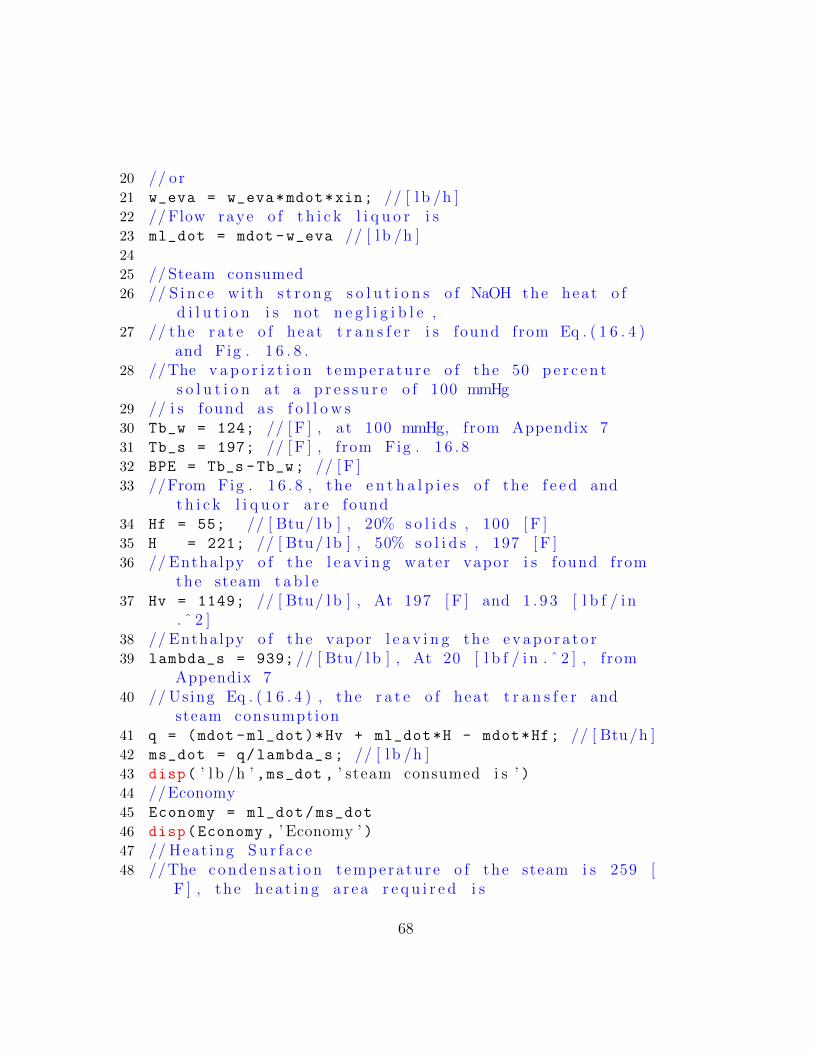
12 // S o l u t i o n13 // Tota l t empera tu r e drop14 delta_T = Ti-Tl; // [C ]15 //From Eq . ( 1 6 . 1 3 ) , the t empera tu r e drops i n s e v e r a l
e f f e c t s w i l l be16 // approx imae ly i n v e r s e l y p r o p o r t i o n a l to the
c o e f i c i e n t s . Thus17 delta_T1 = 1/U1/(1/U1+1/U2+1/U3)*delta_T; // [C ]18 delta_T2 = 1/U2/(1/U1+1/U2+1/U3)*delta_T; // [C ]19 delta_T3 = 1/U3/(1/U1+1/U2+1/U3)*delta_T; // [C ]20 // Consequent ly the b o i l i n g p o i n t s w i l l be21 Tb1 = Ti -delta_T1; // [C ]22 Tb2 = Tb1 -delta_T2; // [C ]23 disp( ’C ’ ,Tb1 , ’ The b o i l i n g p o i n t i n the f i r s t e f f e c t
i s ’ )24 disp( ’C ’ ,Tb2 , ’ The b o i l i n g p o i n t i n the second e f f e c t
i s ’ )
Example 16.3 Example 16.3.sce
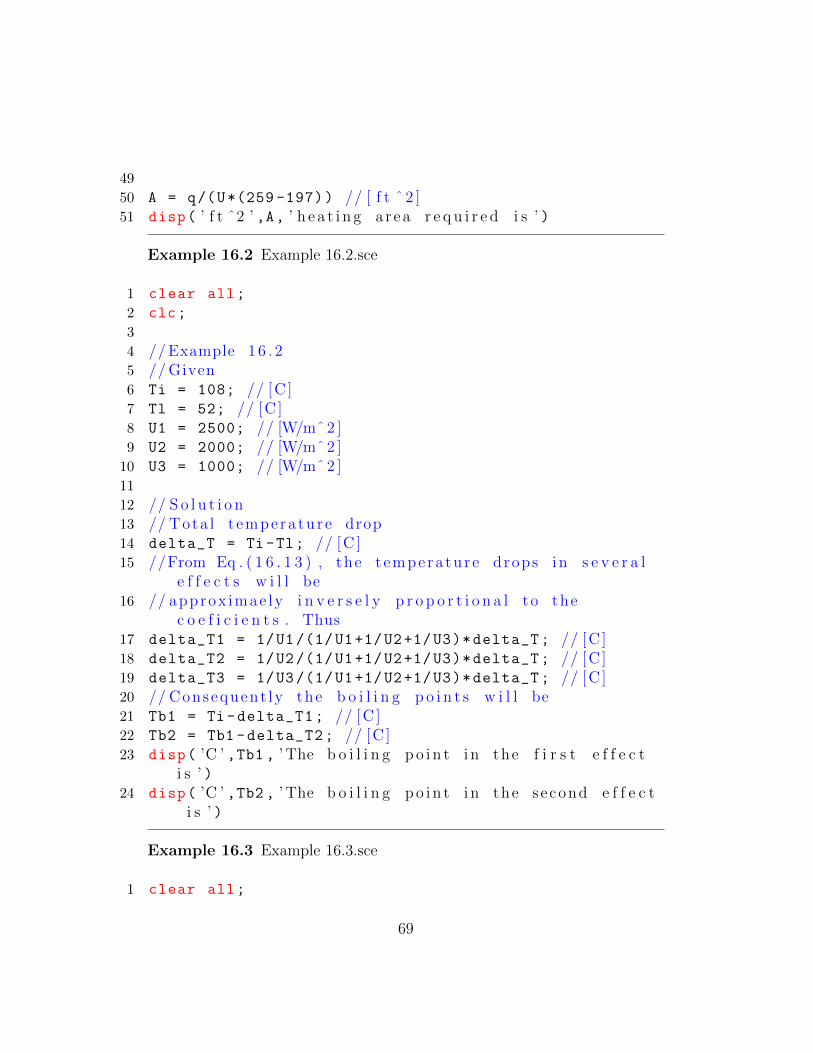
1 clear all;
69
2 clc;
3
4 // Example 1 6 . 35 // Given6 mdot_ft = 60000; // [ l b /h ]7 xin = 0.10;
8 Tin = 180; // [ F ]9 xout = 0.50
10 Ps = 50; // [ l b f / i n . ˆ 2 ]11 Tc = 100; // [ F ]12
13 // S o l u t i o n14 //From Table 1 6 . 215 U1 = 700; // [ Btu/ f t ˆ2−h−F ]16 U2 = 1000; // [ Btu/ f t ˆ2−h−F ]17 U3 = 800; // [ Btu/ f t ˆ2−h−F ]18 //The t o t a l r a t e o f e v a p o r a t i o n i s c a l c u l a t e d from
an o v e r a l l m a t e r i a l b a l a n c e19 // assuming the s o l d s go through the e v a p o r a t o r
w i thout l o s s20 // Table 1 6 . 321 mdot_fs = 6000; // [ l b /h ]22 mdot_fw = 54000; // [ l b /h ]23 mdot_lt = 12000; // [ l b /h ]24 mdot_ls = 6000; // [ l b /h ]25 mdot_lw = 6000; // [ l b /h ]26 w_evap = mdot_ft -mdot_fs; // [ l b /h ]
70
Chapter 17
Equilibrium-Stage Operations
17.1 Scilab Code
Example 17.1 Example 17.1.sce
1 clear all;
2 clc;
3
4 // Example 1 7 . 15 // Given6 yb = 0.30;
7
8 // Let9 Vb = 100; // [ mol ]10 Ace_in = yb*Vb; // [ mol ]11 Air_in = Vb-Ace_in; // [ mol ]12 // 97 p e r c e n t a c e t o n e aborbed , Acetone l e a v i n g i s13 Ace_out = 0.03* Ace_in; // [ mol ]14 ya = Ace_out /( Air_in+Ace_out);
15 // Acetone absorbed16 Ace_abs = Ace_in -Ace_out; // [ mol ]17 // 10 p e r c e n t a c e t o n e i n the l e a v i n g s o l u t i o n and no
a c e t o n e i n the e n t e r i n g o i l18 Lb = Ace_abs /0.1; // [ mol ]19 La = Lb-Ace_abs; // [ mol ]
71
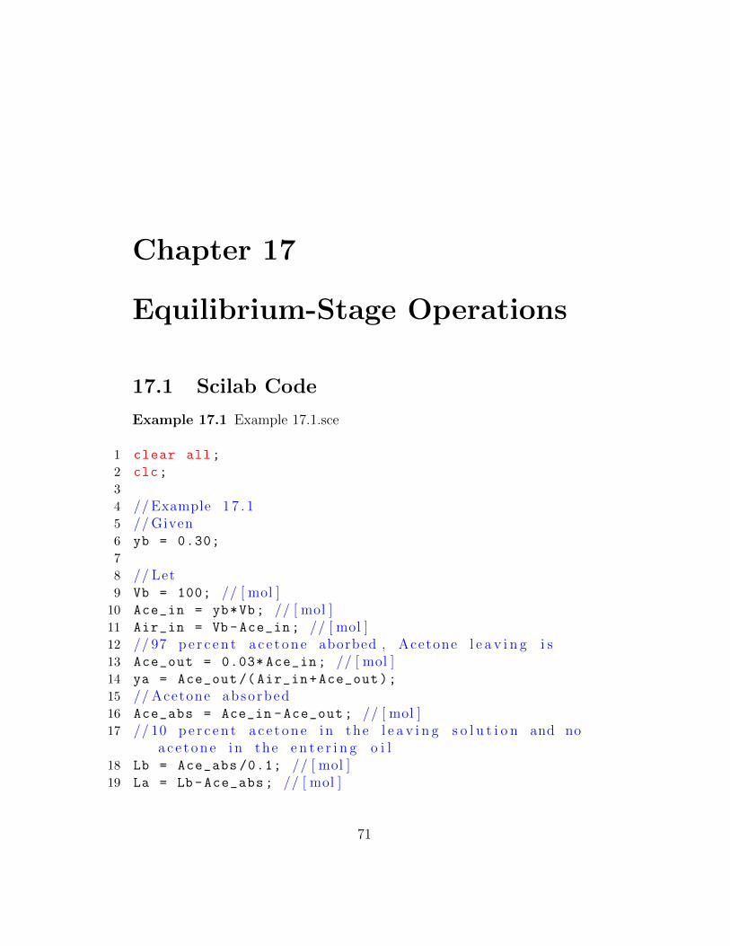
20 //To f i n d out as i n t e r m e d i a t e p o i n t on the o p e r a t i n gl i n e , making an a c e t o n e b a l a n c e
21 // around the top pa r t o f the tower , assuming ap a r t i c u l a r v a l u e o f yV the moles o f
22 // a c e t o n e l e f t i n the gas .23 for i=1:30
24 y(i) = i/(i+Air_in);
25 //The moles o f a c e t o n e l o s t by the gas i n the s e c i o n, must e q u a l to the moles ga ined by // the l i q u i d
34 plot(xe,ye, ’ r ’ )35 xlabel( ’ x ’ )36 ylabel( ’ y ’ )37 legend( ’ Operat ing l i n e ’ , ’ E q u i l i b r i u m l i n e ’ )38 title( ’ Diagram Example 1 7 . 1 ’ )39 //The number o f i d e a l s t a g e s de te rmined from Fig i s
4
72
Figure 17.1: Diagram for Example 17.1
Example 17.2 Example 17.2.sce
1 clear all;
2 clc;
3
4 // Example 1 7 . 25 // Given6 Nreal = 7;
7 VbyL = 1.5;
8 m = 0.8;
9 yb = 0;
73
10 xb_star = 0;
11 // xb =0.1∗ xa ;12
13 // ( a )14 // S t r i p p i n g Facto r15 S = m*VbyL;
16 //From an ammonia ba lance ,17 // ya =0.9∗ xa /VbyL ;18 // Also19 // x a s t a r = ya /m20 // Using Eq . ( 1 7 . 2 8 )21 //N = l n ( ( xa −0.75∗ xa ) / ( 0 . 1 ∗ xa−0) ) / l n ( S )22 N = log (0.25/0.1)/log(S);
23 disp(N, ’ Number o f i d e a l t r a y s r e q u i r e d a r e ’ )24 stage_eff = N/Nreal *100;
25 disp( ’% ’ ,stage_eff , ’ S tage E f f i c i e n c y i s ’ )26
27 // ( b )28 VbyL = 2;
29 S = m*VbyL;
30 //Then ,31 // Let A = ( xa−x a s t a r ) /xb32 A = exp (5.02);
33 // Let ’ f ’ be the f r a c t i o n o f NH3 removed . Then xb =(1− f ) ∗xa .
34 //By a m a t e r i a l b a l a n c e35 //y = L/V∗ ( xa−xb ) = 1/2∗ ( xa−(1− f ) ∗xa )= 1/2∗ f ∗xa36 // x a s t a r = ya /m = 0 . 5∗ f ∗xa / 0 . 8 = 0 . 6 2 5∗ f ∗xa37 //Thus ,38 // xa−x a s t a r = (1 −0.625∗ f ) ∗xa39 // Also ,40 // xa−x a s t a r = 1 0 . 5 9∗ xb = 10.59∗(1 − f ) ∗xa41 // from t h e s e42 f = 0.962
43 disp( ’% ’ ,f, ’ p e r c e n t a g e removal o b t a i n e d i n t h i s c a s ei s ’ )
19 Cp = 0.44; // [ c a l /g−C]20 // ( a )21 //The c o n c e n t r a t i o n s o f f e ed , overhead and bottoms
i n mole f r a c t i o n o f benzene a r e22 xF = (wF_b/Mb)/(wF_b/Mb+((100 - wF_b)/Mt));
23 xD = (wD/Mb)/(wD/Mb+((100 -wD)/Mt));
24 xB = (wB/Mb)/(wB/Mb+((100 -wB)/Mt));
25 //The ave rage m o l e c u l a r we ight o f the f e e d i s26 Mavg = 100/( wF_b/Mb+(100- wF_b)/Mt);
27 // the ave rage heat o f v a p o r i z a t i o n28 lambda_avg = xF*lambda_b +(1-xF)*lambda_t; // [ c a l /g
mol ]29 // Feed r a t e30 F = mdot/Mavg; // [ kg mol/h ]31 // Using Eq . ( 1 8 . 5 ) , by o v e r a l l benzene b a l a n c e32 D = F*(xF-xB)/(xD -xB); // [ kg mol/h ]33 B = F-D; // [ kg mol/h ]34 disp( ’ r e s p e c t i v e l y ’ , ’ kg mol/h ’ ,B, ’ kg mol/h ’ ,F, ’ the
mole o f overhead and bottom p r o d u c t s a r e ’ )35
36
37 // ( b ) Deteminat ion o f number o f i d e a l p l a t e s andp o s i t i o n o f f e e d p l a t e
38 // ( i )
77
39 // Using Fig . 1 8 . 1 640 // Drawing the f e e d l i n e with f = 0 on e q u i l i b r i u m
diagram ,41 // P l o t t i n g the o p e r a t i n g l i n e s with i n t e r c e p t from
Eq . ( 1 8 . 1 9 ) i s 0 . 2 1 642 //By c o u n t i n g the r e c t a n g u l a r s t e p s i t i s found that
, b e s i d e s the r e b o i l e r ,43 // 11 i d e a l p l a t e s a r e neded and f e e d shou ld be
i n t r o d u c e d on the 7 th p l a t e from44 // the top .45
46 // ( i i )47 //The l a t e n t heat o f v a p o r i z a t i o n o f the f e e d48 lambda = lambda_avg/Mavg; // [ c a l /g ]49 // Using Eq . ( 1 8 . 2 4 )50 q = 1+Cp*(TB-TF)/lambda;
51 //From Eq . ( 1 8 . 3 1 )52 slope = -q/(1-q);
53 //From Fig . 1 8 . 1 754 // I t i s found tha t a r e b o i l e r and 10 i d e a l p l a t e s
a r e needed and f e e d i s to be i n t r o d u c e d55 // on the f i f t h p l a t e56
57 // ( i i i )58 q = 1/3;
59 slope = -q/(1-q);
60 //From Fig . 1 8 . 1 861 // I t c a l l s f o r a r e b o i l e r and 12 p l a t e s , with the
f e e d e n t e r i n g on the 7 th p l a t e62
63 // ( c )64 // vapor f l o w i n the r e c t i f y i n g s e c t i o n i s65 V = 4.5*D; // [ kg mol/h ]66 lambda_s = 522; // [ c a l /g ] , From Appendix 767 q = [1, 1.37, 0.333]
68 // Using Eq . ( 1 8 . 2 7 )69 Vbar = V-F*(1-q)
70 // Using Eq . ( 1 8 . 3 2 ) , steam r e q u i r e d
78
71 ms_dot = lambda_t/lambda_s*Vbar; // [ kg /h ]72 disp( ’ r e s p e c t i v e l y ’ , ’ kg /h ’ ,ms_dot (3), ’ kg /h ’ ,ms_dot
(2), ’ kg /h ’ ,ms_dot (1), ’ the steam consumption i nthe above t h r e e c a s e s i s ’ )
73
74
75 // ( d )76 Tw1 = 25; // [C ]77 Tw2 = 40; // [C ]78 //The c o o l i n g water needed i s same i n a l l c a s e s ,
Us ing Eq . ( 1 8 . 3 3 )79 mw_dot = V*lambda_t /(Tw2 -Tw1); // [ kg /h ]80 rho_25 = 62.24*16.018; // [ kg /mˆ 3 ]81 vw_dot = mw_dot/rho_25; // [mˆ3/h ]82 disp( ’mˆ3/h ’ ,vw_dot , ’ c o o l i n g water needed i s ’ )
Example 18.3 Example 18.3.sce
1 clear all;
2 clc;
3
4 // Example 1 8 . 35 // Given6 mdot = 30000; // [ kg /h ]7 wF_b = 40;
8 wD = 97;
9 wB = 2;
10 R = 3.5;
11 lambda_b = 7360; // [ c a l /g mol ]12 lambda_t = 7960; // [ c a l /g mol ]13 alpha = 2.5;
19 Cp = 0.44; // [ c a l /g−C]20 // S o l u t i o n
79
21 xF = (wF_b/Mb)/(wF_b/Mb+((100 - wF_b)/Mt));
22 xD = (wD/Mb)/(wD/Mb+((100 -wD)/Mt));
23 xB = (wB/Mb)/(wB/Mb+((100 -wB)/Mt));
24 //The ave rage m o l e c u l a r we ight o f the f e e d i s25 Mavg = 100/( wF_b/Mb+(100- wF_b)/Mt);
26 // the ave rage heat o f v a p o r i z a t i o n27 lambda_avg = xF*lambda_b +(1-xF)*lambda_t; // [ c a l /g
mol ]28 // Feed r a t e29 F = mdot/Mavg; // [ kg mol/h ]30 // Using Eq . ( 1 8 . 5 ) , by o v e r a l l benzene b a l a n c e31 D = F*(xF-xB)/(xD -xB); // [ kg mol/h ]32 B = F-D; // [ kg mol/h ]33 // Using Table 1 8 . 3 , i n a l l t h r e e c a s e s r e s p e c t i v e l y34 xprime = [0.44 ,0.521 ,0.3];
20 //By o v e r a l l e t h o n a l b a l a n c e21 ya = Lbar/Vbar*(xa-xb)+ yb
22 // Using Eq . ( 1 7 . 2 7 ) , As both o p e r t i n g l i n e s ande q u i l i b r i u m l i n e s a r e s t r a i g h t
23 N = log((ya-ya_star)/(yb-yb_star))/log((yb_star -
ya_star)/(yb-ya));
24
25 disp(N, ’ I d e a l p l a t e s needed a r e ’ )
Example 18.6 Example 18.6.sce
1 clear all;
2 clc;
3
4 // Example 1 8 . 65 // Given6 xF = 0.40;
7 P = 1; // [ atm ]8 D = 5800; // [ kg /h ]9 R = 3.5;
10 LbyV = R/(1+R);
11 // S o l u t i o n12 // P h y s i c a l p r o p e r t i e s o f methanol13 M = 32;
81
14 Tnb = 65; // [C ]15 rho_v = M*273/(22.4*338); // [ kg / ˆ 3 ]16 rho_l_0 = 810; // [ kg /mˆ 3 ] , At 0C, from Perry ,
Chemical Eng inee r s ’ Handbook17 rho_l_20 = 792; // [ kg /mˆ 3 ] , At 20C, from Perry ,
Chemical Eng inee r s ’ Handbook18 rho_l = 750; // [ kg /mˆ 3 ] , At 65C19 sigma = 19; // [ dyn/cm ] , from Lange ’ s Handbook o f
Chemistry20 // ( a )21 // Vapor v e l o c i t y and column d iamete r22 // Using Fig . 1 8 . 2 8 , the a b s c i s s a i s23 abscissa = LbyV*(rho_v/rho_l)^(1/2);
24 // f o r 18− i n . p l a t e s p a c i n g25 Kv = 0.29;
26 // A l l owab l e vapor v e l o c i t y27 uc = Kv*((rho_l -rho_v)/rho_v)^(1/2) *( sigma /20) ^(0.2)
; // [ f t / s ]28 // Vapor f l o w r a t e29 V = D*(R+1) /(3600* rho_v); // [mˆ3/ s ]30 // Cross s e t i o n a l a r ea o f the column31 Bubbling_area = V/2.23; // [mˆ 2 ]32 // I f the bubble a r ea i s 0 . 7 o f the t o t a l column ar ea33 Column_area = Bubbling_area /0.7; // [mˆ 2 ]34 //Column d iamete r35 Dc = sqrt (4* Column_area/%pi); // [m]36 disp( ’ r e s p e c t i v e l y ’ , ’m ’ ,Dc , ’ and ’ , ’ f t / s ’ ,uc , ’ the
a l l o w a b l e v e l o c i t y and colmn d iamete r a r e ’ )37
38 // ( b )39 // P r e s s u r e drop :40 // Area o f one u n i t o f t h r e e h o l e s on a t r a n g u l a r
3/4− i n . p i t c h i s41 // 1/2∗3/4∗ (3/4∗ s q r t ( 3 / 2 ) ) i n . ˆ 2 . The h o l e a r ea i n
t h i s s e c t i o n ( h a l f a h o l e ) i s42 // 1/2∗%pi / 4∗ ( 1/ 4 ) ˆ2 i n . ˆ 2 . Thus the h o l e a r ea i s %pi
/128∗64/9∗ s q r t ( 3 ) , o r 1 0 . 0 8 p e r c e n t43 // o f the bubb l ing a r ea .
82
44 // Vapor v e l o c i t y through h o l e s :45 uo = 2.23/0.1008; // [m/ s ]46 // Using Eq . ( 1 8 . 5 8 ) ,47 //From Fig . 1 8 . 2 748 Co = 0.73;
49 hd = 51.0*uo^2* rho_v/(Co^2* rho_l); // [mm methanol ]50 // Head o f l i q u i d on p l a t e :51 // Weir h e i g h t52 hw = 2*25.4; // [mm]53 // He ight o f the l i q u i d above we i r :54 // Assuming the downcomer a r ea i s 15 p e r c e n t o f the
column55 // a r ea on each s i d e o f th column . From Perry , the
chord56 // l e n g t h f o r sucha segmenta l downcomer i s 1 . 6 2 t imes
the r a d i u s57 // o f the colmn , so58 Lw = 1.62*2.23/2; // [m]59 // L iq iud Flow r a t e :60 qL = D*(R+1)/(rho_l *60); // [mˆ3/ min ]61 //From Eq . ( 1 8 . 6 0 )62 how = 43.4*( qL/Lw)^(2/3) // [mm]63 //From Eq . ( 1 8 . 5 9 ) , with64 beeta = 0.6;
65 hI = beeta*(hw+how); // [mm]66 // Tota l h e i g h t o f l i q u i d , from Eq . ( 1 8 . 6 2 )67 hT = hd+hI; // [mm]68 disp( ’mm methanol ’ ,hT , ’ p r e s s u r e drop per p l a t e i s ’ )69
70 // ( c )71 // Froth h e i g h t i n th downcomer :72 // Using Eq . ( 1 8 . 6 2 ) . , E s t imat ing73 hf_L = 10; // [mm methanol ]74 //Then ,75 Zc = (2*hI)+hd+hf_L; // [mm]76 // from Eq . ( 1 8 . 6 3 )77 Z = Zc/0.5; // [mm]78 disp( ’mm methanol ’ ,Z, ’ Froth h e i g h t i n the downcomer
83
i s ’ )
Example 18.7 Example 18.7.sce
1 clear all;
2 clc;
3
4 // Example 1 8 . 75 // Given6 xF = 0.40;
7 P = 1; // [ atm ]8 D = 5800; // [ kg /h ]9 R = 3.5;
10 LbyV = R/(1+R);
11 // S o l u t i o n12 // P h y s i c a l p r o p e r t i e s o f methanol13 M = 32;
14 Tnb = 65; // [C ]15 rho_v = M*273/(22.4*338); // [ kg / ˆ 3 ]16 rho_l_0 = 810; // [ kg /mˆ 3 ] , At 0C, from Perry ,
Chemical Eng inee r s ’ Handbook17 rho_l_20 = 792; // [ kg /mˆ 3 ] , At 20C, from Perry ,
Chemical Eng inee r s ’ Handbook18 rho_l = 750; // [ kg /mˆ 3 ] , At 65C19 sigma = 19; // [ dyn/cm ] , from Lange ’ s Handbook o f
Chemistry20 // ( a )21 // Vapor v e l o c i t y and column d iamete r22 // Using Fig . 1 8 . 2 8 , the a b s c i s s a i s23 abscissa = LbyV*(rho_v/rho_l)^(1/2);
24 // f o r 18− i n . p l a t e s p a c i n g25 Kv = 0.29;
26 // A l l owab l e vapor v e l o c i t y27 uc = Kv*((rho_l -rho_v)/rho_v)^(1/2) *( sigma /20) ^(0.2)
/(3.2825112); // [ f t / s ]28 //From Eq . ( 1 8 . 7 1 ) , the F f a c t o r i s29 F = uc*sqrt(rho_v);
30 disp(F, ’ the v a l u e o f F f a c t o r i s ’ )
22 // In Eq . ( 1 9 . 1 2 ) , the r i g h t hand s i d e o f the e q u a t i o nbecomes
23 RHS = (xF./(f*(K-1)+1));
24 RHS2 = sum(RHS)
25 disp( ’C ’ ,Td , ’ f l a s h t empera tu re i s ’ );26 disp( ’ p e r c e n t ’ ,RHS(3), ’ n−oc taneexane ’ , ’ p e r c e n t ’ ,RHS
(2), ’ n−heptane ’ , ’ p e r c e n t ’ ,RHS(1), ’ n−hexane ’ , ’Compos i t ion o f the l i q u i d product i s ’ );
27 y = RHS.*K;
28 disp( ’ p e r c e n t ’ ,y(3), ’ n−oc tane ’ , ’ p e r c e n t ’ ,y(2), ’ n−heptane ’ , ’ p e r c e n t ’ ,y(1), ’ n−hexane ’ , ’ Compos i t iono f the vapor product i s ’ );
29
30 // ( b )31 //To de t e rmine the t empera tu re o f the f e e d b e f o r e
f l a s h i n g ,32 // an en tha lpy b a l a n c e i s made u s i n g 105 C as the
r e f e r e n c e t empera tu r e .33 //The h e a t s o f v a p o r i z a t i o n at 105 C and the ave rage
heat c a p a c i t i e s o f the34 // l i q u i d from 105 to 200 C a r e o b t a i n e d from the
l i t e r a t u r e .35 Cp = [62,70 ,78] ’; // [ c a l /mol−C] , Cp ( 1 ) = n−hexane ,
Cp ( 2 ) = n−heptane , and Cp ( 3 ) = n−oc tane36 delta_Hv = [6370 ,7510 ,8560] ’; // [ c a l /mol ] , d e l t a h v
( 1 ) = n−hexane , d e l t a h v ( 2 ) = n−heptane , andd e l t a h v ( 3 ) = n−oc tane
37 // Based on l i q u i d at 105 C, the e n t h a l p i e s o f theproduct a r e
38 H_vapor = f*sum((y.* delta_Hv)) // [ c a l ]39 H_liquid = 0;
40 // For the f e e d41 Cp_bar = sum(xF.*Cp) // [ c a l /mol−C]42 T0 = H_vapor/Cp_bar+Td;
43 disp( ’C ’ ,T0 , ’ p r e h e a t t empera tu r e i s ’ )
87
Example 19.3 Example 19.3.sce
1 clear all;
2 clc;
3
4 // Example 1 9 . 35 // Given6 xF = [0.33 ,0.37 ,0.30] ’; // [ mole f r a c t i o n ] xF ( 1 ) = n−
hexane , xF ( 2 ) = n−heptane , and xF ( 3 ) = n−oc tane7 P = 1.2; // [ atm ]8 f = 0.60;
9 xD_hex = 0.99; // [ mole f r a c t i o n ]10 xB_hex = [0.01]; // [ mole f r a c t i o n ]11 K(1) = 2.68/P;
12 K(2) = 1.21/P;
13 K(3) = 0.554/P;
14 // S o l u t i o n15 //The n−hexane i s the l i g h t key (LK) , the n−hepane i s
the heavy key (HK) , and the16 //n−oc tane i s a heavy nonkey (HNK)17 // Aply ing mass b a l a n c e and assuming no n−oc tane and
0 . 9 9 mole f r a c t i o n n−hexane i n the18 // d i s t i l l a t e .19 // B a s i s :20 F = 100; // [ mol/h ]21 //B+D = 1 0 0 ;22 // For hexane ,23 //F∗xF = D∗xD+B∗xB24 // from the above two e q u a i t o n25 A_BD = [1,1; xD_hex xB_hex ];
26 B_BD = [F;F*xF(1)];
27 //A BD∗x BD = B BD28 x_BD = inv(A_BD)*B_BD;
29 D = x_BD (1);
30 B = x_BD (2);
31 xD = [0.99 ,0.01 ,0.0] ’;
88
32 xB = [0.01 ,0.544 ,0.446] ’;
33 comp_D = xD.*D;
34 comp_B = xB.*B;
35
36 disp( ’ mol /h ’ ,comp_D (3), ’ n−oc tane ’ , ’ mol /h ’ ,comp_D (2),’ n−heptane ’ , ’ mol /h ’ ,comp_D (1), ’ n−hexane ’ , ’ Thec o m p o s i t i o n o f the overhead product i s ’ );
37 disp( ’ mol /h ’ ,comp_B (3), ’ n−oc tane ’ , ’ mol /h ’ ,comp_B (2),’ n−heptane ’ , ’ mol /h ’ ,comp_B (1), ’ n−hexane ’ , ’ Thec o m p o s i t i o n o f the bottom product i s ’ );
38
39 //To f i n d out minimum number o f p l a t e s , u s i n g Eq. ( 1 9 . 1 3 ) [ Fenske Equat ion ]
40 // u s i n g r e l a t i v e v o l a t i v i t y o f the l i g h t key to theheavy key , which i s the
41 // r a t i o o f the K f a c t o r s . The K v a l u e s at the f l a s htemperatue a r e taken from Example 1 9 . 2
42 alpha_LK_HK = K(1)/K(2);
43 Nmin = log((xD(1)/xD(2))/(xB(1)/xB(2)))/log(
alpha_LK_HK) -1;
44 disp( ’ p l u s a r e b o i l e r ’ ,Nmin , ’ The minimum number o fi d e a l s t a g e s i s ’ );
Example 19.4 Example 19.4.sce
1 clear all;
2 clc;
3
4 // Example 1 9 . 45 // Given6 //x ( 1 ) = n−pentane , x ( 2 ) = n−hexane , x ( 3 ) = n−
heptane and x ( 4 ) = n−oc tane7 //xF = feed , xD = d i s t i l l a t e and xB = bottom8 xF = [4 40 50 6] ’./100 // [ mole f r a c t i o n ]9 P = 1; // [ atm ]
10 xD1 (2) = 0.98;
11 xD1 (3) = 0.01;
12
89
13 // S o l u t i o n14 //The keys a r e n−hexane and n−heptane , and the o t h e r
components a r e15 // s u f f i c i e n t l y d i f f e r e n t i n v o l a t i l i t y to be
d i s t r i b u t e d .16 // B a s i s :17 F = 100; // [ mol ]18 xD1 (1) = 1;
31 //A = (RD−RDm) /RD+132 // from Fig . 1 9 . 533 N = (Nmin +0.41) /(1 -0.41);
34
35 disp(N, ’ The number o f i d e a l p l a t e r e q u i r e d a r e ’ )
92
Chapter 20
Leaching and Extraction
20.1 Scilab Code
Example 20.1 Example 20.1.sce
1 clear all;
2 clc;
3
4 // Example 20 15 // Given6 Fin = 2*10^3; // [ kg / day ]7 //w( 1 ) = p a r a f f i n wax , w( 2 ) = paper pulp8 wi = [0.25 ,0.75] ’; // [ w ieght p e r c e n t ]9
10 // S o l u t i o n11 // Using c o n v e n i e n t u n i t s i n Eq . ( 1 7 . 2 4 )12 //As the r a t i o o f k e r o s e n e to pulp i s cons tant , f l o w
r a t e s shou ld be13 // e x p r e s s e d i n pounds o f k e r o s e n e . Then , a l l the
c o n c e n t r a t i o n s must14 // be i n pound o f wax− f r e e k e r o s e n e . The u n e x t r a c t e d
paper had no k e r o s e n e15 // so the f i r s t c e l l must be t r e a t e d s e p a r a t e l y .16 // R e f e r i n g to the Fig . 2 0 . 317 // B a s i s :
93
18 F = 100; // [ l b wax + kero s ene− f r e e pulp ]19 //By making a mass b a l a n c e ove r wax20 // wax in = F∗ ( wi ( 1 ) / wi ( 2 ) )+ 0 . 0 0 0 5∗ s ( s i s the wax
input with s o l v e n t )21 // wax out = F ∗ ( 0 . 0 0 2 ) +(s −200) ∗0 . 0 522 // by wax in = wax out23 s_in = (33.33+9.8) /(0.05 -0.0005); // [ l b ]24 //The c o n c e n t r a t i o n o f t h i s s t ream i s , t h e r e f o r e25 s_out = 200; // [ l b ]26 s_stsol = s_in -s_out; // [ l b ]27 wax_sol = s_stsol *0.05; // [ l b ]28 //The c o n c e n t r a t i o n i n the unde r f l ow to the second
u n i t e q u a l s tha t29 // o f the o v e r f l o w from the f i r s t s tage , o r 0 . 0 5 l b
o f wax per pound30 // o f k e r o s e n e . The wax i n the unde r f l ow to u n i t 2 i s31 wax_uflow_2 = s_out *0.05; // [ l b ]32 wax_oflow_21 = wax_uflow_2+wax_sol -F*(wi(1)/wi(2))
// [ l b ]33
34 //The c o n c e n t r a t i o n s o f t h i s s t ream i s , t h e r e f o r e ,35 ya = wax_oflow_21 /871;
36 yastar = 0.05;
37 xa = yastar;
38 ybstar = 0.2/ s_out;
39 xb = ybstar;
40 yb = 0.0005;
41
42 // S i n c e 1 s t a g e has a l r e a d y ben taken i n t o account ,43 //Eq . ( 1 7 . 2 4 ) , w i l l g i v e N−1 s t a g e s , Hence44 N = log((yb-ybstar)/(ya-yastar))/log((yb-ya)/(ybstar
-yastar));
45 disp(N+1, ’ The t o t a l number o f i d e a l s t a g e s i s ’ );
Example 20.2 Example 20.2.sce
1 clear all;
2 clc;
94
3
4 // Example 2 0 . 25 // Given6 F = 1000; // [ kg ]7 solv_O = 10; // [ kg ]8 solv_B = 655; // [ kg ]9 w_out = 60; // [ kg ]10 // S o l u t i o n11 // Let s o l u t i o n r e t a i n e d i s SR , from Table 2 0 . 112 SR =
14 // Let x and y be the mass f r a c t i o n o f o i l i n theunde r f l ow and
15 // o v e r f l o w s o l u t i o n s .16
17 //At the s o l v e n t i n l e t ,18 Vb = solv_O + solv_B; // [ kg s o l u t i o n /h ]19 yb = solv_O/Vb;
20 err = 1;
21 i = 1;
22 sr = SR(2);
23 xb1 = 0.0;
24 while(err >0.001)
25 Lb = sr*F;
26 xbnew = w_out/Lb;
27 err = abs(xb1 -xbnew);
28 xb1 = xbnew;
29 sr = SR(i)+(xb1 -xb(i))/(xb(i+1)-xb(i))*(SR(i+1)-SR
(i));
30 i =i+1;
31 end
32 Lb = sr*F;
33 // Benzene i n the unde r f l ow at Lb i s34 Underlow_B = Lb -w_out; // [ kg s o l u t i o n s /h ]35
36 // At the s o l i d i n l e37 La = 400+25; // [ kg s o l u t i o n s /h ]
95
38 xa = 400/La;
39 w_in = 10+400; // [ kg /h ]40 Extract_O = w_in - w_out; // [ kg /h ]41 Extract_B = 655+25 -447; // [ kg /h ]42 Va = Extract_O+Extract_B; // [ kg /h ]43 ya = Extract_O/Va;
44
45 //The answers to p a r t s ( a ) to ( d ) a r e46 // ( a )47 disp(ya, ’ The c o n c e n t r a t i o n o f s t r o n g s o l u t i o n i s ’ );48 // ( b )49 disp(xb1 , ’ The c o n c e n t r a t i o n o f the s o u l t i o n a d h e r i n g
to the e x t r a c t e d s o l i d s i s ’ );50 // ( c )51 disp( ’ kg /h ’ ,Lb , ’ The mass o f s o l u t i o n l e a v i n g with
the e x t r a c t e d meal i s ’ );52 // ( d )53 disp( ’ kg /h ’ ,Va , ’ The mass o f e x t r a c t i s ’ );54
55 // ( e )56 //To de t e rmine an i n t e r m e d i a t e p o i n t on the
o p e r a t i n g l i n e , choos ing ,57 xn = 0.5;
58 // S o u l i o n r e t a i n e d59 Ln = 0.571*F; // [ kg /h ]60 //By o v e r a l l ba lance , Eq . ( 2 0 . 1 )61 V_n_1 = Va+Ln -La; // [ kg /h ]62 //By o i l b a l a n c e63 y_n_1 = (Ln*xn+Va*ya-La*xa)/V_n_1;
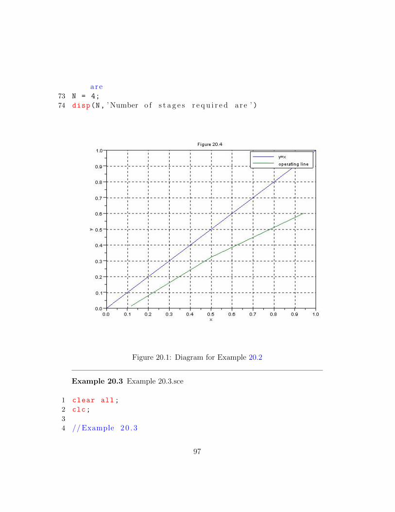
64 y =0:0.1:1;
65 x = y;
66 plot(x,y,[xb1 ,xn ,xa],[yb ,y_n_1 ,ya])
67 xgrid()
68 xlabel( ’ x ’ )69 ylabel( ’ y ’ )70 title( ’ F i gu r e 2 0 . 4 ’ )71 legend( ’ y=x ’ , ’ o p e r a t i n g l i n e ’ )72 // Using F igu r e 2 0 . 4 , number o f i d e a l s t a g e s r e q u i r e d
96
a r e73 N = 4;
74 disp(N, ’ Number o f s t a g e s r e q u i r e d a r e ’ )
Figure 20.1: Diagram for Example 20.2
Example 20.3 Example 20.3.sce
1 clear all;
2 clc;
3
4 // Example 2 0 . 3
97
5 // Given6 T = 25; // [C ]7 //x ( 1 ) = Acetone , x ( 2 )= water and x ( 3 )= MIK8 //F = f e e d9 xF = [0.40, 0.60 ,0.0] ’;
10 xMIK_i = [0.0 ,0.0 ,1.0] ’;
11
12 // S o l u t i o n13 // Using data from Fig . 2 0 . 1 0 , to p l o t e q u i l i b r i u m
curve14 // Fig . 2 0 . 1 3 .15 // B a s i s :16 F = 100; // [ mass u n i t s /h ]17 // Let n = mass f l o w r a t e o f H2O i n e x t a r c t18 //m = mass f l o w r a t e o f MIK i n r a f f i n a t e19 // For 99 p e r c e n t r e c o v e r y o f A, the e x t a r c t has20 E_A = 0.99* xF(1)*F;
21 //And the R a f f i n a t e has22 R_A = xF(1)*F-E_A;
23 //The t o t a l f l o w s a r e24 //At the top ,25 //La = F = 40∗A+60∗H2O26 //Va = 3 9 . 6∗A+n∗H20+(100−m) ∗MIK = 1 3 9 . 6 + n−m27 //At the bottom ,28 Vb = 100; // MIK29 //Lb = 0 . 4∗A+(60−n ) ∗H2O+m∗MIK = 6 0 . 4 +m−n30 // S i n c e n and m a r e s m a l l and tend to c a n c e l i n the
summatios f o r Va and La ,31 // the t o t a l e x t r a c t f l o w Va i s about 140 , which
would make32 yA_a = 39.6/140;
33 xA = 0.4/60;
34 //From Fig 2 0 . 1 0 , f o r35 yA = 0.283, yH2O = 0.049
36 xA = 0.007, xMIK = 0.02
37 nm = [6;2];
38 err = 1;
39 while(err >0.1)
98
40 nmold = nm;
41 nm(1) = yH2O/(1-yH2O)*(39.6+100 - nm(2));
42 nm(2) = xMIK/(1-xMIK)*(0.4+60 -nm(1));
43 err = norm(nm-nmold);
44 end
45 n = nm(1);
46 m = nm(2);
47 Va = 139.6+n-m;
48 yA_a = 39.6/Va;
49 Lb = 60.4+m-n;
50 xA_b = 0.4/Lb;
51
52 // For an i n t e r m e d i a t e p o i n t on the o p e r a t i n g l i n e ,p i c k i n g
53 yA = 0.12;
54 //From Fig . 2 0 . 1 0 ,55 yH2O = 0.03;
56 yMIK = 0.85;
57 // S i n c e the r a f f i n a t e phase has on ly 2 to 3 pecen tMIK, assuming
58 // tha t the amount o f MIK i n the e x t r a c t i s 100 , thesame as the s o l v e n t
59 // f e d :60 V = 100/ yMIK;
61 //By an o v e r a l l b a l a n c e from the s o l v e n t i n l e t (bottom ) to the i n t e r m e d i a t e
62 // po int ,63 xb = xA_b;
64 L = Lb+V-Vb;
65 yb = 0;
66 //A b a l a n c e on A ove r the same s e c t i o n g i v e s xA ;67 xA = (0.4+117.6*0.12 -0)/L;
68 // For xA and xMIK = 0 . 0 3 , A b a l a n c e on MIK from thes o l v e n t
69 // i n l e t to the i n t e r m e d i a t e p o i n t g i v e s70 V_revised = 101.1/0.85;
77 xlabel( ’ x ’ )78 ylabel( ’ y ’ )79 title( ’ F i gu r e 2 0 . 1 3 ’ )80 legend( ’ y=x ’ , ’ o p e r a t i n g l i n e ’ )81
82 //From Fig . 2 0 . 1 383 disp (3.4, ’ Number o f s t a g e s ’ )
Figure 20.2: Diagram for Example 20.3
100
101
Chapter 21
Principles of Diffusion andMass Transer between Phases
21.1 Scilab Code
Example 21.1 Example 21.1.sce
1 clear all;
2 clc;
3
4 // Exapmle 2 1 . 15 // Given6 yA = 0.20;
7 yAi = 0.10;
8
9 // S o l u t i o n10 // ( a )11 // Let A = Dv∗ rho M/BT12 A = 1; // assumed13
14 // Using Eq . ( 2 1 . 1 9 ) , f o r e u i l m o l a l d i f f u s i o n ,15 JA = A*(yA-yAi);
16 //Form Eq . ( 2 1 . 2 4 ) , f o r one way d i f f u s i o n ,17 NA = A*log((1-yAi)/(1-yA));
18 NAbyJA = NA/JA;
102
19 disp( ’ In t h i s c a s e the t r a n s f e r r a t e with one−wayd i f f u s i o n i s ’ ,NAbyJA -1, ’ p e r c e n t g r e a t e r than tha twith e q u i m o l a l d i f f u s i o n ’ );
20
21 // ( b )22 //Whwn, b = BT/223 A = A*2;
24 yA = 1-exp(NA/2)*(1-yA)
25 disp(yA, ’ The v a l u e o f yA ha l fway through the l a y e rf o r one−way d i f f u s i o n i s ’ );
Example 21.2 Example 21.2.sce
1 clear all;
2 clc;
3
4 // Example 2 1 . 25 // Given6 K = 273.16
7 T = 100+K ; // [K]8 P = 10; // [ atm ]9 //From Table 2 1 . 1
17 // S o l u t i o n18 VcA = MA/rho_cA // [ cmˆ3/ g mol ]19 VcB = MB/rho_cB // [ cmˆ3/ g mol ]20 // S u b s t i t u i n g i n Eq . ( 2 1 . 2 5 )21 Dv = (0.01498*T^1.81*(1/ MA+1/MB)^0.5) /(P*(TcA*TcB)
^0.1405*( VcA ^0.4+ VcB ^0.4) ^2); // [ cmˆ2/ s ]22 disp( ’ cmˆ2/ s ’ ,Dv , ’ Vo lumet r i c D i f f u s i v i t y (Dv) = ’ )
Example 21.3 Example 21.3.sce
103
1 clear all;
2 clc;
3
4 // Example 2 1 . 35 // Given6 // 1 = benzene and 2 = t o l u e n e7 M1 = 78.11;
8 M2 = 92.13;
9 T1_bp = 80.1+273; // [K]10 T2_bp = 110.6+273; // [K]11 VA1 = 96.5; // [ cmˆ3/ mol ]12 VA2 = 118.3; // [ cmˆ3/ mol ]13 mu1 = 0.24; // [ cP ]14 mu2 = 0.26; // [ cP ]15 T = 110+273; // [K]16 // S o l u t i o n17 //From Eq . ( 2 1 . 2 6 )18 // For benzene i n tou l ene ,19 Dv1 = 7.4*10^ -8*( M2)^0.5*T/(mu2*VA1 ^0.6); // [ cmˆ2/ s ]20
21 // For t o l u e n e i n benzene ,22 Dv2 = 7.4*10^ -8*( M1)^0.5*T/(mu1*VA2 ^0.6); // [ cmˆ2/ s ]23
24 disp( ’ cmˆ2/ s ’ ,Dv1 , ’ D i f f u s i v i t y o f benzene i n t o l u e n ei s ’ );
25 disp( ’ cmˆ2/ s ’ ,Dv2 , ’ D i f f u s i v i t y o f t o l u e n e i n benzenei s ’ );
Example 21.4 Example 21.4.sce
1 clear all;
2 clc;
3
4 // Example 2 1 . 45 // Given6 Nre = 20000;
7 T = 40; // [C ]8 D = 2; // [ i n . ]
104
9 Dv1 = 0.288; // [ cmˆ2/ s ] , f o r water−a i r10 Dv2 = 0.145; // [ cmˆ2/ s ] , f o r e thano l−a i r11 // S o l u t i o n12 // For a i r at 40 C13 rho = 29/22410*273.16/313.16; // [ g/cm ˆ 3 ]14 mu = 0.0186; // [ cP ] , from Appendix 815 mubyrho = mu*10^ -2/ rho; // [ cmˆ2/ s ]16
17 // ( a )18 // For the a i r −water system ,19 Nsc = mubyrho/Dv1;
34 // kyprime = d e l t a k y p r i m e ∗ky ;35 // kxprime = d e l t a k x p r i m e / 0 . 1 0 2∗ ky ;36 //At 1 atm and ky = 0 . 1 0 2 kx and Ky = 0 . 9 0 7 / ky37 // Kyprime = 0 . 4 7 6∗ ky38 // For o v e r a l l t r a n s f e r u n i t s39 NOy = 2*0.476/0.53;
40 neta = 1-exp(-NOy);
41 disp(neta , ’ The e f f i c i e n y w i l l be ’ )
106
Example 21.6 Example 21.6.sce
1 clear all;
2 clc;
3
4 // Example 2 1 . 65 // Given6 Dvprime = 10^-7; // [ cmˆ2/ s ]7 rp = 0.04/2; // [ cm ]8 t = 30*60; // [ s ]9 //Then ,10 beeta = Dvprime*t/rp^2;
11 // form Fig . 1 0 . 612 phi = 0.26;
13 // Murphree e f f i c i e n c y14 neta_M = 1-phi;
15 // Here the ave rage e f f i c i e n y i s n e a r l y e q u a l to theMurphree e f f i c i e n c y .
16 disp (4/neta_M , ’ The a c t u a l number o f s t a g e s i s ’ )
107
Chapter 22
Gas Absorption
22.1 Scilab Code
Example 22.1 Example 22.1.sce
1 clear all;
2 clc;
3
4 // Example 2 2 . 15 // Given6 Dp = 1; // [ i n . ]7 vdot = 25000; // [ f t ˆ3/h ]8 T = 68; // [ F ]9 P = 1; // [ atm ]10 ya = 0.02;
11 Mair = 29;
12 Mg = 17;
13 // S o l u t i o n14 //The ave rage m o l e c u l a r we iht o f the e n t e r i n g gas15 M = (1-ya)*Mair+ya*Mg;
16 rho_y = M*492/(359*(460+68)); // [ l b / f t ˆ 3 ]17
18 // ( a )19 // Using Fig . 2 2 . 5 , when Gy =Gx ;20 Gy = 0.472; // [ l b / f t ˆ2− s ]
108
21 Gx = Gy; // [ l b / f t ˆ2−h ]22 des_value = Gy/2; // [ l b / f t ˆ2−h ]23 mdot = vdot*rho_y /3600; // [ l b / s ]24 // Cross−s e c t i o n a l a r ea o f the tower25 S = mdot/des_value // [ f t ˆ 2 ]26 // the d i amete r o f the tower i s27 Dtower = sqrt (4*S/%pi); // [ f t ]28 disp( ’ f t ’ ,Dtower , ’ The tower d i amete r i s ’ );29
30 // ( b )31 h = 20; // [ f t ]32 // Using Fig 2 2 . 4 , the p r e s s u r e drop f o r33 Gy = 850; // [ l b / f ˆ2−h ]34 Gx = Gy;
35 delta_P = 0.35; // [ i n . ] (H2O/ f t )36 //The t o t a l p r e s s u r e drop37 Pt = delta_P*h; // [ i n . ] H2O38 disp( ’ i n . H2O ’ ,Pt , ’ The p r e s s u r e drop would be ’ );
Example 22.2 Example 22.2.sce
1 clear all;
2 clc;
3
4 // Example 2 2 . 25 // Given6 Dp = 1; // [ i n . ]7 vdot = 25000; // [ f t ˆ3/h ]8 T = 68; // [ F ]9 P = 1; // [ atm ]10 ya = 0.02;
11 Mair = 29;
12 Mg = 17;
13 // S o l u t i o n14 //The ave rage m o l e c u l a r we iht o f the e n t e r i n g gas15 M = (1-ya)*Mair+ya*Mg;
16 rho_y = M*492/(359*(460+68)); // [ l b / f t ˆ 3 ]17 rho_x = 62.3; // [ l b / f t ˆ 3 ]
109
18 // ( a )19 // Using Fig . ( 2 2 . 8 ) , from Example 2 2 . 1 A = Gx/Gy = 1
and20 // Let21 A = 1;
22 B = A*sqrt(rho_y/rho_x);
23 //Form Fig 2 2 . 8 , the s u p e r f i c i a l vapor v e l o c i t y atf l o o d i n g
24 // i s uo f ∗ s q r t ( rho y /( rho x−rho y ) ) =0.11 , t h e r e f o r e25 uof = 0.11/ sqrt(rho_y /(rho_x -rho_y)); // [m/ s ]26 //The a l l o w a b l e vapor v e l o c i t y27 uo = uof *0.5; // [m/ s ]28 uo = uo *3.28; // [ f t / s ]29 // the c o r r e s p o n d i n g mass v e l o c i t y30 Gy = uo*rho_y; // [ l b / f t ˆ2− s ]31 //The a l l o w a b l e mass v e l o c i t y i n the example was
0 . 2 3 6 l b / f t ˆ2− s .32 //The i n c r e a s e by u s i n g s t r u c t u r e d pack ing i s33 increase = (Gy /0.236) -1;
34 disp(increase *100, ’ The p e r c e n t i n c r e a s e i n massv e l o c i t y i s ’ );
35
36 // ( b )37 //The p r e s s u r e drop38 delta_P = 20*1.22*(0.5/0.9) ^1.8; // [ i n . H2O ]39 // This i s 1 . 2 t imes the p r e s s u r e drop o f 7 i n . H2O i n
the I n t o l a x s a d d l e s .40 disp( ’ The p r e s s u r e drop w i l l be g r e a t e r than I n t o l a x
13 // S o l u t i o n14 //From Perry15 x = [0.0308 ,0.0406 ,0.0503 ,0.0735] ’;
16 y20 = [0.0239 ,0.0328 ,0.0417 ,0.0658] ’;
17 y30 = [0.0389 ,0.0528 ,0.0671 ,0.1049] ’;
18 y40 = [0.0592 ,0.080 ,0.1007 ,0.1579] ’;
19 deltaH = -8.31*10^3; // [ c a l /g mol ] , f r o NH3=NH3( aq )20 // B a s i s :21 gas_in = 100; // [ g mol dry ]22 air_in = (1-yin)*gas_in; // [ mol ]23 NH3_in = yin*gas_in; // [ mol ]24 H2O_in = 2.4; // [ mol ]25 air_out = air_in; // [ mol ]26 //The moles o f NH3 i n the o u t l e t gas ,27 NH3_out = air_out *(yout/(1-yout)); // [ mol NH3 ]28 //The amount o f NH3 absorbed29 NH3_abs = NH3_in -NH3_out; // [ mol ]30 // Heat E f f e c t s :31 //The heat o f a b s o r p t i o n32 Qa = -NH3_abs*deltaH; // [ c a l ]33 // S e n s i b l e heat changes i n the gas a r e34 Qair = air_in *7*5; // [ c a l ]35 QH2O =H2O_in *8*5; // [ c a l ]36 Qsy = 3290+96; // [ c a l ]37 //The amount o f v a p o r i z a t i o n o f water from the
l i q u i d38 pH2O_20 = 17.5; // [mm Hg ] , a t 20C39 pH2O_25 = 23.7; // [mm Hg ] , a t 25C40 H2O_inlet = gas_in *( pH2O_20 /742.5); // [ mol ]41 H2O_outlet = 94.02*( pH2O_25 /736.3); // [ mol ]42 //The amount o f water v a p o r i z e d43 H2O_vaporized = H2O_outlet -H2O_inlet; // [ mol ]
111
44 deltaHv = 583; // [ c a l /g ]45 Qv = deltaHv*H2O_vaporized *18.02; // [ c a l ]46 //From Eq . ( 2 2 . 3 1 )47 Qsx = Qa -(Qv+Qsy); // [ c a l ]48
49 Cp = 18; // [ c a l /g−mol−C]50 xmax = 0.031;
51 Tb = 40; // [C ]52 Ta = 25; // [C ]53 err =1;
54 while(err >0.01)
55 Lb = NH3_abs/xmax;
56 Tbnew = Qsx/(Lb*Cp)+Ta;
57 err = Tb -Tbnew;
58 Tb=Tbnew;
59 xmax = xmax +0.002;
60 end
61 Lmin = Lb-NH3_in; // [ mol H2O ]62 La = 1.25* Lmin; // [ mol ]63 Lb = La+NH3_in; // [ mol ]64 //The tempera tu re r i s e o f the l i q u u i d i s65 Tb = Qsx/(Lb*Cp)+Ta; // [C ]66 xb = NH3_in/La; // [C ]67 ystar = 0.044;
68 // Assuming tempera tu re to be l i n e a r f u n c t i o n o f x ,so
69 T = 30;
70 //x = 0 . 0 1 3 7 ;71 // Using the data g i v e n f o r 30C and i n t e r p o l a t i n g to
g e t the72 // i n i t i a l s l o p e f o r 25 and the f i n a l v a l u e y s t a r f o r
35 , the73 // e u i l i b r i u m l i n e i s drawn74 y = [0.06 , 0.03 ,0.01 ,0.0002] ’;
75 ystar = [0.048 ,0.017 ,0.0055 ,0] ’;
76 delta_y = y-ystar;
77 delta_yL = [0.0125 , 0.0080 ,0.00138] ’;
78 delta_NOy = [2.4 ,2.5 ,7.1] ’;
112
79 NOy = sum(delta_NOy);
80 disp(NOy , ’ The v a l u e o f NOy i s ’ );81
82
83
84 plot(x,y20 ,x,y30 ,x,y40);
85 xgrid();
86 xlabel( ’ x ’ );87 ylabel( ’ y ’ );88 legend( ’ 20C ’ , ’ 30C ’ , ’ 40C ’ );89 title( ’ x vs y o f NH3 at d i f f e r e n t t e m p e r a t u r e s ’ );
Figure 22.1: Diagram for Example 22.3
113
Example 22.4 Example 22.4.sce
1 clear all;
2 clc;
3
4 // Example 2 2 . 45 // Given6 ieee();
7 H = 0.0075; // [TCE]8 T = 20; // [C ]9 P = 1; // [ atm ]
10 wa = 6*10^ -6; // [ g ]11 Ca = 6; // [ ppm ]12 wb = 4.5*10^ -9 // [ g ]13 M = 18;
14
15 // S o l u t i o n16 m = H/P*10^6/M;
17 // With t h i s l a r g e v a l u e o f m, the d e s o r p t i o n i sl i q u i d −phase c o n t r o l l e d .
18 //At the minimum a i r ra t e , the e x i t gas w i l l be i ne q u i l i b r i u m with the
19 // incoming s o l u t i o n .20 MTCE = 131.4;
21 j = 1.5;
22 for i = 1:7
23 xa = wa/MTCE*M;
24 ya = m*xa;
25 // Per c u b i c meter o f s o l u t i o n fed , the TCE removedi s
26 VTCE = 10^6*(wa-wb)/MTCE; // [ mol ]27 //The t o t a l amount o f gas l e a v i n g i s28 V = VTCE/ya; // [ mol ]29 Fmin = V*0.0224; // [ s td mˆ 3 ] , as 1 gmol = 0 . 0 2 2 4 s td
mˆ330 Vmin = Fmin*j;
114
31 // Dens i ty at the s tandard c o n d i t i o n s ,32 rho = 1.259; // [ kg /mˆ 3 ] ,33 // so the minimum r a t e on a mass b a s i s i s ,34 // Let A = (Gy/Gx) min35 A = Vmin*rho /1000; // [ kg a i r / kg water ]36 // I f the a i r r a t e i s 1 . 5 t imes the minimum value ,
51 Hox = 3; // [ f t ]52 Z = Hox*Nox; // [ f t ]53 // Going from 1 . 5 to 2Vmin or from 2 to 3Vmin
d e c r e a s e s the tower h e i g h t54 // c o n s i d e r a b l y , and the r e d u c t i o n i n pumping work
f o r water i s more than55 // the a d d i t i o n a l ene rgy needed to f o r c e a i r through
the column . Fur the r56 // i n c r e a s e i n V does not change Z very much , and the
optimum a i r r a t e i s57 // probab ly i n the range 3 to 5Vmin . /58
59 disp(Nox , ’ Number o f T r a n s f e r u n i t s with minimum a i rr a t e s ’ )
Example 22.5 Example 22.5.sce
115
1 clear all;
2 clc;
3
4 // Example 2 2 . 55 // S o l u t i o n6 // Equl ibr ium data a r e shown i n Fig . 2 2 . 2 27 //By a heat b a l a n c e s i m i l a r to tha t o f Eample 2 2 . 38 //The tempera tu re r i s e o f the l i q u i was e s t i m a t e d9 // to be10 delta_T = 12.5; // [C ]11 // B a s i s :12 dry_gas_in = 100; // [ mol ]13 sol_in = 140; // [ mol ]14 N2_in = 87; // [ mol ]15 CO2_in = 10; // [ mol ]16 EO_in = 3; // [ mol ]17 N2_out = 87; // [ mol ]18 CO2_out = 10; // [ mol ]19 EO_out = 3*0.02; // [ mol ]20 IN = N2_in+CO2_in+EO_in; // [ mol ]21 OUT = N2_out+CO2_out+EO_out; // [ mol ]22 // Assuming n e g l i g i b l e CO2 a b s o r p t i o n and n e g l e c t
e f f e c t o f H2O on23 // gas c o m p o s i t i o n .24 //At top :25 xt = 0.004;
26 yt = EO_out/OUT;
27 // Moles o f EO absorbed28 EO_abs = 3*0.98; // [ mol ]29 // Moles o f EO absorbed i n water30 EO_H2O = 140*0.0004; // [ mol ]31 //At bottom :32 xb = (EO_abs+EO_H2O)/(140+ EO_abs);
45 //Column d iamete r :46 // Using g e n e r a l i z e p r e s s u r e −drop c o r r e l a t i o n , Fig
. 2 2 . 647 // Based on the i n l e t gas ,48 Mbar = 0.87*28+0.1*44+0.03*44;
49 //At 40C,50 rho_y = 30.1/359*20*273/313 // [ l b / f t ˆ 3 ]51 rho_x = 62.2; // [ l b / f t ˆ 3 ]52 // Let A = Gx/Gy∗ s q r t ( rho y /( rho x−rho y ) )53 A = 1.4*18/(1*30.1)*sqrt(rho_y/(rho_x -rho_y));
54 //From Fig . 2 2 . 6 , f o r55 delta_P = 0.5; // [ i n . H2O/ f t ]56 // Let B = Gyˆ2∗Fp∗mux ˆ 0 . 1 / ( rho y ∗ ( rho x−rho y ) ∗ gc )57 B = 0.045;
// [ l b / f t ˆ2−h ]63 // or64 Gy = Gy *3600; // [ l b / f t ˆ2− s ]65 Gx = 1.4*18/(1* Mbar)*Gy; // [ l b / f ˆ2− s ]66 // For a f e e d r a t e67 F = 10000* Mbar; // [ l b /h ]68 S = F/Gx; // [ f t ˆ 2 ]69 D = sqrt(S*4/ %pi); // [ f t ]70 //Column h e i g t h :71 //From Fig . 2 2 . 2 0 at Gy = 500 and Gx = 150072 Hy_NH3 = 1.4; // [ f t ]
117
73 mu_40 =0.0181*10^ -2; // [ P ] , Appendix 874 Dv = 7.01*10^ -3; // [ cmˆ2/ s ] , from Eq . ( 2 1 . 2 5 )75 rho = 2.34*10^ -2; // [ l b / f t ˆ 3 ]76 Nsc = mu_40 /(rho*Dv);
77 //Form Table 2 2 . 1 ,78 fp = 1.36;
79 Hy_EO = 1.4*(1.1/0.66) ^0.5*1/1.36*( Gy /500)
^0.3*(1500/ Gx)^0.4; // [ f t ]80 //Form Fig . 2 2 . 1 9 ,81 Hx_O2 = 0.9; // [ f t ]82 Gx1 = 1500;
83 mu1 = 0.00656; // [ P ]84 rho1 = 1; // [ l b / f t ˆ 3 ]85 // Using Eq . ( 2 1 . 2 8 )86 Dv1 = 2.15*10^ -5; // [ cmˆ2/ s ]87 Nsc1 = mu1/(rho1*Dv1);
88 // Using Eq . ( 2 2 . 3 5 ) , with the c o r r e c t i o n f a c t o r fpand Nsc = 381 ,
89 // f o r O2 i n water at 25 C90 Hx_EO = Hx_O2 *(Gx/(mu1 *100)/(Gx1 /0.894))^0.3*( Nsc1
/381) ^0.5/1.36; // [ f t ]91 //From Fig 2 2 . 2 2 , the ave rage v a l u e o f m92 m = 1.0;
93 //From Eq . ( 2 2 . 3 0 )94 HOy = 1.71+(1*0.96) /1.4; // [ f t ]95
96 disp(NOy , ’ number o f t r a n s f e r u n i t s r e q u i r e d ’ )97 disp( ’ f t ’ ,D, ’ d i amete r o f the column ’ )98 disp( ’ f t ’ ,HOy , ’ pack ing h e i g h t ’ )
Example 22.6 Example 22.6.sce
1 clear all;
2 clc;
3
4 // Example 2 2 . 65 // S o l u t i o n6 rho_m = 62.2/18; // [ mol/ f t ˆ 3 ]
11 //The mola l mass v e l o c i t y o f the f e e d gas Gm i s12 Gm_in = 200/29*(1/0.8); // [ mol/ f t ˆ2−h ]13 SO2_in = Gm_in *0.2; // [ mol/ f t ˆ2−h ]14 Air_in = Gm_in *0.8; // [ mol/ f t ˆ2−h ]15 Air_out = Air_in; // [ mol/ f t ˆ2−h ]16 SO2_out = Air_out *(0.005/(1 -0.005)); // [ mol/ f t ˆ2−h ]17 SO2_abs = SO2_in -SO2_out; // [ mol/ f t ˆ2−h ]18 H2O_in = H2ObySO2*SO2_abs; // [ mol/ f t ˆ2−h ]19 // Operat ing l i n e20 x = 0:6;
21 x = x/10^3;
22 A = x./(1-x);
23 B = H2O_in/Air_in*A+(0.005/0.995);
24 y = B./(B+1);
25 plot(x,y)
26 xgrid();
27 xlabel( ’ x ’ );28 ylabel( ’ y ’ );29 // l e g e n d ( ’ 2 0C’ , ’ 3 0C’ , ’ 4 0C ’ ) ;30 title( ’ x vs y ’ );31 Gxbar = H2O_in *18.02+ SO2_abs *64.1/2; // [ l b / f t ˆ2−h ]32 kxa = 0.131* Gxbar ^0.82; // [ mol/ f t ˆ3−h ]33 //The gas f i l m c o e f f i c i e n t s a r e c a l c u l a t e d f o r the
bottom34 // and the top o f the tower :35 //At bottom :36 Gy_B = (Air_in *29)+( SO2_in *64.1); // [ l b / f t ˆ2−h ]37 kya_B = 0.025* Gy_B ^0.7* Gx ^0.25; // [ mol/ f t ˆ3−h ]38 //At top :39 Gy_T = (Air_out *29)+( SO2_out *64.1); // [ l b / f t ˆ2−h ]40 kya_T = 0.025* Gy_T ^0.7* Gx ^0.25; // [ mol/ f t ˆ3−h ]41 // Assuming42 yLbar = 0.82
43 C = kxa*yLbar/kya_B;
119
44 // a l i n e from ( yb , xb ) with a s l o p e o f −C, g i v e s45 yi = 0.164;
46 yLbar = 0.818;
47 m = 20.1
48 Kya_prime = 1/( yLbar/kya_B+m/kxa); // [ mol/ f t ˆ3−h ]49 //The f r a c t i o n o f the t o t a l r e s i s t a n c e tha t i s i n
the l i q u i d i s50 Rf = m/kxa /(1/ Kya_prime);
51 // For d i f f e r e n t v a l u e s o f y152 y1 =[0.2 ,0.15 ,0.1 ,0.05 ,0.02 ,0.005] ’;
10 Tw = 80; // [ F ]11 // S o l u t i o n12 // ( a )13 // B a s i s14 F = 100; // [ mol ] , o f gas15 Ts = 120; // [ F ]16 Cps = [9.72 ,8.11 ,7.14 ,6.98] ’;
21 Tavg = (Ts+T)/2; // [ F ]22 lambda_s = 1025.8*18; // [ Btu/ l b mol ] , a t Ts , from
Appendix 723 // Making a heat b a l a n c e f o r z moles o f water
evapo ra t ed24 z = sum_nCp *(T-Ts)/( lambda_s +18*(Ts -Tw));
25 // Tota l moles o f water i n e x i t gas26 n_out (2) = z+n_in (2); // [ mole ]27 // P a r t i a l p r e s s u r e o f the water i n the e x i t gas28 PH2O = n_out (2) /107.76*760; // [mm Hg ]29 // But at 120 F , PH2Oprime = 8 7 . 5 mm Hg ( Appendix 7) .
S a t u r a t i o n30 // t empera tu r e Ts must be g r e a t e r than 120 F . Trying31 Ts = 126; // [ F ]32 Tavg = (Ts+T)/2; // [ F ]33 lambda_s = 1022.3*18; // [ Btu/ l b mol ] , a t Ts , from
Appendix 734 // Making a heat b a l a n c e f o r z moles o f water
evapo ra t ed35 z = sum_nCp *(T-Ts)/( lambda_s +18*(Ts -Tw));
36 // Tota l moles o f water i n e x i t gas37 n_out (2) = z+n_in (2); // [ mole ]38 // P a r t i a l p r e s s u r e o f the water i n the e x i t gas39 PH2O = n_out (2) /107.76*760; // [mm Hg ]40 // This i s c l o s e enough to the v a l u e o f PH2Oprime41 disp( ’F ’ ,Ts , ’ A d i a b a t i c s a t u r a t i o n t empera tu re ’ );42
43 // ( b )44 // f o r Tin = Ts , by heat b a l a n c e45 z = sum_nCp *(T-Ts)/( lambda_s);
46 n_out (2) = z + n_in (2); // [ mole ]47 // P a r t i a l p r e s s u r e o f the water i n the e x i t gas48 PH2O = n_out (2) /107.85*760; // [mm Hg ]49 // This i s h i g h e r than the vapor p r e s s u r e o f water at
126 F ,50 // 1 0 3 . 2 mm Hg , and Ts>126 F . Trying51 Ts = 127; // [ F ]52 Tavg = (Ts+T)/2; // [ F ]
123
53 lambda_s = 1021.7*18; // [ Btu/ l b mol ] , a t Ts , fromAppendix 7
54 // Making a heat b a l a n c e f o r z moles o f waterevapo ra t ed
55 z = sum_nCp *(T-Ts)/( lambda_s);
56 // Tota l moles o f water i n e x i t gas57 n_out (2) = z+n_in (2); // [ mole ]58 // P a r t i a l p r e s s u r e o f the water i n the e x i t gas59 PH2O = n_out (2) /107.76*760; // [mm Hg ]60 // Thus 127 i s too h igh and 126 i s too low . Hence ,61 Ts = (126+127) /2; // [ F ]62 disp( ’F ’ ,Ts , ’ A d i a b a t i c s a t u r a t i o n t empera tu re ’ );
Example 23.3 Example 23.3.sce
1 clear all;
2 clc;
3
4 // Example 2 3 . 35 // Given6 Hair_in = 0.022;
7 Tair_inpre = 70; // [ F ]8 mdot = 15000; // [ l b /h ]9 // S o l u t i o n10 // Using Fig . 2 3 . 1 011 Tair_inreh = 85; // [ F ]12 Tair_outreh = 130; // [ F ]13 Hin = 0.0030;
14 hya = 85;
15 Ts = 81; // [ F ]16 Tair_outpre = 168; // [ F ]17 humid_heat1 = 0.241; // [ Btu/ lb−F ]18 // Heat r e q u i r e d to p r e h e a t the a i r i s19 Qpre = humid_heat1*mdot*( Tair_outpre -Tair_inpre); //
[ Btu/h ]20 humid_heat2 = 0.250; // [ Btu/ lb−F ]21 // Heat r e q u i r e d i n the r e h e a t e r i s
23 // Tota l heat r e q u i r e d24 Qt = Qpre+Qreh; // [ Btu/h ]25 //To c a l u c u l a t e the volume o f the sprqy chamber , Eq
. ( 2 3 . 4 1 ) may26 // be used . The ave rage humid heat i s27 csbar = (humid_heat1+humid_heat2)/2; // [ Btu/ l b dry
a i r −F ]28 // S u b s t i t u i n g i n Eq . ( 2 3 . 4 1 ) g i v e s29 VT = log(( Tair_outpre -Ts)/( Tair_inreh -Ts))*mdot*
csbar/hya; // [ f t ˆ 3 ]30 disp( ’ f t ˆ3 ’ ,VT , ’ The volume o f the spray chamber i s ’ )
125
Chapter 24
Drying of Solids
24.1 Scilab Code
Example 24.1 Example 24.1.sce
1 clear all;
2 clc;
3
4 // Example 2 4 . 15 // Given6 Twb = 80; // [ F ]7 Tdb = 120; // [ F ]8 v = 3.5; // [ f t / s ]9 rho = 120; // [ l b / f t ˆ 3 ]
10 Xe = 0;
11 Xc = 0.09;
12 lambda = 1049; // [ Btu/ l b ]13 M = 29;
14 B = 24; // [ i n . ]15 D = 2; // [ i n . ]16 Dc = 2; // [ f t ]17 // S o l u t i o n18 // ( a )19 // mass v e l o c i t y20 G = v*M*492*3600/(359*(460+120)); // [ l b / f t ˆ2−h ]
126
21 // the c o e f f i c e n t , by Eq . ( 2 4 . 1 3 ) , i n f p s u n i t s , i s22 h = 0.01*G^0.2/2^0.2; // [ Btu/ f t ˆ2−h−F ]23 // S u b s t i t u t i n g i n Eq . ( 2 1 . 1 5 ) g i v e s24 Rc = 1.94*(Tdb -Twb)/( lambda); // [ l b / f t ˆ2−h ]25 disp( ’ l b / f t ˆ2−h ’ ,Rc , ’ Drying r a t e dur ing the c o n s t a n t
p e r i o d i s ’ )26
27 // ( b )28 // S i n c e d r y i n g i s from both f a c e s , a r ea29 A = Dc*(B/12) ^2; // [ f t ˆ 2 ]30 //The r a t e o f d ry i n g31 mvdot = Rc*A; // [ l b /h ]32 // Volume o f the cake33 Vc = (B/12) ^2*D/12; // [ f t ˆ 3 ]34 // mass o f the bone−dry s o l i d i s35 mdot_bd = rho*Vc; // [ l b ]36 //The q u a n t i t y o f m o i s t u r e to be v a p o r i z e d i s37 X2 = 0.20;
38 X1 = 0.10;
39 Q = mdot_bd *(X2 -X1); // [ l b ]40 // Drying t ime41 tT = Q/mvdot; // [ h ]42 disp( ’ h ’ ,tT , ’ d r y i n g t ime ’ )
Example 24.2 Example 24.2.sce
1 clear all;
2 clc;
3
4 // Example 2 4 . 25 // Given6 X1 = 0.25;
7 X = 0.05;
8 Dvprime = 8.3*10^ -6; // [ cmˆ2/ s ]9 D = 25.4; // [mm]10
// [ h ]14 disp( ’ h ’ ,tT , ’ d r y i n g t ime i s ’ )
Example 24.3 Example 24.3.sce
1 clear all;
2 clc;
3
4 // Example 2 4 . 35 // Given6 Tw = 80; // [ F ]7 Tdb = 120; // [ F ]8 v = 3.5; // [ f t / s ]9 rho = 120; // [ l b / f t ˆ 3 ]
10 Xe = 0;
11 Xc = 0.09;
12 lambda = 1049; // [ Btu/ l b ]13 M = 29;
14 B = 24; // [ i n . ]15 D = 2; // [ i n . ]16 Dc = 2; // [ f t ]17 X2 = 0.20;
18 X1 = 0.10;
19 Dcyl = 1/4; // [ i n . ]20 L = 4; // [ i n . ]21 Vbar = 3.5; // [ f t / s ]22 Thb = 120;
23
24 // S o l u t i o n25 // S i n c e the Xc i s l e s s than 10 pe r cent , a l l d ry i n g
t a k e s p l a c e26 // i n the cons tant−r a t e p e r i o d and the v a p o r r i z a t i o n
temperature ,27 // as b e f o r e , i s 80 F .28 //From Exapmle 2 4 . 1 , mass o f water to be evapo ra t ed29 mdot = 8*(X2-X1); // [ l b ]30 //The q u a n t i t y o f heat to be t r a n s f e r r e d
128
31 QT = mdot*lambda; // [ Btu ]32 // mass o f the dry s o i l d i n one c y l i n d e r i s33 mp = %pi /4*( Dcyl /12) ^2*(L/12)*rho; // [ l b ]34 // s u r f a c e a r ea o f one c y l i n d e r i s35 Ap = %pi*(Dcyl /12)*(L/12); // [ f t ˆ 2 ]36 // Tota l a r ea exposed by 8 l b s o l i d s37 A = 8/mp*Ap; // [ f t ˆ 2 ]38 //The heat t r a n s f e r c o e f f i c i e n t i s found from the39 // e q u i v a l e n t form o f Eq . ( 2 1 . 6 2 )40 //hDbyk = 1 . 1 7∗ Nre ˆ 0 . 5 8 5∗Npr ˆ ( 1 / 3 )41 // For a i r at 1 atm and 120F , the p r o p e r t i e s a r e42 rho_a = M/359*492/580; // [ l b / f t ˆ 3 ]43 mu_a = 0.019; // [ cP ] , from Appendix 844 k_a = 0.0162; // [ Btu/ f t −h−F ] , from Appendix 1245 Cp_a = 0.25; // [ Btu/ lb−F ] , from Appendix 1546 Nre = 1/48* Vbar*rho_a /(mu_a *6.72*10^ -4);
47 Npr = mu_a *2.42* Cp_a/k_a;
48 //Form Eq . ( 2 1 . 6 2 )49 h = (k_a *1.17* Nre ^0.585* Npr ^(1/3))/(1/48); // [ Btu/ f t
53 delta_Thb = Thb -Tw; // [ F ]54 delta_Tha = 8.24; // [ F ]55 //The heat t r a n s f e r r e d form the gas to a t h i n
s e c t i o n o f the bed56 delta_TL = (delta_Thb -delta_Tha)/log(delta_Thb/
delta_Tha); // [ F ]57 // r a t e o f heat t r a n s f e r58 qT = h*A*delta_TL; // [ Btu/h ]59 // d r y i n g t ime60 tT = QT/qT; // [ h ]61 disp( ’ h ’ ,tT , ’ Requ i red d r y i n g t ime i s ’ )
Example 24.4 Example 24.4.sce
1 clear all;
129
2 clc;
3
4 // Example 2 4 . 45 // Given6 msdot = 2800; // [ l b /h ]7 Xa = 0.15;
8 Xb = 0.005;
9 Ti = 80; // [ F ]10 To = 125; // [ F ]11 Thb = 260; // [ F ]12 Hb = 0.01; // [ l b water / l b dry a i r ]13 G = 700; // [ l b / f t ˆ2−h ]14 Cps = 0.52; // [ Btu/ lb−F ]15
16 // S o l u t i o n17 // Counter c u r r e n t o p e r a t i o n w i l l be used .18 // Assuming19 Nt = 1.5; //NTU20 //From Fig . 2 3 . 221 Twb = 102; // [ F ]22 //From Eq . ( 2 . 4 8 )23 Tha = (Thb -Twb)/exp(Nt)+Twb; // [ F ]24 Tsb = To; // [ F ]25 lambda = 1036; // [ Btu/ l b ] , a t 102 F , from Appendix 726 Cpv = 0.45; // [ Btu/ lb−F ] , from Appendix 1527 Cpl = 1.0; // [ Btu/ lb−F ]28 //From Eq . ( 2 4 . 9 )29 mvdot = msdot *(Xa-Xb); // [ l b /h ]30 //The heat duty i s found form s u b s t i t u t i o n i n Eq
Xb*Cpl*(To-Twb)+(Xa-Xb)*Cpv*(Tha -Twb); // [ Btu/ l b ]32 qT = qTdot*msdot; // [ Btu/h ]33 //The f l o w r a t e o f the e n t e r i n g a i r i s found from a
heat b a l a n c e and the humid heat csb .34 //From Fig . 2 3 . 235 csb = 0.245; // [ Btu/ lb−F ] ,36 mgdot = qT/(csb*(Thb -Tha)*(1+Hb)); // [ l b /h o f dry
130
a i r ]37 //From Eq . ( 2 4 . 1 0 ) , The o u t l e t humid i ty38 Ha = Hb+mvdot/mgdot; // [ l b / l b ]39
40 // For a g i v e n f l o w ra t e , the c r o s s −s e c t i o n a l a r ea o fthe d r y e r must be
41 Ac = qT/(csb*(Thb -Tha))/G; // [ f t ˆ 2 ]42 //The d r y e r d i amete r i s43 D = (4*Ac/%pi)^0.5; // [ f t ]44 delta_TL = ((Thb -Twb) -(Tha -Twb))/log((Thb -Twb)/(Tha -
Twb)); // [ F ]45 // Using Eq . ( 2 4 . 2 9 ) , the d r y e r l e n g t h46 L = qT /(0.125* %pi*D*G^0.67* delta_TL); // [ f t ]47 disp( ’ r e s p e c t i v e l y ’ , ’ f t ’ ,L, ’ f t ’ ,D, ’ Requ i red d iamete r
and l e n g t h o f the d r y e r i s ’ )
131
Chapter 25
Adsorption
25.1 Scilab Code
Example 25.1 Example 25.1.sce
1 clear all;
2 clc;
3
4 // Example 2 5 . 15 // Given6 ya = 0.002;
7 T = 20+273; // [K]8
9 // S o l u t i o n10 // ( a )11 M = 86.17;
12 // from Perry ’ s Chemical Eng inee r s ’ Handbook , 6 th ed .13 Pprime = 120; // [mm Hg ]14 fs = Pprime; // [mm Hg ]15 rho_L = 0.615; // [ g/cm ˆ 3 ] , a t normal b o i l i n g p o i n t
( 6 8 . 7 C)16 P = 760; // [mm Hg ]17 p = ya*P; // [mm Hg ]18 f = p; // [mm Hg ]19 V = M/rho_L; // [ cmˆ3/ g mol ]
132
20 // Let21 A = T/V*log10(fs/f);
22 //From Fig . 2 5 . 4 , volume adsorbed23 V_ads = 31/100; // [ cmˆ3 l i q u i d /g carbon ]24 W = V_ads*rho_L; // [ g/g carbon ]25 disp( ’ g/g carbon ’ ,W, ’ The e q u i l i b r i u m c a p a c i t y f o r
the bed i s ’ )26
27 // ( b )28 T = 40+273; // [K]29 Pprime = 276; // [mm Hg ]30 fs = Pprime; // [mm Hg ]31 A = T/V*log10(fs/f);
32 //From Fig . 2 5 . 4 , volume adsorbed33 V_ads = 27/100; // [ cmˆ3 l i q u i d /g carbon ]34 W = V_ads*rho_L; // [ g/g carbon ]35 disp( ’ g/g carbon ’ ,W, ’ The e q u i l i b r i u m c a p a c i t y f o r
the bed i s ’ )
Example 25.2 Example 25.2.sce
1 clear all;
2 clc;
3
4 // Example 2 5 . 25 // S o l u t i o n6 cbyc0 =0.05;
7 u0 = 58; // [ cm/ s ]8 Dv = 0.37; // [mˆ2/ g ]9 c0 = 365; // [ ppm ]10 S = 1194; // [mˆ2/ g ]11 T = 25; // [C ]12 rho_b = 0.461; // [ g/cm ˆ 3 ]13 P = 737; // [mm Hg ]14 M = 74.12; // [ g/mol ]15 eps = 0.457;
25 xlabel( ’ t , Hours ’ );26 ylabel( ’ c / c0 ’ );27 title( ’ Brakthrough c u r v e s f o r Example 2 5 . 2 ’ );28 legend( ’L = 8cm ’ , ’L = 16cm ’ );29
30 // ( a )31 FA = u0*c0 *10^ -6/22400*273/298*737/760*M*3600; // [ g/
cmˆ2−h ]32 // The t o t a l s o l u t e adsorbed i s the a r ea above the
graph m u l t i p l i e d33 // by FA. For the 8−cm bed , the a r ea i s34 Area_bed = 4.79; // [ h ]35 // This a r ea c o r r e s p o n d s to the i d e a l t ime tha t would
be r e q u i r e d to adsorb36 // the same amount i f the breakthrough curve were a
v e r t i c a l l i n e . The mass37 // o f carbon per u n i t c r o s s −s e c t i o n a l a r ea o f the bed
i s38 Ac = 8* rho_b; // [ g/cm ˆ 2 ]39 //Thus ,40 Wsol = FA*Area_bed/Ac; // [ g s o l u t e /g carbon ]41 //At the break po int , where42 cbyc0_break = 0.05;
43 // and44 t_break =2.4; // [ h ]45 Area_bed_break = 2.37; // [ h ]46 //The amount adsorbed up to the break p o i n t i s then47 Wb = FA*t_break/Ac; // [ g s o l u t e / g carbon ]48 ratio_W = Wb/Wsol;
134
49 // Thus 50 p e r c e n t o f the bed c a p a c i t y i s unused ,which can be r e p r e s e n t d
50 // by a l e n g t h 4 cm .51 // For the 16−cm bed the breakthrough curve has the
same i n i t i a l s l o p e as the cuve52 // f o r 8−cm bed , and a l though data were not taken
beyond cbyc0 = 0 . 2 5 ,53 // the c u r v e s a r e assumed to be p a r a l l e l54 // For the e n t i r e bed ,55 tT = 9.59; // [ h ]56 Wsat = FA*tT/(16* rho_b); // [ g s o l u t e / g carbon ]57 //At58 cbyc0_break = 0.05;
59 t_break =7.1; // [ h ]60 Area_break = 7.07; // [ h ]61 Wb = FA*Area_break /(16* rho_b); // [ g s o l u t e /g carbon ]62 ratio_W = Wb/Wsat;
63 //At the break po int , 74 p e r c e n t o f the bed c a p a c i t yi s used ,
64 // which c o r r e s p o n d s to an unused s e c t i o n o f l e n g t h0 . 2 6∗1 6 cm .
65 // Within e x p e r i m e n t a l e r r o r , the l e n g t h s o f unusedbed agree ,
66 // and 4 . 1 cm i s expec t ed v a l u e f o r a s t i l l l o n g e rbed .
67 disp( ’ cm ’ ,4.2, ’ l e n g t h o f the bed used ’ , ’ p e r c e n t ’ ,ratio_W , ’ s a t u r a t i o n c a p a c i t y o f the carbon ’ )
68
69 // ( b )70 L = 32; // [ cm ]71 L_exp = L-4.1; // [ cm ]72 // F r a c t i o n o f the bed used73 fra_bed = L_exp/L;
74 //The break−p o i n t t ime i s ,75 tb = L_exp*rho_b*Wsat/FA; // [ h ]76 disp( ’ h ’ ,tb , ’ b reak po int−t ime ’ )
135
Figure 25.1: Breakthrough curves for Example 25.2
Example 25.3 Example 25.3.sce
1 clear all;
2 clc;
3
4 // Example 2 5 . 35 // S o l u t i o n6 cbyc0 =0.05;
7 u0 = 58; // [ cm/ s ]8 Dv = 0.37; // [mˆ2/ g ]9 c0 = 365; // [ ppm ]
136
10 S = 1194; // [mˆ2/ g ]11 T = 25; // [C ]12 rho_b = 0.461; // [ g/cm ˆ 3 ]13 P = 737; // [mm Hg ]14 M = 74.12; // [ g/mol ]15 eps = 0.457;
16 L = 8; // [ cm ]17
18 // ( a )19 //From Example 2 5 . 220 ratio_W = 0.495;
21 tou = 0.495;
22 //From Fig . 2 5 . 1 023 N = -1.6/(tou -1); // at c / c0 = 0 . 0 524 Kca = N*u0/L; // [ s ˆ−1]25 disp( ’ s ˆ−1 ’ ,Kca , ’ Kca = ’ ,N, ’N = ’ )26 // p l o t ( t1 , cbyc01 , t2 , cbyc02 )27
28 // ( b )29 Dp = 0.37; // [ cm ]30 mubyrho = 0.152; // [ cmˆ2/ s ] , a t 25C, 1atm31 Dv = 0.0861; // [ cmˆ2/ s ]32 Nre = Dp*u0/mubyrho;
36 kc = Nsh*Dv/Dp; // [ cm/ s ]37 a = 6*(1-eps)/Dp; // [ cmˆ2/cm ˆ 3 ]38 kca = kc*a; // [ s ˆ−1]39 // S i n c e Kca i s s l i g h t l y l e s s than h a l f the p r e d i c t e d
v a l u e o f kca ,40 // the e x t e r n a l r e s i s t a n c e i s c l o s e to h a l f the t o t a l
r e s i s t a n c e , and41 // the c a l c u l a t e d v a l u e o f N need not be r e v i s e d . The
i n t e r n a l42 // c o e f f i c i e n t can be o b t a i n e d from43 Kc = Kca/a; // [ cm/ s ]44 kc_int1 = 1/(1/Kc -1/kc); // [ cm/ s ]
137
45 // I f the d i f f u s i o n i n t o the p a r t i c l e o c cu r ed on ly i nthe gas phase , the
46 //maximum p o s s i b l e v a l u e o f De would be about Dv/4 ,which l e a d s to
47 kc_int2 = 10*Dv/(4*Dp); // [ cm/ s ]48 disp( ’ Kca i s s l i g h t l y l e s s than h a l f the p r e d i c t e d
v a l u e o f kca ’ );
Example 25.4 Example 25.4.sce
1 clear all;
2 clc;
3
4 // Example 2 5 . 45 y = 0.0012;
6 vdot = 16000; // [ f t ˆ3/ min ]7 P = 760; // [mm Hg ]8 rho_b = 30; // [ l b / f t ˆ 3 ]9 Lun = 0.5; // [ f t ]
10
11 // S o l u t i o n12 // ( a )13 //Form the hand book14 Pprime = 151; // [mm Hg ]15 fs = Pprime; // [mm Hg ]16 rho_L = 0.805; // [ g/cm ˆ 3 ] , a t 20C17 Tnb = 79.6; // [C ]18 rho_e = 0.75; // [ g/cm ˆ 3 ]19 M = 72.1;
20 V = M/rho_e;
21 p = y*P; // [mm Hg ]22 f = p; // [mm Hg ]23 //At 35C24 T = 35+273; // [K]25 A = T/V*log10(fs/f);
29 Wsat = V_ads*rho_e; // [ g /100 g carbon ]30 W0 = 1/3* Wsat; // [ g /100 g carbon ]31 Working_capacity = Wsat -W0; // [ g /100 g carbon ]32 // or33 Working_capacity = Working_capacity /100; // [ l b / l b
carbon ]34 disp(Working_capacity , ’ Working c a p a c i t y o f the bed
i s ’ )35
36 // ( b )37 u0 = 1; // [ f t / s ]38 A = vdot/u0; // [ f t ˆ 2 ]39 D = sqrt (4*A/%pi); // [ f t ]40 Abed = 10*27; // [ f t ˆ 2 ]41 L1 = 4; // [ f t ]42 c0 = y/359*273/298*72.1; // [ l b / f t ˆ 3 ]43 //Form Eq . ( 2 5 . 3 )44 tstar = L1*rho_b *( Working_capacity)/(u0*c0 *3600); //
[ h ]45 Lu1 = L-Lun; // [ f t ]46 tb1 = Lu1/L*tstar; // [ h ]47
48 // i f49 L2 = 3; // [ f t ]50 Lu2 = L2 -Lun;
51 tb2 = Lu2/L*tstar; // [ h ]52 // c h e c k i n g f o r d e l t a P53 // Using Eq . ( 7 . 2 2 )54 phi_s = 0.7; // from Table 2 8 . 155 eps = 0.35; // from Table 7 . 156 mu = 1.21*10^ -5; // [ l b / f t −s ]57 rho = 0.074; // [ l b / f t ˆ 3 ]58 // For a 4∗10−mesh carbon59 Dp = 1.108*10^ -2; // [ f t ]60 deltaPbyL = 150*1* mu*(1-eps)^2/(32.2* phi_s ^2*Dp^2*
; // [ l b f / f t ˆ2− f t ]61 deltaPbyL = deltaPbyL *12/62.4; // [ i n . H2O/ f t ]
139
62 // f o r63 L = 3;
64 deltaP = 3* deltaPbyL; // [ i n . H2O ]65 // which s a t i s f a c t o r y .66 mc = 2*(10*27*3) *30; // [ l b ]67
68 disp( ’ f t ’ ,L2 , ’ A l l ow ing f o r u n c e r t a i n t i e s i n thec a l c u l a t i o n s , s a t i s f a c t o r y bed l e n g t h w i l l be ’ )
69 disp( ’ f t / s ’ ,u0 , ’ gas v e l o c i t y needed ’ )70 disp( ’ l b ’ ,mc , ’ carbon needed ’ )
140
Chapter 26
Membrane SeparationProcesses
26.1 Scilab Code
Example 26.1 Example 26.1.sce
1 clear all;
2 clc;
3
4 // Example 2 6 . 15 // Given6 alpha = 5;
7 per = 0.2; // [ s c f / f t ˆ2−h−atm ]8 Pf = 150; // [ l b f / i n . ˆ 2 ]9 Pp = 15; // [ l b f / i n . ˆ 2 ]
10
11 // S o l u t i o n12 // ( a )13 R = Pp/Pf;
14 //At the f e e d i n l e t15 xin = 0.209;
16 // Using Eq . ( 2 6 . 1 7 )17 A = alpha -1;
18 B = 1-alpha -1/R-xin*(alpha -1)/R;
141
19 C = alpha*xin/R;
20 yi_in = (-B-sqrt(B^2-4*A*C))/(2*A);
21 //At the d i s c h a r g e end22 xd = 0.05;
23 // Using Eq . ( 2 6 . 1 7 )24 A = alpha -1;
25 B = 1-alpha -1/R-xd*(alpha -1)/R;
26 C = alpha*xd/R;
27 yi_d = (-B-sqrt(B^2-4*A*C))/(2*A);
28
29 // For an approx imate s o l u t i o n , t h e s e t e r m i n a lc o m p o s i t i o n s a r e
30 // ave raged to g i v e31 ybar = (yi_in+yi_d)/2;
32 //From an o v e r a l l m a t e r i a l b a l a n c e33 // B a s i s34 Lin = 100; // [ s c f h ]35 V = (Lin*xin -Lin*xd)/(ybar -xd);
36 // d i s p ( ybar , ’ and permeate c o m p o s i t i o n i s ’ , ’ p e r c ent ’ ,V/ Lin ∗100 , ’ The permeate i n the f e e d i s ’ ) ;
37
38
39 // For more a c c u r a t e c a l c u l a t i o n40 j = 2;
41 yi_in (1) = 0.5148;
42 x(1) = 0.209;
43 y(1)= 0.5148;
44 L = Lin;
45 deltaV = [];
46 deltaVybar = [];
47 ybar = [];
48 for i = 0.2: -0.01: xd
49 x(j) = i;
50 A = alpha -1;
51 B = 1-alpha -1/R-x(j)*(alpha -1)/R;
52 C = alpha*x(j)/R;
53 yi_in(j) = (-B-sqrt(B^2-4*A*C))/(2*A);
54 ybar(j-1) = (yi_in(j-1)+yi_in(j))/2;
142
55 deltaV(j) = L*(x(j-1)-x(j))/(ybar(j-1)-x(j));
56 V = sum(deltaV);
57 L = Lin - V;
58 deltaVybar(j) = deltaV(j-1)*ybar(j-1);
59 deltaVybarsum = sum(deltaVybar);
60 y(j-1) = deltaVybarsum/V;
61 j = j+1;
62 end
63 disp(y($), ’ and permeate c o m p o s i t i o n i s ’ , ’ p e r c e n t ’ ,V/Lin*100, ’ The permeate r e c o v e r e d ’ );;
64
65
66 // ( b )67 //The membrane a r ea o b t a i n e d from the f l u x o f A
u s i n g68 //Eq . ( 2 6 . 2 9 ) and ( 2 6 . 1 3 )69 // f o r the f i r s t i n c r ement x = 0 . 2 0 9 to x = 0 . 270 deltaybar1 = 1.4856; // [ s c f h ] , f o r Lin = 100 s c f h71 //At x = 0 . 2 0 972 A1 = 0.209 -0.1*0.5148;
73 //At x = 0 . 274 A2 = 0.2 -0.1*(0.50);
75 Aavg = (A1+A2)/2
76 QAP1 = 0.2*10; // s c f h / f t ˆ377 // f o r s p e c i f i e d f l o w o f 300 s c f h78 deltaA = 1/2*1.486/ Aavg *180; // [ f t ˆ 2 ]79 //The c a l c u l a t i o n c o n t i n u e d with i n c r e m e n t s o f 0 . 0 180 A = 211/2.0*180; // [ f t ˆ 2 ]81 disp( ’ f t ˆ2 ’ ,A, ’ The membrane a r ea needed i s ’ )
Example 26.4 Example 26.4.sce
1 clear all;
2 clc;
3
4 // Example 2 6 . 45 // Given6 F = 10; // [ g a l /day− f t ˆ 3 ]
143
7 Do = 300*10^ -6; // [m]8 Di = 200*10^ -6; // [m]9 vi = 0.5; // [ cm/ s ]10 rho = 1; // [ g/cm ˆ 3 ]11 mu = 0.01; // [ g/cm−s ] , assumed12 f = 0.97;
13
14 // S o l u t i o n15 // For 10 g a l /day− f t ˆ216 Jw = F*231*16.3871/(24*3600*929); // [ cm/ s ]17 Nre = Do*100*vi*rho/mu;
26 disp( ’A c o n c e n t r a t i o n d i f f e r n c e o f 12 p e r c e n t w i l lnot be s i g n i f i c a n t t i l l good f l o w d i s t r i b u t i o n i s
ma inta ined ’ );
Example 26.5 Example 26.5.sce
1 clear all;
2 clc;
3
4 // Example 2 6 . 55 // Given ( from Example 2 6 . 4 )6 F = 10; // [ g a l /day− f t ˆ 2 ] , based on e x t e r n a l a r ea7 Do = 300*10^ -6; // [m]8 Di = 200*10^ -6; // [m]9 vi = 0.5; // [ cm/ s ]10 rho = 1; // [ g/cm ˆ 3 ]11 mu = 10^-3; // [ Pa−s ] , assumed12 f = 0.97;
13 L = 3; // [m]
144
14
15 // S o l u t i o n16 // ( a )17 //Jw based on a r ea18 Jw = 4.72*10^ -4* Do/Di*10^ -2; // [m/ s ]19 dt = 200*10^ -6; // [m]20 D = dt; // [m]21 //From Eq . ( 2 6 . 5 3 )22 Vbar = 4*(Jw)*L/Di; // [m/ s ]23 //From Eq . ( 2 6 . 5 6 )24 delta_ps = (Vbar *32*mu*L)/(D)^2*(1/2) /10^5; // [ atm ]25 disp( ’ atm ’ ,delta_ps , ’ p r e s s u r e drop = ’ , ’m/ s ’ ,Vbar , ’
e x i t v e l o c i t y = ’ );26
27 // ( b )28 // I f the f i b r e s a r e open at both ends , the e f f e c t i v e
l e n g t h i s 1 . 5m and29 // the e x i t v e l o c i t y i s h a l f a s g r e a t . The p r e s s u r e
drop i s one−f o u r t h as30 // l a r g e as i t was :31 deltaP = delta_ps /4; // [ atm ]32 disp( ’ atm ’ ,deltaP , ’ p r e s s u r e drop ( i f both ends a r e
open ) = ’ )
145
Chapter 27
Crystallization
27.1 Scilab Code
Example 27.1 Example 27.1.sce
1 clear all;
2 clc;
3
4 // Example 2 7 . 15 // Given6 T = 60; // [ F ]7 wA = 0.30; // [ MgSO4 ]8 wB = 0.70; // [ H2O ]9
10 // S o l u t i o n11 //From Fig . 2 7 . 3 i t i s noted tha t the c r y s t a l s a r e
MgSO4 . 7H2O12 // and tha t the c o n c e n t r a t i o n o f the mother l i q u i d i s13 xA = 0.245; // [ anhydrous MgSO4 ]14 xB = 0.755; // [ H2O ]15 // Bases :16 F_in = 1000; // [ kg ]17 H2O_in = F_in*wB; // [ kg ]18 H2O_evp = 0.05* H2O_in; // [ kg ]19 M1 = 120.4; // [ MgSO4 m o l e c u l a r we ight ]
146
20 M2 = 246.5; // [ MgSO4 . 7H2O m o l e c u l a r we ight ]21 M2_in = wA*F_in*M2/M1; // [ kg ]22 H2O_free = F_in -H2O_evp -M2_in; // [ kg ]23 ML = 100; // [ kg ]24 M2_in100 = ML*xA*M2/M1; // [ kg ]25 H2O_free100 = ML - M2_in100; // [ kg ]26 M2_ML = M2_in100/H2O_free100*H2O_free; // [ kg ]27 FC = M2_in - M2_ML; // [ kg ]28 disp(FC, ’ k i l o g r a m s o f c r y s t a l s o b t a i n e d per k i l o g ram
o f o r i g i n a l mixture = ’ )
Example 27.2 Example 27.2.sce
1 clear all;
2 clc;
3
4 // Example 2 7 . 25 // Given6 //A = MgSO4 , B = MgSO4 . 7H2O and C = H2O7 T = 120; // [ F ]8 wA = 0.325;
9
10 // S o l u t i o n11 //From Fig 2 7 . 412 // Enthalpy c o o r d i n a t e o f the p o i n t wA13 H1 = -33; // [ Btu/ l b ]14 // Enthalpy c o o r d i n a t e o f the f i n a l magma at
c o n c e n t r a t i o n wA15 H2 = -78.4; // [ Btu/ l b ]16 // Per hundred pouds o f o r i g i n a l s o l u t i o n the change
i n en tha lpy17 F = 100; // [ l b ]18 delta_H = F*(H1-H2); // [ Btu ]19 // Apply ing ” c e n t e r −o f g r a v i t y p r i n c i p l e ” to 70 F
i s o t h e r m i n Fig . 2 7 . 320 C_ML = 0.259;
21 C_CRY = 0.488;
22 // C r y s t a l s a r e
147
23 Cry = F*(wA-C_ML)/(C_CRY -C_ML); // [ l b /100 l b s l u r r y ]24 //The heat e v o l v e d per ton o f c r y s t a l s i s25 H = delta_H/Cry *2000; // [ Btu/ ton ]26 disp( ’ Btu/ ton ’ ,H, ’ The heat e v o l v e d per ton o f
c r y s t a l s i s ’ )
Example 27.3 Example 27.3.sce
1 clear all;
2 clc;
3
4 // Example 2 7 . 35 // Given6 sigma = 2.5; // [ e r g /cm ˆ 3 ]7 T = 300; // [K]8 N = 6.0222*10^23;
9 R = 8.3134*10^7; // [ e r g /g mol−K]10 // S o l u t i o n11 M = 74.56; // [ Mo l e cu l a r we ight ]12 rho = 1.988; // [ g/cm ˆ 3 ]13 nu = 2;
14 VM = M/rho // [ cmˆ3/ g mol ]15 // Using Eq . ( 2 7 . 1 1 )16 // E xp on en t i a l term , e x c l u d i n g ’ s ’17 A = 16*%pi*VM^2*N*sigma ^3*10/(3*(T*R)^3*nu^2)
18 B0 = 1;
19 s(1) = sqrt(-A/log(B0 /10^25));
20 // For B0 ;21 s = s(1) :0.0001:0.029;
22 B0 = exp (57.565)*exp(-A./s.^2);
23 plot(s,B0)
24 title( ’B0 vs s ’ )25 xlabel( ’ s ’ )26 ylabel( ’B0 ’ )
Example 27.4 Example 27.4.sce
1 clear all;
148
2 clc;
3
4 // Example 2 7 . 45 // Given6 alpha = 1+0.029;
7 //From Example 2 7 . 38 sigma = 2.5; // [ e r g /cm ˆ 3 ]9 T = 300; // [K]10 N = 6.0222*10^23;
11 R = 8.3134*10^7; // [ e r g /g mol−K]12 M = 74.56; // [ Mo l e cu l a r we ight ]13 rho = 1.988; // [ g/cm ˆ 3 ]14 nu = 2;
15 VM = M/rho; // [ cmˆ3/ g mol ]16
17 // Using Eq . ( 2 7 . 9 )18 L = 4*VM*sigma /(2*R*T*log(alpha))*10^7; // [nm]19 disp( ’nm ’ ,L, ’ s i z e o f n u c l u e s (L) = ’ );
Example 27.5 Example 27.5.sce
1 clear all;
2 clc;
3
4 // Example 2 7 . 55 // Let : A = MgSO4 ; B = MgSO4 . 7H2O ; C = H2O6 // Given7 xA = 0.31;
8 T = 86; // [ F ]9 Tb = 2; // [ F ]10 vbys = 0.15;
11 //PB =12 rho_cr = 105; // [ l b / f t ˆ 3 ]13 rho_ml = 82.5; // [ l b / f t ˆ 3 ]14
15 // S o l u t i o n16 // B a s i s :17 F = 10000; // [ l b /h ]
20 ml_prod = F/crbyml; // [ l b /h ]21 magma_prod = F+ml_prod // [ l b /h ]22 xA_avg = (crbyml *0.488+0.285) /1.224;
23 //The en tha lpy o f the magam24 Hmag = (crbyml *( -149) +( -43))/1.224; // [ Btu/ l b ]25 // These a r e the c o n c e n r a t i o n s o f the p o i n t e . The
p o i n t f o r the f e e d must26 // l i e on the s t r a i g h t l i n e ae .27 //The en tha lpy o f the f e e d28 Hf = -21; // [ Btu/ l b ]29 // Temperature o f the f e e d30 Tf = 130; // [ F ]31 //By COG p r i n c i p l e , the e v a p o r a t i o n r a t e32 evap_rate = magma_prod *(Hf -Hmag)/(1098 -Hf); // [ l b /h ]33 Total_feed = magma_prod+evap_rate; // [ l b /h ]34 disp( ’F ’ ,Tf , ’ Temperature o f the f e e d i s ’ );35 disp( ’ l b /h ’ ,Total_feed , ’ Tota l f e e d r a t e ’ );36 disp( ’ l b /h ’ ,evap_rate , ’ Tota l e v a p o r a t i o n r a t e ’ );
Example 27.6 Example 27.6.sce
1 clear all;
2 clc;
3
4 // Example 2 7 . 65 // Given6 G = 0.0018; // [ f t /h ]7 // S o l u t i o n8 // Sc r e en open ing o f 20−mesh s tandard s c r e e n i s ,9 L = 0.00273; // [ f t ] , Appendix 20
10 a = 1; // [ Eq . 2 7 . 1 6 ]11 //From Example 2 7 . 512 //The volume f l o w r a t e o f mother l i q u o r i n the
product magma13 Q = 44520/82.5; // [ f t ˆ3/h ]14 // S ince , when z =3 ,
150
15 Lpr = L; // [ f t ]16 // Using Eq . ( 2 7 . 2 8 )17 // drawdown t ime18 tou = Lpr /(3*G); // [ h ]19 // volume o f the l i q u i d i n the c r y s t a l l i z e r20 Vc = tou*Q; // [ f t ˆ 3 ]21 // Tota l magma volume22 Vmagma = Vc /0.85*7.47; // [ g a l ]23 disp( ’ g a l ’ ,Vmagma , ’ The magma volume i n the
c r y s t a l l i z e r be ’ );24 // Using Eq . ( 2 7 . 4 4 )25 //The n u c l e a t i o n r a t e i s26 C = 10000; // [ l b /h ]27 rho_c = 105;
28 B0 = 9*C/(2* rho_c*Vc*Lpr^3); // [ n u c l e i / f t ˆ3−h ]29 disp( ’ n u c l e i / f t ˆ3−h ’ ,B0 , ’ The n u c l e a t i o n r a t e
n e c e s s a r y i s ’ );30 // Using Eq . ( 2 7 . 4 0 ) , the zero−s i z e p a r t i c l e d e n s i t y
i s31 n0 = B0 /0.0018; // [ n u c l e i / f t ˆ 4 ]32 L1 = (0:8) *10^ -3;
33 // Using Eq . ( 2 7 . 2 7 )34 // Let A = l o g 1 0 ( n ) , B = l o g 1 0 ( n0 )35 B = log10(n0);
36 A = B - 1.1*10^3* L1 /(2.3026);
37 figure (1);
38 plot(L1*10^3,A);
39 xgrid();
40 xlabel( ’L x 10ˆ3 f t ’ );41 ylabel( ’ l o g n ’ );42 title( ’ Popu l a t i on d e n s i t y vs l e n g t h ’ );43
44 //From Fig . 2 7 . 1 5 c f o r v a l u e s o f z c o r r e s p o n d i n g tomesh o p e n i n g s .
40 // ( e )41 // Using Eq . ( 2 8 . 1 1 )42 N2 = x($-1)/(a*rho_p*Dpbar($-1) ^3); // [ p a r t i c l e s /g ]43 disp( ’ p a r t i c l e s /g ’ ,N2 , ’ Nt = ’ );44 fra = N2/Nw;
45 disp(fra , ’ F r a c t i o n o f the p a r t i c l e s i n t e top 12i n c r e m e n t s = ’ );
15 // S u b s t i t u i n g i n Eq . ( 2 8 . 2 0 )16 Ip = sqrt((N-1)*mu*(1-mu)/(sum(x^2)-xbar*sum(x)));
17 // Using Eq . ( 2 8 . 1 8 )18 s = stdev(x);
19 disp(s, ’ s = ’ ,Ip , ’ Ip = ’ )
157
Chapter 29
Size Reduction
29.1 Scilab Code
Example 29.1 Example 29.1.sce
1 clear all;
2 clc;
3
4 // Example 2 9 . 15 // Given6 mdot = 100; // [ ton /h ]7 w1 = 0.80;
8 w2 = 0.80;
9 // S o l u t i o n10 Wi = 12.74; //From Table 2 9 . 111 Dpa = 2*25.4; // [mm]12 Dpb = 0.125*25.4; // [mm]13 // Using Eq . ( 2 9 . 1 0 )14 P = mdot *0.3162* Wi*(1/ Dpb ^0.5 -1/ Dpa ^0.5); // [kW]15 disp( ’kW’ ,P, ’ Power r e q u i r e d (P) = ’ );
12 Su(1) = 10*10^ -4; // [ s ˆ−1]13 //B( 1 ) = 1 ;14 // S o l u t i o n15
16 // ( a )17 // For the 4/6−mesh m a t e r i a l s t h e r e i s no input from
c o a r s e r18 // m a t e r i a l and a p p l y i n g Eq . ( 2 9 . 1 1 ) . At the end o f
t ime tT19 x1 = xn0(1) *0.9;
20 tT = 1/Su(1)*log(xn0 (1)/x1); // [ s ]21 disp( ’ s ’ ,tT , ’ Requ i red t ime i s ’ );22
23 // ( b )24
25 // Assuming Su v a r i e s with Dpˆ326 for i = 1: length(Dpn) -1
27 Su(i+1) = Su(i)*(Dpn(i+1)/Dpn(i))^3; // [ s ˆ−1]28 end
29 for i = 1: length(Dpn)
30 for j = 1: length(Dpu)
31 // Using Eq . ( 2 9 . 1 3 )32 if (j<i)
33 B(i,j)=0;
34 else
35 B(i,j) = (Dpn(j)/Dpn(i))^beeta;
36 end
159
37 end
38 end
39
40 for i = 1: length(Dpn) -1
41 for j = 1: length(Dpu) -1
42 if (j<i)
43 delta_B(i,j)=0;
44 else
45 delta_B(i,j) = B(i,j)-B(i,j+1);
46 end
47 end
48 end
49 disp(delta_B , ’ i n d i v i d u a l b r eakage f u n c t i o n s ’ );50
51 // ( c )52 deltaT = 30; // [ s ]53 // Using Eq . ( 2 9 . 1 5 )54 x=[];
55 x(:,1) = xn0;
56 for n = 1: length(xn0)
57 for t = 1:720
58 if (n==1)
59 x(n,t+1) = x(n,t)*(1-Su(n)*deltaT);
60 else
61 x(n,t+1) = x(n,t)*(1-Su(n)*deltaT)+ deltaT*Su(
n-1)*delta_B(n-1,n-1)*x(n-1,t);
62 end
63 end
64 end
65 time = linspace (0,6 ,721);
66 for i =1: length(xn0)
67 plot2d(time ,x(i,:),style = i);
68 xgrid();
69 xlabel( ’ t ime ( h ) ’ );70 ylabel( ’ mass f r a c t i o n ( xa ) ’ );71 title( ’ Mass f r a c t i o n s ’ );72 legend( ’ x1 ’ , ’ x2 ’ , ’ x3 ’ , ’ x4 ’ , ’ x5 ’ , ’ x6 ’ , ’ x7 ’ );73 end
9 O = [0 ,0.071 ,0.43 ,0.85 ,0.97 ,0.99 ,1.00] ’; // [ 1 to 7 ]10 U = [0.0 ,0.195 ,0.58 ,0.83 ,0.91 ,0.94 ,0.975 ,1.00] ’; //
[ 3 to 1 0 ]11
12 // S o l u t i o n13 plot(Dp,F)
14 plot(Dp (1:7),O, ’ r ’ )15 plot(Dp(3:$),U, ’ g ’ )
162
16 xgrid();
17 xlabel( ’Dp mm’ );18 ylabel( ’ Cumulat ive mass f r a c t i o n l a r g e r than Dp ’ );19 title( ’ A n a l y s i s f o r Example 3 0 . 1 ’ );20 legend( ’ Feed ’ , ’ O v e r s i z e ’ , ’ U n d e r s i z e ’ );21
22 //Cut−p o i n t d i amete r from the Table 3 0 . 123 Dcp = 1.651; // [mm]24 xF = 0.47;
’ , ’ deptaP = 3 6 . 3 ’ , ’ deptaP = 4 9 . 1 ’ );23 title( ’ t /V vs V ’ );24
25 deltaP = [965 ,2330 ,4060 ,5230 ,7070] ’; // [ l b f / f t ˆ 2 ]26 //From Fig . 3 0 . 1 527 // S l ope (Kc/2)28 slope = [10440 ,5800 ,3620 ,3060 ,2400] ’; // [ s / f t ˆ 6 ]29 Kc = slope *2; // [ s / f t ˆ 6 ]30 // I n t e r c e p t (1/ q0 )31 Inter = [800 ,343 ,267 ,212 ,180] ’; // [ s / f t ˆ 3 ]32 // V i s c o s i t y o f water33 muw = 5.95*10^ -4; // [ l b / f t −s ] , from Appendix 1434 // F i l t e r a r ea35 A = 440/30.48^2; // [ f t ˆ 2 ]36 // c o n c e n t r a t i o n37 c = 23.5*28.31/454; // [ l b / f t ˆ 3 ]38 gc = 32.14;
39 // Using Eq . ( 3 0 . 2 2 )40 Rm = A*gc/muw*deltaP .*( Inter)/10^10; // [ f t
ˆ −1∗10ˆ10]
165
41 // Using Eq . ( 3 0 . 2 4 )42 alpha = A^2*gc/(c*muw)*deltaP .*(Kc)/10^11; // [ f t / l b
∗10ˆ−11]43 figure (2);
44 plot2d(deltaP ,Rm);
45 xgrid();
46 xlabel( ’ d e l t aP ( l b f / f t ˆ2) ’ );47 ylabel( ’Rm ( f t ˆ−1∗10ˆ−10) ’ );48 title( ’Rm vs de l t aP ’ );49 figure (3);
50 plot2d(log(deltaP),log(alpha));
51 xgrid();
52 xlabel( ’ d e l t aP ( l b f / f t ˆ2) ’ );53 ylabel( ’ a lpha ( l b / f t ∗10ˆ−11) ’ );54 title( ’ a lpha vs de l t aP ’ );55 //Form 3 0 . 1 756 disp(Rm, ’Rm ( f t ˆ−1∗10ˆ−10) = ’ );57 disp(alpha , ’ a lpha ( l b / f t ∗10ˆ−11) = ’ );58 alpha0 = 1.75*10^11/1000^0.26;
59 disp( ’ a lpha = 2 .9∗10ˆ10∗ de l t aP ˆ 2 . 6 ’ , ’ Emper i ca lEquat ion f o r the cake ’ );
166
Figure 30.2: t/V vs. V for Example 30.2
167
Figure 30.3: Rm vs. deltaP for Example 30.2
168
Figure 30.4: alpha vs. deltaP for Example 30.2
Example 30.3 Example 30.3.sce
1 clear all;
2 clc;
3
4 // Example 3 0 . 35 // Given6 f = 0.30;
7 tc = 5*60; // [ s ]8 n = 1/tc; // [ s ˆ−1]9 cF = 14.7; // [ l b / f t ˆ 3 ]
169
10 deltaP = 1414;
11 mFbymC = 2
12 // S o l u t i o n13 alpha0 = 2.9*10^10; // [ f t / l b ] , From Example 3 0 . 214 s = 0.26;
15 mu = 6.72*10^ -4; // [ l b / f t −s ]16 rho = 62.3; // [ l b / f t ˆ 3 ]17 gc =32.17;
18 // Using Eq . ( 3 0 . 1 9 )19 c = cF/(1-(mFbymC -1)*(cF/rho)); // [ l b / f t ˆ 3 ]20 mcdot = 10/(60*7.48) *(1/( cF /168.8+1))*cF; // [ l b / s ]21 // S o l v i n g Eq . ( 3 0 . 3 4 )22 AT = mcdot*( alpha0*mu/(2*c*1414^(1 -s)*gc*f*n))^(0.5)
;
23 disp( ’ f t ˆ2 ’ ,AT , ’ F i l t e r Area (AT) = ’ );
Example 30.4 Example 30.4.sce
1 clear all;
2 clc;
3
4 // Example 3 0 . 45 // Given6 D = 2; // [ cm ]7 Vbar = 150; // [ cm/ s ]8 rho = 1; // [ g/cm ˆ 3 ]9 mu = 0.01; // [ g/cm−s ]
10 Dv = 4*10^ -7; // [ cmˆ2/ s ]11
12 // S o l u t i o n13 // ( a )14 Nre = Vbar*D*rho/mu;
54 xlabel( ’ d e l t aP ( atm ) ’ );55 ylabel( ’ Permeate f l u x (L/mˆ2−h ) ’ );56 title( ’ E f f e c t i v e p r e s s u r e drop and c o n c e n t r a t i o n
68 disp( ’ The l a r g e s t e f f e c t o f the l owe r membranep e r m e a b i l i t y i s a 30 p e r c e n t r e d u c t i o n i n lowp r e s s u r e drop ’ );