Scilab in System and Control by Dr. Balasaheb M. Patre, SGGS ...

Company LOGO

www.scilab.org

Scilab in System and Control

Dr. Balasaheb M. Patre,Professor and Head,Department of Instrumentation Engineering,SGGS Institute of Engineering and Technology,Vishnupuri, Nanded-431606.E-mail: [email protected]

Company LOGO

www.scilab.orgSGGS Institute of Engg & Technology, Nanded

2

Introduction

A powerful tool to the numerical study of:

Input-Output dynamic systems

Input-State-Output dynamic system

Feedback analysis

Feedback control design

Company LOGO


3

Transfer Function

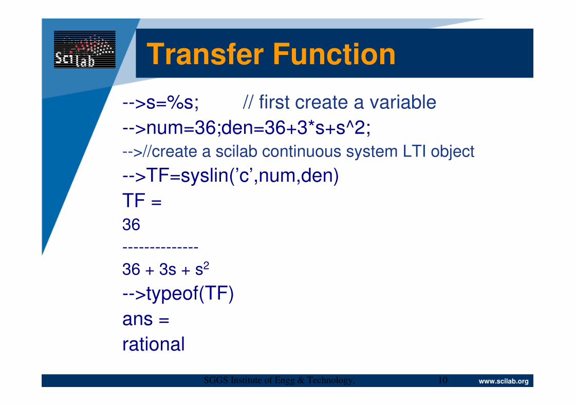
-->s=%s; // first create a variable

-->num=36;den=36+3*s+s^2;-->//create a scilab continuous system LTI object

-->TF=syslin(’c’,num,den)

TF =36

--------------

36 + 3s + s2

-->typeof(TF)

ans =

rational

Company LOGO


4

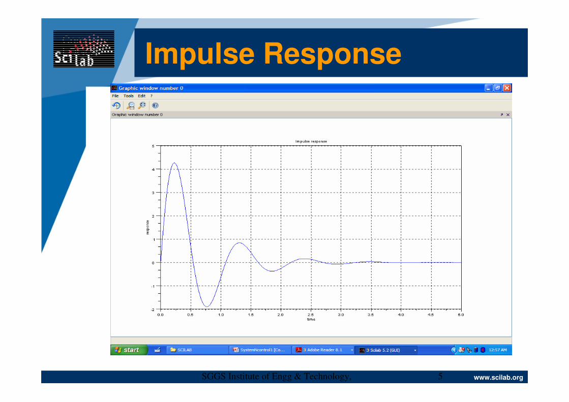
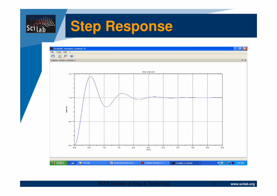
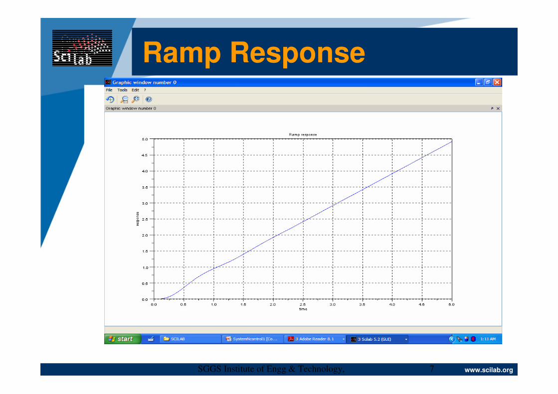
Impulse, Step, and Ramp Response

-->t=linspace(0,5,500);

-->imp_res=csim('imp',t,TF);

-->plot(t,imp_res),xgrid(),xtitle('Impulse response','time','response');

-->step_res=csim('step',t,TF);

-->plot(t,step_res),xgrid(),xtitle('Step response','time','response');

-->ramp_res=csim(t,t,TF);

-->plot(t,ramp_res),xgrid(),xtitle('Ramp response','time','response');

Company LOGO


5

Impulse Response

Company LOGO


6

Step Response

Company LOGO


7

Ramp Response

Company LOGO


8

TF to SS Conversion-->SS1=tf2ss(TF)

SS1 =

SS1(1) (state-space system:)

!lss A B C D X0 dt !

SS1(2) = A matrix =

0. 8.

- 4.5 - 3.

SS1(3) = B matrix =

0.

6.

SS1(4) = C matrix =

0.75 0.

SS1(5) = D matrix =

0.

SS1(6) = X0 (initial state) =

0.

0.

SS1(7) = Time domain = c

Company LOGO


9

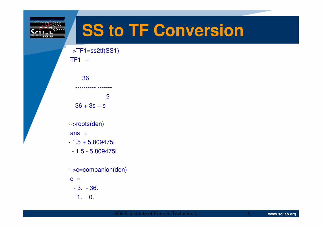
SS to TF Conversion-->TF1=ss2tf(SS1)

TF1 =

36

---------- -------

2

36 + 3s + s

-->roots(den)

ans =

- 1.5 + 5.809475i

- 1.5 - 5.809475i

-->c=companion(den)

c =

- 3. - 36.

1. 0.

Company LOGO


10

Transfer Function

-->s=%s; // first create a variable

-->num=36;den=36+3*s+s^2;-->//create a scilab continuous system LTI object

-->TF=syslin(’c’,num,den)

TF =36

--------------

36 + 3s + s2

-->typeof(TF)

ans =

rational

Company LOGO


11

Transfer Function

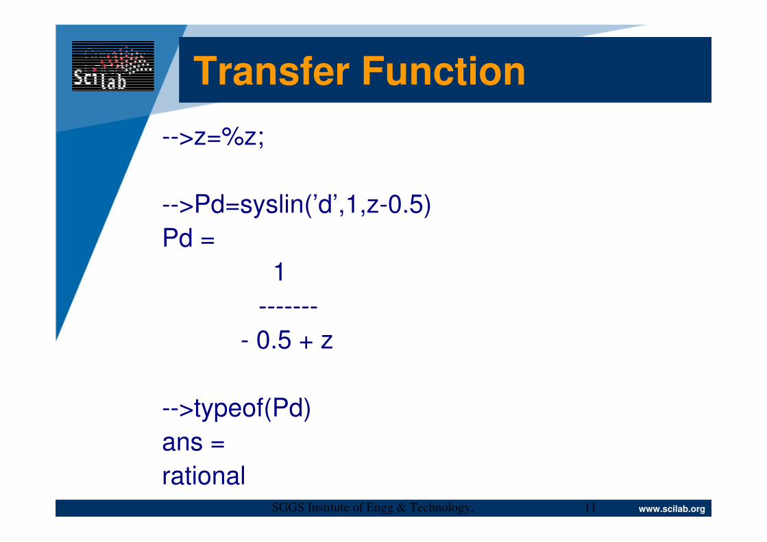
-->z=%z;

-->Pd=syslin(’d’,1,z-0.5)

Pd =

1

-------

- 0.5 + z

-->typeof(Pd)

ans =

rational

Company LOGO


12

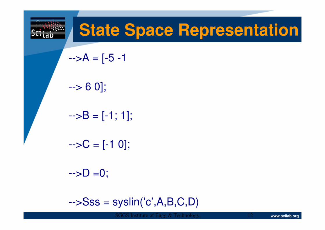
State Space Representation

-->A = [-5 -1

--> 6 0];

-->B = [-1; 1];

-->C = [-1 0];

-->D =0;

-->Sss = syslin(’c’,A,B,C,D)

Company LOGO


13

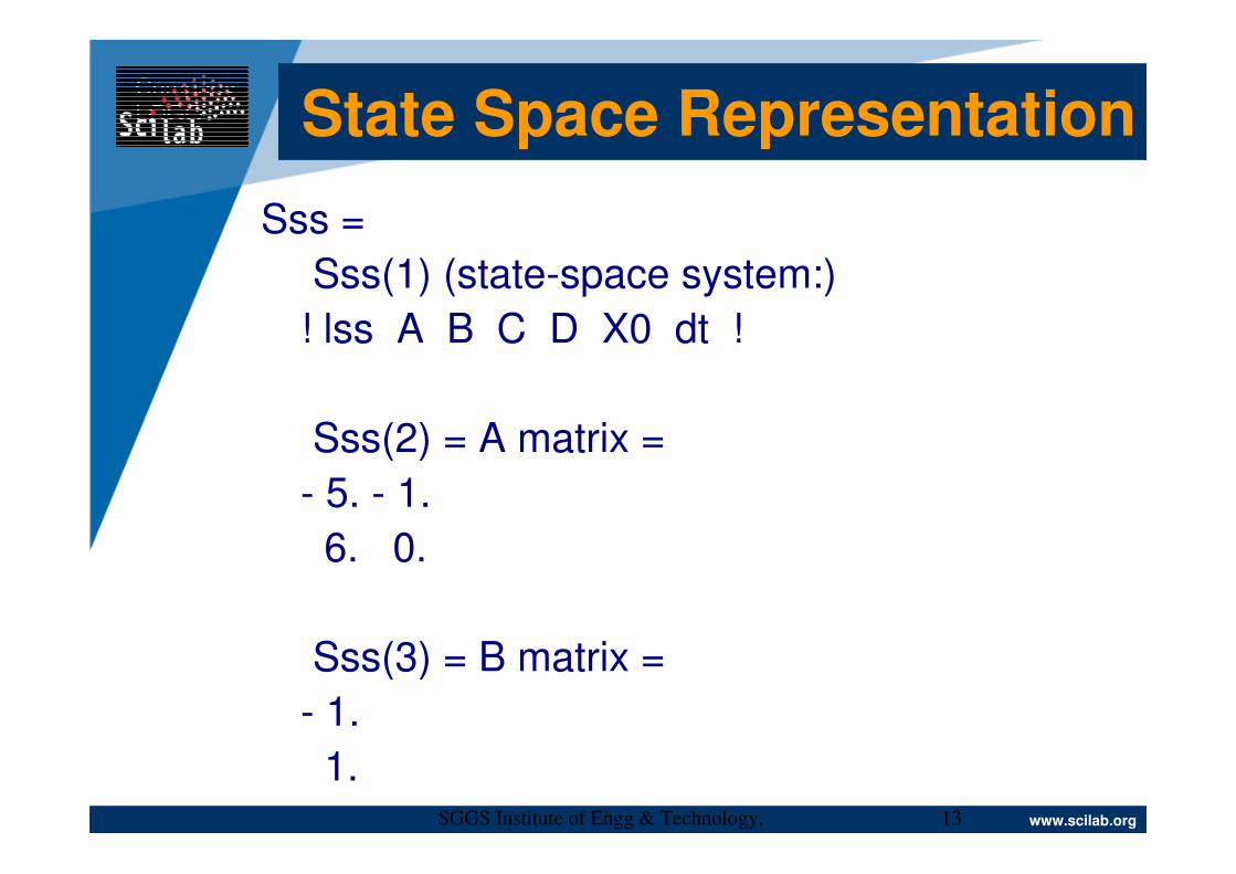
Sss =

Sss(1) (state-space system:)

! lss A B C D X0 dt !

Sss(2) = A matrix =

- 5. - 1.

6. 0.

Sss(3) = B matrix =

- 1.

1.


Company LOGO


14

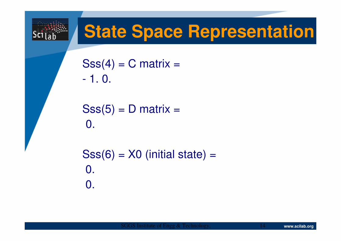
Sss(4) = C matrix =

- 1. 0.

Sss(5) = D matrix =

0.

Sss(6) = X0 (initial state) =

0.

0.


Company LOGO


15

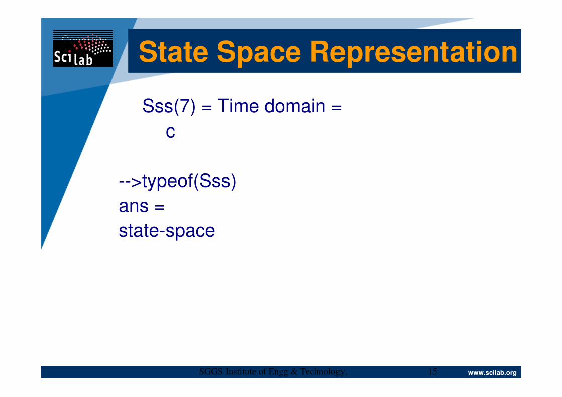
Sss(7) = Time domain =

c

-->typeof(Sss)

ans =

state-space


Company LOGO


16

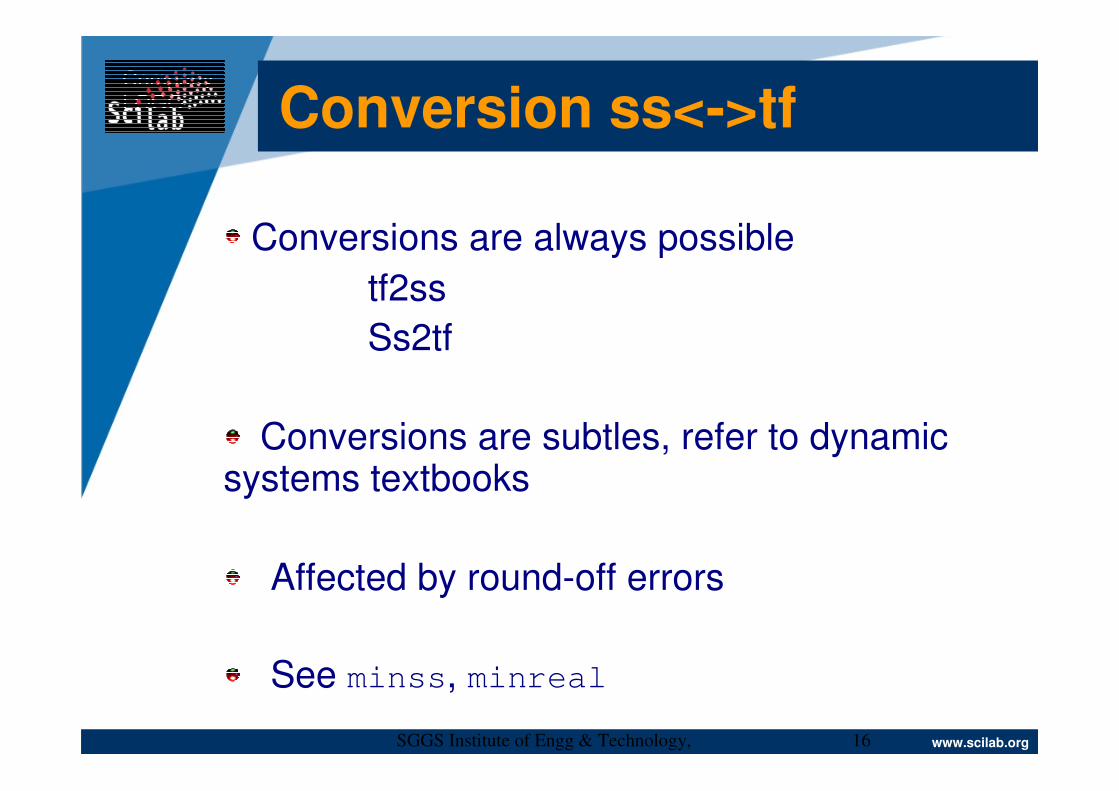
Conversion ss<->tf

Conversions are always possible

tf2ss

Ss2tf

Conversions are subtles, refer to dynamic systems textbooks

Affected by round-off errors

See minss, minreal

Company LOGO


17

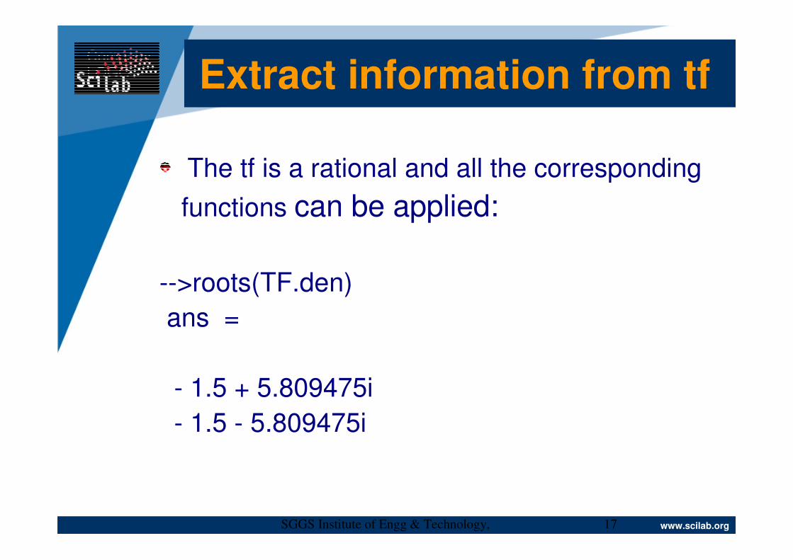
Extract information from tf

The tf is a rational and all the corresponding

functions can be applied:

-->roots(TF.den)

ans =

- 1.5 + 5.809475i

- 1.5 - 5.809475i

Company LOGO


18

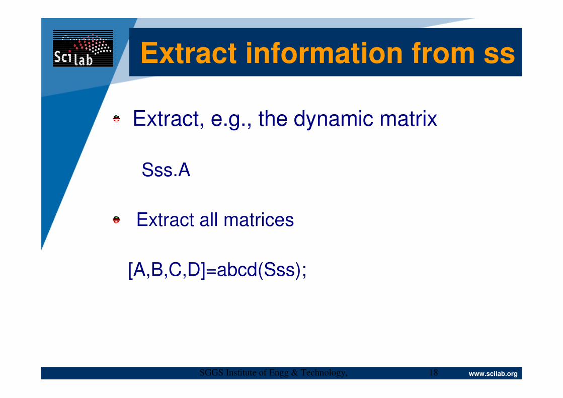
Extract information from ss

Extract, e.g., the dynamic matrix

Sss.A

Extract all matrices

[A,B,C,D]=abcd(Sss);

Company LOGO


19

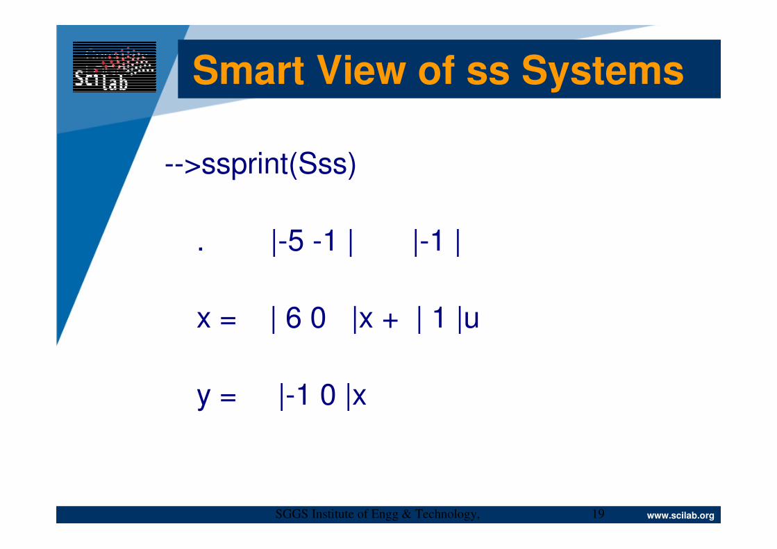
Smart View of ss Systems

-->ssprint(Sss)

. |-5 -1 | |-1 |

x = | 6 0 |x + | 1 |u

y = |-1 0 |x

Company LOGO


20

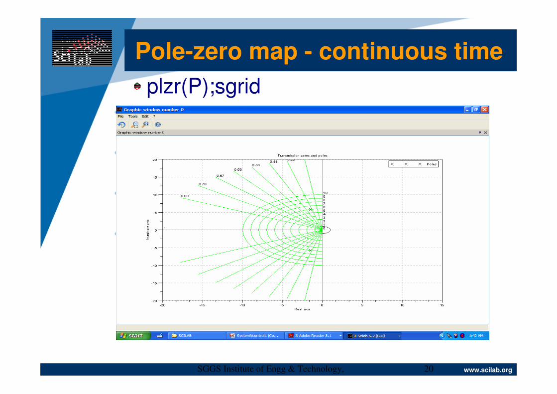
Pole-zero map - continuous time

plzr(P);sgrid

Company LOGO


21

Pole-zero map-discrete time

plzr(P);zgrid

Company LOGO


22

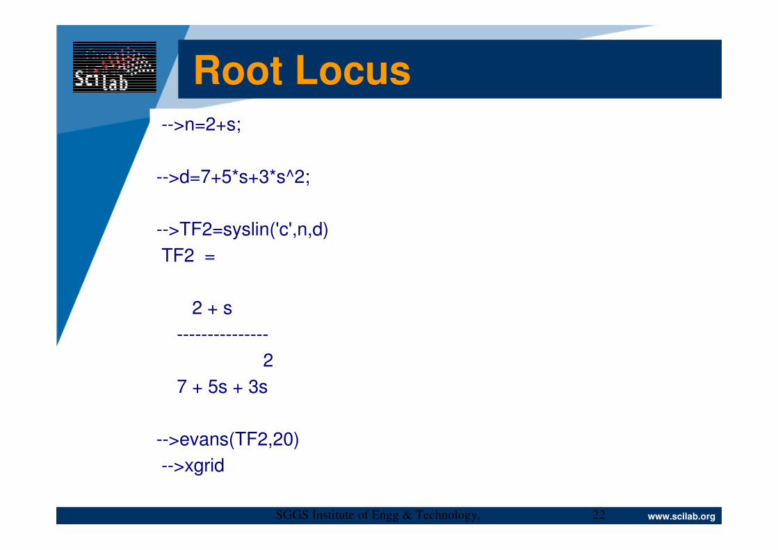
Root Locus-->n=2+s;

-->d=7+5*s+3*s^2;

-->TF2=syslin('c',n,d)

TF2 =

2 + s

---------------

2

7 + 5s + 3s

-->evans(TF2,20)

-->xgrid

Company LOGO


23

Default points useless! use evans(TF2,20)

Root Locus

Company LOGO


24

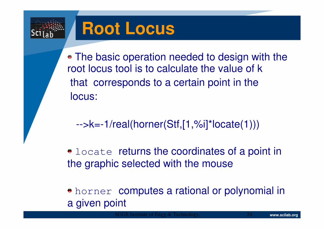
The basic operation needed to design with the root locus tool is to calculate the value of k

that corresponds to a certain point in the

locus:

-->k=-1/real(horner(Stf,[1,%i]*locate(1)))

locate returns the coordinates of a point in the graphic selected with the mouse

horner computes a rational or polynomial in a given point

Root Locus

Company LOGO


25

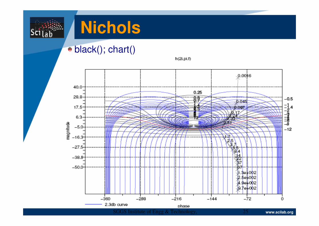
Nicholsblack(); chart()

Company LOGO


26

The curve is parametrized according to a

constant range(!)

Continuous time: [10−3, 103]Hz

Discrete time: [10−3, 0.5]

Better to use the whole syntax assigning

frequency range:

black(sl, [fmin,fmax] [,step] [,comments])

Nichols

Company LOGO


27

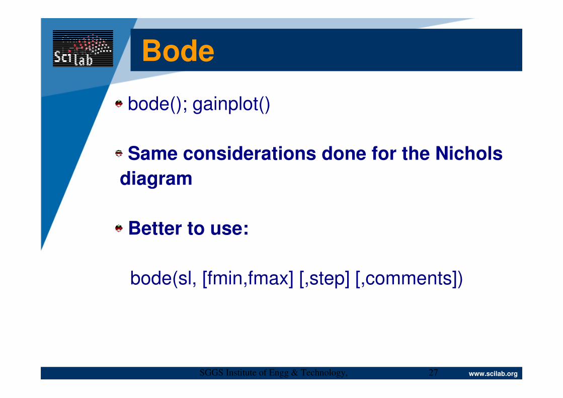
Bode

bode(); gainplot()

Same considerations done for the Nichols

diagram

Better to use:

bode(sl, [fmin,fmax] [,step] [,comments])

Company LOGO


28

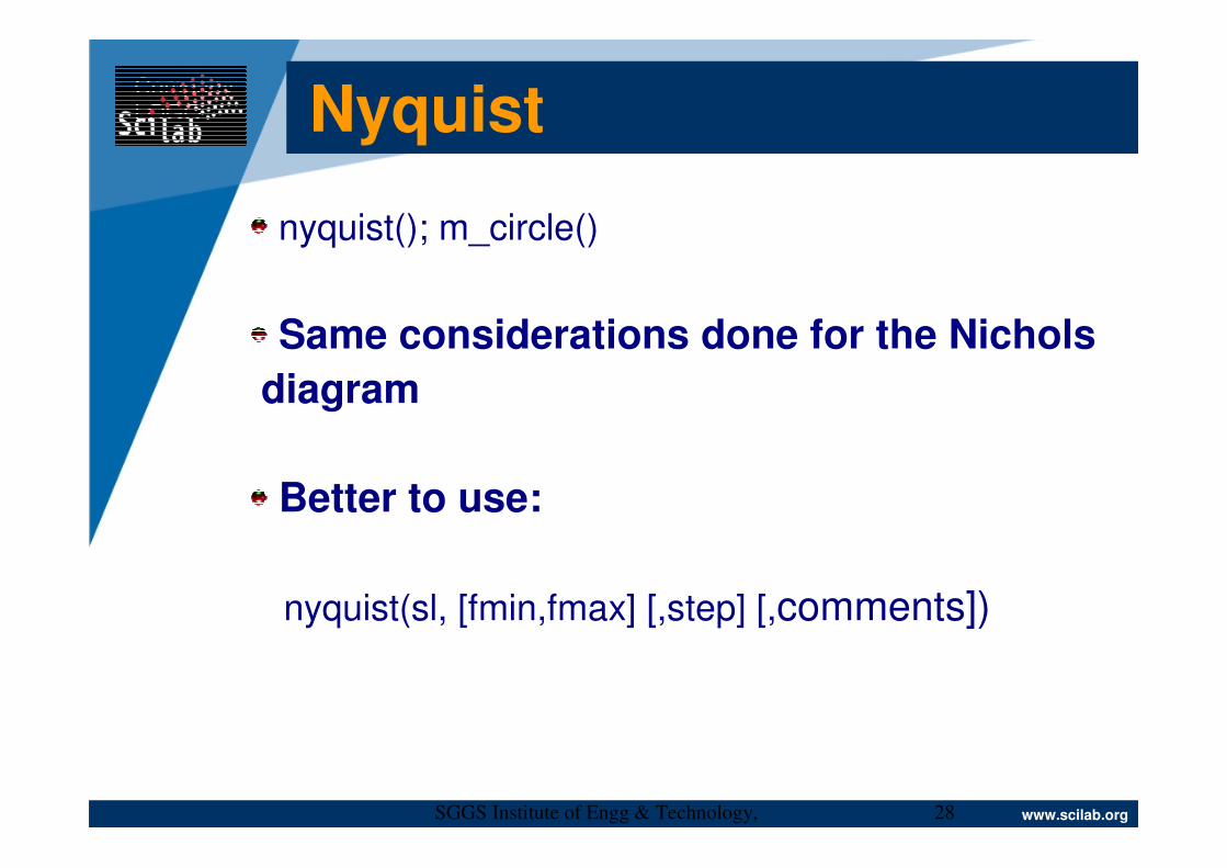
Nyquist

nyquist(); m_circle()

Same considerations done for the Nichols

diagram

Better to use:

nyquist(sl, [fmin,fmax] [,step] [,comments])

Company LOGO


29

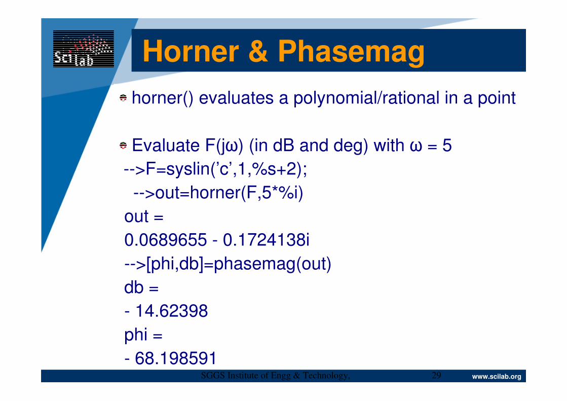
Horner & Phasemag

horner() evaluates a polynomial/rational in a point

Evaluate F(jω) (in dB and deg) with ω = 5

-->F=syslin(’c’,1,%s+2);

-->out=horner(F,5*%i)

out =

0.0689655 - 0.1724138i

-->[phi,db]=phasemag(out)

db =

- 14.62398

phi =

- 68.198591

Company LOGO


30

A Final Bird’s-Eye View

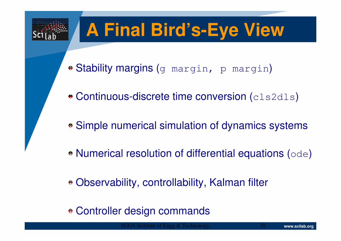
Stability margins (g margin, p margin)

Continuous-discrete time conversion (cls2dls)

Simple numerical simulation of dynamics systems

Numerical resolution of differential equations (ode)

Observability, controllability, Kalman filter

Controller design commands

Company LOGO


31

Thank You !!!

Date post:	02-Jan-2017
Category:	Documents
Upload:	vannga
View:	228 times
Download:	5 times

Scilab in System and Control by Dr. Balasaheb M. Patre, SGGS ...

Documents