Scotland's Rural College

The cost of emission mitigation by legume crops in French agriculture

Dequiedt, B; Moran, D

Published in:Ecological Economics

DOI:10.1016/j.ecolecon.2014.12.006

Print publication: 01/01/2015

Document VersionPeer reviewed version

Link to publication

Citation for pulished version (APA):Dequiedt, B., & Moran, D. (2015). The cost of emission mitigation by legume crops in French agriculture.Ecological Economics, 110, 51 - 60. https://doi.org/10.1016/j.ecolecon.2014.12.006

General rightsCopyright and moral rights for the publications made accessible in the public portal are retained by the authors and/or other copyright ownersand it is a condition of accessing publications that users recognise and abide by the legal requirements associated with these rights.

• Users may download and print one copy of any publication from the public portal for the purpose of private study or research. • You may not further distribute the material or use it for any profit-making activity or commercial gain • You may freely distribute the URL identifying the publication in the public portal ?

Take down policyIf you believe that this document breaches copyright please contact us providing details, and we will remove access to the work immediatelyand investigate your claim.

Download date: 01. Mar. 2020

3

The cost of emissions mitigation by legume crops in French 1

agriculture 2

Benjamin Dequiedta*, Dominic Moranb 3

a Climate Economics Chair, Paris 75002, France, and INRA, Economie Publique, 4

avenue Lucien Brétignières 78850 Thiverval-Grignon, France. 5

b Land Economy and Environment Research Group, Scotland’s Rural College, 6

Edinburgh EH9 3JG, Scotland 7

* Corresponding author. 8

Email Adress : benjamin.dequiedt@chaireeconomieduclimat.org. Phone Number: 9

+33 (0)1 73 01 93 42. 10

11

Abstract 12

13

This paper considers the cost of greenhouse gas mitigation potential of legume crops in 14

French arable systems. We construct marginal abatement cost curves to represent this 15

mitigation or abatement potential for each department of France and provide a spatial 16

representation of its extent. Despite some uncertainty, the measure appears to offer significant 17

low cost mitigation potential. We estimate that the measure could abate half of the emissions 18

reduction sought by a national plan for the reduction of chemical fertilizers emissions by 19

2020. This would be achieved at a loss of farmlands profit of 1,2%. Considering the 20

geographical heterogeneity of cost, we suggest that a policy implementing carbon pricing in 21

agriculture would be more efficient than a uniform regulatory requirement for including the 22

crop in arable systems. 23

24

4

Key words: Agriculture, greenhouse gas mitigation, legumes, cost-effectiveness 25

26

5

27

1 Introduction 28

29

Agriculture accounts for a significant proportion of total greenhouse gas (GHG) emissions 30

both in France and at the European level. In 2011, European Union agriculture accounted for 31

461 million tCO2eq, while in France the amount was 92,5 million tCO2eq (respectively 10,8 32

and 20,6% of European and French GHG emissions including land use, land use change and 33

forestry according to UNFCCC1 National Inventory Report, 2013). A recent European 34

Commission communication (European Commission, 2014) on the policy framework for 35

climate and energy indicated that emissions from sectors outside the EU Emission Trading 36

Scheme (EU-ETS) would need to be cut by 30% below the 2005 level by 2030. At the same 37

time, within the framework of the 'energy-climate' package France has committed to reduce 38

emissions of its sectors not covered by the EU-ETS by 14% by 2020 compared to 2005 39

emissions levels (European Union, 2009). 40

41

Given these ambitions, there is increasing scrutiny of the mitigation measures and specifically 42

their cost relative to other option available within agriculture and in other sectors. This paper 43

considers the abatement of emissions from crop fertilization, which represents a major source 44

of emissions from French agriculture (a fifth of French agricultural emissions2). This 45

comprises emissions of nitrous oxide mainly emitted during the process of denitrification of 46

nitrogenous fertilizers spread on arable land. The paper assesses the overall abatement 47

1 United Nations Framework Convention on Climate Change.

2 Calculated by dividing the 20,29 MtCO2eq emissions from crops (see appendix A) by the 94,3 MtCO2eq

French agricultural emissions (CITEPA, 2012).

6

potential of a key measure, the introduction of leguminous crops, and the associated costs and 48

co-benefits in farm systems. 49

50

Legumes (fabaceae), commonly known in France as alfalfa, pea, or bean family, have the 51

ability to naturally fix atmospheric nitrogen and can reduce N2O emissions compared with 52

conventional crops (maize, wheat, barley, oilseed, rape). This function is conferred by 53

rhizobium bacteria that live in symbiosis at the level of their roots in little organs called 54

nodules. As a consequence, they need far less fertilizer thanks to the fixing effect allowing 55

nitrogen to stay in the ground for up to two years after planting. This contributes additional 56

amounts of nitrogen to subsequent crop in rotations. Studying alternative crop emissions, 57

Jeuffroy et al. (2013) demonstrated that legume crops emit around five to seven times less 58

GHG per unit area compared with other crops. Measuring N2O fluxes from different crops 59

they show that peas emitted 69 kgN2O/ha; far less than winter wheat (368 kgN2O/ha) and 60

rape emissions (534,3 kgN2O/ha). Moreover, compared to the emissions from cattle meat 61

production, human consumption of peas instead of meat leads to 85 to 210 times less N2O 62

emissions for the same content of protein ingested3. Despite this mitigation benefit, N-fixing 63

crops have low agronomic performance (see appendix A) and consequently their introduction 64

in arable systems will, in most regions, incur a penalty in terms of farm revenue. 65

66

Recent research (Pellerin et al. 2013) has suggested the cost of GHG mitigation via grain 67

legumes at around 19 euros/tCO2eq. This paper scrutinises this assessment by proposing three 68

3 20-37 gN2O/kg protein for meat and 0,17-0,23 gN2O/kg protein for peas. The amount of emissions for meat is

obtained using the N2O content from feed fertilization and manure management included in cattle meat from

Dollé et al. (2011) of 3,026 kgCO2eq and 1,615 kgCO2eq per kg of meat. The amount of emissions for pea is

obtained using the yield of 25-34 q/ha from Agreste data..The protein content of meat (27,6g/100g) and peas (8,8

g/100g) required for the calculation are from Ciqual (2012).

7

improvements: (1) determining the spatial variation of cost across French Departments; (2) 69

studying how cost varies according to reduction targets; and (3) analyzing the sensitivity of 70

the abatement cost with respect to agricultural seed prices and farmers’ ability to exploit low 71

abatement cost. 72

73

Here, abatement cost assessment is linked to the substitution of other arable crops by legume 74

crops in farmlands simulating two consecutive years, so as to integrate the fixing effect of the 75

preceding period. This methodology allows the derivation of a marginal abatement cost curve 76

for each French metropolitan geographical area4. The results are then subject to a sensitivity 77

analysis to examine growers’ responses to low cost abatement, crops prices and agricultural 78

input prices. 79

80

The paper is structured as follows. The next section presents the context of N-fixing crops 81

cultivation in France and in Europe and section 3 analyses abatement cost assessment in the 82

scientific literature. Section 4 describes the methodology. Section 5 analyses the results and 83

compares them with the previous INRA (National Institute of Agronomic Research) study 84

(Pellerin et al., 2013). Finally, a discussion considers the policy relevance of carbon pricing to 85

promote N-fixing crops. 86

87

2 Context 88

89

4 Each geographical area corresponds to a department. In the administrative divisions of France, the department

(French: département) is one of the three levels of government below the national level. It is situated between the

region and the commune.

8

Despite their beneficial properties, the area planted to legumes in France has been on a steady 90

downward trend. For fodder legumes the fall started in the 1960’s from a high of 17% of the 91

French arable land. The area then decreased steadily, reaching 2% in 2010 (Duc et al. 2010). 92

For grain legumes, the fall began later at the end of the 1980’s after years of political effort to 93

develop them through the common agricultural policy (CAP) (Cavaillès, 2009). 94

95

This decline is due to several factors. First an increasingly meat-based diet incorporating less 96

vegetable proteins led to lower consumption of legumes by humans. The General Commission 97

for Sustainable Development reports that in France between 1920 and 1985 human seed 98

legume consumption fell from 7,3 kg/person/year to 1,4 kg/person/year (Cavaillès, 2009). 99

This trend coincided with a change in livestock feeding regimes, with legume-based rations 100

being increasingly replaced by maize silage, grass plants and imported soybean meal. The loss 101

of agricultural nitrogen due to this switch in farmlands was compensated by chemical 102

fertilizers, which had become increasingly price-competitive since the 1960’s. 103

Simultaneously, trade agreements on the abolition of customs tariffs between Europe and the 104

United States favored American soybean imports. Finally, a lack of agronomic research 105

dedicated to legumes compared with common crops, led to a relative decrease of their 106

agronomic performance (Cavaillès, 2009). 107

108

In France, as in the rest of the European Union (EU) these factors have led to a strong 109

dependency on soya imported from America to feed livestock. In 2009, soya was the largest 110

food commodity imported into the EU (12,5 million tons) ahead of palm oil and bananas 111

(FAO5). These imports come mainly from South America (49% from Brazil and 31% from 112

Argentina (European Commission, 2011)), and at a significant cost : the average annual trade 113

5 http://faostat.fao.org/

9

balance, calculated over the period 2004-2008, represented a loss equivalent to 1 billion euros 114

(Cavaillès, 2009) for France and up to 10,9 billion euros for the EU. It follows that increasing 115

legume areas in French agriculture can both mitigate GHG emissions and limit dependency on 116

feed imports. This is all the more so given the trend of increasing chemical fertilizer prices. In 117

2010, the price of fertilizers and soil conditioners spread on farmland in France were some 118

65% higher than 1990; this increase being largely related to higher global energy prices. Thus, 119

the increasing scarcity of fossil fuels provides another reason to explore the potential 120

development of legume crops. 121

122

3 Cost-effectiveness analysis in the literature 123

124

For cost-effectiveness analysis Vermont and De Cara (2010) identify three broad approaches 125

for the derivation of marginal abatement cost curves (MACCs), the device typically used to 126

evaluate pollution abatement costs and benefits. These are: i) a bottom-up or engineering 127

approach; ii) an economic approach consisting of modeling the economic optimization of a set 128

of (in this case) farm operations; iii) a partial or general equilibrium approach that extends and 129

relaxes some of the assumptions about wider price effects induced by mitigation activity. 130

131

The engineering approach focuses on the potential emission reduction of individual measures 132

and observes their cumulated abatement and associated costs. The required data to appraise 133

abatement costs are ideally collected from measures applied on test farms, thereby reducing 134

some uncertainty the estimated cost and mitigation potential for each mitigation measure. It is 135

normally the case that more measures are assessed using the engineering approach relative to 136

the economic approach (MacLeod et al. 2010, Moran et al. 2010, Pellerin et al. 2013). 137

138

10

The economic approach consists of modeling the economic optimization of a set of farm 139

operations located within a given geographical scale. The objective function is typically to 140

maximize profit of these farms under given constraints such as available arable land or even 141

lay fallow land as imposed by agricultural policies. The introduction of a carbon tax as a new 142

constraint, allows the model to reconfigure farm activities to accommodate the necessary 143

GHG emissions reductions. The resulting loss in profit (opportunity cost) and GHG reduction 144

provide the relevant abatement cost information. 145

146

Equilibrium models relax some of the cost assumptions made in the economic approach and 147

include a description of the demand for agricultural products thereby allowing a price 148

feedback into the cost of mitigation (Vermont and De Cara, 2014). Their level of spatial 149

disaggregation is generally lower than that of bottom-up models and their geographic scope 150

and coverage are generally wider. This approach has been used to assess abatement cost at the 151

level of the USA (Schneider and McCarl, 2006; Schneider et al., 2007; McCarl and 152

Schneider, 2001). 153

154

A noteworthy difference between the approaches is the frequent observation of negative cost 155

options in the engineer approach for some options (Moran et al., 2010; MacKinsey & 156

Company, 2009). These are obviated in any optimization approach and are in any case 157

questioned by some authors. Kesicki and Ekins (2012) for example suggest that they more 158

likely imply a failure to assess some hidden costs (diffusion of the information, administration 159

barriers) than any real opportunity to reduce emissions while increasing farm gross margins. 160

Another observation is that each mitigation measure in the engineering approach is associated 161

with a constant marginal cost – creating a stepwise marginal abatement curve (each step 162

corresponding to an option). This observation suggests that the economic potential per ton 163

11

CO2 equivalent mitigation is the same for each specific option irrespective of spatial scale or 164

in terms of the overall volume of emission reduction, which would seem unlikely. Indeed, due 165

to regional variability in soils, farm systems, climate and yields, abatement cost would also 166

vary for any individual mitigation measure. 167

168

Results from studies employing the economic approach are depicted by continuous increasing 169

abatement cost curves, with no negative cost. An advantage of these studies is optimization of 170

fewer mitigation measures over a large number of farm types. For example De Cara and Jayet 171

(2011) modeled around 1300 EU farms optimizing animal feed, a reduction in livestock 172

numbers, a reduction of fertilization and the conversion of croplands to grasslands or forests. 173

174

Legumes have been specifically assessed in a UK study constructing a national MACC for 175

agricultural GHG emissions (Moran et al., 2010). The marginal abatement cost obtained for 176

legume crops appears constant and very high (14280 £/tCO2eq equivalent to 17000 177

euros/tCO2eq). This is in stark contrast to Pellerin et al. (2013) estimate of only 19 euros/t 178

CO2eq. To explore some of the reasons for this disparity we adopt a predominantly 179

engineering approach combined with elements of an economic approach to explore the role of 180

farm systems decision-making around the adoption of legumes as a specific measure that can 181

influence farm profitability. 182

183

4 Method 184

185

4.1 Defining emissions and gross margin 186

The analysis assesses the abatement potential in 96 French metropolitan geographical areas, 187

each considered as a single farm decision unit. The analysis is confined to the within farm 188

12

gate effects and does not account for the upstream or downstream impacts; e.g. associated 189

with lower fertilizer production, or the emission mitigation benefit related to enteric 190

fermentation of cattle consuming legumes (McCaughey et al., 1999). In each geographical 191

area, farmland emissions and profits are calculated and decomposed for each crop (Common 192

Wheat, Durum Wheat, Barley, Maize, Sunflower, Rapeseed, Pea, Horse bean and Alfalfa). 193

We followed the 2006 IPCC Guidelines for National Greenhouse Gas Inventories (IPCC, 194

2006) to estimate N2O emissions per hectare. Using mineral nitrogen spreading rates and 195

organic spreading rates from the Agricultural Practices survey (Agreste, 2010) we calculate 196

the following kinds of emission sources: 197

- direct emissions, happening directly on the field, 198

- indirect emissions, covering emissions from atmospheric redeposition and leaching 199

and runoff, 200

- emissions from crop residues. 201

The formula that determines each crop gross margin in each geographical area is summarized 202

as follows (Ecophyto R&D, 2009) : 203

𝐺𝑀𝑘,𝑖 = (𝑝𝑟𝑖𝑐𝑒𝑘,𝑖 × 𝑦𝑖𝑒𝑙𝑑𝑘,𝑖 ) − (𝑒𝑥𝑝𝑝ℎ𝑦𝑡𝑜,𝑘,𝑖 + 𝑒𝑥𝑝𝑓𝑒𝑟𝑡𝑖,𝑘,𝑖 + 𝑒𝑥𝑝𝑠𝑒𝑒𝑑,𝑘,𝑖 )

204

Where GM k,i is the gross margin calculation for each crop i in each geographical area k (in 205

euro per ha). Price k,i is the crop price in euros per ton and yield k,i is expressed in tons per 206

hectare. The expenses in phytosanytary products (expphyto,k,i ), in fertilizers spread (expferti,k,i ) 207

and in seed (expseed,k,i) are all measured in euros per hectare. 208

4.2. Baseline 209

13

Appendix A shows the results for the main crops cultivated in France and gives the baseline 210

for overall farmland gross margin (6,4 billion euros) and for emissions (20,4 MtCO2eq). 211

When comparing these emissions with those of the national inventory report, we observe that 212

the amount represents less than half of the category ‘Agricultural Soils’ (46,7 MtCO2eq 213

(CITEPA, 2012)). This category represents all N2O emissions linked to soil fertilization both 214

from cropland and grassland soils. Hence the baseline emissions assessed here is quite 215

coherent since we only focus here on emissions from croplands which represent less than half 216

of the French Utilized Land Area6. 217

4.3. Introduction of legumes onto croplands 218

Legume crops have low emissions per hectare and a low gross margin compared with other 219

crops. Consequently, in most geographical areas, as the overall utilized land area remains 220

constant, increasing the share of in N-fixing crops induces a reduction of both profit and 221

emissions. 222

Additional legume crop areas are introduced in each geographical area by 10% increments to 223

the initial legumes area. The loss of profit (dCost) divided by the reduction of emission 224

(dEmissions) linked to these additional areas represents the marginal abatement cost. The 225

marginal cost and marginal emissions also integrate the preceding fixing effect, which induces 226

higher gross margin and lower emission for following year crops that have been preceded by 227

legumes. 228

𝑀𝑎𝑟𝑔𝑖𝑛𝑎𝑙 𝐴𝑏𝑎𝑡𝑒𝑚𝑒𝑛𝑡 𝐶𝑜𝑠𝑡 = 𝑑𝐶𝑜𝑠𝑡

𝑑𝐸𝑚𝑖𝑠𝑠𝑖𝑜𝑛𝑠

6 According to Agreste, the Utilized Land Area represents 28 million hectare in France. In appendix A, we

observe that cropland area covers less than half of this area: 13,6 million hectares.

14

Legume substitution continues until a marginal abatement cost of 125 euros/tCO2eq has been 229

exceeded per geographical area. This upper abatement cost threshold has been arbitrarily 230

chosen, considering the relative abatement cost in other sectors (Vermont and De Cara, 231

2014)7. 232

In seeking the lowest abatement cost in terms of foregone gross margin per unit emissions, we 233

assume that legume crops displace conventional (non N fixing) crops according to a schedule 234

of progressively increasing gross margin. Thus areas yielding lowest gross margin are 235

converted first. But to avoid complete displacement of conventional crops, a cap is placed on 236

the extent of this displacement. The logic here is that it is difficult to foresee that farmers 237

would be entirely motivated by an abatement cost goal to cultivate legumes to the exclusion 238

of other crops. In reality most farmers would seek to minimize risk by maintaining a level of 239

diversity on their land, which often means that they maintain less profitable crops. For 240

instance, on livestock farms, some less profitable crops are used for feed. In other cases a lack 241

of training and information can also retard the adoption of new practices such as legumes. We 242

consider scenarios in which the limit, termed the variable limit, is assumed to take alternative 243

values of 10%, 30%, 90% and 100%. When the variable limit is 100%, farmers can 244

potentially replace all the crop area, meaning that they are looking for a complete 245

minimization of abatement cost and are strongly sensitive to economic signals for mitigation. 246

On the other hand, a 10% limit means that farmers cannot replace more than 10% of the least 247

profitable crops area. Moreover, we account for the fact that the variable limit is the same for 248

every crop in every geographical area. Allowing for agronomic differences, different national 249

abatement cost curves are therefore presented for the different variable limits: from the 10% 250

7 Vermont and De Cara, 2014 assesses for instance a marginal abatement cost curve for European farms until a

maximum level of 100 euros/tCO2eq

15

scenario corresponding to a low exploitation of minimal abatement cost to a complete use of 251

low abatement cost in the 100% scenario. 252

As legume crops are introduced onto farmland the cumulated cost corresponds to the sum 253

of dCost and the cumulated abatement corresponds to the sum of dEmissions generated at 254

each additional area introduction. These cumulated cost and abatement are obtained both at 255

the regional and national levels. The average mitigation cost is the ratio between cumulated 256

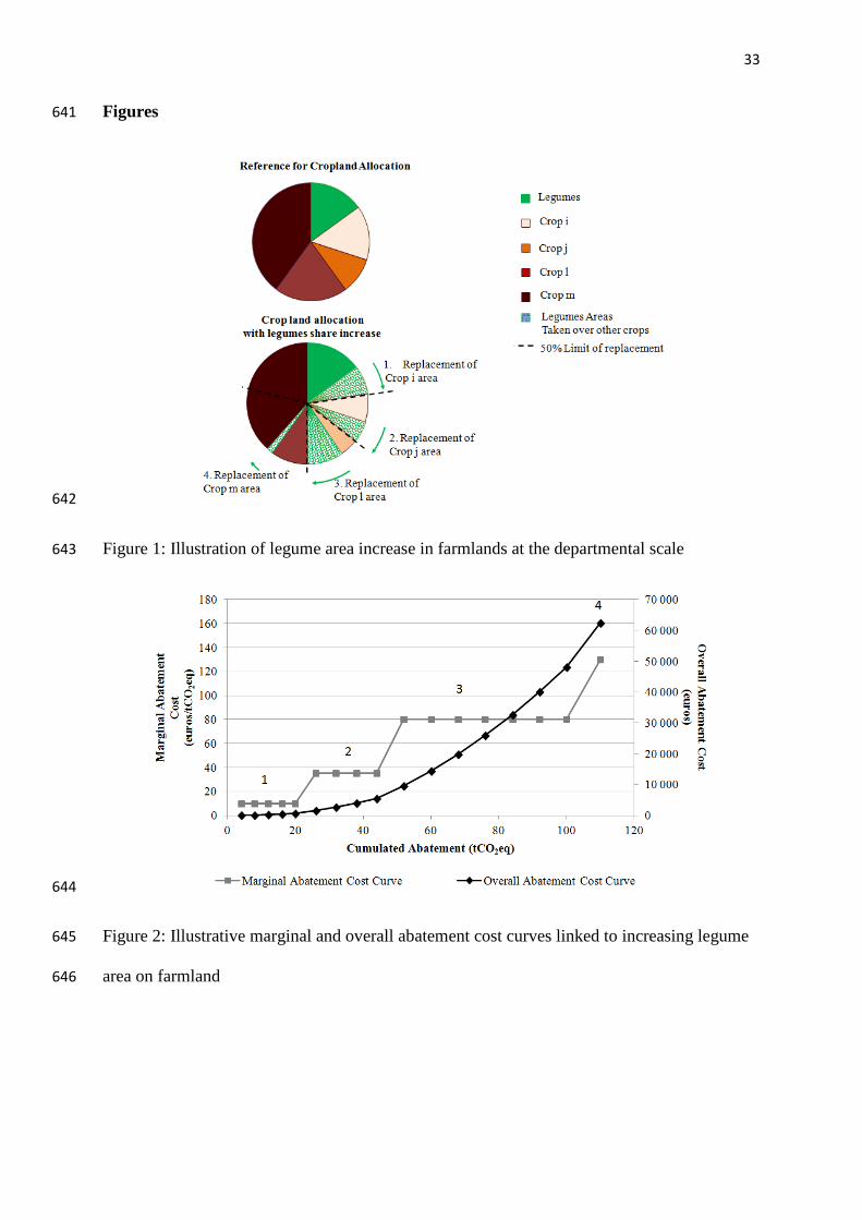
cost and cumulated abatement. Figure 1 illustrates a sample geographical area in which 257

legumes area is increased with a 50% limit. Agricultural land is allocated with only 5 crops, 258

each characterized by a specific emissions rate per hectare and gross margin. Assume the rank 259

of crops considering their ratios of gross margin per emissions is : crop i, crop j, crop l and 260

crop m. Thus, the additional area of legumes first replaces crops i. Once crop i has lost 50% of 261

its area, legumes replace crop j, and so on until the introduction reaches crop m. At this stage, 262

the 125 euros/tCO2eq is achieved, which consequently stops further legume introduction. 263

[Figure 1] 264

The marginal abatement cost of successive areas increments is depicted in figure 2. Each 265

point of the curve corresponds to an additional increase in legume area. For a given crop, the 266

marginal abatement cost is the same whatever the replaced area, which explains the different 267

steps of the curve. The values comprising the overall abatement cost curve is derived from the 268

integral of the marginal abatement cost curve. 269

[Figure 2] 270

5 Results 271

5.1 Abatement potentials and cost 272

273

16

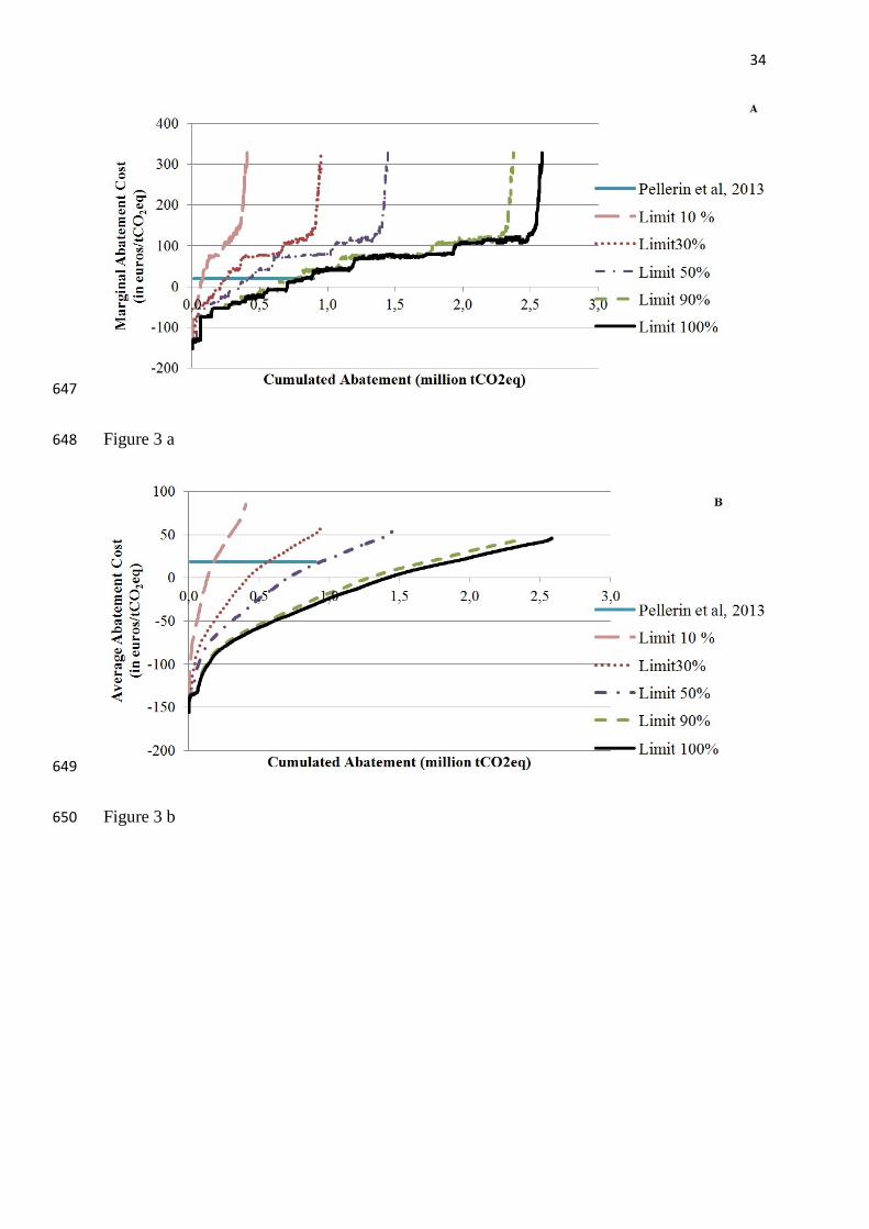
At the national level and assuming the variable limit of 100%, the maximum technical 274

abatement of 2,5 million tCO2eq/year is possible for an overall cost of 118 million euros/year 275

(see figure 3. c). This corresponds to an increase of 1,6 Mha of legumes and an average 276

abatement cost of 43 euros/tCO2eq. 277

278

The overall cost depends on the volume of emissions reduction. Since displaced crops in each 279

geographical area are ordered by their ratio of gross margin per emission, the lower the 280

abatement targets the lower the overall cost. For example, if the target of emission reduction 281

is reduced by 30%, to 1,7 MtCO2eq, the average abatement cost is reduced by 80% to 14 282

euros/tCO2eq. If the target is lower than 1,4 MtCO2eq, we find a negative abatement cost, 283

implying that legumes are actually now more profitable than the crop that is displaced . 284

285

Reducing the variable limit also reduces the overall abatement potential while increasing the 286

abatement cost. Fixing the limit to either 10% or 90% induces a reduction in the maximum 287

abatement potential of 84% and 8% respectively. We thus observe that results are highly 288

sensitive to this variable. But even if the variable is low, we still observe opportunities to 289

reduce emissions while increasing farm gross margins (see figure 3). 290

291

Pellerin et al. (2013) suggests that legume introduction could provide an overall abatement 292

potential of 0,9 MtCO2eq, at a cost of 17 million euros. This implies an average mitigation 293

cost of 19 euros/tCO2eq. That study did not consider how cost varies with area and hence the 294

potential for negative costs. By illustrating those results (the blue curve in Figures 3b and 3c) 295

alongside those derived in this study, it is possible to see that defining a variable limit of 50%, 296

which is the average scenario, and the most realistic, for the same amount of emission abated, 297

17

we obtain the same overall cost and the same average abatement cost (reached for a marginal 298

abatement cost of 80 euros/tCO2eq). 299

300

[Figure 3 a] 301

[Figure 3 b] 302

[Figure 3 c] 303

304

5.2 Heterogeneity of abatement cost between French geographical areas 305

306

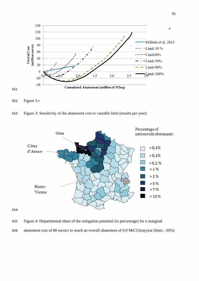
The spatial allocation of the abatement potential between different geographical areas can be 307

represented for the same marginal abatement cost. Figure 4 shows the departmental shares for 308

the same marginal carbon reduction cost threshold (80 euros/tCO2eq) and a 50% limit to 309

achieve the same reduction estimated by Pellerin et al. (2013). The results show considerable 310

geographical variability, with some accounting for a small amount of the 0,9 MtCO2eq 311

national abatement. These geographical areas are mainly located in the south and eastern parts 312

of France, and represent each less than 1% of these overall reduced emissions. Departments 313

with the highest potential are located in the north-west, where the majority of the geographical 314

areas represent each more than 1% of the national abatement. Note that two regions, Orne and 315

Manche, can each contribute more than 10% of the national abatement. 316

317

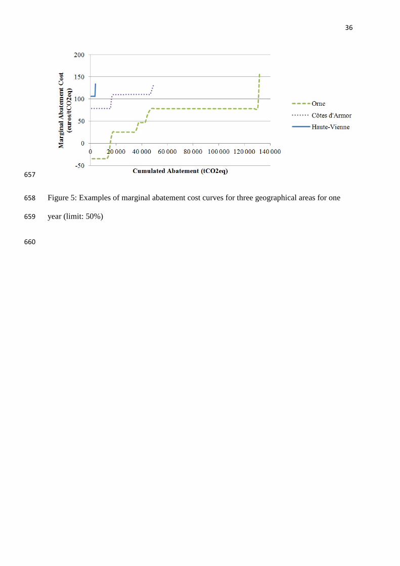
An alternative representation of the cost heterogeneity is presented in figure 5 for three 318

geographical areas: Orne, Haute-Vienne and Côtes d’Armor. Introducing legumes in Orne is 319

more profitable than in Haute-Vienne or in Côtes d’Armor. In the latter two regions, even for 320

low levels of mitigation the marginal abatement cost is high (respectively 80 euros/tCO2eq 321

and 110 euros/tCO2eq). This cost heterogeneity demonstrates the challenge of setting a 322

18

uniform nationwide target. If, for example the objective of reducing 50 000 tCO2eq GHG 323

emissions were assigned for the three previously mentioned geographical areas, the overall 324

cost would be high relative to the case of one region (Orne), mitigating 130 000 tCO2eq on its 325

own. As a result, this simulation demonstrates the advantages of policy instruments that 326

account for the cost heterogeneity between regions. 327

[Figure 4] 328

[Figure 5] 329

5.3 Sensitivity analysis 330

331

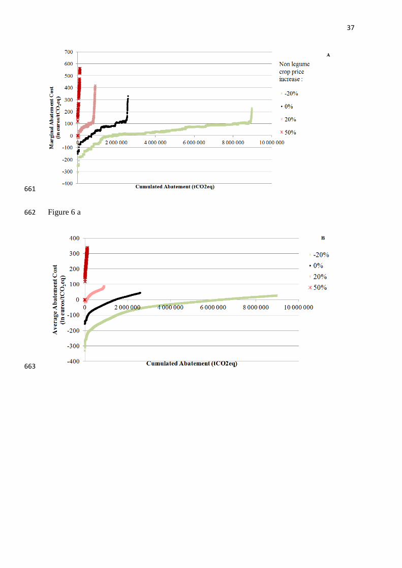
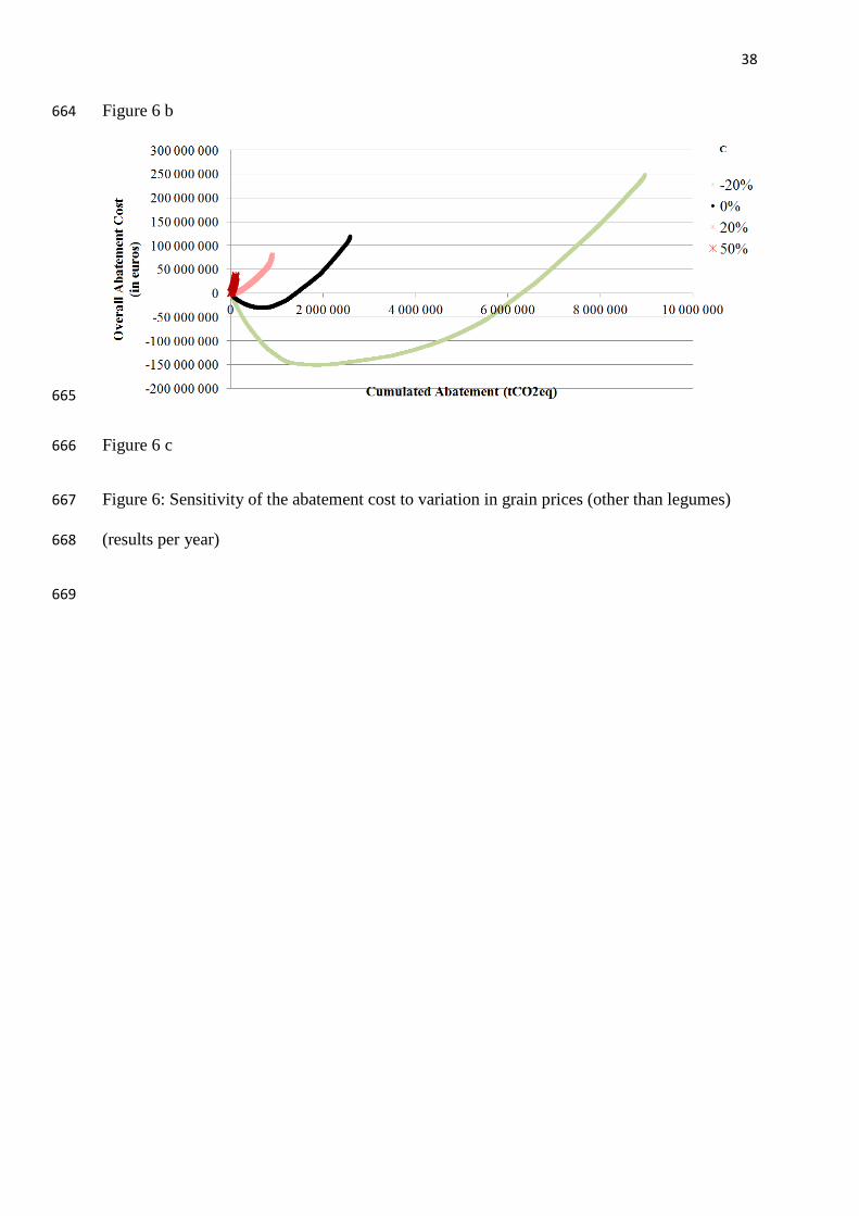
Figure 6 shows the impact on the abatement cost of price variations of conventional crops. 332

When seed prices of alternative crops increase, the opportunity cost of legume introduction 333

rises. On the contrary, when seed prices decrease, the difference of gross margin between 334

legumes and conventional crops decreases as well and makes their introduction less costly. 335

We represent the abatement curves for the follow price increases: -20%, +20% and +50%. For 336

a price decrease of -20%, negative abatement costs appear until an abatement level of 6 337

MtCO2eq. For a price increase of 20%, the opportunity of decreasing emissions while 338

increasing profit disappears completely. The abatement cost becomes considerably high when 339

the increase is 50%. Consequently, we observe a strong sensitivity of abatement cost to the 340

price of conventional crops. 341

342

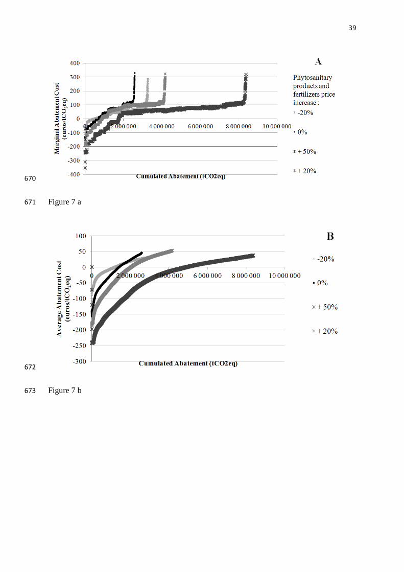
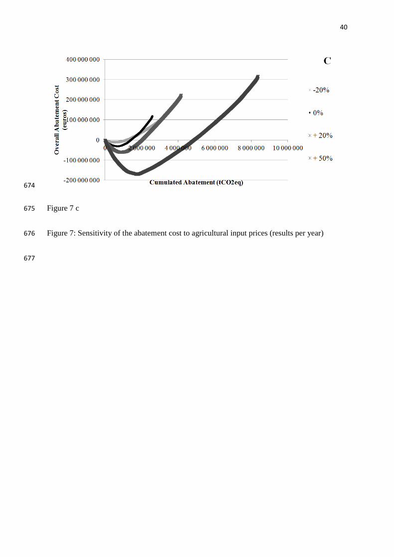
Abatement costs are also highly sensitive to agricultural input prices (fertilizers, seeds and 343

phytosanitary products) (figure 7). A rise of 20% of input prices compared to baseline values 344

determined in the Ecophyto R&D (2009) favors legume introduction by lowering the 345

abatement cost. A higher increase of 50% for a marginal abatement cost of 30 euros/tCO2eq 346

increases the abatement from 0,8 to 2 million tons CO2 equivalent. On markets, input prices 347

19

are not so volatile. Although they rose sharply in 2008-2009, this spike was exceptional 348

relative to recent trends showing more stable increases. The prospect of rising fossil fuel 349

prices, which are inputs to phytosanitary products manufacturing, suggests that the 350

opportunity cost of legumes may be lower in the future. 351

[Figure 6 a] 352

[Figure 6 b] 353

[Figure 6 c] 354

[Figure 7 a] 355

[Figure 7 b] 356

[Figure 7 c] 357

358

6. Discussion 359

360

A problematic observation in the analysis is the presence of negative abatement costs, which 361

raises questions about their veracity. Specifically, it is unclear why farmers would not 362

automatically adopt such profitable measures (and provide associated mitigation) unless it is 363

the case that there are other unaccounted for costs driving decision-making, which are not 364

captured in this analysis. These hidden costs can be attributed to a variety of barriers within 365

and beyond the farm. Some barriers are intrinsic to individual behaviors and imply internal 366

factors (cognition and habit) and social factors (norms and roles) (Moran et al. 2013). 367

Moreover, farmers may be exhibiting risk aversion behavior in response to legume yield 368

variation. In this study, the average legume gross margin is relatively high in some regions, 369

making the crop in rotations more profitable than some of the conventional crops. However, 370

the annual yield of legume disguises significant annual variation that is not represented here. 371

Consequently some farmers, actually grow crops with a lower gross margin to be sure that the 372

20

yield of the crop will be high enough and to avoid any risk of significant loss associated to 373

legumes. This risk aversion is also linked to the volatility of other crop prices, which has a 374

strong impact on abatement cost as shown in figure 5. Furthermore, as noted by Gouldson 375

(2008), some factors are external to the farm. These include a necessity to adapt the 376

organization of agricultural cooperatives to collect the output of legumes. For instance, 377

legumes need adapted silos that are not currently established in all regions in France. The role 378

of cooperatives is also important in the diffusion of information, training and advice in the 379

agricultural sector (Meynard et al., 2013). 380

381

Beyond the apparent paradox of non adoption of negative cost measures, a broader challenge 382

relates to the available policy options available for agricultural mitigation. The CAP reform 383

framework for the 2014-2020 period elevates emissions mitigation as a significant challenges 384

for agriculture (European Commission, 2014). But ongoing debate about the reform is notable 385

for the limited scope of explicit GHG mitigation objectives that are nevertheless being 386

analyzed at national level in several countries (e.g. UK, Ireland, and Netherlands). In France, 387

the Court of Auditors has indicated that climate policy should not only focus on the energy 388

and industry sectors through the EU-ETS, but also on sectors with small and diffuse 389

emissions sources, in particular agriculture (Cour des Comptes, 2014). A similar situation can 390

be observed in the UK, where abatement cost analysis has helped to define an economic 391

abatement potential that is initially being targeted through voluntary agreement with the 392

agricultural sector (AHDB, 2011). The point now at issue is the relevant policy instrument to 393

motivate these emissions reductions at least cost. 394

395

The fact that abatement costs vary strongly from one geographical area to another suggests 396

that these instruments should rely more on market-based approaches, rather than a regulatory 397

21

approach aimed at increasing legumes area directly. Such approaches (e.g. a tax or forms of 398

emissions permits) offer the flexibility of response, thereby increasing the likelihood of 399

realizing the abatement potential identified by marginal abatement cost curves. Specifically, 400

when a carbon price is implemented in a specific sector, agents should reduce their emission 401

until the marginal abatement cost reaches the carbon price (de Perthuis et al., 2010). 402

403

In the case of domestic projects, a carbon price can compensate the costs due to the 404

introduction of additional legume area. In this way, agents will continue to reduce their 405

emissions as long as marginal abatement costs are lower than the benefit of the carbon 406

annuity. Thus, legumes areas rise while minimizing overall abatement cost; in contrast to a 407

blanket regulatory requirement that specifies the area to be planted. 408

409

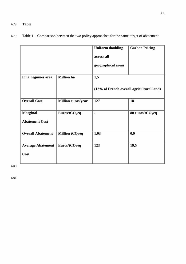
For illustration, we compare the two approaches for the same target for increasing legumes 410

(doubling the current area at national level). This target is chosen since it corresponds to an 411

area that should be cultivated in France to reduce dependence on soya imports (Cavaillès, 412

2009). In the carbon pricing approach, a doubling of legumes at national level happens at a 413

carbon price of 80 euros/tCO2eq. In the uniform regulatory approach, each geographical area 414

is required to double its legumes area. On the face of it, the latter approach appears logical if 415

we consider that each region increases area in proportion of the initial area. Yet, we observe 416

in table 1 that for the same target, the overall abatement cost is far lower under a carbon price 417

(18 million euros) than under a uniform target (127 million euros). 418

419

An experimental initiative with offset payments for legume cultivation is currently being 420

piloted on a voluntary basis by some regional cooperatives (InVivo, 2011). Farmers willing to 421

increase the share of legumes on their land receive a carbon annuity, determined by the level 422

22

of carbon price on the EU ETS8. However, few cooperatives have been part of this initiative. 423

Indeed, the carbon price being relatively low at 5 euros/tCO2eq (CDC Climat, 2014) the offer 424

is not attractive for farmers. An advantage of the MACC analysis presented here is to assess 425

the impact on abatement if this initiative were to become more widespread, subsequently to 426

higher carbon price level. 427

[Table 1] 428

7. Conclusion 429

430

Combining both economic and engineering approaches to the development of abatement cost 431

curves, this study offers a national assessment of the cost-effectiveness of GHG mitigation 432

using legumes in arable systems. This intermediate MACC approach allows for the possibility 433

of negative abatement costs that are typically excluded in economic approaches to MACC 434

construction. It also reveals more granularity in cost information that is usually disguised in 435

the average cost assumptions made in engineering approaches. This is particularly 436

advantageous for illustrating uncertainties linked to agricultural price variation (agricultural 437

input and seed prices volatility) and some hypotheses about the reaction of farmers to 438

economic signals. Finally the approach is useful to display regional variability in costs and 439

hence to illuminate the efficiently of policy alternatives for the introduction of the measure. 440

441

In a realistic scenario, legumes could abate a maximum 7% of chemical fertilizer emissions at 442

a cost of 77 million euros corresponding to a loss of 1,2% of overall profit in France. Win-win 443

abatement could be 3% of chemical fertilizer emissions. Hence, although showing that this 444

8 This project is led under the framework of the Joint Implementation

(http://unfccc.int/kyoto_protocol/mechanisms/joint_implementation/items/1674.php). An assessment report of

the project is drawn up at the moment and should be delivered in the period of January-February 2015.

23

mitigation option could offer low abatement cost, N-fixing crop would need to be combined 445

with other measures to tackle the 14% emissions reduction target of diffuse emissions sectors 446

by 2020 (European Union, 2009). To increase adoption the suggested option of carbon pricing 447

would appear to be more economically efficient than a policy focusing on increasing areas in 448

each geographical area directly. 449

450

An interesting addition to this work would be to investigate the upstream and downstream 451

impact of legume on greenhouse gases and their consequences on abatement cost. The 452

production of chemical fertilizers is responsible for significant CO2 emissions in industries. 453

Hence, the associated decrease of emissions due to chemical fertilizers substitution should 454

decrease abatement cost. Further, the displacement of imported soybean by fodder legumes 455

such as alfalfa would have a positive impact on enteric fermentation, responsible for methane 456

emissions in livestock feeding regimes (Martin et al., 2006). It would also via indirect land 457

use change (De Cara, 2013) impact land use emissions of countries where soybean is 458

currently produced. Accordingly, studying impacts beyond the farm gate would be a useful 459

extension. 460

461

Finally, further research should seek a more disaggregated level with several farms inside the 462

geographical area scope. Currently, the decision unit is at the level of the department. 463

Providing a more disaggregated level of analysis below the focus would be worthwhile 464

especially by distinguishing different groups of farms below this level. In the different 465

scenarios concerning the impact of the variable limit, we assume that all farmers have the 466

same response toward economic signals, but reality shows that farmer behaviours are diverse 467

(Dury, 2011; Glenk et al., 2014). In this regard characterizing groups of farmers with specific 468

variable limits would be of interest. 469

24

470

Acknowledgements 471

472

Dominic Moran acknowledges funding from AnimalChange, financially supported from the 473

European Community’s Seventh Framework Programme (FP7/ 2007–2013) under the grant 474

agreement number 266018. Benjamin Dequiedt acknowledges the Climate Economics Chair 475

for its financial support. 476

477

478

479

480

481

25

References 482

483

Agreste. Data base : http://agreste.agriculture.gouv.fr/page-d-accueil/article/donnees-en-ligne. 484

Data Extracted January 2013. 485

486

Agreste (2010). Pratiques Culturales 2006. Agreste Les Dossiers. 487

N°8. http://agreste.agriculture.gouv.fr/IMG/pdf/dossier8_integral.pdf 488

489

AHDB (2011). Meeting the Challenge: Agriculture Industry GHG Action Plan Delivery of 490

Phase I: 2010 – 2012 04 April 2011; 491

http://www.ahdb.org.uk/projects/GreenhouseGasActionPlan.aspx 492

493

Cavaillès, E. (2009). « La relance des légumineuses dans le cadre d’un plan 494

légumineuses ». Commissariat Général au Développement Durable. Etudes & Documents. 495

496

CDC Climat (2014). Tendance Carbone. Bulletin mensuel du marché européen du CO2. 497

N°92. Juin 2014. 498

499

Ciqual (2012). ANSES (French Agency for Food, Environmental and Occupational Health & 500

Safety) database. Data Extracted October 24th 501

2014. http://www.afssa.fr/TableCIQUAL/index.htm 502

503

CITEPA (2012). Rapport national d’inventaire pour la France au titre de la convention 504

cadre des Nations-Unies sur les changements climatiques et du protocole de Kyoto. Technical 505

report, CITEPA. 506

26

507

Cour des Comptes (2014), 'La mise en œuvre par la France du Paquet énergie-climat', 508

Technical report, Cour des Comptes. 509

510

De Cara, S. (2013). Environnement, usage des sols et carbone renouvelable: Illustration à 511

partir du cas des biocarburants et perspectives pour la biomasse. Innovations Agronomiques, 512

26 (2013), 101-116. 513

514

De Cara, S. & Jayet, P.-A. (2011). Marginal abatement costs of greenhouse 515

gas emissions from European agriculture, cost-effectiveness, and the EU non-ETS burden 516

sharing agreement. Ecological Economics, 70(9), 1680–1690. 517

518

de Perthuis, C., Suzanne, S., & Stephen, L. (2010). Normes, écotaxes, marchés de permis : 519

quelle combinaison optimale face au changement climatique ? Technical report, La Chaire 520

Economie du Climat. 521

522

Dolle, JB and Agabriel, J and Peyraud, JL and Faverdin, P and Manneville, V and Raison, C 523

and Gac, A and Le Gall, A. (2011). Les gaz à effet de serre en élevage bovin: évaluation et 524

leviers d'action. Productions Animales. 24 (2011), 415. 525

526

Duc, G., Mignolet, C., Carrouée, B., & Huyghe, C. (2010). Importance économique passée et 527

présente des légumineuses : Rôle historique dans les assolements et les facteurs d’évolution. 528

Innovations Agronomiques, (pp. 11, 11–24.). 529

530

Dury, J. (2011). The cropping-plan decision-making: A farm level modelling and simulation 531

27

Approach. Institut National Polytechnique de Toulouse (INP Toulouse). PHDThesis. 532

533

Ecophyto R&D, Nicolas, B., Philippe, D., Marc, D., Olivier, G., Laurence, G., Loic, G., 534

Pierre, M., Nicolas, M.-J., Bertrand, O., Bernard, R., Philippe, V., & Antoine, V. 535

(2009). Ecophyto R&D. Vers des systèmes de production économes en produits 536

phytosanitaires? Technical report, INRA. 537

538

European Commission (2014). Communication from the commission to the European 539

Parliament, the council, the European Economic and Social Committee and the Committee of 540

the regions. “A policy framework for climate and energy in the period from 2020 to 541

2030”. http://eur-lex.europa.eu/legal-542

content/EN/TXT/PDF/?uri=CELEX:52014DC0015&from=EN 543

544

European Commission (2013). 'Overview of CAP Reform 2014-2020', Technical report, 545

European Commission. 546

547

European Commission (2011). Monitoring Agri-Trade Policy. Technical report, Directorate-548

General for Agriculture and Rural Development. 549

550

European Commission (2001). European Climate Change Programme. Technical report, 551

Commission Européenne. 552

553

European Union (2009). 'Decision Number 406/2009/EC of the european parliament and of 554

the council of 23 April 2009 on the effort of Member States to reduce their greenhouse gas 555

28

emissions to meet the Community’s greenhouse gas emission reduction commitments up to 556

2020', Technical report, Official Journal of the European Union. 557

558

Glenk, K., Eory, V., Colombo, S., Barnes, A. (2014). Adoption of greenhouse gas mitigation 559

in agriculture: An analysis of dairy farmers' perceptions and adoption behavior. Ecological 560

Economics,108, 49-58. 561

562

Gouldson, A. (2008). Understanding business decision making on the environment. Energy 563

Policy (36) pp.4618-4620. 564

565

InVivo (2011). Méthodologie spécifique aux projets de réduction des émissions de N2O 566

dues à la dénitrification des sols agricoles par l’insertion de légumineuses dans les rotations 567

agricoles? Technical report. 568

569

IPCC (2006). Guidelines for National Greenhouse Gas Inventories, Volume 4, Agriculture, 570

Forestry and Other Land Use. Intergovernmental Panel on Climate Change. 571

572

Jeuffroy, M., Baranger, E., Carrouée, B., Chezelles, E. d., Gosme, M., Hénault,C., Schneider, 573

A., & Cellier, P. (2013). Nitrous oxide emissions from crop rotations including wheat, 574

rapeseed and dry pea. Biogeosciences Discussions, 9(7), 9289. 575

576

Kesicki, F., & Ekins, P. (2012). Marginal abatement cost curves: a call for caution. Climate 577

Policy, 12(2), 219-236. 578

579

29

MacCarl, B. & Schneider, U. (2001). Greenhouse gas mitigation in US agriculture and 580

forestry. Science, 294 (5551), 2481–2482. 23. 581

582

McCaughey, W. P., Wittenberg, K. and Corrigan, D. (1999). Impact of pasture type on 583

methane production by lactating beef cows. Canadian Journal of Animal Science. 79: 221–584

226. 585

586

MacKinsey & Company (2009). Pathways to a low-carbon economy:Version 2 of the global 587

greenhouse gas abatement cost curve. Technical report. 588

589

MacLeod, M., Moran, D., Eory, V., Rees, R., Barnes, A., Topp, C. F., Ball, B., Hoad, S., 590

Wall, E., McVittie, A., et al. (2010). Developing greenhouse gas marginal abatement cost 591

curves for agricultural emissions from crops and soils in the uk. Agricultural Systems, 103(4), 592

198–209. 593

594

Martin, C., Morgavi, D., Doreau, M., Jouany, J.P., (2006) : Comment réduire la production de 595

méthane chez les ruminants? Fourrages, 187, p 283 – 300. 596

597

J.M. Meynard, A. Messéan, A. Charlier, F. Charrier, M. Fares, M. Le Bail, M.B. Magrini, I. 598

Savini, (2013). Freins et leviers à la diversification des cultures. Etude au niveau des 599

exploitations agricoles et des filières. Synthèse du rapport d'étude, INRA, 52 p. 600

601

Moran, D., A. Lucas and A. Barnes (2013) Mitigation win-win, Nature Climate Change, July 602

2013 Volume 3 Number 7 pp 611-613, doi:10.1038/nclimate1922 603

604

30

Moran, D., MacLeod, M., Wall, E., Eory, V., McVittie, A., Barnes, A., Rees, R., Topp, C. F., 605

Pajot, G., Matthews, R., et al. (2010). Developing carbon budgets for UK agriculture, land-606

use, land-use change and forestry out to 2022. Climatic change, 105(3-4), 529–553. 607

608

Pellerin S., Bamière L., Angers D., Béline F., Benoît M., Butault J.P., Chenu C., Colnenne-609

David C., De Cara S., Delame N., Doreau M., Dupraz P., Faverdin P., Garcia-Launay F., 610

Hassouna M., Hénault C., Jeuffroy M.H., Klumpp K., Metay A., Moran D., Recous S., 611

Samson E., Savini I., Pardon L., 2013. Quelle contribution de l’agriculture française à la 612

réduction des émissions de gaz à effet de serre ? Potentiel d'atténuation et coût de dix actions 613

techniques. Synthèse du rapport d'étude, INRA (France), 92 p. 614

615

Schneider, U. & McCarl, B. (2006). Appraising agricultural greenhouse gas mitigation 616

potentials: effects of alternative assumptions. Agricultural Economics, 35(3), 277–287. 617

618

Schneider, U., McCarl, B., & Schmid, E. (2007). Agricultural sector analysis on greenhouse 619

gas mitigation in us agriculture and forestry. Agricultural Systems, 94(2), 128–140. 620

621

UNFCCC (2013). France National Inventory Report. Source CITEPA / rapport CCNUCC – 622

édition de mars 623

2013. http://unfccc.int/national_reports/annex_i_ghg_inventories/national_inventories_submis624

sions/items/7383.php 625

626

Vermont, B. & De Cara, S. (2014). Atténuation de l’effet de serre d’origine agricole: 627

efficacité en coûts et instruments de régulation. Actes de la journée du 4 juin 2014, Centre 628

INRA Versailles-Grignon. Atténuation des gaz à effet de serre par l’agriculture. 629

31

630

Vermont, B. & De Cara, S. (2010). How costly is mitigation of non-CO2 greenhouse gas 631

emissions from agriculture? A meta-analysis. Ecological Economics, 69(7), 1373–1386.24 632

633

634

635

32

Appendix A – Area, emissions and gross margin for the main crops in France at the 636

national level in the baseline situation 637

Area Average

Emissions

Overall

Emissions

Average

GM Profit

ha kgCO2eq/ha MtCO2eq euros/ha Meuros

Common Wheat 4 961 435 1 323 6,56 546 2 709

Durum Wheat 519 852 1 512 0,79 377 196

Barley 1 581 969 1 222 1,93 365 577

Maize 3 051 075 2 230 6,81 588 1 794

Sunflower 671 075 1 356 0,91 293 197

Rapeseed 1 452 744 1 528 2,22 360 523

Other 672 539 1 552 1,04 422 284

Legumes (pea, alfalfa, horse

bean) 763 049 35,4 0,03 122 93

All Crops 13 673 738 - 20,29 - 6 372,90

638

Appendix B – Impact on legume introduction on other cereals area (for a carbon price 639

of 80 euros/tCO2eq with a limit of 50%) 640

0

1,000,000

2,000,000

3,000,000

4,000,000

5,000,000

6,000,000

ha

Area in the referencescenario

Area in the seed legumesintroduction scenario

33

Figures 641

642

Figure 1: Illustration of legume area increase in farmlands at the departmental scale 643

644

Figure 2: Illustrative marginal and overall abatement cost curves linked to increasing legume 645

area on farmland 646

34

647

Figure 3 a 648

649

Figure 3 b 650

35

651

Figure 3 c 652

Figure 3: Sensitivity of the abatement cost to variable limit (results per year) 653

654

Figure 4: Departmental share of the mitigation potential (in percentage) for a marginal 655

abatement cost of 80 euros/t to reach an overall abatement of 0,9 MtCO2eq/year (limit : 50%) 656

36

657

Figure 5: Examples of marginal abatement cost curves for three geographical areas for one 658

year (limit: 50%) 659

660

37

661

Figure 6 a 662

663

38

Figure 6 b664

665

Figure 6 c 666

Figure 6: Sensitivity of the abatement cost to variation in grain prices (other than legumes) 667

(results per year) 668

669

39

670

Figure 7 a 671

672

Figure 7 b 673

40

674

Figure 7 c 675

Figure 7: Sensitivity of the abatement cost to agricultural input prices (results per year) 676

677

41

Table 678

Table 1 – Comparison between the two policy approaches for the same target of abatement 679

Uniform doubling

across all

geographical areas

Carbon Pricing

Final legumes area Million ha 1,5

(12% of French overall agricultural land)

Overall Cost Million euros/year 127 18

Marginal

Abatement Cost

Euros/tCO2eq - 80 euros/tCO2eq

Overall Abatement Million tCO2eq 1,03 0,9

Average Abatement

Cost

Euros/tCO2eq 123 19,5

680

681