325


SCVURPPP Urban Creeks Monitoring Report
COVER PAGE
Watershed Monitoring and Assessment Program
Urban Creeks Monitoring Report Water Quality Monitoring Water Year 2014 (October 2013 – September 2014) Submitted in compliance with Provision C.8.g.iii of NPDES Permit # CAS612008
March 15, 2015
i

SCVURPPP Urban Creeks Monitoring Report
PREFACE In early 2010, several members of the Bay Area Stormwater Agencies Association (BASMAA) joined together to form the Regional Monitoring Coalition (RMC), to coordinate and oversee water quality monitoring required by the Municipal Regional National Pollutant Discharge Elimination System (NPDES) Stormwater Permit (MRP)1. The RMC includes the following participants:
• Clean Water Program of Alameda County (ACCWP)
• Contra Costa Clean Water Program (CCCWP)
• San Mateo County Wide Water Pollution Prevention Program (SMCWPPP)
• Santa Clara Valley Urban Runoff Pollution Prevention Program (SCVURPPP)
• Fairfield-Suisun Urban Runoff Management Program (FSURMP)
• City of Vallejo and Vallejo Sanitation and Flood Control District (Vallejo)
This Urban Creeks Monitoring Report complies with the MRP Reporting Provision C.8.g.iii for reporting of all data collected pursuant to Provision C.8 in Water Year 2014 (October 1, 2013 through September 30, 2014). Data presented in this report were produced under the direction of the RMC and the Santa Clara Valley Urban Runoff Pollution Prevention Program (SCVURPPP) using probabilistic and targeted monitoring designs as described herein.
In accordance with the BASMAA RMC Multi-Year Work Plan (Work Plan; BASMAA 2011) and the Creek Status and Long-Term Trends Monitoring Plan (BASMAA 2012), monitoring data were collected in accordance with the BASMAA RMC Quality Assurance Program Plan (QAPP; BASMAA, 2014a) and BASMAA RMC Standard Operating Procedures (SOPs; BASMAA, 2014b). Where applicable, monitoring data were derived using methods comparable with methods specified by the California Surface Water Ambient Monitoring Program (SWAMP) QAPP2. Data presented in this report were also submitted in electronic SWAMP-comparable formats by SCVURPPP to the San Francisco Bay Regional Water Quality Control Board (SFBRWQCB) on behalf of SCVURPPP Co-permittees and pursuant to Provision C.8.g.ii.
1 The San Francisco Bay Regional Water Quality Control Board (SFRWQCB) issued the MRP to 76 cities, counties and flood control districts (i.e., Permittees) in the Bay Area on October 14, 2009 (SFRWQCB 2009). The BASMAA programs supporting MRP Regional Projects include all MRP Permittees as well as the cities of Antioch, Brentwood, and Oakley, which are not named as Permittees under the MRP but have voluntarily elected to participate in MRP-related regional activities. 2 The current SWAMP QAPP is available at: http://www.waterboards.ca.gov/water_issues/programs/swamp/docs/qapp/swamp_qapp_master090108a.pdf
ii

SCVURPPP Urban Creeks Monitoring Report
LIST OF ACRONYMS ACCWP Alameda County Clean Water Program ARP Alum Rock Park BASMAA Bay Area Stormwater Management Agency Association BASMAA BOD BASMAA Board of Directors B-IBI Benthic Macroinvertebrate Index of Biological Integrity BOD Biological Oxygen Demand CADDIS Causal Analysis/Diagnosis Decision Information System CCCWP Contra Costa Clean Water Program CEDEN California Environmental Data Exchange Network CRAM California Rapid Assessment Method CW4CB Clean Watersheds for Clean Bay DPS Distinct Population Segment EMAF Ecological Monitoring and Assessment Framework FSURMP Fairfield Suisun Urban Runoff Management Program HDI Human Disturbance Index MPC Monitoring and Pollutants of Concern Committee MRP Municipal Regional Permit MWAT Maximum Weekly Average Temperature MYP Multi-Year Monitoring Plan NPDES National Pollution Discharge Elimination System PAHs Polycyclic Aromatic Hydrocarbons PBDEs Polybrominated Diphenyl Ethers PCBs Polychlorinated Biphenyls PEC Probable Effect Concentration POC Pollutants of Concern POTW Publicly Owned Treatment Works QAPP Quality Assurance Project Plan RMC Regional Monitoring Coalition RMP Regional Monitoring Program RWQCB Regional Water Quality Control Board RWSM Regional Watershed Spreadsheet Model SCVURPPP Santa Clara Valley Urban Runoff Pollution Prevention Program SCVWD Santa Clara Valley Water District SFEI San Francisco Estuary Institute SFRWQCB San Francisco Regional Water Quality Control Board SMCWPPP San Mateo County Water Pollution Prevention Program SOP Standard Operating Procedures SPLWG Sources, Pathways, and Loadings Workgroup SPoT Statewide Stream Pollutant Trend Monitoring SSID Stressor/Source Identification S&T Status and Trends Monitoring Program STLS Small Tributary Loading Strategy SWAMP Surface Water Ambient Monitoring Program TEC Threshold Effect Concentration TOC Total Organic Carbon
iii

SCVURPPP Urban Creeks Monitoring Report
TRC Technical Review Committee TU Toxic Unit UCMR Urban Creeks Monitoring Report USEPA US Environmental Protection Agency USGS US Geological Survey WQO Water Quality Objective
iv

SCVURPPP Urban Creeks Monitoring Report
Table of Contents Preface ........................................................................................................................................................... i List of Acronyms ............................................................................................................................................ iii List of Figures ............................................................................................................................................... vi List of Tables ................................................................................................................................................ vi Appendices .................................................................................................................................................. vi 1.0 Introduction .......................................................................................................................................... 1
1.1 RMC Overview........................................................................................................................... 3 2.0 San Francisco Estuary Receiving Water Monitoring (C.8.b) ............................................................... 4
2.1 RMP Status and Trends Monitoring Program ........................................................................... 4 2.2 RMP Pilot and Special Studies .................................................................................................. 5 2.3 Participation in Committees, Workgroups and Strategy Teams ................................................ 5
3.0 Creek Status Monitoring (C.8.c) .......................................................................................................... 6 4.0 Monitoring Projects (C.8.d) ................................................................................................................ 15
4.1 Stressor/Source Identification Projects ................................................................................... 15 4.1.1 Upper Penitencia Creek SSID Project ........................................................................ 15
4.2 BMP Effectiveness Investigation ............................................................................................. 16 4.3 Geomorphic Project ................................................................................................................. 16
5.0 POC Loads Monitoring (C.8.e) .......................................................................................................... 17 5.1 Regional Watershed Spreadsheet Model ................................................................................ 17 5.2 Small Tributaries Watershed Monitoring ................................................................................. 18
5.2.1 Comparisons to Numeric Water Quality Objectives/Criteria for Specific Analytes ..... 19 5.2.2 Summary of Toxicity Testing Results ......................................................................... 20 5.2.3 POC Loads Monitoring in WY2015 ............................................................................ 22
6.0 Long-Term Trends Monitoring (C.8.e) ............................................................................................... 24 7.0 Citizen Monitoring and Participation (C.8.f) ....................................................................................... 29 8.0 Next Steps ......................................................................................................................................... 30 9.0 References ........................................................................................................................................ 31
v

SCVURPPP Urban Creeks Monitoring Report
LIST OF FIGURES Figure 1.1. Santa Clara County MRP Provision C.8 monitoring locations: Creek Status (WY2014), Geomorphic Study, Long-Term Trends (SPoT), POC Loading, BMP Effectiveness, and SSID. ................. 2
Figure 3.1. Map of SCVURPPP Program Area, major creeks, and stations monitored in WY2014........... 7
Figure 3.2. CSCI condition category for sites sampled in WY2014, Santa Clara County. ....................... 10
LIST OF TABLES Table 1.1 Regional Monitoring Coalition participants. .................................................................................. 3
Table 3.1. MRP Provision C.8.c Creek Status monitoring stations in Santa Clara County, WY2014. ......... 8
Table 3.2. Summary of SCVURPPP trigger threshold exceedance analysis in WY2014. “No” indicates samples were collected but did not exceed the MRP trigger; “Yes” indicates an exceedance of the MRP trigger .......................................................................................................................................................... 12
Table 5.1. Laboratory analysis methods used by the STLS Team for POC (loads) monitoring in WY2014. .................................................................................................................................................................... 19
Table 5.2. Comparison of WY2014 POC (loads) monitoring data to applicable numeric water quality objectives. ................................................................................................................................................... 20
Table 5.3. Summary of WY2014 toxicity testing results for SCVURPPP POC monitoring stations. ......... 21
Table 5.4. Hyalella azteca water toxicity sample results and concentrations of pesticides detected. ..... 22
Table 6.1. Pyrethroid Toxic Unit (TU) equivalents for sediment chemistry constituents measured by SPoT at Santa Clara County stations. Bolded values exceeded 1.0 TU or significant toxicity. .......................... 26
Table 6.2. Threshold Effect Concentration (TEC) quotients for sediment chemistry constituents measured by SPoT at Santa Clara County stations. Bolded values exceed 1.0. ..................................... 27
Table 6.3. Probable Effect Concentration (PEC) quotients for sediment chemistry constituents measured by SPoT at Santa Clara County stations. Bolded values exceed 1.0. ...................................................... 28
APPENDICES Appendix A. SCVURPPP Creek Status Monitoring Report, Water Year 2014
Appendix B Upper Penitencia Stressor/Source Identification Project Work Plan
Appendix C. POC Loads Monitoring Progress Report, Water Years 2012, 2013, and 2014
vi

SCVURPPP Urban Creeks Monitoring Report
1.0 INTRODUCTION This Urban Creeks Monitoring Report (UCMR) was prepared by the Santa Clara Valley Urban Runoff Pollution Prevention Program (SCVURPPP), on behalf of its 15 member agencies (13 cities/towns, the County of Santa Clara, and the Santa Clara Valley Water District) subject to the National Pollutant Discharge Elimination System (NPDES) stormwater permit for Bay Area municipalities referred to as the Municipal Regional Permit (MRP; Order R2-2009-0074) issued by the San Francisco Regional Water Quality Control Board (SFRWQCB or Regional Water Board) on October 14, 2009. This report fulfills the requirements of MRP Provision C.8.g.iii for comprehensively interpreting and reporting all monitoring data collected during Water Year 2014 (WY2014; October 1, 2013 – September 30, 2014) pursuant to Provision C.8 of the MRP. Monitoring data presented in this report were submitted electronically to the SFRWQCB by SCVURPPP and may be obtained via the San Francisco Bay Area Regional Data Center (http://water100.waterboards.ca.gov/ceden/sfei.shtml). Chapters in this report are organized according to the following topics and MRP provisions. Several of the topics are summarized briefly in this report but described fully in appendices.
• San Francisco Estuary Receiving Water Monitoring (MRP Provision C.8.b)
• Creek Status Monitoring (MRP Provision C.8.c), including local targeted monitoring and SCVURPPP’s contribution to the regional probabilistic monitoring program (Appendix A)
• Monitoring Projects (MRP Provision C.8.d):
o Stressor/Source Identification (Appendix B)
• Pollutants of Concern (POC) Monitoring (MRP Provision C.8.e.i) (Appendix C)
• Long-Term Trends Monitoring (MRP Provision C.8.e.ii)
• Citizen Monitoring and Participation (MRP Provision C.8.f)
• Recommendations and Next Steps Figure 1.1 illustrates locations the monitoring stations associated with Creek Status Monitoring conducted in WY2014, the Stressor/Source Identification (SSID) projects, the BMP Effectiveness Investigation, the Geomorphic Project, POC Monitoring, and Long-Term Trends Monitoring conducted at Stream Pollution Trend (SPoT) stations.
1

SCVURPPP Urban Creeks Monitoring Report
Figure 1.1. Santa Clara County MRP Provision C.8 monitoring locations: Creek Status (WY2014), Geomorphic Study, Long-Term Trends (SPoT), POC Loading, BMP Effectiveness, and SSID.
2

SCVURPPP Urban Creeks Monitoring Report
1.1 RMC Overview Provision C.8.a (Compliance Options) of the MRP allows Permitees to address monitoring requirements through a “regional collaborative effort,” their Stormwater Program, and/or individually. In June 2010, Permittees notified the Water Board in writing of their agreement to participate in a regional monitoring collaborative to address requirements in Provision C.8. The regional monitoring collaborative is referred to as the BASMAA Regional Monitoring Coalition (RMC). With notification of participation in the RMC, Permittees were required to commence water quality data collection by October 2011. In a November 2, 2010 letter to the Permittees, the Water Board’s Assistant Executive Officer (Dr. Thomas Mumley) acknowledged that all Permittees have opted to conduct monitoring required by the MRP through a regional monitoring collaborative, the Bay Area Stormwater Management Agencies Association (BASMAA) Regional Monitoring Coalition (RMC). Participants in the RMC are listed in Table 1.1.
In February 2011, the RMC developed a Multi-Year Work Plan (RMC Work Plan; BASMAA 2012) to provide a framework for implementing regional monitoring and assessment activities required under MRP provision C.8. The RMC Work Plan summarizes RMC projects planned for implementation between Fiscal Years 2009-10 and 2014-15. Projects were collectively developed by RMC representatives to the BASMAA Monitoring and Pollutants of Concern Committee (MPC), and were conceptually agreed to by the BASMAA Board of Directors (BASMAA BOD). A total of 27 regional projects are identified in the RMC Work Plan, based on the requirements described in provision C.8 of the MRP.
Regionally implemented activities in the RMC Work Plan are conducted under the auspices of BASMAA, a 501(c)(3) non-profit organization comprised of the municipal stormwater programs in the San Francisco Bay Area. Scopes, budgets, and contracting or in-kind project implementation mechanisms for BASMAA regional projects follow BASMAA’s Operational Policies and Procedures, approved by the BASMAA BOD. MRP Permittees, through their stormwater program representatives on the BASMAA BOD and its subcommittees, collaboratively authorize and participate in BASMAA regional projects or tasks. Regional project costs are shared by either all BASMAA members or among those Phase I municipal stormwater programs that are subject to the MRP.
Table 1.1 Regional Monitoring Coalition participants.
Stormwater Programs RMC Participants Santa Clara Valley Urban Runoff Pollution Prevention Program (SCVURPPP)
Cities of Campbell, Cupertino, Los Altos, Milpitas, Monte Sereno, Mountain View, Palo Alto, San Jose, Santa Clara, Saratoga, Sunnyvale, Los Altos Hills, and Los Gatos; Santa Clara Valley Water District; and, Santa Clara County
Clean Water Program of Alameda County (ACCWP)
Cities of Alameda, Albany, Berkeley, Dublin, Emeryville, Fremont, Hayward, Livermore, Newark, Oakland, Piedmont, Pleasanton, San Leandro, and Union City; Alameda County; Alameda County Flood Control and Water Conservation District; and, Zone 7
Contra Costa Clean Water Program (CCCWP)
Cities of Antioch, Brentwood, Clayton, Concord, El Cerrito, Hercules, Lafayette, Martinez, Oakley, Orinda, Pinole, Pittsburg, Pleasant Hill, Richmond, San Pablo, San Ramon, Walnut Creek, Danville, and Moraga; Contra Costa County; and, Contra Costa County Flood Control and Water Conservation District
San Mateo County Wide Water Pollution Prevention Program (SMCWPPP)
Cities of Belmont, Brisbane, Burlingame, Daly City, East Palo Alto, Foster City, Half Moon Bay, Menlo Park, Millbrae, Pacifica, Redwood City, San Bruno, San Carlos, San Mateo, South San Francisco, Atherton, Colma, Hillsborough, Portola Valley, and Woodside; San Mateo County Flood Control District; and, San Mateo County
Fairfield-Suisun Urban Runoff Management Program (FSURMP)
Cities of Fairfield and Suisun City
Vallejo Permittees City of Vallejo and Vallejo Sanitation and Flood Control District
3

SCVURPPP Urban Creeks Monitoring Report
2.0 SAN FRANCISCO ESTUARY RECEIVING WATER MONITORING (C.8.B) As described in MRP provision C.8.b, Permittees are required to provide financial contributions towards implementing an Estuary receiving water monitoring program on an annual basis that at a minimum is equivalent to the Regional Monitoring Program for Water Quality in the San Francisco Estuary (RMP). Since the adoption of the MRP, SCVURPPP has complied with this provision by making financial contributions to the RMP directly or through stormwater programs. Additionally, SCVURPPP actively participates in RMP committees and work groups as described in the following sections, which also provide a brief description of the RMP and associated monitoring activities conducted during WY2014.
The RMP is a long-term monitoring program that is discharger funded and shares direction and participation by regulatory agencies and the regulated community with the goal of assessing water quality in the San Francisco Bay. The regulated community includes Permittees, publicly owned treatment works (POTWs), dredgers, and industrial dischargers.
The RMP is intended to answer the following core management questions:
1. Are chemical concentrations in the Estuary potentially at levels of concern and are associated impacts likely?
2. What are the concentrations and masses of contaminants in the Estuary and its segments?
3. What are the sources, pathways, loadings, and processes leading to contaminant related impacts in the Estuary?
4. Have the concentrations, masses, and associated impacts of contaminants in the Estuary increased or decreased?
5. What are the projected concentrations, masses, and associated impacts of contaminants in the Estuary?
The RMP budget is generally broken into two major program elements: Status and Trends, and Pilot/Special Studies. The following sections provide a brief overview of these programs.
2.1 RMP Status and Trends Monitoring Program The Status and Trends Monitoring Program (S&T Program) is the long-term contaminant-monitoring component of the RMP. The S&T Program was initiated as a pilot study in 1989 and redesigned in 2007 based on a more rigorous statistical design that enables the detection of trends. The Technical Review Committee (TRC) continues to assess the efficacy and value of the various elements of the S&T Program and to recommend modifications to S&T Program activities based on ongoing findings. In WY2014, the S&T Program was comprised of the following program elements that collect data to address RMP management questions described above:
• Long-term water, sediment, and bivalve monitoring
• Episodic toxicity monitoring
• Sport fish monitoring
• USGS hydrographic and sediment transport studies
o Factors controlling suspended sediment in San Francisco Bay
o Hydrography and phytoplankton
• Triennial bird egg monitoring (cormorant and tern)
4

SCVURPPP Urban Creeks Monitoring Report
Additional information on the S&T Program and associated monitoring data are available for downloading via the RMP website at http://www.sfei.org/content/status-trends-monitoring.
2.2 RMP Pilot and Special Studies The RMP also conducts Pilot and Special Studies on an annual basis. Studies usually are designed to investigate and develop new monitoring measures related to anthropogenic contamination or contaminant effects on biota in the Estuary. Special Studies address specific scientific issues that RMP committees and standing workgroups identify as priority for further study. These studies are developed through an open selection process at the workgroup level and selected for funding through the TRC and the Steering Committee. In WY2014, Pilot and Special Studies focused on the following topics:
• Continuous monitoring of nutrients and dissolved oxygen at moored sensors
• Nutrients loads modeling
• Algal toxins monitoring
• Small fish monitoring
• Emerging contaminants monitoring
Results and summaries of the most pertinent Pilot and Special Studies can be found on the RMP website (http://www.sfei.org/rmp/rmp_pilot_specstudies).
In WY2014, a considerable amount of RMP and Stormwater Program staff time was spent overseeing and implementing special studies associated with the RMP’s Small Tributary Loading Strategy (STLS) and the STLS Multi-Year Monitoring Plan (MYP). Pilot and special studies associated with the STLS are intended to fill data gaps associated with loadings of Pollutants of Concern (POC) from relatively small tributaries to the San Francisco Bay. Additional information is provided on STLS-related studies under Section 5.0 (POC Loads Monitoring) of this report.
2.3 Participation in Committees, Workgroups and Strategy Teams In WY2014, SCVURPPP actively participated in the following RMP Committees and workgroups:
• Steering Committee (SC)
• Technical Review Committee (TRC)
• Sources, Pathways and Loadings Workgroup (SPLWG)
• Contaminant Fate Workgroup (CFWG)
• Exposure and Effects Workgroup (EEWG)
• Emerging Contaminant Workgroup (ECWG)
• Sport Fish Monitoring Workgroup
• Toxicity Workgroup
• Strategy Teams (e.g., PCBs, Mercury, Dioxins, Small Tributaries, Nutrients) Committee and workgroup representation was provided by Permittee, stormwater program staff, and/or individuals designated by RMC participants and the BASMAA BOD. Representation included participating in meetings, reviewing technical reports and work products, co-authoring or reviewing articles included in the RMP’s Pulse of the Estuary, and providing general program direction to RMP staff. Representatives of the RMC also provided timely summaries and updates to, and received input from stormwater program representatives (on behalf of Permittees) during MPC and/or BASMAA BOD meetings to ensure Permittees’ interests were represented.
5

SCVURPPP Urban Creeks Monitoring Report
3.0 CREEK STATUS MONITORING (C.8.C) Provision C.8.c requires Permittees to conduct creek status monitoring that is intended to answer the following management questions:
1. Are water quality objectives, both numeric and narrative, being met in local receiving waters, including creeks, rivers and tributaries?
2. Are conditions in local receiving waters supportive of or likely supportive of beneficial uses? Creek status monitoring parameters, methods, occurrences, durations and minimum number of sampling sites for each stormwater program are described in Table 8.1 of the MRP. Based on the implementation schedule described in MRP Provision C.8.a.ii, creek status monitoring coordinated through the RMC began in October 2011.
The RMC’s regional monitoring strategy for complying with MRP Provision C.8.c - Creek Status Monitoring - is described in the RMC Creek Status and Long-Term Trends Monitoring Plan (BASMAA 2012). The strategy includes a regional ambient/probabilistic monitoring component and a component based on local “targeted” monitoring. The combination of these monitoring designs allows each individual RMC participating program to assess the status of beneficial uses in local creeks within its Program (jurisdictional) area, while also contributing data to answer management questions at the regional scale (e.g., differences between aquatic life condition in urban and non-urban creeks).
Creek status monitoring data from WY2014 were submitted to the Water Board by SCVURPPP. The analyses of results from creek status monitoring conducted by SCVURPPP in WY2014 are summarized below and presented in detail in Appendix A (SCVURPPP Creek Status Monitoring Report).
The probabilistic monitoring design was developed to remove bias from site selection such that ecosystem conditions can be objectively assessed on local (i.e., SCVURPPP) and regional (i.e., RMC) scales. Probabilistic parameters consist of bioassessment, nutrients and conventional analytes, chlorine, water and sediment toxicity, and sediment chemistry. Twenty probabilistic sites were sampled by SCVURPPP in WY2014. An additional three non-urban sites were sampled by the San Francisco Regional Water Quality Control Board (SFRWQCB) as part of the Surface Water Ambient Monitoring Program (SWAMP), in collaboration with SCVURPPP.
The targeted monitoring design focuses on sites selected based on the presence of significant fish and wildlife resources as well as historical and/or recent indications of water quality concerns. Targeted monitoring parameters consist of water temperature, general water quality, pathogen indicators and riparian assessments using methods, sampling frequencies, and number of stations required in Table 8.1 of the MRP. Hourly water temperature measurements were recorded during the dry season at ten sites using HOBO® temperature data loggers in Guadalupe Creek (n=5) and Stevens Creek (n=5). General water quality monitoring (temperature, dissolved oxygen, pH and specific conductivity) was conducted using YSI continuous water quality equipment (sondes) for two 2-week periods (spring and late summer) at three sites in Stevens Creek. Water samples were collected at five sites for analysis of pathogen indicators (E. coli and fecal coliform). Riparian assessments were conducted at probabilistic sites using the California Rapid Assessment Method (CRAM).
Probabilistic and targeted Creek Status monitoring stations are listed in Table 3.1 and mapped in Figure 3.1. (and Figure 1.1, with other types of monitoring stations).
6

SCVURPPP Urban Creeks Monitoring Report
Figure 3.1. Map of SCVURPPP Program Area, major creeks, and stations monitored in WY2014 in compliance with MRP Provision C.8.c.
7

SCVURPPP Urban Creeks Monitoring Report
Table 3.1. MRP Provision C.8.c Creek Status monitoring stations in Santa Clara County, WY2014.
Map ID
Station Number Watershed Creek Name Land
Use Latitude Longitude
Probabilistic Monitoring Targeted Monitoring Bioassessment
, Nutrients, General WQ
Toxicity, Sediment Chemistry
CRAM Temp Cont WQ
Pathogen Indicators
266 205R00266 Guadalupe River Limekiln Creek NU 37.20297 -121.97351 x x 322 205R00322 Coyote Creek Arroyo Aguague NU 37.36018 -121.73720 x 330 205R00330 Guadalupe River Hick's Creek NU 37.19825 -121.90036 x x 362 205R00362 Guadalupe River Lyndon Canyon NU 37.21993 -122.05424 x x 394 205R00394 Guadalupe River Austrian Gulch NU 37.13783 -121.92191 x x 851 205R00851 Lower Penitencia Creek Los Coches Creek U 37.43828 -121.87107 x x 883 205R00883 Adobe Creek Adobe Creek U 37.37108 -122.11822 x x x 915 205R00915 Coyote Creek Thompson Creek U 37.31356 -121.79463 x x 938 205R00938 San Tomas Aquino San Tomas Aquino Creek U 37.26063 -121.99153 x x x 979 205R00979 Coyote Creek Lower Silver Creek U 37.35479 -121.84920 x x x 1027 205R01027 Guadalupe River Guadalupe River U 37.35753 -121.91463 x x 1091 205R01091 Saratoga Creek Saratoga Creek U 37.35815 -121.97311 x x x 1098 205R01098 Guadalupe River Guadalupe Creek U 37.21056 -121.90357 x x 1187 205R01187 Stevens Creek Stevens Creek U 37.30044 -122.07617 x x x 1226 205R01226 Guadalupe River Los Gatos Creek U 37.29708 -121.93080 x x 1299 205R01299 Coyote Creek Arroyo Aguague U 37.39781 -121.78597 x x 1306 205R01306 Guadalupe River Ross Creek U 37.24872 -121.91370 x x 1434 205R01434 Guadalupe River Arroyo Calero U 37.21388 -121.83368 x x x 1443 205R01443 Stevens Creek Stevens Creek U 37.31478 -122.06098 x x x 1539 205R01539 Guadalupe River Los Gatos Creek U 37.31390 -121.90366 x x x 1578 205R01578 San Tomas Aquino San Tomas Aquino Creek U 37.24035 -122.00593 x x
64 205STE064 Stevens Creek Stevens Creek 37.31873 -122.06143 x 65 205STE065 Stevens Creek Stevens Creek 37.31321 -122.06412 x x 70 205STE070 Stevens Creek Stevens Creek 37.30592 -122.07321 x 71 205STE071 Stevens Creek Stevens Creek 37.30253 -122.07487 x 95 205STE095 Stevens Creek Stevens Creek 37.28269 -122.07527 x
105 205STE105 Stevens Creek Stevens Creek 37.26958 -122.09925 x x 205 205GUA205 Guadalupe River Guadalupe Creek 37.22685 -121.90283 x 210 205GUA210 Guadalupe River Guadalupe Creek 37.21748 -121.91031 x 213 205GUA213 Guadalupe River Guadalupe Creek 37.21018 -121.90386 x 218 205GUA218 Guadalupe River Guadalupe Creek 37.20280 -121.88845 x 229 205GUA229 Guadalupe River Guadalupe Creek 37.18241 -121.87341 x
8

SCVURPPP Urban Creeks Monitoring Report
The first management question (Are water quality objectives, both numeric and narrative, being met in local receiving waters, including creeks, rivers and tributaries?) is addressed primarily through the evaluation of probabilistic and targeted monitoring data with respect to the triggers defined in Table 8.1 of the MRP. A summary of trigger exceedances observed for each site is presented below in Table 3.2. Sites where triggers are exceeded may indicate potential impacts to aquatic life or other beneficial uses and are considered for future evaluation of stressor source identification (SSID) projects (see Section 4.0 for a discussion of ongoing and completed SSID projects).
The second management question (Are conditions in local receiving waters supportive of or likely supportive of beneficial uses?) is addressed primarily through calculation of indices of biological integrity (IBI) using benthic macroinvertebrate data collected at probabilistic sites and sites sampled prior to MRP implementation. Biological condition scores were compared to physical habitat and water quality data collected synoptically with bioassessments to evaluate whether any correlations exist that may explain the variation in IBI scores.
Biological Condition
• The California Stream Condition Index (CSCI) tool was used to assess the biological condition for benthic macroinvertebrate data collected at probabilistic sites. There were five sites rated as likely intact condition (CSCI score > 0.92); three sites rated as possibly intact condition (CSCI score 0.79 – 0.92); one site rated as likely altered condition (CSCI score 0.63 – 0.78) and eleven sites rated as very likely altered condition (< 0.63) (Figure 3.2).
• An Algae IBI, based on combination of soft algae and diatom metrics (referred to as “H20”), was used to evaluate benthic algae data collected synoptically with BMIs at probabilistic sites. No condition categories have been developed for “H20” algae IBI scores. The algae IBI results should be considered preliminary until additional research shows that these tools perform well for data collected in Santa Clara County.
• Algae IBI scores were not well correlated with CSCI scores (R2 = 0.31), indicating responses of alge to stressors differ compared to BMIs.
• There was very little difference in CSCI scores between perennial (n=16) and non-perennial (n=4) sites. In contrast, Algae IBI scores were generally lower at perennial sites compared to non-perennial sites. Both CSCI scores and Algae IBI scores had good response to different levels of urbanization (calculated as percent impervious area).
• Environmental variables that had significant correlation to CSCI scores include epifaunal substrate score, percent impervious and chloride. Environmental variables that had significant correlation to Algae IBI scores included epifaunal substrate, CRAM score, Unionized Ammonia and Total Kjeldahl Nitrogen).
Nutrients and Conventional Analytes
• Nutrients (nitrogen and phosphorus), algal biomass indicators, and other conventional analytes were measured in samples collected concurrently with bioassessments which are conducted in the spring season. Trigger thresholds for chloride, unionized ammonia, and nitrate were not exceeded.
Water Toxicity
• Water toxicity samples were collected from three sites during two sample events (winter storm event and summer). No water toxicity samples exceeded MRP trigger thresholds.
9

SCVURPPP Urban Creeks Monitoring Report
Figure 3.2. CSCI condition category for sites sampled in WY2014, Santa Clara County.
10

SCVURPPP Urban Creeks Monitoring Report
Sediment Toxicity
• Sediment toxicity and chemistry samples were collected concurrently with the summer water toxicity samples. None of the sites exceeded the MRP trigger for sediment toxicity. All three sites exceeded the trigger threshold for sediment chemistry.
Spatial and Temporal Variability of Water Quality Conditions
• Median water temperatures continuously measured in Guadalupe Creek (n=5) and Stevens Creek (n=5) were generally highest at sites downstream of the reservoirs and lowest at sites upstream of the reservoirs. Dry channel conditions occurred upstream of the reservoirs in Guadalupe Creek and Stevens Creek beginning in the months of June and July, respectively.
• Continuous general water quality monitoring was conducted at three sites in Stevens Creek during two two-week periods in June and August. Median dissolved oxygen concentrations were lowest (range 6.0 – 6.4 mg/L) for both sampling events at site 205STE071, located just downstream Stevens Creek Reservoir. Median dissolved oxygen concentrations were relatively consistent at all three sites between spring and late summer sample events.
Potential Water Quality Impacts to Aquatic Life
• There were no exceedances of the Mean Weekly Average Temperature (MWAT) threshold at any of the sites upstream of either Guadalupe Creek (n=1) or Stevens Creek (n=2) Reservoirs, suggesting that water temperatures support rearing habitat for resident rainbow trout in these reaches. However, the intermittent flow and dry channel conditions above both reservoirs during the summer and fall season of 2014 would significantly limit the amount of potential habitat available to trout.
• Three of the four sites below Guadalupe Creek Reservoir exceeded the MWAT threshold trigger between 17% and 49% of the time during WY2014. The monitoring location below the fish ladder (site 205GUA105) never exceeded the threshold, suggesting areas downstream of the dam provide habitat with temperatures that are more suitable for steelhead. The three sites below Stevens Creek Reservoir exceeded the MWAT threshold trigger between 14% and 54% of the time during WY2014.
• Cool water releases below dams provide adequate summer rearing conditions in relatively low elevation habitats that historically were too warm to support steelhead or were seasonally dry. The extended drought type conditions during WY2014 have resulted in dramatically low water levels in both Guadalupe and Stevens Creek Reservoirs, resulting in lower than normal baseflows and releases and higher than normal water temperatures downstream of the dam.
• The WQO for DO in waters designated as having cold freshwater habitat (COLD) beneficial uses (i.e., 7.0 mg/L) was not met in 98% - 100% of measurements taken at the site below the dam (205STE071) and was not met in 32% - 40% of measurements taken at McClellan Ranch (205STE065) during both sampling events in 2014. The WQO for WARM (5.0 mg/L) was periodically exceeded, but the total number of exceedences were not above the 20% criteria to cause a trigger.
• Values for pH measured at three Stevens Creek sites during WY2014 were within WQOs. Potential Impacts to Water Contact Recreation
• Pathogen indicator densities were measured at five of the probabilistic sites during WY2014. Threshold triggers for fecal coliform and E. coli were exceeded at one site in Los Gatos Creek (205GUA050) and one site in Saratoga Creek (205SAR005).
• It is important to recognize that pathogen indicator thresholds are based on human recreation at beaches receiving bacteriological contamination from human wastewater, and may not be applicable to conditions found in urban creeks. As a result, the comparison of pathogen indicator
11

SCVURPPP Urban Creeks Monitoring Report
results to water quality objectives and criteria for full body contact recreation, may not be appropriate and should be interpreted cautiously.
Table 3.2. Summary of SCVURPPP trigger threshold exceedance analysis in WY2014. “No” indicates samples were collected but did not exceed the MRP trigger; “Yes” indicates an exceedance of the MRP trigger
Station Number Creek
Bioa
sses
smen
t
Nutri
ents
”
Chlo
rine
Wat
er T
oxici
ty
Sedi
men
t Tox
icity
Sedi
men
t Che
mist
ry
Tem
pera
ture
Cont
inuo
us W
Q
Path
ogen
Indi
cato
rs
205R00266 Limekiln Creek Yes No No -- -- -- -- -- --
205R00330 Hick's Creek No No No -- -- -- -- -- --
205R00362 Lyndon Canyon No No No -- -- -- -- -- --
205R00394 Austrian Gulch No No No -- -- -- -- -- --
205R00851 Los Coches Creek Yes No No -- -- -- -- -- --
205R00883 Adobe Creek No No No No No Yes -- -- --
205R00915 Thompson Creek Yes No No -- -- -- -- -- --
205R00938 San Tomas Aquino Creek No No No No No Yes -- -- --
205R00979 Lower Silver Creek Yes No Yes No No Yes -- -- --
205R01027 Guadalupe River Yes No No -- -- -- -- -- --
205R01091 Saratoga Creek Yes No Yes -- -- -- -- -- Yes
205R01098 Guadalupe Creek No No No -- -- -- -- -- --
205R01187 Stevens Creek Yes No Yes -- -- -- -- -- No
205R01226 Los Gatos Creek Yes No No -- -- -- -- -- --
205R01299 Arroyo Aguague No No No -- -- -- -- -- --
205R01306 Ross Creek Yes No Yes -- -- -- -- -- --
205R01434 Arroyo Calero No No No -- -- -- -- -- No
205R01443 Stevens Creek Yes No No -- -- -- -- -- No
205R01539 Los Gatos Creek Yes No No -- -- -- -- -- Yes
205R01578 San Tomas Aquino Creek Yes No No -- -- -- -- -- --
205STE064 Stevens Creek -- -- -- -- -- -- Yes -- --
205STE065 Stevens Creek -- -- -- -- -- -- No Yes --
205STE071 Stevens Creek -- -- -- -- -- -- Yes Yes --
205STE095 Stevens Creek -- -- -- -- -- -- No -- --
205STE105 Stevens Creek -- -- -- -- -- -- No No --
205GUA205 Guadalupe Creek -- -- -- -- -- -- Yes -- --
205GUA210 Guadalupe Creek -- -- -- -- -- -- No -- --
205GUA213 Guadalupe Creek -- -- -- -- -- -- No -- --
205GUA218 Guadalupe Creek -- -- -- -- -- -- Yes -- --
205GUA229 Guadalupe Creek -- -- -- -- -- -- No -- --
12

SCVURPPP Urban Creeks Monitoring Report
Management Implications The Program’s Creek Status Monitoring program (consistent with MRP Provision C.8.c) focuses on assessing the water quality condition of urban creeks in the Santa Clara Valley and identifying stressors and sources of impacts observed. Although the sample size from WY2014 (overall n=20; urban n=16) is not sufficient to develop statistically representative conclusions regarding the overall condition of all creeks, it is clear that most urban portions have likely or very likely altered populations of aquatic life indicators (e.g., aquatic macroinvertebrates). These conditions are likely the result of long-term changes in stream hydrology, channel geomorphology and in-stream habitat complexity, and other modifications to the watershed and riparian areas associated with urban development that has occurred over the past 50 plus years in the contributing watersheds. Additionally, water quality conditions associated with pyrethroid pesticides present in creek sediments at concentrations known to adversely affect sensitive aquatic organisms (i.e., LC50s), and episodic or site specific increases temperature and decreased dissolved oxygen (particularly in lower creek reaches) are not optimal for aquatic life in local creeks.
The Program and its Co-permittees are actively implementing many stormwater management programs to address these and other stressors and associated sources of water quality conditions observed in local creeks, with the goal of protecting these natural resources. For example:
• In compliance with MRP provision C.3, new and redevelopment projects in the Bay Area are now designed to more effectively reduce water quality and hydromodification impacts associated with urban development. Low impact develop (LID) methods, such as rainwater harvesting and use, infiltration and biotreatment are now required as part of development and redevelopment projects. These LID measures are expected to reduce the impacts of urban runoff and associated impervious surfaces on stream health.
• In compliance with MRP provision C.9, the Program and Co-permittees are implementing pesticide toxicity control programs that focus on source control and pollution prevention measures. The control measures include the implementation of integrated pest management (IPM) policies/ordinances, public education and outreach programs, pesticide disposal programs, the adoption of formal State pesticide registration procedures, and sustainable landscaping requirements for new and redevelopment projects. Through these efforts, it is estimated that the amount of pyrethroids observed in urban stormwater runoff will decrease by 80-90% over time, and in turn significantly reduce the magnitude and extent of toxicity in local creeks.
• Trash loadings to local creeks are also being reduced through implementation of new control measures in compliance with MRP provision C.10 and other efforts by Co-permittees to reduce the impacts of illegal dumping directly into waterways. These actions include the installation and maintenance of trash capture systems, the adoption of ordinances to reduce the impacts of litter prone items, enhanced institutional controls such as street sweeping, and the on-going removal and control of direct dumping.
• In compliance with MRP provisions C.2 (Municipal Operations), C.4 (Industrial and Commercial Site Controls), C.5 (Illicit Discharge Detection and Elimination), and C.6 (Construction Site Controls) Co-permittees continue to implement programs that are designed to prevent non-stormwater discharges during dry weather and reduce the exposure of contaminants to stormwater and sediment in runoff during rainfall events.
• Additionally, in compliance with MRP provision C.13, copper in stormwater runoff is reduced through implementation of controls such as architectural and site design requirements, street sweeping, and participation in statewide efforts to significantly reduce the level of copper vehicle brake pads.
In addition to the Program and Co-permittee controls implemented in compliance with the MRP, numerous other efforts and programs designed to improve the biological, physical and chemical condition of local creeks are underway (e.g., SCVWD’s 2010 Flood Protection and Stream Stewardship Master Plan). Through the continued implementation of MRP-associated and other watershed stewardship programs, SCVURPPP anticipates that stream conditions and water quality in local creeks will continue to
13

SCVURPPP Urban Creeks Monitoring Report
improve overtime. In the near term, toxicity observed in creeks should decrease as pesticide regulations better incorporate water quality concerns during the pesticide registration process. In the longer term, control measures implemented to “green” the “grey” infrastructure and disconnect impervious areas constructed over the course of the past 50 plus years will take time to implement. Consequently, it may take several decades to observe the outcomes of these important, large-scale improvements to our watersheds in our local creeks. Long-term creek status monitoring programs designed to detect these changes over time are therefore beneficial to our collective understanding of the condition and health of our local waterways.
14

SCVURPPP Urban Creeks Monitoring Report
4.0 MONITORING PROJECTS (C.8.D) Three types of monitoring projects are required by provision C.8.d of the MRP:
1. Stressor/Source Identification Projects (C.8.d.i);
2. BMP Effectiveness Investigations (C.8.d.ii); and,
3. Geomorphic Projects (C.8.d.iii). The overall scopes of these projects are generally described in the MRP and the RMC Work Plan. The results of projects conducted by SCVURPPP are described in the sections below and Figure 1.1 maps where these studies were (or are being) conducted.
4.1 Stressor/Source Identification Projects The purpose of the Stressor/Source Identification Projects (SSID) is to complete monitoring tasks to address requirements listed under Provision C.8.d.i of the MRP. This MRP provision requires that SCVURPPP conduct three monitoring projects to identify and isolate potential sources and/or stressors associated with observed water quality impacts. Creeks considered for SSID projects are those with creek status monitoring results that exceed the triggers identified in Table 8.1 of the MRP. SCVURPPP completed two SSID projects in WY2013 in Guadalupe Creek and Coyote Creek. Results of the Guadalupe Creek and Coyote Creek SSID projects were included in the Integrated Monitoring Report (SCVURPPP 2014). The third SSID project, in Upper Penitencia Creek, was initiated in WY2013 and will continue through WY2015. See Figure 1.1 for the general watershed locations for each project. The Upper Penitencia Creek SSID project is described in more detail in Section 4.1.1 below.
4.1.1 Upper Penitencia Creek SSID Project Creek status monitoring conducted in WY2012 and WY2013 showed poor biological condition at two sites in Upper Penitencia Creek based on benthic macroinvertebrate data and Southern California Benthic Macroinvertebrate Index of Biological Integrity (SoCal B-IBI) scores. In addition, MRP Provision C.8.c temperature trigger exceedances were measured in this creek. Based on these findings, SCVURPPP initiated a SSID project in Upper Penitencia to evaluate potential factors causing low biological condition scores. The Causal Analysis/Diagnosis Decision Information System (CADDIS) framework was used to identify and evaluate probable stressors and sources affecting biological condition in Upper Penitencia Creek. CADDIS was developed by the US EPA as an online guidance application for users to conduct causal assessments (US EPA 2010). The online tool provides a logical, step-by-step framework for Stressor Identification for biologically impacted aquatic ecosystems. The following steps associated with the CADDIS process were applied:
• Define the type and location of the impact to be evaluated (i.e., the case)
• Identify potential causal factors impacting biological condition;
• Analyze existing data for links between stressor indicators and biological response;
• Identify information gaps to better inform probable cause
• Develop monitoring plan to address data gaps A number of factors that may be reducing the biological condition in the urban reach of Upper Penitencia Creek were evaluated: increased temperature, altered flow regime, altered physical habitat, reduced dissolved oxygen, nutrients, and pesticides. Existing data sources suggest that increased temperature resulting from percolation pond releases to the creek is the likely cause of poor biological condition.
15

SCVURPPP Urban Creeks Monitoring Report
During WY2015, water quality and physical habitat conditions will be further evaluated by implementing a coordinated and integrated sampling design that will measure the biological conditions across a range of stressor gradients. The study area includes an approximately one mile reach of Upper Penitencia Creek between Piedmont Avenue and Dorel Drive. Monitoring activities will include bioassessments (both BMI and algae) conducted synoptically with continuous temperature, sediment chemistry and toxicity, physical habitat, and nutrients.
It is important to note that in early spring 2014, existing drought conditions resulted in dry channel conditions for majority of Upper Penitencia Creek as early as April 2014. In addition, all water imports from the State Water Project to the Santa Clara Basin were stopped for conservation measures, and SCVWD stopped releases into Upper Penitencia Creek from the percolation pond. As a result, the creek went dry before bioassessments could be conducted. Thus, bioassessment sampling for this monitoring project will be dependent upon suitable flow throughout the study area to allow water quality and biological sampling. The Upper Penitencia Creek Stressor Source Identification Project Work Plan is attached as Appendix B.
4.2 BMP Effectiveness Investigation Provision C.8.d.ii of the MRP requires SCVURPPP Permittees to investigate the effectiveness of one stormwater treatment or hydrograph modification control measure. The control measures used to fulfill requirements in provisions C.3, C.11, or C.12 may be used to fulfill this requirement provided the investigation includes a range of pollutants generally found in urban runoff. Through the Clean Watersheds for Clean Bay project (CW4CB) and modeling conducted in compliance with Provision C.3.iii (Green Streets Pilot Projects), the Program is conducting a number of stormwater treatment effectiveness investigations in collaboration with the RMC. Specific to SCVURPPP Permittees, the Program is currently conducting effectiveness investigations at a stormwater treatment device in the Leo Avenue watershed (City of San Jose) as part of the CW4CB project. The CW4CB monitoring design at Leo Avenue includes paired influent and effluent sampling and volume/flow measurements to calculate Polychlorinated Biphenyl (PCB) and mercury load reductions. CW4CB analytical constituents include suspended sediments, total organic carbon, lead, mercury, and PCBs. Additional constituents generally found in stormwater runoff (e.g., nutrients, cadmium, chromium, copper, nickel, zinc) were added by the Program to supplement the CW4CB investigation. Samples were collected and flow volumes were measured during two storm events in WY2014. Due to low precipitation in WY2014, the program was extended through WY2015 and the CW4CB Final Report is anticipated in January 2016. Two additional storms will be targeted in WY2015. Results will be summarized in the Program’s WY2015 Urban Creeks Monitoring Report that is due to the Water Board by March 15, 2016. 4.3 Geomorphic Project MRP Provision C.8.d.iii requires Permittees to conduct a geomorphic monitoring project intended to answer the management question:
• How and where can our creeks be restored or protected to cost-effectively reduce the impacts of pollutants, increased flow rates, and increased flow durations of urban runoff?
The provision requires that Permittees select a waterbody/reach, preferably one that contains significant fish and wildlife resources, and conduct one of three types of projects. SCVURPPP elected to conduct a geomorphic study to help in the development of regional curves which help estimate equilibrium channel conditions for different sized drainages. As part of this Geomorphic Study, SCVURPPP surveyed bankfull geometries at two consecutive riffles in Coyote Creek above Coyote Reservoir near USGS gaging station #11169800 (Coyote Creek near Gilroy, CA). The survey location is mapped in Figure 1.1 and results of the Geomorphic Study were described in the Integrated Monitoring Report (SCVURPPP 2014).
16

SCVURPPP Urban Creeks Monitoring Report
5.0 POC LOADS MONITORING (C.8.E) Pollutants of Concern (POC) loads monitoring is required by Provision C.8.e.i of the MRP. Loads monitoring is intended to assess inputs of POCs to the Bay from local tributaries and urban runoff, assess progress toward achieving wasteload allocations (WLAs) for TMDLs, and help resolve uncertainties associated with loading estimates for these pollutants. In particular, there are four priority management questions that need to be addressed though POC loads monitoring:
1. Which Bay tributaries (including stormwater conveyances) contribute most to Bay impairment from POCs?
2. What are the annual loads or concentrations of POCs from tributaries to the Bay?
3. What are the decadal-scale loading or concentration trends of POCs from small tributaries to the Bay?
4. What are the projected impacts of management actions (including control measures) on tributaries and where should these management actions be implemented to have the greatest beneficial impact?
The RMP Small Tributaries Loading Strategy (STLS) was developed in 2009 by the STLS Team, which included representatives from BASMAA, Regional Water Board staff, RMP staff, and technical advisors and is overseen by the Sources, Pathways, and Loadings Workgroup (SPLWG). The objective of the STLS is to develop a comprehensive planning framework to coordinate POC loads monitoring/modeling between the RMP and RMC participants. With concurrence of participating Regional Water Board staff, the framework presents an alternative approach to the POC loads monitoring requirements described in MRP Provision C.8.e.i, as allowed by Provision C.8.e. The framework is updated periodically with summaries of activities and products to date. The current version (Version 2013a) of the STLS Multi-Year Plan (MYP) was submitted with the Regional Urban Creeks Monitoring Report in March 2013 (BASMAA 2013). The MYP includes four main elements that collectively address the four priority management questions for POC monitoring:
1. Watershed modeling (Regional Watershed Spreadsheet Model),
2. Bay Margins Modeling,
3. Source Area Runoff Monitoring, and
4. Small Tributaries Watershed Monitoring. The STLS MYP elements and activities conducted during WY2014 are described in the Sections below.
5.1 Regional Watershed Spreadsheet Model The STLS Team and SPLWG continued to provide oversight in WY2014 to the development and refinement of the Regional Watershed Spreadsheet Model (RWSM), which is a planning tool for estimation of overall POC loads from small tributaries to San Francisco Bay at a regional scale. The RWSM is being developed by SFEI on behalf of the RMP, with funding from both the RMP and BASMAA regional projects.
To accurately assess total contaminant loads entering San Francisco Bay, it is necessary to estimate loads from local watersheds. “Spreadsheet models” of stormwater quality provide a useful and relatively cheap tool for estimating regional scale watershed loads. Spreadsheet models have advantages over mechanistic models because the data for many of the input parameters required by those models do not currently exist, and also require large calibration datasets which take money and time to collect.
Development of a spreadsheet model for the Bay has been underway since 2010 and to-date, models and software development have been completed for water and copper, and draft models have been completed for suspended sediments, PCBs, and mercury. Resulting loads estimates for PCBs and
17

SCVURPPP Urban Creeks Monitoring Report
mercury appear to be approximately 3-fold too high leading to the conclusion that accuracy and precision at small (e.g., watershed) scales is challenged by the regional nature of the calibration process and the simplicity of the model. However, the RWSM can be used for estimating regional scale annual average loads and could be useful for determining relative loading between sub-regions and more polluted versus less polluted watersheds. During 2014, work was planned to improve these models based on improved GIS layers being developed by BASMAA, an improved iterative calibration technique, and an improved method of modeling that includes generation of ranges in loads estimates as a component of the modeling process. The 2014 work remains on hold pending GIS layer delivery.
Tasks for 2015 depend upon the outcomes of the work for 2014. Possible uses of the 2015 funds include improving the basis of the model by shifting the model to a water based starting point or completing further structural improvements to the sediment based model, or incorporation of additional calibration watersheds and BASMAA studies. Decisions will be made in consultation with the STLS and after discussions at the SPLWG meeting slated for May, 2015.
5.2 Small Tributaries Watershed Monitoring The STLS MYP includes intensive monitoring at a total of six “bottom-of-the watershed” stations over several years to accumulate data needed to calibrate the Regional Watershed Spreadsheet Model and assist in developing loading estimates from small tributaries for priority POCs. Monitoring is also intended to provide a limited characterization of additional lower priority analytes. WY2014 was the third year of monitoring activities at four stations that were set up and mobilized beginning in October 2011. Two additional stations were established in October 2012 to complete the monitoring network.
1. Lower Marsh Creek (Contra Costa County), established WY2012
2. Guadalupe River (Santa Clara County), established WY2012
3. Lower San Leandro Creek (Alameda County), established WY2012
4. Sunnyvale East Channel (Santa Clara County), established WY2012
5. North Richmond Pump Station (Contra Costa County), established WY2013
6. Pulgas Pump Station (San Mateo County), established WY2013 In WY2014, the stations in Lower Marsh Creek, Guadalupe River and Pulgas Pump Station were operated by CCCWP, SCVURPPP, and SMCWPPP, respectively, on behalf of RMC participants. The stations in the Sunnyvale East Channel and North Richmond Pump Station were operated by SFEI on behalf of the RMP, as was the Lower San Leandro Creek Station in its first year before operation was transferred to ACCWP in summer 2012. Stations in Santa Clara County are mapped in Figure 1.1.
Monitoring methods implemented by SFEI are documented in the POC Monitoring Field Instruction Manual. This is a living document that is frequently updated on an as-needed-basis. The current version is dated September 2013. SCVURPPP follows the same instructions but may allow for minor modifications depending on site-specific conditions. Laboratory analyses are implemented according to the BASMAA RMC Quality Assurance Project Plan (QAPP; BASMAA 2014a).
For WY2014, BASMAA (on behalf of all RMC participants) contracted with SFEI to coordinate laboratory analyses, data management and data quality assurance. The goal was to ensure data consistency among all watershed monitoring stations.
During WY2014 storms, discrete and composite samples were collected at two SCVURPPP POC loads (bottom-of-watershed) monitoring stations over the rising, peak and falling stages of the hydrographs. Samples collected were analyzed for multiple analytes (Table 5.1) consistent with MRP provision C.8.e. The turbidity of the water flowing through each station was recorded continuously during the entire wet weather season. Receiving water samples were collected and analyzed from a total of five storms:
18

SCVURPPP Urban Creeks Monitoring Report
WY2014
• six storms at the Sunnyvale East Channel Station
• four storms at the Guadalupe River Station Complete results of POC monitoring conducted by the STLS team are presented in Appendix C. This section focuses on comparisons of WY2014 water quality data to applicable numeric WQOs and toxicity thresholds.
Table 5.1. Laboratory analysis methods used by the STLS Team for POC (loads) monitoring in WY2014.
Analyte Analytical Method Analytical Laboratory Carbaryl EPA 632M DFC WPCLa Fipronil EPA 619M DFC WPCL Suspended Sediment Concentration ASTM D3977 Caltest Total Phosphorus SM4500-P E Caltest Nitrate EPA 300.0 Caltest OrthoPhosphate SM 4500-P E Caltest PAHs AXYS MLA-021 Rev 10 AXYSb PBDEs AXYS MLA-033 Rev 06 AXYS PCBs AXYS MLA-010 Rev 11 AXYS Pyrethroids EPA 8270M_NCI Caltest Total Methylmercury EPA 1630 Caltest Total Mercury EPA 1631E Caltest Copper EPA 1638 Caltest Selenium EPA 1638 Caltest Total Hardness SM 2340 C Caltest Total Organic Carbon SM 5310 B Caltest a California Department of Fish and Game Water Pollution Control Laboratory c AXYS Analytical Services Ltd.
5.2.1 Comparisons to Numeric Water Quality Objectives/Criteria for Specific Analytes
MRP Provision C.8.g.iii requires RMC participants to assess all data collected pursuant to provision C.8 for compliance with applicable water quality standards. In compliance with this requirement, an assessment of data collected at the SCVRUPPP POC monitoring stations in WY2014 is provided below.
When conducting a comparison to applicable WQOs/criteria, certain considerations should be taken into account to avoid the mischaracterization of water quality data:
Freshwater vs. Saltwater - POC monitoring data were collected in freshwater receiving water bodies above tidal influence and therefore comparisons were made to freshwater water quality objectives/criteria.
Aquatic Life vs. Human Health - Comparisons were primarily made to objectives/criteria for the protection of aquatic life, not objectives/criteria for the protection of human health to support the consumption of water or organisms. This decision was based on the assumption that water and organisms are not likely being consumed from the creeks monitored.
19

SCVURPPP Urban Creeks Monitoring Report
Acute vs. Chronic Objectives/Criteria - For POC monitoring required by provision C.8.e, data were collected in an attempt to develop more robust loading estimates from small tributaries. Therefore, detecting the concentration of a constituent in any single sample was not the primary driver of POC monitoring. Monitoring was conducted during episodic storm events and results do not likely represent long-term (chronic) concentrations of monitored constituents. POC monitoring data were therefore compared to “acute” water quality objectives/criteria for aquatic life that represent the highest concentrations of an analyte to which an aquatic community can be exposed briefly (e.g., 1-hour) without resulting in an unacceptable effect. For analytes for which no water quality objectives/criteria have been adopted, comparisons were not made.
It is important to note that acute WQOs or criteria have only been promulgated for a small set of analytes collected at POC monitoring stations. These include objectives for trace metals (i.e., copper, selenium and total mercury). Table 5.2 provides a comparison of data collected in WY2014 to applicable numeric WQOs/criteria adopted by the San Francisco Bay Water Board or the State of California for these analytes.
All samples collected in WY2014 were below applicable numeric WQOs (i.e., freshwater acute objective for aquatic life) for copper, mercury and selenium. Stormwater management activities are currently underway for copper (via MRP provision C.13), mercury (via MRP provision C.11), and selenium (via MRP provision C.14).
For all other analytes measured via POC monitoring (e.g., pyrethroid pesticides and polycyclic aromatic hydrocarbons), the State of California has yet to adopt numeric WQOs applicable to beneficial uses of interest. For these analytes, an assessment of compliance of applicable water quality standards cannot be conducted at this time. Descriptive statistics of these results are included in Appendix C.
Table 5.2. Comparison of WY2014 POC (loads) monitoring data to applicable numeric water quality objectives.
Analyte Fraction Freshwater Acute
Water Quality Objective for Aquatic
Lifea Unit
# Samples > Objective Sunnyvale East
Channel Guadalupe River
Copper Dissolved 13b µg/L 0/6 0/4 Selenium Total 20 µg/L 0/6 0/4 Mercury Total 2.1 µg/L 0/22 0/16 a San Francisco Bay Water Quality Control Plan (SFRWQCB 2013) b The copper water quality objective is dependent on hardness; therefore, comparisons were made based on hardness values of samples collected synoptically with samples analyzed for copper. The objective presented in the table is based on a hardness of 100 mg/L.
5.2.2 Summary of Toxicity Testing Results In addition to comparisons of data for specific analytes, the results of toxicity testing conducted on water samples collected during storm events in WY2014 were also evaluated in the context of adopted water quality objectives. Toxicity testing was conducted at each POC monitoring station using four different types of test organisms:
• Pimephales promelas (freshwater fish)
• Hyalella azteca (amphipod)
• Ceriodaphnia dubia (crustacean)
• Selenastrum capricornutum (algae)
20

SCVURPPP Urban Creeks Monitoring Report
Both acute and chronic endpoints were recorded. A summary of toxicity results for Sunnyvale East Channel and Guadalupe River in WY2014 is presented in Table 5.3. The number of samples with significant toxicity are listed. Table 5.3. Summary of WY2014 toxicity testing results for SCVURPPP POC monitoring stations.
Receiving Water
Pimephales promelas Hyalella azteca Ceriodaphnia dubia Selenastrum
capricornutum
Significant Reduction in
Survival
Significant Reduction in
Growth
Significant Reduction in
Survival
Significant Reduction in
Survival
Significant Reduction in Reproduction
Significant Reduction in
Growth Sunnyvale East Channel 0/6 0/6 5/6 0/6 0/6 0/6
Guadalupe River 1/4 2/4 3/4 0/4 0/4 0/4
Of the organisms exposed to water collected from SCVURPPP POC monitoring stations in WY2014, consistent toxicity was only observed for the amphipod Hyalella azteca (80% of samples). To a lesser extent acute (survival) and chronic (growth) toxic endpoints were observed for Pimephales promelas in Guadalupe River water samples as well. For all other organisms, no toxic endpoints were observed in WY2014.
Observations of toxicity to H. azteca are similar to those from recent wet weather monitoring conducted in Southern California (Riverside County 2007, Weston Solutions 2006), the Imperial Valley (Phillips et al. 2007), the Central Valley (Weston and Lydy 2010), and the Sacramento-San Joaquin Delta (Werner et al., 2010), where follow up toxicity identification evaluations indicated that pyrethroid pesticides were almost certainly the cause of the toxicity observed. Based on recent studies conducted in California receiving waters, pyrethroid pesticides have also been identified as the likely current causes of sediment toxicity in urban creeks (Ruby 2013, Amweg et al. 2005, Weston and Holmes 2005, Anderson et al. 2010). These results are not unexpected given that H. azteca is considerably more sensitive to pyrethroids than other species tested as part of the POC monitoring studies (Palmquist 2008).
To further explore the potential causes of toxicity to H. azteca in the WY2014 samples, pyrethroid concentrations in water samples collected at the same time as the toxicity samples were compiled and compared to thresholds (i.e., LC50s) known to be lethal to H. azteca. LC50s were identified through a review of the scientific literature and are only available for a limited number of types of pyrethroids.3 The results of these comparisons are provided in Table 5.4.
3 Adverse effects concentrations for pyrethroids presented in Table 5.4 are not adopted water quality objectives and should not be used to draw conclusions about compliance with water quality standards. The comparison contained in this table is only intended to facilitate an evaluation of the potential need for further evaluation of the stressors causing the toxicity.
21

SCVURPPP Urban Creeks Monitoring Report
Table 5.4. Hyalella azteca water toxicity sample results and concentrations of pesticides detected.
Receiving Water
Sample Date
Mean
% S
urviv
al H.
azte
ca
Sign
ifica
nt E
ffect
Bife
nthr
in
(ng/L
)
Cyflu
thrin
(n
g/L)
Cype
rmet
hrin
(n
g/L)
Delta
/ Tr
alom
ethr
in
(ng/L
)
Esfe
nvale
rate
(n
g/L)
Perm
ethr
in
(ng/L
)
Carb
aryl
(n
g/L)
LC50 (ng/L) 7.7 a 2.3 a 2.3 a 10 b 8 c 48.9 d 2100 e
Sunnyvale East Channel
2/6/2014 32% Yes 5.6 13 4.8 1.2 f 2 19 14 f 2/26/2014 64% Yes 5.2 4 2.6 0.6 f 0.9 11 f --
2/28/2014 72% Yes 3.3 6.4 3.2 1.9 f 1 22 --
3/29/2014 90% No 2 3.2 6 0.9 f 0.5 26 --
3/31/2014 64% Yes 18 6.1 4.1 1.5 f 1 18 --
4/1/2014 74% Yes 11 11 3.2 1.2 f 2.8 29 --
Guadalupe River
11/20/2013 84% Yes g 6.1 5.5 1.9 1.3 f 0.2f 12 e 64
2/6/2014 80% Yes g 6 6.4 5 2.8 f -- 14 e 29
2/28/2014 94% No 3.5 2.4 1.1 f -- -- 7.2 e 12 e
4/1/2014 72% Yes 3.5 3.1 1.4 f -- -- 9.2 e 28 a As reported by D. Weston, University of California, Berkeley. b LC50 values for Hyalella Azteca unavailable. LC50 values listed are for Daphnia magna as reported by Xiu et al. (1989) c Werner et al., unpublished dBrander et al. (2009) e USEPA (2012) f Measured below the reporting limit g Significant compared to control sample based on statistical test - probability less than critical p-value. The sample has greater similarity to control sample, The percent effect is equal to or smaller than evaluative threshold. Dashes represent concentrations less than method detection limits. Bold values exceed the LC50.
Results suggest that the concentration of one or more pyrethroid pesticides was above levels known to cause significant reduction in the survival to H. azteca. Specifically, observed concentrations of cyfluthrin were greater than LC50s in all samples, including those samples in which, no significant toxicity was observed. Similarly, cypermethrin results were greater than the LC50 in all Sunnyvale East Channel samples, including the one sample without a significant reduction in H. azteca survival.
Given the results of previous toxicity studies conducted in receiving waters throughout California, it appears likely that pyrethroids could have caused toxicity to H. azteca observed at the SCVURPPP stations and that pesticide applicators are switching from bifenthrin to cyflurhtrin and cypermethrin. Management actions designed to reduce the impacts of pesticide-related toxicity are outlined in the TMDL and Water Quality Attainment Strategy for Diazinon and Pesticide-related Toxicity in Urban Creeks TMDL, and are currently underway via provision C.9 of the MRP.
5.2.3 POC Loads Monitoring in WY2015 Based on the lessons learned through the implementation of the STLS Multi-Year Plan in Water Years 2012, 2013 and 2014; and the reprioritization of near-term information needs, SCVURPPP and its RMC
22

SCVURPPP Urban Creeks Monitoring Report
partners are implementing a revised approach to POC Loads monitoring in FY 2014-154. The alternative monitoring approach was discussed at numerous STLS workgroup meetings during FY 13-145 and was agreed upon by STLS members, including Water Board staff, as the best approach to addressing near-term high priority information needs regarding PCB and mercury sources and loadings. The approach will be implemented in compliance with MRP provision C.8.e6 beginning in the fall of 2014. The alternative approach includes the discontinuation of most POC loads monitoring stations sampled in previous Water Years and includes the implementation of the following activities by SCVURPPP and/or the RMP via the STLS workgroup:
PCB and Mercury Opportunity Area Analysis (SCVURPPP) - As part of the development of PCB and mercury loading estimates presented in Part C of the Program’s Integrated Monitoring Report, SCVURPPP (in collaboration with the San Francisco Estuary Institute) developed preliminary GIS data layers illustrating potential PCB and mercury source areas. These data layers along with existing data on PCBs/mercury concentrations in sediment and stormwater represent the current state-of-knowledge of source areas for these pollutants in the Santa Clara Valley. These preliminary data layers, however, are based on limited and potentially outdated information on land uses and current activities at properties that may contribute or limit the level of pollutants transported to the Bay via stormwater. In an effort to collect additional information on current land uses, facility practices and contributions of PCBs and mercury from these properties, SCVURPPP is planning to conduct a PCB and Mercury Opportunity Area Analysis as part of the Program’s revised POC loads monitoring approach in FY 14-15 to assist Permittees in identifying source areas in the Santa Clara Valley (i.e., within the SCVURPPP program area). The outcome of this activity will be a refined understanding and maps of PCB/mercury source area locations, which if managed may provide further load reduction opportunities during future NPDES permit terms.
POC Monitoring (RMP/STLS) - Working through the STLS workgroup, SCVURPPP also plans to coordinate/collaborate with RMP staff on the implementation of a stormwater characterization field study that is intended to complement the opportunity area analysis described above. The goal of the project is to assist Permittees in identifying watershed sources of PCBs and mercury through sampling of stormwater and sediment transported from the watershed to stormwater conveyances during storm events. This monitoring will be funded through the RMP and will begin in the fall/winter of 2014.
Guadalupe River Contingency Monitoring (SCVURPPP) – POC loads monitoring activities have been conducted for nearly a decade on the Guadalupe River near the Highway 101 overpass. These efforts have occurred via a combination of RMP, SCVURPPP and Santa Clara Valley Water District (SCVWD) funding and were generally aimed at developing robust estimates of annual mercury and other POC loading to the Bay from the watershed. One key information gap that remains is the concentrations and loading associated with high intensity storm events that necessitate the release of water from reservoirs located in the upper watershed. These events rarely occur, but the Program intends to institute contingency monitoring in FY 14-15 to sample water at the Highway 101 station should a qualifying storm event occur.
In addition to these activities conducted as part of the revised POC loads monitoring approach for FY 14-15, the Program also intends to continue participating in other STLS activities during this fiscal year. The activities summarized above will be further described in a project work plan scheduled for completion in FY 14-15.
4 The BASMAA Phase I stormwater managers discussed the approach with the Assistant Executive Officer of the SF Bay Regional Water Quality Control Board at the August 28, 2014 monthly meeting and amended the RMC to reflect the modification. 5 Discussions about revised POC loads monitoring approaches for FY 13-14 (Water Year 2015) were discussed and ultimately agreed upon by Water Board staff and other STLS and RMC partners at the following STLS meetings: October 13, 2013; March 19, 2014; April 1, 2014; April 16, 2014; May 15, 2014; and June 9, 2014. 6 The FY 14-15 revised alternative approach summarized in this section addresses each of the POC Loads Monitoring management information needs described in provision C.8.e and will be performed at an equivalent level of monitoring effort as the effort described in this MRP provision.
23

SCVURPPP Urban Creeks Monitoring Report
6.0 LONG-TERM TRENDS MONITORING (C.8.E) In addition to POC loads monitoring, Provision C.8.e requires Permittees to conduct long-term trends monitoring to evaluate if stormwater discharges are causing or contributing to toxic impacts on aquatic life. Required long-term monitoring parameters, methods, intervals and occurrences are included as Category 3 parameters in Table 8.4 of the MRP, and prescribed long-term monitoring locations are included in Table 8.3. Similar to creek status and POC loads monitoring, MRP Provision C.8.a (Compliance Options) allowed RMC participants to commence long-term trends monitoring in October 2011.
As described in the RMC Creek Status and Trends Monitoring Plan (BASMAA 2012), the State of California’s Surface Water Ambient Monitoring Program (SWAMP) through its Statewide Stream Pollutant Trend Monitoring (SPoT) program currently monitors the seven long-term monitoring sites required by Provision C.8.e.ii. Sampling via the SPoT program is currently conducted at the sampling interval described in Provision C.8.e.iii in the MRP. The SPoT program is generally conducted to answer the management question:
• What are the long-term trends in water quality in creeks?
Based on discussions with Region 2 Water Board (SWAMP) staff, RMC participants are complying with long-term trends monitoring requirements described in MRP provision C.8.e via monitoring conducted by the SPoT program. This manner of compliance is consistent with the MRP language in provisions C.8.e.ii and C.8.a.iv. RMC representatives coordinate with the SPoT program on long-term monitoring to ensure MRP monitoring and reporting requirements are addressed. The three specific goals of the SPoT program are:
1. Determine long-term trends in stream contaminant concentrations and effects statewide.
2. Relate water quality indicators to land-use characteristics and management effort.
3. Establish a network of sites throughout the state to serve as a backbone for collaboration with local, regional, and federal monitoring.
Additional information on the SPoT program can be found at http://www.waterboards.ca.gov/water_issues/programs/swamp. A technical report describing five-year trends from the initiation of the program in 2008 through 2012 was published in 2014 (Phillips et al. 2014).
The statewide network of SPoT sites represents approximately one half of California’s watersheds and includes two stations in Santa Clara County at the base of large watersheds (Figure 1.1). Sites are targeted in locations with slow water flow and appropriate micro-morphology to allow deposition and accumulation of sediments. One of the Santa Clara County SPoT stations is located on Coyote Creek; the other is located with the POC Loading station on Guadalupe River. Stream sediments are collected annually (funding permitting) during summer base flow conditions. Sediments are analyzed for a suite of water quality indicators including organic contaminants (organophosphate, organochlorine, pyrethroid pesticides, and PCBs), trace metals, total organic carbon (TOC), and polycyclic aromatic hydrocarbons (PAHs), and polybrominated diphenyl ethers (PBDEs). Samples are also assessed for toxicity using the amphipod Hyalella azteca at standard protocol temperature (23°C) and cooler temperatures (15°C) that more closely reflect the ambient temperature in California watersheds. Although the data are not yet available, the SPoT analyte list was expanded in 2013 to include algal toxins (microcystin-LR) and the insecticide fipronil. Imidacloprid along with additional test organisms (Chironomus dilutus) more sensitive to fipronil and imidacloprid will likely be added in 2015.
The SPoT report (Phillips et al. 2014) summarizes the 2008 – 2012 data on statewide and regional scales. In addition, pollutant concentrations are correlated to SWAMP bioassessment data and land use characteristics (i.e., urban, agriculture, open space) on the 1 km, 5 km, and watershed scales. The SPoT report made the following statewide conclusions:
24

SCVURPPP Urban Creeks Monitoring Report
• There is a significant relationship between land use and stream pollution.
• Sediment toxicity remained relatively stable statewide between 2008 and 2011.
• Significantly more samples were toxic when tested at average ambient temperatures (15°C) compared to the standard protocol temperature (23°C). This is likely the result of the presence of pyrethroids which are slower to breakdown (metabolically) at lower temperatures (i.e., less pyrethroid is necessary to create the same toxic response).
• Percent H. azteca survival was significantly positively correlated with Index of Biological Integrity (IBI) scores7; whereas, pyrethroid pesticides and chlorinated compounds were significantly negatively correlated with IBI scores.
• IBI scores at toxic sites ranged from 0.1 to 13.6 and IBI scores at non-toxic sites ranged from 0 to 73.3, suggesting that factors other than contaminants (e.g., physical habitat) are influencing macroinvertebrate communities.
• There has been a steady decline statewide in organophosphate pesticide concentrations.
Regional conclusions include:
• Sediments from Coyote Creek and Guadalupe Creek showed marked, but statistically insignificant increases in pyrethroids.
• Sediments from Coyote Creek showed a statistically insignificant reduction in DDT.
SCVURPPP queried the SWAMP database for two Santa Clara County sites (205COY060 – Coyote Creek, and 205GUA020 – Guadalupe Creek) and evaluated the data using the same methods used to evaluate MRP Provision C.8.c sediment data. Threshold Effect Concentration (TEC) (Table 6.2) and Probable Effect Concentration (PEC) quotients (Table 6.3) as defined in MacDonald et al. (2000) were calculated for all non-pyrethroid constituents. In addition, pyrethroid Toxic Unit (TU) equivalents (Table 6.1) were calculated using TOC-normalized data and LC50 values from Maund et al. (2002) and Amweg et al. (2005).
TEC and PEC quotients for sediment concentrations of metals, PAHs, and organic contaminants at the Santa Clara County SPoT stations are generally higher than those calculated for Creek Status monitoring (Provision C.8.c. of the MRP) which was conducted in the same watersheds. These results may illustrate the ongoing movement of fine sediment and variability in sources.
7 IBI scores were calculated using methods that were appropriate to each region. The California Stream Condition Index (CSCI) will likely be used in the next reporting cycle.
25

SCVURPPP Urban Creeks Monitoring Report
Table 6.1. Pyrethroid Toxic Unit (TU) equivalents for sediment chemistry constituents measured by SPoT at Santa Clara County stations. Bolded values exceeded 1.0 TU or significant toxicity.
Site ID – Creek
Sample Date
LC50 (µg/g dw)
205COY060 – Coyote Creek 205GUA020 – Guadalupe Creek
6/17/08 6/16/09 6/30/10 7/21/11 7/5/12 6/17/08 6/30/10 7/8/11 7/5/12
Pyrethroid Bifenthrin 0.52 0.63 0.00 0.68 0.71 1.65 0.52 0.50 0.79 0.62 Cyfluthrin 1.08 0.00 0.00 0.09 0.31 12.1 0.00 0.13 0.14 0.42 Cypermethrin 0.38 0.12 0.00 0.09 0.08 1.28 0.22 0.13 0.08 0.11 Deltamethrin 0.79 0.00 0.00 0.35 0.58 0.00 0.00 0.00 0.55 1.62 Esfenvalerate 1.54 0.00 0.00 0.05 0.46 1.33 0.00 0.00 0.07 0.20 Lambda‐Cyhalothrin 0.45 0.00 0.00 0.01 0.02 0.05 0.00 0.00 0.01 0.16 Permethrin 10.83 0.04 0.00 0.02 0.03 0.07 0.01 0.01 0.06 0.14 Sum of Toxic Unit Equivalents per Site -- 0.79 0 1.3 2.2 16 0.75 0.77 1.7 3.3
Survival as % of Control Hyalella azteca -- 82 76 96 92 90 89 97 95 89
26

SCVURPPP Urban Creeks Monitoring Report
Table 6.2. Threshold Effect Concentration (TEC) quotients for sediment chemistry constituents measured by SPoT at Santa Clara County stations. Bolded values exceed 1.0.
Site ID – Creek
Sample Date TEC
205COY060 – Coyote Creek 205GUA020 – Guadalupe Creek
6/17/08 6/16/09 6/30/10 7/21/11 7/5/12 6/17/08 6/30/10 7/8/11 7/5/12
Metals (mg/kg DW) Arsenic 9.79 0.71 0.58 0.75 0.82 0.68 0.69 0.65 0.60 0.55 Cadmium 0.99 0.54 0.39 0.57 0.68 0.57 0.91 1.20 0.75 1.19 Chromium 43.4 2.10 2.35 2.24 2.23 2.00 4.10 3.55 2.76 2.65 Copper 31.6 1.33 0.91 1.51 1.50 1.56 1.71 2.20 1.61 1.63 Lead 35.8 0.87 0.59 0.83 0.64 0.74 1.33 1.37 1.09 1.13 Mercury 0.18 0.79 0.54 1.59 0.79 1.01 6.06 11.00 6.83 4.33 Nickel 22.7 3.44 3.30 3.61 3.79 3.59 4.10 5.29 4.22 4.33 Zinc 121 1.29 0.98 1.50 1.42 1.74 1.96 2.13 1.58 1.88 PAHs (µg/kg DW) Anthracene 57.2 0.16 2.36 0.05 0.16 0.06 0.57 0.37 0.33 0.65 Fluorene 77.4 0.06 1.71 0.03 0.00 0.02 0.15 0.08 0.09 0.18 Naphthalene 176 0.08 0.38 0.04 0.06 0.02 0.15 0.09 0.07 0.07 Phenanthrene 204 0.23 5.15 0.11 0.21 0.08 0.84 0.84 0.46 0.73 Benz(a)anthracene 108 0.29 3.78 0.09 0.26 0.11 1.11 1.40 0.60 1.44 Benzo(a)pyrene 150 0.31 2.59 0.08 0.18 0.11 1.27 0.90 0.41 0.93 Chrysene 166 0.32 4.77 0.16 0.37 0.15 0.93 1.72 0.66 1.55 Dibenz[a,h]anthracene 33.0 0.49 3.67 0.15 0.48 0.13 1.02 2.09 0.95 1.40 Fluoranthene 423 0.20 0.00 0.08 0.18 0.08 1.84 1.16 0.53 0.88 Pyrene 195 0.52 0.00 0.22 0.45 0.21 0.00 2.26 1.18 1.85 Total PAHs 1,610 0.52 3.44 0.17 0.44 0.20 1.63 1.80 0.94 1.52
Pesticides (µg/kg DW)
Chlordane 3.24 5.62 2.81 1.30 2.35 2.53 4.73 3.67 5.22 29.10 Dieldrin 1.90 1.15 0.57 0.00 0.00 0.00 1.35 0.00 0.00 0.00 Endrin 2.22 0.00 0.00 0.00 0.00 0.00 0.00 0.00 0.00 0.00 Heptachlor Epoxide 2.47 0.00 0.00 0.00 0.00 0.00 0.00 0.00 0.00 0.00 Lindane (gamma-BHC) 2.37 0.00 0.00 0.00 0.00 0.00 0.00 0.00 0.00 0.00 Sum DDD 4.88 3.29 1.86 0.74 0.00 0.00 3.77 1.31 3.30 5.59 Sum DDE 3.16 6.10 3.92 1.61 2.97 2.97 5.71 2.63 3.32 3.99 Sum DDT 4.16 1.48 0.67 0.00 0.00 0.00 1.55 0.00 0.00 0.00 Total DDTs 5.28 7.85 4.59 1.65 1.78 1.78 8.12 2.78 5.04 7.56 Total PCBs 59.8 0.88 0.36 0.09 0.00 0.13 1.26 0.61 1.19 2.47
27

SCVURPPP Urban Creeks Monitoring Report
Table 6.3. Probable Effect Concentration (PEC) quotients for sediment chemistry constituents measured by SPoT at Santa Clara County stations. Bolded values exceed 1.0.
Site ID – Creek
Sample Date PEC
205COY060 – Coyote Creek 205GUA020 – Guadalupe Creek
6/17/08 6/16/09 6/30/10 7/21/11 7/5/12 6/17/08 6/30/10 7/8/11 7/5/12
Metals (mg/kg DW) Arsenic 33.0 0.21 0.17 0.22 0.24 0.20 0.20 0.19 0.18 0.16 Cadmium 4.98 0.11 0.08 0.11 0.13 0.11 0.18 0.24 0.15 0.24 Chromium 111 0.82 0.92 0.88 0.87 0.78 1.60 1.39 1.08 1.04 Copper 149 0.28 0.19 0.32 0.32 0.33 0.36 0.47 0.34 0.35 Lead 128 0.24 0.16 0.23 0.18 0.21 0.37 0.38 0.31 0.31 Mercury 1.06 0.13 0.09 0.27 0.13 0.17 1.03 1.87 1.16 0.74 Nickel 48.6 1.61 1.54 1.69 1.77 1.67 1.92 2.47 1.97 2.02 Zinc 459 0.34 0.26 0.39 0.37 0.46 0.52 0.56 0.42 0.50 PAHs (µg/kg DW) Anthracene 845 0.01 0.16 0.00 0.01 0.00 0.04 0.03 0.02 0.04 Fluorene 536 0.01 0.25 0.00 0.00 0.00 0.02 0.01 0.01 0.03 Naphthalene 561 0.02 0.12 0.01 0.02 0.01 0.05 0.03 0.02 0.02 Phenanthrene 1170 0.04 0.90 0.02 0.04 0.01 0.15 0.15 0.08 0.13 Benz(a)anthracene 1050 0.03 0.39 0.01 0.03 0.01 0.11 0.14 0.06 0.15 Benzo(a)pyrene 1450 0.03 0.27 0.01 0.02 0.01 0.13 0.09 0.04 0.10 Chrysene 1290 0.04 0.61 0.02 0.05 0.02 0.12 0.22 0.08 0.20 Fluoranthene 2230 0.04 0.00 0.02 0.04 0.02 0.35 0.22 0.10 0.17 Pyrene 1520 0.07 0.00 0.03 0.06 0.03 0.00 0.29 0.15 0.24 Total PAHs 22,800 0.04 0.24 0.01 0.03 0.01 0.12 0.13 0.07 0.11
Pesticides (µg/kg DW)
Chlordane 17.6 1.03 0.52 0.24 0.43 0.47 0.87 0.68 0.96 5.36 Dieldrin 61.8 0.04 0.02 0.00 0.00 0.00 0.04 0.00 0.00 0.00 Endrin 207.0 0.00 0.00 0.00 0.00 0.00 0.00 0.00 0.00 0.00 Heptachlor Epoxide 16 0.00 0.00 0.00 0.00 0.00 0.00 0.00 0.00 0.00 Lindane (gamma-BHC) 4.99 0.00 0.00 0.00 0.00 0.00 0.00 0.00 0.00 0.00 Sum DDD 28 0.57 0.32 0.13 0.00 0.00 0.66 0.23 0.58 0.98 Sum DDE 31.3 0.62 0.40 0.16 0.30 0.30 0.58 0.27 0.34 0.40 Sum DDT 62.9 0.10 0.04 0.00 0.00 0.00 0.10 0.00 0.00 0.00 Total DDTs 572 0.07 0.04 0.02 0.02 0.02 0.07 0.03 0.05 0.07 Total PCBs 676 0.08 0.03 0.01 0.00 0.01 0.11 0.05 0.11 0.22
28

SCVURPPP Urban Creeks Monitoring Report
7.0 CITIZEN MONITORING AND PARTICIPATION (C.8.F) Provision C.8.f requires Permittees to encourage citizen monitoring, make reasonable efforts to seek out citizen and stakeholder information when reporting monitoring data, and demonstrate annually that they have encouraged citizen and stakeholder observations and reporting of waterbody conditions. In WY2014, SCVURPPP, City of Sunnyvale, City of Cupertino and City of Mountain View continued to assist the Stevens Permanente Creek Watershed Council (SPCWC) in implementing a grant that funds a volunteer monitoring program. The SPCWC, which is now coordinated through Acterra (a non-profit organization that assists in managing community-based environmental activities), is generally focused on coordinating volunteer water quality monitoring, benthic macroinvertebrate bioassessments, habitat restoration projects, and general outreach and education. The grant was received by the SPCWC for funding under the Santa Clara Valley Water District’s (SCVWD) Watershed Stewardship Grant Program. The grant application was accepted by the SCVWD and the volunteer monitoring program was implemented in 2011 and 2012. In support of the volunteer monitoring program, SCVURPPP provided the following in-kind services (in addition to Permittee support): 1) technical support for the implementation of both field and laboratory methods and equipment used by volunteers; 2) reviewing and commenting on monitoring data results and summary reports; 3) participation in SPCWC meetings and events; and 4) promotion of SPCWC sponsored activities through the SCVURPPP website and/or other electronic media. Subsequent to completion of the grant-funded project, SCVURPPP and Permittees have continued to encourage volunteer monitoring in Santa Clara County. For example, the City of Palo Alto is collaborating with Acterra to engage volunteers in monitoring surface water quality at key locations in Palo Alto creeks to provide some indication of the water’s ability to support aquatic life. SCVURPPP and Permittee staff has met and plan to continue to coordinate with Acterra on volunteer monitoring and provide technical advice and support.
29
SCVURPPP Urban Creeks Monitoring Report
8.0 NEXT STEPS Water quality monitoring required by provision C.8 of the MRP is intended to assess the condition of water quality in the Bay area receiving waters (creeks and the Bay); identify and prioritize stormwater associated impacts, stressors, sources, and loads; identify appropriate management actions; and detect trends in water quality over time and the effects of stormwater control measure implementation. On behalf of Permittees, SCVURPPP conducts creek water quality monitoring and monitoring projects in the Santa Clara Valley (Lower South Bay) in collaboration with the Regional Monitoring Coalition (RMC), and actively participates in the San Francisco Bay Regional Monitoring Program (RMP), which focuses on assessing Bay water quality and associated impacts.
The following list of next steps will be implemented in WY2015:
• SCVURPPP will continue to collaborate with the RMC (MRP Provision C.8.a).
• SCVURPPP will continue to provide financial contributions towards the RMP and to actively participate in the RMP committees and work groups described in Section 2.0 (MRP Provision C.8.b).
• SCVURPPP will continue to conduct probabilistic and targeted Creek Status Monitoring consistent with the RMC Creek Status and Long-Term Trends Monitoring Plan (BASMAA 2012) (MRP Provision C.8.c).
• SCVURPPP will implement the monitoring strategies described in the Upper Penitencia Stressor Identification Project Work Plan (Appendix B) (MRP Provision C.8.d.i).
• SCVURPPP will continue to implement the BMP Effectiveness Investigation which consists of adding general stormwater runoff constituents to the suite of parameters monitored by the CW4CB project at Leo Avenue (MRP Provision C.8.d.ii).
• SCVURPPP will implement the revised approach to POC Loads monitoring (described in Section 5.1.3) which consists of the PCB and Mercury Opportunity Area Analysis, RMP stormwater characterization field study, and Guadalupe River contingency monitoring (MRP Provision C.8.d.e).
• SCVURPPP will continue to conduct long-term trends monitoring through the SPoT program (MRP Provision C.8.e).
• SCVURPPP will continue to encourage citizen monitoring (MRP Provision C.8.f).
• Results of WY2015 monitoring will be described in the Programs WY2015 Urban Creeks Monitoring Report that is due to the Water Board by March 15, 2016 (MRP Provision C.8.g).
30

SCVURPPP Urban Creeks Monitoring Report
9.0 REFERENCES Amweg, E.L., D.P. Weston, and N.M. Ureda. 2005. Use and Toxicity of Pyrethroid Pesticides in the
Central Valley, California, USA. Environmental Toxicology and Chemistry 24:966-972.
Anderson, B.S., Phillips, B.M., Hunt, J.W., Clark, S.L., Voorhees, J.P., Tjeerdema, R.S., Casteline, J., Stewart, M., Crane, D., and A. Mekebri. 2010. Evaluation of methods to determine causes of sediment toxicity in San Diego Bay, California, USA. Ecotoxicology and Environmental Safety 73:534-540.
Anderson, B.S., Phillips, B.M., Siegler, K., and J. Voorhees. 2012. Initial Trends in Chemical Contamination, Toxicity and Land Use in California Watersheds. Stream Pollution Trends (SPoT) Monitoring Program. Second Technical Report - Field Years 2009-2010. California State Water Resources Control Board, Sacramento, CA. 92 pp + appendices.
BASMAA. 2011. Regional Monitoring Coalition Final Creek Status and Long-Term Trends Monitoring Plan. Prepared By EOA, Inc. Oakland, CA. 23 pp.
BASMAA. 2012. Regional Monitoring Coalition Multi-Year Work Plan: FY 2009-10 through FY 2014-15. 26 pp + appendices and attachments.
BASMAA. 2013. Regional Monitoring Coalition Urban Creeks Monitoring Report Water Year 2012. Submitted pursuant to Provision C.8.g.iii of Order R2-2009-0074 on behalf of all Permittees. March 15, 2013. 28 pp + appendices.
BASMAA. 2014a. Creek Status Monitoring Program Quality Assurance Project Plan, Final Version 2.0. Prepared for BASMAA by EOA, Inc. on behalf of the Santa Clara Urban Runoff Pollution Prevention Program and the San Mateo Countywide Water Pollution Prevention Program, Applied Marine Sciences on behalf of the Alameda Countywide Clean Water Program, and Armand Ruby Consulting on behalf of the Contra Costa Clean Water Program. 81 pp plus appendices.
BASMAA. 2014b. Creek Status Monitoring Program Standard Operating Procedures, Final Version 2.0. Prepared for BASMAA by EOA, Inc. on behalf of the Santa Clara Urban Runoff Pollution Prevention Program and the San Mateo Countywide Water Pollution Prevention Program, Applied Marine Sciences on behalf of the Alameda Countywide Clean Water Program, and Armand Ruby Consulting on behalf of the Contra Costa Clean Water Program. 203 pp.
Brander, S, I. Werner; J.W. White, L. Deanovic. (2009). Toxicity of a dissolved pyrethroid mixture to Hyalella azteca at environmentally relevant concentrations. Environmental Toxicology and Chemistry. 28(7):1493-1499.
CCME. 1999. Canadian Water Quality Guidelines for the Protection of Aquatic Life – Polycyclic aromatic hydrocarbons (PAHs). Canadian Council of Ministers of the Environment. Canadian Environmental Quality Guidelines.
CCME. 2012. “Summary of Existing Canadian Environmental Quality Guidelines,” Canadian Council of Ministers of the Environment. Update.
Collins, L. and R. Leventhal. 2013. Regional Curves of Hydraulic Geometry for Wadeable Streams in Marin and Sonoma Counties, San Francisco Bay Area. Data Summary Report. May 10, 2013.
DeFoe, D.L., G.D. Veith, R.W. Carlson. 1978. Effects of Aroclor® 1248 and 1260 on the Fathead Minnow (Pimephales promelas). Journal of the Fisheries Research Board of Canada, Vol. 35, No. 7: 997-1002
Fojut, T.L., A.J. Palumbo, R.S. Tjeerdema. 2012. Aquatic life water quality criteria derived via the UC Davis method: II. Pyrethroid insecticides. Reviews of Environmental Contamination and Toxicology. Vol 216: 51-103
31

SCVURPPP Urban Creeks Monitoring Report
MacDonald, D.D., C.G. Ingersoll, T.A. Berger. 2000. Development and Evaluation of Consensus-Based Sediment Quality Guidelines for Freshwater Ecosystems. Arch. Environ. Contam. Toxicol. 39, 20-31.
Nebeker, A.V., FA Puglisi and D.L. Defoe. 1974. Effect of Polychlorinated Biphenyl Compounds on Survival and Reproduction of the Fathead Minnow and Flagfish. Transactions of the American Fisheries Society: Volume 103, Issue 3: 562-568
Oros, Daniel R. and Inge Werner. 2005. Pyrethroid Insecticides: An Analysis of Use Patterns, Distributions, Potential Toxicity and Fate in the Sacramento-San Joaquin Delta and Central Valley. White Paper for the Interagency Ecological Program. SFEI Contribution 415. San Francisco Estuary Institute, Oakland, CA.
Palmquist, K. R., Jenkins, J. J. and Jepson, P. C. (2008). Effects of dietary esfenvalerate exposures on three aquatic insect species representing different functional feeding groups. Environmental Toxicology and Chemistry 27, 1721-1727.
Phillips, B.M., Anderson, B.S., Hunt, J.W., Tjeerdema, R.S., Carpio-Obeso, M., Connor, V. (2007). Causes of water column toxicity to Hyalella Azteca in the New River, California (USA). Environmental Toxicology and Chemistry 26, 1074-1079.
Phillips, B.M., Anderson, B.S., Siegler, K., Voorhees, J., Tadesse, D., Webber, L., Breuer, R. (2014). Trends in Chemical Contamination, Toxicity and Land Use in California Watersheds: Stream Pollution Trends (SPoT) Monitoring Program. Third Report – Five-Year Trends 2008-2012. California State Water Resources Control Board, Sacramento, CA.
Ruby, A. 2013. Review of Pyrethroid, Fipronil and Toxicity Monitoring Data from California Urban Watersheds. Prepared by Armand Ruby Consulting for the California Stormwater Quality Association. 22 pp + appendices.
SCVURPPP. 2014. Watershed Monitoring and Assessment Program. Integrated Monitoring Report, Part A. Water Quality Monitoring Water Years 2012 and 2013 (October 2011 – September 2013). March 15, 2014.
SFRWQCB. 2009. San Francisco Regional Water Quality Control Board Municipal Regional Stormwater NPDES Permit. Order R2-2009-0074, NPDES Permit No. CAS612008. 125 pp plus appendices.
SFRWQCB. 2013. San Francisco Bay Basin (Region 2) Water Quality Control Plan (Basin Plan). San Francisco Bay Regional Water Quality Control Board. Dec 31.
Sutton, R. and M. Sedlak. 2013. Pathway Characterization – Wastewater and Stormwater. June.
Sutton, R. and M. Sedlak. 2013. RMP Study Plan - Monitoring Alternative Flame Retardants in SF Bay Water, Sediment and Biota. June.
Sutton, R., M. Sedlak and D. Yee. 2013. Contaminants of Emerging Concern in San Francisco Bay: A Strategy for Future Investigations. RMP Contribution 700.
USEPA, 2012. Aquatic Life Ambient Water Quality Criteria for Carbaryl. CAS Registry Number 63-25-2. EPA-820-R-12-007. April.
USEPA. 2000. Water Quality Standards; Establishment of Numeric Criteria for Priority Toxic Pollutants for the State of California. 40 CTR Part 131. Federal Register: Vol. 65, No 97. May 18.
USEPA. 2010. Causal Analysis/Diagnosis Decision Information System (CADDIS). Office of Research and Development, Washington, DC. Available online at http://www.epa.gov/caddis. Last updated September 23, 2010.
Weston, D.P. and M.J. Lydy. 2010. Urban and Agricultural Sources of Pyrethroid Insecticides to the Sacramento-San Joaquin Delta of California. Environmental Science and Technology 44:1833-1840.
Xiu, R., Xu, Y. and Gao, S. (1989). Toxicity of the new pyrethroid insecticide, deltamethrin, to Daphnia magna. Hydrobiologia 188/189, 411–3.
32

SCVURPPP Urban Creeks Monitoring Report
Appendix A SCVURPPP Creek Status Monitoring Report, Water Year 2014

SCVURPPP Creek Status Monitoring Report
COVER PAGE
Watershed Monitoring and Assessment Program
Appendix A SCVURPPP Creek Status Monitoring Report Water Year 2014 (October 2013 – September 2014) Submitted in compliance with Provision C.8.g.iii of NPDES Permit # CAS612008
March 15, 2015
1

SCVURPPP Creek Status Monitoring Report
PREFACE In early 2010, several members of the Bay Area Stormwater Agencies Association (BASMAA) joined together to form the Regional Monitoring Coalition (RMC), to coordinate and oversee water quality monitoring required by the Municipal Regional National Pollutant Discharge Elimination System (NPDES) Stormwater Permit (MRP)1. The RMC includes the following participants:
• Clean Water Program of Alameda County (ACCWP)
• Contra Costa Clean Water Program (CCCWP)
• San Mateo County Wide Water Pollution Prevention Program (SMCWPPP)
• Santa Clara Valley Urban Runoff Pollution Prevention Program (SCVURPPP)
• Fairfield-Suisun Urban Runoff Management Program (FSURMP)
• City of Vallejo and Vallejo Sanitation and Flood Control District (Vallejo) This SCVURPPP Creek Status Monitoring Report complies with the MRP Reporting Provision C.8.g for Status Monitoring data (MRP Provision C.8.c) collected in Water Year 2014 (October 1, 2013 through September 30, 2014). Data presented in this report were produced under the direction of SCVURPPP using targeted and probabilistic monitoring designs as described herein.
Consistent with the RMC Creek Status and Long-Term Trends Monitoring Plan (BASMAA 2011), monitoring data were collected in accordance with the BASMAA RMC Quality Assurance Program Plan (QAPP; BASMAA, 2014a) and BASMAA RMC Standard Operating Procedures (SOPs; BASMAA, 2014b). Where applicable, monitoring data were derived using methods comparable with methods specified by the California Surface Water Ambient Monitoring Program (SWAMP) QAPP2. Data presented in this report were also submitted in electronic SWAMP-comparable formats by SCVURPPP to the San Francisco Bay Regional Water Quality Control Board (SFRWQCB) on behalf of SCVURPPP Co-permittees and pursuant to Provision C.8.g.
1 The San Francisco Bay Regional Water Quality Control Board (SFRWQCB) issued the MRP to 76 cities, counties and flood control districts (i.e., Permittees) in the Bay Area on October 14, 2009 (SFRWQCB 2009). The BASMAA programs supporting MRP Regional Projects include all MRP Permittees as well as the cities of Antioch, Brentwood, and Oakley, which are not named as Permittees under the MRP but have voluntarily elected to participate in MRP-related regional activities. 2 The current SWAMP QAPP is available at: http://www.waterboards.ca.gov/water_issues/programs/swamp/docs/qapp/swamp_qapp_master090108a.pdf
i

SCVURPPP Creek Status Monitoring Report
LIST OF ACRONYMS ACCWP Alameda County Clean Water Program AFDM Ash Free Dry Mass AFS American Fisheries Society ARP Alum Rock Park BASMAA Bay Area Stormwater Management Agency Association B-IBI Benthic Macroinvertebrate Index of Biological Integrity BMI Benthic Macroinvertebrate CCCWP Contra Costa Clean Water Program CDFW California Department of Fish and Wildlife CEDEN California Environmental Data Exchange Network CFU Colony Forming Units CRAM California Rapid Assessment Method CSBP California Stream Bioassessment Protocol CSCI California Stream Condition Index CTR California Toxics Rule CV Coefficient of Variation DO Dissolved Oxygen DPS Distinct Population Segment DQO Data Quality Objectives EDD Electronic Data Delivery EMAF Ecological Monitoring and Assessment Framework EPT Ephemeroptera, Plecoptera, Tricoptera FSURMP Fairfield Suisun Urban Runoff Management Program GRTS Generalized Random Tessellation Stratified HDI Human Disturbance Index IMR Integrated Monitoring Report MPC Monitoring and Pollutants of Concern Committee MQO Measurement Quality Objective MRP Municipal Regional Permit MUN Municipal MWAT Maximum Weekly Average Temperature NIST National Institute of Standards and Technology NPDES National Pollution Discharge Elimination System O/E Observed to Expected PAH Polycyclic Aromatic Hydrocarbons PEC Probable Effects Concentrations PHAB Physical habitat assessments pMMI Predictive Multi-Metric Index POTW Publicly Owned Treatment Works PRM Pathogen-related Mortality PSA Perennial Streams Assessment QAPP Quality Assurance Project Plan
ii

SCVURPPP Creek Status Monitoring Report
QA/QC Quality Assurance/Quality Control RMC Regional Monitoring Coalition RMP Regional Monitoring Program RPD Relative Percent Difference RWB Reachwide Benthos RWQCB Regional Water Quality Control Board SAFIT Southwest Association of Freshwater Invertebrate Taxonomist SCCWRP Southern California Coastal Water Research Project SCVURPPP Santa Clara Valley Urban Runoff Pollution Prevention Program SCVWD Santa Clara Valley Water District SFEI San Francisco Estuary Institute SFRWQCB San Francisco Bay Regional Water Quality Control Board SMCWPPP San Mateo County Water Pollution Prevention Program SOP Standard Operating Protocol SQT Sediment Quality Triad SSID Stressor/Source Identification STA Standard Taxonomic Assessment STE Standard Taxonomic Effort STV Statistical Threshold Value SWAMP Surface Water Ambient Monitoring Program TEC Threshold Effects Concentrations TKN Total Kjeldahl Nitrogen TNS Target Non-Sampleable TOC Total Organic Carbon TS Target Sampleable TU Toxicity Unit USEPA Environmental Protection Agency WQO Water Quality Objective
iii

SCVURPPP Creek Status Monitoring Report
TABLE OF CONTENTS Preface ........................................................................................................................................................... i List of Acronyms ............................................................................................................................................ ii Table of Contents ......................................................................................................................................... iv List of Figures ............................................................................................................................................... vi List of Tables ................................................................................................................................................ vii List of Attachments ...................................................................................................................................... viii 1.0 Introduction .......................................................................................................................................... 1
1.1 Watersheds Monitored by SCVURPPP ..................................................................................... 3 1.2 Designated Beneficial Uses ..................................................................................................... 10
2.0 Monitoring Design ............................................................................................................................. 11 2.1 Targeted Monitoring Design .................................................................................................... 11
2.1.1 Targeted Site Selection .............................................................................................. 11 2.2 Probabilistic Monitoring Design ............................................................................................... 12
2.2.1 RMC Area ................................................................................................................... 13 2.2.2 Probabilistic Site Selection ......................................................................................... 14 2.2.3 Site Evaluation ............................................................................................................ 15
3.0 Monitoring Methods ........................................................................................................................... 19 3.1 Field Data Collection Methods ................................................................................................. 19
3.1.1 Bioassessments ......................................................................................................... 19 3.1.2 Physical Habitat .......................................................................................................... 20 3.1.3 Physio-chemical Measurements ................................................................................ 21 3.1.4 California Rapid Assessment Method for Riverine Wetlands (CRAM) ...................... 21 3.1.5 Nutrients and Conventional Analytes ......................................................................... 21 3.1.6 Chlorine ...................................................................................................................... 21 3.1.7 Water Toxicity ............................................................................................................. 21 3.1.8 Sediment Toxicity & Chemistry................................................................................... 22 3.1.9 Continuous Temperature Monitoring .......................................................................... 22 3.1.10 Continuous General Water Quality Measurements .................................................... 22 3.1.11 Pathogen Indicators Sampling ................................................................................... 22
3.2 Laboratory Analysis Methods .................................................................................................. 22 4.0 Data Analysis and interpretation Methods ........................................................................................ 23
4.1 Biological Condition Indicators ................................................................................................ 23 4.1.1 Benthic Macroinvertebrate Data Analysis .................................................................. 24 4.1.2 Algae Bioassessment ................................................................................................. 25
4.2 Physical Habitat Indicators ...................................................................................................... 25 4.3 Stressor/WQO Assessment ..................................................................................................... 26
4.3.1 Nutrients and Conventional Analytes ......................................................................... 26 4.3.2 Water and Sediment Toxicity...................................................................................... 28 4.3.3 Sediment Chemistry ................................................................................................... 28 4.3.4 Temperature ............................................................................................................... 29 4.3.5 Dissolved Oxygen ....................................................................................................... 30 4.3.6 Pathogen Indicators .................................................................................................... 30 4.3.7 Quality Assurance/Quality Control ............................................................................. 31
iv

SCVURPPP Creek Status Monitoring Report
5.0 Results and Discussion ........................................................................................................... 32 5.1 Statement of Data Quality ....................................................................................................... 32
5.1.1 Bioassessment ........................................................................................................... 32 5.1.2 Nutrients and Conventional Analytes ......................................................................... 34 5.1.3 Toxicity ........................................................................................................................ 35 5.1.4 Sediment Chemistry ................................................................................................... 35 5.1.5 Targeted Monitoring ................................................................................................... 36
5.2 Condition Assessment ............................................................................................................. 37 5.2.1 Benthic Macroinvertebrates ........................................................................................ 37 5.2.2 Algae ........................................................................................................................... 41
5.3 Physical Habitat Condition ....................................................................................................... 44 5.4 Stressor/WQO Assessment ..................................................................................................... 48
5.4.1 Potential Stressors to Biological Condition................................................................. 48 5.4.2 Nutrients and Conventional Analytes ......................................................................... 50 5.4.3 Chlorine ...................................................................................................................... 51 5.4.4 Water and Sediment Toxicity...................................................................................... 52 5.4.5 Sediment Chemistry ................................................................................................... 54 5.4.6 Temperature ............................................................................................................... 57
5.5 General Water Quality ............................................................................................................. 65 5.5.1 Temperature ............................................................................................................... 65 5.5.2 Dissolved Oxygen ....................................................................................................... 69 5.5.3 pH ............................................................................................................................... 70 5.5.4 Specific Conductivity .................................................................................................. 70
5.6 Pathogen Indicators ................................................................................................................. 71 6.0 Conclusions ....................................................................................................................................... 72 7.0 References ........................................................................................................................................ 77
v

SCVURPPP Creek Status Monitoring Report
LIST OF FIGURES Figure 1.1. Watersheds within SCVURPPP jurisdictional boundaries. ........................................................ 9
Figure 2.1. Map of BASMAA RMC area showing each member program’s boundary and urban and non-urban areas. ................................................................................................................................................ 14 Figure 2.2. Results of Santa Clara County site evaluations for Water Years 2012-2014. ......................... 16
Figure 2.3. Map of SCVURPPP Program Area, major creeks, and sites monitored in WY2014. ............. 17
Figure 5.1. Location and CSCI condition category for 20 probabilistic sites sampled in WY2014, Santa Clara County. .............................................................................................................................................. 39
Figure 5.2. Box plots showing distribution of CSCI scores for perennial (n=16) and non-perennial (n=4) sites sampled in Santa Clara County in WY2014. ...................................................................................... 40 Figure 5.3. Box plots showing distribution of CSCI scores for urban (n=16) and non-urban (n=4) sites sampled in Santa Clara County in 2014. .................................................................................................... 40
Figure 5.4. Box plots showing distribution of CSCI scores at sites sampled in Santa Clara County in WY2014 for three classifications of % watershed imperviousness............................................................. 41
Figure 5.5. Linear regression of Algae IBI score (H2)) and CSCI score for 20 probabilistic sites in Santa Clara County sampled during WY2014 (r2 = 0.316, p = 0.01). ................................................................... 42 Figure 5.6. Box plots showing distribution of H20 IBI scores for perennial (n=16) and non-perennial (n=4) sites sampled in Santa Clara County in 2014. ............................................................................................ 43
Figure 5.7. Box plots showing distribution of H20 IBI scores at sites sampled in Santa Clara County in 2014 for three classifications of % watershed imperviousness. ................................................................. 43
Figure 5.8. Total CRAM scores and Total PHAB scores are compared for all probabilistic sites (r2 = 0.660, p.< 0.01). ..................................................................................................................................................... 44 Figure 5.9. CSCI scores and Total PHAB scores are compared for all probabilistic sites (r2 = 0.398, p = 0.003). ......................................................................................................................................................... 45
Figure 5.10. Algal IBI scores and Total PHAB scores are compared for all probabilistic sites (r2 = 0.471, p < 0.001). ...................................................................................................................................................... 45
Figure 5.11. Continuous temperature stations in Guadalupe Creek. ........................................................ 59 Figure 5.12. Continuous temperature stations in Stevens Creek. ............................................................. 60
Figure 5.13. Water temperature collected directly upstream and downstream of Guadalupe Creek during WY 2014. Minimum and maximum air temperature data, collected from local weather station, are also shown. ......................................................................................................................................................... 61
Figure 5.14. Box plots of water temperature data collected at five stream locations in Guadalupe Creek, Santa Clara County, from April through September 2014. ......................................................................... 62 Figure 5.15. Box plots of water temperature data collected at five stream locations in Stevens, Santa Clara County, from April through September 2014. .................................................................................... 62
Figure 5.16. Box plots of water temperature data, calculated as the 7-day mean, collected at five stream locations in Guadalupe Creek, Santa Clara County, from April through September 2014. ........................ 63
Figure 5.17. Box plots of water temperature data, calculated as the 7-day mean, collected at five stream locations in Stevens Creek, Santa Clara County, from April through September 2014. ............................ 63 Figure 5.18. Continuous water quality data (temperature, dissolved oxygen, pH and specific conductance) collected using sondes at three sites in Stevens Creek during sampling Event 1 in 2014. ........................ 66
Figure 5.19. Continuous water quality data (temperature, dissolved oxygen, pH and specific conductance) collected using sondes at three sites in Stevens Creek during sampling Event 2 in 2014. ........................ 67
vi

SCVURPPP Creek Status Monitoring Report
Figure 5.20. Box plots of 7-day average water temperature data at three stream locations in Stevens Creek, Santa Clara County, during two sampling events in 2014 .............................................................. 68
Figure 5.21. Box plots of dissolved oxygen data collected at three stream locations in Stevens Creek, Santa Clara County, during two sampling events in 2014. ......................................................................... 69
Figure 5.22. Box plots of pH measured at three stream locations in Stevens Creek, Santa Clara County, during two sampling events in 2014. ........................................................................................................... 70
Figure 5.23. Box plots of specific conductivity measured at three stream locations in Stevens Creek, Santa Clara County, during two sampling events in 2014. ......................................................................... 71 LIST OF TABLES Table 1.1. Regional Monitoring Coalition (RMC) participants. ...................................................................... 2
Table 1.2. Creek Status Monitoring parameters in compliance with MRP Provision C.8.c and associated monitoring component. .................................................................................................................................. 3
Table 1.3. Characteristics of major watersheds within SCVURPPP boundary. .......................................... 8
Table 1.4. Creeks monitored by SCVURPPP in Water Year 2014 and their Beneficial Uses (SFRWQCB 2013). .......................................................................................................................................................... 10
Table 2.1. Projected number of samples per monitoring yeara; shaded cells indicate when a minimum sample size may be available to develop a statistically representative data set to address management questions related to condition of aquatic life. .............................................................................................. 13
Table 2.2. Results of Probabilistic Site Evaluations for WY2012 through WY2014 by SCVURPPP......... 16
Table 2.3. Sites and parameters monitored in WY2014 in Santa Clara County. ....................................... 18
Table 3.1. Standard Operating Procedures (SOPs) pertaining to creek status monitoring. ...................... 19
Table 4.1. Condition categories used to evaluate CSCI scores. ................................................................ 25
Table 4.2. Water Quality Objectives and thresholds used for trigger evaluation ........................................ 27
Table 4.3. Data quality steps implemented for temperature and general water quality monitoring. .......... 32
Table 5.1. Dissolved oxygen, pH and specific conductivity drift over two two-week monitoring events in WY2014....................................................................................................................................................... 36
Table 5.2. CSCI scores and condition categories for probabilistic sites sampled in WY2014 (n=20). Condition categories developed by Mazor et al. (in review) are shown for each site. ................................ 38
Table 5.3. Algae IBI scores for 20 probabilistic sites sampled in Santa Clara County during WY2014. ... 42
Table 5.4. PHAB and CRAM assessment scores at 20 probabilistic sites in Santa Clara County for WY2014....................................................................................................................................................... 46
Table 5.5. Physical habitat condition scores and endpoints calculated from habitat measurements conducted during bioassessments in WY2014. .......................................................................................... 47
Table 5.6. Spearman Rank Correlations for biological condition scores (CSCI and algae H20 IBI) and environmental variables. Coefficients greater than + 0.7 are indicated as shaded cells. .......................... 49
vii

SCVURPPP Creek Status Monitoring Report
Table 5.7. Descriptive statists for water chemistry results in Santa Clara County during WY2014. ......... 50
Table 5.8. SCVURPPP chlorine testing results compared to MRP trigger criteria for WY2014. Samples were taken twice at some sites when results exceeded 0.08 mg/L trigger. Values above the trigger are indicated by shaded cells. ........................................................................................................................... 51
Table 5.9. Summary of SCVURPPP water toxicity results for WY2014. .................................................... 52
Table 5.10. Summary of SCVURPPP dry season sediment toxicity results for WY2014. ......................... 52
Table 5.11. Comparison between laboratory control and SCVURPPP water and sediment receiving sample toxicity results (Hyalella azteca) in the context of MRP trigger criteria. ......................................... 53
Table 5.12. Comparison between laboratory control and SCVURPPP receiving water sample toxicity results for Ceriodaphnia dubia in the context of MRP trigger criteria. ........................................................ 53
Table 5.13. Threshold Effect Concentration (TEC) quotients for WY2014 sediment chemistry constituents. Bolded values indicate TEC quotient ≥ 1.0. Shaded cells indicate sum of TEC quotients >3. ................... 55
Table 5.14. Probable Effect Concentration (PEC) quotients for WY2014 sediment chemistry constituents. Bolded values indicate individual PEC quotients > 1.0; mean PEC quotients did not exceed 0.5. ............ 56
Table 5.15. Calculated pyrethroid toxic unit (TU) equivalents for WY2014 pyrethroid concentrations. Bolded cells indicate exceedance of LC50. Shaded cells indicate sum of TUs >1. .................................. 57
Table 5.16. Descriptive statistics for continuous water temperature measured in Guadalupe Creek at five sites during WY2014. .................................................................................................................................. 57
Table 5.17. Descriptive statistics for continuous water temperature measured in Stevens Creek at five sites during WY2014. .................................................................................................................................. 58
Table 5.18. Percent of water temperature data measured between April – September, 2014 that exceeded MWAT maximum threshold value (19 °C) at the ten temperature sites monitored in Guadalupe Creek and Stevens in Santa Clara County. ................................................................................................ 64
Table 5.19. Descriptive statistics for daily and monthly continuous water temperature, dissolved oxygen, conductivity, and pH measured at three sites in Stevens Creek during two sampling events in 2014. ...... 65
Table 5.20. Percent of water temperature data measured at three sites in Stevens Creek, Santa Clara County for both events that exceed trigger values identified in Table 4.4. ................................................. 68
Table 5.21. Percent of dissolved oxygen data measured at three sites in Stevens Creek for both events that exceed triggers. .................................................................................................................................... 69
Table 5.22. Fecal coliform and E. coli levels measured in Santa Clara County during WY2014. .............. 71
Table 6.1. Summary of SCVURPPP Trigger Threshold Exceedance Analysis, WY2014. “No” indicates samples were collected but did not exceed the MRP trigger; “Yes” indicates an exceedance of the MRP trigger. ......................................................................................................................................................... 74
LIST OF ATTACHMENTS Attachment A. Site Evaluation Details
Attachment B. Detailed Results of Laboratory-Generated QA/QC Evaluations
viii

SCVURPPP Creek Status Monitoring Report
1.0 INTRODUCTION This Santa Clara Valley Urban Runoff Pollution Prevention Program (SCVURPPP or Program) Creek Status Monitoring Report complies with Reporting Provision C.8.g.iii of the Municipal Regional National Pollutant Discharge Elimination System (NPDES) Stormwater Permit (MRP) for Creek Status Monitoring data collected pursuant to MRP Provision C.8.c during Water Year 2014 (October 1, 2013 to September 30, 2014).
MRP Provision C.8.c requires Permittees to conduct creek status monitoring that is intended to answer the following management questions:
1. Are water quality objectives, both numeric and narrative, being met in local receiving waters, including creeks, rivers, and tributaries?
2. Are conditions in local receiving water supportive of or likely supportive of beneficial uses?
The SCVURPPP has conducted monitoring in local creeks since 2002 to comply with requirements specified in its NPDES permit issued in 2001 by the San Francisco Bay Regional Water Quality Control Board (SFRWQCB or Water Board). In 2002, the Program developed a Multi-Year Receiving Waters Monitoring Plan defining monitoring and assessment activities designed to assess the condition of beneficial uses in creeks within the Santa Clara Valley. Seventy-three sampling locations in eleven watersheds were monitored between 2002 and 2007. Monitoring indicators included biological assessments, water and sediment chemistry, aquatic toxicity and pathogen indicators. The SCVURPPP also pilot tested the Sediment Quality Triad (SQT) in the Coyote Creek watershed during 2007 and 2008. The SQT evaluates multiple indicators including sediment chemistry, sediment toxicity and bioassessment data. In 2009, the SCVURPPP conducted biological assessments at twenty-two sampling locations in the Guadalupe River watershed.
Creek Status Monitoring required by Provision C.8.c of the MRP builds upon monitoring conducted between 2002 and 2009, is coordinated through the Regional Monitoring Coalition (RMC), and began on October 1, 2011. Creek status monitoring parameters, methods, occurrences, durations and minimum number of sampling sites are described in Table 8.1 of MRP Provision C.8.c. Monitoring results are evaluated to determine whether triggers are met requiring additional Monitoring Projects described in MRP Provision C.8.d.i. Results of Creek Status Monitoring conducted in Water Years 2012 and 2013 were submitted in the Integrated Monitoring Report (SCVURPPP 2014).
Provision C.8.a (Compliance Options) of the MRP allows Permitees to address monitoring requirements through a “regional collaborative effort,” their Stormwater Program, and/or individually. The RMC was formed in early 2010 as a collaboration among a number of the Bay Area Stormwater Agencies Association (BASMAA) members and MRP Permittees (Table 1.1) to develop and implement a regionally coordinated water quality monitoring program to improve stormwater management in the region and address water quality monitoring required by the MRP3. With notification of participation in the RMC, Permittees were required to commence water quality data collection by October 2011. Implementation of the RMC’s Creek Status and Long-Term Trends Monitoring Plan (BASMAA 2012) allows Permittees and the Water Board to modify their existing creek monitoring programs, and improve their ability to collectively answer core management questions in a cost-effective and scientifically-rigorous way. Participation in the RMC is facilitated through the BASMAA Monitoring and Pollutants of Concern (MPC) Committee.
3 The San Francisco Bay Regional Water Quality Control Board (SFRWQCB) issued the five-year MRP to 76 cities, counties and flood control districts (i.e., Permittees) in the Bay Area on October 14, 2009 (SFRWQCB 2009). The BASMAA programs supporting MRP Regional Projects include all MRP Permittees as well as the cities of Antioch, Brentwood, and Oakley which are not named as Permittees under the MRP but have voluntarily elected to participate in MRP-related regional activities.
1

SCVURPPP Creek Status Monitoring Report
Table 1.1. Regional Monitoring Coalition (RMC) participants.
Stormwater Programs RMC Participants Santa Clara Valley Urban Runoff Pollution Prevention Program (SCVURPPP)
Cities of Campbell, Cupertino, Los Altos, Milpitas, Monte Sereno, Mountain View, Palo Alto, San Jose, Santa Clara, Saratoga, Sunnyvale, Los Altos Hills, and Los Gatos; Santa Clara Valley Water District; and, Santa Clara County
Clean Water Program of Alameda County (ACCWP)
Cities of Alameda, Albany, Berkeley, Dublin, Emeryville, Fremont, Hayward, Livermore, Newark, Oakland, Piedmont, Pleasanton, San Leandro, and Union City; Alameda County; Alameda County Flood Control and Water Conservation District; and, Zone 7
Contra Costa Clean Water Program (CCCWP)
Cities of Antioch, Brentwood, Clayton, Concord, El Cerrito, Hercules, Lafayette, Martinez, Oakley, Orinda, Pinole, Pittsburg, Pleasant Hill, Richmond, San Pablo, San Ramon, Walnut Creek, Danville, and Moraga; Contra Costa County; and, Contra Costa County Flood Control and Water Conservation District
San Mateo County Wide Water Pollution Prevention Program (SMCWPPP)
Cities of Belmont, Brisbane, Burlingame, Daly City, East Palo Alto, Foster City, Half Moon Bay, Menlo Park, Millbrae, Pacifica, Redwood City, San Bruno, San Carlos, San Mateo, South San Francisco, Atherton, Colma, Hillsborough, Portola Valley, and Woodside; San Mateo County Flood Control District; and, San Mateo County
Fairfield-Suisun Urban Runoff Management Program (FSURMP)
Cities of Fairfield and Suisun City
Vallejo Permittees City of Vallejo and Vallejo Sanitation and Flood Control District
The goals of the RMC are to:
1. Assist Permittees in complying with requirements in MRP Provision C.8 (Water Quality Monitoring);
2. Develop and implement regionally consistent creek monitoring approaches and designs in the Bay Area, through the improved coordination among RMC participants and other agencies (e.g., Water Board) that share common goals; and
3. Stabilize the costs of creek monitoring by reducing duplication of effort and streamlining reporting. The RMC’s monitoring strategy for complying with MRP Provision C.8.c is described in the RMC Creek Status and Long-Term Trends Monitoring Plan (BASMAA 2012). The strategy includes local “targeted” monitoring and regional ambient/probabilistic monitoring. The combination of these two components allows each individual RMC participating program to assess the status of beneficial uses in local creeks within its jurisdictional area, while also contributing data to answer management questions at the regional scale (e.g., differences between aquatic life condition in urban and non-urban creeks). Table 1.2 provides a list of which parameters are included in the regional and local programs. This report includes data collected in Santa Clara County under both monitoring components.
2
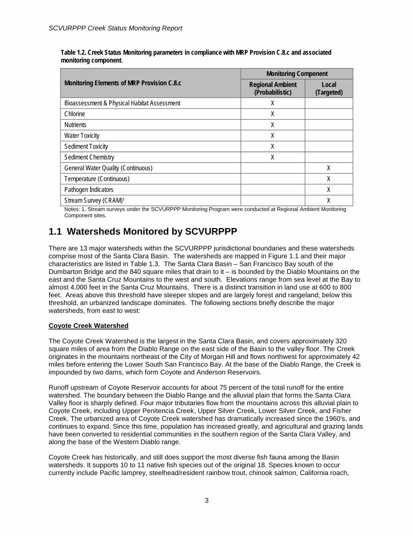
SCVURPPP Creek Status Monitoring Report
Table 1.2. Creek Status Monitoring parameters in compliance with MRP Provision C.8.c and associated monitoring component.
Monitoring Elements of MRP Provision C.8.c Monitoring Component
Regional Ambient (Probabilistic)
Local (Targeted)
Bioassessment & Physical Habitat Assessment X Chlorine X Nutrients X Water Toxicity X Sediment Toxicity X Sediment Chemistry X General Water Quality (Continuous) X
Temperature (Continuous) X Pathogen Indicators X Stream Survey (CRAM)1 X Notes: 1. Stream surveys under the SCVURPPP Monitoring Program were conducted at Regional Ambient Monitoring Component sites.
1.1 Watersheds Monitored by SCVURPPP There are 13 major watersheds within the SCVURPPP jurisdictional boundaries and these watersheds comprise most of the Santa Clara Basin. The watersheds are mapped in Figure 1.1 and their major characteristics are listed in Table 1.3. The Santa Clara Basin – San Francisco Bay south of the Dumbarton Bridge and the 840 square miles that drain to it – is bounded by the Diablo Mountains on the east and the Santa Cruz Mountains to the west and south. Elevations range from sea level at the Bay to almost 4,000 feet in the Santa Cruz Mountains. There is a distinct transition in land use at 600 to 800 feet. Areas above this threshold have steeper slopes and are largely forest and rangeland; below this threshold, an urbanized landscape dominates. The following sections briefly describe the major watersheds, from east to west:
Coyote Creek Watershed
The Coyote Creek Watershed is the largest in the Santa Clara Basin, and covers approximately 320 square miles of area from the Diablo Range on the east side of the Basin to the valley floor. The Creek originates in the mountains northeast of the City of Morgan Hill and flows northwest for approximately 42 miles before entering the Lower South San Francisco Bay. At the base of the Diablo Range, the Creek is impounded by two dams, which form Coyote and Anderson Reservoirs.
Runoff upstream of Coyote Reservoir accounts for about 75 percent of the total runoff for the entire watershed. The boundary between the Diablo Range and the alluvial plain that forms the Santa Clara Valley floor is sharply defined. Four major tributaries flow from the mountains across this alluvial plain to Coyote Creek, including Upper Penitencia Creek, Upper Silver Creek, Lower Silver Creek, and Fisher Creek. The urbanized area of Coyote Creek watershed has dramatically increased since the 1960's, and continues to expand. Since this time, population has increased greatly, and agricultural and grazing lands have been converted to residential communities in the southern region of the Santa Clara Valley, and along the base of the Western Diablo range.
Coyote Creek has historically, and still does support the most diverse fish fauna among the Basin watersheds. It supports 10 to 11 native fish species out of the original 18. Species known to occur currently include Pacific lamprey, steelhead/resident rainbow trout, chinook salmon, California roach,
3

SCVURPPP Creek Status Monitoring Report
hitch, Sacramento blackfish, Sacramento pikeminnow, Sacramento sucker, threespine stickleback, prickly sculpin, riffle sculpin, staghorn sculpin, and tule perch.
Lower Penitencia Creek Watershed
The Lower Penitencia Creek Watershed covers an area of about 30 square miles, half of which is on the western slopes of the Diablo Mountain Range on the east side of the Santa Clara Basin, and the other half on the valley floor. The major tributaries joining the Lower Penitencia Creek are the East Penitencia Channel and Berryessa Creek.
Lower Penitencia Creek flows from the foothills of the Diablo Range, through undeveloped, unincorporated County land, and continues westerly through largely residential neighborhoods in the Cities of Milpitas and San Jose, transitioning to higher density residential neighborhoods and industrial areas west of Interstate 680.
No native fish communities have been identified in Lower Penitencia Creek watershed.
Guadalupe River Watershed
The Guadalupe River Watershed covers an area of approximately 171 square miles. The headwaters lie in the eastern Santa Cruz Mountains near the summit of Loma Prieta. The Guadalupe River actually begins on the Valley floor at the confluence of Alamitos Creek and Guadalupe Creek, just downstream of Coleman Road in San Jose. From here it flows north, approximately 14 miles until it flows into the Lower South San Francisco Bay via Alviso Slough. On its journey, the Guadalupe River traverses through the town of Los Gatos, and the Cities of San Jose, Campbell, and Santa Clara, and is joined by three other tributaries: Ross, Canoas, and Los Gatos Creeks. The upper watershed is characterized by heavily forested areas with pockets of scattered residential areas. Residential density gradually increases to high density on the valley floor. Commercial development is focused along major surface streets. Industrial developments are located closer to the Bay, primarily downstream of the El Camino Real crossing. Six major reservoirs exist in the watershed: Calero Reservoir on Calero Creek, Guadalupe Reservoir on Guadalupe Creek, Almaden Reservoir on Alamitos Creek, Vasona Reservoir, Lexington Reservoir, and Lake Elsman on Los Gatos Creek. Guadalupe River watershed supports both warm and cold water native fish. Although much of the river is dominated by nonnative fish species, nine native fish species have been collected and/or observed during the last 20 years, including: Pacific lamprey, rainbow/steelhead trout, Chinook salmon, hitch, California roach, Sacramento sucker, threespine stickleback, riffle sculpin, and prickly sculpin. The Guadalupe River supports a reproducing steelhead trout population, as well as a small run of Chinook salmon.
San Tomas Aquino Creek Watershed
The San Tomas Aquino Creek Watershed covers an area of approximately 45 square miles. San Tomas Creek originates in the forested foothills of the Santa Cruz Mountains flowing in a northern direction through the cities of Campbell and Santa Clara, into Guadalupe Slough, and finally into Lower South San Francisco Bay. The major tributaries to San Tomas Aquino Creek include Saratoga, Wildcat, Smith and Vasona Creeks. Of these, Saratoga Creek drains the largest area 17 square miles) and joins San Tomas Creek 1.5 miles upstream of Highway 101. Due to its relatively large size, the Saratoga Creek subwatershed is often viewed as a distinct watershed even though it does not directly drain to Lower South San Francisco Bay.
Most of the San Tomas Aquino watershed is developed as high-density residential neighborhoods, with additional areas developed for commercial and industrial uses The majority of the San Tomas Aquino Creek channel has been modified and lined with concrete (from the Smith Creek confluence in the upper reaches downstream to Highway 101).Hitch is the only native fish found in San Tomas Aquino Creek.
Saratoga Creek, a major tributary to San Tomas Aquino Creek originates on the northeastern slopes of the Santa Cruz Mountains along Castle Rock Ridge at 3,100 feet in elevation. Saratoga creek flows for
4
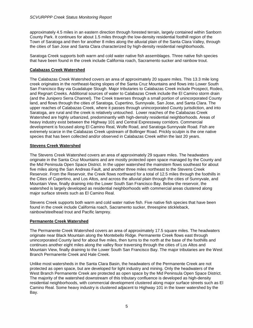
SCVURPPP Creek Status Monitoring Report
approximately 4.5 miles in an eastern direction through forested terrain, largely contained within Sanborn County Park. It continues for about 1.5 miles through the low-density residential foothill region of the Town of Saratoga and then for another 8 miles along the alluvial plain of the Santa Clara Valley, through the cities of San Jose and Santa Clara characterized by high-density residential neighborhoods.
Saratoga Creek supports both warm and cold water native fish assemblages. Three native fish species that have been found in the creek include California roach, Sacramento sucker and rainbow trout.
Calabazas Creek Watershed
The Calabazas Creek Watershed covers an area of approximately 20 square miles. This 13.3 mile long creek originates in the northeast-facing slopes of the Santa Cruz Mountains and flows into Lower South San Francisco Bay via Guadalupe Slough. Major tributaries to Calabazas Creek include Prospect, Rodeo, and Regnart Creeks. Additional sources of water to Calabazas Creek include the El Camino storm drain (and the Junipero Serra Channel). The Creek traverses through a small portion of unincorporated County land, and flows through the cities of Saratoga, Cupertino, Sunnyvale, San Jose, and Santa Clara. The upper reaches of Calabazas Creek, where it passes through unincorporated County jurisdiction, and into Saratoga, are rural and the creek is relatively untouched. Lower reaches of the Calabazas Creek Watershed are highly urbanized, predominantly with high-density residential neighborhoods. Areas of heavy industry exist between the Highway 101 and Central Expressway corridors. Commercial development is focused along El Camino Real, Wolfe Road, and Saratoga-Sunnyvale Road. Fish are extremely scarce in the Calabazas Creek upstream of Bollinger Road. Prickly sculpin is the one native species that has been collected and/or observed in Calabazas Creek within the last 20 years.
Stevens Creek Watershed
The Stevens Creek Watershed covers an area of approximately 29 square miles. The headwaters originate in the Santa Cruz Mountains and are mostly protected open space managed by the County and the Mid Peninsula Open Space District. In the upper watershed the mainstem flows southeast for about five miles along the San Andreas Fault, and another three miles northeast to the Stevens Creek Reservoir. From the Reservoir, the Creek flows northward for a total of 12.5 miles through the foothills in the Cities of Cupertino, and Los Altos, and across the alluvial plain through the cities of Sunnyvale, and Mountain View, finally draining into the Lower South San Francisco Bay. Below the reservoir, the watershed is largely developed as residential neighborhoods with commercial areas clustered along major surface streets such as El Camino Real.
Stevens Creek supports both warm and cold water native fish. Five native fish species that have been found in the creek include California roach, Sacramento sucker, threespine stickleback, rainbow/steelhead trout and Pacific lamprey.
Permanente Creek Watershed
The Permanente Creek Watershed covers an area of approximately 17.5 square miles. The headwaters originate near Black Mountain along the Montebello Ridge. Permanente Creek flows east through unincorporated County land for about five miles, then turns to the north at the base of the foothills and continues another eight miles along the valley floor traversing through the cities of Los Altos and Mountain View, finally draining to the Lower South San Francisco Bay. The major tributaries are the West Branch Permanente Creek and Hale Creek.
Unlike most watersheds in the Santa Clara Basin, the headwaters of the Permanente Creek are not protected as open space, but are developed for light industry and mining. Only the headwaters of the West Branch Permanente Creek are protected as open space by the Mid Peninsula Open Space District. The majority of the watershed downstream of this tributary confluence is developed as high-density residential neighborhoods, with commercial development clustered along major surface streets such as El Camino Real. Some heavy industry is clustered adjacent to Highway 101 in the lower watershed by the Bay.
5

SCVURPPP Creek Status Monitoring Report
Four species of native fishes have been collected and/or observed from Permanente Creek during the last 20 years: rainbow trout, California roach, Sacramento sucker, and threespine stickleback. The native fish assemblage primarily occurs in the reaches upstream of Interstate 280.
Adobe Creek Watershed
The Adobe Creek Watershed covers an area of approximately 10 square miles, of which roughly 7.5 square miles are mountainous and 2.5 square miles are on the valley floor. Adobe Creek originates on the northeastern facing slopes of the Santa Cruz Mountains and flows northerly over steep forested terrain until it meets the Middle, West and North Adobe Forks. Other major tributaries in the upper watershed are Moody and Purissima Creeks.
The drainage area above the confluence of the Adobe Forks is undeveloped open space. The remainder of the watershed primarily consists of residential development. Along the valley floor, Adobe Creek flows through Los Altos Hills, Los Altos, Palo Alto, and Mountain View. Adobe Creek is joined by Barron Creek west of Highway 101 and continues to flow through estuarine area with tidal influence until it drains into the Palo Alto Flood Basin and then the Lower South San Francisco Bay.
Four species of native fishes have been collected from Adobe Creek: California roach, Sacramento sucker, threespine stickleback, and prickly sculpin.
Matadero Creek Watershed
The Matadero Creek watershed covers an area of about 14 square miles, of which approximately 11 square miles are mountainous land, and 3 square miles are gently sloping valley floor. Matadero Creek originates in the foothills of the Santa Cruz Mountains and flows in a northeasterly direction for approximately eight miles until it discharges into the Palo Alto Flood Basin, and then drains into the Lower South San Francisco Bay. Major tributaries to Matadero Creek are Arastradero and Deer Creeks and Stanford Channel.
Through the foothills, Matadero Creek traverses through low-density residential development in the town of Los Altos Hills. As it nears the valley floor, it flows through the Stanford University Preserve and Campus, and then through residential, commercial, and industrial areas of Palo Alto. The portions of the watershed that fall in the northern part of the City of Palo Alto are predominantly residential, commercial and public/institutional.
Five species of native fishes have been collected and/or observed from Matadero Creek during the last 20 years: California roach, Sacramento blackfish, Sacramento sucker, threespine stickleback, and prickly sculpin.
Barron Creek Watershed
The Barron Creek Watershed covers an area of approximately three square miles of urban development between the Matadero and Adobe Creek watersheds. Barron Creek is approximately 5 miles long, originating in the low-density residential foothill region of the Town of Los Altos Hills and flowing in a northeasterly direction through residential, commercial, and industrial areas within the City of Palo Alto. The Creek joins neighboring Adobe Creek just upstream of Highway 101 and drains via a tide gate to the Lower South San Francisco Bay through the Palo Alto Flood Basin. It has no major tributaries.
Barron Creek has been greatly modified for flood control purposes; approximately 67 percent of the total length of creek bed has been hardened. Upstream of El Camino Real the creek is piped for much of its length. Natural channel sections occur immediately adjacent to Arastradero Road and at the Barron Creek Debris Basin. Downstream of El Camino Real, Barron Creek is contained in a concrete trapezoidal channel. During large storm events, high flows from Barron Creek may be diverted to Matadero Creek via the Barron Creek Bypass structure. No native fish communities have been identified upstream of the tidally influenced area of the creek.
6

SCVURPPP Creek Status Monitoring Report
San Francisquito Creek Watershed
San Francisquito Creek and its tributaries drain 47.5 square miles in northwestern Santa Clara and southeastern San Mateo counties. The watershed is bounded to the southwest by the Santa Cruz Mountains. San Francisquito Creek itself flows 12.5 miles from Searsville Dam to the Lower South San Francisco Bay and defines the border between San Mateo and Santa Clara Counties. San Francisquito Creek traverses unincorporated County, Stanford University land, the towns of Portola Valley and Woodside, as well as the cities of Menlo Park, Palo Alto, and East Palo Alto.
The upper watershed is comprised of undeveloped forest and grazing lands and low-density residential neighborhoods. On the valley floor, higher-density residential development exists along with commercial development focused on major surface streets. Stanford University occupies a large portion of the valley portion of the watershed as does the downtown portion of the City of Palo Alto.
The watershed is famous for its reproducing steelhead population. Besides steelhead, native fish found in the watershed are the California roach, Sacramento sucker, hitch, speckled dace, threespined stickleback, and prickly sculpin. Seven nonnative species also exist in the watershed. The threatened California red-legged frog lives along the Creek.
Sunnyvale East Channel
The Sunnyvale East Channel was constructed in 1967 to manage flooding that was becoming a problem due to subsidence of lands in the drainage area. The Sunnyvale East Channel watershed covers 7.1 square miles extending from central Cupertino northeastward through the City of Sunnyvale. The watershed draining to the Channel is located entirely on the alluvial plain of the Santa Clara Valley. The Channel is approximately 6 miles in length and extends from Interstate 280 in the south to Guadalupe Slough in the north. The channel is a man-made feature with no natural antecedent. One quarter of it runs through underground culverts. It drains to the Lower South San Francisco Bay via the Junipero Serra Channel and the Guadalupe Slough.
The Sunnyvale East Channel watershed is almost entirely urbanized with predominately residential development (59%), as well as commercial and industrial (23%). (SCVWD 2005b) The only contiguous open space area in the watershed is the Sunnyvale Baylands along the San Francisco Bay shoreline and smaller city-owned parks in Sunnyvale and Cupertino. No fish species are known to occur upstream of the tidally influenced area.
Sunnyvale West Channel
The Sunnyvale West Channel was constructed in 1964 to manage flooding that was becoming a problem due to subsidence of lands in the drainage area. The Channel watershed drains 7.5 square miles and is entirely located on the alluvial plain of the Santa Clara Valley. The channel originates in the urbanized sections of Sunnyvale and Mountain View. The Channel is approximately 3 miles in length, extending from Guadalupe Slough to Maude Avenue (SCVWD 2005b). From the upper end of the channel at Maude Avenue to Almanor Avenue, the Sunnyvale West Channel is a concrete pipe culvert. Downstream of Almanor Avenue to Mathilda Avenue, the channel is an earth-excavated channel. Sunnyvale West Channel drains to Lower South San Francisco Bay via the Moffett Channel and then the Guadalupe Slough.
The Sunnyvale West Channel watershed is almost entirely urbanized with mostly public/institutional development (31%), as well as industrial (25%) and residential (23%) areas (SCVWD 2005b). The only open space in the watershed is the Sunnyvale Baylands along the San Francisco Bay shoreline and several smaller city-owned parks in Sunnyvale. No fish species are known to occur upstream of the tidally influenced area.
7

SCVURPPP Creek Status Monitoring Report
Table 1.3. Characteristics of major watersheds within SCVURPPP boundary.
Watershed Area
(square miles)
Number of
Tributary Creeks
Natural Creek Bed
(Miles)
Engineered Channel (Miles)
Underground Culvert or
Stormdrain (Miles)
Impervious Area
Land Use
Residential Industrial/ Commercial Forest Rangeland Other
Adobe 11.0 7 18.8 2.3 12.0 44.7% 46.5% 11.8% 36.3% 2.7% 2.7% Barron 15.6 5 15.1 7.9 28.6 60.3% 60.5% 20.1% 7.3% 7.0% 5.1% Calabazas 20.3 6 12.9 14.1 55.5 NA 54.5% 29.4% 8.8% 5.2% 2.1% Coyote 321 53 670 36.4 146 11.1% 8.6% 3.7% 49.9% 29.6% 8.2% Guadalupe 171 50 207 45.5 265 37.1% 29.6% 13.6% 34.7% 15.5% 6.6% Lower Penitencia 28.6 13 29.2 20.8 61.6 42.9% 30.7% 19.0% 1.1% 38.7% 10.5% Matadero 14.0 3 18 NA NA 60.3% 57.1% 5.8% 8.9% 8.2% 20% Permanente 17.3 7 NA NA NA 43.9% 46.3% 13.1% 35.0% 2.8% 2.8% San Francisquito 42.8 25 90.6 4.8 15.3 20.8% 29.6% 5.2% 44.7% 15.0% 5.5% San Tomas Aquino 44.8 15 50.5 15.5 79.3 60.1% 53.9% 18.8% 23.7% 0.8% 2.8% Stevens 29.2 12 54.2 1.1 30.0 28.6% 24.5% 9.0% 49.2% 12.5% 4.8% Sunnyvale East 7.1 0 0 6.2 26.6 82.2% 65.3% 31.8% 0% 0% 2.9% Sunnyvale West 7.6 0 0 6.7 18.7 72.4% 20.9% 65.2% 0% 0% 13.9% Source: http://www.scvurppp-w2k.com/watersheds.shtml NA – not available
8

SCVURPPP Creek Status Monitoring Report
Figure 1.1. Watersheds within SCVURPPP jurisdictional boundaries.
9

SCVURPPP Creek Status Monitoring Report
1.2 Designated Beneficial Uses Beneficial Uses in Santa Clara Valley creeks are designated by the SFRWQCB for specific water bodies and generally apply to all its tributaries. Uses include aquatic life, recreation, human consumption, and habitat. Table 1.4 lists Beneficial Uses designated by the SFRWQCB (2013) for water bodies monitored by SCVURPPP in Water Year 2014.
Table 1.4. Creeks monitored by SCVURPPP in Water Year 2014 and their Beneficial Uses (SFRWQCB 2013).
Waterbody
AGR
MUN
FRSH
GWR
IND
PROC
COMM
SHEL
L
COLD
EST
MAR
MIGR
RARE
SPW
N
WAR
M
WIL
D
REC-
1
REC-
2
NAV
Adobe Creek E E E E E Arroyo Aguague Creek E E E E E E E E Arroyo Calero E E E E E E E E E Arroyo de las Coches E E E E E Austrian Gulch Creek E E E E E E E Calera Creek E E E E Canoas Creek E E E E Guadalupe Creek E E E E E E E E E E
Guadalupe River E E E E E E E E E
Los Gatos Creek E E E E P E P E E E P Lower Silver Creek E E E E Ross Creek E E E E E San Tomas Aquino Creek E E E E E E
Saratoga Creek E E E E E E E E
Stevens Creek E E E E E E E E E E
Thompson Creek E E E E Notes:
COLD = Cold Fresh Water Habitat NAV = Navigation WARM = Warm Freshwater Habitat FRSH = Freshwater Replenishment RARE= Preservation of Rare and WILD = Wildlife Habitat GWR - Groundwater Recharge Endangered Species P = Potential Use MIGR = Fish Migration REC-1 = Water Contact Recreation E = Existing Use MUN = Municipal and Domestic Water REC-2 = Non-contact Recreation L = Limited Use.
* = “Water quality objectives apply; water contact recreation is prohibited or limited to protect public health” (SFRWQCB 2013).
EST = Estuarine (the Basin Plan assigns this beneficial use to slough portions of Plummer Creek; for this evaluation WARM is presumed applicable to freshwater portions)
The remainder of this report describes the two components of the monitoring design (targeted and probabilistic) (Section 2.0); monitoring methods (Section 3.0); data analysis and interpretation methods (Section 4.0); results and discussion, including a statement of data quality, biological condition assessment, and stressor analysis (Section 5.0), and summary conclusions (Section 6.0).
10

SCVURPPP Creek Status Monitoring Report
2.0 MONITORING DESIGN 2.1 Targeted Monitoring Design During Water Year 2014 (WY2014; October 1, 2013 – September 30, 2014) water temperature, general water quality, and pathogen indicators were monitored at selected sites using a targeted monitoring design based on the directed principle4 to address the following management questions:
1. What is the spatial and temporal variability in water quality conditions during the spring and summer season?
2. Do general water quality measurements indicate potential impacts to aquatic life?
3. What are the pathogen indicator concentrations at creek sites where there is potential for water contact recreation to occur?
4. What are the riparian conditions at bioassessment sampling stations? Are riparian assessments good indicators for condition of aquatic life use? Can they help identify stressors to aquatic life uses?
2.1.1 Targeted Site Selection General Water Quality
General water quality data (dissolved oxygen, specific conductance, pH, and temperature) were collected at a total of three locations in the Stevens Creek watershed during WY2014 (Table 2.3, Figure 2.3). Two of the sampling stations were located at probabilistic sites (i.e., bioassessment sampling locations in 2014) within the urban area below Stevens Creek Reservoir. These locations were selected to provide water quality data in a reach that supports both rearing and spawning habitat for the existing steelhead population. A third sampling location was established near the urban boundary approximately three miles upstream of the Stevens Creek Reservoir. The upper station was selected to provide water quality data in a perennial reach of the creek upstream of the reservoir.
Temperature
Water temperature was monitored at five sites within the Stevens Creek watershed and at five sites within the Guadalupe Creek watershed during WY2014. Both creeks have dams at the base of the Santa Cruz Mountain foothills that are operated by the Santa Clara Valley Water District, primarily for ground water percolation during the dry season. Temperature stations were located both above and below reservoirs. Both creeks support rainbow trout/steelhead populations, as well as other native fishes.
Three of the five sites in Stevens Creek were located downstream of the Stevens Creek Reservoir; one site at Blackberry Farm; one site at McClellan Ranch and one site at stream gage within Lower Stevens Creek County Park. These locations were selected to provide temperature data in a reach that supports both rearing and spawning habitat for existing steelhead population. The remaining two sites were upstream of the reservoir; one site at the Sycamore Group Picnic Area and the other site adjacent to Stevens Creek Canyon Road (approximately 3 miles upstream of the reservoir). The upper station was selected to provide temperature data in perennial section of the creek upstream of the reservoir.
In Guadalupe Creek, water temperature was monitored at four locations below the Guadalupe Reservoir; one site downstream of Camden and Coleman intersection; one site at the stream gage near Shannon Oaks Lane; one site below the fish ladder; and one site approximately 0.5 mile downstream of the
4 Directed Monitoring Design Principle: A deterministic approach in which points are selected deliberately based on knowledge of their attributes of interest as related to the environmental site being monitored. This principle is also known as "judgmental," "authoritative," "targeted," or "knowledge-based."
11

SCVURPPP Creek Status Monitoring Report
reservoir. All three sites are located in a reach of Guadalupe Creek that can potentially support both rearing and spawning habitat for steelhead. The remaining site was located directly below the confluence of Rincon Creek, which was selected to provide temperature data in the reach upstream of the reservoir.
Pathogen Indicators
Pathogen indicator samples were collected at five sites located in municipal or county owned parks in areas with good public access to creeks and potential for recreational water contact. The five stations were also bioassessment sites sampled in WY2014.
2.2 Probabilistic Monitoring Design Targeted monitoring may not give an accurate view of background conditions because site selection is biased toward sites where historical or existing water quality concerns have been identified. Therefore, the RMC augments targeted monitoring designs with an ambient (probabilistic) creek status design that was developed to remove bias from site selection. This design allows each individual RMC participating program to objectively assess stream ecosystem conditions within its program area (County boundary) while contributing data to answer regional management questions about water quality and beneficial use condition in San Francisco Bay Area creeks.
The RMC regional probabilistic monitoring design was developed to address the management questions listed below:
1. What is the condition of aquatic life in creeks in the RMC area; are water quality objectives met and are beneficial uses supported?
i. What is the condition of aquatic life in the urbanized portion of the RMC area; are water quality objectives met and are beneficial uses supported?
ii. What is the condition of aquatic life in RMC participant counties; are water quality objectives met and are beneficial uses supported?
iii. To what extent does the condition of aquatic life in urban and non-urban creeks differ in the RMC area?
iv. To what extent does the condition of aquatic life in urban and non-urban creeks differ in each of the RMC participating counties?
2. What are major stressors to aquatic life in the RMC area?
i. What are major stressors to aquatic life in the urbanized portion of the RMC area?
3. What are the long-term trends in water quality in creeks over time? These questions will be addressed for the RMC area after a suitable number of sites have been sampled, which is expected to occur after 3 or 4 years.
Table 2.1 illustrates the total number of sites that each RMC Permittee planned to sample within the MRP term at the outset of the monitoring program, including sampling efforts planned by SFRWQCB (approximately 2 sites per county per year). Approximately 80 percent of the sites are in urban areas and 20 percent are in non-urban areas5. Table 2.1 also illustrates the number of sampling years required to establish statistically representative sample sizes (30 samples) for each of the classified strata in the regional monitoring design6. In Santa Clara County, a statistically representative sample of urban sites
5 Some sites classified as urban, using the GIS may be considered for reclassification as non-urban based on actual land uses of the drainage area despite location inside municipal jurisdictional boundaries. 6 For each of the strata, it is necessary to obtain a sample size of at least 30 in order to evaluate the condition of aquatic life within known estimates of precision. This estimate is defined by a power curve from a binomial distribution (BASMAA 2014a).
12

SCVURPPP Creek Status Monitoring Report
was anticipated in Year 2 (WY2013) of the program. A statistically representative sample of non-urban sites is not anticipated until Year 5 (WY2016) of the program. Due to unforeseen field circumstances, the actual number of sites sampled and the percentage of urban and non-urban sites may vary. Such outcomes can be addressed in subsequent sampling years.
Table 2.1. Projected number of samples per monitoring yeara; shaded cells indicate when a minimum sample size may be available to develop a statistically representative data set to address management questions related to condition of aquatic life.
Monitoring Year
RMC Area (Region-wide)
Santa Clara County
Alameda County
Contra Costa County
San Mateo County
Fairfield, Suisun City and
Vallejo b
Land Use Urban Non-Urban Urban Non-
Urban Urban Non-Urban Urban Non-
Urban Urban Non-Urban Urban Non-
Urban
Year 1 (WY2012) 48 22 16 6 16 6 8 4 8 4 0 2
Year 2 (WY2013) 100 44 32 12 32 12 16 8 16 8 4 4
Year 3
(WY2014) 156 66 48 18 48 18 24 12 24 12 12 6
Year 4 (WY2015) 204 88 64 24 64 24 32 16 32 16 12 8
Year 5 (WY2016) 256 110 80 30 80 30 40 20 40 20 16 10
a Assumes SFRWQCB samples two non-urban sites annually in each RMC County. b Assumes: FSURMP and Vallejo only monitor urban sites; FSURMP monitors 4 sites in Year 2, 3 and 5; and Vallejo monitors 4 sites in Year 3.
2.2.1 RMC Area The RMC area encompasses 3,407 square miles of land in the San Francisco Bay Area. This includes the portions of the five participating counties that fall within the San Francisco Bay Regional Water Quality Control Board (SFRWQCB) boundary, as well as the eastern portion of Contra Costa County that drains to the Central Valley region (Figure 2.1). Creek status and trends monitoring is being conducted in non-tidally influenced, flowing water bodies (i.e., creeks, streams and rivers) interspersed among the RMC area. The water bodies monitored were drawn from a master list that included all perennial and non-perennial creeks and rivers that run through both urban and non-urban areas within the RMC area.
13

SCVURPPP Creek Status Monitoring Report
Figure 2.1. Map of BASMAA RMC area showing each member program’s boundary and urban and non-urban areas.
2.2.2 Probabilistic Site Selection The regional probabilistic design was developed using the Generalized Random Tessellation Stratified (GRTS) approach developed by the United States Environmental Protection Agency (USEPA) and Oregon State University (Stevens and Olson 2004). GRTS offers multiple benefits for coordinating amongst monitoring entities including the ability to develop a spatially balanced design that produces statistically representative data with known confidence intervals. The GRTS approach has been implemented recently in California by several agencies including the statewide Perennial Streams Assessment (PSA) conducted by SWAMP (Ode et al. 2011) and the Southern California Stormwater Monitoring Coalition’s (SMC) regional monitoring program conducted by municipal stormwater programs in Southern California (SMC 2007). For the purpose of developing the RMC’s probabilistic design, the 3,407-square mile RMC area is considered to represent the “sample universe.”
Sample sites were selected and attributed using the GRTS approach from a sample frame consisting of a creek network geographic information system (GIS) data set within the RMC boundary (BASMAA 2012). This approach was agreed to by SFRWQCB staff during RMC workgroup meetings although it differs from that specified in MRP Provision C.8.c.iv., e.g., sampling on the basis of individual watersheds in rotation and selecting sites to characterize segments of a waterbody(s). The sample frame includes non-
14

SCVURPPP Creek Status Monitoring Report
tidally influenced perennial and non-perennial creeks within five management units representing areas managed by the storm water programs associated with the RMC. The sample frame was stratified by management unit to ensure that MRP Provision C.8.c sample size requirements (SFRWQCB 2009) would be achieved.
The National Hydrography Plus Dataset (1:100,000) was selected as the creek network data layer to provide consistency with both the Statewide PSA and the SMC, and the opportunity for future data coordination with these programs. The RMC sample frame was classified by county and land use (i.e., urban and non-urban) to allow for comparisons between these strata. Urban areas were delineated by combining urban area boundaries and city boundaries defined by the U.S. Census (2000). Non-urban areas were defined as the remainder of the areas within the sample universe (i.e., RMC area). Some sites classified as urban fall near the non-urban edge of the city boundaries and have little upstream development. For the purposes of consistency, these urban sites were not re-classified. Therefore, data values within the urban classification represent a wide range of conditions.
Based on discussion during RMC Workgroup meetings, with SFRWQCB staff present, RMC participants weighted their sampling efforts so that annual sampling efforts are approximately 80% in urban areas and 20% in non-urban areas for the purpose of comparison. RMC participants coordinated with the SFRWQCB by identifying additional non-urban sites from their respective counties and providing a list of sites for SWAMP to conduct site evaluations. Since 2012, the SFRWQCB has supplemented the RMC monitoring efforts with 34 additional non-urban probabilistic sites within RMC jurisdiction. The total number of sites has been variable each year, with 6 sites in WY2012, 18 sites in WY2013 and 10 sites in WY2014. Information from these sampling events is included in the Site Evaluation summary (Section 2.2.3) but not included in either the results or discussion sections of this report.
2.2.3 Site Evaluation Sites identified in the regional sample draw were evaluated by each RMC participant in chronological order using a two-step process described in RMC Standard Operating Procedure FS-12 (BASMAA 2014b), consistent with the procedure described by Southern California Coastal Water Research Project (SCCWRP) (2012). Each site was evaluated to determine if it met the following RMC sampling location criteria:
1. The location (latitude/longitude) provided for a site is located on or is within 300 meters of a non-impounded receiving water body7;
2. Site is not tidally influenced;
3. Site is wadeable during the sampling index period;
4. Site has sufficient flow during the sampling index period to support standard operation procedures for biological and nutrient sampling.
5. Site is physically accessible and can be entered safely at the time of sampling;
6. Site may be physically accessed and sampled within a single day;
7. Landowner(s) grant permission to access the site8.
In the first step, these criteria were evaluated to the extent possible using a “desktop analysis.” Site evaluations were completed during the second step via field reconnaissance visits. Based on the outcome of site evaluations, sites were classified into one of three categories:
7 The evaluation procedure permits certain adjustments of actual site coordinates within a maximum of 300 meters. 8 If landowners did not respond to at least two attempts to contact them either by written letter, email, or phone call, permission to access the respective site was effectively considered to be denied.
15

SCVURPPP Creek Status Monitoring Report
• Target – Target sites were grouped into two subcategories:
o Target Sampleable (TS) - Sites that met all seven criteria and were successfully sampled.
o Target Non-Sampleable (TNS) - Sites that met criteria 1 through 4, but did not meet at least one of criteria 5 through 7 were classified as TNS.
• Non-Target (NT) - Sites that did not meet at least one of criteria 1 through 4 were classified as non-target status.
• Unknown (U) - Sites were classified with unknown status when it could be reasonably inferred either via desktop analysis or a field visit that the site was a valid receiving water body and information for any of the seven criteria was unconfirmed.
Table 2.2 lists the total number of sites evaluated in Santa Clara County between WY2012 and WY2014, and their classification categories. A handful of the sites classified as non-urban were evaluated by the SFRWQCB for potential SWAMP sampling. Results of the site evaluation are illustrated in Figure 2.2 and described in further detail in Attachment A.
Table 2.2. Results of Probabilistic Site Evaluations for WY2012 through WY2014 by SCVURPPP.
Classification WY2012 WY2013 WY2014 TOTAL
# of Sites % # of
Sites % # of Sites % # of
Sites %
Target Sampleable (TS) 21 39 23 29 25 21 69 28 Target Non-Sampleable (TNS) 16 30 18 23 13 11 47 19 Non-Target (NT) 17 31 37 47 55 46 109 43 Unknown (U) -- -- -- -- 26 22 26 10 TOTAL SITES EVALUATED 54 100 78 100 119 100 251 100
Figure 2.2. Results of Santa Clara County site evaluations for Water Years 2012-2014.
The complete list of target and probabilistic monitoring sites sampled by SCVURPPP in WY2014 is presented in Table 2.3. Monitoring locations with monitoring parameter(s) and year sampled are shown in Figure 2.3.
28%
19%43%
10%
Target Sampleable (TS)Target Non-Sampleable (TNS)Non-Target (NT)Unknown (U)
16

DRAFT DRAFT
SCVURPPP Creek Status Monitoring Report
Figure 2.3. Map of SCVURPPP Program Area, major creeks, and sites monitored in WY2014.
17

SCVURPPP Creek Status Monitoring Report
Table 2.3. Sites and parameters monitored in WY2014 in Santa Clara County.
Map ID
Station Number Watershed Creek Name Land
Use Latitude Longitude
Probabilistic Monitoring Targeted Monitoring
Bioassessment, Nutrients,
General WQ
Toxicity, Sediment Chemistry
CRAM Temp Cont WQ
Pathogen Indicators
266 205R00266 Guadalupe River Limekiln Creek NU 37.20297 -121.97351 x x 330 205R00330 Guadalupe River Hick's Creek NU 37.19825 -121.90036 x x 362 205R00362 Guadalupe River Lyndon Canyon NU 37.21993 -122.05424 x x 394 205R00394 Guadalupe River Austrian Gulch NU 37.13783 -121.92191 x x 851 205R00851 Lower Penitencia Creek Los Coches Creek U 37.43828 -121.87107 x x 883 205R00883 Adobe Creek Adobe Creek U 37.37108 -122.11822 x x x 915 205R00915 Coyote Creek Thompson Creek U 37.31356 -121.79463 x x 938 205R00938 San Tomas Aquino San Tomas Aquino Creek U 37.26063 -121.99153 x x x 979 205R00979 Coyote Creek Lower Silver Creek U 37.35479 -121.84920 x x x 1027 205R01027 Guadalupe River Guadalupe River U 37.35753 -121.91463 x x 1091 205R01091 Saratoga Creek Saratoga Creek U 37.35815 -121.97311 x x x 1098 205R01098 Guadalupe River Guadalupe Creek U 37.21056 -121.90357 x x 1187 205R01187 Stevens Creek Stevens Creek U 37.30044 -122.07617 x x x 1226 205R01226 Guadalupe River Los Gatos Creek U 37.29708 -121.93080 x x 1299 205R01299 Coyote Creek Arroyo Aguague U 37.39781 -121.78597 x x 1306 205R01306 Guadalupe River Ross Creek U 37.24872 -121.91370 x x 1434 205R01434 Guadalupe River Arroyo Calero U 37.21388 -121.83368 x x x 1443 205R01443 Stevens Creek Stevens Creek U 37.31478 -122.06098 x x x 1539 205R01539 Guadalupe River Los Gatos Creek U 37.31390 -121.90366 x x x 1578 205R01578 San Tomas Aquino San Tomas Aquino Creek U 37.24035 -122.00593 x x 64 205STE064 Stevens Creek Stevens Creek 37.31873 -122.06143 x 65 205STE065 Stevens Creek Stevens Creek 37.31321 -122.06412 x x 70 205STE070 Stevens Creek Stevens Creek 37.30592 -122.07321 x 71 205STE071 Stevens Creek Stevens Creek 37.30253 -122.07487 x 95 205STE095 Stevens Creek Stevens Creek 37.28269 -122.07527 x 10⁵ 205STE105 Stevens Creek Stevens Creek 37.26958 -122.09925 x x 205 205GUA205 Guadalupe River Guadalupe Creek 37.22685 -121.90283 x 210 205GUA210 Guadalupe River Guadalupe Creek 37.21748 -121.91031 x 213 205GUA213 Guadalupe River Guadalupe Creek 37.21018 -121.90386 x 218 205GUA218 Guadalupe River Guadalupe Creek 37.20280 -121.88845 x 229 205GUA229 Guadalupe River Guadalupe Creek 37.18241 -121.87341 x
18

SCVURPPP Creek Status Monitoring Report
3.0 MONITORING METHODS Water quality data were collected in accordance with SWAMP-comparable methods and procedures described in the BASMAA RMC Standard Operating Procedures (SOPs; BASMAA 2014b) and associated Quality Assurance Project Plan (QAPP; BASMAA 2014a). These documents and the RMC Creek Status and Long-Term Trends Monitoring Plan (BASMAA 2012) are updated as needed to maintain their currency and optimal applicability. Where applicable, monitoring data were collected using methods comparable to those specified by the California Surface Water Ambient Monitoring Program (SWAMP) QAPP9, and were submitted in SWAMP-compatible format to the SFRWQCB. The SOPs were developed using a standard format that describes health and safety cautions and considerations, relevant training, site selection, and sampling methods/procedures, including pre-fieldwork mobilization activities to prepare equipment, sample collection, and de-mobilization activities to preserve and transport samples. The SOPs relevant to the monitoring discussed in this report are listed in Table 3.1.
Table 3.1. Standard Operating Procedures (SOPs) pertaining to creek status monitoring.
SOP # SOP FS-1 Benthic Macroinvertebrate and Algae Bioassessments, and Physical Habitat Measurements FS-2 Water Quality Sampling for Chemical Analysis, Pathogen Indicators, and Toxicity Testing FS-3 Field Measurements, Manual FS-4 Field Measurements, Continuous General Water Quality FS-5 Continuous Temperature Measurements FS-6 Collection of Bedded Sediment Samples FS-7 Field Equipment Cleaning Procedures FS-8 Field Equipment Decontamination Procedures FS-9 Sample Container, Handling, and Chain of Custody Procedures FS-10 Completion and Processing of Field Datasheets FS-11 Site and Sample Naming Convention FS-12 Ambient Creek Status Monitoring Site Evaluation
3.1 Field Data Collection Methods
3.1.1 Bioassessments In accordance with the RMC QAPP (BASMAA 2014a) bioassessments were planned during the spring index period (approximately April 15 – July 15) with the goal to sample a minimum of 30 days after any significant storm (roughly defined as at least 0.5-inch of rainfall within a 24-hour period). During WY2014, a significant storm occurred on April 1st and bioassessments were initiated during the week of April 21st 2014, approximately 20 days following the last storm event. With guidance from SFRWQCB staff, bioassessments began prior to the 30 day grace period due to rapidly declining volume of spring flows and lack of sampleable sites as the result of an extended period of drought.
9The current SWAMP QAPP is available at: http://www.waterboards.ca.gov/water_issues/programs/swamp/docs/qapp/swamp_qapp_master090108a.pdf
19

SCVURPPP Creek Status Monitoring Report
Benthic Macroinvertebrates
Each bioassessment sampling site consisted of an approximately 150-meter stream reach that was divided into 11 equidistant transects placed perpendicular to the direction of flow. The sampling position within each transect alternated between 25%, 50% and 75% distance of the wetted width of the stream. Benthic macroinvertebrates (BMIs) were collected from a 1 square foot area approximately 1 m downstream of each transect (see SOP FS-1, BASMAA 2014b). The benthos were disturbed by manually rubbing coarse substrate followed by disturbing the upper layers of substrate to a depth of 4-6 inches to dislodge any remaining invertebrates into the net. Slack water habitat procedures were used at transects with deep and/or slow moving water (Ode 2007). Material collected from the eleven subsamples was composited in the field by transferring the entire sample into one or two 1000 ml wide-mouth jar(s) and preserving it with 95% ethanol.
Algae
Filamentous algae and diatoms were collected using the Reach-Wide Benthos (RWB) method described in SOP FS-1 (BASMAA 2014b). Algae samples were collected synoptically with and immediately after BMI sample collection. The sampling position within each transect was the same as used for BMI sampling; however, samples were collected six inches upstream of the BMI sampling position. The algae were collected using a range of methods and equipment, depending on the particular substrate occurring at the site (i.e., erosional, depositional, large and/or immobile, etc) per SOP FS-1. Erosional substrates included any material (substrate or organics) small enough to be removed from the stream bed, but large enough in size to isolate an area equal in size to a rubber delimiter (12.6 cm2 in area). When a sample location along a transect was too deep to sample, a more suitable location was selected, either on the same transect or from one further upstream.
Algae samples were collected at each transect prior to moving on to the next transect. Sample material (substrate and water) from all eleven transects was combined in a sample bucket, agitated, and a suspended algae sample was then poured into a 500 mL cylinder, creating a composite sample for the site. A 45 mL subsample was taken from the algae composite sample and combined with 5 mL glutaraldehyde into a 50 mL sample tube for taxonomic identification of soft algae. Similarly, a 40 mL subsample was extracted from the algae composite sample and combined with 10 mL of 10% formalin into a 50 mL sample tube for taxonomic identification of diatoms. Laboratory processing included identification and enumeration of 300 natural units of soft algae and 600 diatom valves to the lowest practical taxonomic level.
The algae composite sample was also used for collection of chlorophyll a and ash free dry mass (AFDM) samples following methods described in Fetscher et al (2009). For the chlorophyll a sample, 25 mL of the algae composite volume was removed and run through a glass fiber filter (47 mm, 0.7 um pore size) using a filtering tower apparatus. The AFDM sample was collected using a similar process using pre-combusted filters. Both samples were placed in whirlpaks, covered in aluminum foil and immediately placed on ice for transportation to laboratory.
3.1.2 Physical Habitat Physical habitat assessments (PHAB) were conducted at each BMI bioassessment sampling event using the PHAB protocols described in Ode (2007) (see SOP FS-1, BASMAA 2014b). Physical habitat data were collected at each of the 11 transects and at 10 additional inter-transects (located between each main transect) by implementing the “Basic” level of effort, with the following additional measurements/assessments as defined in the “Full” level of effort (as prescribed in the MRP): water depth and pebble counts, cobble embeddedness, flow habitat delineation, and instream habitat complexity. At algae sampling locations, additional assessment of presence of micro- and macroalgae was conducted during the pebble counts. In addition, water velocities were measured at a single location in the sample reach (when possible) using protocols described in Ode (2007).
20

SCVURPPP Creek Status Monitoring Report
3.1.3 Physio-chemical Measurements General water quality parameters (dissolved oxygen, temperature, specific conductivity, and pH) were measured concurrent with BMI bioassessment sampling using multi-parameters probes according to SOP FS-3 (BASMAA 2014b). Direct field measurements or grab samples for field measurement purposes are collected from a location where the stream visually appears to be completely mixed. Ideally this is at the centroid of the flow, but site conditions do not always allow centroid collection. Measurements should occur upstream of sampling personnel and equipment and upstream of areas where bed sediments have been disturbed, or prior to such bed disturbance. Field meters are calibrated prior to use and results are recorded on the Field Meter Calibration Record form.
3.1.4 California Rapid Assessment Method for Riverine Wetlands (CRAM) Assessments using the California Rapid Assessment Method (CRAM) were conducted at the same locations (and reach lengths) monitored for the RMC probabilistic design (i.e., biological and physical habitat assessments, nutrients and physical chemical water quality). CRAM was conducted at bioassessment locations to assess the utility of using CRAM data to explain the aquatic biological condition. CRAM is performed within a defined riparian Assessment Area (AA) and is composed of the following subcategories: 1) buffer and landscape context; 2) hydrology; 3) physical structure; and 4) biotic structure. Procedures describing methods for scoring riparian attributes are described in Collins et al. (2008).
3.1.5 Nutrients and Conventional Analytes Water samples were collected at probabilistic sites for nutrients and conventional analytes using the Standard Grab Sample Collection Method as described in SOP FS-2 (BASMAA 2014b). Sample containers were rinsed using ambient water and completely filled and recapped below water surface whenever possible. An intermediate container was used to collect water for all sample containers with preservative already added in advance by laboratory. Sample container size and type, preservative type and associated holding times for each analyte are described in Table 1 of SOP FS-9, including field filtration where applicable. Syringe filtration method was used to collect samples for analyses of Dissolved Ortho-Phosphate and Dissolved Organic Carbon. All sample containers were labeled and stored on ice for transportation to laboratory.
3.1.6 Chlorine Water samples were collected and analyzed for free and total chlorine using a Pocket ColorimeterTM II and DPD Powder Pillows according to SOP FS-3 (BASMAAS 2014b). If concentrations exceed 0.08 mg/L the site is immediately resampled. Chlorine measurements in water are conducted up to twice annually: during spring bioassessments and concurrently with dry season toxicity and sediment chemistry monitoring.
3.1.7 Water Toxicity Samples were collected at three probabilistic sites for water toxicity. The required number of 4-L labeled amber glass bottles were filled and placed on ice to cool to <6°C. Bottle labels include station ID, sample code, matrix type, analysis type, project ID, and date and time of collection. The laboratory was notified of the impending sample delivery to meet the 24-hour sample delivery time requirement. Procedures used for sampling and transporting samples are described in SOP FS-2 (BASMAA 2014b).
21

SCVURPPP Creek Status Monitoring Report
3.1.8 Sediment Toxicity & Chemistry Sediment samples were collected at three probabilistic sites in June 201410 for toxicity and chemical analysis. Before conducting sampling, field personnel surveyed the proposed sampling area for appropriate fine-sediment depositional areas before stepping into the stream, to avoid disturbing possible sediment collection sub-sites. Personnel carefully entered the stream and started sampling at the closest appropriate reach, continuing upstream. Sediment samples were collected from the top 2 cm of sediment in a compositing container, thoroughly homogenized, and then aliquotted into separate jars for chemical or toxicological analysis using standard clean sampling techniques (see SOP FS-6, BASMAA 2014b). Sample jars were submitted to respective laboratories per SOP FS-13 (BASMAA 2014b).
3.1.9 Continuous Temperature Monitoring Digital temperature loggers (Onset HOBO Water Temp Pro V2) were programmed to record data at 60-minute intervals and were deployed at targeted sites from April through September. Procedures used for calibrating, deploying, programming and downloading data are described in RMC SOP FS-5 (BASMAA 2014b).
3.1.10 Continuous General Water Quality Measurements Water quality monitoring equipment recording dissolved oxygen, temperature, conductivity, and pH at 15-minute intervals (YSI 6600 data sondes) was deployed at targeted sites for two 2-week periods: once during spring season and once during summer. Procedures used for calibrating, deploying, programming and downloading data are described in RMC SOP FS-4 (BASMAA 2014b).
3.1.11 Pathogen Indicators Sampling Sampling techniques for pathogen indicators (fecal coliform and E. coli) included direct filling of containers at targeted sites and immediate transfer of samples to analytical laboratories within specified holding time requirements. Procedures used for sampling and transporting samples are described in RMC SOP FS-2 (BASMAA 2014b).
3.2 Laboratory Analysis Methods RMC participants, including SCVURPPP, agreed to use the same laboratories for individual parameters, developed standards for contracting with the labs, and coordinated quality assurance issues. All samples collected by RMC participants that were sent to laboratories for analysis were analyzed and reported per SWAMP-comparable methods as described in the RMC QAPP (BASMAA 2014a). Analytical laboratory methods, reporting limits and holding times for chemical water quality parameters are also reported in BASMAA (2014a). Analytical laboratory contractors included:
• BioAssessment Services, Inc. – BMI identification
• EcoAnalysts, Inc. – Algae identification
• CalTest, Inc. – Sediment Chemistry, Nutrients, Chlorophyll a, Ash Free Dry Mass
• Pacific EcoRisk, Inc. - Water and Sediment Toxicity
• BioVir Laboratories, Inc. – Pathogen indicators
10 Table 8-1 of the MRP specifies that sediment toxicity and chemistry parameters are collected during the dry season, defined as July 1st – September 30th. Under guidance from Regional Water Board staff, Program staff collected sediment samples approximately one month prior to the beginning of the dry season to avoid potential dry channel conditions during a drought year. This was the preferred option over potentially selecting new sampling location(s) that were not dry.
22

SCVURPPP Creek Status Monitoring Report
4.0 DATA ANALYSIS AND INTERPRETATION METHODS This section describes methods used to analyze the monitoring data. The analyses include a preliminary condition assessment involving analysis of the biological data to characterize biological conditions within Santa Clara County. The condition assessment is based upon bioassessment scores and seeks to answer management question #2 (Are conditions in local receiving water supportive of or likely supportive of beneficial uses?). The physical, chemical, and toxicity data are analyzed to identify potential stressors that may be impacting water quality and biological conditions and to answer management question #1 (Are water quality objectives, both numeric and narrative, being met in local receiving waters, including creeks, rivers, and tributaries?). An important part of data analysis is review of all field data sheets and laboratory reports for compliance with the SOPs (BASMAA 2014b) and QAPP (BASMAA 2014a).
As the cumulative sample sizes increase through monitoring conducted in future years (Table 2.1), it will be possible to develop a statistically representative data set to address the management questions comparing urban and non-urban conditions and long-term trends. Some comparisons are made in this report using WY2014 data and a condition assessment using bioassessment data from the all three years of the program is in development.
4.1 Biological Condition Indicators Assemblages of freshwater organisms are commonly used to assess the biological integrity of water bodies because they provide direct measures of ecological condition (Karr and Chu 1999). Benthic macroinvertebrates (BMIs) are an essential link in the aquatic food web, providing food for fish and consuming algae and aquatic vegetation (Karr and Chu, 1999). The presence and distribution of BMIs can vary across geographic locations based on elevation, creek gradient, and substrate (Barbour et al., 1999). These organisms are sensitive to disturbances in water and sediment chemistry, and physical habitat, both in the stream channel and along the riparian zone. Because of their relatively long life cycles (approximately one year) and limited migration, BMIs are particularly susceptible to site-specific stressors (Barbour et al., 1999). Algae are increasingly being used as indicators of water quality as they form the autotrophic base of aquatic food webs and exhibit relatively short life cycles that respond quickly to chemical and physical changes (Fetscher et al. 2013b). Diatoms have been found to be particularly useful for interpreting some causes of environmental degradation (Hill et al. 2000).
Indices of biological integrity (IBIs) are analytical tools that calculate a site condition score based on a series of biological metrics representing taxonomic richness, composition, tolerance and functional feeding groups. IBI development in California is better established for BMIs (i.e., B-IBIs) than for algae. Regional benthic macroinvertebrate IBIs have been developed and tested extensively for four regions of California, including Southern California (Ode et al. 2005), Northern California (Rehn et al. 2005), Eastern Sierra Nevada (Herbst et al. 2009) and the Central Valley (Rehn et al. 2008).
A new assessment tool for BMI data has been developed by the State Water Board to support the development of the State’s Biological Integrity Assessment Implementation Plan. The California Stream Condition Index (CSCI) is an assessment tool based on benthic macroinvertebrates that is designed to provide both site-specificity and statewide consistency (i.e., can be applied to all perennial wadeable streams within all ecoregions of California). The performance of the CSCI is supported by the use of a large reference data set that represents the full range of natural conditions in California; and by the development of site-specific models for predicting biological communities. The site-specific model is based on two components:
1) taxonomic completeness, as measured by the ratio of observed-to-expected taxa (O/E); and
2) ecological structure, measured as a predictive multi-metric index (pMMI) that is based on reference conditions (Mazor et al. 2013).
The CSCI is computed as the average of the sum of O/E and pMMI.
23

SCVURPPP Creek Status Monitoring Report
The State Board is continuing to evaluate the performance of CSCI in a regulatory context and RWQCB staff has indicated that it will be referenced as a trigger in the re-issuance of the MRP (anticipated effective in 2015). To further test the performance of the CSCI as a biological condition assessment tool, SCVURPPP applied the CSCI to evaluate BMI data collected for Creek Status Monitoring Project.
The State Water Board is developing and testing assessment tools for benthic algae data as a measure of biological condition and identification of potential stressors. A comprehensive set of stream algal IBIs that include metrics for both diatoms and soft-algae, have recently been developed and tested in Southern California (Fetscher et al. 2013a). The study evaluated a total of 25 IBIs comprising of either single-assemblage metrics (i.e., either diatoms or soft algae) or combinations of metrics presenting both assemblages (i.e, “hybrid” IBI). The study identified four high performing IBIs including three hybrid IBIs and one single-assemblage IBI for diatoms. The performance was assessed by the IBIs responsiveness to stress. The H20 IBI was also tested in other ecoregions of the state and showed relatively good performance in Chapparal region, which includes the San Francisco Bay Area (Fetscher et al. 2013b). As a result, the H20 IBI (Algal IBI) was used to evaluate the algae samples collected at SCVURPPP probabilistic sites. The Algae IBI results should be considered preliminary until additional research shows that these tools perform well for data collected in Santa Clara County.
4.1.1 Benthic Macroinvertebrate Data Analysis California Stream Condition Index Score
Benthic macro-invertebrate (BMI) data collected from 20 probabilistic sites in Santa Clara County in WY2014 were used to calculate CSCI scores. The laboratory analytical methods identified BMIs at a Level 1 Standard Taxonomic Level of Effort, with the additional effort of identifying chironomids (midges) to subfamily/tribe instead of family (Chironomidae). The taxonomic resolution and life stage information for all BMI data was compared and revised when necessary to match the SWAMP master taxonomic list. The CSCI method is dependent on a site’s position within the ecosystem (e.g., climate) and its watershed characteristics (e.g., elevation, soils) (Mazor et al. in review). Delineations for the drainage area upstream of each BMI sampling location were compiled or created in ArcGIS were created using existing GIS watershed/catchment data developed for Santa Clara County (Mattern et al. 2003). In most cases, the existing watershed/catchments required editing the polygon to adjust the downstream edge of the drainage area to the sampling locations.
To develop the CSCI scores, eight additional GIS datasets were compiled from the California Department of Fish and Wildlife and analyzed in ArcGIS to calculate a range of environmental predictors for each sampling location. Site elevation, temperature, and precipitation values were obtained directly at the sampling location. Elevation range was calculated from the difference in elevation in the watershed of the lowest and highest values. Summer precipitation, soil bulk density, soil erodibility, and soil phosphorus content are predictors that are averaged across each watershed, and are calculated in ArcGIS using a zonal statistics tool (http://www.arcgis.com/). The environmental predictors and BMI data were formatted into comma delimited files and used as input for the RStudio statistical package and the necessary CSCI program scripts provided by SCCWRP staff. The CSCI program includes a subsampling routine that produces a standardized number of 500 BMIs. The program output includes a summary table that averages CSCI scores over 20 iterations and calculates O/E and pMMI metrics. The output table also flags sites with inadequate numbers of unambiguous taxa (i.e., CSCI requires at least 360 unambiguous taxa).
24

SCVURPPP Creek Status Monitoring Report
Assessing Biological Condition
The CSCI scores were evaluated using condition categories developed by Mazor et al. (in review). Four classes were defined using a distribution of scores at reference calibration sites throughout the State of California (Table 4.1). The categories are described as “likely intact” (greater than 30th percentile of reference site scores); “possibly intact” (between the 10th and the 30th percentiles); “likely altered” (between the 1st and 10th percentiles; and “very likely altered” (less than the 1st percentile).
Table 4.1. Condition categories used to evaluate CSCI scores.
CSCI Score Category > 0.92 Likely Intact
0.79 – 0.92 Possibly Intact 0.63 – 0.79 Likely Altered
< 0.63 Very Likely Altered 4.1.2 Algae Bioassessment The hybrid IBI (“H20”) developed by Fetscher et al. (2013a) for the Draft Southern California Algae IBI, was used to assess biological condition for each SCVURPPP probabilistic site. The Algae IBI “H20” is comprised of the following eight metrics (“d” indicates that a given metric is based on diatoms and “s” indicates soft algae; of the latter, “sp” indicates that the metric is based on relative species numbers):
• Proportion nitrogen heterotrophs (d)
• Proportion requiring >50% dissolved oxygen saturation (d)
• Proportion sediment tolerant (highly motile) (d)
• Proportion halobiontic (d)
• Proportion low N indicators (d)
• Proportion high Cu indicators (s, sp)
• Proportion high DOC indicators (s, sp)
• Proportion low TP indicators (s, sp)
The algae data were compiled, formatted and sent to the Moss Landing Marine Laboratory where “H2O” scores were calculated using the SWAMP Reporting Module. No condition categories have been established for algae IBIs to date, nor has the State Water Board proposed their use in a regulatory context. However, “H2O” scores may be of value in spatial and time series trends analyses.
4.2 Physical Habitat Indicators Physical habitat indicators include measurements/assessments made during the bioassessment and during the California Riparian Assessment Method (CRAM). Physical habitat measurements were used to assess both the physical habitat condition and were evaluated as potential stressors to the biological condition as represented by CSCI and Algal IBI scores. Riparian condition data (i.e., CRAM) were used to assess the overall condition of the health of stream ecosystem resources and to develop hypotheses regarding the causes of their observed conditions (SCVWD 2011). Riparian assessment data can also supplement biological and physical habitat data collected at bioassessment sites to investigate potential stressors to aquatic health. Previous studies in Southern California (Solek et al. 2011) have demonstrated high correlation between benthic macroinvertebrate communities (as measured by IBI) and riparian condition.
25

SCVURPPP Creek Status Monitoring Report
Physical Habitat Condition
Three qualitative PHAB parameters (epifaunal substrate/cover, sediment deposition, and channel alteration) are assessed on a reachwide bases during each bioassessment. Each parameter can be scored for a range of 0-20 and the sum of the PHAB parameters result in scores that range from 0 – 60. Higher PHAB scores reflect higher quality habitat. Physical habitat endpoints (e.g., % algal cover, % canopy cover, % sands and fines) were measured at each transect and averaged to obtain a reachwide measure of physical habitat condition. Additional variables that characterize the relative amount of development within the watershed drainage areas upstream of each sampling location (e.g., % impervious) were derived using a GIS. CRAM is also applied to bioassessment reach. The CRAM score is based on the assessment and scoring of four different attributes: 1) Buffer and Landscape Connectivity; 2) Hydrology; 3) Physical Structure; and 4) Biotic Structure. The four attribute scores are summed and averaged to obtain the total CRAM score. Stressor Assessment
Spearman rank correlation statistical tests were used to estimate the degree of correlation between PHAB parameters, physical habitat endpoints, CRAM scores, and water quality parameters with the biological condition scores (CSCI and Algal IBI).
4.3 Stressor/WQO Assessment Water and sediment chemistry and toxicity data generated during WY2014 were analyzed and evaluated to identify potential stressors that may be contributing to degraded or diminished biological conditions, including exceedances of water quality objectives (WQOs). Per Table 8.1 of the MRP (SFRWQCB 2009), creek status monitoring data must be evaluated with respect to specified “Results that Trigger a Monitoring Project in Provision C.8.d.i.” The trigger criteria listed in Table 8.1 were used as the principal means of evaluating the creek status monitoring data to identify sites where water quality impacts may have occurred. The relevant trigger criteria are listed in Table 4.4. For the purposes of the stressor assessment, CSCI scores below 0.79 were considered as indicators of substantially degraded aquatic communities (see Table 4.1). Additional details on selected parameters (nutrients, toxicity, sediment chemistry, temperature, dissolved oxygen and pathogen indicators) are provided below Table 4.2.
4.3.1 Nutrients and Conventional Analytes A search for relevant water quality standards or accepted thresholds was conducted using available sources, including the San Francisco Basin Water Quality Control Plan (Basin Plan) (SFRWQCB 2013), the California Toxics Rule (CTR) (USEPA 2000), and various USEPA sources. Of the eleven water quality constituents monitored in association with the bioassessment monitoring (referred to collectively as “Nutrients” in MRP Table 8.1), water quality standards or established thresholds are available only for ammonia (unionized form), chloride, and nitrate (for waters with MUN beneficial use only).
For ammonia, the 0.025 mg/L standard provided in the Basin Plan applies to the unionized fraction, as the underlying criterion is based on unionized ammonia, which is the more toxic form. Conversion of monitoring data from the measured total ammonia to unionized ammonia was therefore necessary. The conversion was based on a formula provided by the American Fisheries Society (AFS, internet source), and includes calculation from total ammonia, as well as field-measured pH, temperature, and specific conductance.
For chloride, a Secondary Maximum Contaminant Level (MCL) of 250 mg/L applies to those waters with MUN beneficial use and Title 22 drinking water, per the Basin Plan (Table 3-5), Title 22 of the California Code of Regulations (CDPH, internet source), and the USEPA Drinking Water Quality Standards (USEPA, internet source). For all other waters, the water quality criterion of 230 mg/L established by USEPA (2009) (USEPA Water Quality Criteria) for the protection of aquatic life is assumed to apply. The aquatic life criterion is a four-day average value, while the Secondary MCL is a maximum value.
26

SCVURPPP Creek Status Monitoring Report
Table 4.2. Water Quality Objectives and thresholds used for trigger evaluation
Monitoring Parameter Objective/Trigger Threshold Units Source
Bioassessment
CSCI < 0.795 (likely and very likely altered classes) NA Mazor et al. in review Nutrients and Conventional Analytes
20% of results at each monitoring site exceed one or more established standard or threshold - applies to these parameters jointly
Ammonia, unionized 0.025 mg/L SF Bay Basin Plan Ch. 3, p. 3-7
Chloride 230 (4 day avg.; applies to freshwater aquatic life) mg/L USEPA Nat'l. Rec. WQ Criteria
Chloride 250 (secondary maximum contaminant level; MUN waters, Title 22 Drinking Waters) mg/L SF Bay Basin Plan Ch. 3, Table 3-5; CA Code Title 22;
USEPA Drinking Water Stds. Secondary MCL
Nitrate as N 10 (applies to MUN and Title 22 Drinking Waters only) mg/L
SF Bay Basin Plan Ch. 3, Table 3-5; CA Code Title 22; USEPA Drinking Water Stds. Primary MCL; USEPA Nat'l. Rec. WQ Criteria (Human Health)
Chlorine
Free & Total Chlorine > 0.08 for initial result, > 0.08 for retest result (if needed) mg/L USEPA
Water Column Toxicity Selenastrum capricomutum (Growth), Ceriodaphnia dubia (Survival/Reproduction), Fathead Minnow (Survival/Growth) & Hyalella azteca (Survival)
< 50% of Control Result for initial test, < 50% of Control Result for retest (if needed) NA MRP Table 8.1
Sediment Toxicity
Hyalella azteca (Survival/Growth) Toxicity results are statistically different than, and < 20% of Control MRP Table H-1
Sediment Chemistry Grain Size and TOC None NA
MacDonald et al. 2000 Analytes; Pyrethroids from MRP Table 8.4
Three or more chemicals exceed Threshold Effects Concentrations (TECs), mean Probable Effects Concentrations (PEC Quotient greater than 0.5, or pyrethroids Toxicity Unit (TU) sum is greater than 1.0
NA MRP Table H-1
General Water Quality Parameters
20% of results at each monitoring site exceed one or more established standard or threshold - applies individually to each parameter
Conductivity None NA Dissolved Oxygen WARM < 5.0, COLD < 7.0 mg/L SF Bay Basin Plan Ch. 3, p. 3-4 pH > 6.5, < 8.5 1 pH SF Bay Basin Plan Ch. 3, p. 3-4
Temperature COLD water 7-day mean < 19⁰; COLD and WARM shall not increase > 2.8⁰ above natural receiving water temp
⁰C USEPA 1977 & SF Bay Basin Plan, Ch. 3, p. 3-6
Temperature Same as General Water Quality for Temperature (See Above) Pathogen Indicators
Fecal coliform ≥ 400 MPN/ 100ml SF Bay Basin Plan Ch. 3
E. coli ≥ 410 MPN/ 100ml USEPA 2012
1 Special consideration will be used at sites where imported water is naturally causing higher pH in receiving waters.
27

SCVURPPP Creek Status Monitoring Report
The nitrate Primary MCL applies to those waters with MUN beneficial use, per the Basin Plan (Table 3-5), Title 22 of the California Code of Regulations, and the USEPA Drinking Water Quality Standards.
4.3.2 Water and Sediment Toxicity The laboratory determines whether a sample is “toxic” by statistical comparison of the results from multiple test replicates of selected aquatic species in the environmental sample to multiple test replicates of those species in laboratory control water. The threshold for determining statistical significance between environmental samples and control samples is fairly small, with statistically significant toxicity often occurring for environmental test results that are as high as 90% of the Control. Therefore, there is a wide range of possible toxic effects that can be observed – from 0% to approximately 90% of the Control values.
For water sample toxicity tests, MRP Table 8.1 identifies toxicity results of less than 50% of the Control as requiring follow-up action. For sediment sample tests, MRP Table H-1 identifies toxicity results more than 20% less than the control as requiring follow-up action.11 Therefore, samples that are identified by the lab as toxic (based on statistical comparison of samples vs. Control at p = 0.05) are evaluated to determine whether the result was less than 50% of the associated Control (for water samples) or statistically different and more than 20% less the Control (for sediment samples).
4.3.3 Sediment Chemistry Sediment chemistry results are evaluated as potential stressors in three ways, based on the following criteria from MRP Table H-1.
• Calculation of threshold effect concentration (TEC) quotients; determine whether site has three or more TEC quotients greater than or equal to 1.0;12
• Calculation of probable effect concentration (PEC) quotients; determine whether site has mean PEC quotient greater than or equal to 0.5; and,
• Calculation of pyrethroid toxic unit (TU) equivalents as sum of TU equivalents for all measured pyrethroids; determine whether site has sum of TU equivalents greater than or equal to 1.0.
For sediment chemistry trigger criteria, TECs and PECs are as defined in MacDonald et al., 2000. For all non-pyrethroid contaminants specified in MacDonald et al. (2000), the ratio of the measured concentration to the respective TEC value was computed as the TEC quotient. All results where a TEC quotient was equal to or greater than 1.0 were identified. PEC quotients were also computed for all non-pyrethroid sediment chemistry constituents, using PEC values from MacDonald et al. (2000). For each site the mean PEC quotient was then computed, and sites where the mean PEC quotient was equal to or greater than 0.5 were identified. Pyrethroid TU equivalents were computed for individual pyrethroid results, based on available literature values for pyrethroids in sediment LC50 values.13 Because organic carbon mitigates the toxicity of pyrethroid pesticides in sediments, the LC50 values were derived on the basis of TOC-normalized pyrethroid concentrations. Therefore, the pyrethroid concentrations as reported by the lab were divided by the measured total organic carbon (TOC) concentration at each site, and the TOC-normalized concentrations were then used to compute TU equivalents for each pyrethroid. Then for each site, the TU equivalents for the various individual pyrethroids were summed, and sites where the summed TU was equal to or greater than 1.0 were identified.
11 Footnote #162 to Table H-1 of the MRP reads, “Toxicity is exhibited when Hyallela (sic) survival statistically different than and < 20 percent of control”; this is assumed to be intended to read “…statistically different than and more than 20 percent less than control”. 12 This assumes that there is a typographical error in Table H-1 and that the criterion is meant to read, “3 or more chemicals exceed TECs”. 13 The LC50 is the concentration of a given chemical that is lethal on average to 50% of test organisms.
28

SCVURPPP Creek Status Monitoring Report
4.3.4 Temperature Sullivan et al. (2000) is referenced in Table 8.1 of the MRP as a potential source for applicable threshold(s) to use for evaluating water temperature data, specifically for creeks that have salmonid fish communities. The report summarizes results from previous field and laboratory studies investigating the effects of water temperature on salmonids of the Pacific Northwest and lists acute and chronic thresholds that can potentially be used to define temperature criteria. The authors identified annual maximum temperature (acute) and maximum 7-day weekly average temperature (MWAT) chronic indices as biologically meaningful thresholds. They found the MWAT index to be most correlated with growth loss estimates for juvenile salmonids, which can be used as a threshold for evaluating the chronic effects of temperature on summer rearing life stage.
Previous studies conducted by EPA (1977) identified a MWAT of 19°C for steelhead and 18°C for coho salmon. Using risk assessment methods, Sullivan et al (2000) identified lower thresholds of 17°C and 14.8°C for steelhead and coho respectively. The risk assessment method applied growth curves for salmonids over a temperature gradient and calculated the percentage in growth reduction compared to the growth achieved at the optimum temperature. The risk assessment analysis estimated that temperatures exceeding a threshold of 17°C would potentially cause 10% reduction in average salmonid growth compared to optimal conditions. In contrast, exceedances of the 19°C threshold derived by EPA (1977) would result in a 20% reduction in average fish growth compared to optimal conditions.
The San Francisco Bay Region Water Quality Control Board (Water Board) is currently applying the temperature thresholds suggested by Sullivan et al. (2000) (i.e., MWAT of 17°C and 14.8°C for steelhead and coho salmon, respectively) to evaluate temperature data for the 303(d) listing process of impaired water bodies (SFRWQCB 2013). The Water Board has also applied these thresholds in evaluating temperature data collected at reference sites in the San Francisco Bay Area (SFRWQCB 2012).
Several important factors should be considered when selecting the appropriate temperature thresholds for evaluating data collected from creeks that support salmonid fish communities in the San Francisco Bay Area region. The thresholds presented in Sullivan et al. (2000) are based on data collected from creeks in the Pacific Northwest region, which exhibits different patterns of temperature associated with climate, geography and watershed characteristics compared to creeks supporting steelhead and salmon in Central California. Furthermore, a single temperature threshold may not apply to all creeks in the San Francisco Bay Area due to high variability in climate and watershed characteristics within the region. .
Sullivan et al.’s (2000) risk assessment approach to establishing water temperature thresholds for salmonids focuses on juvenile growth rates. Several studies, however, demonstrate that Central California Coast (CCC) Steelhead Distinct Population Segment (DPS)14 have adapted feeding behaviors and life history strategies to deal with higher water temperatures characteristic of the southern end of their range. Smith and Li (1983) have observed that juvenile steelhead will tolerate warmer temperatures when food is abundant by moving into riffle habitats to increase feeding success. Steelhead will also move into coastal estuaries to feed during the summer season when stream conditions become stressful to the fish (Moyle 2008). Sogard et al. (2012) determined that steelhead growth rates were higher during winter-spring season compared to summer fall season in Central California coastal creeks, whereas the opposite was true for steelhead in creeks of the Central Valley. Railsback and Rose (1999) concluded that juvenile growth rate during the summer season was more dependent on food availability and consumption than temperature.
These studies demonstrate that the application of temperature thresholds to evaluate steelhead growth and survival is challenging, and may promote management actions that do not improve ecological conditions. In cases where low flow conditions in concert with high temperatures during summer season are impacting steelhead populations, management actions that improve food availability (e.g., increase
14 CCC steelhead DPS includes all populations between Russian River and south to Aptos Creek. Also included are all drainages of San Francisco, San Pablo and Suisun Bays eastward at the confluence of the Sacramento and San Joaquin Rivers.
29
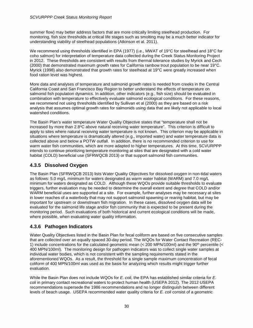
SCVURPPP Creek Status Monitoring Report
summer flow) may better address factors that are more critically limiting steelhead production. For monitoring, fish size thresholds at critical life stages such as smolting may be a much better indicator for understanding viability of steelhead populations (Atkinson et al. 2011).
We recommend using thresholds identified in EPA (1977) (i.e., MWAT of 19°C for steelhead and 18°C for coho salmon) for interpretation of temperature data collected during the Creek Status Monitoring Project in 2012. These thresholds are consistent with results from thermal tolerance studies by Myrick and Cech (2000) that demonstrated maximum growth rates for California rainbow trout population to be near 19°C. Myrick (1998) also demonstrated that growth rates for steelhead at 19°C were greatly increased when food ration level was highest.
More data and analyses of temperature and salmonid growth rates is needed from creeks in the Central California Coast and San Francisco Bay Region to better understand the effects of temperature on salmonid fish population dynamics. In addition, other indicators (e.g., fish size) should be evaluated in combination with temperature to effectively evaluate salmonid ecological conditions. For these reasons, we recommend not using thresholds identified by Sullivan et al (2000) as they are based on a risk analysis that assumes optimal growth rates for salmonids using data that are likely not applicable to local watershed conditions.
The Basin Plan’s water temperature Water Quality Objective states that “temperature shall not be increased by more than 2.8oC above natural receiving water temperature”. This criterion is difficult to apply to sites where natural receiving water temperature is not known. This criterion may be applicable in situations where temperature is dramatically altered (e.g., imported water) and water temperature data is collected above and below a POTW outfall. In addition, there is no recommended criterion to use for warm water fish communities, which are more adapted to higher temperatures. At this time, SCVURPPP intends to continue prioritizing temperature monitoring at sites that are designated with a cold water habitat (COLD) beneficial use (SFRWQCB 2013) or that support salmonid fish communities.
4.3.5 Dissolved Oxygen The Basin Plan (SFRWQCB 2013) lists Water Quality Objectives for dissolved oxygen in non-tidal waters as follows: 5.0 mg/L minimum for waters designated as warm water habitat (WARM) and 7.0 mg/L minimum for waters designated as COLD. Although these WQOs provide suitable thresholds to evaluate triggers, further evaluation may be needed to determine the overall extent and degree that COLD and/or WARM beneficial uses are supported at a site. For example, further analyses may be necessary at sites in lower reaches of a waterbody that may not support salmonid spawning or rearing habitat, but may be important for upstream or downstream fish migration. In these cases, dissolved oxygen data will be evaluated for the salmonid life stage and/or fish community that is expected to be present during the monitoring period. Such evaluations of both historical and current ecological conditions will be made, where possible, when evaluating water quality information.
4.3.6 Pathogen Indicators Water Quality Objectives listed in the Basin Plan for fecal coliform are based on five consecutive samples that are collected over an equally spaced 30-day period. The WQOs for Water Contact Recreation (REC-1) include concentrations for the calculated geometric mean (< 200 MPN/100ml) and the 90th percentile (< 400 MPN/100ml). The monitoring design for pathogen indicators was to collect single water samples at individual water bodies, which is not consistent with the sampling requirements stated in the aforementioned WQOs. As a result, the threshold for a single sample maximum concentration of fecal coliform of 400 MPN/100ml was used as the basis for analyzing which results might trigger further evaluation.
While the Basin Plan does not include WQOs for E. coli, the EPA has established similar criteria for E. coli in primary contact recreational waters to protect human health (USEPA 2012). The 2012 USEPA recommendations supersede the 1986 recommendations and no longer distinguish between different levels of beach usage. USEPA recommended water quality criteria for E. coli consist of a geometric
30

SCVURPPP Creek Status Monitoring Report
mean of 126 CFU/100ml for samples collected in any 30-day interval and a statistical threshold value (STV) of 410 CFU/100ml. The STV approximates the 90th percentile of data and is used as the basis for evaluating E. coli results which might trigger a monitoring project under MRP Provision C.8.d.i. evaluation criteria. In this evaluation, the Most Probable Number (MPN) of bacteria colonies given by the analytical method is compared directly with the Colony Forming Units (CFUs) of the USEPA recommendations.
Two important issues should be considered when evaluating bacterial indicator organisms: 1) there is an imperfect correlation between bacterial indicator organisms and pathogens of public health concern; and 2) the potential for human exposure to the water bodies of interest is uncertain. Water Quality Objectives and Criteria for pathogen indicators were derived from epidemiological studies of people recreating at bathing beaches that received bacteriological contamination via treated human wastewater. Therefore, applying these thresholds to data collected from creeks where exposure via recreation is infrequent and ingestion of the water is highly unlikely, is highly questionable. Additionally, sources of fecal indicators in the watershed are likely non-human given the understanding of watershed sources. Recent research indicates that the source of fecal contamination is critical to understanding the human health risk associated with recreational waters and that the risk in recreational waters varies with various fecal sources (USEPA 2012). Thus, comparison of fecal indicator results in Santa Clara Valley creeks to WQOs and criteria may not be appropriate and should be interpreted cautiously.
4.3.7 Quality Assurance/Quality Control Data quality assessment and quality control procedures are described in detail in the BASMAA RMC QAPP (BASMAA 2014a). They generally involve the following the steps described in the following paragraphs.
Data Quality Objectives (DQOs) were established to ensure that data collected are of adequate quality and sufficient for the intended uses. DQOs address both quantitative and qualitative assessment of the acceptability of data. The qualitative goals include representativeness and comparability. The quantitative goals include specifications for completeness, sensitivity (detection and quantization limits), precision, accuracy, and contamination. To ensure consistent and comparable field techniques, pre-survey field training and in-situ field assessments were conducted. Field training and inter-calibration exercises were conducted to ensure consistency and quality of CRAM and bioassessment data. Field audits by Water Board staff were conducted to evaluate field crews on proper use of bioassessment protocols.
Data were collected according to the procedures described in the relevant SOPs, including appropriate documentation of data sheets and samples, and sample handling and custody. Laboratories providing analytical support to the RMC were selected based on demonstrated capability to adhere to specified protocols. Standard methods for CRAM are included in Collins et al. (2008).
Duplicate samples were collected at 10% of the sites sampled to evaluate precision of field sampling methods. Ten percent of the total number of BMI samples collected was submitted to the California Department of Fish and Wildlife (CDFW) Aquatic Bioassessment Laboratory for independent assessment of taxonomic accuracy, enumeration of organisms and conformance to standard taxonomic level. All data were thoroughly reviewed for conformance with QAPP requirements and field procedures were reviewed for compliance with the methods specified in the relevant SOPs. Data quality was assessed and qualifiers were assigned as necessary in accordance with SWAMP requirements.
Following completion of the field and laboratory work, the field data sheets and laboratory reports were reviewed by the SCVURPPP Program Quality Assurance Officer, and compared against the methods and protocols specified in the SOPs and QAPP. The findings and results were evaluated against the relevant DQOs to provide the basis for an assessment of programmatic data quality. A summary of data quality steps associated with water quality measurements is shown in Table 4.3. The data quality assessment consisted of the following elements:
• Conformance with field and laboratory methods as specified in SOPs and QAPP, including sample collection and analytical methods, sample preservation, sample holding times, etc.
31

SCVURPPP Creek Status Monitoring Report
• Numbers of measurements/samples/analyses completed vs. planned, and identification of reasons for any missed samples.
• Temperature data was checked for accuracy by comparing measurements taken by HOBOs with NIST thermometer readings in room temperature water and ice water prior to deployment.
• General water quality data was checked for accuracy by comparing measurements taken before and after deployment with measurements taken in standard solutions to evaluate potential drift in readings.
• Quality assessment laboratory procedures for accuracy and precision (i.e., laboratory duplicates, laboratory blanks, laboratory control samples, and matrix spikes) were implemented, and data which did not mean DQOs were assigned the appropriate flag.
• Field crews participated in two inter-calibration exercises prior to field assessments and attended a debriefing meeting at the end of field assessments to assess consistency among RMC field crews.
Table 4.3. Data quality steps implemented for temperature and general water quality monitoring.
Step Temperature (HOBOs) General Water Quality (sondes) Pre-event calibration / accuracy check conducted X X Readiness review conducted X X Check field datasheets for completeness X X Post-deployment accuracy check conducted X X Post-sampling event report completed X X Post-event calibration conducted X X Data review – compare drift against SWAMP MQOs X Data review – check for outliers / out of water measurements X X
5.0 Results and Discussion In this section, following a brief statement of data quality, the biological data are evaluated to produce a preliminary condition assessment for aquatic life in SCVURPPP creeks. The physical, chemical, and toxicity monitoring data are then evaluated against the trigger criteria shown in Table 4.4 (Tables 8.1 and H-1 of the MRP) to provide a preliminary identification of potential stressors. Data evaluation and interpretation methods are described in Section 4.0. The results of the stressor assessment have been used to develop source identification projects.
5.1 Statement of Data Quality A comprehensive QA/QC program was implemented by SCVURPPP, covering all aspects of the probabilistic and targeted monitoring. In general, QA/QC procedures were implemented as specified in the RMC QAPP (BASMAA, 2014a), and monitoring was performed according to protocols specified in the RMC SOPs (BASMAA, 2014b), and in conformity with SWAMP protocols. Details of the results of evaluations of laboratory-generated QA/QC results are included in Attachment B. Issues noted by the laboratories and/or field crews are summarized below.
5.1.1 Bioassessment Prior to sampling in WY2014, field training and inter-calibration exercises with four other field crews were conducted to ensure consistency and quality of bioassessment data. While there are no quantitative
32

SCVURPPP Creek Status Monitoring Report
methods to assess quality assurance of physical habitat conditions, it was clear from the results that measurements taken by the SCVURPPP field crew rarely deviated from those of other crews.
The field crew was audited once during the field season by a representative of SWAMP to ensure consistency with SWAMP protocols. This audit is also intended to ensure consistency among RMC participants. Audits conducted by SWAMP did not result in any notable issues needing to be addressed regarding field procedures. Field sampling protocols, sample handling, documentation and packaging/delivery of samples were all executed properly as required by the QAPP and in accordance with the RMC SOPs. All field instruments were properly calibrated and cleaned within the necessary time restrictions.
Several biological assessment sites had to be sampled along a shortened reach (less than 150 m), and in some cases, stream characterization points may have been moved along the reach due to physical limitations or obstructions. Efforts were made to minimize the distance between the target collection location and the more accessible replacement location. Collection of algae samples was difficult at several sites due to varying levels of algal growth, making it challenging to collect a distinguishable clump for analysis.
Issues with the BMI laboratory analysis were noted, as follows:
• During BMI taxonomic QA analysis, one minor counting discrepancy and one minor taxonomic discrepancy were noted between the original BioAssessment Services results and the QA recount conducted by the CDFW Aquatic Bioassessment Laboratory. Menetus opercularis was identified by BioAssessment Services to the subfamily/tribe level (Menetus), but was identified to the species level by the CDFW Aquatic Bioassessment Laboratory. Additionally, the CDFW laboratory noted that a Tanytarsini larva was found in the Orthocladiinae vial and a Chironomini pupa was found with the Orthocladiinae pupae. Because Tanytarsini and Chironomini were both identified correctly in the sample, these likely represent oversights or sorting errors rather than true misidentifications.
• In accordance with the QAPP, BMIs were assessed to the Southwest Association of Freshwater Invertebrate Taxonomist (SAFIT) Standard Taxonomic Effort (STE) Level 1. BMIs from WY2014 will be re-analyzed to SAFIT STE Level 2 at a later date.
Issues with the algae laboratory analysis were noted, as follows:
• The only challenges to the qualitative macroalgae qualitative analysis were finding reproductive structures for species-level identification for Oedogonium and Spirogyra.
• Macroalgae was present in eight of the 22 total algae samples (20 samples and two duplicates). Those samples were subsequently analyzed for the presence of epiphytes.
• Detritus and lack of algae on the slides were the main issues with the microalgae samples. For more than half of the samples, the initially concentrated subsamples (from 10 ml to 1 ml) were diluted to 2, 3 or 5 ml, and 0.05 ml was placed on the slide to help disseminate the detritus and silt. Many samples were very sparse. Fewer than 20 algal counting entities were recorded in 8 samples. At least 150 algal (but less than 300) counting entities were recorded in 9 samples and 300 units were recorded in the remaining 5 samples.
• Similarly, for diatom analysis, the large amount of detritus made identification of the valves and capturing quality synoptic reference images somewhat difficult. Five taxa were not identified to species level. All samples reached the target 600-valve count.
• Five diatom and algae taxa found in SCVURPPP samples were not included in the existing SWAMP list of taxonomic identifications. The laboratory is working with SWAMP to reconcile the differences.
33

SCVURPPP Creek Status Monitoring Report
5.1.2 Nutrients and Conventional Analytes Caltest Laboratories analyzed all water chemistry samples for the SCVURPPP in WY2014. Caltest performed all internal QA/QC requirements as specified in the QAPP and reported their findings to the RMC. Key water chemistry Measurement Quality Objectives (MQOs) are listed in RMC QAPP Tables 26-1, 26-2, 26-5, and 26-7.
Several issues were noted with respect to water chemistry analyses, as follows:
• In past years, free chlorine measurements were sometimes greater than total chlorine residual measurements. As a result, the SCVURPPP field crew made sure that water for both tests was drawn from the same sample as opposed to drawing one sample after the other. The introduction of the HACH Pocket Colorimeter II in WY2014 as a replacement for the ChemMetrics test kits using in previous years improved the reliability of the chlorine readings. However, there was a learning curve associated with the new instrument and the following issues arose:
o Sample vials may have been over filled at the initial chlorine site, diluting the test reagent, leading to a lower chlorine reading. These data points have been flagged as questionable.
o The sample vials were found to have been stained over time from the test reagent, while the vial used to zero the instrument was still clear. As a result, some chlorine readings were very high. The field crew returned to sites with suspiciously high readings to resample chlorine, making sure to zero the instrument with the stained sample vial. The original readings were rejected and replaced with the new readings. As this issue was discovered early on, only three sites were resampled.
• A limited number of lab sample results for nutrients and conventional parameters were flagged due to minor QA/QC issues. These results were not thought to affect the validity of sample results and were not rejected. Included were the following:
o In one batch, low level contamination was measured in the chloride laboratory blank. Three samples were associated with this batch and their results were flagged, but not rejected. Laboratory personnel concluded that the lab blank contamination did not affect the sample results because only results above the Reporting Limit (RL) but less than 10 times the result in the blank would be considered invalid and rerun. As chloride results for the three samples in the batch were greater than 10 times the lab blank value, the results were considered valid.
o Several matrix spike (MS) and matrix spike duplicate (MSD) percent recoveries (PR) exceeded the MQO range listed in the RMC QAPP for various conventional analytes including chloride, dissolved organic carbon (DOC), nitrite, Total Kjeldahl Nitrogen (TKN), and silica. The affected samples have been assigned the appropriate flag.
• In accordance with the QAPP, field duplicates were collected at two (10%) of the 20 SCVURPPP sites sampled this year. Lab results of water chemistry field duplicate results are shown in Attachment B. The MQO for relative percent difference (RPD) was exceeded for three constituents (carbonate, Total Kjeldahl Nitrogen, and phosphorus) at the first site and three constituents (orthophosphate, chlorophyll a, and ash free dry mass) at the second site. With the exception of carbonate, these are the same constituents that have exceeded MQOs in prior years of sampling. Due to the nature of chlorophyll a and AFDM collection, discrepancies are to be expected due to the potential natural variability in algae production within the reach and the collection of field duplicates at different locations along each transect (as specified in the protocol). Discrepancies between other constituents are attributed to timing, i.e., not collecting the duplicate at the exact moment the original sample is collected. Field crews will continue to make an effort in subsequent years to collect the original and duplicate samples in an identical fashion.
34

SCVURPPP Creek Status Monitoring Report
• The QAPP requires field blanks to be collected and analyzed at a frequency of 5% of all samples collected for these parameters; this equates to a total of three such samples for the RMC total of 60 samples regionwide. The 5% requirement was exceeded in WY2014. Two were collected at SMCWPPP sites, two were collected at ACCWP sites, and two more were collected at CCCWP sites. Caltest analyzed these water chemistry field blank samples and detected no contaminants.
• Laboratory reports list the continuing calibration verification PR range as 85-115% or 90-110% for some conventional analytes (nutrients) while the RMC QAPP lists the PR as 80-120% for all conventional analytes in water.
5.1.3 Toxicity Two of the three aquatic toxicity samples collected during a storm in February 2014 (sites 205R00883 and 205R00979) were affected during testing by pathogen-related mortality (PRM), a fairly common cause of interference in aquatic sample toxicity tests with ambient surface waters. PRM was observed in one replicate for the first site and in two test replicates for the second site. The EPA testing manual indicates that a coefficient of variation (CV) greater than 40% may be indication of pathogen interference; however, there is no mandate that the CV must be greater than 40%. For site 205R00883, the survival CV was 12.4% and the growth CV was 4.3%. For site 205R00979, the survival CV was 6.1% and the growth CV was 5.0%. Although the test CVs were not greater than 40% for these samples, it was clear from the photographs provided by the laboratory that PRM was present. As PRM was not observed in the Laboratory Control treatment, the laboratory concluded that the PRM was not related to the source of the test organisms or laboratory practices. Because no toxicity to Pimephales promelas (i.e., fathead minnow) was observed in these samples, PRM protocols were not pursued.
5.1.4 Sediment Chemistry Caltest Laboratories performed all sediment chemistry analyses for SCVURPPP, with the exception of the grain size distribution and total organic carbon (TOC) analyses, which were sub-contracted by Caltest to Soil Control Laboratories. Caltest conducted all QA/QC requirements as specified in the RMC QAPP and reported their findings to the RMC. Key sediment chemistry MQOs are listed in RMC QAPP Tables 26-4, 26-6, and 26-7. Several issues were reported by the analytical laboratory (Caltest), and the sediment chemistry data were qualified accordingly. These issues included the following:
• The continuing calibration verification (laboratory control sample) percent recovery for zinc and three PAHs (benz(a)anthracene, benzo(a)pyrene, perylene) slightly exceeded the MQO range specified by the RMC QAPP for synthetic organic compounds.
• The MSD relative percent difference (RPD) exceeded the RMC QAPP MQOs for two organochlorides (DDT (p,p’) and endrin) and several PAHs (benz(a)anthracene, benzo(b)fluoranthene, benzo(a)pyrene, benzo(e)pyrene, benzo(g,h,i)perylene, chrysene, fluoranthene, and pyrene).
In addition, the following issues with sediment chemistry were noted in WY2014:
• The RMC QAPP lists the maximum RPD for inorganic analytes (metals) as 25%, while the laboratory report lists the maximum as 30% for most metals and 35% for mercury.
• The maximum RPD for synthetic organics listed in the sediment laboratory report lists ranges from 30 to 50% for most analytes, and are much higher for gamma-BHC (Lindane) and p,p'-DDT at 52% and 59%,respectively. However, the RMC QAPP lists the MQO as less than 25% RPD for all synthetic organics.
• These discrepancies in maximum RPD resulted in several analytes not being flagged in laboratory reports when they should have been. These were flagged by the program in data submittals. All other analyte groups (metals, pyrethroids, etc.) had relatively low RPDs.
35

SCVURPPP Creek Status Monitoring Report
The RMC QAPP requires collection and analysis of duplicate sediment samples at a rate of 10% of total samples collected. For WY2014, SMCWPPP collected one sediment sample field duplicate to account for the 10 sediment sites monitored by the RMC in 2014. The sediment sample and field duplicate were collected together using the Sediment Scoop Method described in the RMC SOP, homogenized, and then distributed to two separate containers. Of the 70 constituents analyzed, 96%, or 67, of those constituents met the RPD MQO listed in the RMC QAPP for the sediment chemistry field duplicate sample. Only cis-permethrin and three particle size results (granule, coarse clay, and medium clay) exceeded the RPD MQO of 25%.
Lab results of the sediment chemistry field duplicates are shown in Attachment B. [Note that because of the variability in reporting limits, values less than the Reporting Limit (RL) were not evaluated for sediment RPDs.] That RPDs fall outside of control limits for field duplicates should not be surprising in that the control limits associated with SWAMP comparable programs are identical between lab duplicates and field duplicates, even though sources of variability are much larger associated with field duplicates. 5.1.5 Targeted Monitoring Field data sheets and laboratory reports were reviewed by the local Program Quality Assurance Officer, and the results evaluated against the relevant MQOs. Results were compiled for the qualitative metrics (representativeness and comparability), as well as the quantitative metrics (completeness, precision, accuracy). The following summarizes the results of the data quality assessment:
• Temperature data (from HOBOs) was collected at 10 targeted site locations in 2014, a small increase over the required 8 locations, and insurance in the event that field equipment is lost or damaged or that streams dried up prior to the end of the sampling period. As a result, over 100% of the expected data was captured.
• Continuous water quality data (temperature, pH, dissolved oxygen, specific conductivity) was collected at three sites during two two-week periods in the spring and summer resulting in over 100% of the expected data results.
• Continuous water quality data met measurement quality objectives (accuracy) for all parameters and are included in Table 5.1.
• Two laboratory duplicates were run on ACCWP and CCCWP pathogen indicator samples. The RPDs for E.coli exceeded the target ranges specified in the RMC QAPP, but only one RPD for fecal coliform exceeded the MQO. Given the nature of pathogen indicator sampling, these results are not surprising.
• .
• No contamination was detected in pathogen laboratory blanks.
Table 5.1. Dissolved oxygen, pH and specific conductivity drift over two two-week monitoring events in WY2014.
Parameter Measurement
Quality Objectives
205STE065 205STE071 205STE105
Event 1 Event 2 Event 1 Event 2 Event 1 Event 2
Dissolved Oxygen (mg/l) ± 0.5 mg/L or 10% 0.23 -0.15 -0.2 0.7% -0.06 0.07
pH 7.0 ± 0.2 0.07 -0.1 0.06 0.14 -0.01 -0.05
pH 10.0 ± 0.2 0.06 0.1 0 0.15 0.02 -0.04
Specific Conductance (uS/cm) ± 10% 0.3% -0.3% -0.1% 0.1% 0.6% 0.2%
36

SCVURPPP Creek Status Monitoring Report
5.2 Condition Assessment This section addresses the core management question “Are conditions in local receiving water supportive of or likely supportive of beneficial uses?” or more specifically, “What is the condition of aquatic life in creeks in Santa Clara County?” The RMC probabilistic monitoring design provides an unbiased framework for data evaluation that, with adequate sample size (n=30), will allow a condition assessment of ambient aquatic life within known estimates of precision. Over 30 samples have been collected and analyzed in Santa Clara County; however, this report only evaluates the 20 sites sampled in WY2014 and therefore, a full condition assessment was not conducted for this report. Although the data set is not yet sufficient to develop statistically representative conclusions addressing the second core management question (“To what extent does the condition of aquatic life in urban and non-urban creeks differ in Santa Clara County?”), comparisons are made between the two types of sites. At least 30 samples from each creek type (urban and non-urban) would be required for statistically representative conclusions. 5.2.1 Benthic Macroinvertebrates Biological condition, presented as CSCI score, for the 20 probabilistic sites sampled in Santa Clara County during WY2014 are listed in Table 5.2 and illustrated in Figure 5.1. The range of CSCI scores is 0.32 to 1.28, with a median score of 0.61. Site characteristics related to land use classification, flow status15, and channel modification status16 are presented in the table for reference. Using the condition categories for CSCI presented in this report, four sites (20%) scored as “likely intact,” four sites (20%) scored as “possibly intact,” one site (5%) scored as “likely altered,” and eleven sites (55%) scored as “very likely altered” (Table 5.6). The sites rated as “likely intact” included all three non-urban sites with perennial flow and one “urban” site17 (1299) located on Arroyo Aguague in an undeveloped portion of Alum Rock Park. The four sites rated as possibly intact were all urban and perennial. One of the “urban” sites (1098) was located on Guadalupe Creek at the edge of Mid-Peninsula Regional Open Space District land in a concrete channel just upstream of a fish ladder. The remaining twelve sites rated as likely or very likely altered were all urban, with the exception of the site on Limekiln Creek (266) which was classified as non-urban, but located downstream of a rock quarry (Table 5.6). Three of the twelve sites were classified as highly modified channels.
15 Flow status was based on visual observations at each site made during fall season of 2013 or 2014. 16 Highly modified channels were defined as having armored bed and banks (e.g., concrete, gabion, rip rap) for majority of the reach or characterized as highly channelized earthen levee. 17 Some sites classified as “urban” are actually located in less- or undeveloped areas due to assumptions inherent in the probabilistic monitoring design.
37

SCVURPPP Creek Status Monitoring Report
Table 5.2. CSCI scores and condition categories for probabilistic sites sampled in WY2014 (n=20). Condition categories developed by Mazor et al. (in review) are shown for each site.
Station Code Creek Land
Use1 Modified Channel Flow2
CSCI
Score Condition Category
205R00330 Hick's Creek NU N P 1.28 Likely Intact 205R00394 Austrian Gulch NU N P 1.25 Likely Intact 205R00362 Lyndon Canyon NU N P 1.10 Likely Intact 205R01299 Arroyo Aguague U N NP 0.95 Likely Intact 205R01098 Guadalupe Creek U Y P 0.92 Possibly Intact 205R01434 Arroyo Calero U N P 0.82 Possibly Intact 205R00938 San Tomas Aquino Creek U N P 0.81 Possibly Intact 205R00883 Adobe Creek U N P 0.80 Possibly Intact 205R01443 Stevens Creek U N P 0.72 Likely Altered 205R01539 Los Gatos Creek U N P 0.61 Very Likely Altered 205R01226 Los Gatos Creek U N P 0.59 Very Likely Altered 205R01187 Stevens Creek U N P 0.58 Very Likely Altered 205R00266 Limekiln Creek NU N NP 0.57 Very Likely Altered 205R00851 Los Coches Creek U N NP 0.55 Very Likely Altered 205R01578 San Tomas Aquino Creek U N NP 0.55 Very Likely Altered 205R01027 Guadalupe River U N P 0.50 Very Likely Altered 205R00979 Lower Silver Creek U Y P 0.49 Very Likely Altered 205R01306 Ross Creek U Y P 0.46 Very Likely Altered 205R00915 Thompson Creek U N P 0.46 Very Likely Altered 205R01091 Saratoga Creek U Y P 0.32 Very Likely Altered
1 NU = non-urban, U = urban (as classified by the GIS-based probabilistic monitoring design) 2 P = perennial, NP = non-perennial
38

SCVURPPP Creek Status Monitoring Report
Figure 5.1. Location and CSCI condition category for 20 probabilistic sites sampled in WY2014, Santa Clara County.
39

SCVURPPP Creek Status Monitoring Report
Table 5.2 lists the land use (urban or non-urban) and flow class (perennial or non-perennial) for each probabilistic site. There was very little difference in CSCI scores between perennial (n=16) and non-perennial (n=4) sites (Figure 5.2). The CSCI scores were generally lower for sites classified as urban18 compared to non-urban sites (Figure 5.3).
Figure 5.2. Box plots showing distribution of CSCI scores for perennial (n=16) and non-perennial (n=4) sites sampled in Santa Clara County in WY2014.
Figure 5.3. Box plots showing distribution of CSCI scores for urban (n=16) and non-urban (n=4) sites sampled in Santa Clara County in 2014.
18 The land use classification is based on the RMC sample frame, which was developed using a combination of urban areas (as defined by Association of Bay Area Governments) and city boundaries. For some areas, city boundaries include parks and undeveloped areas. Thus sampling locations that are classified as urban may have a wide range of impacts associated with urban development.
Non-perennial (n=4) Perennial (n=16)
CSCI
Sco
re
0.00
0.25
0.50
0.75
1.00
1.25
1.50
Nonurban (n=4) Urban (n=16)
CSCI
Sco
re
0.00
0.25
0.50
0.75
1.00
1.25
1.50
40

SCVURPPP Creek Status Monitoring Report
The amount (i.e., percent) of impervious area within the upstream watershed for each sampling location was calculated using existing land use data in GIS. Impervious coefficients for land use classes were derived from SMCWPPP (2000). Three classes of imperviousness (<3%, 3-10%, and > 10%) were used to define the range of potential stress to biological condition at each sample location. The distribution of CSCI scores for the three categories of imperviousness is shown in Figure 5.4. As expected, CSCI scores were lowest for the sites with the most imperviousness. However, there is little difference between the sites with the least imperviousness and sites in the middle class. The lack of differentiation may be due to the small sample size in WY2014, especially in the 3-10% imperviousness class.
Figure 5.4. Box plots showing distribution of CSCI scores at sites sampled in Santa Clara County in WY2014 for three classifications of % watershed imperviousness.
5.2.2 Algae Biological condition, presented as “H20” hybrid IBI (Algae IBI) scores for the 20 probabilistic sites sampled in Santa Clara County during WY2014 are listed in Table 5.3. The Algae IBI scores across all the sites ranged from 11 to 80. Algae IBI scores ranged from 66 to 80 at non-urban sites and 11 to 68 at urban sites. The highest IBI scores all occurred at non-urban sites. The Algae IBI scores were moderately correlated with CSCI scores (r2 = 0.316, p = 0.01) (Figure 5.5). These results suggest that different stressors impact the algae assemblage as compared to the BMI assemblage.
Watershed Percent Imperviousness
<3% (n=9) 3-10% (n=3) >10% (n=8)
CSCI
Sco
re
0.00
0.25
0.50
0.75
1.00
1.25
1.50
41

SCVURPPP Creek Status Monitoring Report
Table 5.3. Algae IBI scores for 20 probabilistic sites sampled in Santa Clara County during WY2014.
StationCode Creek Land Use1
Modified Channel Flow2
Hybrid “H20” IBI
Score 205R00266 Limekiln Creek NU N NP 80 205R00362 Lyndon Canyon NU N P 70 205R00330 Hick's Creek NU N P 68 205R01299 Arroyo Aguague U N NP 68 205R00394 Austrian Gulch NU N P 66 205R00851 Los Coches Creek U N NP 59 205R01578 San Tomas Aquino Creek U N NP 55 205R01434 Arroyo Calero U N P 50 205R01539 Los Gatos Creek U N P 49 205R01226 Los Gatos Creek U N P 48 205R01443 Stevens Creek U N P 48 205R00938 San Tomas Aquino Creek U N P 44 205R01098 Guadalupe Creek U Y P 44 205R01091 Saratoga Creek U Y P 42 205R01306 Ross Creek U Y P 32 205R00883 Adobe Creek U N P 31 205R01027 Guadalupe River U N P 31 205R01187 Stevens Creek U N P 29 205R00915 Thompson Creek U N P 21 205R00979 Lower Silver Creek U Y P 11
1 NU = non-urban, U = urban (as classified by the GIS-based probabilistic monitoring design) 2 P = perennial, NP = non-perennial
Figure 5.5. Linear regression of Algae IBI score (H2)) and CSCI score for 20 probabilistic sites in Santa Clara County sampled during WY2014 (r2 = 0.316, p = 0.01).
CSCI Score
0.2 0.4 0.6 0.8 1.0 1.2 1.4
H20 S
core
0
20
40
60
80
100
r2 = 0.316
42

SCVURPPP Creek Status Monitoring Report
In contrast to the CSCI scores where there was very little difference between non-perennial and perennial streams, the non-perennial sites generally had higher Algae IBI scores compared to the perennial sites (Figure 5.6). The Algae IBI scores had similar pattern to CSCI scores for three disturbance classes, based on percent impervious area, with limited overlap in scores between the high and low disturbance/imperviousness classes (Figure 5.7).
Figure 5.6. Box plots showing distribution of H20 IBI scores for perennial (n=16) and non-perennial (n=4) sites sampled in Santa Clara County in 2014.
Figure 5.7. Box plots showing distribution of H20 IBI scores at sites sampled in Santa Clara County in 2014 for three classifications of % watershed imperviousness.
Non-perennial (n=4) Perennial (n=16)
H20
Sco
re
0
10
20
30
40
50
60
70
80
90
100
Watershed Percent Imperviousness
<3% (n=9) 3-10% (n=3) >10% (n=8)
H20
Sco
re
0
10
20
30
40
50
60
70
80
90
100
43

SCVURPPP Creek Status Monitoring Report
5.3 Physical Habitat Condition Individual attribute and total scores for PHAB and CRAM are listed in Table 5.4. Total PHAB scores ranged from 5 to 55 and CRAM scores ranged from 41 to 88. The majority of sites with higher total PHAB scores were non-urban. Sites with highest total CRAM scores were both urban and non-urban. Total PHAB scores and total CRAM scores were correlated ((r2 = 0.660, p.< 0.01).) (Figure 5.8). Comparison between CSCI scores and total PHAB scores for 20 probabilistic sites are shown in Figure 5.9. There was moderate correlation between PHAB score and CSCI score (r2 = 0.398, p = 003). The Algae IBI scores and total PHAB scores were also moderately correlated (r2 = 0.471, p < 0.001) (Figure 5.10). There was minimal correlation between CRAM scores and CSCI or Algae IBI scores. Physical habitat endpoints and urban land use characteristics for the 20 probabilistic sites are listed in Table 5.5. These stressor variables are compared to biological condition scores in Section 5.4.
Figure 5.8. Total CRAM scores and Total PHAB scores are compared for all probabilistic sites (r2 = 0.660, p.< 0.01).
PHab Score
0 10 20 30 40 50 60
CRAM
Sco
re
30
40
50
60
70
80
90
100
r2 = 0.660
44

SCVURPPP Creek Status Monitoring Report
Figure 5.9. CSCI scores and Total PHAB scores are compared for all probabilistic sites (r2 = 0.398, p = 0.003).
Figure 5.10. Algal IBI scores and Total PHAB scores are compared for all probabilistic sites (r2 = 0.471, p < 0.001).
PHab Score
0 10 20 30 40 50 60
CSCI
Sco
re
0.2
0.4
0.6
0.8
1.0
1.2
1.4
r2 = 0.398
PHab Score
0 10 20 30 40 50 60
H20
Scor
e
0
20
40
60
80
100
r2 = 0.471
45

SCVURPPP Creek Status Monitoring Report
Table 5.4. PHAB and CRAM assessment scores at 20 probabilistic sites in Santa Clara County for WY2014.
Station Code Creek Name Land
Use
PHAB CRAM
Channel Alteration
Epifaunal Substrate
Sediment Deposition
Total Score Land Hydro Physical Biotic Total
Score
205R00362 Lyndon Canyon NU 20 19 16 55 56 100 75 67 74 205R01299 Arroyo Aguague U 20 18 13 51 100 83 75 64 81 205R00394 Austrian Gulch NU 20 18 11 49 63 83 75 75 74 205R00330 Hick's Creek NU 15 16 15 46 56 83 75 81 74 205R00266 Limekiln Creek NU 16 14 15 45 90 92 88 81 88 205R01226 Los Gatos Creek U 10 12 14 36 66 58 63 75 66 205R01434 Arroyo Calero U 15 14 6 35 80 75 75 75 76 205R01187 Stevens Creek U 19 12 1 32 53 75 88 75 73 205R01578 San Tomas Aquino Creek U 10 10 12 32 63 67 88 78 74 205R01443 Stevens Creek U 15 12 4 31 50 58 63 81 63 205R00938 San Tomas Aquino Creek U 8 12 10 30 41 58 75 78 63 205R01027 Guadalupe River U 10 10 10 30 38 83 88 67 69 205R00883 Adobe Creek U 16 8 5 29 80 42 50 75 62 205R01539 Los Gatos Creek U 10 10 8 28 55 75 75 67 68 205R00851 Los Coches Creek U 10 7 5 22 36 92 75 64 67 205R00979 Lower Silver Creek U 4 2 16 22 50 83 38 56 57 205R00915 Thompson Creek U 9 4 3 16 68 50 63 64 61 205R01091 Saratoga Creek U 9 3 2 14 63 58 50 69 60 205R01098 Guadalupe Creek U 2 2 2 6 73 42 50 75 60 205R01306 Ross Creek U 2 2 1 5 29 58 38 39 41
46

SCVURPPP Creek Status Monitoring Report
Table 5.5. Physical habitat condition scores and endpoints calculated from habitat measurements conducted during bioassessments in WY2014.
Station Code Creek Name Land Use % Algae Cover % Canopy Cover
% Sands & Fines
HDI Score
% Urban % Impervious
205R00266 Limekiln Creek NU 17.1 97.3 2.9 0.8 2.9% 1.5% 205R00330 Hick's Creek NU 21.4 89.4 1.0 0.6 0.0% 1.0% 205R00362 Lyndon Canyon NU 15.0 99.3 6.7 0.1 2.6% 3.4% 205R00394 Austrian Gulch NU 15.3 98.5 9.5 0.7 0.0% 1.0% 205R00851 Los Coches Creek U 22.2 94.9 61.0 1.7 14.8% 1.6% 205R00883 Adobe Creek U 25.6 97.3 30.5 1.6 33.8% 7.9% 205R00915 Thompson Creek U 24.0 73.0 25.7 2.0 32.9% 15.7% 205R00938 San Tomas Aquino Creek U 18.9 94.4 30.8 1.8 52.8% 10.6% 205R00979 Lower Silver Creek U 32.2 17.9 6.7 2.2 50.3% 23.8% 205R01027 Guadalupe River U 20.2 66.6 45.7 1.5 46.1% 24.4% 205R01091 Saratoga Creek U 38.8 29.0 33.3 2.2 48.9% 25.2% 205R01098 Guadalupe Creek U 22.0 92.0 20.0 1.3 0.1% 1.0% 205R01187 Stevens Creek U 20.0 96.5 37.1 0.7 3.7% 1.7% 205R01226 Los Gatos Creek U 32.9 70.3 34.3 2.6 24.5% 12.3% 205R01299 Arroyo Aguague U 24.6 85.7 5.7 0.2 0.7% 1.3% 205R01306 Ross Creek U 39.8 5.9 21.9 2.0 81.4% 30.9% 205R01434 Arroyo Calero U 25.8 93.7 30.5 0.9 11.6% 2.7% 205R01443 Stevens Creek U 29.1 98.8 40.0 2.0 6.0% 2.4% 205R01539 Los Gatos Creek U 26.0 89.7 17.1 2.2 31.2% 16.7% 205R01578 San Tomas Aquino Creek U 24.3 94.4 16.3 1.5 27.0% 5.3%
47

SCVURPPP Creek Status Monitoring Report
5.4 Stressor/WQO Assessment This section addresses the core management question “Are water quality objects, both numeric and narrative, being met in local receiving waters, including creeks, rivers, and tributaries?” or more specifically, “What are the major stressors to aquatic life in Santa Clara County?” Potential stressors to aquatic life (such as PHAB measures, percent impervious, and water quality) were compared to biological condition scores to evaluate their importance as major stressors to aquatic life. In addition, each monitoring category required by MRP Provision C.8.c, Table 8.1 is associated with a specification for “Results that Trigger a Monitoring Project in Provision C.8.d.i” (Stressor/Source Identification). The definitions of these “Results that Trigger…”, as shown in Table 8.1, are considered to represent “trigger criteria”, meaning that the relevant monitoring results should be forwarded for consideration as potential Stressor/Source Identification Projects per Provision C.8.d.i. The trigger criteria/thresholds are listed in Table 4.4 of this report. The physical, chemical, and toxicity monitoring data collected during WY2014 were evaluated against the trigger criteria. When the data analysis indicated that the associated trigger criteria were met, those sites and results were identified as potentially warranting further investigation.
5.4.1 Potential Stressors to Biological Condition Physical habitat, general water quality, and water chemistry (e.g., nutrients) data were evaluated as potential stressors to biological condition. These data were collected synoptically with biological data during bioassessments at probabilistic sites during WY2014. Using the Sigma Plot statistical software platform, the variables were tested for normality using the Shapiro-Wilk Test. Several environmental parameters were not normally distributed. Correlations between biological assessment tools and environmental variables were evaluated using the Spearman rank method. Coefficients values greater than ±0.7 indicate a strong relationship between variables. If the p-value is ≤0.05, the correlation is considered statistically significant.
Statistically significant variables with the highest correlations are indicated as shaded cells in Table 5.6. There are slightly more significant variables explaining Algae IBI scores (epifaunal substrate score, CRAM score, unionized ammonia, and Total Kjeldahl Nitrogen) compared to CSCI scores (epifaunal substrate score, percent impervious, and chloride). Epifuanal substratre was the only environmental variable that had strong relationship with both biological assessment scores.
48

SCVURPPP Creek Status Monitoring Report
Table 5.6. Spearman Rank Correlations for biological condition scores (CSCI and algae H20 IBI) and environmental variables. Coefficients greater than + 0.7 are indicated as shaded cells.
Independent Variables Shapiro-Wilk CSCI H20
Normal Distribut
ion p-value
Spearman Rank
Correlation p-value
Spearman Rank
Correlation p-value
Biological Assessment Tool
CSCI Yes 0.08 0.58 0.01 Algae H20 IBI Yes 0.89 0.58 0.01
Potential Stressor
HDI Score Yes 0.34 -0.63 < 0.01 -0.55 0.01 Algae Cover Yes 0.18 -0.48 0.03 -0.39 0.09 Canopy Cover No < 0.01 0.54 0.01 0.47 0.04 Sands & Fines Yes 0.48 -0.40 0.08 -0.48 0.03 Channel Alteration (PHAB) Yes 0.11 0.58 0.01 0.56 0.01 Epifaunal Substrate (PHAB) Yes 0.16 0.72 < 0.01 0.72 < 0.01 Sediment Deposition (PHAB) Yes 0.06 0.46 0.04 0.53 0.02 CRAM Total Score Yes 0.42 0.52 0.02 0.76 < 0.01 Biotic Structure (CRAM) No < 0.01 0.44 0.05 0.35 0.13 Buffer and Landscape (CRAM) Yes 0.91 0.34 0.11 0.30 0.19 Hydrology (CRAM) Yes 0.23 0.19 0.41 0.59 0.01 Physical Structure (CRAM) No 0.02 0.21 0.36 0.46 0.04 % Impervious Watershed Area No < 0.01 -0.72 < 0.01 -0.61 < 0.01 Chloride No < 0.01 -0.75 < 0.01 -0.60 < 0.01 Unionized Ammonia No < 0.01 -0.56 0.01 -0.80 < 0.01 Nitrate as N No < 0.01 -0.20 0.40 -0.61 < 0.01 Nitrogen, Total Kjeldahl Yes 0.862 -0.46 0.04 -0.75 < 0.01 Suspended Sediment Concentration No < 0.01 -0.51 0.02 -0.66 < 0.01 Specific Conductivity Yes 0.551 -0.26 0.26 -0.19 0.42 Temperature Yes 0.474 -0.45 0.04 -0.55 0.01
49

SCVURPPP Creek Status Monitoring Report
5.4.2 Nutrients and Conventional Analytes Descriptive statistics for nutrient and conventional analyte concentrations measured in samples collected synoptically during bioassessments are listed in Table 5.7. Chlorophyll α and ash free dry mass were measured in µg/L and mg/L, respectively, and were converted to volume per area units using a module developed by EOA. Trigger thresholds for chloride, unionized ammonia, and nitrate are shown in Table 5.7 for reference. No samples exceeded the thresholds.
Table 5.7. Descriptive statists for water chemistry results in Santa Clara County during WY2014.
Nutrients and Conventional Analytes Units N N ≥ RL Min Max Mean1 Median1
Trigger
Threshold Exceedance
Alkalinity (as CaCO3) (mg/L) 20 20 141 453 264.3 237 -- -- Ash Free Dry Mass (g/m2) 20 19 3.6 1387 277 118 -- -- Chloride (mg/L) 20 20 5.3 340 65.2 41.5 230/2502 5% Chlorophyll α (mg/m2) 20 18 14 155.8 57 47.8 -- -- Dissolved Organic Carbon (mg/L) 20 20 0.57 4.1 2.15 1.7 -- -- Ammonia (as N) (mg/L) 20 2 < 0.04 0.19 0.05 0.02 -- -- Unionized Ammonia (as N)3 (µg/L) 20 2 <0.03 3.23 0.85 0.45 25 0%
Nitrate (as N) (mg/L) 20 13 < 0.01 2.9 0.54 0.11 10 0% Nitrite (as N) (mg/L) 20 1 < 0.005 0.05 0.006 0 -- -- Total Kjeldahl Nitrogen (as N) (mg/L) 20 19 < 0.07 0.97 0.44 0.46 -- --
OrthoPhosphate (as P) (mg/L) 20 17 < 0.006 0.2 0.06 0.03 -- -- Phosphorus (as P) (mg/L) 20 18 < 0.007 0.2 0.07 0.05 -- -- Suspended Sediment Concentration (mg/L) 20 4 < 2 16 3.39 1 -- --
Silica (as SiO2) (mg/L) 20 20 11 38 19.85 19 -- -- 1 Mean and median concentrations calculated using ½ the method detection limit (MDL) for samples below the detection limit (ND). 2 The nitrate and 250 mg/L chloride thresholds apply to Title 22 drinking waters and sites with MUN beneficial use only. 3 Unionized ammonia estimated from ammonia, pH, temperature, and specific conductance per Emerson et al., 1975.
50

SCVURPPP Creek Status Monitoring Report
5.4.3 Chlorine Field testing for free chlorine and total chlorine residual was conducted at all probabilistic sites concurrent with spring bioassessment sampling and at a subset of the sites concurrent with dry season toxicity sampling. Chlorine concentrations and comparisons to the MRP Table 8.1 trigger threshold are listed in Table 5.8. The MRP trigger criterion for chlorine states, “After immediate resampling, concentrations remain >0.08 mg/L”. If a repeat chlorine measurement was not conducted, the original measurement was evaluated. Twenty-three measurements were collected in WY2014; 13% exceeded the threshold for free chlorine, and 22% exceeded the threshold for total chlorine residual. Lower Silver Creek (205R00979) exceeded the threshold for both free and total chlorine on both measurement dates. All four sites that exceeded chlorine thresholds were highly urban sites.
Table 5.8. SCVURPPP chlorine testing results compared to MRP trigger criteria for WY2014. Samples were taken twice at some sites when results exceeded 0.08 mg/L trigger. Values above the trigger are indicated by shaded cells.
Station Code Date Creek
Free Chlorine (mg/L)1, 2
Total Chlorine Residual (mg/L)1, 2
Exceeds Trigger? 3
(0.08 mg/L) 205R00266 4/23/2014 Limekiln Creek 0.04 0.05 No 205R00330 5/16/2014 Hick's Creek < 0.02 0.02 No 205R00362 5/22/2014 Lyndon Canyon < 0.02 < 0.02 No 205R00394 5/12/2014 Austrian Gulch < 0.02 0.02 No 205R00851 4/21/2014 Los Coches Creek < 0.024 < 0.024 No 205R00883 5/13/2014 Adobe Creek 0.04 0.06 No 205R00883 6/4/2014 Adobe Creek 0.03 0.03 No 205R00915 4/24/2014 Thompson Creek < 0.02 0.03 No 205R00938 4/30/2014 San Tomas Aquino Creek 0.02 0.03 No 205R00938 6/4/2014 San Tomas Aquino Creek 0.02 0.03 No 205R00979 4/24/2014 Lower Silver Creek 0.09 / 0.09 0.12 / 0.12 Yes 205R00979 6/4/2014 Lower Silver Creek 0.185 0.135 Yes 205R01027 5/5/2014 Guadalupe River 0.03 0.03 No 205R01091 5/5/2014 Saratoga Creek 0.03 / 0.04 0.08 / 0.09 Yes 205R01098 5/16/2014 Guadalupe Creek 0.04 0.05 No 205R01187 5/14/2014 Stevens Creek 0.10 / 0.09 0.13 / 0.13 Yes 205R01226 5/20/2014 Los Gatos Creek 0.02 0.02 No 205R01299 5/15/2014 Arroyo Aguague 0.05 / <0.02 0.04 No 205R01306 4/23/2014 Ross Creek 0.08 0.095 Yes 205R01434 5/21/2014 Arroyo Calero 0.02 0.02 No 205R01443 5/14/2014 Stevens Creek < 0.02 0.15 / 0.03 No 205R01539 5/20/2014 Los Gatos Creek 0.02 0.02 No 205R01578 4/22/2014 San Tomas Aquino Creek < 0.024 < 0.024 No
Number of samples exceeding 0.08 mg/L: 3 5 -- Percentage of samples exceeding 0.08 mg/L: 13% 22% -- 1 The method detection limit for the test kits is 0.02 mg/L. 2 Original and repeat samples are reported where conducted. The first value is the original sample, and the second value is the duplicate sample. 3 The trigger applies to both free and total chlorine measurements. 4 Questionable results – diluted test reagent. 5 Immediate resampling was not conducted at these sites.
51

SCVURPPP Creek Status Monitoring Report
5.4.4 Water and Sediment Toxicity Water toxicity samples were collected from a subset of urban probabilistic sites twice per year, during storm events and summer dry conditions. Samples were tested for toxic effects using four species: an algae (Selenastrum capricornutum), two aquatic invertebrates (Ceriodaphnia dubia and Hyalella azteca), and one fish species (Pimephales promelas or fathead minnow). Both acute and chronic endpoints (survival and reproduction/growth) were analyzed for Ceriodaphnia dubia and fathead minnow. Selenastrum capricornutum are tested only for the chronic (growth) endpoint and Hyalella azteca are tested only for the acute (survival) endpoint.
Table 5.9 provides a summary of toxicity testing results for water samples. One water sample was found to be toxic to Hyalella Azteca – the wet season sample from Lower Silver Creek. This sample did not meet the trigger criteria of being less than 50 percent of the control (see Table 5.11). Three samples were found to be chronically toxic to Ceriodaphnia dubia (San Tomas Aquino in both the wet and dry season, and Adobe Creek in the dry season); however, these results did not meet the trigger criteria (see Table 5.12).
Table 5.9. Summary of SCVURPPP water toxicity results for WY2014.
SCVURPPP Water Samples Test
Initiation Date
Toxicity relative to the Lab Control treatment?
Sample Station Creek Sample
Date Selenastrum
capricornutum Ceriodaphnia dubia Hyalella azteca Fathead Minnow
Growth Survival Reproduction Survival Survival Growth 205R00883 Adobe Creek 2/26/14 2/27/14 No No No No No No
205R00938 San Tomas Aquino Creek 2/26/14 2/27/14 No No Yes No No No
205R00979 Lower Silver Creek 2/26/14 2/27/14 No No No Yes No No
205R00883 Adobe Creek 6/4/14 6/5/14 No No Yes No No No
205R00938 San Tomas Aquino Creek
6/4/14 6/5/14 No No Yes No No No
205R00979 Lower Silver Creek
6/4/14 6/5/14 No No No No No No
During the dry season, sediment samples were collected at the same sites and tested for sediment toxicity and an extensive suite of sediment chemistry constituents. Sediment toxicity testing was performed with just one species, Hyalella azteca, a common benthic invertebrate. Both acute and chronic endpoints (survival and growth) were analyzed. Table 5.10 provides a summary of toxicity testing results for sediment samples. One sediment sample collected at site in Adobe Creek was determined to be acutely toxic. No chronic endpoint results indicated chronic toxicity at any site.
Table 5.10. Summary of SCVURPPP dry season sediment toxicity results for WY2014.
Dry Season Sediment Samples Date of
Analysis
Toxicity relative to the Lab Control treatment? Sample Station Creek Collection
Date Hyalella azteca
Survival Growth 205R00883 Adobe Creek 6/4/14 6/9/14 Yes No
205R00938 San Tomas Aquino Creek 6/4/14 6/9/14 No No
205R00979 Lower Silver Creek 6/4/14 6/9/14 No No
52
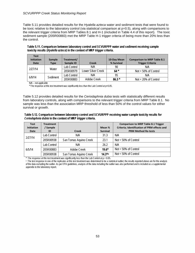
SCVURPPP Creek Status Monitoring Report
Table 5.11 provides detailed results for the Hyalella azteca water and sediment tests that were found to be toxic relative to the laboratory control (via statistical comparison at p=0.5), along with comparisons to the relevant trigger criteria from MRP Tables 8.1 and H-1 (included in Table 4.4 of this report). The toxic sediment sample (205R00883) met the MRP Table H-1 trigger criteria of being more than 20% less than the control.
Table 5.11. Comparison between laboratory control and SCVURPPP water and sediment receiving sample toxicity results (Hyalella azteca) in the context of MRP trigger criteria.
Test Initiation
Date Sample
Type Treatment/ Sample ID Creek
10-Day Mean % Survival
Comparison to MRP Table 8.1 Trigger Criteria
2/27/14 Water Lab Control N/A 90 N/A 205R00979 Lower Silver Creek 64 * Not < 50% of Control
6/9/14 Sediment Lab Control N/A 95 N/A 205R00883 Adobe Creek 86.3 * Not < 20% of Control
N/A – not applicable * The response at this test treatment was significantly less than the Lab Control at p<0.05.
Table 5.12 provides detailed results for the Ceriodaphnia dubia tests with statistically different results from laboratory controls, along with comparisons to the relevant trigger criteria from MRP Table 8.1. No sample was less than the association MRP threshold of less than 50% of the control values for either survival or growth.
Table 5.12. Comparison between laboratory control and SCVURPPP receiving water sample toxicity results for Ceriodaphnia dubia in the context of MRP trigger criteria.
Test Initiation
Date
Treatment/ Sample
ID Creek Mean % Survival
Comparison to MRP Table 8.1 Trigger Criteria; Identification of PRM effects and
PRM Method Re-tests
2/27/14 Lab Control N/A 31.3 N/A 205R00938 San Tomas Aquino Creek 23.1 Not < 50% of Control
6/5/14
Lab Control N/A 26.2 N/A 205R00883 Adobe Creek 19.6* Not < 50% of Control 205R00938 San Tomas Aquino Creek 14.3*,a Not < 50% of Control
* The response at this test treatment was significantly less than the Lab Control at p < 0.05. a The test response in one of the replicates at this test treatment was determined to be a statistical outlier; the results reported above are for the analysis of the data excluding the outlier. As per EPA guidelines, analysis of the data including the outlier was also performed and is included as a supplemental appendix to the laboratory report.
53

SCVURPPP Creek Status Monitoring Report
5.4.5 Sediment Chemistry Sediment chemistry results are evaluated as potential stressors based on TEC quotients, PEC quotients, and TU equivalents, according to criteria in Table H-1 of the MRP which are summarized in Section 4.3.3 of this report.
Table 5.13 lists TEC quotients for all non-pyrethroid sediment chemistry constituents, calculated as the measured concentration divided by the more sensitive TEC value, per MacDonald et al. (2000). This table also provides a count of the number of constituents that exceed TEC values for each site, as evidenced by a TEC quotient greater than or equal to 1.0. The number of TEC quotients exceeded per site ranges from three to four, out of 27 constituents included in MacDonald et al. (2000). All three sites exceeded the relevant trigger criterion from MRP Table H-1, which is interpreted to stipulate three or more constituents with TEC quotients greater than or equal to 1.0.
Table 5.14 provides PEC quotients for all non-pyrethroid sediment chemistry constituents, and calculated mean values of the PEC quotients for each site. No sites meet the MRP Table H-1 action criteria with a mean PEC greater than 0.5.
Table 5.15 provides a summary of the calculated TU equivalents for the pyrethroids for which there are published LC50 values in the literature, as well as a sum of TU equivalents for each site. Because organic carbon mitigates the toxicity of pyrethroid pesticides in sediments, the LC50 values were derived on the basis of TOC-normalized pyrethroid concentrations. Therefore, the pyrethroid concentrations as reported by the lab were divided by the measured TOC concentration at each site, and the TOC-normalized concentrations were then used to compute TU equivalents for each pyrethroid. The individual TU equivalents were summed to produce a total pyrethroid TU equivalent value for each site. Two of the three sites meet the MRP Table H-1 action criterion with TU sums greater than or equal to 1.0.
Some of the calculated numbers for TEC quotients, PEC quotients, and pyrethroid TU equivalents may be artificially elevated due to the method used to account for filling in non-detect data. Concentrations equal to one-half of the respective laboratory method detection limits were substituted for non-detect data so these statistics could be computed. High levels of naturally-occurring chromium and nickel in geologic formations (i.e., serpentinite) and soils can contribute to TEC and PEC quotients, particularly for sites located higher in the watersheds where contributing watersheds contain a higher percent of natural sources.
54
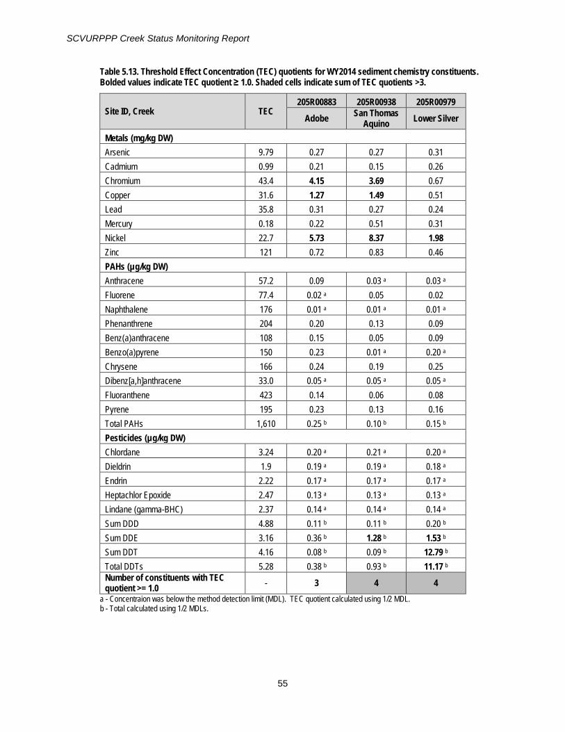
SCVURPPP Creek Status Monitoring Report
Table 5.13. Threshold Effect Concentration (TEC) quotients for WY2014 sediment chemistry constituents. Bolded values indicate TEC quotient ≥ 1.0. Shaded cells indicate sum of TEC quotients >3.
Site ID, Creek TEC 205R00883 205R00938 205R00979
Adobe San Thomas Aquino Lower Silver
Metals (mg/kg DW) Arsenic 9.79 0.27 0.27 0.31 Cadmium 0.99 0.21 0.15 0.26 Chromium 43.4 4.15 3.69 0.67 Copper 31.6 1.27 1.49 0.51 Lead 35.8 0.31 0.27 0.24 Mercury 0.18 0.22 0.51 0.31 Nickel 22.7 5.73 8.37 1.98 Zinc 121 0.72 0.83 0.46 PAHs (µg/kg DW) Anthracene 57.2 0.09 0.03 a 0.03 a Fluorene 77.4 0.02 a 0.05 0.02 Naphthalene 176 0.01 a 0.01 a 0.01 a Phenanthrene 204 0.20 0.13 0.09 Benz(a)anthracene 108 0.15 0.05 0.09 Benzo(a)pyrene 150 0.23 0.01 a 0.20 a Chrysene 166 0.24 0.19 0.25 Dibenz[a,h]anthracene 33.0 0.05 a 0.05 a 0.05 a Fluoranthene 423 0.14 0.06 0.08 Pyrene 195 0.23 0.13 0.16 Total PAHs 1,610 0.25 b 0.10 b 0.15 b Pesticides (µg/kg DW) Chlordane 3.24 0.20 a 0.21 a 0.20 a Dieldrin 1.9 0.19 a 0.19 a 0.18 a Endrin 2.22 0.17 a 0.17 a 0.17 a Heptachlor Epoxide 2.47 0.13 a 0.13 a 0.13 a Lindane (gamma-BHC) 2.37 0.14 a 0.14 a 0.14 a Sum DDD 4.88 0.11 b 0.11 b 0.20 b Sum DDE 3.16 0.36 b 1.28 b 1.53 b Sum DDT 4.16 0.08 b 0.09 b 12.79 b Total DDTs 5.28 0.38 b 0.93 b 11.17 b Number of constituents with TEC quotient >= 1.0 - 3 4 4
a - Concentraion was below the method detection limit (MDL). TEC quotient calculated using 1/2 MDL. b - Total calculated using 1/2 MDLs.
55

SCVURPPP Creek Status Monitoring Report
Table 5.14. Probable Effect Concentration (PEC) quotients for WY2014 sediment chemistry constituents. Bolded values indicate individual PEC quotients > 1.0; mean PEC quotients did not exceed 0.5.
Site ID, Creek PEC 205R00883 205R00938 205R00979
Adobe San Thomas Aquino Lower Silver
Metals (mg/kg DW) Arsenic 33.0 0.08 0.08 0.09 Cadmium 4.98 0.04 0.03 0.05 Chromium 111 1.62 1.44 0.26 Copper 149 0.27 0.32 0.11 Lead 128 0.09 0.08 0.07 Mercury 1.06 0.04 0.09 0.05 Nickel 48.6 2.67 3.91 0.93 Zinc 459 0.19 0.22 0.12 PAHs (µg/kg DW) Anthracene 845 0.01 0.00 a 0.00 a Fluorene 536 0.00 a 0.01 0.00 Naphthalene 561 0.00 a 0.00 a 0.00 a Phenanthrene 1170 0.03 0.02 0.02 Benz(a)anthracene 1050 0.02 0.01 0.01 Benzo(a)pyrene 1450 0.02 0.00 a 0.02 a Chrysene 1290 0.03 0.02 0.03 Fluoranthene 2230 0.03 a 0.01 a 0.01 a Pyrene 1520 0.03 0.02 0.02 Total PAHs 22,800 0.02 b 0.01 b 0.01 b Pesticides (µg/kg DW) Chlordane 17.6 0.04 a 0.04 a 0.04 a Dieldrin 61.8 0.01 a 0.01 a 0.01 a Endrin 207.0 0.00 a 0.00 a 0.00 a Heptachlor Epoxide 16 0.02 a 0.02 a 0.02 a Lindane (gamma-BHC) 4.99 0.07 a 0.07 a 0.07 a Sum DDD 28 0.02 b 0.02 b 0.03 b Sum DDE 31.3 0.04 b 0.13 b 0.15 b Sum DDT 62.9 0.01 b 0.01 b 0.85 b Total DDTs 572 0.00 b 0.01 b 0.10 b Mean PEC Quotient - 0.20 0.24 0.11
a - concentration was below the method detection limit (MDL). PEC quotient calculated using 1/2 MDL. b - Total calculated using 1/2 MDLs.
56

SCVURPPP Creek Status Monitoring Report
Table 5.15. Calculated pyrethroid toxic unit (TU) equivalents for WY2014 pyrethroid concentrations. Bolded cells indicate exceedance of LC50. Shaded cells indicate sum of TUs >1.
Pyrethroid Unit LC50 205R00883 205R00938 205R00979
Adobe San Thomas Aquino Lower Silver
Bifenthrin µg/g dw 0.52 0.33 2.88 3.27 Cyfluthrin µg/g dw 1.08 0.04 a 0.62 0.44 Cypermethrin µg/g dw 0.38 0.12 a 0.13 a 1.26 a Deltamethrin µg/g dw 0.79 0.09 a 0.09 a 0.09 a Esfenvalerate µg/g dw 1.54 0.03 a 0.03 a 0.03 a Lambda-Cyhalothrin µg/g dw 0.45 0.12 a 0.13 a 0.12 a Permethrin µg/g dw 10.83 0.03 b 0.12 b 0.16 b Sum of Toxic Unit Equivalents per Site - - 0.76 4.00 5.36
a - concentration was below the method detection limit (MDL). PEC quotient calculated using 1/2 MDL. b - Total calculated using 1/2 MDLs.
5.4.6 Temperature Summary statistics for water temperature data collected at five sites in Guadalupe Creek and five sites in Stevens Creek during WY2014 are shown in Table 5.16 and Table 5.17, respectively. Station locations are mapped in Figures 5.11 and 5.12. Hourly temperature data was collected between April and September, with the exceptions of sites 205GUA229 and 205STE095, which were retrieved in June and July, respectively, due to dry channel conditions.
Table 5.16. Descriptive statistics for continuous water temperature measured in Guadalupe Creek at five sites during WY2014.
Site 205GUA229 205GUA218 205GUA213 205GUA210 205GUA205 Start Date 4/29/2014 4/29/2014 4/29/2014 4/29/2014 4/29/2014
End Date 6/14/2014 9/29/2014 9/29/2014 9/29/2014 9/29/2014
Temp
eratu
re (
°C)
Minimum 10.1 11.0 10.7 10.0 11.6
Median 13.7 18.9 17.5 17.6 18.2
Mean 13.8 18.2 16.8 17.3 17.8
Maximum 18.4 23.3 20.4 22.9 21.8 Max 7-day
Mean 16.0 21.0 18.7 20.1 20.4
N 1233 3809 3809 3810 3810
57

SCVURPPP Creek Status Monitoring Report
Table 5.17. Descriptive statistics for continuous water temperature measured in Stevens Creek at five sites during WY2014.
Site 205STE105 205STE95 205STE70 205STE65 205STE64 Start Date 4/29/2014 4/29/2014 4/29/2014 4/29/2014 4/29/2014
End Date 9/28/2014 7/13/14 9/29/2014 9/29/2014 9/29/2014
Temp
eratu
re (
°C)
Minimum 9.4 9.5 11.3 11.2 12.5
Median 14.7 15.4 18.7 17.5 18.1
Mean 14.6 15.3 18.0 17.1 18.0
Maximum 19.5 21.2 23.0 21.2 24.3 Max 7-day
Mean 17.0 17.5 21.2 19.9 20.2
N 3790 1940 3810 3810 3810
58
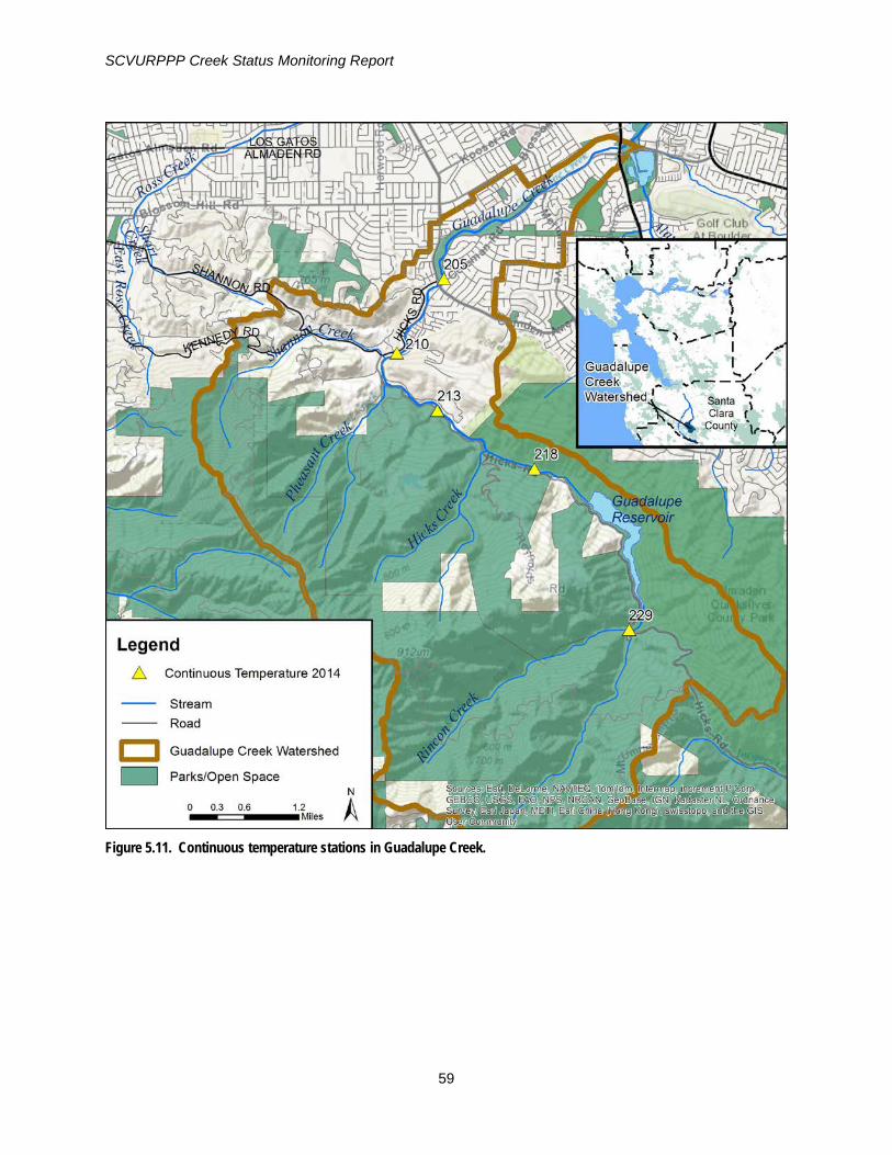
SCVURPPP Creek Status Monitoring Report
Figure 5.11. Continuous temperature stations in Guadalupe Creek.
59

SCVURPPP Creek Status Monitoring Report
Figure 5.12. Continuous temperature stations in Stevens Creek.
60

SCVURPPP Creek Status Monitoring Report
The monitoring results from Guadalupe Creek suggest that the reservoir has some influence on the water temperature measured in the creek (Table 5.16). The lowest median temperature (13.7 °C) was measured at the site approximately 0.5 mile upstream of the Guadalupe Reservoir (205GUA229) and the highest median temperature (18.9 °C) was measured at the site approximately 0.5 mile downstream of the reservoir (205GUA218). However, temperature was only collected at the upper site until June 14th due to dry channel conditions. As a result, the median temperatures at the upper site should only be compared to the lower site for the monitoring period prior to June. For this time period, the median temperatures for sites above reservoir and below reservoir were 13.7 °C and 15.2 °C, respectively. Water temperatures for the sites just upstream and downstream Guadalupe Reservoir are plotted in Figure 5.13. The daily maximum and minimum air temperatures, collected from a local weather station, are also shown on the figure. Stream flow data (not shown) measured below the dam was consistently less than 1 cfs throughout the monitoring period. Water temperature downstream of the dam is likely influenced by increased air temperatures through the dry season, as well as increased water temperatures within the reservoir. Due to extreme drought conditions during WY2014, the water levels in Guadalupe Reservoir were much lower than normal, which likely resulted in elevated temperatures in water released below the dam.
Figure 5.13. Water temperature collected directly upstream and downstream of Guadalupe Creek during WY 2014. Minimum and maximum air temperature data, collected from local weather station, are also shown.
The temperature pattern in Stevens Creek was similar to Guadalupe Creek with the highest median temperatures measured at the site directly downstream of the reservoir (18.7 °C) and the lowest median temperature (14.7 °C) occurring at the upper elevation site (Table 5.17). Note the upper elevation site was approximately three miles upstream of the reservoir. The temperature collected at these two sites occurred over the same period (April through September). Similar to Guadalupe Creek, drying conditions upstream of the Stevens Creek Reservoir occurred by July and water levels in the reservoir became extremely low. Box plots illustrating the distribution of water temperature data for 2014 at five sites in Guadalupe Creek and five sites in Stevens Creek, are shown in Figures 5.14 and 5.15, respectively. The acute temperature threshold (24.0 °C) is shown on both figures. Temperatures were below the acute threshold at all sites in both watersheds, with the exception of a small percentage of the data collected at the Backberry Farm site in Stevens Creek (STE064).
Box plots illustrating the distribution of water temperature data, calculated as the 7-day mean, for five sites in Guadalupe Creek and five sites in Stevens Creek are shown in Figures 5.16 and 5.17, respectively. The chronic (maximum 7-day mean) temperature (MWAT) threshold (19.0 °C) is shown in both figures. Trigger analysis of temperature data using the MWAT threshold is included in Table 5.25. A trigger is defined when the MWAT exceeds the threshold for more than 20% of records at a single site.
Triggers for temperature were exceeded in Guadalupe Creek at the site directly downstream of the reservoir (GUA218) and the lowest elevation site downstream of Coleman Avenue (GUA205) with 49% and 28%, respectively, of the measurements exceeding the MWAT threshold (Table 5.18). A similar
0
5
10
15
20
25
30
35
40
4/20 4/27 5/4 5/11 5/18 5/25 6/1 6/8 6/15 6/22 6/29 7/6 7/13 7/20 7/27 8/3 8/10 8/17 8/24 8/31 9/7 9/14 9/21 9/28 10/5
Tem
pera
ture
(ºC)
205GUA229 205GUA218 Daily Maximum Air Temperature Daily Minimum Air Temperature
61

SCVURPPP Creek Status Monitoring Report
pattern was observed in Stevens Creek, with triggers exceeded at the site below the dam (STE070) and lowest elevation site at Blackberry Farm, with 54% and 30%, respectively, of the measurements exceeding the MWAT threshold.
Figure 5.14. Box plots of water temperature data collected at five stream locations in Guadalupe Creek, Santa Clara County, from April through September 2014.
Figure 5.15. Box plots of water temperature data collected at five stream locations in Stevens, Santa Clara County, from April through September 2014.
205GUA229 205GUA218 205GUA213 205GUA210 205GUA205
Tem
pera
ture
(°C
)
0
5
10
15
20
25
30Instantaneous Maximum for Salmonids (24.0°C)
Upstream ---------------------------------> Downstream
205STE105 205STE095 205STE070 205STE065 205STE064
Tem
pera
ture
(°C
)
0
5
10
15
20
25
30Instantaneous Maximum for Salmonids (24.0 C)
Upstream ---------------------------------> Downstream
62

SCVURPPP Creek Status Monitoring Report
Figure 5.16. Box plots of water temperature data, calculated as the 7-day mean, collected at five stream locations in Guadalupe Creek, Santa Clara County, from April through September 2014.
Figure 5.17. Box plots of water temperature data, calculated as the 7-day mean, collected at five stream locations in Stevens Creek, Santa Clara County, from April through September 2014.
205GUA229 205GUA218 205GUA213 205GUA210 205GUA205
Tem
pera
ture
(°C
)
0
5
10
15
20
25
30MWAT for Steelhead (19.0°C)
Upstream ---------------------------------> Downstream
205STE105 205STE095 205STE070 205STE065 205STE064
Tem
pera
ture
(°C
)
0
5
10
15
20
25
30MWAT for Steelhead (19.0 C)
Upstream ---------------------------------> Downstream
63

SCVURPPP Creek Status Monitoring Report
Table 5.18. Percent of water temperature data measured between April – September, 2014 that exceeded MWAT maximum threshold value (19 °C) at the ten temperature sites monitored in Guadalupe Creek and Stevens in Santa Clara County.
Site ID Creek Site Name Percentage
results MWAT > 19º
Trigger (>20%)
Exceeded?
205GUA229
Guadalupe Creek
Confluence with Rincon Creek 0% No
205GUA218 Downstream of the Horse Stable 49% Yes
205GUA213 At the Fish Ladder 0% No
205GUA210 At Shannon Oaks 17% No
205GUA205 At Camden and Coleman 30% Yes 205STE105
Stevens Creek
Upstream of the reservoir 0% No 205STE95 At Sycamore Group area 0% No 205STE70 At the SCVWD gage 54% Yes 205STE65 At McClellan Ranch 14% No 205STE64 At Blackberry Farm 28% Yes
The reach in Stevens Creek between Blackberry Farm and Stevens Creek Reservoir was identified as having the best quality steelhead spawning and juvenile rearing habitat within the Stevens Creek watershed (Stillwater 2004). The limiting factors analysis study evaluated water temperature data collected by the SCVWD during WY2000 and determined that temperatures downstream of the dam were relatively warm, but within the range to support a steelhead population. Across eight monitoring sites below Stevens Creek dam, the daily average temperatures ranged between 11.7 to 21.7 °C (note: raw temperature data was not available to calculate daily averages for any one site). The study concluded that WY2000 was considered an “average” year climatologically suggesting that the stream temperature data was representative of typical conditions below Stevens Creek Reservoir.
The three lowest elevation monitoring sites in Steven Creek are located within the reach that potentially supports steelhead populations. Two of the three sites in this reach had temperatures that exceeded MWAT (19 °C) for steelhead. Water temperatures measured during this study are expected to be higher than what might occur during a more typical year due to antecedent drought conditions causing very low water levels in the Stevens Creek Reservoir and minimal baseflows during the dry season. Additional temperature monitoring during wetter years would provide a useful comparison to data collected during WY2014.
Similar to Stevens Creek, Guadalupe Creek potentially supports steelhead rearing and spawning habitat downstream of the Guadalupe Creek Reservoir. Existing information was not available to evaluate the distribution or abundance of steelhead in Guadalupe Creek, nor to compare temperatures from previous years to temperatures measured during WY2014.
64

SCVURPPP Creek Status Monitoring Report
5.5 General Water Quality Summary statistics for general water quality measurements collected at the three sites in Stevens Creek during two sampling events in WY2014 are listed in Table 5.19. Sampling Event 1 was conducted in May-June and Event 2 was conducted during August 2014. Plots of the data collected during both events in WY2014 are shown in Figure 5.18 and Figure 5.19. Station locations are mapped in Figure 5.12.
5.5.1 Temperature Box plots showing the distribution of 7-day average water temperature data collected at three sites in Stevens Creek during 2014 are shown in Figure 5.20. The chronic (maximum 7-day mean) temperature (MWAT) threshold (19.0 °C) is shown in the figure. Trigger analysis of temperature data using the MWAT threshold is included in Table 5.20. The MWAT threshold was exceeded at site 205STE071 (100% of the data) and site 205STE065 (40% of the data) during the August event.
Table 5.19. Descriptive statistics for daily and monthly continuous water temperature, dissolved oxygen, conductivity, and pH measured at three sites in Stevens Creek during two sampling events in 2014.
Parameter Data Type 205STE105 205STE071 205STE065
June August June August June August
Temp (° C)
Min 10.31 13.5 13.5 20.2 13.1 16.8 Median 13.9 16.5 15.9 22.1 15.8 18.8 Mean 13.8 16.4 16.0 22.2 15.9 18.8 Max 18.4 19.6 19.2 24.6 19.4 20.3 Max 7-day Mean 14.6 17.1 16.5 22.5 16.8 19.3
Dissolved Oxygen (mg/l)
Min 7.6 6.3 4.4 5.5 5.0 4.8 Median 9.0 7.9 6.1 6.4 7.2 7.3 Mean 9.0 7.9 6.0 6.4 7.2 7.3 Max 9.8 9.3 6.7 7.1 9.9 8.7 7-day Avg. Min 8.1 6.8 5.1 5.7 5.8 5.7
pH
Min 7.9 7.9 7.6 7.9 8.1 7.9 Median 8.0 8.0 7.6 7.9 8.3 8.2 Mean 8.0 8.0 7.6 7.9 8.3 8.2 Max 8.1 8.2 7.7 8.0 8.4 8.3
Specific Conductance (uS/cm)
Min 602 619 770 736 751 746 Median 608 627 777 759 761 753 Mean 608 626 777 756 760 752 Max 616 631 782 767 764 752
Total number data points (n) 1235 1424 1240 1425 1443 1427
65

SCVURPPP Creek Status Monitoring Report
Figure 5.18. Continuous water quality data (temperature, dissolved oxygen, pH and specific conductance) collected using sondes at three sites in Stevens Creek during sampling Event 1 in 2014.
66

SCVURPPP Creek Status Monitoring Report
Figure 5.19. Continuous water quality data (temperature, dissolved oxygen, pH and specific conductance) collected using sondes at three sites in Stevens Creek during sampling Event 2 in 2014.
67

SCVURPPP Creek Status Monitoring Report
Figure 5.20. Box plots of 7-day average water temperature data at three stream locations in Stevens Creek, Santa Clara County, during two sampling events in 2014
Table 5.20. Percent of water temperature data measured at three sites in Stevens Creek, Santa Clara County for both events that exceed trigger values identified in Table 4.4.
Site ID Creek Name Site Monitoring
Event Percent results MWAT > 19 °C
Trigger (>20%) Exceeded?
205STE105
Stevens Creek
Above Reservoir June 0% No
August 0% No
205STE071 Below Dam June 0% No
August 100% Yes
205STE065 McClellan Ranch June 0% No
August 40% Yes
Upstream ------------------------> Downstream
205STE105 205STE071 205STE065
Temp
eratu
re (º
C)
0
5
10
15
20
25
30
JuneAugustMWAT for Steelhead (19.0ºC)
68

SCVURPPP Creek Status Monitoring Report
5.5.2 Dissolved Oxygen Box plots showing the distribution of dissolved oxygen data measured at three sites in Stevens Creek during WY2014 are shown in Figure 5.21. The dissolved oxygen WQOs for WARM and COLD Freshwater Habitat are included in the figure. A trigger analysis of dissolved oxygen data using both WQOs is included in Table 5.21. The WQO for COLD (7.0 mg/L) was not met in 98% to 100% of the measurements taken at the site below the dam (STE071) and in 32% to 40% of the measurements taken at McClellan Ranch (STE065) during the WY2014 sampling events (Table 5.28). The WQO for WARM (5.0 mg/L) was infrequently exceeded at the two sites below the dam; however the number of measurements was well below the 20% criteria for trigger.
Figure 5.21. Box plots of dissolved oxygen data collected at three stream locations in Stevens Creek, Santa Clara County, during two sampling events in 2014.
Table 5.21. Percent of dissolved oxygen data measured at three sites in Stevens Creek for both events that exceed triggers.
Upstream ------------------------> Downstream
205STE105 205STE071 205STE065
Diss
olved
Oxy
gen (
mg/L)
0
2
4
6
8
10
12
JuneAugustCold Freshwater WQO (7 mg/L)Warm Freshwater WQO (5 mg/L)
Site ID Creek Name Site Monitoring
Event Percent Results
DO < 5.0 mg/L
Percent Results
DO < 7.0 mg/L
Trigger (>20%)
Exceeded?
205STE105
Stevens Creek
Above Reservoir
June 0% 0% No
August 0% 3% No
205STE071 Below Dam June 0.5 100% Yes (Cold)
August 0% 98% Yes (Cold)
205STE065 McClellan Ranch
June 0.1% 40% Yes (Cold) August 0.3% 32% Yes (Cold)
69
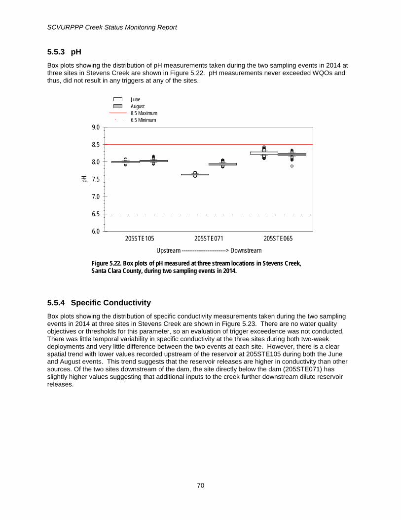
SCVURPPP Creek Status Monitoring Report
5.5.3 pH Box plots showing the distribution of pH measurements taken during the two sampling events in 2014 at three sites in Stevens Creek are shown in Figure 5.22. pH measurements never exceeded WQOs and thus, did not result in any triggers at any of the sites.
Figure 5.22. Box plots of pH measured at three stream locations in Stevens Creek, Santa Clara County, during two sampling events in 2014.
5.5.4 Specific Conductivity Box plots showing the distribution of specific conductivity measurements taken during the two sampling events in 2014 at three sites in Stevens Creek are shown in Figure 5.23. There are no water quality objectives or thresholds for this parameter, so an evaluation of trigger exceedence was not conducted. There was little temporal variability in specific conductivity at the three sites during both two-week deployments and very little difference between the two events at each site. However, there is a clear spatial trend with lower values recorded upstream of the reservoir at 205STE105 during both the June and August events. This trend suggests that the reservoir releases are higher in conductivity than other sources. Of the two sites downstream of the dam, the site directly below the dam (205STE071) has slightly higher values suggesting that additional inputs to the creek further downstream dilute reservoir releases.
Upstream ------------------------> Downstream
205STE105 205STE071 205STE065
pH
6.0
6.5
7.0
7.5
8.0
8.5
9.0
JuneAugust8.5 Maximum6.5 Minimum
70

SCVURPPP Creek Status Monitoring Report
Figure 5.23. Box plots of specific conductivity measured at three stream locations in Stevens Creek, Santa Clara County, during two sampling events in 2014.
5.6 Pathogen Indicators Pathogen indicator densities measured in water samples in WY2014 are listed in Table 5.22.
Table 5.22. Fecal coliform and E. coli levels measured in Santa Clara County during WY2014.
Site ID Creek Name Site Name Fecal Coliform (MPN/100ml)
E. Coli (MPN/100ml) Sample
Date Trigger Threshold (REC-1/REC-2) 400/4,000 410
205GUA050 Los Gatos Creek Lonus Street 500 500 7/8/14 205GUA225 Arroyo Calero Singer Park 300 300 7/8/14 205SAR005 Saratoga Creek Bowers Park 500 500 7/8/14 205STE065 Stevens Creek McClellan Ranch 230 230 7/8/14
205STE071 Stevens Creek Lower Stevens Creek County Park 50 50 7/8/14
All five creeks monitored for pathogen indicators are designated for both contact (REC-1) and non-contact (REC-2) recreation. Although none of the stations could be considered “bathing beaches,” monitoring locations at each creek were selected at city parks or trails that were considered to exhibit high potential for public access. The trigger threshold for fecal coliform and for E. coli concentrations were exceeded at the sites in Los Gatos Creek (205GUA050) and Saratoga Creek (205SAR005). Additional investigations relative to characterizing exposure would be needed to better understand the waterborne pathogen-related risk at these sites.
Upstream ------------------------> Downstream
205STE105 205STE071 205STE065
Spec
ific C
ondu
ctivit
y (µS
/cm)
550
600
650
700
750
800
850
900
JuneAugust
71

SCVURPPP Creek Status Monitoring Report
6.0 CONCLUSIONS The following conclusions from the MRP Creek Status Monitoring conducted during WY2014 in Santa Clara County are based on the management questions presented in Section 1.0:
1) Are water quality objectives, both numeric and narrative, being met in local receiving waters, including creeks, rivers, and tributaries?
2) Are conditions in local receiving water supportive of or likely supportive of beneficial uses?
The first management question is addressed primarily through the evaluation of probabilistic and targeted monitoring data with respect to the triggers defined in Table 4.4. A summary of trigger exceedances observed for each site is presented in Table 6.1. Sites where triggers are exceeded may indicate potential impacts to aquatic life or other beneficial uses and are considered for future evaluation of stressor source identification projects.
The second management question is addressed primarily through calculation of indices of biological integrity (IBI) using benthic macroinvertebrate and algae data collected at probabilistic sites. Biological condition scores were compared to physical habitat and water quality data collected synoptically with bioassessments to evaluate whether any correlations exist that may explain the variation in IBI scores.
Biological Condition
• The California Stream Condition Index (CSCI) tool was used to assess the biological condition for benthic macroinvertebrate data collected at probabilistic sites. Of the 20 sites monitored in WY2014, five sites rated as likely intact condition (CSCI score > 0.92); three sites rated as possibly intact condition (CSCI score 0.79 – 0.92); one site rated as likely altered condition (CSCI score 0.63 – 0.78) and eleven sites rated as very likely altered condition (< 0.63).
• An Algae IBI, based on combination of soft algae and diatom metrics (referred to as “H20”), was used to evaluate benthic algae data collected synoptically with BMIs at probabilistic sites. No condition categories have been developed for “H20” Algae IBI scores. The Algae IBI results should be considered preliminary until additional research shows that these tools perform well for data collected in Santa Clara County.
• Algae IBI scores were not well correlated with CSCI scores (R2 = 0.31), indicating responses of algae to stressors differ compared to BMIs.
• There was very little difference in CSCI scores between perennial (n=16) and non-perennial (n=4) sites. In contrast, Algae IBI scores were generally lower at perennial sites compared to non-perennial sites. Both CSCI scores and Algae IBI scores had good response to different levels of urbanization (calculated as percent impervious area).
• Environmental variables that had significant correlation to CSCI scores include epifaunal substrate score, percent impervious and chloride. Environmental variables that had significant correlation to Algae IBI scores included epifaunal substrate, CRAM score, Unionized Ammonia and Total Kjeldahl Nitrogen).
Nutrients and Conventional Analytes
• Nutrients (nitrogen and phosphorus), algal biomass indicators, and other conventional analytes were measured in samples collected concurrently with bioassessments which are conducted in the spring season. Trigger thresholds for chloride, unionized ammonia, and nitrate were not exceeded.
• Free chlorine and/or total chlorine residual triggers were exceeded at four highly urban probabilistic sites. These results are common under urban land use conditions.
72

SCVURPPP Creek Status Monitoring Report
Water Toxicity
• Water toxicity samples were collected from three sites during two sample events (winter storm event and summer). Although two samples from both sampling events were toxic relative to the Lab Control treatment, no water toxicity samples exceeded MRP trigger thresholds.
Sediment Toxicity
• Sediment toxicity and chemistry samples were collected concurrently with the summer water toxicity samples. None of the sites exceeded the MRP trigger for sediment toxicity. All three sites exceeded the trigger threshold for sediment chemistry as a result of pyrethroid pesticide concentrations. Two sites also exceeded the highly conservative TEC trigger.
Spatial and Temporal Variability of Water Quality Conditions
• Median water temperatures continuously measured in Guadalupe Creek (n=5) and Stevens Creek (n=5) were generally highest at sites downstream of the reservoirs and lowest at sites upstream of the reservoirs. Dry channel conditions occurred upstream of the reservoirs in Guadalupe Creek and Stevens Creek beginning in the months of June and July, respectively.
• Continuous general water quality monitoring was conducted at three sites in Stevens Creek during two two-week periods (June and August. Median dissolved oxygen concentrations were lowest (range 6.0 – 6.4 mg/L) for both sampling events at site 205STE071, located just downstream Stevens Creek Reservoir. Median dissolved oxygen concentrations were relatively consistent at all three sites between spring and late summer sample events.
Potential Impacts to Aquatic Life
• There were no exceedances of the Maximum Weekly Average Temperature (MWAT) threshold at any of the sites upstream of either Guadalupe Creek (n=1) or Stevens Creek (n=2) Reservoirs, suggesting that water temperatures support rearing habitat for resident rainbow trout in these reaches. However, the intermittent flow and dry channel conditions above both reservoirs during the summer and fall season of 2014 would significantly limit the amount of potential habitat available to trout.
• Three of the four sites below Guadalupe Creek Reservoir exceeded the MWAT threshold trigger between 17% and 49% of the time during WY2014. The monitoring location below the fish ladder (site 205GUA105) never exceeded the threshold, suggesting areas downstream of the dam provide habitat with temperatures that are more suitable for steelhead. The three sites below Stevens Creek Reservoir exceeded the MWAT threshold trigger between 14% and 54% of the time during WY2014.
• Cool water releases below dams provide adequate summer rearing conditions in relatively low elevation habitats that historically were too warm to support steelhead or were seasonally dry. The extended drought type conditions during WY2014 have resulted in dramatically low water levels in both Guadalupe and Stevens Creek Reservoirs, resulting in lower than normal baseflows and releases and higher than normal water temperatures downstream of the dam.
• The WQO for DO in waters designated as having cold freshwater habitat (COLD) beneficial uses (i.e., 7.0 mg/L) was not met in 98% - 100% of measurements taken at the site below the dam (205STE071) and was not met in 32% - 40% of measurements taken at McClellan Ranch (205STE065) during both sampling events in 2014. The WQO for WARM (5.0 mg/L) was periodically exceeded, but the total number of exceedences were not above the 20% criteria to cause a trigger.
• Values for pH measured at three Stevens Creek sites during WY2014 were within WQOs.
73

SCVURPPP Creek Status Monitoring Report
Potential Impacts to Water Contact Recreation
• Pathogen indicator densities were measured at five of the probabilistic sites during WY2014. Threshold triggers for fecal coliform and E. coli were exceeded at one site in Los Gatos Creek (205GUA050) and one site in Saratoga Creek (205SAR005).
It is important to recognize that pathogen indicator thresholds are based on human recreation at beaches receiving bacteriological contamination from human wastewater, and may not be applicable to conditions found in urban creeks. As a result, the comparison of pathogen indicator results to water quality objectives and criteria for full body contact recreation, may not be appropriate and should be interpreted cautiously.
Table 6.1. Summary of SCVURPPP Trigger Threshold Exceedance Analysis, WY2014. “No” indicates samples were collected but did not exceed the MRP trigger; “Yes” indicates an exceedance of the MRP trigger.
Station Number Creek
Bioa
sses
smen
t
Nutri
ents
”
Chlo
rine
Wat
er T
oxici
ty
Sedi
men
t To
xicity
Sedi
men
t Ch
emist
ry
Tem
pera
ture
Cont
inuo
us W
Q
Path
ogen
In
dica
tors
205R00266 Limekiln Creek Yes No No -- -- -- -- -- -- 205R00330 Hick's Creek No No No -- -- -- -- -- -- 205R00362 Lyndon Canyon No No No -- -- -- -- -- -- 205R00394 Austrian Gulch No No No -- -- -- -- -- -- 205R00851 Los Coches Creek Yes No No -- -- -- -- -- -- 205R00883 Adobe Creek No No No No No Yes -- -- -- 205R00915 Thompson Creek Yes No No -- -- -- -- -- -- 205R00938 San Tomas Aquino Creek No No No No No Yes -- -- -- 205R00979 Lower Silver Creek Yes No Yes No No Yes -- -- -- 205R01027 Guadalupe River Yes No No -- -- -- -- -- -- 205R01091 Saratoga Creek Yes No Yes -- -- -- -- -- Yes 205R01098 Guadalupe Creek No No No -- -- -- -- -- -- 205R01187 Stevens Creek Yes No Yes -- -- -- -- -- No 205R01226 Los Gatos Creek Yes No No -- -- -- -- -- -- 205R01299 Arroyo Aguague No No No -- -- -- -- -- -- 205R01306 Ross Creek Yes No Yes -- -- -- -- -- -- 205R01434 Arroyo Calero No No No -- -- -- -- -- No 205R01443 Stevens Creek Yes No No -- -- -- -- -- No 205R01539 Los Gatos Creek Yes No No -- -- -- -- -- Yes 205R01578 San Tomas Aquino Creek Yes No No -- -- -- -- -- -- 205STE064 Stevens Creek -- -- -- -- -- -- Yes -- -- 205STE065 Stevens Creek -- -- -- -- -- -- No Yes -- 205STE071 Stevens Creek -- -- -- -- -- -- Yes Yes -- 205STE095 Stevens Creek -- -- -- -- -- -- No -- -- 205STE105 Stevens Creek -- -- -- -- -- -- No No -- 205GUA205 Guadalupe Creek -- -- -- -- -- -- Yes -- -- 205GUA210 Guadalupe Creek -- -- -- -- -- -- No -- -- 205GUA213 Guadalupe Creek -- -- -- -- -- -- No -- -- 205GUA218 Guadalupe Creek -- -- -- -- -- -- Yes -- -- 205GUA229 Guadalupe Creek -- -- -- -- -- -- No -- --
74

SCVURPPP Creek Status Monitoring Report
Management Implications The Program’s Creek Status Monitoring program (consistent with MRP Provision C.8.c) focuses on assessing the water quality condition of urban creeks in the Santa Clara Valley and identifying stressors and sources of impacts observed. Although the sample size from WY2014 (overall n=20; urban n=16) is not sufficient to develop statistically representative conclusions regarding the overall condition of all creeks, it is clear that most urban portions have likely or very likely altered populations of aquatic life indicators (e.g., aquatic macroinvertebrates). These conditions are likely the result of long-term changes in stream hydrology, channel geomorphology and in-stream habitat complexity, and other modifications to the watershed and riparian areas associated with urban development that has occurred over the past 50 plus years in the contributing watersheds. Additionally, water quality conditions associated with pyrethroid pesticides present in creek sediments at concentrations known to adversely affect sensitive aquatic organisms (i.e., LC50s), and episodic or site specific increases temperature and decreased dissolved oxygen (particularly in lower creek reaches) are not optimal for aquatic life in local creeks.
The Program and its Co-permittees are actively implementing many stormwater management programs to address these and other stressors and associated sources of water quality conditions observed in local creeks, with the goal of protecting these natural resources. For example:
• In compliance with MRP provision C.3, new and redevelopment projects in the Bay Area are now designed to more effectively reduce water quality and hydromodification impacts associated with urban development. Low impact develop (LID) methods, such as rainwater harvesting and use, infiltration and biotreatment are now required as part of development and redevelopment projects. These LID measures are expected to reduce the impacts of urban runoff and associated impervious surfaces on stream health.
• In compliance with MRP provision C.9, the Program and Co-permittees are implementing pesticide toxicity control programs that focus on source control and pollution prevention measures. The control measures include the implementation of integrated pest management (IPM) policies/ordinances, public education and outreach programs, pesticide disposal programs, the adoption of formal State pesticide registration procedures, and sustainable landscaping requirements for new and redevelopment projects. Through these efforts, it is estimated that the amount of pyrethroids observed in urban stormwater runoff will decrease by 80-90% over time, and in turn significantly reduce the magnitude and extent of toxicity in local creeks.
• Trash loadings to local creeks are also being reduced through implementation of new control measures in compliance with MRP provision C.10 and other efforts by Co-permittees to reduce the impacts of illegal dumping directly into waterways. These actions include the installation and maintenance of trash capture systems, the adoption of ordinances to reduce the impacts of litter prone items, enhanced institutional controls such as street sweeping, and the on-going removal and control of direct dumping.
• In compliance with MRP provisions C.2 (Municipal Operations), C.4 (Industrial and Commercial Site Controls), C.5 (Illicit Discharge Detection and Elimination), and C.6 (Construction Site Controls) Co-permittees continue to implement programs that are designed to prevent non-stormwater discharges during dry weather and reduce the exposure of contaminants to stormwater and sediment in runoff during rainfall events.
• Additionally, in compliance with MRP provision C.13, copper in stormwater runoff is reduced through implementation of controls such as architectural and site design requirements, street sweeping, and participation in statewide efforts to significantly reduce the level of copper vehicle brake pads.
In addition to the Program and Co-permittee controls implemented in compliance with the MRP, numerous other efforts and programs designed to improve the biological, physical and chemical condition of local creeks are underway (e.g., SCVWD’s 2010 Flood Protection and Stream Stewardship Master Plan). Through the continued implementation of MRP-associated and other watershed stewardship
75

SCVURPPP Creek Status Monitoring Report
programs, SCVURPPP anticipates that stream conditions and water quality in local creeks will continue to improve overtime. In the near term, toxicity observed in creeks should decrease as pesticide regulations better incorporate water quality concerns during the pesticide registration process. In the longer term, control measures implemented to “green” the “grey” infrastructure and disconnect impervious areas constructed over the course of the past 50 plus years will take time to implement. Consequently, it may take several decades to observe the outcomes of these important, large-scale improvements to our watersheds in our local creeks. Long-term creek status monitoring programs designed to detect these changes over time are therefore beneficial to our collective understanding of the condition and health of our local waterways.
76

SCVURPPP Creek Status Monitoring Report
7.0 REFERENCES Atkinson, K. 2011. Evaluating Water Temperature and Turbidity Effects on Steelhead Life History
Tactics in Alameda Creek Watershed. Technical Memorandum. Alameda Creek Fisheries Restoration Workgroup.
Bay Area Stormwater Management Agency Association (BASMAA) Regional Monitoring Coalition. 2012. RMC Creek Status and Long-Term Trends Monitoring Plan.
Bay Area Stormwater Management Agency Association (BASMAA) Regional Monitoring Coalition. 2014a. Creek Status Monitoring Program Quality Assurance Project Plan, Final Draft Version 2. Prepared for BASMAA by EOA, Inc. on behalf of the Santa Clara Urban Runoff Pollution Prevention Program and the San Mateo Countywide Water Pollution Prevention Program, Applied Marine Sciences on behalf of the Alameda Countywide Clean Water Program, and Armand Ruby Consulting on behalf of the Contra Costa Clean Water Program. 80 pp plus appendices.
Bay Area Stormwater Management Agency Association (BASMAA) Regional Monitoring Coalition. 2014b. Creek Status Monitoring Program Standard Operating Procedures Version 2. Prepared for BASMAA by EOA, Inc. on behalf of the Santa Clara Urban Runoff Pollution Prevention Program and the San Mateo Countywide Water Pollution Prevention Program, Applied Marine Sciences on behalf of the Alameda Countywide Clean Water Program, and Armand Ruby Consulting on behalf of the Contra Costa Clean Water Program. 203 pp.
Bay Area Stormwater Management Agency Association (BASMAA) Regional Monitoring Coalition. 2013. Urban Creeks Monitoring Report Water Years 2012. Submitted pursuant to Provision C.8.g.iii of Order R2-2009-0074 on behalf of all Permittees.
Barbour, M.T., J. Gerritsen, B.D. Snyder, and J.B. Stribling. 1999. Rapid Bioassessment Protocols for Use in Streams and Wadeable Rivers: Periphyton, Benthic Macroinvertebrates and Fish, Second Edition. EPA 841-B-99-002. U.S. Environmental Protection Agency; Office of Water; Washington, D.C.
Beller E.E., Grossinger R.M., Nicholson M., and Salomon M.N. 2012. Upper Penitencia Creek Historical Ecology Assessment. A report of SFEI’s Historical Ecology Program, SFEI Publication #664, San Francisco Estuary Institute, Richmond, CA.
Buchan, L. A. J., R. A. Leidy, and M. K. Hayden. 1999. Aquatic resource characterization of Western Mt. Hamilton Stream fisheries. Prepared by Eisenberg, Olivieri & Associates in association with United States Environmental Protection Agency, for The Nature Conservancy, Sunnyvale, California.
Center for Watershed Protection. 2005. Urban Subwatershed Restoration Manual Series, No. 10 Unified Stream Assessment: A User’s Manual. Version 2.0. Center for Watershed Protection. Ellicot City, Maryland. February 2005.
Collins, J.N., E.D. Stein, M. Sutula, R. Clark, A.E. Fetscher, L. Grenier, C. Grosso, and A. Wiskind. 2008. California Rapid Assessment Method (CRAM) for Wetlands, v. 5.0.2. 157 pp.
Fetscher, A.E, L. Busse, and P.R. Ode. 2009. Standard Operating Procedures for Collecting Stream Algae Samples and Associated Physical Habitat and Chemical Data for Ambient Bioassessments in California. California State Water Resources Control Board Surface Water Ambient Monitoring Program (SWAMP) Bioassessment SOP 002. (Updated May 2010)
Fetscher, A.E., R. Stancheva, J.P. Kociolek, R.G. Sheath, E. Stein, R.D. Mazo and P. Ode. 2013a. Development and comparison of stream indices of biotic integrity using diatoms vs. non-diatom algae vs. a combination. Journal of Applied Phycology. Volume 25 no. 4. August 2013.
77

SCVURPPP Creek Status Monitoring Report
Fetscher, A.E., M.A. Sutula, L.B. Busse and E.D. Stein. 2013b. Condition of California Perennial, Wadeable Streams Based on Algal Indicators. Final Technical Report 2007-11. Prepared by Southern California Coastal Water Research Project and San Diego Regional Water Quality Control Board. Prepared for California State Water Board.
Grossinger, RM, Askevold R, Striplen CJ, Brewster E, Pearce S, Larned K, McKee LJ, Collins JN. 2006. Coyote Creek Watershed Historical Ecology Study: Historical Conditions and Landscape Change in the Eastern Santa Clara Valley, California. San Francisco Estuary Institute. Contribution No. 426. January 2006.
Herbst, D.B., and E.L. Silldorff. 2009. Development of a benthic macroinvertebrate index of biological integrity (IBI) for stream assessments in the Eastern Sierra Nevada of California. Sierra Nevada Aquatic Research Lab. Mammoth Lakes, CA Hill et al. 2000
Karr and Chu 1999. Restoring Life in Running Waters: Better Biological Monitoring. Island Press, Covelo, California.
Leidy, R.A., G.S. Becker, B.N. Harvey. 2005. Historical distribution and current status of steelhead/rainbow trout (Oncorhynchus mykiss) in streams of the San Francisco Estuary, California. Center for Ecosystem Management and Restoration, Oakland, CA.
MacDonald, D.D., C.G. Ingersoll, T.A. Berger. 2000. Development and Evaluation of Consensus-Based Sediment Quality Guidelines for Freshwater Ecosystems. Arch. Environ. Contam. Toxicol. 39, 20-31.
Mattern, D. and .J.M. Sowers. 2003. Baseline Development for Hydrograph Modification Program. Prepared by Mattern & Assoc. and William Lettis & Associates. Prepared for the Santa Clara Valley Water District. December 23, 2003.
Mazor, R.D., A. Rehn, P.R. Ode, M. Engeln, K. Schiff, E. Stein, D. Gillett, D. Herbst, C.P. Hawkins. In review.. Bioassessment in complex environments: Designing an index for consistent meaning in different settings
Moyle, P. B. 2000. Inland Fishes of California. 2nd. edition. University of California Press, Berkeley, California.
Moyle, P.B., J.A. Israel, and S.E. Purdy. 2008. Salmon, Steelhead and Trout in California: Status of an Emblematic Fauna. A report commissioned by Cal Trout 2008.
Myrick, C. A. and J.J. Cech, Jr. 2001. Bay-Delta Modeling Forum. Technical publication 01-1. Temperature effects on Chinook salmon and steelhead: a review focusing on California’s Central Valley populations. Available at: http://www.pacificorp.com/File/File43061.pdf.
Ode, P.R., A. Rehn, and J. May. 2005. Quantitative Tool for Assessing the Integrity of Southern Coastal California Streams, Environmental Management Vol. 35, No. 4, pp. 493-504.
Ode, P.R. 2007. Standard Operating Procedures for Collection Macroinvertebrate Samples and Associated Physical and Chemical Data for Ambient Bioassessments in California. California State Water Resources Control Board Surface Water Ambient Monitoring Program (SWAMP) Bioassessment SOP 001.
Ode, P.R., T.M. Kincaid, T. Fleming and A.C. Rehn. 2011. Ecological Condition Assessments of California’s Perennial Wadeable Streams: Highlights from the Surface Water Ambient Monitoring Program’s Perennial Streams Assessment (PSA) (2000-2007). A Collaboration between the State Water Resources Control Board’s Non-Point Source Pollution Control Program (NPS Program), Surface Water Ambient Monitoring Program (SWAMP), California Department of Fish and Game Aquatic Bioassessment Laboratory, and the U.S. Environmental Protection Agency.
Rehn, A.C., P.R. Ode, and J.T. May. 2005. Development of a benthic index of biotic integrity (B-IBI) for wadeable streams in northern coastal California and its application to regional 305(b) assessment. Report to the State Water Resources Control Board. California Department of Fish. Rancho Cordova, CA.
78

SCVURPPP Creek Status Monitoring Report
Rehn, A.C., J.T. May and P.R. Ode. 2008. An Index of Biotic Integrity (IBI) for Perennial Streams in California’s Central Valley. Report to the State Water Resources Control Board. California Department of Fish. Rancho Cordova, CA.
Railsback, S.F. and K.A. Rose. 1999. Bioenergetics modeling of stream trout growth: temperature and food consumption effects. Trans. Am. Fish. Soc. 128:241-256.
San Francisco Regional Water Quality Control Board (SFRWQCB). 2009. Municipal Regional Stormwater NPDES Permit. Order R2-2009-0074, NPDES Permit No. CAS612008. 125 pp plus appendices.
San Francisco Regional Water Quality Control Board (SFRWQCB). 2012. The Reference Site Study and the Urban Gradient Study Conducted in Selected San Francisco Bay Region Watersheds in 2008-2010 (Years 8 to 10). Surface Water Ambient Monitoring Program, San Francisco Bay Regional Water Quality Control Board, Oakland, CA.
San Francisco Regional Water Quality Control Board (SFRWQCB). 2013. Water Quality Control Plan. (Basin Plan). http://www.waterboards.ca.gov/sanfranciscobay/basin_planning.shtml.
San Mateo Countywide Water Pollution Prevention Program. 2000. Characterization of Imperviousness and Creek Channel Modifications for Six Watersheds in San Mateo County. Prepared by EOA, Inc. August 30, 2000.
Santa Clara Valley Urban Runoff Pollution Prevention Program (SCVURPPP). 2003. Watershed monitoring and assessment summary report, submitted in fulfillment of NPDES permit provision C.10 (b), Sunnyvale, California.
Santa Clara Valley Urban Runoff Pollution Prevention Program (SCVURPPP). 2007. Watershed Assessment and Sediment Impact Analysis; Saratoga Creek, Santa Clara County. Prepared by EOA, Inc. for SCVURPPP. Draft Report July 17, 2007.
Santa Clara Valley Urban Runoff Pollution Prevention Program (SCVURPPP). 2013. Local Urban Creeks Status Monitoring Report, Water Year 2012 (October 2011 – September 2012. March 15, 2013.
Santa Clara Valley Urban Runoff Pollution Prevention Program (SCVURPPP). 2014. Part A of the Integrated Monitoring Report.
Santa Clara Valley Water District. 2006. Coyote Creek: Montague Ex. To Interstate 280 Baseline Fisheries Habitat Study. Prepared by Entrix, Inc. November 16, 2006.
Santa Clara Valley Water District. 2008. Mid-Coyote Flood Protection Project Baseline Fisheries Report Year 2 2008.
Santa Clara Valley Water District. 2011. Stream Ecosystem Condition Profile: Coyote Creek Watershed. San Jose, CA. 103 pp plus appendices.
Smith, J.J. and H.W. Li. 1983. Energetic factors influencing foraging tactics of juvenile steelhead trout, Salmo gairdneri. Pp. 173-180 in D.L.G. Noakes et al. (eds.), Predators and Prey in Fishes. Dr. W. Junk Publishers, The Hague.
Smith, J. 2001. Potential Fisheries in Selected Santa Clara County Streams. Data provided to the Santa Clara Valley Water District.
Solek, C.W., E.D. Stein, and M. Sutula. 2011. Demonstration of an integrated watershed assessment using a three-tiered assessment framework. Wetlands Ecol Manage (2011)19:459-474.
Stevens, D.L.Jr., and A.R. Olsen. 2004. Spatially Balanced Sampling of Natural Resources. Journal of the American Statistical Association 99(465):262-278.
Stillwater Sciences. 2006. Upper Penitencia Creek Limiting Factors Analysis, Final Report. Prepared for Santa Clara Valley Urban Runoff Pollution Prevention Program (Program Managers, EOA, Inc.). 72 pp plus figures and appendices.
79

SCVURPPP Creek Status Monitoring Report
Sullivan, K., Martin, D.J., Cardwell, R.D., Toll, J.E., and S. Duke. 2000. An analysis of the effects of temperature on salmonids of the Pacific Northwest with implications for selecting temperature criteria. Sustainable Ecosystems Institute, Portland, OR. December 2000.
Sogard, Susan M., Merz, Joseph E., Satterthwaite, William H., Beakes, Michael P., Swank, David R., Collins, Erin M., Titus, Robert G. and Mangel, Marc (2012): Contrasts in Habitat Characteristics and Life History Patterns of Oncorhynchus mykiss in California's Central Coast and Central Valley, Transactions of the American Fisheries Society, 141:3, 747-760.
USEPA. 1977. Temperature criteria for freshwater fish: protocol and procedures. Ecological Research Series., U.S. Environmental Protection Agency, EPA-600/3-77-061. 130 pp. [Also cited as Brungs and Jones. 1977]
USEPA. 2000. U.S. Environmental Protection Agency Water Quality Standards; Establishment of Numeric Criteria for Priority Toxic Pollutants for the State of California. 40 CFR Part 131. Federal Register: May 18, 2000 (Volume 65, Number 97), Pages 31681-31719
USEPA. 2009. U.S. Environmental Protection Agency Office of Water, National Recommended Water Quality Criteria <http://water.epa.gov/scitech/swguidance/standards/current/index.cfm>http://water.epa.gov/scitech/swguidance/standards/current/index.cfm
USEPA. 2012. Recreational Water Quality Criteria. Office of Water 820-F-12-058.
80
SCVURPPP Creek Status Monitoring Report
ATTACHMENTS
81

SCVURPPP Creek Status Monitoring Report
Attachment A Site Evaluation Details
82

SCVURPPP Creek Status Monitoring Report
Attachment A. Summary of site evaluation results between WY 2012 -2014.
Station Code Stratum Agency
Code Year
Evaluated Target Status Code
Target Status Detail
204R00013 SC_R2_Nonurb SCVURPPP 2012 TNS TNS_PD 204R00018 SC_R2_Nonurb SCVURPPP 2012 TNS TNS_PD 204R00029 SC_R2_Nonurb SCVURPPP 2012 TNS TNS_PD 204R00045 SC_R2_Nonurb SCVURPPP 2012 TNS TNS_PD 204R00061 SC_R2_Nonurb SCVURPPP 2012 TNS TNS_PD 204R00077 SC_R2_Nonurb SCVURPPP 2012 NT NT_NLSF 204R00082 SC_R2_Nonurb SCVURPPP 2013 TNS TNS_DIST
204R00083 SC_R2_Nonurb SWAMP 2013 NT NT_NLSF 204R00093 SC_R2_Nonurb SCVURPPP 2013 NT NT_NLSF 204R00109 SC_R2_Nonurb SWAMP 2013 TNS TNS_DIST 204R00121 SC_R2_Nonurb SCVURPPP 2013 NT NT_NLSF 204R00125 SC_R2_Nonurb SCVURPPP 2013 TNS TNS_PD 204R00130 SC_R2_Nonurb SCVURPPP 2013 TNS TNS_PD 204R00141 SC_R2_Nonurb SCVURPPP 2013 NT NT_NLSF 204R00149 SC_R2_Nonurb SCVURPPP 2013 NT NT_NLSF 204R00157 SC_R2_Nonurb SCVURPPP 2013 NT NT_NLSF 204R00173 SC_R2_Nonurb SCVURPPP 2013 TNS TNS_PD 204R00185 SC_R2_Nonurb SCVURPPP 2013 NT NT_NLSF 204R00189 SC_R2_Nonurb SCVURPPP 2013 T Target 204R00194 SC_R2_Nonurb SCVURPPP 2013 TNS TNS_DIST
204R00198 SC_R2_Nonurb SCVURPPP 2013 NT NT_NLSF 204R00205 SC_R2_Nonurb SCVURPPP 2013 NT NT_NLSF 204R00221 SC_R2_Nonurb SWAMP 2014 T Target 204R00237 SC_R2_Nonurb SCVURPPP 2014 TNS TNS_DIST
204R00249 SC_R2_Nonurb SCVURPPP 2014 TNS TNS_PD 204R00253 SC_R2_Nonurb SCVURPPP 2014 U U_AU 204R00274 SC_R2_Nonurb SWAMP 2014 NT NT_NLSF 204R00285 SC_R2_Nonurb SCVURPPP 2014 NT NT_NLSF 204R00301 SC_R2_Nonurb SCVURPPP 2014 TNS TNS_PD 204R00317 SC_R2_Nonurb SCVURPPP 2014 TNS TNS_DIST
204R00333 SC_R2_Nonurb SCVURPPP 2014 NT NT_NLSF 204R00338 SC_R2_Nonurb SCVURPPP 2014 U U_AU 204R00339 SC_R2_Nonurb SWAMP 2014 NT NT_NLSF 204R00365 SC_R2_Nonurb SWAMP 2014 T Target 204R00377 SC_R2_Nonurb SCVURPPP 2014 TNS TNS_DIST
205R00001 SC_R2_Nonurb SCVURPPP 2012 TNS TNS_PD 205R00002 SC_R2_Nonurb SCVURPPP 2012 NT NT_NLSF 205R00003 SC_R2_Urb SCVURPPP 2012 NT NT_NW
83

SCVURPPP Creek Status Monitoring Report
Station Code Stratum Agency
Code Year
Evaluated Target Status Code
Target Status Detail
205R00005 SC_R2_Nonurb SCVURPPP 2012 NT NT_NLSF 205R00007 SC_R2_Nonurb SCVURPPP 2012 NT NT_NLSF 205R00010 SC_R2_Nonurb SCVURPPP 2012 TNS TNS_PD 205R00017 SC_R2_Nonurb SWAMP 2012 TNS TNS_DIST 205R00019 SC_R2_Urb SCVURPPP 2012 NT NT_NC 205R00021 SC_R2_Nonurb SCVURPPP 2012 T Target 205R00026 SC_R2_Urb SCVURPPP 2012 T Target 205R00033 SC_R2_Nonurb SCVURPPP 2012 TNS TNS_PD 205R00035 SC_R2_Urb SCVURPPP 2012 T Target 205R00037 SC_R2_Urb SCVURPPP 2012 NT NT_NC 205R00042 SC_R2_Urb SCVURPPP 2012 T Target 205R00049 SC_R2_Nonurb SWAMP 2012 NT NT_NLSF 205R00051 SC_R2_Urb SCVURPPP 2012 TNS TNS_PD 205R00058 SC_R2_Nonurb SCVURPPP 2012 T Target 205R00065 SC_R2_Nonurb SCVURPPP 2012 TNS TNS_DIST 205R00066 SC_R2_Nonurb SWAMP 2012 T Target 205R00067 SC_R2_Urb SCVURPPP 2012 T Target 205R00069 SC_R2_Nonurb SCVURPPP 2012 NT NT_NLSF 205R00071 SC_R2_Urb SCVURPPP 2012 NT NT_NLSF 205R00074 SC_R2_Nonurb SCVURPPP 2012 TNS TNS_PD 205R00081 SC_R2_Nonurb SWAMP 2012 NT NT_NLSF 205R00085 SC_R2_Nonurb SCVURPPP 2013 NT NT_NLSF 205R00090 SC_R2_Urb SCVURPPP 2012 T Target 205R00097 SC_R2_Nonurb SWAMP 2014 T Target 205R00099 SC_R2_Urb SCVURPPP 2012 T Target 205R00101 SC_R2_Nonurb SCVURPPP 2013 NT NT_NLSF 205R00106 SC_R2_Nonurb SCVURPPP 2013 NT NT_NLSF 205R00113 SC_R2_Nonurb SCVURPPP 2013 NT NT_NLSF 205R00115 SC_R2_Urb SCVURPPP 2012 T Target 205R00118 SC_R2_Nonurb SWAMP 2013 TNS TNS_DIST 205R00122 SC_R2_Nonurb SCVURPPP 2013 TNS TNS_PD 205R00129 SC_R2_Nonurb SCVURPPP 2013 TNS TNS_PD 205R00131 SC_R2_Urb SCVURPPP 2012 T Target 205R00133 SC_R2_Nonurb SCVURPPP 2013 TNS TNS_PD 205R00138 SC_R2_Nonurb SWAMP 2013 TNS TNS_DIST 205R00145 SC_R2_Nonurb SCVURPPP 2013 TNS TNS_PD 205R00147 SC_R2_Nonurb SCVURPPP 2013 NT NT_NLSF 205R00154 SC_R2_Urb SCVURPPP 2012 T Target 205R00161 SC_R2_Nonurb SWAMP 2014 NT NT_NLSF
84

SCVURPPP Creek Status Monitoring Report
Station Code Stratum Agency
Code Year
Evaluated Target Status Code
Target Status Detail
205R00163 SC_R2_Nonurb SCVURPPP 2013 TNS TNS_PD 205R00170 SC_R2_Nonurb SCVURPPP 2013 T Target 205R00177 SC_R2_Nonurb SWAMP 2013 NT NT_NLSF 205R00179 SC_R2_Urb SCVURPPP 2012 TNS TNS_PD 205R00182 SC_R2_Nonurb SCVURPPP 2013 T Target 205R00186 SC_R2_Nonurb SCVURPPP 2013 TNS TNS_IA 205R00193 SC_R2_Nonurb SCVURPPP 2013 NT NT_NLSF 205R00195 SC_R2_Urb SCVURPPP 2012 NT NT_NLSF 205R00197 SC_R2_Nonurb SCVURPPP 2013 NT NT_NLSF 205R00202 SC_R2_Urb SCVURPPP 2012 NT NT_NLSF 205R00209 SC_R2_Nonurb SWAMP 2013 NT NT_NLSF 205R00211 SC_R2_Nonurb SCVURPPP 2014 NT NT_NLSF 205R00213 SC_R2_Nonurb SCVURPPP 2014 NT NT_NLSF 205R00218 SC_R2_Urb SCVURPPP 2012 T Target 205R00225 SC_R2_Nonurb SWAMP 2014 NT NT_NLSF
205R00227 SC_R2_Urb SCVURPPP 2012 T Target 205R00234 SC_R2_Urb SCVURPPP 2012 T Target 205R00241 SC_R2_Urb SCVURPPP 2012 T Target 205R00246 SC_R2_Nonurb SCVURPPP 2014 NT NT_NLSF 205R00257 SC_R2_Nonurb SCVURPPP 2014 TNS TNS_DIST
205R00258 SC_R2_Nonurb SCVURPPP 2014 U U_AU 205R00259 SC_R2_Urb SCVURPPP 2012 T Target 205R00261 SC_R2_Nonurb SCVURPPP 2014 U U_AU 205R00263 SC_R2_Urb SCVURPPP 2012 TNS TNS_PD 205R00266 SC_R2_Nonurb SCVURPPP 2014 T Target 205R00269 SC_R2_Nonurb SCVURPPP 2014 NT NT_NLSF 205R00273 SC_R2_Nonurb SCVURPPP 2014 TNS TNS_DIST
205R00275 SC_R2_Nonurb SWAMP 2013 T Target 205R00277 SC_R2_Nonurb SCVURPPP 2014 U U_AU 205R00282 SC_R2_Urb SCVURPPP 2012 T Target 205R00289 SC_R2_Nonurb SWAMP 2013 T Target 205R00291 SC_R2_Urb SCVURPPP 2012 T Target 205R00293 SC_R2_Urb SCVURPPP 2012 TNS TNS_PD 205R00298 SC_R2_Urb SCVURPPP 2012 NT NT_NC 205R00305 SC_R2_Nonurb SCVURPPP 2014 U U_AU 205R00314 SC_R2_Nonurb SCVURPPP 2014 TNS TNS_PD 205R00321 SC_R2_Nonurb SCVURPPP 2014 TNS TNS_DIST
205R00322 SC_R2_Nonurb SWAMP 2014 T Target 205R00323 SC_R2_Urb SCVURPPP 2012 NT NT_NLSF
85

SCVURPPP Creek Status Monitoring Report
Station Code Stratum Agency
Code Year
Evaluated Target Status Code
Target Status Detail
205R00325 SC_R2_Nonurb SCVURPPP 2014 NT NT_NLSF 205R00330 SC_R2_Nonurb SCVURPPP 2014 T Target 205R00337 SC_R2_Nonurb SWAMP 2013 T Target 205R00341 SC_R2_Nonurb SCVURPPP 2014 NT NT_NLSF 205R00346 SC_R2_Urb SCVURPPP 2012 T Target 205R00349 SC_R2_Nonurb SWAMP 2014 NT NT_NLSF
205R00353 SC_R2_Nonurb SWAMP 2014 NT NT_NLSF
205R00355 SC_R2_Urb SCVURPPP 2012 T Target 205R00357 SC_R2_Nonurb SCVURPPP 2014 NT NT_NW 205R00362 SC_R2_Nonurb SCVURPPP 2014 T Target 205R00369 SC_R2_Urb SCVURPPP 2012 TNS TNS_PD 205R00371 SC_R2_Urb SCVURPPP 2012 NT NT_NC 205R00374 SC_R2_Urb SCVURPPP 2013 T Target 205R00387 SC_R2_Urb SCVURPPP 2013 T Target 205R00394 SC_R2_Nonurb SCVURPPP 2014 T Target 205R00401 SC_R2_Nonurb SWAMP 2014 T Target
205R00403 SC_R2_Urb SCVURPPP 2012 NT NT_NLSF 205R00419 SC_R2_Urb SCVURPPP 2013 T Target 205R00435 SC_R2_Urb SCVURPPP 2013 TNS TNS_PD 205R00451 SC_R2_Urb SCVURPPP 2013 T Target 205R00458 SC_R2_Urb SCVURPPP 2013 NT NT_NLSF 205R00467 SC_R2_Urb SCVURPPP 2013 TNS TNS_TD 205R00474 SC_R2_Urb SCVURPPP 2013 T Target 205R00483 SC_R2_Urb SCVURPPP 2013 NT NT_NLSF 205R00490 SC_R2_Urb SCVURPPP 2013 NT NT_NLSF 205R00497 SC_R2_Urb SCVURPPP 2013 NT NT_NLSF 205R00499 SC_R2_Urb SCVURPPP 2013 TNS TNS_PD 205R00514 SC_R2_Urb SCVURPPP 2013 NT NT_NLSF 205R00515 SC_R2_Urb SCVURPPP 2013 NT NT_NC 205R00519 SC_R2_Urb SCVURPPP 2013 NT NT_NLSF 205R00538 SC_R2_Urb SCVURPPP 2013 T Target 205R00547 SC_R2_Urb SCVURPPP 2013 T Target 205R00554 SC_R2_Urb SCVURPPP 2013 T Target 205R00563 SC_R2_Urb SCVURPPP 2013 TNS TNS_PD 205R00586 SC_R2_Urb SCVURPPP 2013 T Target 205R00602 SC_R2_Urb SCVURPPP 2013 T Target 205R00611 SC_R2_Urb SCVURPPP 2013 NT NT_NLSF 205R00613 SC_R2_Urb SCVURPPP 2013 NT NT_NC 205R00627 SC_R2_Urb SCVURPPP 2013 T Target
86

SCVURPPP Creek Status Monitoring Report
Station Code Stratum Agency
Code Year
Evaluated Target Status Code
Target Status Detail
205R00630 SC_R2_Urb SCVURPPP 2013 NT NT_NC 205R00643 SC_R2_Urb SCVURPPP 2013 NT NT_NW 205R00659 SC_R2_Urb SCVURPPP 2013 NT NT_NW 205R00666 SC_R2_Urb SCVURPPP 2013 T Target 205R00682 SC_R2_Urb SCVURPPP 2013 NT NT_NLSF 205R00691 SC_R2_Urb SCVURPPP 2013 NT NT_NC 205R00707 SC_R2_Urb SCVURPPP 2013 T Target 205R00714 SC_R2_Urb SCVURPPP 2013 T Target 205R00723 SC_R2_Urb SCVURPPP 2013 NT NT_NLSF 205R00725 SC_R2_Urb SCVURPPP 2013 NT NT_AGDITCH 205R00730 SC_R2_Urb SCVURPPP 2013 NT NT_AGDITCH 205R00739 SC_R2_Urb SCVURPPP 2013 T Target 205R00753 SC_R2_Urb SCVURPPP 2013 NT NT_NLSF 205R00771 SC_R2_Urb SCVURPPP 2013 T Target 205R00775 SC_R2_Urb SCVURPPP 2013 NT NT_NLSF 205R00787 SC_R2_Urb SCVURPPP 2013 T Target 205R00794 SC_R2_Urb SCVURPPP 2014 NT NT_NW 205R00803 SC_R2_Urb SCVURPPP 2014 NT NT_NLSF 205R00819 SC_R2_Urb SCVURPPP 2014 NT NT_NLSF 205R00835 SC_R2_Urb SCVURPPP 2014 NT NT_NC 205R00851 SC_R2_Urb SCVURPPP 2014 T Target 205R00858 SC_R2_Urb SCVURPPP 2014 NT NT_NC 205R00867 SC_R2_Urb SCVURPPP 2014 TNS TNS_PD 205R00881 SC_R2_Urb SCVURPPP 2014 NT NT_NC 205R00883 SC_R2_Urb SCVURPPP 2014 T Target 205R00886 SC_R2_Urb SCVURPPP 2014 NT NT_NLSF 205R00899 SC_R2_Urb SCVURPPP 2014 NT NT_NC 205R00901 SC_R2_Urb SCVURPPP 2014 U U_AU 205R00906 SC_R2_Urb SCVURPPP 2014 NT NT_NW 205R00915 SC_R2_Urb SCVURPPP 2014 T Target 205R00922 SC_R2_Urb SCVURPPP 2014 NT NT_NLSF 205R00931 SC_R2_Urb SCVURPPP 2014 NT NT_NLSF 205R00938 SC_R2_Urb SCVURPPP 2014 T Target 205R00947 SC_R2_Urb SCVURPPP 2014 NT NT_NLSF 205R00970 SC_R2_Urb SCVURPPP 2014 TNS TNS_IA 205R00979 SC_R2_Urb SCVURPPP 2014 T Target 205R00995 SC_R2_Urb SCVURPPP 2014 NT NT_NLSF 205R01027 SC_R2_Urb SCVURPPP 2014 T Target 205R01050 SC_R2_Urb SCVURPPP 2014 NT NT_NLSF
87

SCVURPPP Creek Status Monitoring Report
Station Code Stratum Agency
Code Year
Evaluated Target Status Code
Target Status Detail
205R01059 SC_R2_Urb SCVURPPP 2014 U U_AU 205R01061 SC_R2_Urb SCVURPPP 2014 NT NT_NLSF 205R01066 SC_R2_Urb SCVURPPP 2014 NT NT_NLSF 205R01091 SC_R2_Urb SCVURPPP 2014 T Target 205R01095 SC_R2_Urb SCVURPPP 2014 U U_AU 205R01098 SC_R2_Urb SCVURPPP 2014 T Target 205R01114 SC_R2_Urb SCVURPPP 2014 U U_AU 205R01123 SC_R2_Urb SCVURPPP 2014 NT NT_NLSF 205R01125 SC_R2_Urb SCVURPPP 2014 NT NT_NC 205R01137 SC_R2_Urb SCVURPPP 2014 NT NT_NLSF 205R01139 SC_R2_Urb SCVURPPP 2014 NT NT_T 205R01155 SC_R2_Urb SCVURPPP 2014 NT NT_T 205R01178 SC_R2_Urb SCVURPPP 2014 NT NT_NLSF 205R01187 SC_R2_Urb SCVURPPP 2014 T Target 205R01203 SC_R2_Urb SCVURPPP 2014 NT NT_NLSF 205R01219 SC_R2_Urb SCVURPPP 2014 NT NT_NLSF 205R01221 SC_R2_Urb SCVURPPP 2014 NT NT_NLSF 205R01226 SC_R2_Urb SCVURPPP 2014 T Target 205R01242 SC_R2_Urb SCVURPPP 2014 NT NT_NC 205R01251 SC_R2_Urb SCVURPPP 2014 TNS TNS_PD 205R01258 SC_R2_Urb SCVURPPP 2014 NT NT_NLSF 205R01265 SC_R2_Urb SCVURPPP 2014 NT NT_NC 205R01283 SC_R2_Urb SCVURPPP 2014 NT NT_NW 205R01287 SC_R2_Urb SCVURPPP 2014 NT NT_NLSF 205R01299 SC_R2_Urb SCVURPPP 2014 T Target 205R01306 SC_R2_Urb SCVURPPP 2014 T Target 205R01315 SC_R2_Urb SCVURPPP 2014 U U_AU 205R01347 SC_R2_Urb SCVURPPP 2014 NT NT_T 205R01370 SC_R2_Urb SCVURPPP 2014 U U_AU 205R01379 SC_R2_Urb SCVURPPP 2014 U U_AU 205R01395 SC_R2_Urb SCVURPPP 2014 U U_AU 205R01398 SC_R2_Urb SCVURPPP 2014 U U_AU 205R01411 SC_R2_Urb SCVURPPP 2014 U U_AU 205R01434 SC_R2_Urb SCVURPPP 2014 T Target 205R01443 SC_R2_Urb SCVURPPP 2014 T Target 205R01450 SC_R2_Urb SCVURPPP 2014 NT NT_NLSF 205R01475 SC_R2_Urb SCVURPPP 2014 NT NT_NC 205R01482 SC_R2_Urb SCVURPPP 2014 NT NT_NC 205R01491 SC_R2_Urb SCVURPPP 2014 NT NT_NLSF
88

SCVURPPP Creek Status Monitoring Report
Station Code Stratum Agency
Code Year
Evaluated Target Status Code
Target Status Detail
205R01493 SC_R2_Urb SCVURPPP 2014 NT NT_NLSF 205R01498 SC_R2_Urb SCVURPPP 2014 NT NT_NC 205R01507 SC_R2_Urb SCVURPPP 2014 U U_AU 205R01514 SC_R2_Urb SCVURPPP 2014 TNS TNS_PD 205R01521 SC_R2_Urb SCVURPPP 2014 NT NT_NLSF 205R01526 SC_R2_Urb SCVURPPP 2014 NT NT_NC 205R01539 SC_R2_Urb SCVURPPP 2014 T Target 205R01562 SC_R2_Urb SCVURPPP 2014 U U_AU 205R01571 SC_R2_Urb SCVURPPP 2014 U U_AU 205R01578 SC_R2_Urb SCVURPPP 2014 T Target 205R01603 SC_R2_Urb SCVURPPP 2014 U U_AU 205R01610 SC_R2_Urb SCVURPPP 2014 U U_AU 205R01626 SC_R2_Urb SCVURPPP 2014 U U_AU 205R01635 SC_R2_Urb SCVURPPP 2014 U U_AU 205R01637 SC_R2_Urb SCVURPPP 2014 U U_AU 205R01649 SC_R2_Urb SCVURPPP 2014 U U_AU 205R01651 SC_R2_Urb SCVURPPP 2014 U U_AU 205R01654 SC_R2_Urb SCVURPPP 2014 NT NT_NLSF
Code Description TNS: target not sampleable TNS_PD Access permanently denied OR no owner response, so access effectively
denied TNS_NR No response from owners TNS_TD Access temporarily denied or temporarily inaccessible for other reasons TNS_TNW Temporarily no water due to water management activities TNS_IA Terrain is steep and unsafe for crews, and/or channel is too choked with
vegetation to sample TNS_DIST Physically inaccessible - cannot hike round trip and sample in one day,
and/or no good roads to access. NT: non-target NT_W Wetland NT_NLSF No/low spring flow NT_H Human hazards; unsafe for field crews NT_NW Non-wadable NT_NC Not a stream channel NT_AGDITCH Agricultural ditch; not natural, historic receiving water NT_P Pipeline NT_T Tidally influenced NT_RI Reservoir or impoundment
89

SCVURPPP Creek Status Monitoring Report
Attachment B QA/QC Details Water and Sediment Chemistry Field Duplicates Included in this attachment are the results of water and chemistry field duplicate samples taken by SCVURPPP in 2014. The following tables are included:
• Table B-1. 2014 Water Chemistry Field Duplicate Site 205R00394
• Table B-2. 2014 Water Chemistry Field Duplicate Site 205R01187
• Table B-3. 2014 Sediment Chemistry Field Duplicate Results and QA Results SMCWPPP Site 202R01308
In accordance with the RMC QAPP, if the native concentration of either sample is less than the reporting limit, the RPD is not applicable.
90

SCVURPPP Creek Status Monitoring Report
Table B-1. 2014 Water Chemistry Field Duplicate Site 205R00394 (data in highlighted rows exceed monitoring quality objectives in RMC QAPP).
Sample Date SampleID Analyte Name FractionName Unit Result DUP
Result RPD Exceeds MQO (>25%)
12/May/2014 205R00394-W Alkalinity as CaCO3 Total mg/L 196 190 3% No
12/May/2014 205R00394-W Ammonia as N Total mg/L < 0.04 < 0.04 N/A No
12/May/2014 205R00394-W Bicarbonate None mg/L 195 188 4% No
12/May/2014 205R00394-W Carbonate None mg/L 1.5 2 -29% Yes
12/May/2014 205R00394-W Chloride None mg/L 5.3 5.3 0% No
12/May/2014 205R00394-W Dissolved Organic Carbon None mg/L 0.62 0.62 0% No
12/May/2014 205R00394-W Hydroxide None mg/L < 1.2 < 1.2 N/A No
12/May/2014 205R00394-W Nitrate as N None mg/L < 0.01 < 0.01 N/A No
12/May/2014 205R00394-W Nitrite as N None mg/L < 0.005 < 0.005 N/A No
12/May/2014 205R00394-W Nitrogen, Total Kjeldahl None mg/L 0.22 0.35 -46% Yes
12/May/2014 205R00394-W Ortho Phosphate as P Dissolved mg/L 0.01 0.01 0% No
12/May/2014 205R00394-W Phosphorus as P Total mg/L 0.007 0.01 -35% Yes
12/May/2014 205R00394-W Silica as SiO2 Total mg/L 20 20 0% No
12/May/2014 205R00394-W Suspended Sediment Concentration
None mg/L < 2 < 2 N/A No
12/May/2014 205R00394-W Chlorophyll a Particulate mg/m2 20.3 18.1 12% Yes
12/May/2014 205R00394-W Ash Free Dry Mass Fixed g/m2 190.6 178.0 7% Yes
91

SCVURPPP Creek Status Monitoring Report
Table B-2. 2014 Water Chemistry Field Duplicate Site 205R01187 (data in highlighted rows exceed monitoring quality objectives in RMC QAPP).
Sample Date SampleID Analyte Name FractionName Unit Result DUP
Result RPD Exceeds MQO (>25%)
14/May/2014 205R01187-W Alkalinity as CaCO3 Total mg/L 296 292 1% No
14/May/2014 205R01187-W Ammonia as N Total mg/L 0.2 0.2 24% No
14/May/2014 205R01187-W Bicarbonate None mg/L 296.0 292.0 1% No
14/May/2014 205R01187-W Carbonate None mg/L < 1.2 < 1.2 N/A No
14/May/2014 205R01187-W Chloride None mg/L 25.0 25.0 0% No
14/May/2014 205R01187-W Dissolved Organic Carbon None mg/L 3.7 3.5 6% No
14/May/2014 205R01187-W Hydroxide None mg/L < 1.2 < 1.2 N/A No
14/May/2014 205R01187-W Nitrate as N None mg/L 0.6 0.6 -3% No
14/May/2014 205R01187-W Nitrite as N None mg/L 0.0 0.0 0% No
14/May/2014 205R01187-W Nitrogen, Total Kjeldahl None mg/L 0.6 0.7 -20% No
14/May/2014 205R01187-W Ortho Phosphate as P Dissolved mg/L 0.0 0.0 -37% Yes
14/May/2014 205R01187-W Phosphorus as P Total mg/L 0.1 0.1 3% No
14/May/2014 205R01187-W Silica as SiO2 Total mg/L 18.0 18.0 0% No
14/May/2014 205R01187-W Suspended Sediment Concentration
None mg/L 16.0 16.0 0% No
14/May/2014 205R01187-W Chlorophyll a Particulate mg/m2 32.2 57.1 -56% Yes
14/May/2014 205R01187-W Ash Free Dry Mass Fixed g/m2 183.2 1227.8 -148% Yes
92

SCVURPPP Creek Status Monitoring Report
Table B-3. 2014 Sediment Chemistry Field Duplicate Results and QA Results for SMCWPPP Site 202R01308
Method Name Analyte Name Unit Sample Result
Field Duplicate
Result
Relative Percent
Difference
Exceeds MQO
(>25%) EPA 8270C Acenaphthene ng/g dw ND ND N/A No EPA 8270C Acenaphthylene ng/g dw ND ND N/A No EPA 8270C Anthracene ng/g dw ND ND N/A No EPA 6020 Arsenic mg/Kg dw 1.9 2 -5% No EPA 8270C Benz(a)anthracene ng/g dw J3.2 J3.2 N/A No EPA 8270C Benzo(a)pyrene ng/g dw ND ND N/A No EPA 8270C Benzo(b)fluoranthene ng/g dw ND ND N/A No EPA 8270C Benzo(e)pyrene ng/g dw ND ND N/A No EPA 8270C Benzo(g,h,i)perylene ng/g dw ND ND N/A No EPA 8270C Benzo(k)fluoranthene ng/g dw ND ND N/A No EPA 8270M_NCI Bifenthrin ng/g dw 0.55 0.65 -17% No EPA 8270C Biphenyl ng/g dw ND ND N/A No EPA 6020 Cadmium mg/Kg dw 0.25 0.28 -11% No EPA 8081A Chlordane, cis- ng/g dw ND ND N/A No EPA 8081A Chlordane, trans- ng/g dw ND ND N/A No EPA 6020 Chromium mg/Kg dw 11 11 0% No EPA 8270C Chrysene ng/g dw 19 J17 N/A No EPA 6020 Copper mg/Kg dw 6.8 7 -3% No EPA 8270M_NCI Cyfluthrin, total ng/g dw 0.26 0.23 12% No EPA 8270M_NCI Cyhalothrin, Total lambda- ng/g dw ND ND N/A No EPA 8270M_NCI Cypermethrin, total ng/g dw ND J0.097 N/A No EPA 8081A DDD(o,p') ng/g dw ND ND N/A No EPA 8081A DDD(p,p') ng/g dw ND ND N/A No EPA 8081A DDE(o,p') ng/g dw ND ND N/A No EPA 8081A DDE(p,p') ng/g dw 1.3 1.2 8% No EPA 8081A DDT(o,p') ng/g dw ND ND N/A No EPA 8081A DDT(p,p') ng/g dw ND ND N/A No EPA 8081A Decachlorobiphenyl(Surrogate) % recovery 91 77 17% No EPA 8270M_NCI Deltamethrin/Tralomethrin ng/g dw J0.17 J0.18 N/A No EPA 8270C Dibenz(a,h)anthracene ng/g dw ND ND N/A No EPA 8270C Dibenzothiophene ng/g dw ND ND N/A No EPA 8081A Dieldrin ng/g dw ND ND N/A No EPA 8270C Dimethylnaphthalene, 2,6- ng/g dw J3.5 ND N/A N/A EPA 8081A Endrin ng/g dw ND ND N/A No EPA 8270M_NCI Esfenvalerate/Fenvalerate, total ng/g dw ND ND N/A No EPA 8270M_NCI Esfenvalerate-d6-1(Surrogate) % recovery 102 105 -3% No EPA 8270M_NCI Esfenvalerate-d6-2(Surrogate) % recovery 105 105 0% No EPA 8270C Fluoranthene ng/g dw 11 9.8 12% No EPA 8270C Fluorene ng/g dw J3.2 ND N/A N/A EPA 8270C Fluorobiphenyl, 2-(Surrogate) % recovery 67 70 -4% No
93

SCVURPPP Creek Status Monitoring Report
Table B-3. 2014 Sediment Chemistry Field Duplicate Results and QA Results for SMCWPPP Site 202R01308
Method Name Analyte Name Unit Sample Result
Field Duplicate
Result
Relative Percent
Difference
Exceeds MQO
(>25%) EPA 8081A HCH, gamma- ng/g dw ND ND N/A No EPA 8081A Heptachlor Epoxide ng/g dw ND ND N/A No EPA 8270C Indeno(1,2,3-c,d)pyrene ng/g dw ND ND N/A No EPA 6020 Lead mg/Kg dw 4.9 4.8 2% No EPA 7471A Mercury mg/Kg dw 0.035 0.029 19% No EPA 8270C Methylnaphthalene, 1- ng/g dw ND ND N/A No EPA 8270C Methylnaphthalene, 2- ng/g dw J3.1 ND N/A N/A EPA 8270C Methylphenanthrene, 1- ng/g dw ND ND N/A No EPA 8270C Naphthalene ng/g dw ND ND N/A No EPA 6020 Nickel mg/Kg dw 11 12 -9% No EPA 8270C Nitrobenzene-d5(Surrogate) % recovery 71 83 -16% No EPA 8270M_NCI Permethrin, cis- ng/g dw 1.4 0.65 73% Yes EPA 8270M_NCI Permethrin, trans- ng/g dw ND ND N/A No EPA 8270C Perylene ng/g dw ND ND N/A No EPA 8270C Phenanthrene ng/g dw 14 12 15% No EPA 8270C Pyrene ng/g dw 13 12 8% No EPA 8270C Terphenyl-d14(Surrogate) % recovery 76 72 5% No EPA 8081A Tetrachloro-m-xylene(Surrogate) % recovery 93 79 16% No EPA 9060 Total Organic Carbon % 0.96 0.96 0% No EPA 6020 Zinc mg/Kg dw 58 58 0% No Plumb, 1981, GS Clay, Fine <0.00098 mm % 1.17 1.16 1% No Plumb, 1981, GS Clay, Medium 0.00098 to <0.00195 mm % 1.38 1.09 23% No Plumb, 1981, GS Clay, Coarse 0.00195 to <0.0039 mm % 0.89 1.21 -30% Yes Plumb, 1981, GS Silt, V. Fine 0.0039 to <0.0078 mm % 1.03 1.07 -4% No Plumb, 1981, GS Silt, Fine 0.0078 to <0.0156 mm % 1.52 1.6 -5% No Plumb, 1981, GS Silt, Medium 0.0156 to <0.031 mm % 2.5 2.41 4% No Plumb, 1981, GS Silt, Coarse 0.031 to <0.0625 mm % 4.12 3.76 9% No Plumb, 1981, GS Sand, V. Fine 0.0625 to <0.125 mm % 4.99 5.04 -1% No Plumb, 1981, GS Sand, Fine 0.125 to <0.25 mm % 5.75 6.17 -7% No Plumb, 1981, GS Sand, Medium 0.25 to <0.5 mm % 30.99 31.37 -1% No Plumb, 1981, GS Sand, Coarse 0.5 to <1.0 mm % 42.3 42.04 1% No Plumb, 1981, GS Sand, V. Coarse 1.0 to <2.0 mm % 3.01 2.82 7% No Plumb, 1981, GS Granule, 2.0 to <4.0 mm % 0.34 0.26 27% Yes Plumb, 1981, GS Pebble, Small 4 to <8 mm % ND ND N/A No Plumb, 1981, GS Pebble, Medium 8 to <16 mm % ND ND N/A No Plumb, 1981, GS Pebble, Large 16 to <32 mm % ND ND N/A No Plumb, 1981, GS Pebble, V. Large 32 to <64 mm % ND ND N/A No Notes: Highlighted rows exceed MQO (>25%). ND: non-detect value less than the Method Detection Limit (MDL) J: measurement was less than the Reporting Limit (RL) but above MDL NA: Relative Percent Difference (RPD) could not be calculated
94

SCVURPPP Urban Creeks Monitoring Report
Appendix B Upper Penitencia Stressor/Source Identification Project Work Plan

SCVURPPP Local Urban Creeks Status Monitoring Report
1
COVER PAGE
Watershed Monitoring and Assessment Program
Upper Penitencia Creek Stressor Source Identification Project Final Work Plan - Water Year 2015 (FY 14-15)
March 15, 2015

2
TABLE OF CONTENTS
1. Introduction ............................................................................................................................. 4
2. Background ............................................................................................................................. 4
2.1 Study Area ...................................................................................................................... 4
2.2 Biological Condition Assessments .................................................................................. 5
2.3 Causal Assessment Approach ....................................................................................... 8
3. Causal Analysis....................................................................................................................... 9
3.1 Identify the Case ............................................................................................................... 9
3.2 Data Inventory ................................................................................................................. 10
3.3 Identify Candidate Stressors ........................................................................................... 13
3.3.1 Increased Temperature .............................................................................................. 13
3.3.2 Altered Flow Regime .................................................................................................. 17
3.3.3 Altered Physical Habitat .............................................................................................. 21
3.3.4 Low Dissolved Oxygen ............................................................................................... 23
3.3.5 Nutrients ..................................................................................................................... 26
3.3.6 Insecticides ................................................................................................................. 29
3.4 Preliminary Evaluation of Probable Causes .................................................................... 31
4. Monitoring Design ................................................................................................................. 32
4.1 Sampling Location and schedule .................................................................................... 33
4.2 Sampling methods .......................................................................................................... 34
4.2.1 Benthic Macroinvertebrates ........................................................................................ 34
4.2.2 Algae ........................................................................................................................... 34
4.2.3 Physical Habitat .......................................................................................................... 35
4.2.4 Physico-chemical Measurements ............................................................................... 35
4.2.5 Nutrients and Conventional Analytes .......................................................................... 35
4.2.6 Sediment Toxicity and Chemistry ............................................................................... 35
4.2.7 Continuous Temperature Monitoring .......................................................................... 35
4.2.8 Continuous General Water Quality Measurements .................................................... 35
5. References ............................................................................................................................ 36

3
LIST OF TABLES Table 1. Location and date of bioassessments conducted by SCVURPPP in 2008 through 2013. Biological condition scores using SoCal IBI and CSCI are also presented. ................................................. 7
Table 2. Type of data collected for both probabilistic and targeted monitoring projects. ........................... 12
Table 3. Data collected by SCVURPPP across10 sampling locations during monitoring projects conducted in 2008, 2012 and 2013. ............................................................................................................ 12
Table 4. Water quality data collected during bioassessment sampling at six sites in Upper Penitencia Creek during 2008. Biological condition scores are indicated for each site. ............................................. 15
Table 5. Raw metric scores used to calculate SoCal IBI scores at six bioassessment sites in Upper Penitencia Creek sampled in 2008. ............................................................................................................ 16
Table 6. Summary statistics of continuous water quality data collected at six locations in Upper Penitencia Creek between April and September, 2013. Biological condition scores are indicated for each site. Sites with no available bioassessment data are indicated as “NA”. .................................................... 16
Table 7. Physical habitat collected during bioassessment sampling at six sites in Upper Penitencia Creek during 2008. Biological condition scores are indicated for each site. ........................................................ 23
Table 8. Nutrient data collected during bioassessment sampling at site 105 in 2012 and at sites 115 (case site) and 140 in 2013 ......................................................................................................................... 28
Table 9. Data quality assessment for evaluation of the candidate causes. .............................................. 31
Table 10. Parameter, frequency and location of monitoring in spring/summer season of 2015. ............... 33
LIST OF FIGURES Figure 1. Nine bioassessment locations in Upper Penitencia Creek sampled between 2008 and 2013. .. 6
Figure 2. SoCal IBI and CSCI scores for nine bioassessment sites in Upper Penitencia Creek sampled between 2008 and 2013. ............................................................................................................................... 7
Figure 3. Causal assessment process defined in CADDIS (US EPA 2010) ............................................... 8
Figure 4. Continuous temperature sites in Upper Penitencia Creek monitored April through September in 2012 and 2013. ........................................................................................................................................... 10
Figure 5. Conceptual model for primary stressor of Increased Temperature (EPA 2010). ....................... 14
Figure 6. Conceptual model for primary stressor of Flow Alteration (EPA 2010). ..................................... 18
Figure 7. Flow data recorded from from Dorel Drive (site 121) stream gage (upper figure) and Piedmont Av (site 114) stream gage (lower figure) during 2013. ................................................................................ 20
Figure 8. Conceptual model for primary stressor of Physical Habitat Alteration (EPA 2010). .................. 22
Figure 9. Conceptual model for primary stressor of Reduced Dissolved Oxygen (EPA 2010). ................ 25
Figure 10. Conceptual model for primary stressor of Increased Nutrients (EPA 2010). ............................ 27
Figure 11. Conceptual model for primary stressor of Increased Insecticides (EPA 2010). ....................... 30
Figure 12. Conceptual diagram of sites in Upper Penitencia Creek showing biological response and water temperature as stressor variable. ...................................................................................................... 32
Figure 13. Monitoring locations in Upper Penitencia Creek for 2015. ....................................................... 33

4
1. INTRODUCTION The purpose of this work plan is to identify monitoring tasks to address requirements listed under Provision C.8.d.i of the San Francisco Bay Region Municipal Regional Stormwater NPDES Permit (MRP). This MRP provision requires Permittees to conduct monitoring projects to identify and isolate potential stressors and/or sources associated with observed potential water quality impacts. In FY 2013-14, the Santa Clara Valley Urban Runoff Pollution Prevention Program (SCVURPPP) successfully completed two stressor/soruce identification projects (i.e., Guadalupe River and Coyote Creek) (SCVURPPP 2014). The project described in this work plan is the third and final project to be completed consistent with MRP requirements. The Upper Penitencia Creek Stressor/Source Identification Project described in this work plan was triggered by creek status/condition data previously collected in 2013 and 2014 by the Program. Data suggest that an urban section of Upper Penitencia Creek has reduced biological integrity. Specifically, two bioassessment sites located within the reach between Interstate 680 and Piedmont Road had poor biological condition scores, as measured via benthic macroinvertbrate bioassessments. The Causal Analysis/Diagnosis Decision Information System (CADDIS) framework was used to identify and evaluate probable stressors and sources affecting biological condition in Upper Penitencia Creek. The following steps associated with the CADDIS process were applied:
Define the type and location of the impact to be evaluated (i.e., the case)
Identify the potential factors impacting biological condition;
Analyze existing data for links between stressor indicators and biological response;
Identify information gaps
Develop monitoring plan to address data gaps Planned investigative monitoring activities are presented at the end of this work plan. SCVURPPP staff plan to conduct montoring during spring/summer season 2015. 2. BACKGROUND
2.1 Study Area The Upper Penitencia Creek subwatershed drains approximately 24 square miles area within the larger Coyote Creek watershed in Santa Clara County (Figure 1). The creek flows approximately eleven miles from its headwaters in the Diablo Range to its confluence with Coyote Creek approximately 10 miles upstream of the San Francisco Bay. The upper reach of the creek flows into Cherry Flat Reservoir, a small reservoir (500 acre-feet), that was constructed in 1936 for water supply. The creek continues to flow through Alum Rock Park (ARP), managed by the City of San Jose, where it exits the foothills onto the valley floor. The creek continues west for approximately four miles through an urbanized section of creek in the eastern edge of the Santa Clara Valley. Historical flow condition in the upper reaches of the creek are typically perennial with the majority of flow derived from springs and tributary inputs from Arroyo Aguague (Stillwater Sciences 2006). In the lower reaches of the valley floor, the creek was historically intermittent,

5
with majority of dry season flow permeating into the alluvial fan deposits of the valley floor and recharging the groundwater aquifer. Transition from perennial to intermittent flow regime is supported from historical observations of the change in the riparian vegetation from a mixed riparian forest in the foothill region to a more sycamore-dominated riparian canopy in the valley floor (Beller et al 2012). A number of hydromodifications in Upper Penitencia Creek subwatershed have altered the dry season hydrology of the creek. Periodic flow augmentation downstream of the Cherry Flat Reservoir dam is believed to have increased the extent and duration of the wetted channel in Alum Rock Park (SCVURPPP 2003). There are two diversions structures, located at Toyon Avenue and Mabury Avenue, that divert water to offchannel percolation ponds for groundwater percolation. When creek flows begin to decrease during the declining hydrograph, additional water from the South Bay Aquaduct is diverted directly into the Penitencia Creek Percolation Ponds. Some of the water from the percolation pond is typically diverted back into the main channel during the dry season to maintain baseflows supporting resident fish populations. Throughout much of Alum Rock Park, Upper Penitenica Creek provides cool temperatures and physical habitat that support rearing and spawning lifestages for steelhead. This reach also supports a predominately native fish community of Pacific lamprey, hitch, California roach, stickleback, Sacramento pikeminnow, Sacramento sucker and sculpin species. Lower reaches may also support a mix of native and non-native warm water fish communities when adequate flow is available (SCVURPPP 2003). 2.2 Biological Condition Assessments The Stressor/Source Identification Project was triggered by creek status/condition data suggesting an urban section of Upper Penitencia Creek has reduced biological integrity. Three locations in Upper Penitencia Creek were sampled by the Program for benthic macro-invertebrates (BMIs) during spring season of 2012 and 2013 (Figure 1). Sampling locations were selected using a probabilistic monitoring design (SCVURPPP 2014). The BMI results were interpreted using two existing tools: the Southern California Index of Biological Integrity (SoCal IBI) (Ode et al. 2005) and the California Stream Condition Index (CSCI) (Mazor et al. in review). Methods for calculating both indices for biological condition are described in SCVURPPP 2014. Two of the sampling locations (sites 105 and 114), located in an urban reach of Upper Penitencia Creek between Interstate 680 and Piedmont Road, had SoCal IBI scores of 21 and 30 and CSCI scores of 0.67 and 0.72, respectively (Table 1). Both scores were within SoCal IBI scoring range for “poor” condition. The third monitoring location (site 141), located about 3 miles upstream of Piedmont Road in Alum Rock Park, received a SoCal IBI score of 99 and CSCI score of 1.19. The upper site was ranked as “very good” condition based on SoCal IBI score. Condition categories for CSCI are currently under development. The Program previously conducted biological assessments using BMIs at six sites in Upper Penitencia Creek in 2008 as part of its Annual Monitoring Program (SCVURPPP 2008). The SoCal IBI scores for these sites ranged between 4 and 90 and CSCI scores ranged from 0.58 to 1.19 (Table 1). Sampling locations in 2008 were selected using a targeted design to conduct monitoring across a wide range of stream conditions in the watershed (Figure 1). One probabilistic sampling location (site 114) was about 100 meters from an existing targeted sampling location (site 115). The probabilistic and targeted sample reach overlapped at site 140 and thus, were considered the same site.

6
Figure 1. Nine bioassessment locations in Upper Penitencia Creek sampled between 2008 and 2013.

7
Table 1. Location and date of bioassessments conducted by SCVURPPP in 2008 through 2013. Biological condition scores using SoCal IBI and CSCI are also presented.
Site Id1 Station Code Elevation (ft) SampleDate Monitoring
Design SoCal IBI
Score Condition Category
CSCI Score
90 205COY090 74 4/30/2008 Targeted 7 Very Poor 0.58 100 205COY100 123 4/30/2008 Targeted 4 Very Poor 0.55 105 205COY105 145 5/24/2012 Probablistic 21 Poor 0.67 114 205COY114 194 6/5/2013 Probablistic 30 Poor 0.72 115 205COY115 206 5/1/2008 Targeted 29 Poor 0.78 120 205COY120 256 5/1/2008 Targeted 52 Fair 0.97 130 205COY130 431 5/2/2008 Targeted 54 Fair 1.03 140 205COY140 597 5/2/2008 Targeted 90 Very Good 1.18 140 205COY140 607 6/12/2013 Probablistic 99 Very Good 1.19
The biological condition scores decreased across both probabilistic and targeted sites in an upstream to downstream direction (Figure 2). A relatively large decrease in SoCal IBI score is observed between sites 120 and 115, with scores of 52 and 29, respectively. A similar decrease between these sites is observed with CSCI scores, 0.97 and 0.78, respectively.
Figure 2. SoCal IBI and CSCI scores for nine bioassessment sites in Upper Penitencia Creek sampled between 2008 and 2013.
1 Site IDs are based on the last three numbers of the station codes used by SCVURPPP for identifying monitoring stations (e.g., 90 represents monitoring station 205COY090).
0.25
0.5
0.75
1
1.25
0
20
40
60
80
100
120
0 100 200 300 400 500 600 700
CSCI Score
SoCal IB
I Score
Elevation (feet)
SoCal IBI Score CSCI

8
2.3 Causal Assessment Approach The Causal Analysis/Diagnosis Decision Information System (CADDIS) was applied to evaluate potential biological impacts observed at the case site in Upper Penitencia Creek. CADDIS was developed by the US EPA as an online guidance application for users to conduct causal assessments (US EPA 2010). The online tool provides a logical, step-by-step framework for Stressor Identification (SI) for biologically impacted aquatic ecosystems. CADDIS identifies a five-step process for conducting a causal assessment:
Step 1: Define the Case
Step 2: List Candidate Causes
Step 3: Evaluate Data from the Case
Step 4: Evaluate Data from Elsewhere
Step 5: Identify Probable Causes The five step process is illustrated in Figure 3.
Figure 3. Causal assessment process defined in CADDIS (US EPA 2010)
The first step of the SI process is to define the subject of the analysis (i.e., the case), by determining the geographic area of the investigation and the effects to be analyzed. The case definition sets the stage for the rest of the causal analysis in terms of the information that will be assembled, the causes to be evaluated, and how conclusions will be presented. The next step (Step 2) is to develop a comprehensive list of candidate causes, or stressors, to be evaluated for potential impacts to biological conditions observed at the case site. Identification of the stressors further refines the scope of the causal analysis, and provides a framework for assembling available data and determining what data are needed for the causal analysis.

9
In Step 3, existing data is analyzed to compare measures of the biological response (e.g., invertebrate taxonomic richness) with direct measures of proximate stressors (e.g., toxicant concentrations or percent embeddedness values), or intermediate measures that link sources, stressors, and biological effects. Data is analyzed with two goals in mind:
To develop consistent and credible evidence that allows one to confidently eliminate very improbable stressors, or to use symptoms to refute or diagnose a stressor, and
To begin building the body of evidence for those candidate stressors that cannot be eliminated or diagnosed, which will be used in Step 5 to identify the most probable stressor.
The candidate stressor that remain are evaluated further in Step 4, by bringing in data from studies conducted outside of the case. The evidence developed from this information completes the body of evidence used to identify the most probable stressors of the observed biological effects. The key distinction between data from elsewhere and data from the case is location: data from elsewhere are assumed to be independent of what is observed at the case sites. The last step in the Stressor Identification (SI) process is to distinguish the most probable stressor(s) (Step 5). Each candidate stressor must be compared to every other candidate stressor to determine which stressor led to the specific effects. The rationale for identifying one stressor relative to the others needs to be clear, reasonable, and convincing if management action is to be motivated and effectively directed. Steps 1-4 of the CADDIS process for the Upper Penitencia Creek SSID Project are described in the next section. Majority of the data available was suitable to evaluate most of the candidate stressor that directly impacted the case site. Thus, there was limited application of Step 4 Evaluate Data from Elsewhere. In some cases, however, existing data did not consistently provide both spatial and temporal co-occurrence to evaluate all stressors. As a result, this work plan identifies further monitoring activities that will be conducted to address the data gaps. Step 5 Identify Probably Cause will be conducted following additional data collection. 3. CAUSAL ANALYSIS
3.1 Identify the Case The Stressor Source ID project will focus the causal analysis on potential stressors impacting sites 114 and 115 (i.e., case sites). Sites 114 and 115 are located directly downstream and upstream (approximately 100 meters apart) of the Piedmont Road crossing, respectively. Both sites are located downstream of the discharge point for the off-channel Percolation Ponds. The case sites will be compared to two sites (site 120 and 121) further upstream on the eastern edge of the valley plain. These sites, herein referred as the comparator sites, represent existing monitoring locations that were closest to the case site (i.e., upstream direction) and exhibited much higher biological condition scores (as compared to the case site). Site 120 is located approximately 500 m upstream of the Percolation Pond outfall, and approximately 1 km upstream of site 115. Site 121 is located at Dorel Drive, approximately 50 meters uprstream of site 120, which is approximately the upstream extent of the percolation zone and where the creek becomes intermittent during the late dry season.

10
3.2 Data Inventory A list of previously conducted SCVURPPP monitoring projects and associated data types for sites in Upper Penitencia Creek are shown in Table 3. In 2008, the SCVURPPP conducted bioassessments at six locations in Upper Penitencia Creek and PHAB and general water chemistry samples were measured. The Program also conducted monitoring in 2012 and 2013 to satisfy Provision C.8 of its NPDES Municipal Regional Permit (MRP). A probabilistic monitoring design was used to select sites throughout Santa Clara County for the collection of several parameters, including bioassessments (BMIs and algae), physical habitat assessments (PHAB), general water chemistry and conventional water quality (i.e., nutrients). In addition, sediment chemistry (i.e., pesticides and metals) and water and sediment toxicity tests were conducted at a subset of the probabilistic sites. Sediment chemistry and toxicity sampling was conducted at two of the six sites. Bioassessment sampling locations for both probabilistic and targeted monitoring projects are shown in Figure 1. In 2012 and 2013, temperature loggers were continuously deployed at 4 and 6 sites, respectively (Table 2). Temperature monitoring locations are shown in Figure 4. Site selection was based on a targeted design, although three of the sites were also probabilistic sites. Monitoring was conducted between the months of April and September.
Figure 4. Continuous temperature sites in Upper Penitencia Creek monitored April through September in 2012 and 2013.

11
Specific indicators for each data type and the associated sampling location where data are available to evaluate the candidate stressors are presented in Table 4 (see Section 3.1 for a discussion of candidate causes). Sites 114 and 115 were identified as the case sites. They both have low biological condition scores, similar hydrologic conditions (i.e., downstream of percolation pond discharge) and similar channel morphology and physical habitat conditions. The two sites are only 100 meters apart. Similarly, sites 120 and 121 are approximately 100 meters apart and are both used to represent the comparator site. These sites have similar flow regime (i.e., natural perennial with no influence by percolation pond discharges) and similar channel morphology and physical habitat conditions. Bioassessment data collected in 2008 from site 115 and site 120 were used to assess physical habitat condition. Bioassessment data collected in 2012 and 2013 were not used to evaluate stressor variables due to absence of data collected at or near the comparator site(s). Continuous water temperature data collected in 2013 from site 114 and 121 were used to assess potential temperature impacts to case site. Similarly, flow data available from Dorel Drive (site 121) and Piedmont Av (site 114) were used to assess impacts associated with flow alteration. Nutrient, sediment chemistry and toxicity data collected at site 105 in 2012 were used to evaluate nutrient and pesticide causes of biological impact to site 114.

12
Table 2. Type of data collected for both probabilistic and targeted monitoring projects.
Data Source Year Sampled # Sites BMI Algae PHAB Riparian
Assmt Gen WQ
Temp Loggers Nutrients Sediment
Chemistry Toxicity
Creek Status Monitoring Project – Probabilistic sites
2012 1 x x x x x x x x
2013 2 x x x x x x
Creek Status Monitoring Project – Targeted Study
2012 4 x 2013 6 x
Annual Monitoring Project – Targeted Study
2008 6 x x x 2 sites only 2 sites only
Table 3. Data collected by SCVURPPP across10 sampling locations during monitoring projects conducted in 2008, 2012 and 2013.
Causal Factor Evidence Type Downstream Sites Case Comparator Upstream Sites
Data Type Indicator 90 100 105 114 115 120 121 130 140 142 Biological Response BMI SoCal IBI;
CSCI x x x x x x x x Physical Habitat Sedimentation PHAB PHAB score;
% fines+sands x x x x x x x x Reduced Dissolved oxygen
General WQ DO concentration x x x x x x x x
Nutrients Nutrients N and P chl a, AFDM x x x
Pesticides and Petroleum
Sediment Chemistry
pyrethroids x x x Toxicity Testing x x x
Increased Temperature
Temperature Logger
Mean C x x x x x x
Altered Flow Regime
Flow gage or velocity
cfs x x

13
3.3 Identify Candidate Stressors There are a number of factors that may be reducing the biological condition in the urban reach of Upper Penitencia Creek. Six candidate stressors were evaluated for further investigation based on existing data and prior knowledge of stream characteristics, the surrounding landscape, and human activities present in the watershed. These include:
Increased Temperature
Altered Flow Regime
Altered Physical Habitat
Reduced Dissolved Oxygen
Nutrients
Insecticides Conceptual diagrams linking the candidate stressor with potential sources and effects are presented in the next section. Each conceptual diagram is structured with sources and contributing landscape changes at the top of the figure, followed by steps in the causal pathway, proximate stressors, modes of action and biological responses toward the bottom of the diagram. The conceptual models are from the EPA website (http://www.epa.goc/caddis/ssr_home.html). 3.3.1 Increased Temperature Potential Impacts Human activities may cause temperature regime changes in a variety of ways (Figure 5). Many human activities that alter stream temperature regimes involve land cover alteration, which subsequently changes solar heating of landscape surfaces, runoff, or the streambed itself. Vegetation removal in the watershed and development that increases impervious land cover increases heated runoff inputs to the stream. Vegetation removal in the riparian corridor directly results in increased solar heating of water in the stream. Additionally, reductions in coldwater inputs or otherwise decreasing the thermal buffering capacity of the system can result in large temperature changes. Groundwater inputs to streams often functions as a thermal buffer, especially in summer when groundwater is typically cooler than surface waters. If groundwater inputs are reduced, (e.g., due to decreased groundwater recharge), coldwater inputs may decrease resulting in a loss of thermal-buffering capacity and potentially increased temperatures. Changes in temperature extremes, average temperature, or fluctuations (e.g. diurnal temperature cycles) can affect several biological processes (Figure 5). The temperature regime is a key factor in organism survival, growth, reproduction, development, behavior, habitat preference, and competition. Aquatic organisms have maximum and minimum temperature tolerance limits, which vary for specific taxa and life stages. Water temperatures exceeding these limits can cause acute or chronic stress. In addition, changes in average temperature and subsequent changes in the rate of total heat accumulation affects key developmental cues. For example, seasonal temperature changes cue the timing of fish migration and spawning and the emergence of benthic insects. Alterations to temperature regime may also induce significant physiological and behavioral changes in fishes and aquatic invertebrates, from metabolic rates to activity levels, which can lead to biological impairment.

14
Figure 5. Conceptual model for primary stressor of Increased Temperature (EPA 2010).
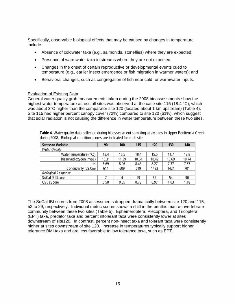
15
Specifically, observable biological effects that may be caused by changes in temperature include:
Absence of coldwater taxa (e.g., salmonids, stoneflies) where they are expected;
Presence of warmwater taxa in streams where they are not expected;
Changes in the onset of certain reproductive or developmental events cued to temperature (e.g., earlier insect emergence or fish migration in warmer waters); and
Behavioral changes, such as congregation of fish near cold- or warmwater inputs.
Evaluation of Existing Data General water quality grab measurements taken during the 2008 bioassessments show the highest water temperature across all sites was observed at the case site 115 (18.4 °C), which was about 3°C higher than the comparator site 120 (located about 1 km upstream) (Table 4). Site 115 had higher percent canopy cover (72%) compared to site 120 (61%), which suggest that solar radiation is not causing the difference in water temperature between these two sites.
Table 4. Water quality data collected during bioassessment sampling at six sites in Upper Penitencia Creek during 2008. Biological condition scores are indicated for each site.
Stressor Variable 90 100 115 120 130 140 Water Quality
Water temperature (°C) 13.4 16.5 18.4 15.5 11.7 12.8 Dissolved oxygen (mg/L) 10.31 11.39 10.54 10.42 10.69 10.74
pH 6.69 8.06 8.43 8.27 7.37 7.57 Conductivity (uS/cm) 614 609 619 1433 1424 701
Biological Response SoCal IBI Score 7 4 29 52 54 90 CSCI Score 0.58 0.55 0.78 0.97 1.03 1.18
The SoCal IBI scores from 2008 assessments dropped dramatically between site 120 and 115, 52 to 29, respectively. Individual metric scores shows a shift in the benthic macro-invertebrate community between these two sites (Table 5). Ephemeroptera, Plecoptera, and Tricoptera (EPT) taxa, predator taxa and percent intolerant taxa were consistently lower at sites downstream of site120. In contrast, percent non-insect taxa and tolerant taxa were consistently higher at sites downstream of site 120. Increase in temperatures typically support higher tolerance BMI taxa and are less favorable to low tolerance taxa, such as EPT.

16
Table 5. Raw metric scores used to calculate SoCal IBI scores at six bioassessment sites in Upper Penitencia Creek sampled in 2008.
Continuous water temperature data collected at six sites between April and September, 2013 are presented in Table 6. The highest mean water temperature (21 °C) across all sites was observed at site 114 (just upstream of site 115). The mean temperature at site 114 was nearly 4°C warmer than site 121. Table 6 inludes biological condition scores for three of the sites sampled in 2012 and 2013; bioassessments were not conducted at the comparator site in 2012 or 2013.
Table 6. Summary statistics of continuous water quality data collected at six locations in Upper Penitencia Creek between April and September, 2013. Biological condition scores are indicated for each site. Sites with no available bioassessment data are indicated as “NA”.
Temperature (°C) 105 114 121 130 140 142 Minimum 15.3 15.7 11.5 11.7 11.1 9.5
Median 20.4 21.0 17.4 17.9 15.7 16.2 Mean 20.4 21.0 17.3 18.1 15.7 16.1
Maximum 27.4 27.6 24.2 26.7 20.5 22.3 Max 7-day Mean 24.1 25.1 20.6 22.3 18.1 19.1 SoCal IBI Score 21 30 NA NA 99 NA
CSCI Score 0.67 0.72 NA NA 1.19 NA The combined grab sample and continuous water temperature data provide evidence supporting the conclusion that altered water temperature may be impacting the biological condition at site 114 and 115. It is important to note that both of these sites occur in the dryback zone, but are typically wet during part of the dry season due to augmented flow from the percolation pond (see next section). Conductivity was over two times the levels at comparator site compared to case site, indicating a major change in water chemistry likely occurs between the two sites.
Station Code 90 100 115 120 130 140 Sample Date 4/30/2008 4/30/2008 5/1/2008 5/1/2008 5/2/2008 5/2/2008
Raw
Metri
c
EPT Taxa 4 3 9 13 25 25 Number Coleoptera Taxa 0 0 1 2 7 7 Number Predator Taxa 4 4 9 10 15 15 Percent CF + CG Individuals 97 95 92 90 64 64 Percent Intolerant 0 0 1 7 28 28 Percent Non-Insecta Taxa 56 59 48 25 17 17 Percent Tolerant Taxa (8-10) 31 41 24 16 15 15
SoCal IBI Score 7 4 29 52 54 90

17
3.3.2 Altered Flow Regime Potential Impacts The channel flow regime, as characterized by water velocity, water depth, and water discharge patterns, can affect aquatic biota. The flow regime can be altered by human activities such as water management, construction of impervious surfaces, agriculture-related extraction and discharge, point source discharges, or industrial or mining extraction. Flow characteristics are regionally and temporally variable. Variance in rainfall patterns, vegetation, development, geology, and other characteristics of the landscape in the watershed results in natural variability of flow. Channel morphology also plays a role, with reach characteristics such as the presence of pools or riffles affecting local flow velocities. Biological characteristics can be affected by flow alteration through a variety of mechanisms (Figure 6). The volume, velocity, and variance of both low flows (baseflows or average flows) and high flows (peak or stormflows) affect which types of species are best able to survive. Changes in flow may harm some species and help others, resulting in changes to biotic community structure. For example, if water is abstracted, the magnitude of flow may decrease and low-flow duration will increase. This could lead to channel drying which in turn results in a greater abundance of drought-tolerant taxa. However, if runoff or other inputs increase, then the magnitude and duration of high flows will increase. This can result in scouring and displacement of biota and subsequent reduction in benthic taxa or life stages. Biological effects that may be caused by flow alteration include:
Reduced productivity
Changes in community composition
Increased generalists and decreased specialists
Replacement of native species by invasive or exotic species
Disrupted reproductive cycles
Decreased taxonomic richness and diversity Human activities can alter flow on a watershed scale, affecting discharge based on hydrologic variables, and at the reach scale, affecting local stream velocity based on hydraulic variables (Figure 6). These changes can be indirect, due to development or land use changes in the surrounding landscape, or direct, due to channel alteration, impoundments, or point source inputs and withdrawals. Removal of forest, vegetation, or development of the watershed causes increases in surface runoff, resulting in higher magnitudes and frequencies of peak discharges. Flow may also interact with other biological stressors such as temperature, physical habitat, dissolved oxygen, and sediment. If flow causes change in temperature or physical habitat, it may be considered a proximate cause of biological impairment. For example, urbanization and related watershed devegetation may reduce groundwater recharge resulting in lower groundwater coldwater inputs. This may cause or contribute to increases in temperature. Flow is also closely tied to physical habitat. Geomorphic features may be affected by many flow-related processes including scoring, sediment transport and deposition, and erosion.

18
Figure 6. Conceptual model for primary stressor of Flow Alteration (EPA 2010).

19
Evaluation of Existing Data Stream flow data are available from two gages, located at Dorel Road crossing (site 121) and Piedmont Road crossing (site 114). The Santa Clara Valley Water District (SCVWD) operates both stream gages. Stage heights and flow rates recorded at Dorel and Piedmont gages during 20132 are graphed in Figure 7. At the Dorel site, stream flow measured between mid-June and mid-September was generally < 0.1 cfs and for some periods, the channel appears to be dry. During the same time period, flow measured at Piedmont Road (approximately 1 km downstream of Dorel) was between 3 and 5 cfs. This increase in flow can be explained by releases from the percolation ponds just upstream of Piedmont Road. Thus stream flow was greater and more persistent at the case site versus the comparator site. Higher flow conditions from percolation pond discharges during the dry season would generally be associated with improved biological conditions. Augmented flows would likely support a native fish community in a reach that typically dries up during the summer. Lower BMI condition at the case site, however indicates that something other than altered stream flow (e.g., water quality) is impacting BMIs.
2 Flow data from both Piedmont and Dorel gages were not available prior to 2010.

20
Figure 7. Flow data recorded from from Dorel Drive (site 121) stream gage (upper figure) and Piedmont Av (site 114) stream gage (lower figure) during 2013.

21
3.3.3 Altered Physical Habitat Potential Impacts Physical habitat in the stream, as characterized by structural geomorphic or vegetative features of the channel, can also affect aquatic biota (Figure 8). Physical habitat can be affected by human activities that alter these features, such as the construction of in-stream or riparian man-made structures (e.g. dams, channelization) or the development of local areas affecting riparian vegetation or other stream habitat qualities. Physical habitat varies naturally and organisms are adapted to various stream conditions. Therefore, the quality of physical habitat is defined by its natural condition. The primary attributes of stream physical habitat are 1) Stream size and channel dimensions, 2) Channel gradient, 3) Channel substrate size and type, 4) Habitat complexity and cover, 5) Vegetation cover and structure in the riparian zone, and 6) Channel-riparian interactions. A high-quality stream habitat is likely to be characterized by the presence of riffles and pools in alternating sequence, stream channels that are unaltered (e.g. not incised or channelized), stream banks and riparian zones that are well-vegetated with native plants. Organisms may require specific habitat attributes for specific life stages or aquatic conditions. For example, during low flow periods fish may require deep pools for survival. Fish and macroinvertebrates rely on vegetation and deep pools in the channel as refugia from predators and competitors. High-quality physical habitat provides cover and diversity of substrate and hydraulic conditions to fulfill the various requirements of aquatic biota. Biological effects that may be caused by alteration of physical habitat include:
Reduced abundance of young-of-year fish
Reduced fish taxonomic richness
Reduced relative abundance of clinging and sprawling invertebrates
Changes in relative abundance of invertebrate functional feeding groups (e.g., grazers)
Changes in periphyton biomass and species composition. Human activity can alter any of the six attributes of stream habitat (Figure 8). Man-made structures in the stream such as dams, rip-rap, culverts, revetments, bridge abutments, and channelization are clear interruptions of natural physical habitat altering flow, erosion, and sediment deposition. They can pose barriers to migration and impede riparian habitat. Indirect anthropogenic factors affecting physical habitat include changes in watershed or riparian land uses that cause erosion or changes in stormwater runoff. These may be the result of urbanization or agricultural, industrial, forestry, or resource extraction practice.

22
Figure 8. Conceptual model for primary stressor of Physical Habitat Alteration (EPA 2010).

23
Data Evaluation The stressor variables related to physical habitat for 2008 bioassessment sites are presented in Table 7. The habitat variables did not provide a conclusive line of evidence for causing biological impact at the case site. The PHAB condition metrics epifaunal substrate and channel alteration scores were very similar between both sites (115 and 120). Mean substrate size was also similar between sites. However, site 120 had higher percent riffles, which would positively affect biological condition. However, site 120 also had higher percent sands and fine substrate, which would negatively affect biological condition. As a result, the existing physical habitat data does not conclusively indicate positive or negative line of evidence for impacts to the biological condition scores.
Table 7. Physical habitat collected during bioassessment sampling at six sites in Upper Penitencia Creek during 2008. Biological condition scores are indicated for each site.
Stressor Variable 90 100 115 120 130 140 Physical Habitat % Canopy Cover 62 65 72 61 51 46 % Sands & Fines 34.3 41.0 18.1 24.8 12.4 16.2 Mean Substrate Size (cm) 34.6 22.4 91.0 95.6 207.6 184.8 Epifaunal Substrate Score (0-20; 0: low; 20:high) 8 8 15 16 17 17 Channel Alterations Score (0-20; 0: low; 20:high) 6 10 16 17 14 19 % Pools 6 31 10 7 19 0 % Riffles 30 20 28 38 36 39 Biological Response SoCal IBI Score 7 4 29 52 54 90 CSCI Score 0.58 0.55 0.78 0.97 1.03 1.18
3.3.4 Low Dissolved Oxygen Potential Impacts In healthy aquatic ecosystems, oxygen becomes dissolved in the water column as it is absorbed from the atmosphere and released into the water column by aquatic plants during photosynthesis (Figure 9). This dissolved oxygen supports aquatic life including fish and invertebrates. However, if dissolved oxygen levels are severely depleted, fish and invertebrates may be impaired or killed. Large fluctuations in DO over a short period of time (i.e. daily) can also stress aquatic organisms. Urban and agricultural land uses can cause low DO through chemical, nutrient, and organic waste pollution or through the alteration of stream channels and riparian vegetation. Changes in aquatic community structure may be due to DO levels below that of healthy ecosystems. Species that are particularly sensitive to low DO include some species of mayflies, stoneflies, caddisflies, and beetles. Tolerant worms and fly larvae that are more tolerant to low DO may be able to out-compete these organisms when DO drops. When DO reaches acute low levels, the following biological effects may occur:
Kills of aquatic life especially
O species with highest oxygen demands
O large fish of certain species
O during the night/early morning hours
Fish gulping air and staying in shallow water

24
Body movements to increase water flow (e.g. stonefly larvae “push-ups” or caddisfly larvae undulating)
Abundance of decaying vegetation
Dead or dying zooplankters Many human activities can contribute to loss in dissolved oxygen in aquatic ecosystems through the reduction of natural aeration or the addition of chemical or biological oxygen demand (Figure 9). Some agricultural, forestry, and channel or steam alterations (e.g. channel straightening or creation of downstream impoundments) may reduce the aeration of water flowing through creeks and streams. In addition to this direct loss of aeration, particulate and dissolved materials that enter waterways through human activities can biologically or chemically convert oxygen, thereby decreasing its concentrations. This biological or chemical oxygen demand comes from nutrients, chemical contaminants, or organic matter, which may be released from municipal waste treatment plant overflows, septic seepage, and industrial point sources. Commonly, biological or chemical oxygen demand may enter streams as fertilizers or pesticides from agricultural and urban runoff. Devegetation of riparian areas can also play a role. Removing vegetation decreases shading, affecting temperatures and plants; DO production from aquatic plants increases in daylight hours, but oxygen demand increases during the night. Aquatic plant decomposition and reduction of woody debris from riparian trees or shrubs (reducing aeration) can also lead to depleted DO as a result of reduced riparian vegetation. DO can also interact with other stressors, primarily temperature, ionic strength, and sediments.

25
Figure 9. Conceptual model for primary stressor of Reduced Dissolved Oxygen (EPA 2010).

26
Data Evaluation Spot measurements of dissolved oxygen concentration at sites 115 and 120 during the 2008 bioassessments were 10.5 mg/L and 10.4 mg/L, respectively, suggesting that DO is not impacting the biological condition at the case site (see Table 4 in Section 3.3.1). Furthermore, these DO levels are not considered detrimental to biological condition for BMIs or fish communities. However, single grab sample measurement of DO does not provide conclusive evidence to support or not support the cause. Continuous water quality measurements collected at both the case and comparator sites would provide data to more conclusively evaluate this potential cause. 3.3.5 Nutrients Nutrients such as Nitrogen (N) and Phosphorus (P) are essential for plant growth and reproduction. The balance of nutrients available in the aquatic environment plays a role in limiting the growth rate of aquatic plants and algae (Figure 10). Commonly, when nutrient concentrations in waterways become too high, excess algal growth occurs, causing changes in fish and macroinvertebrate food resources and habitat structure. Additionally, algal toxins may be produced when nutrients lead to excessive algal growth. Through this process, nutrients entering waterways from point sources or runoff can indirectly cause harm to aquatic biological communities. A wide range of human activities can cause excessive nutrients to enter waterways. Point-source discharges containing high nutrient levels may be released from industrial or wastewater treatment plant effluents, combined sanitary sewer outfalls, or septic systems. Runoff may also carry nutrients from many sources in the watershed. These land-based nutrient sources include agricultural land, pasture or rangeland, animal feeding operations, landfills, landscaped areas (e.g. lawns, golf courses), impervious surfaces in urban/suburban areas, or construction and development sites. Changes in land use that result in changes to surface runoff or erosion can mobilize Nitrogen and Phosphorus, resulting in higher concentrations reaching waterways. Many factors interact with nutrient levels and resulting algal growth (Figure 10). Excessive algal growth may also be limited by factors such as available sunlight and may interact with other stressors such as dissolved oxygen (growth depletes oxygen), pH, and sediments. The proliferation of filamentous algae or algal mats, phytoplankton blooms, and abundant macrophytes are evidence of excessive nutrient concentrations that may be harming biological communities.

27
Figure 10. Conceptual model for primary stressor of Increased Nutrients (EPA 2010).

28
Data Evaluation Nutrient data was collected at site 105 in 2012 and sites 114 and 140 in 2013 (Table 8). A causal assessment for nutrients was inconclusive due to a lack of nutrient data from a comparator site. In general, concentrations for all nutrients at sites 105 and 114 were higher compared to site 140, which is located much further upstream of the comparator site. Additional nutrient data collected from both case and comparator sites are needed to assess potetnial correlations between BMIs and nutrients.
Table 8. Nutrient data collected during bioassessment sampling at site 105 in 2012 and at sites 115 (case site) and 140 in 2013
Stressor Variable 105 114 140 Monitoring Year 2012 2013 2013 Nutrients
Un-ionized ammonia (µg/L) 2.05 8.74 1.10 Ammonia as N (mg/L) 0.12 0.12 0.044 Chloride (mg/L) 46 54 16 Dissolved Organic Carbon (mg/L) 4.2 4.5 2.2 Nitrate as N (mg/L) 0.33 0.37 0.096 Nitrite as N (mg/L) 0.001 0.002 0.001 Nitrogen, Total Kjeldahl (mg/L) 0.44 0.59 0.13 OrthoPhosphate as P (mg/L) 0.072 0.1 0.034 Phosphorus as P (mg/L) 0.087 0.11 0.027 Chlorophyll a (mg/m2) 68.6 70.4 6.9 Ash Free Dry Mass (g/m2) 213 126.7 42.2 Biological Response
SoCal IBI Score 21 30 99 CSCI Score 0.67 0.72 1.19 Diatom IBI Score 48 58 66
Nutrient data and bioassessment data are presented in Table 8. It is important to note that increased nutrients are not expected to directly impact BMIs (i.e., nutrients are not the proximate stressor), making it difficult to assess relationships between nutrients and BMIs. Effects from nutrients may alter primary production (i.e., biomass) which may in turn impact BMI composition. An increase in algal biomass may especially occur in the percolation ponds, where sunlight exposure is dramatically increased compared to stream conditions. Algae diatom IBI scores could be used as a more direct measure of the effects of nutrients on biological communities. Interpretative tools for algal data, developed for Southern California creeks, are being tested in other ecological regions in California (Fetscher et al. 2013). Specifically, the “H20” hybrid IBI (Algae IBI), which combines eight metrics that measure both diatom and soft algae community assemblage, had the greatest performance for detecting changes in nutrient concentrations. Nutrient concentrations will be compared to Algal IBI scores, as well as the chlorophyll a and ash free dry weight concentrations, both analytes generated from the benthic algae samples.

29
3.3.6 Insecticides Potential Impacts Insecticides bound to sediments or dissolved in the water column can be harmful to aquatic organisms (Figure 11). Bioaccumulation of pesticides may occur as small organisms transfer larger concentrations of insecticides to their predators, consequently affecting the aquatic community and ecosystem. Insecticides applied in agricultural or urban areas can enter waterways through stormwater or irrigation runoff. Even if concentrations in the water column of a stream are below detection, insecticides bound to sediments or occurring in episodic patterns from temporally varying sources (e.g. storm events) may yet be affecting aquatic biota. The toxicity of insecticides may be influenced by local water quality characteristics such as dissolved organic carbon or suspended sediment and temperature or by interactions with other pollutants. Possible biological effects of increased insecticides in stream water or sediment include:
Decreased biological condition
Decreased growth
Altered behavior
Increased susceptibility to other stressors
Increased mortality
Decreased reproductive success in affected biota
Altered population and community structure Because of the prevalence of Pyrethroids in urban insecticide applications and its existence in Bay Area waterways (SCVURPPP 2013), this insecticide type is a more likely candidate stressor than other types. Extremely toxic to fish, Pyrethroids function “by keeping open the sodium channels in neuronal membranes affecting both the peripheral and central nervous systems causing a hyper-excitable state causing such symptoms as tremors, incoordination, hyperactivity, and paralysis” (USEPA 2010).

Preliminary Draft – Do Not Cite or Distribute
30
Figure 11. Conceptual model for primary stressor of Increased Insecticides (EPA 2010).

Preliminary Draft – Do Not Cite or Distribute
31
Data Evaluation Existing sediment chemistry data and water and sediment toxicity testing conducted on samples collected at site 105 in 2012 indicate that pesticides and metals were not present in concentrations that are toxic to aquatic life uses (SCVURPPP 2013). Although no data are available from the case or comparator sites, available data suggest that pesticides or metals were not present in concentrations to impact biological conditions at site 105, approximately one mile further downstream of the case site. That said, pesticide-related impacts are episodic and are known to cause toxicity in creeks in the Bay Area and throughout California, suggesting that pesticides could be a causal factor of reduced biological integrity in Upper Penitencia Creek. 3.4 Preliminary Evaluation of Probable Causes Existing data sources used to evaluate each of the candidate causes is presented in Table 9. The quality of existing data sources for spatial temporal co-occurrence evaluation of the candidate causes is provided, as well as information gaps. Table 9 also shows a preliminary assessment of probably causes for impact at the case site. Table 9. Data quality assessment for evaluation of the candidate causes.
Causal Factor
Evidence Type Spatial/Temporal Co-occurrence
Evidence
Probable Cause Data Type Indicator Conclusions
Physical Habitat; Sedimentation
PHAB PHAB score; % fines+sands Yes, only for 2008 Similar habitat conditions; no
clear correlations Unknown
Reduced Dissolved Oxygen
General WQ DO concentration Yes, only for 2008 DO levels not problematic for
life uses; grab samples only Unlikely
Increased Nutrients Nutrients N and P
chl a, AFDM No (case only) Nutrients may impact benthic
algae. Impacts to BMIs unclear
Unknown
Pesticides and Metals
Sediment Chemistry
Metals; Pyrethroids
No (case only) Pesticide levels at site just below case site; No toxicity
observed Unknown
Toxicity Testing % survival
Increased Temperature
Temperature Logger Mean ⁰C Yes (not synoptic
with bioassessment) Approximate 4 C increase
below ponds Likely
Altered Flow Regime
Flow gage or velocity
Stream discharge (cfs)
Yes (not synoptic with bioassessment)
Higher flow at impacted site; however, altered flow may
result in change to BMI Unknown
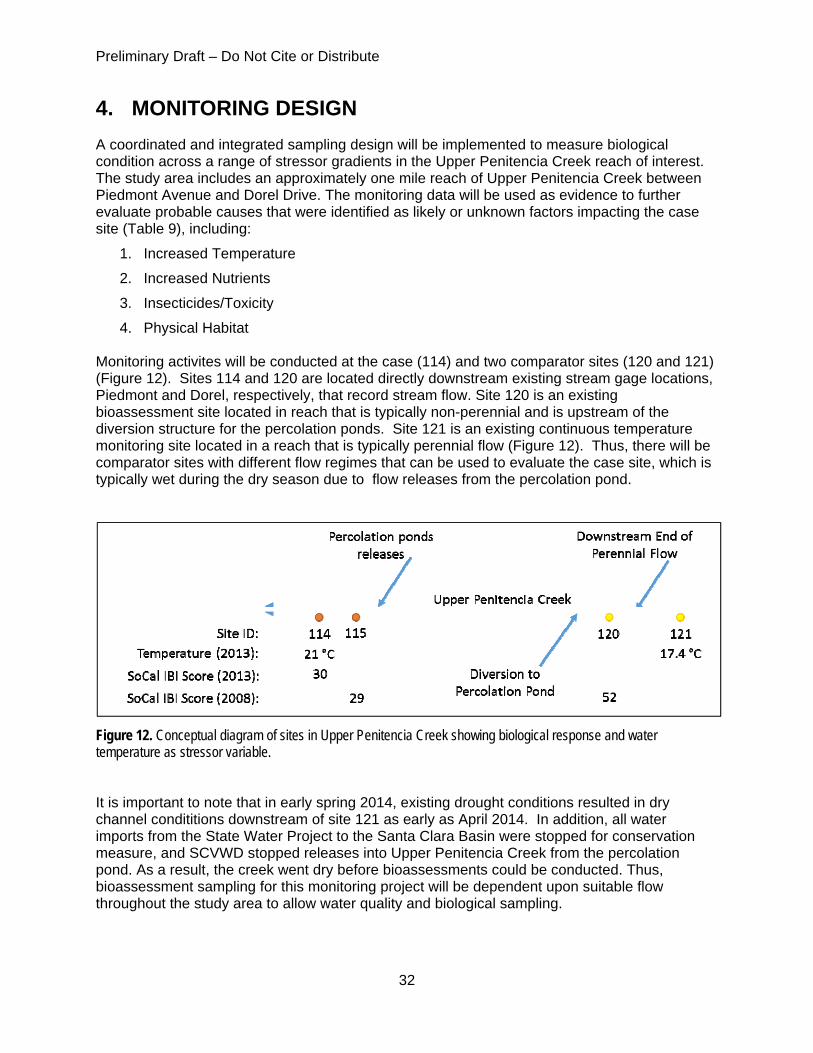
Preliminary Draft – Do Not Cite or Distribute
32
4. MONITORING DESIGN A coordinated and integrated sampling design will be implemented to measure biological condition across a range of stressor gradients in the Upper Penitencia Creek reach of interest. The study area includes an approximately one mile reach of Upper Penitencia Creek between Piedmont Avenue and Dorel Drive. The monitoring data will be used as evidence to further evaluate probable causes that were identified as likely or unknown factors impacting the case site (Table 9), including:
1. Increased Temperature
2. Increased Nutrients
3. Insecticides/Toxicity
4. Physical Habitat Monitoring activites will be conducted at the case (114) and two comparator sites (120 and 121) (Figure 12). Sites 114 and 120 are located directly downstream existing stream gage locations, Piedmont and Dorel, respectively, that record stream flow. Site 120 is an existing bioassessment site located in reach that is typically non-perennial and is upstream of the diversion structure for the percolation ponds. Site 121 is an existing continuous temperature monitoring site located in a reach that is typically perennial flow (Figure 12). Thus, there will be comparator sites with different flow regimes that can be used to evaluate the case site, which is typically wet during the dry season due to flow releases from the percolation pond.
Figure 12. Conceptual diagram of sites in Upper Penitencia Creek showing biological response and water temperature as stressor variable. It is important to note that in early spring 2014, existing drought conditions resulted in dry channel condititions downstream of site 121 as early as April 2014. In addition, all water imports from the State Water Project to the Santa Clara Basin were stopped for conservation measure, and SCVWD stopped releases into Upper Penitencia Creek from the percolation pond. As a result, the creek went dry before bioassessments could be conducted. Thus, bioassessment sampling for this monitoring project will be dependent upon suitable flow throughout the study area to allow water quality and biological sampling.

Preliminary Draft – Do Not Cite or Distribute
33
4.1 Sampling Location and schedule The study area includes a one mile section of Upper Penitencia Creek between Piedmont Av and Dorel Drive. Monitoring activities would occur between April and July 2015. Monitoring parameters, sampling frequency and location are presented in Table 10 and illustrated in Figure 13. Stormdrain network and percolation outfall are also indicated in Figure 13. The monitoring period may get moved to late March if minimal flows are present due to lack of rainfall.
Table 10. Parameter, frequency and location of monitoring in spring/summer season of 2015.
Monitoring Parameter Frequency and Timing
Sample Location 114 120 121
Piedmont Toyon Dorel Bioassessment
1x – April/May
BMI x x x
Algae x x x Physical Habitat x x x Nutrients x x Sediment Toxicity and pesticides
1x – April/May x x
Continuous Temperature April - July x x x Continuous Water Quality (DO, pH, conductivity)
2 weeks prior to bioassessment x x
Figure 13. Monitoring locations in Upper Penitencia Creek for 2015.

Preliminary Draft – Do Not Cite or Distribute
34
4.2 Sampling methods The sampling methods used for this project will be consistent with methods used by SCVURPPP for the RMC Creek Status Monitoring Project (BASMAA 2014). A summary of these methods is provided below. 4.2.1 Benthic Macroinvertebrates Each bioassessment sampling site will consist of an approximately 150-meter stream reach divided into 11 equidistant transects placed perpendicular to the direction of flow. The sampling position within each transect will alternate between 25%, 50% and 75% distance of the wetted width of the stream. Benthic macroinvertebrates (BMIs) will be collected from a 1 square foot area approximately 1 m downstream of each transect (Ode 2007). The benthos are disturbed by manually rubbing coarse substrate followed by disturbing the upper layers of substrate to a depth of 4-6 inches to dislodge any remaining invertebrates into the net. Material collected from the eleven subsamples will be composited in the field by transferring the entire sample into one or two 1000 ml wide-mouth jar(s) and preserving it with 95% ethanol. 4.2.2 Algae Filamentous algae and diatoms will be collected using the Reach-Wide Benthos (RWB) method (Fetscher et al 2009). Algae samples will be collected synoptically with and immediately after BMI sample collection. The sampling position within each transect is the same as used for BMI sampling; however, samples are collected six inches upstream of the BMI sampling position. The algae will be collected using a range of methods and equipment, depending on the particular substrate occurring at the site (i.e., erosional, depositional, large and/or immobile, etc.). Erosional substrates included any material (substrate or organics) small enough to be removed from the stream bed, but large enough in size to isolate an area equal in size to a rubber delimiter (12.6 cm2 in area). When a sample location along a transect is too deep to sample, a more suitable location will be selected, either on the same transect or from one further upstream. Algae samples will be collected at each transect prior to moving on to the next transect. Sample material (substrate and water) from all eleven transects is combined in a sample bucket, agitated, and a suspended algae sample was then poured into a 500 mL cylinder, creating a composite sample for the site. A 45 mL subsample is taken from the algae composite sample and combined with 5 mL glutaraldehyde into a 50 mL sample tube for taxonomic identification of soft algae. Similarly, a 40 mL subsample is extracted from the algae composite sample and combined with 10 mL of 10% formalin into a 50 mL sample tube for taxonomic identification of diatoms. Laboratory processing will include identification and enumeration of 300 natural units of soft algae and 600 diatom valves to the lowest practical taxonomic level. The algae composite sample will be used for the collection of chlorophyll a and ash free dry mass (AFDM) samples following methods described in Fetscher et al (2009). For the chlorophyll a sample, 25 mL of the algae composite volume is removed and run through a glass fiber filter (47 mm, 0.7 um pore size) using a filtering tower apparatus. The AFDM sample is collected using a similar process using pre-combusted filters. Both samples are placed in whirlpaks, covered in aluminum foil and immediately placed on ice for transportation to laboratory.

Preliminary Draft – Do Not Cite or Distribute
35
4.2.3 Physical Habitat Physical habitat assessments (PHAB) will be conducted at each BMI bioassessment sampling site using the PHAB protocols described in Ode (2007). Physical habitat data is collected at each of the 11 transects and at 10 additional inter-transects (located between each main transect) by implementing the “Basic” level of effort, with the following additional measurements/assessments as defined in the “Full” level of effort: water depth and pebble counts, cobble embeddedness, flow habitat delineation, and instream habitat complexity. At algae sampling locations, additional assessment of presence of micro- and macroalgae is conducted during the pebble counts. In addition, water velocities were measured at a single location in the sample reach (when possible) using protocols described in Ode (2007). 4.2.4 Physico-chemical Measurements General water quality parameters (dissolved oxygen, temperature, specific conductivity, and pH) will be measured concurrent with BMI bioassessment sampling using multi-parameters probes. Direct field measurements or grab samples for field measurement purposes will be collected from a location where the stream visually appears to be completely mixed. Ideally this is at the centroid of the flow, but site conditions do not always allow centroid collection. Measurements should occur upstream of sampling personnel and equipment and upstream of areas where bed sediments have been disturbed, or prior to such bed disturbance. Field meters will be calibrated prior to use and results are recorded on the Field Meter Calibration Record form. 4.2.5 Nutrients and Conventional Analytes Water samples will be collected at sites for nutrients and conventional analytes using the Standard Grab Sample Collection Method (BASMAA 2014). Sample containers are rinsed using ambient water and completely filled and recapped below water surface whenever possible. An intermediate container is used to collect water for all sample containers with preservative already added in advance by the laboratory. A syringe filtration method is used to collect samples for analyses of Dissolved Ortho-Phosphate and Dissolved Organic Carbon. All sample containers will be labeled and stored on ice for transportation to laboratory. 4.2.6 Sediment Toxicity and Chemistry Sediment samples will be collected at sites for toxicity and chemical analysis. Field personnel will survey the sampling area for appropriate fine-sediment depositional areas before stepping into the stream, to avoid disturbing possible sediment collection sub-sites. Personnel will carefully enter the stream and sampling at the closest appropriate reach, continuing upstream. Sediment samples will be collected from the top 2 cm of sediment in a compositing container, thoroughly homogenized, and then aliquotted into separate jars for chemical or toxicological analysis using standard clean sampling techniques. 4.2.7 Continuous Temperature Monitoring Digital temperature loggers (Onset HOBO Water Temp Pro V2) will be programmed to record data at 60-minute intervals. Procedures used for calibrating, deploying, programming and downloading data are described in BASMAA (2014). 4.2.8 Continuous General Water Quality Measurements Water quality monitoring equipment recording dissolved oxygen, temperature, conductivity, and pH at 15-minute intervals (YSI 6600 data sondes) will be deployed for two 2-week period prior to

Preliminary Draft – Do Not Cite or Distribute
36
the bioassessment sampling event. Procedures used for calibrating, deploying, programming and downloading data are described in BASMAA (2014). 5. REFERENCES Bay Area Stormwater Management Agency Association (BASMAA) Regional Monitoring
Coalition. 2014. Creek Status Monitoring Program Standard Operating Procedures. Version 2.0. Prepared for BASMAA by EOA, Inc. on behalf of the Santa Clara Urban Runoff Pollution Prevention Program and the San Mateo Countywide Water Pollution Prevention Program, Applied Marine Sciences on behalf of the Alameda Countywide Clean Water Program, and Armand Ruby Consulting on behalf of the Contra Costa Clean Water Program. 196 pp.
Beller E.E., Grossinger R.M., Nicholson M., and Salomon M.N. 2012. Upper Penitencia Creek Historical Ecology Assessment. A report of SFEI’s Historical Ecology Program, SFEI Publication #664, San Francisco Estuary Institute, Richmond, CA.
Fetscher, A.E, L. Busse, and P.R. Ode. 2009. Standard Operating Procedures for Collecting Stream Algae Samples and Associated Physical Habitat and Chemical Data for Ambient Bioassessments in California. California State Water Resources Control Board Surface Water Ambient Monitoring Program (SWAMP) Bioassessment SOP 002. (Updated May 2010).
Fetscher, A.E., M.A. Sutula, L.B. Busse and E.D. Stein. 2013. Condition of California Perennial, Wadeable Streams Based on Algal Indicators. Final Technical Report 2007-11. Prepared by Southern California Coastal Water Research Project and San Diego Regional Water Quality Control Board. Prepared for California State Water Board.
Mazor, R.D., A. Rehn, P.R. Ode, M. Engeln, K. Schiff, E. Stein, D. Gillet, D. Herbst, and C.P. Hawkins. (in review). Bioassessment in complex environments: Designing an index for consistent meaning in different settings.
Ode, P.R., A. Rehn, and J. May. 2005. Quantitative Tool for Assessing the Integrity of Southern Coastal California Streams, Environmental Management Vol. 35, No. 4, pp. 493-504.
Ode, P.R. 2007. Standard Operating Procedures for Collection Macroinvertebrate Samples and Associated Physical and Chemical Data for Ambient Bioassessments in California. California State Water Resources Control Board Surface Water Ambient Monitoring Program (SWAMP) Bioassessment SOP 001.
Santa Clara Valley Urban Runoff Pollution Prevention Program (SCVURPPP). 2008. Watershed Monitoring and Assessment Summary Report: Coyote Creek and Lower Penitencia Creek. Submitted in fulfillment of NPDES permit provision C.10 (b), Sunnyvale, California. September 15, 2008.
Santa Clara Valley Urban Runoff Pollution Prevention Program (SCVURPPP). 2013. Program Annual Report FY 2012-2013. Section 9: Pesticide Toxicity Control. Appendix 9-1: Pesticide Source Control Effectiveness Evaluation. September 15, 2013.
Santa Clara Valley Urban Runoff Pollution Prevention Program (SCVURPPP). 2014. Appendix A. Creek Status Monitoring Report. Water Years 2012 and 2013 (October 2011 – September 2013). Submitted in fulfillment of Provision C.8.g.v of NPDES Permit # CAS612008. March 15, 2014.

Preliminary Draft – Do Not Cite or Distribute
37
Stillwater Sciences. 2006. Upper Penitencia Creek Limiting Factors Analysis, Final Report. Prepared for Santa Clara Valley Urban Runoff Pollution Prevention Program (Program Managers, EOA, Inc.). 72 pp plus figures and appendices.
U.S. EPA (Environmental Protection Agency). 2010. Causal Analysis/Diagnosis Decision Information System (CADDIS). Office of Research and Development, Washington, DC. Available online at http://www.epa.gov/caddis. Last updated September 23, 2010.

SCVURPPP Urban Creeks Monitoring Report
Appendix C POC Loads Monitoring Progress Report, Water Years 2012, 2013, and 2014

2014 PROGRESS REPORT
1
Pollutants of concern (POC) loads monitoring progress report, water years (WYs) 2012, 2013, and 2014
Prepared by
Alicia Gilbreath, Jennifer Hunt, Jing Wu, Patrick Kim, and Lester McKee
San Francisco Estuary Institute, Richmond, California
On
January 20, 2015
For
Bay Area Stormwater Management Agencies Association (BASMAA)
And
Regional Monitoring Program for Water Quality in San Francisco Bay (RMP) Sources Pathways and Loadings Workgroup (SPLWG) Small Tributaries Loading Strategy (STLS)

2014 PROGRESS REPORT
2
Acknowledgements
We appreciate the support and guidance from members of the Sources, Pathways and Loadings Workgroup of the Regional Monitoring Program for Water Quality in San Francisco Bay. The detailed work plan behind this work was developed through the Small Tributaries Loading Strategy (STLS) during a series of meetings in the summer of 2011. Local members on the STLS at that time were Arleen Feng, Lucy Buchan, Khalil Abusaba, Jamison Crosby, and Chris Sommers (for BASMAA); and Richard Looker, Jan O’Hara, and Tom Mumley (for the Water Board). Project assistance during planning and implementation of the field components was also provided by ADH Environmental (Lower Marsh Creek and San Leandro Creek), Balance Hydrologics (Guadalupe River), and Kinnetic Laboratories, Inc. (Pulgas Creek South) as contractors for ACCWP, CCCWP, SCVURPPP and SMCWPPP respectively. SFEI field and logistical support over the three-year project was provided by David Gluchowski, Emily Novick, April Robinson, Patrick Kim, Don Yee, and Rachel Eastman. SFEI’s data management team is acknowledged for their diligent delivery of quality assured well-managed data. Over the three-year duration of this project, this team included: Cristina Grosso, Amy Franz, John Ross, Don Yee, Adam Wong, and Michael Weaver. Pete Wilde (ADH Environmental), Chris Sommers, Bonnie DeBerry, and Lisa Sabin (EOA Inc.), and Arleen Feng (ACCWP) provided helpful written reviews of this report. This project was completed with funding provided by the Bay Area Stormwater Management Agencies Association (BASMAA) and the Regional Monitoring Program for Water Quality in San Francisco Bay (RMP).
This progress report can be cited as:
Gilbreath, A.N., Hunt, J.A., Wu, J., Kim, P.S., and McKee, L.J., 2015. Pollutants of concern (POC) loads monitoring progress report, water years (WYs) 2012, 2013, and 2014. A technical report prepared for the Regional Monitoring Program for Water Quality in San Francisco Bay (RMP), Sources, Pathways and Loadings Workgroup (SPLWG), Small Tributaries Loading Strategy (STLS). Contribution No. 741. San Francisco Estuary Institute, Richmond, California.

2014 PROGRESS REPORT
3
Table of contents
1. Introduction ...................................................................................................................................... 5
2. Field methods ................................................................................................................................... 6
2.1. Watershed physiography, sampling locations, and sampling methods ................................... 6
2.2. Loads computational methods ............................................................................................... 10
3. Continuous data quality assurance ................................................................................................. 13
3.1. Continuous data quality assurance methods .......................................................................... 13
3.2. Continuous data quality assurance summary ......................................................................... 14
4. Laboratory analysis and quality assurance ..................................................................................... 18
4.1. Sample preservation and laboratory analysis methods ......................................................... 18
4.2. Quality assurance methods for pollutants of concern concentration data ............................ 22
4.2.1. Holding Times ...................................................................................................................... 22
4.2.2 Sensitivity ............................................................................................................................ 22
4.2.3 Blank Contamination ........................................................................................................... 22
4.2.4 Precision .............................................................................................................................. 22
5 Results ............................................................................................................................................. 24
5.2 Project Quality Assurance Summary ....................................................................................... 24
5.3 Climate and flow at the sampling locations during water years 2012, 2013, and 2014 ......... 31
5.4 Concentrations of pollutants of concern during sampling to-date ........................................ 33
5.5 Loads of pollutants of concern computed for each sampling location................................... 37
5.5. Comparison of regression slopes and normalized loads estimates between watersheds ..... 39
6. Conclusions and next steps ............................................................................................................. 41
6.1. Current and future uses of the data ....................................................................................... 41
6.2. What data gaps remain at current loads stations? ................................................................. 42
6.3. Next Steps ............................................................................................................................... 45
7. References ...................................................................................................................................... 46
8. Detailed information for each sampling location ........................................................................... 56
8.1. Marsh Creek ............................................................................................................................ 56
8.2. North Richmond Pump Station ............................................................................................... 64
8.3. San Leandro Creek .................................................................................................................. 71
8.3. Guadalupe River .................................................................................................................... 81

2014 PROGRESS REPORT
4
8.3. Sunnyvale East Channel .......................................................................................................... 90
8.6. Pulgas Creek South Pump Station ......................................................................................... 100
Atachment 1. Quality Assurance information ...................................................................................... 109
Attachment 2. Intercomparison Studies ........................................................................................... 131
Trace Elements .................................................................................................................................. 132
Copper ............................................................................................................................................... 132
Total Mercury .................................................................................................................................... 133
Methylmercury ................................................................................................................................. 134
Selenium ........................................................................................................................................... 135
Hardness ........................................................................................................................................... 136
Suspended Sediment Concentration ................................................................................................ 137
Nutrients ........................................................................................................................................... 138
Pyrethroids ........................................................................................................................................ 141

2014 PROGRESS REPORT
5
1. Introduction The San Francisco Regional Water Quality Control Board (Water Board) has determined that San Francisco Bay is impaired by mercury and PCBs due to threats to wildlife and human consumers of fish from the Bay. These contaminants persist in the environment and accumulate in aquatic food webs (SFRWRCB 2006; SFRWRCB, 2008). The Water Board has identified urban runoff from local watersheds as a pathway for pollutants of concern into the Bay, including mercury and PCBs. The Municipal Regional Stormwater Permit (MRP; SFRWRCB, 2009) contains several provisions requiring studies to measure local watershed loads of suspended sediment (SS), total organic carbon (TOC), polychlorinated biphenyl (PCB), total mercury (HgT), total methylmercury (MeHgT), nitrate-N (NO3), phosphate-P (PO4), and total phosphorus (TP) (provision C.8.e), as well as other pollutants covered under provision C.14. (e.g. legacy pesticides, PBDEs, and selenium).
Four Bay Area Stormwater Programs1, represented by the Bay Area Stormwater Management Agencies Association (BASMAA), collaborated with the San Francisco Bay Regional Monitoring Program (RMP) to develop an alternative strategy allowed by Provision C.8.e of the MRP, known as the Small Tributaries Loading Strategy (STLS) (SFEI, 2009). An early version of the STLS provided an initial outline of the general strategy and activities to address four key management questions (MQs) that are found in MRP provision C.8.e:
MQ1. Which Bay tributaries (including stormwater conveyances) contribute most to Bay impairment from POCs;
MQ2. What are the annual loads or concentrations of POCs from tributaries to the Bay; MQ3. What are the decadal-scale loading or concentration trends of POCs from small tributaries to the Bay; and, MQ4. What are the projected impacts of management actions (including control measures) on tributaries and where should these management actions be implemented to have the greatest beneficial impact.
Since then, a Multi-Year-Plan (MYP) has been written (BASMAA, 2011) and updated twice (BASMAA, 2012; BASMAA, 2013). The MYP provides a comprehensive description of activities that will be implemented over the next 5-10 years to provide information and comply with the MRP. The MYP provides rationale for the methods and locations of proposed activities to answer the four MQs listed above. Activities include modeling using the regional watershed spreadsheet model (RWSM) to estimate regional scale loads (Lent and McKee, 2011; Lent et al., 2012; McKee et al., 2014), and pollutant characterization and loads monitoring in local tributaries beginning Water Year (WY) 2011 (McKee et al.,
1 Alameda Countywide Clean Water Program, Contra Costa Clean Water Program, San Mateo Clean Water Pollution Prevention Program and Santa Clara Urban Runoff Pollution Prevention Program conduct monitoring and other activities on behalf of MRP Permittees in the four largest Bay Area counties.

2014 PROGRESS REPORT
6
2012), that continued in WY 2012 (McKee et al., 2013), WY 2013 (Gilbreath et al., 2014), and was largely completed in WY 2014 (this report).
The purpose of this report is to describe data collected during all three WYs (2012, 2013, and 2014) in compliance with MRP provision C.8.e., following the standard report content described in provision C.8.g.vi. The study design (selected watersheds and sampling locations, analytes, sampling methodologies and frequencies) as outlined in the MYP was developed to assess concentrations and loads in watersheds that are considered to likely be important watersheds in relation to sensitive areas of the Bay margin (MQ1):
• Lower Marsh Creek (Hg); • North Richmond Pump Station (Hg and PCBs); • San Leandro Creek below Chabot dam (Hg); • Guadalupe River (Hg and PCBs); • Sunnyvale East Channel (PCBs); and • Pulgas Creek Pump Station South (PCBs).
Loads monitoring provides verification data for the RWSM (MQ2), and is intended to provide baseline data to assess long term loading trends (MQ3) in relation to management actions (MQ4). This report was structured to allow annual updates after each subsequent winter season of data collection. It should be noted that the sampling design described in this report (and modeling design: Lent and McKee, 2011; Lent et al., 2012; McKee et al., 2014) was focused mainly on addressing MQ2. During the next permit term (perhaps beginning in 2015), there will be an increasing focus towards finding high leverage watersheds and source areas within watersheds (MQ 1) for management focus (MQ4). A parallel report (the “POC synthesis report” (SFEI in preparation)) is intended to document progress to date towards addressing management questions and the rationale for changed monitoring design going forward that more carefully addresses MQ1 and MQ4.
2. Field methods
2.1. Watershed physiography, sampling locations, and sampling methods The San Francisco Bay estuary is surrounded by nine highly urbanized counties with a total population greater than seven million people (US Census Bureau, 2010). Although urban runoff from upwards of 300 small tributaries (note the number is dependent upon how the areas are lumped or split) flowing from the adjacent landscape represents only about 6% of the total freshwater input to the San Francisco Bay, this input has broadly been identified as a significant source of pollutants of concern (POCs) to the estuary (Davis et al., 2007; Oram et al., 2008; Davis et al., 2012; Gilbreath et al., 2012). Four watershed sites were sampled in WY 2012 and two additional watershed sites were added in WY 2013 and WY 2014 (Figure 1; Table 1). The sites were distributed throughout the counties where load monitoring was required by the MRP. The selected watersheds include areas with urban and industrial land uses, watersheds where stormwater programs are planning enhanced management actions to reduce PCB and mercury discharges, and watersheds with historic mercury or PCB occurrences or related management concerns.

2014 PROGRESS REPORT
7
Figure 1. Water year 2012, 2013 and 2014 sampling watersheds.

2014 PROGRESS REPORT
8
Table 1. Sampling locations in relation to Countywide stormwater programs and sampling methods at each site.
County program
Watershed name
Water years
sampled
Watershed area (km2)1
Sampling location
Operator Discharge
monitoring method
Turbidity
Water sampling for pollutant analysis
City Latitude (WGS1984)
Longitude (WGS1984)
Hg/MeHg collection
Discrete samples
excluding Hg species
Composite samples
Contra Costa
Marsh Creek 2012-2014 99 Brentwood 37.990723 -122.16265 ADH
USGS Gauge Number:
113376002;
STLS creek stage applied to USGS discharge rating
OBS-5004 Manual grab
ISCO auto pump
sampler8
ISCO auto pump
sampler8
Contra Costa
North Richmond
Pump Station
2013-2014 2.0 Richmond 37.953945 -122.37398 SFEI
Measurement of pump rotations/ interpolation of
pump curve
OBS-5004 FISP US D957
ISCO auto pump
sampler8
ISCO auto pump
sampler8
Alameda San Leandro Creek 2012-2014 8.9 San
Leandro 37.726073 -122.16265 SFEI WY2012
ADH WYs 2013-14
STLS creek stage/ velocity/ discharge
rating
OBS-500**4
FISP US D957 WY
2012 ISCO pump sampler WY
2013-14
ISCO auto pump
sampler8
ISCO auto pump
sampler8
Santa Clara
Guadalupe River 2012-2014 236 San Jose 37.373543 -121.69612
SFEI WY2012 Balance WYs
2013-14
USGS Gauge Number:
111690253 DTS-125 FISP US
D956 FISP US D956
FISP US D956
Santa Clara
Sunnyvale East
Channel 2012-2014 14.8 Sunnyvale 37.394487 -122.01047 SFEI
STLS creek stage applied to SCVWD discharge rating6
OBS-500*4
WY 2012 DTS-125
WYs 2013-14
FISP US D958
ISCO auto pump
sampler8
ISCO auto pump
sampler8
San Mateo
Pulgas Creek South
Pump Station9
2013-2014 0.6 San Carlos 37.504583 -122.24901 KLI
ISCO area velocity flow meter with an
ISCO 2150 flow module
DTS-125 Pole sampler
ISCO auto pump
sampler8
ISCO auto pump
sampler8 1Area downstream from reservoirs
2USGS 11337600 MARSH C A BRENTWOOD CA 3USGS 11169025 GUADALUPE R ABV HWY 101 A SAN JOSE CA 4Campbell Scientific OBS-500 Turbidity Probe
5Forest Technology Systems DTS-12 Turbidity Sensor 6This rating curve was verified with discharge velocity measurements in WY 2012 7FISP US D-95 Depth integrating suspended hand line sampler 8Teledyne ISCO 6712 Full Size Portable Sampler 9Both the northern and southern catchments to the Pulgas Creek Pump Station were sampled in the WY 2011 characterization study (McKee et al., 2012) *OBS-500 malfunctioned during WY 2012 due to low flow water depth. A DTS-12 was installed during WY 2013 **OBS-500 malfunctioned during some WY2014 events

FINAL PROGRESS REPORT
9
The monitoring design focused on winter season storms between October 1 and April 30 of each water year; the period when the majority of pollutant transport occurs in the Bay Area (McKee et al., 2003; McKee et al., 2006; Gilbreath et al, 2012). At all six sampling locations, measurement of continuous stage and turbidity at time intervals of 15 min or less was the basis of the chosen monitoring design (Table 1). At free flowing sites, stage was used along with a collection of discrete velocity measurements to generate a rating curve between stage and instantaneous discharge. Subsequently this rating curve was used to estimate a continuous discharge record over the wet season by either the STLS team or USGS depending on the sampling location (Table 1). At Richmond pump station, an optical proximity sensor (Omron, model E3F2) was used along with stage measurements and a pump efficiency curve based on the pump specifications to estimate flow. ISCO flow meters were deployed at the Pulgas Creek Pump Station (Table 1). Turbidity is a measure of the “cloudiness” in water caused by suspension of particles, most of which are less than 62.5 µm in size and, for most creeks in the Bay Area, virtually always less than 250 µm (McKee et al., 2003). In natural flowing rivers and urban creeks or storm drains, turbidity usually correlates with the concentrations of suspended sediments and hydrophobic pollutants. In the creek and channel sampling locations, turbidity probes were mounted in the thalweg of each sampling location on an articulated boom that allowed turbidity sampling at approximately mid-depth under most flow conditions (McKee et al., 2004). At North Richmond Pump Station, the turbidity probe was mounted on a boom that extended into the center of the central well. At Pulgas Creek South Pump Station, the turbidity probe was attached to the catch basin wall at a fixed height, which was selected to ensure the probe remained submerged.
Composite and discrete samples were collected for multiple analytes from the water column over the rising, peak, and falling stages of the hydrograph. The sampling design was developed to support the use of turbidity surrogate regression (TSR) during loads computations. This method is deemed one of the most accurate methods for the computation of loads of pollutants transported dominantly in particulate phase such as suspended sediments, mercury, PCBs and other pollutants (Walling and Webb, 1985; Lewis, 1996; Quémerais et al., 1999; Wall et al., 2005; Ruzycki et al., 2011; Gilbreath et al., 2012; Riscassi and Scanlon, 2013). The method involves logging a continuous turbidity record in a short time interval (15 min or less during the study) and collecting a number of discrete samples to support the development of pollutants specific regressions. In this study, although not always achievable (see discussion later in the report), field crews aimed to collect 16 samples per water year during an early storm, several mid-season storms (ideally including one of the largest storms of the season) and later season storm. The use of turbidity surrogate regression and the other components of this sampling design was recommended over a range of alternative designs (Melwani et al 2010), and was adopted by the STLS (BASMAA, 2011).
Discrete samples for analytes used for loads computations (except water samples collected for mercury, methylmercury and a simultaneously collected sample for suspended sediment analysis) were collected using the ISCO autosampler as a slave pump at all the sites except the Guadalupe River site. At the Guadalupe River location, all discretely collected samples were collected using a Teflon coated Federal Interagency Sediment Program (FISP) D-95 depth-integrating water quality sampler due to the large distance between the overhead structure (a road bridge) and the water surface. Discrete samples for

FINAL PROGRESS REPORT
10
analysis of mercury and methylmercury and a simultaneously collected sample for SSC analysis were collected with the D-95 at Guadalupe, Sunnyvale East Channel, North Richmond Pump Station, and San Leandro Creek (WY 2012 only), using a pole sampler at Pulgas Creek Pump Station, by manually dipping an opened bottle from the side of the channel at Lower Marsh Creek (both WYs), and by ISCO manual pump at San Leandro (in WY 2013-2014) (Table 1).
Tubing for the ISCO autosamplers was installed using the clean hands technique, as was the 1 L Teflon bottle for use with the D-95. Composite samples made up of a number of discrete sub-samples were collected using the ISCO autosampler at all of the sites except Guadalupe River. Composite samples and the timing of each individual sub-sample were collected with the intent of representing the average concentrations during a storm runoff hydrograph for each storm event sampled. The concentration of a particular analyte of interest obtained from laboratory analysis of such a composite sample is usually referred to as an event mean concentration (Stone et al., 2000; Ma et al., 2009). However, as will be discussed later for each of the individual sites, the composites collected during this study rarely captured sub-samples from the entire hydrograph. Additionally, these composites were time-weighted (except at North Richmond Pump Station where collection times were limited to times of pump outs) rather than flow-weighted, chosen to better represent the average conditions that an organism would be exposed to over a period of time, which was advantageous to the interpretation of toxicity. At the Guadalupe site, a FISP D-95 depth integrating water quality sampler was used to collect multiple discrete samples over the hydrograph which were manually composited on-site.
All water samples were collected in pre-labeled appropriately sized and cleaned sample bottles and placed on ice in coolers either during the sampling procedure or as soon as practically possible. Samples were transported back to the office and labels were rechecked as they were logged in prior to and in preparation for shipment to the laboratories.
2.2. Loads computational methods It has been recognized since the 1980s that different sampling designs and corresponding loads computation techniques generate computed loads of differing magnitude and of varying accuracy and precision (e.g. Walling and Webb, 1985). Therefore, how can we know which methodology generates the most accurate load? In all environmental situations, techniques that maintain high resolution variability in concentration and flow data during the field collection and subsequent computation process result in high-resolution loads estimates that are more accurate no matter which loads computation technique is applied. Less accurate loads are generated by sampling designs that do not account for (or adequately describe) the concentration variability (e.g. a daily or weekly sampling protocol would not work for a semi-arid environment like the Bay Area where storm hydrographs are flashy even in larger watersheds) or that use some kind of mathematical average concentration (e.g. simple mean; geometric mean; flow weighted mean) combined with monthly or annual time interval flows (again would not work in the semi-arid environment since 95% of flow occurs during storms).
Since the objective of any type of environmental data interpretation exercise is to neither over nor under interpret the available data, any loads computation technique that employs extra effort to stratify the data as part of the computation protocol will generate the most accurate loading information.

FINAL PROGRESS REPORT
11
Stratification can be done in relation to environmental processes such as seasonality, flow regime, or data quality. In a general sense, the more resolved the data are in relation to the processes of concentration or flow variation, the more likely it is that computations will result in loads with high accuracy and precision. The data collection protocol implemented through the Small Tributaries Loading Strategy (STLS) was designed to allow for data stratification in the following manners:
1. Early-season (“1st storm”) storm flow sampled for pollutants 2. Mid-season (“largest flood”) storm flow sampled for pollutants 3. Later-season storm flow sampled for pollutants 4. Early-, mid-, and later-season storm flow when no pollutant sampling took place 5. Dry weather flow
Loads computation techniques differ for each of these strata in relation to pollutants that are primarily transported in dissolved or particulate phase. As subsequent samples were collected each year at the STLS monitoring sites, our knowledge about how concentrations varied with season and flow (improvements of the definition of the strata) and thus about how best to apply loads computation techniques gradually improved. Therefore, with each additional annual reporting year, the loads were recomputed. This occurred in relation to both improved flow information as well as an improved understanding of concentration variation in relation to seasonal characteristics and flow. The loads and interpretations presented here therefore supersede those reported in previous annual reports for WY 2012 (McKee et al., 2013), WYs 2012 and 2013 (Gilbreath et al., 2014).
During the study, concentrations either measured or estimated were multiplied with the continuous estimates of flow (1-15 minute interval) to compute the load on a 1 to 15 minute basis and summed to monthly and wet season loads. Laboratory measured data were retained in the calculations and assumed real for that moment in time. The techniques for estimating concentrations were applied in the following order of preference (and resulting accuracy of loads) as appropriate for each analyte (see summary in Table 2):
Linear interpolation: Linear interpolation was the primary technique used for interpolating concentrations between measured data points when storms were well sampled. It is the most accurate loads computation method for such storms and retains the maximum amount of information about how concentration and flow varies during the storm of interest (Young and DePinto, 1988; Kronvang and Bruhn, 1996). Two linear interpolation approaches were applied:
Linear Interpolation using water concentrations (LIWC): Linear interpolation using water concentrations is the process by which the interpreter estimates the concentrations mathematically between observed measurements using a linear time step (Kronvang and Bruhn 1996). It was appropriately used for pollutants which occur mainly in dissolved phase because it does not incorporate varying turbidity or SSC (Table 2). It can be used for analytes that are primarily transported in particulate phase; although during this study a superior method using particle ratios was applied to those analytes (Table 2).

FINAL PROGRESS REPORT
12
Linear Interpolation using particle ratios (LIPR): Linear interpolation using particle ratios can be thought of as locally derived regression in three-dimensional space. It is superior to linear interpolation using water concentrations (see above) for pollutants which occur mainly in particulate form because it ensures that the relationship between the derived concentration and varying turbidity that occurs between the two laboratory pollutant measurements results in particle ratios that, at all times, are reasonable (simpler linear interpolation of concentrations between samples may lead to unreasonable particle ratios for example if samples are collected on either side of a turbidity peak leading to lower particle ratios estimated at the turbidity peak). The use of this method was decided upon in concert with the field sampling design and was only possible because of the collection of continuous turbidity measurements. It was ideal for PCBs and Hg (two of the analytes of most interest) as well as other particulate phase analytes like total phosphorus (Table 2).
Regression Estimators: Regression estimator methods for loads calculations involve developing relationships between limited sample concentration data and an unlimited surrogate measure (e.g. turbidity or flow). These relationships are then applied to the unlimited surrogate measure record (e.g. the short time interval records of flow or turbidity) to calculated short time interval estimates of pollutant concentrations. This loads calculation method has been widely applied to estimating suspended sediment loads throughout the world (e.g., Walling and Webb, 1985; Lewis, 1996), demonstrated by SFEI and others to work well for metals (e.g., Quémerais et al., 1999; Wall et al., 2005; David et al. in press; McKee et al., 2010; Ruzycki et al., 2011; Riscassi and Scanlon, 2013), and more recently been demonstrated by SFEI to work well for organic pollutants (McKee et al., 2006; Gilbreath et al., 2012). This study was designed specifically to apply this method for loads calculations of discretely sampled analytes.
Interpolation using unique POC-flow based regression equations (FSR): The flow based surrogate regression interpolation method was applied for pollutants transported dominantly in the dissolved phase and forming a good relationship with flow, or to the more particle associated pollutants during periods when a turbidity probe failed to deliver quality data (yet the relationship with flow was preferred over resorting to a simple ratio or averaging method.
Interpolation using unique POC-turbidity based regression equations (TSR): Turbidity surrogate regression can be considered the default standard for pollutants of concern that are primarily transported in a particulate form. These types of pollutants (for example PCBs and mercury) form strong linear relationships with either turbidity or SSC. For the particle associated pollutants, turbidity surrogate regression was applied to all unsampled flood flow conditions observed at each monitoring site except under rare circumstances when turbidity data were not available due to probe malfunction. This interpolation method is superior to FSR for particle-associated pollutants because takes into account hysteresis in relation to flow (Walling and Webb, 1985; Lewis, 1996). For example concentrations of suspended sediment and pollutants that are strongly associated with suspended sediment often have greater concentrations during the rising stage of the hydrograph for a given flow as compared with concentrations at the same

FINAL PROGRESS REPORT
13
flow magnitude but on the falling stage of a given hydrograph. This occurs because there is more energy in the water column and typically no transport or source limitation during the rising stages of the hydrograph and earlier phases of a storm. Conversely, water transported during the falling stages is typically less turbulent and sources may have been washed clean by this time or, for the larger watersheds or those that have nonurban land-use in the upstream areas, lower concentrations can occur purely because the origin of the water has evolved to include upstream or less impervious components of the watershed.
Ratios and Averages: During unsampled periods of the record and in cases where pollutants did not form strong relationships with surrogate measures (turbidity, flow and other measured pollutants were all explored), or during periods when the surrogate measure record was unavailable, a simple ratio or average estimator method was applied.
Flow Weighted Mean Concentration (FWMC): In the event that flow or turbidity/SSC does not adequately explain the variation in pollutant concentrations, a flow weighted mean concentration can be calculated and applied to the appropriate flow classes. This is a simple ratio method that averages the concentration data but weighted more heavily towards the greatest flow and thus is an improvement over a simple average (Walling and Web, 1985, Birgand et al., 2010). If warranted, the data may be stratified first with a different FWMC applied to each stratum. Stratification in this manner has been previously applied for Chesapeake Bay tributaries and found to improve the accuracy of loading estimates (Lawson et al., 2001). Using a FWMC is the lowest accuracy method applied in this study for estimating storm flow concentrations.
Interpolation assuming a representative concentration (e.g. “dry weather lab measured” or “lowest measured”): To apply this method, an estimate of average concentrations under certain flow conditions is combined with discharge. This is, in effect, a simple average estimator and is the least accurate and precise of all the loads calculation methods. Because this sampling program focuses on characterizing concentration during storm flows, it may be desirable to use this method in addition to one or more of the previously mentioned methods (e.g. this method may better characterize lower flows alongside use of the FWMC to better characterize storm flows).
3. Continuous data quality assurance
3.1. Continuous data quality assurance methods Prior to the start of WY 2012, the STLS monitoring teams developed the continuous monitoring protocols for the study collaboratively. Basic quality assurance methods were applied to the WY 2012 dataset. In WY 2013, a better documented method for quality assurance was developed and applied to continuous data (turbidity, stage, and rainfall) collected at the POC loads monitoring stations (McKee et al., 2013). QA was performed on WY 2012 data though not as systematically as later years. Quality of

FINAL PROGRESS REPORT
14
Table 2. Methods predominantly used for loads computations in relation to each pollutant of concern.
Computation methoda SS TOC PCBs HgT MeHgT NO3 PO4 TP
Linear interpolation water concentrations (LIWC)
Linear interpolation particle ratios (LIPR)
Turbidity surrogate regression (TSR)
Flow surrogate regression (FSR)
Flow weighted mean concentration (FWMC)
Assumed representative concentration (for dry weather flow)
a Exceptions to the methods listed for each analyte include: FWMCs were used for all analytes at Pulgas Creek Pump Station South. Flow Surrogate Regression was used for most analytes at San Leandro Creek when the turbidity sensor was malfunctioning or had been removed to protect it from vandalism (FWMCs had to be used during these periods for TOC, NO3 and PO4), and at Sunnyvale East Channel to estimate SSC during all of WY 2012 and portions of WY 2013 when the turbidity record was impacted by vegetation collecting at the sensor. The estimated SSC was then used in regressions with particulate associated pollutants.
the continuous data record for each monitoring location for all three years are highlighted in the text below and summarized in Tables 3 and 4. Throughout the season, field staff were responsible for data verification checks after data were downloaded during site visits. The field staff reviewed the data and completed a data transmission record. During the data validation process, individual records were flagged if they didn’t meet the criteria developed in the continuous QA protocol. Datasets were evaluated in relation to the validation criteria, including: accuracy of the instruments through calibration, accuracy of the instruments in relation to comparison with manual measurements, dataset representativeness relative to logging interval and the degree of change from one measurement to the next, completeness of the dataset relative to the target monitoring period (October 1 – April 30) and finally our confidence in the corrections applied to the data records (Table 3 and Table 4). For more information on the quality assurance procedures developed and applied for continuous data, the reader is referred to the current version of the draft “Quality Assurance Methods for Continuous Rainfall, Run-off, and Turbidity Data” (McKee et al., 2015).
3.2. Continuous data quality assurance summary The targeted monitoring period for this study was October 1 through April 30 each wet season (totaling 212 days each season). Especially in the first year of monitoring at each location in which the STLS team installed equipment (this excepts all equipment at Guadalupe as well as stage/flow equipment at Lower Marsh for WYs 2012 and 2013), there were often delays to start the season. The delay to start was the sole reason for missing stage data at all sites except for North Richmond Pump Station in WY 2013 when there was a 7 day period of missing record in October 2012 for unknown reasons. In addition to delayed starts, occasionally the rain gauges clogged, leading to data gaps in the rainfall records, and the expensive turbidity sensor at San Leandro Creek was often removed during periods when no rain was

FINAL PROGRESS REPORT
15
Table 3. Continuous data quality assurance summary for record completeness and accuracy for each monitoring location. Missing days for all three monitoring years are provided, but quality ratings for accuracy of comparison were only developed for WYs 2013 and 2014. When only one rating is provided, it is relevant for both WYs. “NR” indicates that the QA procedure was not completed and “NA” indicates that the QA procedure was not applicable.
Missing Days in Period of Recorda Accuracy of Comparisonb
Rainfall Stage Turbidity Rainfall Stage Turbidity
Lower Marsh 58/ 31/ 61 0 / 0 / 36 58 / 31 / 36 Excellent NR NR
Richmond NA/ 61 / 0 NA / 7 / 17 NA / 0 / 0 Poor1 / Excellent NR / Excellent Good2 /Excellent
San Leandro 38 / 48 / 30 38 / 42 /23 38 / 42 / 373 Excellent Excellent Excellent
Guadalupe Complete Complete 5 / 5 / 21 NA NR / Excellent Excellent
Sunnyvale 61 / 0 / 1 61 / 0 / 0 61 / 0 / 0 Excellent Excellent Excellent
Pulgas NA / 9 / 21 NA / 41 / 21 NA / 117 / 72 Excellent NR Poor4 a Number of missing days is out of total target of 212 days. Number of missing days is provided for each monitoring year (WY 2012 - 2014) b Accuracy of comparison is provided for WYs 2013 and 2014, the years for which this metric was evaluated systematically. 1 Rainfall tipping bucket clogged during portions of December and January, leading to a poor relationship between the site record and other nearby rain gauge records. 2 Regression between sensor and manual measurement data R2 = 0.85. 3 In total, 158 days of this record were missing turbidity in WY 2014. However, much of that time stages were low enough that no flow occurred. The 37 days noted includes the 23 days at the beginning of the record in which stage was not recorded plus 14 days in which flow did occur yet turbidity was not recorded. This equates to approximately half of the storms in WY 2014 which have no turbidity data. 4 Manual turbidity measurements against sensor measurements had an R2 = 0.25 in WY 2013 and 0.09 in WY 2014; this record fluctuated dramatically and cyclically (presumably in relation to pump outs); additional review of these data is recommended by BASMAA as they believe application of additional smoothing techniques may improve correlation between manual and sensor turbidity readings.
expected in order to prevent vandalism. A complete review of the number of days missing (out of 212) for each continuous record is provided in Table 3.
Overall the continuous rainfall data were acceptable. Rain data were collected at all the sites except for Guadalupe (Note, SCVWD collects high quality rainfall data throughout the Guadalupe River watershed), and the data were collected on the same time interval as stage and turbidity (except at North Richmond and Pulgas pump stations where rainfall data were collected on the 5 minute interval but stage and turbidity intervals were variable). Rain gauges were cleaned before and periodically during the season, but not calibrated. All sites except for the North Richmond Pump Station and Lower Marsh Creek compared well to nearby rain gauges. Clogging of the tipping buckets at these two sites led to discrepancies in the record compared with nearby gauges. The daily data of the site gage was regressed with the daily data of a nearby gage during periods when the site gage was working, and the regression was used to correct the site gage record. The regression was strong for North Richmond (R2 = 0.91) but poor for San Leandro Creek (R2 = 0.61). All sites had rainfall totals during 5-, 10- and 60-minute intervals that aligned with 1-, 2- and 5-year rainfall returns in their respective regions.
Overall the continuous stage data were acceptable. When collected, manual stage measurements compared well with the corresponding record from the pressure transducer (R2 > 0.99 at all sites all years where it was measured). Percent differences between consecutive records were reasonable at all

FINAL PROGRESS REPORT
16
Table 4. Continuous data quality assurance summary for representativeness and confidence in corrections for each monitoring location. Quality ratings were only developed for WYs 2013 and 2014. When only one rating is provided, it is relevant for both WYs. “NA” indicates that the QA procedure was not applicable.
Representativeness of the Populationc Confidence in Correctionsc
Rainfall Stage Turbidity Rainfall Stage Turbidity
Lower Marsh Excellent Excellent Excellent Excellent / Poor1 Excellent Excellent
Richmond Excellent Excellent Poor / Good2 Good3 / Excellent Excellent Excellent
San Leandro Excellent Excellent Excellent Excellent Excellent Poor4
Guadalupe NA Excellent Excellent NA USGS maintained Excellent
Sunnyvale Excellent Good5 / Excellent Excellent Excellent Excellent Poor/Good6
Pulgas Excellent Excellent / Poor7 Good8 Excellent Poor/Good9 Poor10
C Representativeness of the Population and Confidence in Corrections metrics are provided for WYs 2013 and 2014, the years for which this metric was evaluated systematically 1 During WY 2014, data from 59% of the actual rain days were rejected due to clogging of the tipping bucket. The data were substituted with records from nearby local stations (Weather Underground). The regression of daily total rainfall between one of these substituted gages and the site gage for days when the tipping bucket was working had a coefficient of variation of 0.61; the other site has since been decommissioned and the relationship could not be evaluated. 2 In WY 2013, 4.2% of the population (251 records) had > 20 NTU absolute value change and ≥15% relative change from the preceding record; 2.9% (171 records) had > 20 NTU absolute value change and >50% relative change from the preceding record. In WY 2014, 3.7% of the population had >20 NTU absolute value change and ≥15% relative change from the preceding record; 2.1% had >20 NTU absolute value change and >50% relative change from the preceding record. 3 Data missing due to clogging was corrected with the nearby Richmond City Hall gage; the regression of daily total rainfall between the Richmond City Hall gage and the site gage for days when the tipping bucket was working had an R2 = 0.91. 4 Turbidity could not be measured at flows <0.4 ft. Generally, however, these were likely periods of very low turbidity anyway. However, during WY 2013, 23% of records for stages > 1ft were missing turbidity, and in WY 2014, several entire storms were missed due to the sensor not being installed to prevent vandalism or malfunctioning. For WY 2014, 43% of record for which there was flow did not have corresponding turbidity records. 5 4.7% of records at Sunnyvale in WY 2013 showed a >15% change between consecutive readings. 6 The sensor installed during WY 2012 was not adequate for measuring turbidity at lower flows and the entire record was rejected (noted here but not reflected in the Table 4 rating since only WYs 2013 and 2014 are rated. During the subsequent water years, vegetation frequently got caught on the boom structure within the channel and fouled the turbidity record. During WY 2013, 8.3% of the record was rejected and could not be corrected. In WY 2014, 7% of records required correction but this time there was relatively clear evidence for the method used to fill data gaps. 7 14% of the records at Pulgas showed a >15% change between consecutive readings, 7% were >25% change, and 1.3% were >100%change. 8 In WY 2013, 1.9% of the population (483 records) had > 20 NTU absolute value change and ≥15% relative change from the preceding record; 1.3% (328 records) had > 20 NTU absolute value change and >50% relative change from the preceding record. Recommended action for improvement is to shorten the recording interval from 5 minutes to 1 minute. In WY 2014, 1.6% of the population had > 20 NTU absolute value change and ≥15% relative change from the preceding record; 1.0% had > 20 NTU absolute value change and >50% relative change from the preceding record. 9 During WY 2013, a large portion of the record was on intervals > 15 minutes and we often had no confidence in a method to correct the data. Equipment issues were improved in WY 2014 and the recording interval was set to 15 min except during times of flow, when it switched to logging on the 1 min interval. However, back-ups into the stormdrain led to zero-flow conditions prompting the measurement interval back to 15 minute intervals. It is unknown what the flow was between these occurrences. In total, this scenario appeared to have happened between 15-25 times and back-of-the-envelope calculations suggest that 2-4 % of the total flow volume was likely not recorded as a result. 10 The turbidity sensor was placed in a catchbasin near the pump station and the runoff in the catchbasin was vigorously pumped out when the pump station turned on. This led to cyclical large variations in the turbidity record, and BASMAA is currently investigating the pump station on/off times to determine if spikes due to pumping can be identified and discerned from erroneous spikes. Pending additional review, the current comparison to the manual turbidity measurements was poor, and we have little confidence in the corrections that were applied to the dataset. Furthermore, the recording interval for WY 2013 was set to 5 min. This was also the case for WY 2014, except during times of flow, when it logged on the 1 min interval consistent with the stage record. However, back-ups into the stormdrain led to zero-flow conditions prompting the measurement interval back to 5 minutes. It is unknown what the flow and turbidity was between these occurrences.

FINAL PROGRESS REPORT
17
sites with the exceptions of Sunnyvale in WY 2013 and Pulgas in WY 2014 when there were nearly 5 and 14% of the records at each station in which consecutive records showed greater than a 15% difference in stage measurement. Manual stage measurements were not collected at Pulgas Creek Pump Station at all during the study, and could not be used to verify the accuracy or precision of those stage records.
At the creek and channel sites, flow was calculated from the continuous stage record and therefore the accuracy of the estimated flows was dependent on a quality stage record as well as a quality discharge rating curve. At Lower Marsh Creek and Guadalupe River, the USGS had already developed discharge rating curves. The Santa Clara Valley Water District (SCVWD) provided a discharge rating curve for Sunnyvale Channel, and through measurements over a broad stage range, the STLS team verified the quality of the SCVWD curve. The San Leandro location was a challenging cross section to rate given no bed control, seasonally variable vegetation on the banks, variation in the cross-section morphology within and just upstream of the measurement point under the bridge and a near-field side channel entry just upstream. Given these issues, a flow rating for the site would likely take many years under a very wide variety of storms to verify with certainty. With these challenges in mind, the STLS team began development of a discharge rating curve at San Leandro Creek, which was well-measured in WY 2012 and 2014 at stages <2 feet and with three measurements in WY 2012 at approximately 3.5 feet of stage. Due to the large gap in measurements between 2 and 3.5 feet of stage, as well as no measurements for flows between 3.5 and 4 feet of stage (the maximum stage recorded during that study on 12/23/2012), we could have at best moderate confidence in the flow estimates for this site. Compounding this uncertainty, flow volumes estimated during storms of similar sizes between monitoring years were substantially different from year to year perhaps associated with morphological changes that were not documented. Therefore, despite excellent QA ratings for the continuous stage record at San Leandro, our overall confidence in the flow record for this site is low.
The pump station sampling locations employed alternate methods of flow estimation and therefore additional QA procedures were applied to the flow records. The stage records were evaluated for these sites in the same manner as for the creek and channel locations. Additionally, at North Richmond Pump Station, the optical proximity sensor record was reviewed for consistency of the pump shaft rates during times of operation. At both North Richmond and Pulgas Creek Pump Stations, the storms during each water year monitored were isolated and total flow and precipitation volumes were calculated. Relationships between these metrics were evaluated and used to identify eight storms at Pulgas from WY 2013 when the flow meter was malfunctioning. After censorship of these storms, the rainfall-runoff relation at each site was excellent (r2=0.96 and r2=0.98 for North Richmond and Pulgas, respectively).
Continuous turbidity data were rated excellent at Lower Marsh Creek and Guadalupe River throughout the monitoring periods. The San Leandro Creek dataset was relatively free from spikes requiring censorship or correction but had a large portion of missing records due to failure to install the sensor prior to some storm events and delays in correcting sensor loss or malfunction. Sunnyvale East Channel’s entire WY 2012 record was censored because the numerous spikes that resulted from the OBS-500 reading the bottom of the channel during low flows could not be corrected. The turbidity record for Sunnyvale East Channel also had numerous spikes in the subsequent two years of monitoring

FINAL PROGRESS REPORT
18
due to vegetation catching on the boom structure and interfering with the turbidity measurement; this record could not be corrected for small portions of WY 2013 but because more frequent maintenance was implemented in WY 2014 to address this problem, the entire record could be used after correction of some records. The two pump station monitoring sites were the most dynamic in terms of turbidity magnitude changes from record to record and presented the most challenging logistics for turbidity measurement, which resulted in diminished quality. At North Richmond Pump Station, for example, the regression between sensor and manual measurements in WY 2013 was slightly less than ideal (r2 = 0.85) and despite the frequent 1-minute logging interval, 4.2% of the WY 2013 records during pump outs had relative changes in turbidity magnitudes from record to record greater than 15% and 20 NTU, leading to a quality ranking of “Poor” for WY 2013. Field staff noted throughout the season large amounts of trash in the pump station well where monitoring occurred, and this could be the cause of the turbidity fluctuations, though it is also conceivable that the small urban system and unique monitoring configuration could have been so dynamic as to result in these relative changes. At Pulgas Creek South Pump Station the turbidity sensor was placed in a catchbasin near the inlet to the pump station and the runoff in the catchbasin was vigorously pumped out when the pumps turned on. This led to cyclical large variations in the turbidity record, and it was not always possible to discern erroneous spikes in the data record as opposed to the cyclical spikes resulting from the pump outs. BASMAA is undertaking further review of the pump on/off times to determine if spikes due to pumping can be identified and if somehow this information will be useful to estimating loads. Furthermore, the recording interval for WY 2013 was set to 5 min, which was long in duration relative to the dynamically changing system. The logging interval was improved in WY 2014, such that during times of flow turbidity was recorded on the 1 min interval consistent with the stage record. However, the programming logic set to accomplish this changing interval created some periods in which flow and turbidity were likely not recorded on the shorter intervals. The current comparison to the manual turbidity measurements at Pulgas Creek was poor in both water years, and we have little confidence in the corrections that were applied to the dataset. Ultimately, the turbidity record was not used to estimate continuous loads at Pulgas Creek, and a flow-based or flow-weighted mean concentration approach was adopted instead. BASMAA has suggested they may undertake further review of this dataset, including application of smoothing functions to better fit the pollutant data to the turbidity record and potentially improve the usability of these data.
4. Laboratory analysis and quality assurance
4.1. Sample preservation and laboratory analysis methods All samples were labeled, placed on ice, transferred back to the respective site operator’s headquarters, and refrigerated at 4 °C until transport to the laboratory for analysis. Laboratory methods were chosen to ensure the highest practical ratio between method detection limits, accuracy and precision, and costs (BASMAA, 2011; 2012). No changes were made between WYs 2013 and 2014 in laboratories conducting the chemical analyses (Table 5).
An inter-comparison study, started in WY 2013 and continued in WY 2014, was designed to assess any impacts of laboratory change during the study. A subset of samples were collected in replicate in the

FINAL PROGRESS REPORT
19
Table 5. Laboratory analysis methods for WY 2014 samples.
Water Year
Analyte Method Field
Filtration Field
Acidification Laboratory
WY2012 Carbaryl EPA 632M No No DFG WPCL
WY2013 Carbaryl EPA 632M No No DFG WPCL
WY2014 Carbaryl EPA 632M No No DFG WPCL
WY2012 Copper1 EPA 1638M No No Brooks Rand Labs LLC
WY2013 Copper1 EPA 1638M No No Caltest Analytical
Laboratory
WY2014 Copper1 EPA 1638M No No Caltest Analytical
Laboratory
WY2012 Dissolved OrthoPhosphate EPA 300.1 Yes No EBMUD
WY2013 Dissolved OrthoPhosphate SM20 4500-P E Yes No Caltest Analytical
Laboratory
WY2014 Dissolved OrthoPhosphate SM20 4500-P E Yes No Caltest Analytical
Laboratory
WY2012 Fipronil EPA 619M No No DFG WPCL
WY2013 Fipronil EPA 619M No No DFG WPCL
WY2014 Fipronil EPA 619M No No DFG WPCL
WY2012 Nitrate EPA 300.1 Yes No EBMUD
WY2013 Nitrate EPA 353.2/SM20 4500-NO3 F Yes Yes Caltest Analytical
Laboratory
WY2014 Nitrate EPA 353.2/SM20 4500-NO3 F Yes No Caltest Analytical
Laboratory
WY2012 PAHs AXYS MLA-021 Rev 10 No No AXYS Analytical Services
Ltd.
WY2013 PAHs AXYS MLA-021 Rev 10 No No AXYS Analytical Services
Ltd.
WY2014 PAHs AXYS MLA-021 Rev 10 No No AXYS Analytical Services
Ltd.
WY2012 PBDEs AXYS MLA-033 Rev 06 No No AXYS Analytical Services
Ltd.

FINAL PROGRESS REPORT
20
Water Year
Analyte Method Field
Filtration Field
Acidification Laboratory
WY2013 PBDEs AXYS MLA-033 Rev 06 No No AXYS Analytical Services
Ltd.
WY2014 PBDEs AXYS MLA-033 Rev 06 No No AXYS Analytical Services
Ltd.
WY2012 PCBs AXYS MLA-010 Rev 11 No No AXYS Analytical Services
Ltd.
WY2013 PCBs AXYS MLA-010 Rev 11 No No AXYS Analytical Services
Ltd.
WY2014 PCBs AXYS MLA-010 Rev 11 No No AXYS Analytical Services
Ltd.
WY2012 Pyrethroids AXYS MLA-046 Rev 04 No No AXYS Analytical Services
Ltd.
WY2013 Pyrethroids EPA 8270Mod (NCI-SIM) No No Caltest Analytical
Laboratory
WY2014 Pyrethroids EPA 8270Mod (NCI-SIM) No No Caltest Analytical
Laboratory
WY2012 Selenium1 EPA 1638M No No Brooks Rand Labs LLC
WY2013 Selenium1 EPA 1638M No No Caltest Analytical
Laboratory
WY2014 Selenium1 EPA 1638M No No Caltest Analytical
Laboratory
WY2012 Suspended Sediment
Concentration ASTM D3977 No No EBMUD
WY2013 Suspended Sediment
Concentration ASTM D3977-97B No No
Caltest Analytical Laboratory
WY2014 Suspended Sediment
Concentration ASTM D3977-97B No No
Caltest Analytical Laboratory
WY2012 Total Hardness EPA 1638M No Yes Brooks Rand Labs LLC
WY2013 Total Hardness SM 2340 No Yes Caltest Analytical
Laboratory
WY2014 Total Hardness SM 2340 C No Yes Caltest Analytical
Laboratory

FINAL PROGRESS REPORT
21
Water Year
Analyte Method Field
Filtration Field
Acidification Laboratory
WY2012 Total Mercury EPA 1631EM No Yes Moss Landing Marine
Laboratories
WY2013 Total Mercury EPA 1631EM Rev 11 No Yes Caltest Analytical
Laboratory
WY2014 Total Mercury EPA 1631EM Rev 11 No Yes Caltest Analytical
Laboratory
WY2012 Total Methylmercury EPA 1630M No Yes Moss Landing Marine
Laboratories
WY2013 Total Methylmercury EPA 1630M Rev 8 No Yes Caltest Analytical
Laboratory
WY2014 Total Methylmercury EPA 1630M Rev 8 No Yes Caltest Analytical
Laboratory
WY2012 Total Organic Carbon SM 5310 C No Yes Delta Environmental Lab
LLC
WY2013 Total Organic Carbon SM20 5310B No Yes Caltest Analytical
Laboratory
WY2014 Total Organic Carbon SM20 5310B No Yes Caltest Analytical
Laboratory
WY2012 Total Phosphorus EBMUD 488 Phosphorus No Yes EBMUD
WY2013 Total Phosphorus SM20 4500-P E No Yes Caltest Analytical
Laboratory
WY2014 Total Phosphorus SM20 4500-P E/SM 4500-P F No Yes Caltest Analytical
Laboratory
WY2012 Toxicity2 See Table note 3 below No No Pacific Eco-Risk Labs
WY2013 Toxicity2 See Table note 3 below No No Pacific Eco-Risk Labs
WY2014 Toxicity2 See Table note 3 below No No Pacific Eco-Risk Labs
1 Dissolved selenium and dissolved copper samples were field filtered and field acidified (HNO3) at the Lower Marsh Creek (WY 2012, 2013, 2014) and San Leandro Creek stations (WY 2013, 2014). 2 Toxicity testing includes: chronic algal growth test with Selenastrum capricornutum (EPA 821/R-02-013), chronic survival & reproduction test with Ceriodaphnia dubia (EPA 821/R-02-013), chronic survival and growth test with fathead minnows, Pimephales promelas (EPA 821/R-02-013), and 10-day survival test with Hyalella azteca (EPA 600/R-99-064M).

FINAL PROGRESS REPORT
22
field and sent to the previous and replacement laboratories for analysis. Nutrients, copper, mercury, methylmercury, selenium and pyrethroid samples were analyzed as part of the inter-comparison study. Individual laboratory QA summaries for the WY 2014 inter-comparison analyses are presented in section 5.2 of this report. A review of the inter-comparison study results and laboratory QA can be found in Attachment 2.
4.2. Quality assurance methods for pollutants of concern concentration data The data quality was reviewed using protocols applied to samples collected for the SF Bay Regional Monitoring Program for Water Quality. Data handling procedures and acceptance criteria may differ among programs. However, underlying data are never discarded; results even for “censored” data are maintained, so impacts of applying different protocols can be assessed if desired.
4.2.1. Holding Times Holding times are the length of time a sample can be stored after collection and prior to analysis without significantly affecting the analytical results. Holding times vary with the analyte, sample matrix, and analytical methodology used to quantify concentration. Holding times can be extended if preservation techniques are employed to reduce biodegradation, volatilization, oxidation, sorption, precipitation, and other physical and chemical processes.
4.2.2 Sensitivity The sensitivity review evaluated the percentage of field samples that were non-detects (NDs) as a way to evaluate if the analytical methods employed were sensitive enough to detect expected environmental concentrations of the targeted parameters. In general, if more than 50% of the samples were ND, then the method may not be sensitive enough to detect ambient concentrations. However, review of historical data from the same project/matrix/region (or a similar one) helped to put this evaluation into perspective; in most cases the lab was already using a method that is as sensitive as is possible.
4.2.3 Blank Contamination Blank contamination was assessed to quantify the amount of targeted analyte in a sample from external contamination in the lab or field. This metric was performed on a lab-batch basis. Lab blanks within a batch were averaged. When the average blank concentration was greater than the method detection limit (MDL), the field samples within each batch were qualified as blank contaminated. If the field sample result (including any reported as ND) was less than 3 times the average blank concentration those results were “censored” and not reported or used for any data analyses. All censored data are made available but are qualified as exceeding QAQC thresholds.
4.2.4 Precision Rather than evaluation by lab batch, precision was reviewed on a project or dataset level (e.g., a year or season’s data) so that the review took into account variation across batches. Only results that were greater than 3 times the MDL were evaluated, as results near MDL were expected to be highly variable. The overarching goal was to review precision using sample results that were most similar in characteristics and concentrations to field sample results. Therefore the priority of sample types used in

FINAL PROGRESS REPORT
23
this review was as follows: lab-replicates from field samples or field replicates (but only if the field replicates are fairly homogeneous which is unlikely for wet-season runoff event samples unless collected simultaneously from a location). Replicates from Certified Reference Materials (CRMs), matrix spikes, or spiked blank samples were reviewed next with preference to select the samples that most resembled the targeted ambient samples in matrix characteristics and concentrations. Results outside of the project management quality objective (MQO) but less than 2 times the MQO (e.g., ≤50% if the MQO is ≤25% relative percent difference (RPD) or relative standard deviation (RSD)) were qualified; those outside of 2 times the MQO were censored. All censored data are made available but are qualified as exceeding QAQC thresholds.
4.2.5. Accuracy Accuracy was also reviewed on a project or dataset level (rather than a batch basis) so that the review takes into account variation across batches. Only results that were greater than 3 times the MDL were evaluated. Again, the preference was for samples most similar in characteristics and concentrations to field samples. Thus the priority of sample types used in this review was as follows: CRMs, then Matrix Spikes (MS), then Blank Spikes. If CRMs and MS were both reported in the same concentration range, CRMs were preferred because of external validation/certification of expected concentrations, as well as better integration into the sample matrix (MS samples were often spiked just before extraction). If both MS and blank spike samples were reported for an analyte, the MS was preferred due to its more similar and complex matrix. Blank spikes were used only when preferred recovery sample types were not available (e.g., no CRMs, and insufficient or unsplittable material for creating an MS). Results outside the MQO were qualified, and those outside 2 times the MQO (e.g., >50% deviation from the target concentration, when the MQO is ≤25% deviation) were censored for poor recovery. All censored data are made available in all public data displays but are qualified as exceeding QAQC thresholds.
4.2.6. Comparison of dissolved and total phases This review was only conducted on water samples that reported dissolved and total fractions. In most cases the dissolved fraction was less than the particulate or total fraction. Some allowance is granted for variation in individual measurements, e.g. with a precision MQO of RPD or RSD<25%, a dissolved sample result might easily be higher than a total result by that amount.
4.2.7. Average and range of field sample versus previous years Comparing the average range of the field sample results to comparable data from previous years (either from the same program or other projects) provided confidence that the reported data do not contain egregious errors in calculation or reporting (errors in correction factors and/or reporting units). Comparing the average, standard deviation, minimum and maximum concentrations from the past several years of data aided in exploring data, for example if a higher average was driven largely by a single higher maximum concentration.
4.2.8. Fingerprinting summary The fingerprinting review evaluated the ratios or relative concentrations of analytes within an analysis. For this review, we looked at the reported compounds to find out if there are unusual ratios for individual samples compared to expected patterns from historic datasets or within the given dataset.
FINAL PROGRESS REPORT
24
Since analyses of organic contaminants at trace levels are often susceptible to biases that may not be detected by conventional QA measures, additional QA review helps ensure the integrity of the reported data. Based on knowledge of the chemical characteristics and typical relative concentrations of organic contaminants in environmental samples, concentrations of the target contaminants are compared to results for related compounds to identify potentially erroneous data. Compounds that are more abundant in the original technical mixtures and are more stable and recalcitrant in the environment are expected to exist in higher concentrations than the less abundant or less stable isomers. For example, PCB congener concentrations follow general patterns of distribution based on the original concentrations in Aroclor mixtures. If an individual congener occurs at concentrations much higher than usual relative to more abundant congeners, the result warrants further investigation.
Furthermore, several contaminants chemically transform into other toxic compounds and are usually measured within predicted ranges of concentrations compared to their metabolites (e.g. heptachlor epoxide/heptachlor), so deviations from such expectations are also further investigated. However, great care should be exercised in using information on congener ratios of common Aroclor mixtures and other such heuristic methods, for some of the same reasons that interpreting environmental PCBs only as mixtures of Aroclors has limitations. Over-reliance on such patterns in data interpretation may lead to inadvertent censoring of data, e.g., for contributions from unknown or unaccounted sources.
When results are reported outside the range of expected relative concentrations, and the laboratory cannot identify the source of variability, values are qualified to indicate uncertainty in the results. If the reported values do not deviate much from the expected range, they are generally allowed to stand and are included in calculations of “sums” for their respective compound classes. However, if the reported concentrations deviate greatly from the expected range and are clearly higher than observed in past analyses or current sample splits, it can be reasonably concluded that the results are erroneous. Again, even “censored” data records are maintained, so any impact of censoring can be reviewed or reversed.
5 Results The following sections present results from the six monitored tributaries. In the first sub-section, a summary of data quality is initially presented. This is then followed by sub-sections that synthesize climate and flow across the six locations, concentrations of POCs across the six locations, loads across six locations, and a graphical summary of particle concentrations across the six locations.
5.2 Project Quality Assurance Summary The section below reports on WY 2014 data; for the WY 2012 and 2013 quality assurance summaries refer to previous reports.
Nutrients Overall the nutrient data were acceptable. Methods were sufficiently sensitive to detect ambient environmental concentrations. Analytes were not detected in any lab blanks, so field samples did not need qualifying for blank contamination. Some analytes (orthophosphate and phosphorus) were

FINAL PROGRESS REPORT
25
detected in field blanks, with the lowest field samples usually at least about 3x higher than the maximum field blank, except for phosphorus, where the field blank (.057) was only ~20% less than the lowest field sample (.067), and only 6x lower than the average field result. Field blank samples with analyte detection were qualified, but field blanks were not included in all field sample batches so were not used for flagging field results on a batch or whole project basis. However, field blanks should be considered in the interpretation of low concentration samples even if not included in all analytical batches.
Precision on field replicates (generally blind) was good, with RSDs on field replicate samples averaging 15% or better for all the nitrogen analytes and <10% for the phosphorus analytes. Results for matrix spikes and blank spikes were consistent, averaging <10% RSD for all analytes. Recoveries were also good, averaging within 10% of expected values or better for all analytes on matrix spikes, and within ~5% or better for all analytes on laboratory control samples (LCS).
Nutrients - Inter-comparison Study
Overall the data were marginal, with moderate to large deviations for some analytes. Method detection limits were acceptable with no NDs reported. Data were reported not blank corrected. No contamination was measured in any of the method blanks. QC sample types were evaluated according to the preferences noted previously (with greatest preference to sample types most similar in matrix and concentration range as reported field samples, if results for those QC sample types were available in a reportable quantitative range). Lab replicates of field samples were used to evaluate precision for nutrients other than total phosphorus. Average RSDs were good, all less than their respective target MQOs (Nitrate 15%; orthophosphate, and total phosphorus 10%). LCS replicates were used to evaluate the precision of Total Phosphorus results, with average RSD of <1% well within the target MQO (10%). LCS recovery RSDs were examined for nitrate as N and orthophosphate as P but not used for qualifying precision on these analytes, since unspiked lab replicates were quantified for those. Orthophosphate (mean RSD 4.28%) was less than the target MQO (10%), but nitrate as N (mean RSD 22.31%) exceeded 15%, with much of the variation due to different spiking levels on different LCS.
Matrix spikes were used to evaluate the accuracy of total phosphorus results. Recoveries were good with the average recovery errors all within their target MQOs (nitrate 15%, orthophosphate, and total phosphorus 10%). LCS samples were used to assess the accuracy of Nitrate as N and orthophosphate, since these analytes were not in matrix spikes. Recoveries were fair for nitrate (mean error 23.25%, qualified with the non-censoring qualifier of “VIU”) and poor for orthophosphate (mean error 33.95% qualified with the censoring qualifier of “VRIU”). LCS samples were examined for total phosphorus, but not used for qualifying. Total phosphorus (mean error 9.74%) was less than the target MQO (10%).
Suspended Sediment Concentration Overall the data were acceptable. Method detection limits (MDLs) were sufficient for estimation or quantitation of most samples, with only ~3% of the results reported as NDs. Data were reported not blank corrected. No blank contamination was found in the field or method blanks. LCS replicates were used to evaluate precision, with the average RSD (3.62%) being well below the target method quality

FINAL PROGRESS REPORT
26
objective (MQO) of 10%. The average RSD for field replicates was not used in the evaluation, but was examined and found to be 7.5%. No qualifiers were added. LCS were used to assess accuracy as they were the only spiked samples analyzed. Recoveries measured were good with the average recovery error of 2.93% being well below the target 10% MQO. No qualifiers were needed.
Suspended Sediment Concentration - Inter-comparison Study Method detection limits were acceptable with no NDs reported. Data were reported not blank corrected. No contamination was measured in the method blanks. Lacking other sample types analyzed in replicate, CRM recoveries were used to evaluate the precision of Suspended Sediment Concentration results, and had an average RSD of 23.6%. Although this was more than double the target MQO of 10%, they were qualified with the non-censoring qualifier of “VIL” since the CRMs were certified at different target values and thus might not be expected to show similar recoveries. CRMs were used to assess the accuracy of the suspended sediment concentration results. Recoveries measured were fair with the average recovery error of 16.23% being greater than the target MQO of 10%, but less than 20%, so were qualified with the non-censoring qualifier of “VIU”.
Total Organic Carbon The TOC data were acceptable. MDLs were sufficient with zero NDs reported. Data were reported not blank corrected. Blank contamination was not measured in the method blanks. Equipment and field blanks were examined, but not used in qualifying field sample results in the database. Blank contamination was found in one of the seven equipment blanks at a level ~3% of those found in the field samples (equipment blank contamination 0.51 mg/L compared to mean field sample concentration 15.74 mg/L). No blank contamination was measured in the field blank.
Precision was evaluated using matrix spike replicates. The RSD was good averaging 0.47%; less than the MQO of 10%. No qualifiers were needed. LCS replicates and blind field replicates had an average RSD of 3.87% and 2.97%, respectively. Matrix spike samples were used to assess accuracy as no CRMs were analyzed. Recoveries measured were good with the average recovery error of 6.88% being less than the target MQO of 10%. No qualifiers were needed. LCS recoveries were good with an average recovery error of 2.22%.
Copper, Selenium, and Total Hardness The copper, selenium, and total hardness data were acceptable. Samples were either field filtered, or lab filtered within 24 hours except for 1 field blank and one sample, qualified for being slightly over (25-26 hours) the target filtering hold time. MDLs were sufficient with zero NDs reported. Data were reported not blank corrected. Blank contamination was not measured in the method blanks.
Equipment and field blanks were examined, but not used in the qualifying of field samples. Blank contamination was found in several of the field blanks for copper (dissolved and total) at a level ~20% of those found in the field samples for dissolved copper (mean field blank contamination 1.4 ug/L compared to mean field sample concentration 7 ug/L), and at a level ~2% of those found in the field samples for total copper (mean field blank contamination 0.6 ug/L compared to mean field sample concentration of 28 ug/L). No blank contamination was measured in the equipment blanks.

FINAL PROGRESS REPORT
27
Precision was evaluated using the matrix spike replicates, with the average RSDs being well less than the target MQOs (selenium 35%, copper 25%, and hardness 5%); all <2%. Average RSDs for LCS replicates were also less than the target MQOs; all <5%. The average RSDs for field replicates were not used in qualified, but were examined and found to be less than the target MQOs; all <5%. No precision qualifiers were added. Matrix spike samples were used to assess accuracy as no CRMs were analyzed. Recoveries measured were good with average recovery errors less than the target MQOs (selenium 35%, copper 25%, and hardness 5%). LCS recoveries were also good with average recovery errors all less than the target MQOs. No recovery qualifiers were needed. Dissolved and total fractions were reported for copper and selenium. Dissolved/Total ratios were all < 1.35, within the propagated accepted error for precision and accuracy on individual results.
Copper, Selenium, and Total Hardness - Inter-comparison Study Overall the data were acceptable. MDLs were sufficient with zero NDs reported. One batch had selenium detected in blanks slightly over the MDL, but still well below most field sample concentrations. The data were blank corrected and the blank standard deviation was less than the MDL so no blank qualifiers were added. Lab replicates were used to evaluate precision, with the average RSDs being all <4%, well below the target MQOs (selenium 35%; calcium, copper, and magnesium 25%). Average RSDs for matrix spike/matrix spike replicate samples were all <4%, also less than the target MQOs. No precision qualifiers were added. CRMs were used to assess accuracy. Recoveries measured were good with average recovery errors less than the target MQOs (selenium 35%; calcium, copper, and magnesium 25%); the highest recovery error was 12% for calcium (to calculate hardness). Matrix spike and LCS recoveries were good with average recovery errors all less than the target MQOs. No added qualifiers were needed. Dissolved and total fractions were reported for copper and selenium. Dissolved/Total ratios were all < 1.35, within precision expected propagated error.
Mercury and Methylmercury The total mercury (Hg) and methylmercury (MeHg) data overall are acceptable. All were analyzed within the recommended 28 day hold time aside from one mercury sample analyzed slightly beyond (35 days) that was qualified for hold time. The methods were sufficiently sensitive to detect MeHg or Hg in nearly all samples, with only 2 MeHg analyses reported not detected. Blank concentrations of MeHg and total Hg were below detection limits for all blank sample types (field, equipment, and lab), so no blank qualifiers were needed.
Precision on field replicates was acceptable, averaging 16% RSD for both total and methyl mercury. Matrix spike/MSD precision averaged 2% RSD, and LCS (spiked blank) precision was similarly good, averaging 4% and 12% for total and methyl mercury, respectively. No CRMs were analyzed, so matrix spikes were the best indicators of recovery available. Although a few individual sample recoveries were outside of the target range (due to spiking less than 2x native concentrations), recovery errors averaged 11% or better for MeHg and total Hg matrix spikes and spike duplicates spiked higher than 2x, and averaged 9% or better for blank spikes, well within target errors of +/-35%. No added qualifiers were needed. The ratios of methyl to total mercury were within an expected reasonable range, with methyl mercury (around 0.2 ng/L) near 1% or less of total mercury (0.05 ug/L = 50 ng/L, around 250x higher).

FINAL PROGRESS REPORT
28
Mercury and Methylmercury – Inter-comparison Study Overall the data were quite good. MDLs were sufficient that there were no NDs for field samples. Methylmercury (MeHg) and mercury (Hg) were not detected in most blanks, except 1 just at its MDL, although the blank average for that batch was still <MDL. Precision on an un-spiked lab replicate was good, with an RSD <3%. Precision on repeated measures of CRMs, MS and LCS were similarly good, all averaging <3%, well within the target 35% MQO for Hg and MeHg. Recoveries on CRMs, MSs, and LCS were all good, with average errors <5% for Hg, and <15% for MeHg, well within the target <35%. The ratios of mercury and methylmercury were pretty typical, with methylmercury <1% of total mercury (although they weren't necessarily reported as pairs for a given site and event in the IC samples).
Carbaryl and Fipronil Overall the carbaryl and fipronil data were acceptable. Methods were sufficient to detect at least some target analytes in most samples. Fipronil was always detected. None of the target analytes were detected in blanks. Precision on field replicates was generally good, with RSDs <35% target for all analytes. Carbaryl had the highest variation (30%) due to concentrations near the MDL. Precision on MS/MSD and LCS replicates was better yet, <20% RSD for all analytes. Recovery errors on all reported analytes averaged less than the 35% target so no added qualifiers were needed
PAHs Overall the PAH data were marginally acceptable. MDLs were sufficient with 5 of the 44 reported PAHs having NDs (ranging from 6 to 53% ND per PAH congener), with only 1, Benz(a)anthracene having >=50% ND. Blank contamination was measured in at least one of the seven method blanks for many analytes with blank contamination high enough (>1/3 of the field sample result) to qualify many results (88% of Biphenyl, but 29% or less for other PAHs and alkylated PAHs) with the censoring contamination qualifier of “VRIP”. Many of these censored results were the alkylated PAHs, not used in generating sums of PAHs; the other censored LPAH and HPAH results typically account for about 10% of total PAHs.
Field blanks were examined, but not used in qualifying field samples in the database. Contamination in the field blanks was found at concentrations mostly 1-4 times that found in the lab blanks, except for 2,6-Dimethylnaphthalene, 2-Methylnaphthalene, 1-Methylnaphthalene, C1-Naphthalenes, and Naphthalene, which were respectively 5, 6, 7, 8 and 8 times greater in the field blanks than the lab blanks. Average field blank contaminant concentrations were generally less than 10% of the average concentrations found in the field samples, notable exceptions were 1-Methylnaphthalene, C1-Naphthalenes, 2-Methylnaphthalene, Biphenyl, and Naphthalene, which were 22%, 24%, 26%, 27% and 58% of the average field sample concentrations, respectively.
Replicates on field samples were used to evaluate precision and were good, less than the target 35% average RSD. LCS replicates were examined and were also all less than the target 35% average RSD (all <10%). The average RSD combining field and lab duplicates were not used in qualifying, but were less than the target MQO of 35%. No precision qualifiers were added. LCS were used to assess the accuracy of PAHs as no CRMs or matrix spikes were reported. Recoveries measured in the LCS were good with recovery errors less than the target 35% for all 44 PAHs measured (all <20%). No recovery qualifiers

FINAL PROGRESS REPORT
29
were added. Alkyalted PAHs were not included in the LCS or other recovery samples so were qualified with the QA code of “VBS” and batch verification code of “VQI” for partial/unknown recovery QA.
PBDEs The PBDE data were overall acceptable. MDLs were sufficient with 29 of the 49 reported total fraction PBDE congeners having NDs (ranging from 6 to 100% ND), and 27% (13 out of 49) having >=50% ND. PBDE congeners 28, 47, 49, 71, 85, 99, 100, 116, 119, 126, 140, 153, 154, 155, 183, 190, 197, 205, 206, 208, and 209 had some contamination in at least one method blank, but the blank contamination was only bad enough to qualify 58% of PBDE 190 and 205, 41% of PBDE 126, 29% of PBDE 116, 24% of PBDE 140, 12% of PBDE 155, and 6% of PBDE 71 and 199 results with the censoring contamination qualifier of “VRIP” (results with reported concentrations <3x the blank results (by batch) being censored for contamination).
Field blanks were examined, but not used in qualifying. Blank contamination was found in at least one field blank for PBDE congeners 17, 28, 47, 49, 85, 99, 100, 119, 140, 153, 154, 155, 203, 206, 207, and 209. Field blank contamination was found at concentrations mostly 1-4 times that found in the lab blanks, except for PBDE 049 and 085, which were respectively 13 and 10 times greater in the field blanks than the lab blanks. However, this was still well below the concentrations found in the field samples; average field blank contaminant concentrations at most were 2.3% (PBDE 049) of the average concentrations found in the field samples.
Lab replicates on field samples were used to evaluate precision and were generally good, less than the target 35% average RSD (PBDE 008 was just below at 34.9%). Replicates of the eight usable LCS were examined and were all <35% average RSD (all <16%). The average RSD combining all field and lab duplicates were not used in qualifying (since lab replicates alone are more representative of purely analytical issues) but were examined and found to be less than the target MQO of 35%, except for PBDE 138 (RSD 35.6%). No precision qualifiers were added. LCS results were used to assess the accuracy of PBDEs as no CRMs or matrix spikes were reported. Recoveries for the eight PBDEs measured in the LCS were good with recovery errors less than the target 35% for all reported analytes (all <15%). LCS results for PBDE 33 were unusable. No additional qualifiers were needed.
PCBs Overall the PCB data were acceptable. MDLs were sufficient with NDs being reported for 15.5% (11 out of 71) PCB congeners ranging from 1% to 3.5% ND; none were extensive (>=50% ND). Blank contamination was measured in at least one method blank for many PCBs (8, 18, 28, 31, 33, 44, 49, 52, 56, 60, 66, 70, 87, 95, 99, 101, 105, 110, 118, 128, 132, 138, 149, 151, 153, 156, 158, 170, 174, 177, 180, 183, and 187). Contamination was over 1/3 of the field sample result in 1% to 11% of PCB 8, 18, 28, 31, 33, 44, 49, 52, 56, 60, 66, 70, 87, 95, 99, 101, 105, 110, 118, 151, and 177 samples and qualified with the censoring qualifier of “VRIP”.
Field blanks were examined, but not used in qualifying results in the database. Blank contamination was found in the field blanks at levels generally less than in the method blanks and at levels well below those found in the field samples (< 1%). Lab replicates of field samples were used to evaluate precision, with

FINAL PROGRESS REPORT
30
the average RSD being less than the target MQO (35%); all <30%. Average RSD for LCS replicates were examined, and were less than the target MQO of 35%; all <10%. The average RSD for field replicates were not used in qualifying, but were examined and found to be less than the target MQO; all <22%. No precision qualifiers were added. LCS results were used to assess accuracy as no CRMs, or matrix spikes were analyzed. Recoveries measured were good with recovery errors less than the target MQO (35%); all <8%. No additional recovery qualifiers were needed.
Pyrethroids Overall the pesticide data were acceptable. NDs were reported for all 11 pyrethroids ranging from 7% to 100% ND; NDs for Allethrin, Total Esfenvalerate/Fenvalerate, Fenpropathrin, Tetramethrin, and T-Fluvalinate were extensive (>=50% ND). Data were reported not blank corrected. Blank contamination was measured in at least one method blank for Total lambda-Cyhalothrin. Contamination was extensive enough so that 20% of Total lambda-Cyhalothrin results were qualified with the censoring qualifier of “VRIP” (results with reported concentrations <3x the blank results (by batch) being censored for contamination). Field blanks were examined, but not used in qualifying. Blank contamination was found in the field blank for Total lambda-Cyhalothrin at levels ~40% of those found in the method blanks (0.11 ng/L compared to 0.26 and 0.28 ng/L), and at a level below those found in the field samples (average field sample concentration 0.62 ng/L, field blank contamination 0.11 ng/L).
Matrix spike replicates were used to evaluate precision, with the average RSD being well less than the target MQO (35%); all <12%. Average RSD for LCS replicates were examined, and were less than the target MQO of 35%; all <14%. The average RSD for field replicates were not used in qualifying, but were examined and found to be less than the target MQO (35%); all <30%. No precision qualifiers were added. Accuracy was assessed using the matrix spike samples as no CRMs were analyzed. Recoveries measured were generally good with average recovery errors less than the target MQO (35%); except for Total lambda-Cyhalothrin (42%) and T-Fluvalinate (41%) which were qualified with the non-censoring qualifier of “VIU”. LCS recoveries were good with average recovery errors all less than 30%.
Pyrethroids – Inter-comparison Study Overall the data were acceptable. Most pyrethroids were 100% ND, except for Bifenthrin, Deltamethrin/Tralomethrin, and Total Permethrin (Tetramethrin was qualified by the laboratory as an unreportable estimate). Data were reported not blank corrected. No contamination was measured in the one method blank. No replicates of any kind were analyzed so precision could not be evaluated; results were qualified with the QA code of “VBS” for incomplete QC. The LCS was used to assess accuracy as no CRMs or matrix spikes were analyzed. Recoveries measured were generally good with average recovery errors less than the target MQO (35%); all were <24%.
Toxicity The 36 hour recommended hold times were exceeded for some sets of Hyalella azteca (up to 53 hour hold time) and Pimephales promelas (up to 74 hours), and up to 1-2 hour slight exceedances for the other species. Results exceeding the recommended 36 hour hold time were qualified. Control survival was acceptable with a minimum 80% survival just meeting the 80% requirement in one batch. Other batches had higher survival up to 100%. Water quality limits for the test species were not exceeded in

FINAL PROGRESS REPORT
31
any tests. Reference toxicant control EC50/IC50 were within the mean+/-2stdev of previous control results (“typical response” range).
5.3 Climate and flow at the sampling locations during water years 2012, 2013, and 2014 The climatic conditions under which observations are made of pollutant concentrations in flowing river systems have a large bearing on concentrations and loads observed. It has been argued that a 30 year period is needed in California to capture the majority of climate related variability of a single site (Inman and Jenkins, 1999; McKee et al., 2003). Given monitoring programs for concentrations or loads do not normally continue for such a long period (except for rare occasions for turbidity and suspended sediment (e.g. Santa Anna River, Southern California: Warrick and Rubin 2007; Casper Creek, northern California: Keppeler, 2012; Alameda Creek at Niles (data for WYs 1957-73 and 2000-present (30 years)), the objective of sampling is usually to try to capture sufficient components of the full spectrum of variability to make inferences from a smaller dataset. When such data are available, they usually reveal complex patterns in relation to rare large events or several periods of rare drought and decadal scale changes to climate and land use or water management (Inman and Jenkins, 1999; McKee et al., 2003; Warrick and Rubin 2007; Keppeler, 2012; Warrick et al., 2013). However, for pollutant data sets in general, data sets are rarely longer than a few years and high magnitude (high intensity or long duration) events occur infrequently and thus are usually poorly represented. Unfortunately, these types of events usually transport the majority of a decadal scale loads (Inman and Jenkins, 1999; Warrick and Rubin 2007). This occurs because the discharge-load relation spans 2-3 orders of magnitude on the discharge axis and often 3-4 orders of magnitude on the sediment load axis and is described best by a power function (Qs=aQw
b) where a and b are constants that describe pollutant sources and the erosive power of water. Therefore storms and wet years with larger discharge, if measured, have a profound influence on the estimate of mean annual load for a given site and would likely confound any comparisons of loads between sites unless adequately characterized. However, if it is assumed that this is consistently true for all sites, or loads measured during dry years can be “climatically adjusted”, the validity of loads comparisons between sites will be increased.
Conceptually, watersheds that are more impervious, or smaller in area, or have lower pollutant production variability (or sources) should exhibit lower inter-annual variability (lower slope of the power function) and therefore require less sampling to adequately quantify pollutant source-release-transport processes (an example in this group is Marsh Creek which has rural and recent urbanization land uses and few suspected source areas for PCBs). In contrast, a longer sampling period spanning a wider climatic variability would be more ideal to adequately describe pollutant source-release-transport processes in watersheds that are larger, or less impervious, or have large and known pollutant sources. The quintessential example of this category within this study is Guadalupe River in relation to Hg sources, release mechanisms, and loads but San Leandro Creek (both Hg and PCBs) and Sunnyvale East channel and Pulgas Creek (PCBs) also appear to be in this category. Marsh Creek also appears to be in this category in relation to suspended sediment. Concentration variability relative to first flush and storm magnitude-frequency-duration will probably remain unexplainable for these analytes, even after three years of sampling. This will be one factor that may lead to lower confidence in annual loads computations and average annual loads estimates.

FINAL PROGRESS REPORT
32
Unfortunately, during the three year study, winter seasons have been very dry relative to average annual conditions with all observations to-date made during years of between 38-85% mean annual precipitation and 22-82% mean annual flow (Table 6). For example, San Leandro Creek experienced 75% of mean annual runoff (MAR) in WY 2012, 67% MAR in WY 2013, and 52% MAR in WY 2014. However, there have been some notable storms, particularly those occurring during late November and December of WY 2013, an intense first flush in November 2013 (WY 2014) and another relatively intense storm in late February 2014 (WY 2014). For example, approximately 52% of the total wet season rainfall fell at the Sunnyvale East Channel rain gauge over 11 days during November and December of WY 2013 and 13% on February 28, 2014 (WY2014). Loads of pollutants were disproportionately transported during such events; at Sunnyvale East Channel, 96%, 91% and 84% of the WY 2013 total wet season sediment, PCBs and mercury loads were transported during those larger November and December storms and 30%, 58% and 24% of the total wet season sediment, PCBs, and mercury loads were transported in a single day on February 28 in WY 2014. However, despite these larger individual storm events, the overall drought conditions during the study may result in estimated long-term averages for each site that are biased low due relatively benign flow production, sediment erosion, and transport conditions in all six watersheds. The bias may not be as severe in those watersheds that received slightly wetter conditions and/or that are more impervious.
Table 6. Climate and flow during sampling years at each sampling location.
Water Year (WY) Marsh Creek2 North
Richmond Pump Station3
San Leandro Creek4
Guadalupe River5
Sunnyvale East Channel6
Pulgas Creek South Pump
Station7
Rainfall (mm)
(% mean annual)
2012 320 (71%) NA 486
(75%) 179
(47%) 224
(60%) NA
2013 344 (76%)
493 (85%)
437 (67%)
223 (59%)
307 (82%)
378 (78%)
2014 260 (58%)
327 (57%)
338 (52%)
161 (43%)
207 (55%)
183 (38%)
Mean Annual 457 578 627 378 387 484
Runoff (Mm3)
(% mean annual)
2012 1.87 (22%) NA 7.30 38.0
(68%) 1.07 NA
2013 6.23 (73%) 0.74 7.21 45.45
(82%) 1.51 0.22
2014 1.17* (15%) 0.50 0.24 16.75*
(30%) 1.01 0.08
Mean Annual 8.0 No long term
data No long term
data 55.6 No long term data
No long term data
1 Unless otherwise stated, averages are for the period Climate Year (CY) (Jul-Jun) (rainfall) or Water Year (WY) (Oct-Sep) (runoff) 1971-2010. 2 Rainfall gauge: Concord Wastewater treatment plant (NOAA gauge number 041967) (CY 1991-2013); Runoff gauge: Marsh Creek at Brentwood (gauge number 11337600) (WY 2001-2013). 3 Rainfall gauge: This study with mean annual from modeled PRISM data; Runoff gauge: This study. 4 Rainfall gauge: Upper San Leandro Filter (gauge number 049185); Runoff gauge: This study. 5 Rainfall gauge: San Jose (NOAA gauge number 047821); Runoff gauge: Guadalupe River at San Jose (gauge number 11169000) and at Hwy 101 (gauge number 11169025). 6 Rainfall gauge: Palo Alto (NOAA gauge number 046646); Runoff gauge: This study 7 Rainfall gauge: Redwood City NCDC (gauge number 047339-4); Runoff gauge: This study. * indicates data missing for the latter few months of the season

FINAL PROGRESS REPORT
33
5.4 Concentrations of pollutants of concern during sampling to-date Understanding the concentrations of pollutants in the watersheds is important to both directly answering one of the Small Tributary Loading Strategy management questions (MQ2) as well as forming the basis from which to answer all of the other key management questions identified by the Strategy. The three year sampling program has provided data that, in some cases, indicate surprisingly high concentrations (e.g. Hg in San Leandro Creek; PCBs in Sunnyvale East Channel; PBDEs in North Richmond Pump Station); other cases indicate surprisingly low concentrations (Hg in Marsh Creek). While in other case, sampling has somewhat verified what was expected (North Richmond (PCBs and Hg), Guadalupe (PCBs and Hg) and Pulgas Creek South Pump Station (PCBs)). In some cases NDs and quality assurance issues confound robust interpretations. This section explores these issues through synthesis of data collected across all six sampling locations over the three years.
Concentrations of pollutants typically vary over the course of a storm and between storms of varying magnitudes, and are dependent on antecedent rainfall, soil moisture conditions, related discharge, sediment supply and transport, and pollutant source-release-transport processes. Although these can be fully understood over a long period of sampling that covers a wide range of conditions, shorter sampling programs will fail to capture this variability and therefore concentrations may appear complex or even chaotic and interpretation may remain difficult. Thus, it is important, even during shorter sampling programs, to try sample over a wide range flow conditions both within a storm and over a wide range of storm magnitudes to adequately characterize concentrations of pollutants in a watershed.
The monitoring design for this project aimed to collect pollutant concentration data from 12 storms over the span of three years (except for North Richmond Pump Station and Pulgas Creek South Pump Station with a target of 8 storm events), with priority pollutants sampled at an average of four samples per storm for a total of 48 discrete samples collected during the monitoring term. In order to capture as much variability as possible, the program aimed to sample earlier season storms, several larger (preferably) or “mid-season” storms, and a later season storm each year for each site (Melwani et al 2010; BASMAA, 2011), However, due to dry conditions, these aims were not easily met. Sampling at the six locations over the three water years has included sampling between 7-10 storm events at each location (Table 7). North Richmond Pump Station was the only site that completed the full allotment of storm events (n=8). Given the small sample size and varying sample sizes between sites, and the failure in some cases to collect a full sample set across the desired storm conditions, the following synthesis represents the best available knowledge about these sites; and areas where gaps in knowledge remain are identified.
Overall, detections of concentrations in the priority pollutants (suspended sediment, total PCBs, total mercury, total methylmercury, total organic carbon, total phosphorous, nitrate, and phosphate) were all 90 or higher, as were detections of several of the “tier II” pollutants (total and dissolved copper and selenium, PAHs and PBDEs) (Table 8). Numerous pyrethroids were not detected at any of the sites; whereas, Delta/Tralomethrin, Cypermethrin, Cyhalothrin lambda, Permethrin, Bifenthrin as well as Carbaryl and Fipronil were all detected in one or more samples at each sampling location.

FINAL PROGRESS REPORT
34
The two highly urban and impervious sampling locations added in WY 2013 and also sampled in WY 2014 (North Richmond and Pulgas Creek South Pump Stations), have the lowest mean SSC; whereas, pollutant concentrations are relatively high for these watersheds (e.g. PCBs at Pulgas Creek South Pump Station). In contrast, Sunnyvale East Channel has high PCB concentrations but also relatively high SSC. As a result, the particle ratio (turbidity or SSC to pollutant; discussed further in section 5.5) rank shows a differing order to the water concentration ranking. Given the high imperviousness and small size of the North Richmond and Pulgas Creek South Pump Station watersheds, although fewer storms have been sampled at these locations, it is unlikely greater variation in SSC would be observed even if they were to be sampled again in the future.
The maximum PCB concentration observed during the three year program (6,669 ng/L) was collected in Pulgas Creek Pump Station, which also has the greatest mean PCB concentration of the six locations; consistent with the high ranking assigned to Pulgas Creek South Pump Station based on the WY 2011 reconnaissance study of 17 watersheds distributed across four Bay Area counties (McKee et al., 2012). This result was an order of magnitude higher than results from any other storm sampled at the station and it is unclear why this storm in particular mobilized such high concentrations given that the storm was relatively small in magnitude (0.42 inches), intensity (maximum 1 hour rainfall 0.11 inches) and the resulting flow peak (8.6 cfs relative to other PCB samples collected at flows as high as 17 cfs). However, sampling at Pulgas Creek South Pump Station during WYs 2013 and 2014 has captured relatively small storm events (one during WY 2013) and the rest during WY 2014 which recorded 38% MAP; given that PCBs are dominantly associated with particles and that particle transport is correlated with rainfall magnitude and intensity (as seen at Zone 4 Line A2 (Gilbreath et al., 2012)) it is possible that additional sampling during more, and more intense, storm events could reveal even greater concentrations. Guadalupe River had mercury mines in the upper watershed and is a known mercury source to the San Francisco Bay, explaining the relatively high mercury and, possibly, methylmercury concentrations in this watershed (Thomas et al., 2002; Conaway et al., 2003; Davis et al., 2012). Less well understood is San Leandro Creek, which has mercury and methylmercury concentrations nearly as high as Guadalupe River. If sampling in San Leandro Creek were to continue at some point in the future, under more variable storm and climatic conditions, an improved understanding of source-release-transport processes of mercury in this watershed could be generated that would help to isolate natural or anthropogenic mercury sources and also improve our understanding of pollution levels relative to other watersheds and the accuracy of loads estimates. It is also worth noting (with regard to the tier I priority analytes) that phosphorus concentrations in most of the six watersheds appear greater than elsewhere in the world under similar land use scenarios, perhaps attributable to geological sources (Dillon and Kirchner, 1975; McKee and Krottje, 2005). For example, Dillon and Kirchner (1975) found that watersheds of differing geology under the same land use could exhibit loads differing by an order of
2 Zone 4 Line A is a 4.2 km2 100% urban tributary located in Hayward, CA. This creek was monitored extensively by the RMP between WYs 2007-2010 using a similar study approach to estimate loads as the one reported here. The creek was discretely sampled during storm events for SSC, Hg species, metals and other trace elements including selenium, organic carbon, PCBs, PBDEs, pyrethroids, OC pesticides, dioxins and furans and nutrients. It presents one of the most robust datasets available in the Bay Area.
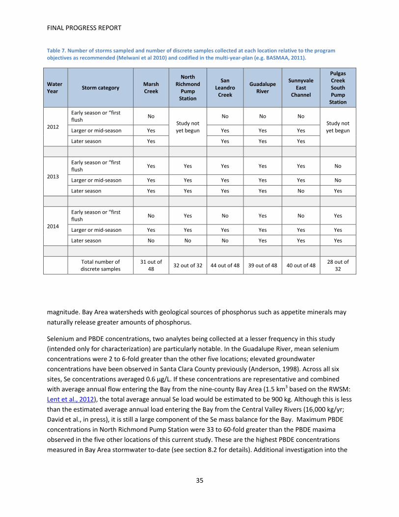
FINAL PROGRESS REPORT
35
Table 7. Number of storms sampled and number of discrete samples collected at each location relative to the program objectives as recommended (Melwani et al 2010) and codified in the multi-year-plan (e.g. BASMAA, 2011).
Water Year Storm category Marsh
Creek
North Richmond
Pump Station
San Leandro
Creek
Guadalupe River
Sunnyvale East
Channel
Pulgas Creek South Pump
Station
2012
Early season or “first flush No
Study not yet begun
No No No Study not yet begun Larger or mid-season Yes Yes Yes Yes
Later season Yes Yes Yes Yes
2013
Early season or “first flush Yes Yes Yes Yes Yes No
Larger or mid-season Yes Yes Yes Yes Yes No
Later season Yes Yes Yes Yes No Yes
2014
Early season or “first flush No Yes No Yes No Yes
Larger or mid-season Yes Yes Yes Yes Yes Yes
Later season No No No Yes Yes Yes
Total number of discrete samples
31 out of 48 32 out of 32 44 out of 48 39 out of 48 40 out of 48 28 out of
32
magnitude. Bay Area watersheds with geological sources of phosphorus such as appetite minerals may naturally release greater amounts of phosphorus.
Selenium and PBDE concentrations, two analytes being collected at a lesser frequency in this study (intended only for characterization) are particularly notable. In the Guadalupe River, mean selenium concentrations were 2 to 6-fold greater than the other five locations; elevated groundwater concentrations have been observed in Santa Clara County previously (Anderson, 1998). Across all six sites, Se concentrations averaged 0.6 µg/L. If these concentrations are representative and combined with average annual flow entering the Bay from the nine-county Bay Area (1.5 km3 based on the RWSM: Lent et al., 2012), the total average annual Se load would be estimated to be 900 kg. Although this is less than the estimated average annual load entering the Bay from the Central Valley Rivers (16,000 kg/yr; David et al., in press), it is still a large component of the Se mass balance for the Bay. Maximum PBDE concentrations in North Richmond Pump Station were 33 to 60-fold greater than the PBDE maxima observed in the five other locations of this current study. These are the highest PBDE concentrations measured in Bay Area stormwater to-date (see section 8.2 for details). Additional investigation into the

FINAL PROGRESS REPORT
36
Table 8. Synthesis of concentrations of pollutants of concern based on all quality assured data collected over the three sampling years at each location.
Analyzed but not now I had somedetected: Fenpropathrin, Esfenvalerate/Fenvalerate, Cyfluthrin, Allethrin, Prallethrin, Phenothrin, Resmethrin. All Hardness results in WY 2013 were censored.
Analyte Name Unit
Number(%
detect)Mean
(std.error)
Number(%
detect)Mean
(std.error)
Number(%
detect)Mean
(std.error)
Number(%
detect)Mean
(std.error)
Number(%
detect)Mean
(std.error)
Number(%
detect)Mean
(std.error)SSC mg/L 101 108 117 136 137 96 204 56.8 115 157 232 56.5
(94%) (97%) (95%) (100%) (98%) (99%) (23.5) (5.57) (13.8) (12.3) (31.4) (6.27)ΣPCB ng/L 22 32 44 39 40 29 1.25 13.8 8.01 14.3 104 505
(100%) (100%) (100%) (100%) (100%) (100%) (0.258) (1.57) (1.16) (2.4) (27.5) (261)Total Hg ng/L 31 32 44 39 40 31 38.4 39.6 106 212 47.6 18.2
(100%) (100%) (100%) (100%) (100%) (100%) (9.62) (7.8) (24.2) (35.9) (6.68) (2.39)Total MeHg ng/L 20 16 30 27 27 20 0.291 0.208 0.397 0.504 0.295 0.189
(90%) (100%) (100%) (100%) (93%) (100%) (0.0741) (0.0633) (0.0663) (0.0677) (0.0376) (0.033)TOC mg/L 30 32 44 40 40 28 7.13 11.2 8.24 12.2 10.1 20.5
(100%) (100%) (100%) (100%) (100%) (100%) (0.34) (1.82) (0.462) (1.96) (1.1) (5.54)NO3 mg/L 28 32 45 36 41 28 0.569 0.976 0.425 0.917 0.472 0.466
(96%) (100%) (100%) (100%) (100%) (100%) (0.0402) (0.143) (0.0659) (0.099) (0.0872) (0.0864)Total P mg/L 30 32 44 40 41 28 0.415 0.384 0.288 0.414 0.411 0.29
(100%) (100%) (100%) (100%) (100%) (100%) (0.0441) (0.0256) (0.024) (0.0376) (0.0429) (0.047)PO4 mg/L 30 31 45 40 41 28 0.0987 0.218 0.1 0.15 0.128 0.124
(100%) (100%) (100%) (100%) (100%) (100%) (0.0074) (0.0141) (0.00412) (0.0156) (0.00905) (0.0189)Hardness mg/L 4 5 8 7 8 6 176 129 56.5 138 124 69.8
(100%) (100%) (100%) (100%) (100%) (100%) (19.3) (38.6) (4.94) (12.7) (32.6) (12)Total Cu ug/L 8 8 11 10 10 7 13.7 22.5 16.2 21.6 17.9 43.9
(100%) (100%) (100%) (100%) (100%) (100%) (3.59) (4.49) (3.07) (2.87) (1.88) (10.1)Dissolved Cu ug/L 8 8 11 10 10 7 2.74 8.45 5.98 5 5.5 18.6
(100%) (100%) (100%) (100%) (100%) (100%) (0.588) (1.53) (0.682) (0.939) (1.09) (3.91)Total Se ug/L 8 8 11 10 10 7 0.742 0.409 0.223 1.31 0.606 0.292
(100%) (100%) (100%) (100%) (100%) (100%) (0.103) (0.0638) (0.019) (0.252) (0.147) (0.0632)Dissolved Se ug/L 8 8 11 10 10 7 0.647 0.366 0.166 1.07 0.519 0.244
(100%) (100%) (100%) (100%) (100%) (100%) (0.0886) (0.0586) (0.0149) (0.266) (0.146) (0.0526)Carbaryl ng/L 8 8 12 10 10 7 3.63 21.6 5.82 29.5 6.5 105
(25%) (88%) (50%) (90%) (40%) (100%) (2.39) (4.72) (2.11) (6.87) (2.78) (26.3)Fipronil ng/L 8 8 11 10 10 7 12.2 6.31 10.1 11.3 6.5 3.29
(100%) (75%) (91%) (100%) (90%) (86%) (1.19) (1.92) (1.89) (1.56) (1.13) (0.68)ΣPAH ng/L 4 4 5 11 6 6 140 527 1260 416 1350 1660
(100%) (100%) (100%) (100%) (100%) (100%) (46.5) (279) (494) (116) (455) (1070)ΣPBDE ng/L 4 5 5 5 6 6 27 789 28.5 60.8 47 45.6
(100%) (100%) (100%) (100%) (100%) (100%) (10.1) (644) (11.7) (18.3) (16) (13.1)Delta/ Tralomethrin ng/L 8 8 10 10 9 7 1.5 2.29 0.391 0.852 1.77 0.386
(75%) (75%) (40%) (50%) (89%) (43%) (0.637) (0.818) (0.207) (0.328) (0.469) (0.205)Cypermethrin ng/L 8 8 11 10 10 7 11.7 4.84 0.368 1.49 3.29 2.42
(88%) (100%) (55%) (70%) (80%) (100%) (8.24) (1.38) (0.115) (0.512) (0.63) (0.663)Cyhalothrin lambda ng/L 7 7 9 10 8 6 1.23 1.1 0.616 0.556 0.656 0.35
(86%) (100%) (56%) (70%) (75%) (83%) (0.486) (0.228) (0.376) (0.174) (0.296) (0.12)Permethrin ng/L 8 8 11 10 10 7 6.08 17.7 3.59 10.5 21.8 10.7
(75%) (100%) (55%) (80%) (100%) (86%) (2.29) (5.91) (1.24) (2.34) (3.61) (3.03)Bifenthrin ng/L 8 8 11 10 10 7 75.2 5.88 8.08 5.29 8.01 5.14
(100%) (100%) (91%) (90%) (90%) (100%) (29.9) (0.796) (2.69) (1.18) (1.95) (1.81)

FINAL PROGRESS REPORT
37
source-release processes of PBDE that are specific to Richmond, and lacking in the other watersheds, would be needed to better understand this result.
Concentration sampling during the three water years at the six locations has in part confirmed previously known or suspected high leverage watersheds (i.e. mercury in Guadalupe, PCBs in Sunnyvale East Channel and Pulgas Creek South). Concentration results have also raised some questions about certain pollutants in other watersheds (e.g. upper versus lower watershed Hg concentrations in San Leandro Creek, PBDE concentrations in North Richmond Pump Station). More sampling under a broader range of storm events (early season and first flush, larger storms during the mid-season and later season storms) would improve characterization of pollutants in those watersheds and increase confidence in the relative magnitude between watersheds and average annual loads estimates (baseline concentrations) that might form the basis for assessing trends (MQ3) at some future time. Although not the subject of this report, the RMP has provided funding to support the development of a POC loadings synthesis document (McKee et al. in preparation) and a trends strategy document (slated for preparation in summer 2015). A more thorough evaluation of existing data as a baseline for the trends management questions will be completed through those efforts.
5.5 Loads of pollutants of concern computed for each sampling location One of the primary goals of this project and a key management question of the Small Tributary Loading Strategy was to estimate the annual loads of POCs from tributaries to the Bay (MQ2). In particular, large loads of POCs entering sensitive Bay margins are likely to have a disproportionate impact on beneficial uses (Greenfield and Allen, 2013). As described in the climatic section (5.2), given that the relationship between climate (manifested as either rainfall or resulting discharge) and watershed loads follows a power function, estimates of long-term average loads for a given watershed are highly influenced by samples collected during wetter than average conditions and rare high magnitude storm events. Comparing loads estimates between the sites was confounded by relatively small sample datasets collected during climatically dry years. However, based on data collected, average annual loads estimates for each sampling location have now been computed. Accepting these caveats, the following observations are made on the total wet season loads estimates at the six locations.
The magnitude of the total loads between watersheds is largely driven by drainage area of each watershed. In terms of total wet season loads from each of the six watersheds, the largest watershed sampled is the Guadalupe River, which also has the largest load for every pollutant estimated in this study. Conversely, Pulgas Creek South Pump Station is the smallest watershed in the study and has the lowest total wet season load (except for PCBs). As another example, methylmercury in San Leandro Creek (8.9 km2) and Guadalupe River (236 km2) have similar concentrations but Guadalupe River discharges more than 10x the total mass of methylmercury given the much greater overall discharge of runoff volume and sediments. There is one significant exception. As mentioned, Pulgas Creek Pump Station South exports a disproportionately large PCB load, greater than Lower Marsh Creek (160x larger), North Richmond Pump Station (3.3x larger), San Leandro Creek (15x larger), and Sunnyvale Channel (WY 2013 only, 25x larger) (Table 9).

FINAL PROGRESS REPORT
38
Table 9. Loads of pollutants of concern during the sampling years at each sampling location.
Site Water Year
Discharge (Mm3) SS (t) TOC (kg) PCBs (g) HgT (g) MeHgT
(g) NO3 (kg) PO4 (kg)
Total P (kg)
Loads Confidence Loads Quality
Marsh Creeka
2012 1.61 233 11,380 1.34 64.0 0.262 956 175 578 Moderate
(PCBs) Low (Hg)
Lack of sample data during storms that cause runoff and
sediment transport through the upper watershed reservoir and
data during a wet year.
2013 5.82 2,703 39,500 16.0 408 2.78 3,474 666 4,212
2014 1.34 202 9,257 1.20 30.7 0.217 786 148 479
North Richmond
Pump Stationb
2012 - - - - - - - - -
Moderate Lack of data during wet year. 2013 0.795 35.7 6,353 8.14 16.0 0.200 761 161 215
2014 0.499 20.4 6,197 4.76 15.8 0.117 478 101 186
San Leandro Creekc
2012 7.30 158 40,483 16.4 221 1.57 1,973 571 1,404
Low
Lack of a robust discharge rating curve for higher flows; lack of
data during reservoir release and during a wet year.
2013 7.21 223 52,274 15.0 213 1.58 2,801 674 1,334
2014 0.243 28.0 1,840 1.93 25.4 2.89 97.1 23.4 70.6
Guadalupe River
2012 25.8 2,1061 154,379 123 2,039 6.13 20,879 2,498 6,023 High (PCBs)
Low (Hg)
Lack of long duration and high intensity storms sampled for Hg release from upper watershed.
Confidence in PCB data supported by previous studies.
2013 35.5 4,4641 238,208 309 5,476 13.6 25,775 3,771 10,829
2014 16.75 1,094 106,141 97.2 1,519 4.29 13,182 1,723 4,172
Sunnyvale East
Channeld
2012 1.31 56.4 8,227 50.9 25.9 0.382 335 139 395
Moderate
Lack of data during wet year. High variability in PCB
concentrations between storm events.
2013 1.51 508 8,685 87.9 87.6 3.26 369 159 689
2014 1.01 89.0 12,040 74.4 27.9 0.669 336 135 343
Pulgas Creek Pump
Statione
2012 - - - - - - - - -
Low
A lower quality (FWMC) approach applied to loads
calculations. Lack of data during a wet year. High variability in PCB concentrations between
storm events.
2013 0.165 10.9 1,539 21.8 3.07 0.0291 41.1 12.8 33.0
2014 0.08 5.31 764 11.8 1.48 0.0141 20.1 6.31 16.1 a Marsh Creek wet season loads are reported for the period of record 12/01/11 – 4/26/12, 10/19/12 – 4/18/13 and 11/06/13 – 4/30/14. b North Richmond Pump Station wet season loads are reported for the period of record 11/01/12 – 4/30/13 and 10/16/13 – 4/30/14. c San Leandro Creek wet season loads are reported for the period of record 12/01/11 – 4/30/12, 11/01/12 – 4/18/13 and 11/01/13 – 4/30/14. d Sunnyvale East Channel wet season loads are reported for the period of record 12/01/11 – 4/30/12, 10/01/12 – 4/30/13 and 10/01/13 – 4/30/14. e Pulgas Creek South Pump Station loads are estimates provided for the entire wet seasons (10/01/12 – 4/30/13 and 10/01/13 – 4/30/14) however monitoring only occurred during the period 12/17/2012 – 3/15/2012 and 10/22/13 – 4/30/14. Monthly loads for the non-monitored period were extrapolated using regression equations developed for the monthly rainfall and corresponding monthly (or partial month) contaminant load.

FINAL PROGRESS REPORT
39
Comparison of total wet season loads between water years at the sites highlighted show how loads estimates can be highly variable even during three drier than average years. Additionally, the size and intensity of the storm events in the different regions where the sampling sites were located greatly impacted the load variation from year-to-year and between sampling locations. For example, PCB loads in Guadalupe River and San Leandro Creek were approximately 3- and 7-fold greater in WY 2012 than in WY 2014, whereas loads of PCBs were 13- and 8-fold larger in WY 2013 relative to WY2012 in Lower Marsh Creek and Sunnyvale East Channel, where the late November and December 2012 (WY2013) storms were comparatively larger events. Even when normalized to total discharge (in other words, the flow-weighted mean concentration [FWMC]), Sunnyvale East Channel transported 7-fold as much sediment in WY 2013 than WY 2012, whereas the FWMC of suspended sediment in San Leandro Creek was the same in WYs 2012 and 2013 and 5-fold greater in WY 2014 despite much lower flow. The relationship between FWMC and discharge (either at the annual or individual flood scale) can be used as an indicator of when enough data have been collected to characterize the site adequately to answer our management questions. FWMC should continue to increase relative to storm magnitude until watershed sources are exhausted; locations and analytes that reach that maximum will have sufficient data to compute reliable long term average annual loads. With the data currently in hand, attempts to estimate average annual loads will be biased low.
In light of these climatic considerations as well as the known data quality considerations and challenges at each of the sampling locations, the two far-right columns in Table 9 note the remaining level of confidence in the annual loads estimates as well as the main issues at each site which warrant the confidence level rating. Any future sampling at each of these locations should seek to alleviate these issues and to raise the quality of the data in relation to answering management questions.
5.6. Comparison of regression slopes and normalized loads estimates between watersheds
One of our key activities in relation to the Small Tributary Loading Strategy is improving our understanding of which Bay tributaries (including stormwater conveyances) contribute most to Bay impairment from pollutants of concern (MQ1) and therefore potentially represent watersheds where management actions should be implemented to have the greatest beneficial impact (MQ4). Multiple factors influence the treatability of pollutant loads in relation to impacts to San Francisco Bay. Conceptually, a large load of pollutant transported on a relatively small mass of sediment is more treatable than less polluted sediment. Therefore, the graphical function between either sediment concentration or turbidity provides a first order mechanism for ranking relative treatability of watersheds (Figure 2A). This method is valid for pollutants that are dominantly transported in a particulate form (total mercury and the sum of PCBs are good examples but pyrethroid pesticides and PBDEs may also be considered in this group) and when there is relatively little variation in the particle ratios between water years or storms or at least less variation than seen between watersheds. Note data presented at the October 2013 SPLWG meeting demonstrated that this assumption is sometimes violated and influences our perception of relative ranking.
These issues accepted, based on the ratios between turbidity and Hg, runoff derived from less urbanized upper portions of San Leandro Creek watershed and runoff from the Guadalupe River watershed exhibit

FINAL PROGRESS REPORT
40
the greatest particle ratios for total mercury (Figure 2). Sunnyvale East Channel, Marsh Creek and Pulgas Creek South Pump Station appear to have relatively low particle ratios for total mercury, although, Marsh Creek has not been observed under wet conditions when the possibility of mercury release from historic mining sources exists. The relative nature of these rankings has not changed in relation to the previous reports (McKee et al., 2013; Gilbreath et al., 2014).
In contrast, for the sum of PCBs, Pulgas Creek South Pump Station and Sunnyvale East Channel exhibit the highest particle ratios among these six watersheds, with urban sourced runoff from Guadalupe River and North Richmond Pump Station ranked 3rd and 4th as indicated by the turbidity-PCB graphical relation (Figure 2). Marsh Creek exhibits very low particle ratios for PCBs, an observation that is unlikely to change with additional samples given the likelihood of relatively low pollutant sources and relatively low variability of release-transport processes. Unlike for Hg, new data collected during WYs 2013 and 2014 alters the relative PCB rankings based on this graphical analysis providing an example of the influence of either low sample numbers or the random nature of sample capture on the resulting interpretation of particle ratios (as discussed in the October 2013 SPLWG meeting). Given the relatively wide confidence intervals around these lines (not shown) and the collection during relatively dry years, the relative nature of these regression equations may change if there are any future samples completed.
Figure 2. Comparison of regression slopes between watersheds based on data collected during sampling for A) Total Mercury and B) PCBs. Turbidity range shown on graphs represents minimum and maximum turbidities for entire sampling period
A
B

FINAL PROGRESS REPORT
41
Another influence on potential treatability is the size of the watershed. Conceptually, a large load that is transported from a relatively small watershed and therefore in association with a relatively small volume of water is more manageable. Efforts to manage flows from the North Richmond Pump Station watershed exemplify this type of opportunity. Thus, area normalized loads (yields) provide another useful mechanism for first order ranking of watersheds (Table 10) in relation to ease of management. This method is more highly subject to climatic variation than the turbidity function/particle ratio method for ranking and therefore was done on climatically averaged loads. Despite these challenges, in a general sense, the relative rankings for PCBs exhibit a similar ranking to the particle ratio method; Pulgas Creek South Pump Station watershed ranked highest and Marsh Creek watershed ranked lowest. However the relative ranking of the other watersheds is not similar. In the case of mercury, Guadalupe River and San Leandro Creek exhibit the highest currently estimated yields corroborating the evidence from the particle ratio method. Similar to PCBs, the relative ranking of the other four watersheds is not similar to the particle ratio method. Given all our observations were during relatively dry years, it is difficult to know the certainty of the relative nature of the area-normalized estimates. For example, the relative rankings for suspended sediment loads normalized by unit area would likely change substantially with the addition of data from a water year that exceeds the climatic normal for each watershed; total phosphorus unit loads would also respond in a similar manner. For pollutants such as PCBs and total Hg that are found in specific source areas such as industrial and mining areas (Hg only) of these watersheds, release processes will likely be influenced by both climatic factors and sediment transport off impervious surfaces; also factors that are not likely well captured by the sampling that has occurred under relatively dry conditions.
6. Conclusions and next steps
6.1. Current and future uses of the data The monitoring program implemented during the study was designed primarily to improve estimates of watershed-specific and regional loads to the Bay (MQ2) and secondly, to provide baseline data to support evaluation of trends towards concentration or loads reductions in the future (conceptually one or two decades hence) (MQ3) (see introduction section) in compliance with MRP provision C.8.e. (SFRWRCB, 2009). Multiple metrics have been developed and presented in this report to support these management questions:
• Pollutant loads: Pollutant loading estimates can help measure relative delivery of pollutants to sensitive Bay margin habitats and support calibration and verification of the Regional Watershed Spreadsheet Model and resulting regional scale loading estimates.
• Flow Weighted Mean Concentrations: FWMC can help to identify when sufficient data has been collected to adequately characterize watershed processes in relation to a specific pollutant in the context of management questions.
• Sediment-pollutant particle ratios: Particle ratios can help identify relative watershed pollution levels on a particle basis and relates to treatment potential.
• Pollutant area yields: Pollutant yields can help identify pollutant sources and relates to treatment potential.

FINAL PROGRESS REPORT
42
Table 10. Climatically averaged area normalized loads (yields) ranked in relation to PCBs based on free flowing areas downstream from reservoirs (See Table 1 for areas used in the computations).
Unit
runoff (m)
SS (t/km2)
TOC (mg/m2)
PCBs (µg/m2)
HgT (µg/m2)
MeHgT (µg/m2)
NO3 (mg/m2)
PO4 (mg/m2)
Total P (mg/m2)
Marsh Creek 0.13 80.0 916 0.474 13.8 0.0423 79.7 15.1 76.6
North Richmond Pump Station 0.52 26.1 4,684 5.84 13.7 0.143 497 105 157
San Leandro Creek 0.95 53.3 5,957 3.36 55.4 0.260 317 81.9 216
Guadalupe River 0.24 272 1,926 20.3 282 0.196 169 28.1 116
Sunnyvale East Channel 0.17 33.6 1,220 9.44 5.95 0.116 45.8 19.3 63.9
Pulgas Creek Pump Station 0.63 41.8 5,907 84.6 11.8 0.111 158 49.2 127
• Correlation of pollutants: Finding co-related pollutants helps identify those watersheds with multiple sources and provides additional cost/benefit for management actions.
As discussed briefly in the introduction (section 1), as management effort focuses more and more on locating high leverage watersheds and patches within watersheds, the monitoring (and modeling) design is evolving.
6.2. What data gaps remain at current loads stations? With regard to addressing the main management endpoints (single watershed and regional watershed loads and baseline data for trends) that influenced the monitoring design recommended by Melwani et al 2010 and described in each iteration of the MYP (BASMAA, 2011; BASMAA, 2012; BASMAA, 2013), an important question that managers are asking is how to determine when sufficient data have been collected. Several sub-questions are important when trying to make this determination. Are the data representative of climatic variability; have storms and years been sampled well enough relative to expected climatic variation? Are the data representative of the source-release-transport processes of the pollutant of interest? In reality, these factors tend to juxtapose and after three years of monitoring during relatively dry climatic conditions, some data gaps remain for each of the monitoring locations.
• Marsh Creek watershed has been sampled for three WYs. Continuous turbidity data were rated excellent at Lower Marsh Creek. Ample lower watershed stormwater runoff data are now available at Lower Marsh Creek, but this site is lacking information on high intensity upper watershed rain events where sediment mobilization from the historic mercury mining area could occur. Any future sampling would ideally be focused on Hg and for storms of greater intensity preferably when spillage is occurring from the upstream reservoir. No further PCB data are recommended. The sampling design to achieve these goals could be revisited with the objective of increased cost efficiency for data gathering to support remaining unanswered management questions.

FINAL PROGRESS REPORT
43
• North Richmond Pump Station watershed has been sampled for two WYs (although data exist from a previous study [Hunt et al., 2012]). Additional data in relation to early season (seasonal 1st flush or early season storms) would help improve estimates of loads that could be averted from diversion of early season storms to wastewater treatment. Further data collection in relation to high concentrations of PBDEs would increase our understanding of PBDE source(s) in this watershed.
• San Leandro Creek watershed has been sampled for three WYs. San Leandro Creek received poor ratings on the quality of discharge information and completeness of turbidity data. The largest weakness is the scarcity of velocity measurements to adequately describe the stage-discharge rating curve for stages >2 feet and generate a continuous flow record. Additional velocity measurements are necessary to increase the accuracy and precision of discharge data for the site and support the computation of loads. There is currently no information on pollutant concentrations during reservoir releases, yet volumetrically, reservoir releases during WYs 2012 and 2013 were proportionally large but may have been atypical. Sample collection during release would help elucidate pollutant load contributions from the reservoir. Data collection during more intense rainstorms are also desirable for this site given the complex sources of PCBs and mercury in the watershed and the existence of areas of less intense land use and open space lending to likely relatively high inter-annual variability of water and sediment production.
• Guadalupe River watershed has been sampled at the Hwy 101 location during nine water years (WY 2003-2006, 2010-2014) to-date, but data are still lacking to adequately describe high intensity upper watershed rain events when mercury may still be released from sources in relation to historic mining activities. This type of information could help estimate the upper range of mercury loads from the mercury mining district and continue to help focus management attention. Further data collection in Guadalupe River watershed should focus on Hg sampling during high intensity storms. Further sampling of relatively frequent smaller runoff events is unnecessary and transport processes for PCBs are well supported by currently available data. The current sampling design is not cost-effective for gathering improved information to support management decisions in this watershed.
• Sunnyvale East Channel initially received poor quality data ratings for turbidity but this improved substantially in WYs 2013 and 2014. However, more storm event POC data are needed for establishing higher confidence in particle ratios, pollutant loads, FWMCs, and yields. A PCB source was apparently mobilized during the February 28, 2014 storm which had very high PCB concentrations, and this source seemed to continue to flush through the system in subsequent events. Because of this, our PCB regression with turbidity is not strong, creating uncertainty around the accuracy of the total PCB load estimate (e.g. what PCB sources might have moved through the system when we were not sampling?). Further data are needed in this watershed to better understand source-release-transport processes for PCBs.
• Based on the current review of the data, Pulgas Creek South Pump Station received a poor data quality rating for turbidity. Monitoring at this site was complicated by the logistical limitations of monitoring in a highly dynamic storm drain system. The challenging logistics of this site led to delays in the initiation of monitoring in WY 2013 as BASMAA/KLI worked to establish a

FINAL PROGRESS REPORT
44
monitoring plan and functional instrumentation configuration (e.g., during WY 2013, turbidity data were only collected during three of the seven wet season months due to these challenges). In addition, because this site was located within a storm drain and vault adjacent to a pump station, the periodic operation of the pumps likely contributed to turbidity spikes and generally noisy nature of the data. Following review of WY 2014 observations, it was decided to reject the whole turbidity data set from this site. Although not feasible under the scope of this project, BASMAA has suggested they may undertake further review of this dataset, including application of smoothing functions to better fit the pollutant data to the turbidity record and potentially improve the usability of these data. KLI collected a robust manual turbidity sample set in combination with the pollutant sampling. Although they did not accurately record the times of this sample collection and therefore a relationship between manual turbidity and the sensor turbidity record for discrete times cannot be developed, a relationship between manual collection and smoothed sensor data (e.g. smoothed over 15-30 minutes) could potentially be developed. This could then validate the data quality of the smoothed turbidity data, and allow future use of these data for the development of the turbidity-pollutant regressions. However, because of the dynamic nature of this system (e.g. the sensor record showed changes >500 NTU in a 15 minute period), the likelihood of forming acceptable regressions between pollutant data and smoothed turbidity data seems low. More importantly, the cyclical spiking of the turbidity record suggests resuspension of settled sediments during pump outs. If the turbidity sensor was measuring resuspension of sediment in the vault, the turbidity sensor was measuring the turbidity caused by that sediment when it initially entered the vault, as well as when it was resuspended; in other words, the sensor record includes in some portions twice-measured sediment/turbidity. Therefore, the continuous turbidity record likely does not accurately represent the turbidity within the system, and consequently an accurate, continuous record for any pollutant likely cannot be established using the turbidity surrogate regression method even in the event that a pollutant-turbidity regression could be developed through smoothing. The sampling program began at this location (and North Richmond Pump Station) in WY 2013 as compared to WY 2012 at the other sites, and so despite being one of the most logistically challenging sites to set up for monitoring, BASMAA/KLI also had the least amount of time to execute it (arguably North Richmond Pump Station was also logistically challenging but SFEI had already completed two years of sampling at this location for another project, during which some of the instrumentation set-up challenges had been worked through). Due to both the delay in monitoring initiation at Pulgas combined with the very low rainfall in WY 2013, only a single storm was monitored and therefore very little data was available from WY 2013 in which to assess these issues. In short, although this has been a three-year project, this is really the first year that a substantial dataset has been available to evaluate for the Pulgas Ck Pump Station site. On the positive side, there are nearly two full wet seasons of flow data as well as seven storms worth of pollutant data, including the highest PCB concentrations observed to-date in the Bay Area. Despite challenges with the continuous turbidity record, these other data are valuable and less robust estimates of load are possible based on the FWMC approach. Additionally, because KLI also collected manual turbidity samples during pollutant sample collection, the pollutant data could potentially still be used to estimate loads using turbidity

FINAL PROGRESS REPORT
45
surrogate regression if a high quality relationship between the manually collected turbidity record and a continuous record could be established. Now that the monitoring challenges for this site are better understood, additional effort to improve the continuous turbidity monitoring at this location would be desirable to increase confidence in particle ratios, pollutant loads, FWMCs, and yields.
6.3. Next Steps Recent discussions between BASMAA and the Region 2 Regional Water Quality Control Board in relation to reissuing the MRP (and discussion at the October 2013 and May 2014 SPLWG meetings) have highlighted the increasing focus towards finding watersheds and land areas within watersheds for management focus (MQ4). The monitoring design described in this report is not appropriate for this increasing management focus. There are various alternative monitoring designs that are more cost-effective for addressing the increasing focus in the second MRP permit term towards finding watersheds and land areas within watersheds for management attention while still supporting the other STLS management questions in a programmatic manner. The challenge for the STLS and SPWLG is finding the right balance between the different alternatives within budget constraints. Sampling during WY 2015 is using the following reconnaissance characterization design:
• Collaboration with stormwater Countywide programs to identify locations with possible PCB and/or mercury sources (based on a GIS based analysis)
• Focused sampling in older industrial drainages (some of which are tidally influenced) • Composite sampling: 1 composite per storm/per analyte for PCB, total mercury, total metals,
SSC, grain size, TOC/DOC; 5-15 aliquots per composite sample • Pilot testing passive sediment samplers
The advantage of the reconnaissance sampling design is flexibility and given recent advances on the development of the RWSM (SFEI in preparation) have indicated the value of the data collected previously using the reconnaissance design (McKee et al., 2012), it seems likely that the reconnaissance design may end up being the most cost-effective going forward over the next three or more years. Data and information gathered over the last 10+ years guided by the SPLWG and STLS will continue to help guide the development of a cost effective monitoring design to adapt to changing management needs.

FINAL PROGRESS REPORT
46
7. References Amweg, E., D.P. Weston and N.M. Ureda. Use and toxicity of pyrethroid pesticides in the central valley,
California, USA. Environmental Toxicology and Chemistry. vol. 24, no. 4, pp. 966–972.
Anderson B., Hunt, J., Markiewicz, D., Larsen, K. 2010. Toxicity in California Waters. Surface Water Ambient Monitoring Program. California State Water Resources Control Board. Sacramento, CA.
Anderson, D.W., 1998. Natural levels of nickel, selenium, and arsenic in the South San Francisco Bay area. Report prepared for the City of San Jose, Environmental Services Department by the Institute for Research in Environmental Engineering and Science, San Jose, Ca. 15pp.
Balogh, S. J., Y. Huang, H. J. Offerman, M. L. Meyer, and D. K. Johnson. 2002. Episodes of Elevated Methylmercury Concentrations in Prairie Streams. Environmental Science and Technology 36:1665 -1670.
Barringer, J. L., M. L. Riskin, Z. Szabo, P. A. Reilly, R. Rosman, J. L. Bonin, J. M. Fischer, and H. A. Heckathorn. 2010. Mercury and Methylmercury Dynamics in a Coastal Plain Watershed, New Jersey, USA. Water Air and Soil Pollution 212:251-273.
Bartley, R., W. J. Speirs, T. W. Ellis, and D. K. Waters. 2012. A review of sediment and nutrient concentration data from Australia for use in catchment water quality models. Marine Pollution Bulletin 65:101-116.
BASMAA, 2011. Small Tributaries Loading Strategy Multi-Year Plan (MYP) Version 2011. A document developed collaboratively by the Small Tributaries Loading Strategy Work Group of the Regional Monitoring Program for Water Quality in the San Francisco Estuary (RMP): Lester McKee, Alicia Gilbreath, Ben Greenfield, Jennifer Hunt, Michelle Lent, Aroon Melwani (SFEI), Arleen Feng (ACCWP) and Chris Sommers (EOA/SCVURPPP) for BASMAA, and Richard Looker and Tom Mumley (SFRWQCB). Submitted to the Water Board, September 2011, in support of compliance with the Municipal Regional Stormwater Permit, provision C.8.e. http://www.swrcb.ca.gov/rwqcb2/water_issues/programs/stormwater/MRP/2011_AR/BASMAA/B2_2010-11_MRP_AR.pdf
BASMAA, 2012. Small Tributaries Loading Strategy Multi-Year Plan (MYP) Version 2012A. A document developed collaboratively by the Small Tributaries Loading Strategy Work Group of the Regional Monitoring Program for Water Quality in the San Francisco Estuary (RMP): Lester McKee, Alicia Gilbreath, Ben Greenfield, Jennifer Hunt, Michelle Lent, Aroon Melwani (SFEI), Arleen Feng (ACCWP) and Chris Sommers (EOA/SCVURPPP) for BASMAA, and Richard Looker and Tom Mumley (SFRWQCB). Submitted to the Water Board, September 2011, in support of compliance with the Municipal Regional Stormwater Permit, provision C.8.e. http://www.waterboards.ca.gov/sanfranciscobay/water_issues/programs/stormwater/MRP/2012_AR/BASMAA/BASMAA_2011-12_MRP_AR_POC_APPENDIX_B4.pdf
FINAL PROGRESS REPORT
47
Birgand, F., C. Faucheux, G. Gruau, B. Augeard, F. Moatar, and P. Bordenave. 2010. Uncertainties in assessing annual ntirate loads and concentration indicators: Part 1. Impact of sampling frequency and load estimation algorithms. Transactions of the Asabe 53:437-446.
Bradford, G. R., A. C. Chang, A. L. Page, D. Balhtar, J. A. Frampton, and H. Wright. 1996. Background Concentrations of Trace and Major Elements in California Soils Kearney Foundation of Soil Science.
Bradley, P. M., D. A. Burns, K. Riva-Murray, M. E. Brigham, D. T. Button, L. C. Chasar, M. Marvin-DiPasquale, M. A. Lowery, and C. A. Journey. 2011. Spatial and Seasonal Variability of Dissolved Methylmercury in Two Stream Basins in the Eastern United States. Environmental Science & Technology 45:2048-2055.
Chalmers, A. T., D. P. Krabbenhoft, P. C. Van Metre, and M. A. Nilles. 2014. Effects of urbanization on mercury deposition and accumulation in New England. Environmental Pollution 192:104-112.
Chow, V. T. 1959. Open-Channel Hydraulics. McGraw-Hill, Inc. 680pp.
Conaway, C. H., E. B. Watson, J. R. Flanders, and A. R. Flegal. 2003. Mercury deposition in a tidal marsh of south San Francisco Bay downstream of the historic New Almaden mining district, California. Marine Chemistry 90:175-184.
David, N., Gluchowski, D.C, Leatherbarrow, J.E, Yee, D., and McKee, L.J, (in press). Evaluation of loads of mercury, selenium, PCBs, PAHs, PBDEs, dioxins, and organochlorine pesticides from the Sacramento-San Joaquin River Delta to San Francisco Bay. Water Environment Research, 87, xx-xx.
Davis, J.A., Hetzel, F., Oram, J.J., and McKee, L.J., 2007. Polychlorinated biphenyls (PCBs) in San Francisco Bay. Environmental Research 105, 67-86. http://www.sciencedirect.com/science/article/pii/S0013935107000400
Davis, J.A., Yee, D., Grenier, L., McKee, L.J., Greenfield, B.A., Looker, R., Austin, C., Marvin-DePasquale, M., Brodberg, R., and Blum, J., 2012. Reducing methylmercury accumulation in the food webs of San Francisco Bay and its local watersheds. Environmental Research 119, 3-26. http://www.sciencedirect.com/science/article/pii/S001393511200285
Dillon, P. J., and Kirchner, W.B. 1975. The effects of geology and land use on the export of phosphorus from watersheds. Water Research 9:135-148.
Domagalski, J. 2001. Mercury and methylmercury in water and sediment of the Sacramento River Basin, California. Applied Geochemistry 16:1677.
Eckley, C. S. and B. Branfireun. 2008. Mercury mobilization in urban stormwater runoff. Science of the Total Environment 403:164-177.
Ensminger, M.P., Budd, R., Kelley, K.C., and Goh, K.S., 2012. Pesticide occurrence and aquatic benchmark exceedances in urban surface waters and sediments in three urban areas of California, USA, 2008-
FINAL PROGRESS REPORT
48
2011. Environmental Monitoring and Assessment http://www.springerlink.com/content/g11r274187122410/
Fitzgerald, W. F., D. R. Engstrom, R. P. Mason, and E. A. Nater. 1998. The case for atmospheric mercury contamination in remote areas. Environmental Science and Technology 32:1-7.
Foster GD, Lippa KA, Miller CV. Seasonal concentrations of organic contaminants at the fall line of the Susquehanna River Basin and estimated fluxes to Northern Chesapeake Bay, USA. Environ Toxicol Chem 2000a; 19(4):992-1001.
Foster GD, Roberts EC Jr., Gruessner B, Velinsky DJ. Hydrogeochemistry and transport of organic contaminants in an urban watershed of Chesapeake Bay USA. App Geochem 2000b; 15:901-15.
Gilbreath, A.N., Gluchowski, D.C., Wu, J., Hunt, J.A., and McKee, L.J., 2014. Pollutants of concern (POC) loads monitoring data progress report, water year (WYs) 2012 and 2013. A technical report prepared for the Regional Monitoring Program for Water Quality in San Francisco Bay (RMP), Sources, Pathways and Loadings Workgroup (SPLWG), Small Tributaries Loading Strategy (STLS). Contribution No. 708. San Francisco Estuary Institute, Richmond, California. http://www.sfei.org/sites/default/files/Final_WY%202013_POC%20loads%20progress%20report_24%20February%202014_web%20posted.pdf
Gilbreath, A., Yee, D., McKee, L.J., 2012. Concentrations and loads of trace contaminants in a small urban tributary, San Francisco Bay, California. A Technical Report of the Sources Pathways and Loading Work Group of the Regional Monitoring Program for Water Quality: Contribution No. 650. San Francisco Estuary Institute, Richmond, California. 40pp. http://www.sfei.org/sites/default/files/Z4LA_Final_2012May15.pdf
Gomez-Gutierrez, A. I., E. Jover, L. Bodineau, J. Albaiges, and J. M. Bayona. 2006. Organic contaminant loads into the Western Mediterranean Sea: Estimate of Ebro River inputs. Chemosphere 65:224-236.
Greenfield, B.K., and Allen, R.M., 2013. Polychlorinated biphenyl spatial patterns in San Francisco Bay forage fish. Chemosphere 90, 1693–1703.
Guan YF, Wang J, Ni HG, Luo XJ, Mai BX, Zeng EY., 2007. Riverine inputs of polybrominated diphenyl ethers from the Pearl River Delta (China) to the coastal ocean. Environ Sci Tech 41(17):6007-13.
Henjum, M. B., R. M. Hozalski, C. R. Wennen, W. A. Arnold, and P. J. Novak. 2010. Correlations between in situ sensor measurements and trace organic pollutants in urban streams. Journal of Environmental Monitoring 12:225-233.
Howell NL, Lakshmanan D, Rifai HS, Koenig L. PCB dry and wet weather concentration and load comparisons in Houston-area urban channels. Sci Tot Environ 2011; 409: 1867-1888.
Hudak, P. F. and K. E. Banks. 2006. Compositions of first flush and composite storm water runoff in small urban and rural watersheds, north-central Texas. Urban Water Journal 3:43-49.

FINAL PROGRESS REPORT
49
Hunt, J., Gluchowski, D., Gilbreath, A., and McKee, L.J., 2012. Pollutant Monitoring in the North Richmond Pump Station: A Pilot Study for Potential Dry Flow and Seasonal First Flush Diversion for Wastewater Treatment. A report for the Contra Costa County Watershed Program. Funded by a grant from the US Environmental Protection Agency, administered by the San Francisco Estuary Project. San Francisco Estuary Institute, Richmond, CA. http://www.sfei.org/sites/default/files/NorthRichmondPumpStation_Final_19112012_ToCCCWP.pdf
Hurley, J. P., J. M. Benoit, C. L. Babiarz, M. M. Shafer, A. W. Andren, J. R. Sullivan, R. Hammond, and D. A. Webb. 1995. Influences of watershed characteristics on mercury levels in Wisconsin rivers. Environmental Science and Technology 29:1867-1875.
Hwang, H.-M. and G. D. Foster. 2008. Polychlorinated biphenyls in stormwater runoff entering the tidal Anacostia River, Washington, DC, through small urban catchments and combined sewer outfalls. Journal of Environmental Science and Health Part a-Toxic/Hazardous Substances & Environmental Engineering 43:567-575.
Inman, D. L. and S. A. Jenkins. 1999. Climate change and the episodicity of sediment flux of small California River. The Journal of Geology 107:251-270.
Keppeler, E. T. 2012. Sediment production in a coastal watershed: legacy, land use, recovery, and rehabilitation. Pages 69-77 in R. B. Standiford, T. J. Weller, D. D. Piirto, and J. D. Stuart, editors. Proceedings of coast redwood forests in a changing California: A symposium for scientists and managers, Albany, CA.
Kocman, D., M. Horvat, N. Pirrone, and S. Cinnirella. 2013. Contribution of contaminated sites to the global mercury budget. Environmental Research 125:160-170.
Kronvang, B. and A. J. Bruhn. 1996. Choice of sampling strategy and estimation method for calculating nitrogen and phosphorus transport in small lowland streams. Hydrological Processes 10:1483-1501.
Lamborg, C. H., W. F. Fitzgerald, A. W. H. Damman, J. M. Benoit, P. H. Balcom, and D. R. Engstrom. 2002. Modern and historic atmospheric mercury fluxes in both hemispheres: Global and regional mercury cycling implications. Global Biogeochemical Cycles 16:1104.
Lawson, N. M., R. P. Mason, and J.-M. Laporte. 2001. The fate and transport of mercury, methylmercury, and other trace metals in chesapeake bay tributaries. Water Research 35:501.
LeBlanc, L. A. and K. M. Kuivila. 2008. Occurrence, distribution and transport of pesticides into the Salton Sea Basin, California, 2001-2002. Hydrobiologia 604:151-172.
Lent, M.A. and McKee, L.J., 2011. Development of regional suspended sediment and pollutant load estimates for San Francisco Bay Area tributaries using the regional watershed spreadsheet model (RWSM): Year 1 progress report. A technical report for the Regional Monitoring Program for Water Quality, Small Tributaries Loading Strategy (STLS). Contribution No. 666. San Francisco Estuary

FINAL PROGRESS REPORT
50
Institute, Richmond, CA. http://www.sfei.org/sites/default/files/RWSM_EMC_Year1_report_FINAL.pdf
Lent, M.A., Gilbreath, A.N., and McKee, L.J., 2012. Development of regional suspended sediment and pollutant load estimates for San Francisco Bay Area tributaries using the regional watershed spreadsheet model (RWSM): Year 2 progress report. A technical progress report prepared for the Regional Monitoring Program for Water Quality in San Francisco Bay (RMP), Small Tributaries Loading Strategy (STLS). Contribution No. 667. San Francisco Estuary Institute, Richmond, California. http://www.sfei.org/sites/default/files/RWSM_EMC_Year2_report_FINAL.pdf
Lewicki, M., and McKee, L.J, 2009. Watershed specific and regional scale suspended sediment loads for Bay Area small tributaries. A technical report for the Sources Pathways and Loading Workgroup of the Regional Monitoring Program for Water Quality: SFEI Contribution #566. San Francisco Estuary Institute, Oakland, CA. 28 pp + Appendices. http://www.sfei.org/sites/default/files/566_RMP_RegionalSedimentLoads_final_web.pdf
Lewis, J. 1996. Turbidity-controlled suspended sediment sampling for runoff-event load estimation. Water Resources Research 32:2299-2310.
Lin, Y., R. Vogt, and T. Larssen. 2012. Environmental mercury in China: A review. Environmental Toxicology and Chemistry 31:2431-2444.
Line, D. E. 2013. Effect of development on water quality for seven streams in North Carolina. Environmental Monitoring and Assessment 185:6277-6289.
Ma, J.-S., J.-H. Kang, M. Kayhanian, and M. K. Stenstrom. 2009. Sampling Issues in Urban Runoff Monitoring Programs: Composite versus Grab. Journal of Environmental Engineering.
Marsalek, J. and H. Y. F. Ng. 1989. Evaluation of pollution loadings from urban nonpoint sources: methodology and applications. Journal Of Great Lakes Research 15:444-451.
Mason RP, Sullivan KA. Mercury and methylmercury transport through an urban watershed. Water Research 1998:32:321-30.
McKee, L.J., Gilbreath, A.N., Hunt, J.A., Wu, J., and Yee, D., (in preparation). Sources, Pathways and Loadings: Multi-Year Synthesis. A technical report prepared for the Regional Monitoring Program for Water Quality in San Francisco Bay (RMP), Sources, Pathways and Loadings Workgroup (SPLWG), Small Tributaries Loading Strategy (STLS). Contribution No. xxx. San Francisco Estuary Institute, Richmond, California.
McKee, L.J., Gilbreath, A.N., Wu, J., Kunze, M.S., Hunt, J.A., 2014. Estimating Regional Pollutant Loads for San Francisco Bay Area Tributaries using the Regional Watershed Spreadsheet Model (RWSM): Year’s 3 and 4 Progress Report. A technical report prepared for the Regional Monitoring Program for Water Quality in San Francisco Bay (RMP), Sources, Pathways and Loadings Workgroup (SPLWG), Small Tributaries Loading Strategy (STLS). Contribution No. 737. San Francisco Estuary Institute,

FINAL PROGRESS REPORT
51
Richmond, California. http://www.sfei.org/sites/default/files/737%20RWSM%20Progress%20Report%20Y3_4%20for%20the%20WEB.pdf
McKee, L.J., Gilbreath, A.N., Gluchowski, D.C., Hunt, J.A., and Yee, D., 2013. Quality assurance methods for continuous rainfall, run-off, and turbidity data. A draft report prepared for Bay Area Stormwater Management Agencies Association (BASMAA), and the Regional Monitoring Program for Water Quality in San Francisco Bay (RMP) Sources Pathways and Loadings Workgroup (SPLWG),Small Tributaries Loading Strategy (STLS). Contribution No. xxx. San Francisco Estuary Institute, Richmond, CA. http://www.sfei.org/sites/default/files/739.pdf
McKee, L.J., Gluchowski, D.C., Gilbreath, A.N., and Hunt, J.A., 2013. Pollutants of concern (POC) loads monitoring data progress report, water year (WY) 2012. A technical report prepared for the Regional Monitoring Program for Water Quality in San Francisco Bay (RMP), Sources, Pathways and Loadings Workgroup (SPLWG), Small Tributaries Loading Strategy (STLS). Contribution No. 690. San Francisco Estuary Institute, Richmond, California. See pages 574-633 of the report link below: http://www.swrcb.ca.gov/rwqcb2/water_issues/programs/stormwater/UC_Monitoring_Report_2012.pdf
McKee, L.J., Gilbreath, A.N., Hunt, J.A., and Greenfield, B.K., 2012. Pollutants of concern (POC) loads monitoring data, Water Year (WY) 2011. A technical report prepared for the Regional Monitoring Program for Water Quality in San Francisco Bay (RMP), Small Tributaries Loading Strategy (STLS). Contribution No. 680. San Francisco Estuary Institute, Richmond, California. http://www.sfei.org/sites/default/files/POC%20loads%20WY%202011%202013-03-03%20FINAL%20with%20Cover.pdf
McKee, L.J., Hunt, J., Greenfield, B.J., 2010. Concentration and loads of mercury species in the Guadalupe River, San Jose, California, Water Year 2010. A report prepared for the Santa Clara Valley Water District in Compliance with California Regional Water Quality Control Board San Francisco Bay Region Order Number 01- 036 as Amended by Order Number R2-2009-0044, Requirement D. October 29, 2010. San Francisco Estuary Institute. http://www.sfei.org/sites/default/files/SFEI_Guadalupe_final_report_12_23_10_0.pdf
McKee, L., Oram, J., Leatherbarrow, J., Bonnema, A., Heim, W., and Stephenson, M., 2006. Concentrations and loads of mercury, PCBs, and PBDEs in the lower Guadalupe River, San Jose, California: Water Years 2003, 2004, and 2005. A Technical Report of the Regional Watershed Program: SFEI Contribution 424. San Francisco Estuary Institute, Oakland, CA. 47pp + Appendix A and B. http://www.sfei.org/sites/default/files/424_Guadalupe_2005Report_Final_0.pdf
McKee, L., and Krottje, P.A., 2005 (Revised July 2008). Human influences on nitrogen and phosphorus concentrations in creek and river waters of the Napa and Sonoma watersheds, northern San Francisco Bay, California. A Technical Report of the Regional Watershed Program: SFEI Contribution #421. San Francisco Estuary Institute, Oakland, CA. 50pp. http://www.sfei.org/sites/default/files/McKeeandKrottje2005.pdf

FINAL PROGRESS REPORT
52
McKee, L., Leatherbarrow, J., and Oram, J., 2005. Concentrations and loads of mercury, PCBs, and OC pesticides in the lower Guadalupe River, San Jose, California: Water Years 2003 and 2004. A Technical Report of the Regional Watershed Program: SFEI Contribution 409. San Francisco Estuary Institute, Oakland, CA. 72pp. http://www.sfei.org/sites/default/files/409_GuadalupeRiverLoadsYear2.pdf
McKee, L., Leatherbarrow, J., Eads, R., and Freeman, L., 2004. Concentrations and loads of PCBs, OC pesticides, and mercury associated with suspended sediments in the lower Guadalupe River, San Jose, California. A Technical Report of the Regional Watershed Program: SFEI Contribution #86. San Francisco Estuary Institute, Oakland, CA. 79pp. http://www.sfei.org/sites/default/files/GuadalupeYear1final.pdf
McKee, L., Leatherbarrow, J., Pearce, S., and Davis, J., 2003. A review of urban runoff processes in the Bay Area: Existing knowledge, conceptual models, and monitoring recommendations. A report prepared for the Sources, Pathways and Loading Workgroup of the Regional Monitoring Program for Trace Substances. SFEI Contribution 66. San Francisco Estuary Institute, Oakland, Ca. http://www.sfei.org/sites/default/files/Urban_runoff_literature~000.pdf
Melwani, A., Lent, M., Greenfield, B., and McKee, L., 2010. Optimizing sampling methods for pollutant loads and trends in San Francisco Bay urban stormwater monitoring. A technical report for the Sources Pathways and Loading Workgroup of the Regional Monitoring Program for Water Quality. San Francisco Estuary Institute, Oakland, CA. Final Draft. http://www.waterboards.ca.gov/sanfranciscobay/water_issues/programs/stormwater/MRP/2011_AR/BASMAA/B2c_2010-11_MRP_AR.pdf
Moran, K.D. 2007. Urban use of the insecticide fipronil – water quality implications. Memorandum to the Urban Pesticide Committee. http://www.up3project.org/documents/Final_Fipronil_Memo_2007.pdf
Oram, J.J., McKee, L.J., Werme, C.E., Connor, M.S., Oros, D.R. 2008. A mass budget of PBDEs in San Francisco Bay, California, USA. Environment International 34, 1137-47. http://www.sciencedirect.com/science/article/pii/S0160412008000688
Owens, J., White, C., and Hecht, B., 2011. Mercury Sampling and Load Calculations at Upstream and Downstream Stations on the Guadalupe River, Santa Clara County, California, Water Year 2011. A report prepared for Santa Clara Valley Water District by Balance Hydrologics Inc.
Pearce, S., McKee, L.J., and Shonkoff, S., 2005. Pinole Creek watershed sediment source assessment. A Technical Report of the Regional Watershed Program prepared for the Contra Costa Resources Conservation District (CC RCD): SFEI Contribution #316. San Francisco Estuary Institute, Oakland, CA. 102pp + appendix. http://www.sfei.org/sites/default/files/PinoleCreekFinal.pdf

FINAL PROGRESS REPORT
53
Phillips, B.M., Anderson, B.S., Voorhees, J.P., Hunt, J.W., Holmes, R.W., Mekebri, A., Connor, V., Tjeerdema,R.S., 2010b. The contribution of pyrethroid pesticides to sediment toxicity in four urban creeks in California, USA. Journal of Pesticide Science 35, 302-309.
Picado, F. and G. Bengtsson. 2012. Temporal and spatial distribution of waterborne mercury in a gold miner's river. Journal of Environmental Monitoring 14:2746-2754.
Quémerais, B., Cossa, D., Rondeau, B., Pham, T.T., Gagnon, P., Fottin, B., 1999. Sources and fluxes of mercury in the St. Lawrence River. Environmental Science and Technology 33, 840-49. http://pubs.acs.org/doi/abs/10.1021/es980400a?journalCode=esthag
Rimondi, V., P. Costagliola, J. E. Gray, P. Lattanzi, M. Nannucci, M. Paolieri, and A. Salvadori. 2014. Mass loads of dissolved and particulate mercury and other trace elements in the Mt. Amiata mining district, Southern Tuscany (Italy). Environmental Science and Pollution Research 21:5575-5585.
Riscassi, A. L. and T. M. Scanlon. 2013. Particulate and dissolved mercury export in streamwater within three mid-Appalachian forested watersheds in the US. Journal of Hydrology 501:92-100.
Riverside County Flood Control and Water Conservation District (Riverside County) (2007). Santa Margarita Region Monitoring Annual Report Fiscal Year 2006-2007.
Rothenberg, S.E., McKee, L.J., Gilbreath, A., Yee, D., and Conner, M., and Fu, X., 2010a. Wet deposition of mercury within the vicinity of a cement plant before and during cement plant maintenance. Atmospheric Environment 44, 1255-1262.
Rothenberg, S.E., McKee, L.J., Gilbreath, A., Yee, D., and Conner, M., and Fu, X., 2010b. Evidence for short range transport of atmospheric mercury to a rural, inland site. Atmospheric Environment 44, 1263-1273.
Rowland, A. P., C. Neal, P. Scholefield, A. P. Halford, C. D. Vincent, and K. Hockenhull. 2010. Mercury in rivers in NW England: from rural headwaters to the heartlands of the historic industrial base. Journal of Environmental Monitoring 12:2299-2306.
Ruzycki, E. M., R. P. Axler, J. R. Henneck, N. R. Will, and G. E. Host. 2011. Estimating mercury concentrations and loads from four western Lake Superior watersheds using continuous in-stream turbidity monitoring. Aquatic Ecosystem Health & Management 14:422-432.
Sickman, J. O., M. J. Zanoli, and H. L. Mann. 2007. Effects of urbanization on organic carbon loads in the Sacramento River, California. Water Resources Research 43.
SFEI (McKee, L.J., Gilbreath, A.N., Lent, M.A., Kass, J.M., and Wu, J.), (in prep). Development of Regional Suspended Sediment and Pollutant Load Estimates for San Francisco Bay Area Tributaries using the Regional Watershed Spreadsheet Model (RWSM): Year 3 Progress Report. A technical report for the Regional Monitoring Program for Water Quality, Small Tributaries Loading Strategy (STLS). Contribution No. xxx. San Francisco Estuary Institute, Richmond, CA.

FINAL PROGRESS REPORT
54
SFEI, 2009. RMP Small Tributaries Loading Strategy. A report prepared by the strategy team (L McKee, A Feng, C Sommers, R Looker) for the Regional Monitoring Program for Water Quality. SFEI Contribution #585. San Francisco Estuary Institute, Oakland, CA. http://www.sfei.org/rmp/stls
SFRWQCB, 2006. California Regional Water Quality Control Board San Francisco Bay Region Mercury in San Francisco Bay Proposed Basin Plan Amendment and Staff Report for Revised Total Maximum Daily Load (TMDL) and Proposed Mercury Water Quality Objectives. http://www.waterboards.ca.gov/sanfranciscobay/water_issues/programs/TMDLs/sfbaymercury/sr080906.pdf
SFRWQCB, 2008. California Regional Water Quality Control Board San Francisco Bay Region Total Maximum Daily Load for PCBs in San Francisco Bay Staff Report for Proposed Basin Plan Amendment. 134 pp. http://www.waterboards.ca.gov/sanfranciscobay/board_info/agendas/2008/february/tmdl/appc_pcbs_staffrept.pdf
SFRWQCB, 2009. California Regional Water Quality Control Board San Francisco Bay Region Municipal Regional Stormwater NPDES Permit, Order R2-2009-0074, NPDES Permit No. CAS612008. Adopted October 14, 2009. 279pp. http://www.waterboards.ca.gov/sanfranciscobay/water_issues/programs/stormwater/Municipal/index.shtml
Steding, D. J. and A. R. Flegal. 2002. Mercury concentrations in coastal California precipitation: Evidence of local and trans-Pacific fluxes of mercury to North America. Journal Of Geophysical Research-Atmospheres 107.
Stone et al., 2000. Flow-proportional, time-composited, and grab sample estimation of nitrogen export from an eastern Coastal Plain watershed.
Thomas, M. A., C. H. Conaway, D. J. Steding, M. Marvin-DiPasquale, K. E. Abu-Saba, and A. R. Flegal. 2002. Mercury contamination from historic mining in water and sediment, Guadalupe River and San Francisco Bay, California. Geochemistry: Exploration, Environment, Analysis 2:1-7.
Ullrich, S. M., M. A. Llyushchenko, G. A. Uskov, and T. W. Tanton. 2007. Mercury distribution and transport in a contaminated river system in Kazakhstan and associated impacts on aquatic biota. Applied Geochemistry 22:2706-2734.
United States (US) Census Bureau (2010). Population statistics for the United States of America based on the 2010 census. http://www.census.gov/#
Wall, G.R., Ingleston, H.H., Litten S., 2005. Calculating mercury loading to the tidal Hudson River, New York, using rating curve and surrogate methodologies. Water Air Soil Pollution 165, 233–48. http://pubs.er.usgs.gov/publication/70031430

FINAL PROGRESS REPORT
55
Walling, D.E., Webb, B.W., 1985. Estimating the discharge of contaminants to coastal waters by rivers: some cautionary comments. Marine Pollution Bulletin 16, 488-92. http://www.sciencedirect.com/science/article/pii/0025326X85903820
Warrick, J. A., M. A. Madej, M. A. Goñi, and R. A. Wheatcroft. 2013. Trends in the suspended-sediment yields of coastal rivers of northern California, 1955–2010. Journal of Hydrology 489:108–123.
Warrick, J. A. and D. M. Rubin. 2007. Suspended-sediment rating curve response to urbanization and wildfire, Santa Ana River, California. Journal of Geophysical Research 112:15 pp.
Werner, I., Deanovic, L.A., Markewicz, D., Khamphanh, M., Reece, C.K., Stillway, M., Reece, C., 2010. Monitoring acute and chronic water column toxicity in the northern Sacramento-San Joaquin Estuary, California, USA, using the euryhaline amphipod, Hyalella azteca: 2006 to 2007. Environmental Toxicology and Chemistry 29, 2190-2199.
Weston Solutions (2006). Toxicity Identification Evaluation (TIE) of County of San Diego and Copermittees Chollas Creek Stormwater Sampling. September.
Weston, D.P., Holmes, R.W., You, J., Lydy, M.J., 2005. Aquatic toxicity due to residential use of pyrethroid insecticides. Environmental Science & Technology 39, 9778-9784.
Weston, D.P., Lydy, M.J., 2010a. Focused toxicity identification evaluations to rapidly identify the cause of toxicity in environmental samples. Chemosphere 78, 368-374.
Weston, D.P., Lydy, M.J., 2010b. Urban and Agricultural Sources of Pyrethroid Insecticides to the Sacramento-San Joaquin Delta of California. Environmental Science & Technology 44, 1833-1840.
Wood, M.L., Morris, P.W., Cooke, J., and Louie, S.L., 2010. Amendments to the Water Quality Control Plan for the Sacramento River and San Joaquin River Basins for the Control of Methylmercury and Total Mercury in the Sacramento-San Joaquin Delta Estuary. Staff Report prepared for the California Environmental Protection Agency, Regional Water Quality Control Board Central Valley Region. April 2010. 511pp. http://www.waterboards.ca.gov/centralvalley/water_issues/tmdl/central_valley_projects/delta_hg/april_2010_hg_tmdl_hearing/apr2010_bpa_staffrpt_final.pdf
Zgheib, S., R. Moilleron, and G. Chebbo. 2011. Influence of the land use pattern on the concentrations and fluxes of priority pollutants in urban stormwater. Water Science and Technology 64:1450-1458.
Zgheib, S., R. Moilleron, and G. Chebbo. 2012. Priority pollutants in urban stormwater: Part 1-Case of separate storm sewers. Water Research 46:6683-6692.
Zheng, W., S. C. Kang, X. B. Feng, Q. G. Zhang, and C. L. Li. 2010. Mercury speciation and spatial distribution in surface waters of the Yarlung Zangbo River, Tibet. Chinese Science Bulletin 55:2697-2703.

FINAL PROGRESS REPORT
56
8. Detailed information for each sampling location
8.1. Marsh Creek
8.1.1. Marsh Creek flow The US geological survey has maintained a flow record on Marsh Creek (gauge number 11337600) since October 1, 2000 (13 WYs). Data collection at this site was discontinued after September 30, 2013 due to budget reductions. Flow for WY 2014 was based on a continuous stage record generated by the STLS sampling team combined with the flow rating curve provided by the USGS. Peak annual flows for the 14 years have ranged between 168 cfs (1/22/2009) and 1770 cfs (1/2/2006). For the same period, annual runoff has ranged between 3.03 Mm3 (WY 2009) and 26.8 Mm3 (WY 2006). In the Bay Area, at least 30 years of observations are needed at a particular site to get a reasonable understanding of climatic variability (McKee et al., 2003). Since, at this time, Marsh Creek has a relatively short history of gauging, flow record on Marsh Creek were compared with a reasonably long record at an adjacent monitoring station near San Ramon. Based on this comparison, WY 2006 may be considered representative of very rare wet conditions (upper 10th percentile) and WY 2009 is perhaps representative of moderately rare dry conditions (lower 20th percentile) based on records that began in WY 1953 at San Ramon Creek near San Ramon (USGS gauge number 11182500).
A number of relatively minor storms occurred during WYs 2012, 2013, and 2014 (Figure 3). In WY 2012, flow peaked at 174 cfs on 1/21/2012 at 1:30 am and then again 51 ½ hours later at 143 cfs on 1/23/2012 at 5:00 am. Total runoff during the whole of WY 2012 (October 1st to September 30th) was 1.87 Mm3. During WY 2013, flow peaked at 1300 cfs at 10:00 am on 11/30/2012; total run-off for the water year was 6.26 Mm3. During WY 2014, flow peaked at 441 cfs on 2/28/2014 at 6:20 am and total runoff was 1.31 Mm3, the lowest of the 3 years of observations during the study and the lowest in the 14 year record for the site. Although the peak discharge for WY 2013 was the second highest since records began in WY 2001, total annual flow ranked eighth in the last 13 years. Thus, discharge of these magnitudes for all three water years are likely exceeded most years in this watershed. Rainfall data corroborates this assertion; rainfall during WYs 2012, 2013, and 2014 respectively were 70%, 71%, and 61% of mean annual precipitation (MAP) based on a long-term record at Concord Wastewater treatment plant (NOAA gauge number 041967) for the period Climate Year (CY) 1992-2014. Marsh Creek has a history of mercury mining in the upper part of the watershed. The Marsh Creek Reservoir is downstream from the historic mining area but upstream of the current gauging location. During WYs 2012 to 2014, discharge through the reservoir occurred on March, November, and December 2012. It is possible that in the future when larger releases occur, additional Hg loads may be transported down the Creek system but for these dry years, this was not a big component of the flow-source-transport process.
8.1.2. Marsh Creek turbidity and suspended sediment concentration Turbidity generally responded to rainfall events in a similar manner to runoff. During WY 2012, turbidity peaked at 532 NTU during a late season storm on 4/13/12 at 7 pm. Relative to flow magnitude, turbidity remained elevated during all storms and was the greatest during the last storm despite lower flow. During WY 2013, turbidity peaked at 1384 NTU during the December storm series on 12/02/12 at 7:05

FINAL PROGRESS REPORT
57
Figure 3. Flow characteristics in Marsh Creek during Water Year 2012 (A) and Water Year 2013 (B) based on published 15 minute data provided by the United States Geological Survey, gauge number 11337600) with sampling events plotted in green. Flow for WY 2014 (C) was based on stage measurements taken by the STLS study team combined with the USGS rating curve for the site.
C

FINAL PROGRESS REPORT
58
pm. This occurred during a period when the Marsh Creek Reservoir was overflowing. During WY 2014, turbidity peaked at 458 NTU during the November storm on 11/20/2013 at 2:30 pm, very similar to the peak turbidity (432 NTU) observed later in the year during the storm that yielded the peak flow for the year. These observations, and observations made previously during the RMP reconnaissance study (maximum 3211 NTU; McKee et al., 2012), provide evidence that during larger storms and wetter years, the Marsh Creek watershed is capable of much greater sediment erosion and transport than occurred during observations in the three WYs reported here, resulting in greater turbidity and concentrations of suspended sediment. The OBS-500 instrument utilized at this sampling location with a range of 0-4000 NTU will likely be exceeded during larger storms if such storms are observed during some future sampling effort.
Suspended sediment concentration, since it was computed from the continuous turbidity data, follows the same patterns as turbidity in relation to discharge. Computed SSC peaked at 1312 mg/L during the 4/13/12 late season storm, at 1849 mg/L on 12/02/12, and at 682 mg/L on 11/20/2013 at 2:30 pm at the same times as the peaks in turbidity. During WY 2012, relative to flow magnitude, SSC remained elevated during all storms and was the greatest during the last storm despite lower flow. A similar pattern was also observed during WY 2013. Turbidity and computed SSC peaked during a smaller storm in December rather than the largest storm which occurred in late November. Turbidity remained relatively elevated from an even smaller storm that occurred on December 24th. This pattern was not observed in WY 2014 perhaps because storms were minor and few. Observations of increased sediment transport as the season progresses relative to flow in addition to the maximum SSC observed during the RMP reconnaissance study of 4139 mg/L (McKee et al., 2012), suggest that in wetter years, greater SSC can be expected.
8.1.3. Marsh Creek POC concentrations summary (summary statistics) In relation to the other five monitoring locations, Marsh Creek is representative of a relatively rural watershed with lower urbanization but potentially impacted by mercury residues from historic mining upstream. Summary statistics (Table 11) were used to provide useful information to compare Marsh Creek water quality to other Bay Area streams. The comparison of summary statistics to knowledge from other watersheds and conceptual models of pollutant sources and transport processes provided a further check on data quality.
The maximum PCB concentration (4.32 ng/L) was similar to background concentrations normally found in relatively nonurban areas (Lent and McKee, 2011). For example, maximum concentrations in watersheds with little to no urbanization dominated by agriculture and open space exhibit average concentrations <5 ng/l (David et al., in press; Foster et al., 2000a; Howell et al. 2011; McKee et al., 2012). In instances where urbanization and industrial sources are highly diluted by >75% developed agricultural land concentrations averaging 8.9 ng/L can be observed (Gómez-Gutiérrez et al., 2006 ). Marsh Creek, at the sampling point, has the lowest percentage imperviousness (10%) of any Bay Area watershed measured to-date for PCBs and exhibits the lowest measured particle ratio of 5 pg/mg. If this is taken to be background for the Bay Area, any rural watershed with little urban land use that has suspended sediment concentrations during flood periods exceeding 1000 mg/L could be expected to exhibit PCB concentrations exceeding 5 ng/L. Of the 23 Bay Area watersheds reviewed by McKee et al. (2003), rural

FINAL PROGRESS REPORT
59
dominated areas including Cull Creek above Cull Creek Reservoir, San Lorenzo Creek above Don Castro Reservoir, Wildcat Creek near the park entrance, and Crow Creek exhibited FWMC > 1000 mg/L and could, if measured, show similar PCB concentrations to those observed in Marsh Creek.
Maximum total mercury concentrations (252 ng/L) were similar to concentrations found in mixed land use watersheds with some urban related influence such as atmospheric burden (McKee et al., 2004; Lent and McKee, 2011). Given global Hg cycling has a large atmospheric component (Fitzgerald et al., 1998; Lamborg et al., 2002; Steding and Flegal, 2002) and background soil concentrations in California are typically on the order of 0.1 mg/kg (equivalent to ng/mg) (Bradford et al., 1996), concentrations of this magnitude in a watershed with higher sediment erosion and higher average suspended sediment concentrations can occur when associated with the transport of low concentration particles (McKee et al., 2012). Thus Bay Area watersheds that exhibit suspended sediment concentrations in excess of 2,000 mg/L during floods should exhibit total Hg concentrations during floods in excess of 200 ng/L, even when no urban or mining sources are present. The particle ratio of Hg in Marsh Creek averaged 0.21 mg/kg for the three years of study, only 3-fold background CA soils concentrations, and was the 5th lowest observed in Bay Area watersheds to-date.
Maximum MeHg concentrations (0.407 ng/L during WY 2012, 1.2 ng/L during WY 2013, and ND during WY 2014 for the single sample collected at low flow) were greater during the first two years of observations than the proposed implementation goal of 0.06 ng/l for methylmercury in ambient water for watersheds tributary to the Central Delta (Wood et al., 2010: Table 4.1, page 40), however concentrations of this magnitude or greater have been observed in a number of Bay Area watersheds (Guadalupe River: McKee et al., 2006; McKee et al., 2010; Zone 4 Line A: Gilbreath et al., 2012; Glen Echo Creek and Zone 5 Line M: McKee et al., 2012). Indeed, concentrations of methylmercury of this magnitude have commonly been observed in rural watersheds (Domagalski, 2001; Balogh et al., 2002) and production has been related to organic carbon transport, riparian processes and percentage of watershed with wetlands (Balogh et al., 2002; Balogh et al., 2004; Barringer et al., 2010; Zheng et al., 2010; Bradely et al., 2011). Although local Hg sources can be a factor in helping to elevate MeHg production and food-web impacts, it is generally agreed that Hg sources are not a primary limiting factor in MeHg production.
Nutrient concentrations appear to be reasonably typical of other Bay Area rural watersheds (McKee and Krottje, 2005; Pearce et al., 2005) but perhaps a little greater for PO4 and TP than concentrations found in watersheds in grazing land use from other parts of the country and world (e.g. three rural dominated watersheds North Carolina: Line, 2013; comprehensive Australian literature review for concentrations bay land use class: Bartley et al., 2012). This appears typical in the Bay Area; phosphorus concentrations appear greater than elsewhere in the world under similar land use scenarios, an observation perhaps attributable to geological sources (Dillon and Kirchner, 1975; McKee and Krottje, 2005; Pearce et al., 2005).
Organic carbon concentrations observed in Marsh Creek were lesser than observed in Z4LA (max = 23 mg/L; FWMC = 12 mg/L: Gilbreath et al., 2012) but compared more closely to Belmont, Borel, Calabazas,

FINAL PROGRESS REPORT
60
San Tomas, and Walnut Creeks (McKee et al., 2012). Indeed, TOC concentrations of 4-12 mg/L have been observed elsewhere in California (Sacramento River: Sickman et al., 2007).
For pollutants sampled at a sufficient frequency for loads analysis (suspended sediments, PCBs, mercury, organic carbon, and nutrients), concentrations exhibited the typical pattern of median < mean with the exception of organic carbon. A similar style of first order quality assurance based on comparisons to observations in other studies is also possible for analytes measured at a lower frequency. Pollutants sampled at a lesser frequency using composite sampling design (see methods section) and appropriate for characterization only (copper, selenium, PAHs, carbaryl, fipronil, and PBDEs) were quite low and similar to concentrations found in watersheds with limited or no urban influences. Carbaryl and fipronil (not measured previously by RMP studies) were on the lower side of the range of peak concentrations reported in studies across the US and California (fipronil: 70 – 1300 ng/L: Moran, 2007) (Carbaryl: DL - 700 ng/L: Ensiminger et al., 2012). The Carbaryl concentrations we observed were more similar to those observed in tributaries to Salton Sea, Southern CA (geometric mean ~2-10 ng/L: LeBlanc and Kuivila, 2008). Pyrethroid concentrations of Delta/ Tralomethrin were similar to those observed in Zone 4 Line A, a small 100% urban tributary in Hayward, whereas concentrations of Permethrin and Cyhalothrin lambda were about 10-fold and 2-fold lower and concentrations of Bifenthrin were about 5-fold higher; cypermethrin was not detected in Z4LA (Gilbreath et al., 2012). In summary, the statistics indicate pollutant concentrations typical of a Bay Area non-urban stream and there is no reason to suspect data quality issues.
8.1.2. Marsh Creek toxicity Composite water samples were collected at the Marsh Creek station during two storm events in WY 2012, four storm events in WY 2013 and two events in WY 2014. No significant reductions in the survival, reproduction and growth of three of four test species were observed during WY 2012 – WY 2014 except two occurrences of fathead minnow testing with 17% mortality rate (WY 2014 sample) and 42% mortality rate (WY 2013). Significant reductions in the survival of the amphipod Hyalella azteca was observed during both WY 2012 storm events while WY 2013 and 2014 had complete mortality of Hyalella Azteca between 5 and 10 days of exposure to storm water during all storm events.

FINAL PROGRESS REPORT
61
Table 11. Summary of laboratory measured pollutant concentrations in Marsh Creek during WY 2012, 2013, and 2014.
Analyzed but not detected: Fenpropathrin, Esfenvalerate/ Fenvalerate, Cyfluthrin, Allethrin, Prallethrin, Phenothrin, and Resmethrin Zeroes were used in the place of non-detects when calculating means, medians, and standard deviations. The minimum number of samples used to calculate standard deviation at Marsh Creek was two. All Hardness results in WY 2013 were censored.
Analyte UnitSamples Taken (n)
Proportion Detected (%)
Min Max Median MeanStandard Deviation
Samples Taken (n)
Proportion Detected (%)
Min Max Median MeanStandard Deviation
Samples Taken (n)
Proportion Detected (%)
Min Max Median MeanStandard Deviation
SSC mg/L 27 96% 0 930 180 297 276 54 100% 3.3 1040 167 217 230 20 75% 0 161 12 41.9 57ΣPCB ng/L 7 100% 0.354 4.32 1.27 1.95 1.61 15 100% 0.24 3.46 0.676 0.927 0.856Total Hg ng/L 8 100% 8.31 252 34.5 74.3 85.2 17 100% 1.9 120 19 32.5 33.9 6 100% 2.4 18 4.55 7.35 6.02Total MeHg ng/L 5 100% 0.085 0.406 0.185 0.218 0.12 14 93% 0 1.2 0.185 0.337 0.381 1 0% 0 0 0 0TOC mg/L 8 100% 4.6 12.4 8.55 8.34 2.37 16 100% 4.3 9.5 6.55 6.52 1.6 6 100% 6 8.7 7.05 7.17 1.04NO3 mg/L 8 100% 0.47 1.1 0.635 0.676 0.202 16 94% 0 1 0.525 0.531 0.222 4 100% 0.28 0.59 0.575 0.505 0.15Total P mg/L 8 100% 0.295 1.1 0.545 0.576 0.285 16 100% 0.14 0.95 0.34 0.395 0.21 6 100% 0.097 0.5 0.22 0.255 0.137PO4 mg/L 8 100% 0.022 0.12 0.0563 0.0654 0.0298 16 100% 0.046 0.18 0.11 0.114 0.0365 6 100% 0.046 0.15 0.108 0.101 0.0415Hardness mg/L 2 100% 200 203 202 202 2.12 2 100% 120 180 150 150 42.4Total Cu ug/L 2 100% 13.8 27.5 20.6 20.6 9.7 4 100% 3.8 30 12.5 14.7 11 2 100% 4.5 4.7 4.6 4.6 0.141Dissolved Cu ug/L 2 100% 4.99 5.62 5.3 5.3 0.445 4 100% 1.3 2.4 1.45 1.65 0.52 2 100% 2.1 2.6 2.35 2.35 0.354Total Se ug/L 2 100% 0.647 0.784 0.716 0.716 0.0969 4 100% 0.525 1.4 0.67 0.816 0.395 2 100% 0.44 0.8 0.62 0.62 0.255Dissolved Se ug/L 2 100% 0.483 0.802 0.643 0.643 0.226 4 100% 0.51 1.2 0.585 0.72 0.323 2 100% 0.42 0.59 0.505 0.505 0.12Carbaryl ng/L 2 50% 0 16 8 8 11.3 4 25% 0 13 0 3.25 6.5 2 0% 0 0 0 0 0Fipronil ng/L 2 100% 7 18 12.5 12.5 7.78 4 100% 10 13 10.8 11.1 1.44 2 100% 13 15 14 14 1.41ΣPAH ng/L 1 100% 216 216 216 216 2 100% 85.7 222 154 154 96.4 1 100% 37.8 37.8 37.8 37.8ΣPBDE ng/L 1 100% 20 20 20 20 2 100% 11.2 56.4 33.8 33.8 32 1 100% 20.3 20.3 20.3 20.3Delta/ Tralomethrin ng/L 2 100% 0.954 5.52 3.23 3.23 3.23 4 75% 0 2.2 0.75 0.925 0.943 2 50% 0 1.8 0.9 0.9 1.27Cypermethrin ng/L 2 50% 0 68.5 34.2 34.2 48.4 4 100% 1.8 13 2.15 4.78 5.49 2 100% 0.6 5.3 2.95 2.95 3.32Cyhalothrin lambda ng/L 2 50% 0 2.92 1.46 1.46 2.06 4 100% 0.5 3.2 0.8 1.33 1.27 1 100% 0.4 0.4 0.4 0.4Permethrin ng/L 2 100% 3.81 17.3 10.6 10.6 9.54 4 75% 0 12 6.55 6.28 6.11 2 50% 0 2.4 1.2 1.2 1.7Bifenthrin ng/L 2 100% 25.3 257 141 141 163 4 100% 27 150 45 66.8 56.2 2 100% 20 33 26.5 26.5 9.19
2012 2013 2014

FINAL PROGRESS REPORT
62
8.1.3. Marsh Creek loading estimates Site-specific methods were developed for computed loads (Table 12). Methylmercury data was flow-stratified for improved relationships between turbidity and the pollutant under different flow conditions. Preliminary loads estimates generated for WY 2012 and reported by McKee et al. (2013) have now been revised based on additional data collected in WY 2013 and 2014 and an improving understanding of pollutant transport processes for the site. Monthly loading estimates correlate well with monthly discharge (Table 13). There are no data available for October and November 2011 and October 2013 because monitoring equipment was not installed. Monthly discharge was greatest in December 2012 as were the monthly loads for each of the pollutants regardless of transport mode (dominantly particulate or dissolved). The discharge was relatively high for December given the rainfall, an indicator that the watershed was reasonably saturated by this time. The sediment loads are well-aligned with the total discharge and the very high December 2012 sediment load appears real; the watershed became saturated after late November rains such that early December and Christmas time storms transported a lot of sediment. Monthly loads of total Hg appear to correlate with discharge for all months; this would not be the case if there was variable release of mercury from historic mining sources upstream associated with climatic and reservoir discharge conditions. Importantly, if data were to be collected to capture periods when saturated and high rainfall conditions occur along with reservoir releases, new information may emerge about the influence, if any, of Hg pollution associated with historic mining. If these conditions were to result in significant Hg releases, then any estimate of long term average load might be elevated above what can be computed now. Given the very dry flow conditions of WYs 2012, 2013, and 2014 (see discussion on flow above), loads presented here are considered representative of dry conditions.
Table 12. Regression equations used for loads computations for Marsh Creek during water years 2012, 2013 and 2014.
Analyte Origin of runoff Slope Intercept Correlation coefficient
(r2) Notes
Suspended Sediment (mg/L/NTU) Mainly urban 1.49 0.63 Regression with turbidity
Total PCBs (ng/L/NTU) Mainly urban 0.00878 0.86 Regression with turbidity
Total Mercury (ng/L/NTU) Mainly urban 0.3174 0.68 Regression with turbidity
Total Methylmercury (ng/L/NTU) - Storm Flows Mainly urban 0.00136 0.0199 0.86 Regression with turbidity
Total Methylmercury (ng/L/NTU) - Low Flowa Mainly urban 0.0067 0.039 0.94 Regression with turbidity
Total Organic Carbon (mg/L) Mainly urban 6.9 Flow weighted mean concentration
Total Phosphorous (mg/L/NTU) Mainly urban 0.00174 0.176 0.71 Regression with turbidity
Nitrate (mg/L) Mainly urban 0.594 Flow weighted mean concentration
Phosphate (mg/L) Mainly urban 0.111 Flow weighted mean concentration
a Includes small storms after extended dry periods.

FINAL PROGRESS REPORT
63
Table 13. Monthly loads for Lower Marsh Creek during water years 2012 - 2014. Italicized loads are estimated based on monthly rainfall-load relationships.
Water Year Month Rainfall
(mm) Discharge (Mm3) SS (t) TOC
(kg) PCBs (g) HgT (g) MeHgT (g)
NO3 (kg)
PO4 (kg)
Total P (kg)
2012
11-Oct 33 0.153 9.59 1,057 0.056 1.73 0.0224 91.0 17.0 44.2
11-Nov 26 0.0717 2.72 495 0.0159 0.50 0.0087 42.6 7.96 17.5
11-Dec 6 0.0252 0.819 174 0.00483 0.247 0.00466 14.8 2.77 5.38
12-Jan 51 0.318 77.5 2,443 0.414 19.1 0.0687 190 33.1 158
12-Feb 22 0.0780 4.56 538 0.0269 1.377 0.00704 46.0 8.58 19.0
12-Mar 60 0.361 23.5 2,485 0.148 6.64 0.0321 213 38.8 93.8
12-Apr 59 0.607 114 4,188 0.673 34.5 0.118 358 66.8 240
Wet season total
257 1.61 233 11,380 1.34 64.0 0.262 956 175 578
2013
12-Oct 23 0.0875 7.98 603 0.0470 1.22 0.0393 51.6 9.62 24.7
12-Nov 96 0.989 237 6,309 1.42 32.2 0.331 625 132 457
12-Dec 75 4.00 2,435 27,474 14.4 372 2.32
2,363 444 3,573
13-Jan 15 0.428 11.1 2,955 0.0655 1.69 0.0256 253 47.1 88.3
13-Feb 6 0.142 1.39 981 0.00819 0.212 0.0118 83.9 15.6 26.7
13-Mar 9 0.0721 1.57 497 0.00925 0.239 0.00987 42.5 7.93 14.5
13-Apr 19 0.0978 8.75 680 0.0476 1.34 0.0412 54.8 10.5 28.0
Wet season total
243 5.82 2,703
39,500 16.0 408 2.78
3,474 666 4,212
2014
13-Oct 1 0.0252 0.48 174 0.00280 0.0885 0.00237 15.0 2.80 4.91
13-Nov 41 0.261 49.1 1,800 0.289 7.48 0.0504 154 28.7 103
13-Dec 6 0.005 0.0185 36.5 0.00010
9 0.0028
2 0.00025
6 3.12 0.582 0.953
14-Jan 4 0.032 1.39 224 0.00821 0.212 0.00225 19.1 3.56 7.33
14-Feb 79 0.618 122 4308 0.729 18.5 0.126 363 69.1 259
14-Mar 24 0.179 9.17 1232 0.0540 1.40 0.0128 105 19.6 42.1
14-Apr 29 0.215 20.2 1483 0.119 3.07 0.0231 127 23.6 61.4
Wet season total
184 1.34 202 9,257 1.20 30.7 0.217 786 148 479
a April 2012 monthly loads are reported for only the period April 01-26. In the 4 days missing from the record, <0.03 inches of rain fell in the lower watershed. b October 2012 monthly loads are reported for only the period October 19-31. In the 18 days missing from the record, <0.05 inches of rain fell in the lower watershed. c April 2013 monthly loads are reported for only the period April 01-18. In the 12 days missing from the record, no rain fell in the lower watershed. d November 2013 are reported for only the period November 6-30. No rain fell during the missing period.

FINAL PROGRESS REPORT
64
8.2. North Richmond Pump Station
8.2.1. North Richmond Pump Station flow Richmond discharge estimates were calculated during periods of active pumping at the station during WYs 2013 and 2014. Discharge estimates include all data collected when the pump rate was operating at greater than 330 RPM, the rate which marks the low end of the pump curve provided by the pump station. This rate is generally reached 30 seconds after pump ignition. For the purposes of this study, flows at less than 330 RPM were considered negligible due to limitations of the pump efficiency curve. This assumption may have resulted in slight underestimation of active flow from the station particularly during shorter duration pump outs but this under estimate was minor relative to storm and annual flows. The annual estimated discharge from the station was 0.74 Mm3 for WY 2013 and 0.50 Mm3 for WY 2014 (Table 16). A discharge estimate at the station for WY 2011 was 1.1 Mm3 (Hunt et al., 2012). The rainfall to runoff ratios between the two studies was similar supporting the hypothesis that the flows and resulting load estimates from the previous study remain valid.
Precipitation in WY 2013 was 89% mean annual precipitation (MAP) based on a long-term record PRISM data record (modeled PRISM data) for the period Climate Year (CY) 1970-2000. Thus it appears WY 2013 was slightly drier than average. Of the total annual rainfall, 74% fell during a series of larger events in the period late November to December. Otherwise, WY 2013 had a number of very small events, three of which were sampled for water quality (Figure 4). The pumps at this pump station operate at a single speed, and therefor flow rates at this location are governed by the number of pumps operating at a given time. Most pump-outs during these storms had one operating pump except for a few storm events where two pumps were in operation. Flow “peaked” during one of these times when two pumps were in operation simultaneously. The peak rate was 210 cfs and occurred on December 2, 2013 after approximately 3.8 inches of rain fell over a 63 hour period.
WY 2014 was even drier than the previous year, with only 62% MAP (12.8 inches of rain). In total, five events were sampled for water quality, including the intense early season first flush on November 19 and 20, 2013, and multiple events in February 2014. Similar to WY 2013, a single pump operated for the majority of pump outs, with only a couple of occasions when two pumps were simultaneously operating. Flow peaked at 191 cfs on March 29th, 2014 after 0.84 inches fell in the previous three hours.
8.2.2. North Richmond Pump Station turbidity and suspended sediment concentration Maximum turbidity during the study was measured at 772 NTU and which occurred during a dry flow pump out on January 24, 2013 following a low magnitude storm event of 0.22 inches on January 23rd. Maximum turbidity during other storm events ranged up to 428 NTU in WY 2013 and 466 NTU in WY 2014. Storms typically peaked in turbidity between 150 and 500 NTU. The pattern of turbidity variation over the wet season was remarkably similar to that observed during WY 2011 in the previous study (Hunt et al., 2012). The turbidity dataset collected by Hunt et al. (2012) was noisy and contained unexplainable turbidity spikes that were censored. The similarities between the WY 2011 and 2013 datasets suggest that the WY 2011 data set was not over-censored and therefore that pollutant loads based on both flow and turbidity computed by Hunt et al. (2012) remain valid. Suspended sediment concentration was computed from the continuous turbidity data. Computed SSC peaked at 1010 mg/L

FINAL PROGRESS REPORT
65
Figure 4. Flow characteristics at North Richmond Pump Station during Water Year 2013 and 2014 with sampling events plotted in green.
during the 1/24/13 low flow pump out when turbidity also peaked. In WY 2014, the peak computed SSC was 579 mg/L during the 3/26/14 event; SSC in most storms peaked between 200 and 600 mg/L.
8.2.3. North Richmond Pump Station POC concentrations (summary statistics) The North Richmond Pump Station is a 1.6 km watershed primarily comprised of industrial, transportation, and residential land uses. The watershed has a long history of industrial land use and is downwind from the Richmond Chevron Oil Refinery and the Port of Richmond. The land-use configuration results in a watershed that is approximately 62% covered by impervious surface and these land use and history factors help to contribute to potentially high concentrations loads of PCB and Hg. Summary statistics (Table 14) were used to provide useful information to compare Richmond pump station water quality to other Bay Area monitoring locations. The comparison of summary statistics to knowledge from other watersheds and conceptual models of pollutant sources and transport processes provided a further check on data quality.
The maximum PCB concentration measured during the project study period was 38 ng/L. In WY2011, the maximum concentration measured was 82 ng/L (Hunt et al., 2012). PCB concentrations were in the
FINAL PROGRESS REPORT
66
range of other findings for urban locations (range 0.1-1120 ng/L) (Lent and McKee, 2011). Although highly impervious with an industrial history, the North Richmond Pump Station Watershed contains no known PCB sources of specific focus at this time; PCB transport in this watershed could be more generally representative of older mixed urban and industrial land use areas. In contrast, watersheds with known specific industrial sources appear to exhibit average concentrations in excess of about 100 ng/l (Marsalek and Ng, 1989; Hwang and Foster, 2008; Zgheib et al., 2011; Zgheib et al., 2012; McKee et al., 2012) and watersheds with little to no urbanization dominated by agriculture and open space exhibit average concentrations <5 ng/l (David et al., in press; Foster et al., 2000a; Howell et al. 2011; McKee et al., 2012). In instances where urbanization and industrial sources are highly diluted by >75% developed agricultural land concentrations averaging 8.9 ng/L can be observed (Gómez-Gutiérrez et al., 2006). The North Richmond Pump Station Watershed has an imperviousness of 62% and exhibits a PCB particle ratio of 267 pg/mg; the sixth highest observed so far in the Bay Area and well above the background of rural areas (indicated by Marsh Creek in the Bay Area).
Maximum total mercury concentrations (230 ng/L) during WYs 2013 and 2014 were of a similar magnitude with maximum observed concentrations during previous monitoring efforts (200 ng/L) (Hunt et al., 2012). This sample was collected during the February 26, 2014 storm event where approximately 1 inch of rain fell in the watershed. This event followed a 17 day dry period. Mercury concentrations were higher than in the range found in Zone 4 Line-A, another small urban impervious watershed (Gilbreath et al., 2012). Concentrations were also much greater than those observed in three urban Wisconsin watersheds (Hurley et al., 1995), urban influenced watersheds of the Chesapeake Bay region (Lawson et al., 2001), and two sub-watersheds of mostly urban land use in the Toronto area (Eckley and Branfirheun, 2008). Unlike, Marsh Creek, where the maximum Hg concentrations for the most part are attributed to the erosion of high masses of relatively low concentration soils, North Richmond Pump Station Watershed transports relatively low concentrations and mass of suspended sediment (maximum observed from grab samples was just 347 mg/L). Hg sources and transport in this watershed are more likely attributed to local atmospheric re-deposition from historical and ongoing oil refining and shipping and from within-watershed land use and sources. The source-release-transport processes are more likely similar to those of other urbanized and industrial watersheds (Barringer et al., 2010; Rowland et al., 2010; Lin et al., 2012) but not of very highly contaminated watersheds with direct local point source discharge (e.g. 1600-4300 ng/L: Ullrich et al., 2007; 100-5000 ng/L: Picado and Bengtsson, 2012; Kocman et al., 2012; 78-1500 ng/L: Rimondi et al., 2014).
The MeHg concentrations during the two-year study ranged from 0.03-1.1 ng/L compared with WY 2011 maximum concentrations of 0.6 ng/L (Hunt et al., 2012). Concentrations of this magnitude or greater have been observed in a number of Bay Area urban influenced watersheds (Guadalupe River: McKee et al., 2006; McKee et al., 2010; Zone 4 Line A: Gilbreath et al., 2012; Glen Echo Creek and Zone 5 Line M: McKee et al., 2012). However, concentrations of methylmercury of this magnitude have not been observed in urbanized watersheds (Mason and Sullivan, 1998; Naik and Hammerschmidt, 2011; Chalmers et al., 2014). Although local Hg sources can be a factor in helping to elevate MeHg production and food-web impacts, it is generally agreed, at least for agricultural and forested systems with lesser

FINAL PROGRESS REPORT
67
urban influences, that Hg sources are not a primary limiting factor in MeHg production (Balogh et al., 2002; Balogh et al., 2004; Barringer et al., 2010; Zheng et al., 2010; Bradely et al., 2011).
Nutrient concentrations in the North Richmond Pump Station appear to be reasonably typical of other Bay Area more rural watersheds (McKee and Krottje, 2005; Pearce et al., 2005) and compare closely to those observed in Guadalupe River during this study. North Richmond had the highest nitrate concentrations (equivalent to Guadalupe River) and orthophosphate concentrations of the six POC locations in this study. Concentrations also appear typical or slightly greater than for PO4 and TP of found in urban watersheds in other parts of the country and world (e.g. Hudak and Banks, 2006; comprehensive Australian literature review for concentrations by land use class: Bartley et al., 2012). Phosphorus concentrations appear greater here than elsewhere in the world under similar land use scenarios, an observation perhaps attributable to geological sources (Dillon and Kirchner, 1975; McKee and Krottje, 2005; Pearce et al., 2005).
Organic carbon concentrations observed in North Richmond Pump Station were similar to those observed in Z4LA (max = 23 mg/L; FWMC = 12 mg/L: Gilbreath et al., 2012) were similar to Belmont, Borel, Calabazas, and Walnut Creeks (McKee et al., 2012) and Guadalupe and Sunnyvale East Channel. They were much lower than observed in Pulgas Green Pump Station. Indeed, TOC concentrations of 4-12 mg/L have been observed elsewhere in California (Sacramento River: Sickman et al., 2007).
For pollutants sampled at a sufficient frequency for loads analysis (suspended sediments, PCBs, mercury, organic carbon, and nutrients), concentrations exhibited an unexpected pattern of median < mean except for PAH, PBDE, total copper, and hardness. This is perhaps indicative of some kind of point source for these pollutants in this watershed that is diluted during higher flows. Maximum PBDE concentrations at Richmond were 4200 ng/L which is 85-fold greater than the highest average observed in the five other locations of this current study and 50-fold greater than previously reported for Zone 4 Line A (Gilbreath et al., 2012). These are the highest PBDE concentrations measured in Bay Area stormwater to-date of any study. The North Richmond watershed currently contains an auto dismantling yard and a junk/wrecking yard; possible source areas. Only two peer reviewed articles have previously described PBDE concentrations in runoff, one for the Pearl River Delta, China (Guan et al., 2007), and the other for the San Francisco Bay (Oram et al., 2008) based, in part, on concentrations observed in Guadalupe River and Coyote Creek. Maximum total PBDE concentrations measured by Guan et al. (2007) were 68 ng/L, a somewhat surprising result given that the Pearl River Delta is a known global electronic-waste recycling hot spot. However, the Guan et al. study was based on monthly collection as opposed to storm-based sampling as was completed in a larger river system where dilution of point source may have occurred.
Copper, selenium, carbaryl, fipronil, and pyrethroids were sampled at a lesser frequency using a composite sampling design (see methods section) and were used to characterize pollutant concentrations to help support management questions possible causes of toxicity (in the case of the pesticides). Similar to the other sites, carbaryl and fipronil (not measured previously by RMP studies) were on the lower side of the range of peak concentrations reported in studies across the US and California (fipronil: 70 – 1300 ng/L: Moran, 2007) (Carbaryl: DL - 700 ng/L: Ensiminger et al., 2012; tributaries to Salton Sea, Southern CA geometric mean ~2-10 ng/L: LeBlanc and Kuivila, 2008).

FINAL PROGRESS REPORT
68
Table 14. Summary of laboratory measured pollutant concentrations in North Richmond Pump Station during water year 2013 and 2014.
Zeroes were used in the place of non-detects when calculating means, medians, and standard deviations. The minimum number of samples used to calculate standard deviation at the North Richmond Pump Station was two.
Analyte UnitSamples Taken (n)
Proportion Detected (%)
Min Max Median MeanStandard Deviation
Samples Taken (n)
Proportion Detected (%)
Min Max Median MeanStandard Deviation
SSC mg/L 41 95% 0 213 26.5 45.7 54.3 67 99% 0 325 52 63.9 58.1ΣPCB ng/L 12 100% 4.85 31.6 10.1 12 7.09 20 100% 2.23 38.5 13.7 15 9.83Total Hg ng/L 12 100% 13 98 18.5 27.7 24.6 20 100% 11.5 230 28.5 46.7 51.8Total MeHg ng/L 6 100% 0.03 0.19 0.145 0.118 0.0705 10 100% 0.03 1.1 0.16 0.261 0.309TOC mg/L 12 100% 3.5 13.5 6.6 7.46 3.36 20 100% 5.2 60 9.85 13.4 12.4NO3 mg/L 12 100% 0.21 3.1 0.855 1.13 0.848 20 100% 0.32 3.9 0.688 0.882 0.792Total P mg/L 12 100% 0.18 0.35 0.27 0.276 0.0449 20 100% 0.3 0.75 0.405 0.448 0.146PO4 mg/L 11 100% 0.11 0.24 0.16 0.168 0.0424 20 100% 0.15 0.44 0.23 0.245 0.0809Hardness mg/L 5 100% 46 260 120 129 86.4Total Cu ug/L 3 100% 9.9 20 16 15.3 5.09 5 100% 11 46 30 26.8 14.4Dissolved Cu ug/L 3 100% 4.4 10 4.7 6.37 3.15 5 100% 4.7 15.5 7.3 9.7 4.75Total Se ug/L 3 100% 0.27 0.59 0.33 0.397 0.17 5 100% 0.24 0.74 0.4 0.416 0.206Dissolved Se ug/L 3 100% 0.26 0.56 0.27 0.363 0.17 5 100% 0.16 0.61 0.415 0.367 0.183Carbaryl ng/L 3 100% 12 40 19 23.7 14.6 5 80% 0 37 25.5 20.3 14.2Fipronil ng/L 3 33% 0 4 0 1.33 2.31 5 100% 5 14 7 9.3 4.35ΣPAH ng/L 2 100% 160 1350 754 754 840 2 100% 195 405 300 300 148ΣPBDE ng/L 2 100% 153 3360 1760 1760 2270 3 100% 18 241 170 143 114Delta/ Tralomethrin ng/L 3 100% 1 3.5 3.05 2.52 1.33 5 60% 0 6.2 0.3 2.16 2.9Cypermethrin ng/L 3 100% 2.1 4.35 3.1 3.18 1.13 5 100% 2.1 13 3.4 5.84 4.75Cyhalothrin lambda ng/L 3 100% 0.4 1.3 0.6 0.767 0.473 4 100% 0.5 1.9 1.5 1.35 0.619Permethrin ng/L 3 100% 6.4 16 13.5 12 4.98 5 100% 7.2 55 7.9 21.1 20.9Bifenthrin ng/L 3 100% 3.8 8.05 6.1 5.98 2.13 5 100% 3.4 8.6 5 5.82 2.57
2013 2014

FINAL PROGRESS REPORT
69
Pyrethroid concentrations of Delta/ Tralomethrin were similar to those observed in Zone 4 Line A, Cypermethryn was not detected in Z4LA, whereas concentrations of Permethrin and Bifenthrin were about 2-fold lower (Gilbreath et al., 2012). In summary, the statistics indicate pollutant concentrations typical of a Bay Area urban stream and there is no reason to suspect data quality issues.
8.2.4. North Richmond Pump Station toxicity At North Richmond Pump Station, no significant effects were observed for the crustacean Ceriodaphnia dubia, the algae Selenastrum capricornutum, or fathead minnows during any tests for either year of monitoring. Two of three WY 2013 samples had a significant decrease in Hyalella Azteca survival. One sample showed an 88% survival rate compared to a 98% lab survival rate. The other sample showed a 12% survival rate compared to a 100% lab survival rate. In the five storm WY 2014 storm events, mortality of Hyalella azteca ranged from 8% to 80%.
8.2.5. North Richmond Pump Station loading estimates The following methods were applied for calculating loading estimates (Table 15). Given that there were no flows out of the pump station when the pumps were not on, loads were only calculated for periods during active pumping conditions. Regression equations between turbidity and the particle-associated pollutants (SSC, PCBs, total mercury, methylmercury, total organic carbon and total phosphorous) were used to estimate loads (Table 16). Because there was no relation or trend in the concentrations of nitrate and phosphate in relation to flow or turbidity, flow weighted mean concentrations were applied. Monthly loading estimates correlate very well with monthly discharge (Table 16). Monthly discharge was greatest in December 2012 as were the monthly loads for suspended sediment and pollutants. Although there were slight climatic differences that have not been adjusted for, WY 2013 suspended sediment (35.7 t) and PCB (8.14 g) load estimates were comparable to the WY 2011 estimates (29 t and 8.0 g, respectively) even thought it was a wetter year (134% MAP) (Hunt., 2012) providing further support and confidence that the computed loads are reasonable. Due to lessons learned from the previous study, there is much higher confidence in the WY 2013 and 2014 loads estimates due to improvements in both the measurements of turbidity and flow rate using optical sensor equipment. Given the below average rainfall conditions experienced during WY 2013 and 2014, loads from the present study may be considered representative of somewhat dry conditions.

FINAL PROGRESS REPORT
70
Table 15. Regression equations used for loads computations for North Richmond Pump Station during water year 2013 and 2014.
Analyte Origin of runoff Slope Intercept
Correlation coefficient
(r2) Notes
Suspended Sediment (mg/L/NTU)
Mainly urban 1.31 0.58 Regression with turbidity
Total PCBs (ng/L/NTU) Mainly urban 0.237 2.12 0.76 Regression with turbidity
Total Mercury (ng/L/NTU) WY 2013
Mainly urban 0.442 0.89 Regression with turbidity
Total Mercury (ng/L/NTU) WY 2014
Mainly urban 0.733 0.71 Regression with turbidity
Total Methylmercury (ng/L/NTU)
Mainly urban 0.0044 0.0542 0.47 Regression with turbidity
Total Organic Carbon (mg/L/NTU) WY 2013
Mainly urban -0.0295 8.84 0.09 Regression with turbidity
Total Organic Carbon (mg/L/NTU) WY 2014
Mainly urban 0.0326 11.4 0.01 Regression with turbidity
Total Phosphorous (mg/L/NTU) WY 2013
Mainly urban 0.000754 0.241 0.34 Regression with turbidity
Total Phosphorous (mg/L/NTU) WY 2014
Mainly urban 0.00255 0.293 0.42 Regression with turbidity
Nitrate (mg/L) Mainly urban 0.958 Flow weighted mean
concentration
Phosphate (mg/L) Mainly urban 0.206 Flow weighted mean
concentration

FINAL PROGRESS REPORT
71
Table 16. Monthly loads for North Richmond Pump Station. Italicized loads are estimated based on monthly rainfall-load relationships.
Water Year Month Rainfall
(mm) Discharge
(Mm3) SS (t) TOC (kg)
PCBs (g)
HgT (g)
MeHgT (g)
NO3 (kg)
PO4 (kg)
Total P (kg)
2013
12-Oct 33 0.0590 2.36 604 0.525 1.28 0.0129 56 11.9 18.5
12-Nov 156 0.152 7.88 1167 1.75 3.48 0.0429 146 30.9 41.2
12-Dec 232 0.374 20.8 2834 4.56 9.19 0.112 358 75.8 102
13-Jan 18 0.0640 1.31 537 0.373 0.578 0.00923 61.4 13.0 16.2
13-Feb 18 0.0438 1.28 358 0.324 0.564 0.00799 42.0 8.89 11.3
13-Mar 19 0.0418 0.414 360 0.164 0.183 0.00408 40.0 8.48 10.3
13-Apr 26 0.0602 1.72 493 0.440 0.761 0.0108 57.6 12.2 15.5
Wet season total
502 0.795 35.7 6353 8.14 16.0 0.200 761 161 215
2014
13-Oct 0 0.0113 0.0184 129 0.0272 0.0142 0.000691 10.8 2.28 3.33
13-Nov 36 0.0509 2.09 632 0.487 1.61 0.0119 48.7 10.3 19.0
13-Dec 8 0.0271 0.393 319 0.129 0.304 0.00320 26.0 5.50 8.7
14-Jan 1 0.0216 0.0739 248 0.0592 0.0571 0.00149 20.6 4.38 6.46
14-Feb 176 0.224 9.87 2798 2.27 7.63 0.0556 214 45.4 84.8
14-Mar 74 0.0967 5.64 1243 1.23 4.36 0.0301 92.6 19.6 39.3
14-Apr 32 0.0676 2.31 829 0.563 1.79 0.0138 64.8 13.7 24.3
Wet season total
326 0.499 20.4 6,197 4.76 15.77 0.1168 478 101 186
8.3. San Leandro Creek
8.3.1. San Leandro Creek flow Rainfall at San Leandro Creek during the study was below average all three years. During WY 2012, total rainfall was 19.14 inches, or 75% of mean annual precipitation (MAP = 25.7 in) based on a long-term record at Upper San Leandro Filter (gauge number 049185) for the period 1971-2010 (WY). In WYs 2013 and 2014, rainfall totaled 17.2 and 13.3 inches, respectively, for MAPs of just 67% and 52% in each of those years. Since 1971, 2012-14 were the 14th, 11th, and 3rd driest years on record, respectively, and together had the second lowest 3-year cumulative rainfall, excepting the record dry 1975-1977 drought.
There is no historic flow record on San Leandro Creek. The challenges of developing a rating curve for this site have already been described (see “Continuous data quality assurance summary“). During WY 2012 monitoring, a preliminary rating curve was developed for stages up to 3.65 feet based on discharge sampling. This rating was augmented in WY 2014 with additional discharge measurement at wadeable stages, though gaps in the rating exist between 2 and 3.5 feet of stage as well for stages greater than

FINAL PROGRESS REPORT
72
3.65 feet. As such, the estimated discharge at this site is of marginal quality. Additionally, the rainfall to runoff relationship during individual storms3 between WY 2012 and WYs 2013-14 shifts down significantly from 0.38 in WY 2012 to 0.22 in WY 2013 and to 0.12 in WY 2014. We cannot explain this shift, adding further uncertainty to discharge quality.
Total estimated runoff for the monitoring years was 7.3 Mm3, 7.2 Mm3, and 0.24 Mm3 for WYs 2012, 2013 and 2014, respectively. This larger total annual discharge during WYs 2012 and 2013 was mostly a result of reservoir discharge from the upstream Lake Chabot, indicated by the square and sustained nature of the hydrographs during those water years, which may have been atypical4. Additionally, a series of relatively minor storms occurred throughout each WY (Figure 5). Flows peaked at 313 cfs in WY 2012, at 344 cfs in WY 2013, and at 152 cfs in WY 2014. San Lorenzo Creek to the south has been gauged by the USGS in the town of San Lorenzo (gauge number 11181040) from WY 1968-78 and again from WY 1988-present. Based on these records, annual peak flow has ranged between 300 cfs (1971) and 10300 cfs (1998). During WY 2012, flow peaked on San Lorenzo Creek at San Lorenzo at 2150 cfs on 1/20/2012 at 23:00; a flow that has been exceeded 54% of the years on record. During, WY 2013, flow in San Lorenzo peaked at 3080 cfs on 12/2/2012 at 11:15 am; a flow of this magnitude has been exceeded 38% of the years on record. And during WY 2014, flow peaked at 1320 cfs, a magnitude which has historically been exceeded 72% of the monitored years. Annual flow for San Lorenzo Creek at San Lorenzo (gauge number 11181040) for WY 2012 - 2014 respectively was 57%, 65% and 27% of normal. Based on this evidence alone, we suggest that storm driven flows in San Leandro Creek were likely much lower than average during this study.
8.3.2. San Leandro Creek turbidity and suspended sediment concentration Turbidity generally responded to rainfall events in a similar manner to runoff. During the reservoir release period in the early part of WY 2012, turbidity remained relatively low indicating very little sediment was eroded from within San Leandro Creek at this magnitude and consistency of stream power. A similar phenomenon occurred in January of WY 2013 when again little rainfall occurred and relatively clean runoff devoid of sediment and pollutants was associated with the reservoir release.
Turbidity peaked at 929 NTU during a late season storm on 4/13/12 at 5:15 am. In contrast, during WY 2013, saturated watershed conditions began to occur in late November and sediment began to be released from the upper watershed much earlier in the season. A peak turbidity of 495 NTU occurred on 11/30/12 at 9:45 am. The post new year period was relatively dry and the latter season storm in April was relatively minor. Turbidity in WY 2014 was not well-characterized for a large portion of the season, but the late February through to early April period was measured with a peak of 347 NTU. These observations provide evidence that during larger storms and wetter years, the urbanized lower San
3 Storms with flow that was augmented with reservoir release were removed from this analysis. 4 Lake Chabot provides emergency water storage and recreation downstream of the East Bay Municipal Utility District’s main Upper San Leandro Reservoir. Downstream releases are episodic and in WYs 2012 and 2013 included lake drawdowns for studies associated with preparation of the December 2013 Environmental Impact Report for planned seismic upgrades of Chabot Dam. http://www.ebmud.com/water-and-wastewater/project-updates/chabot-dam-upgrade

FINAL PROGRESS REPORT
73
Figure 5. Flow characteristics in San Leandro Creek at San Leandro Boulevard during Water Year 2012 (A), WY 2013 (B) and WY 2014 (C) with sampling events plotted in green. Note, flow information could be updated in the future if additional discharge data are collected.
Leandro Creek watershed is likely capable of much greater sediment erosion and transport resulting in greater turbidity and concentrations of suspended sediment.
Suspended sediment concentration, since it was computed from the continuous turbidity data, follows the same patterns as turbidity. Suspended sediment concentration during WY 2012 peaked at 1106
C

FINAL PROGRESS REPORT
74
mg/L during the late season storm on 4/13/12 at 5:15 am; a peak SSC of 898 mg/L occurred on 11/30/12 at 9:45 am for WY 2013; and a peak SSC of 413 mg/L was measured on 2/28/14 at 8:35. The maximum concentration observed during the RMP reconnaissance study (McKee et al., 2012) was 965 mg/L but at this time we have not evaluated the relative storm magnitude between WY 2011 and the current study to determine if the relative concentrations are logical.
8.3.3. San Leandro Creek POC concentrations (summary statistics) Summary statistics of pollutant concentrations measured in San Leandro Creek during the project provide a basic understanding of general water quality and also allow a first order judgment of quality assurance (Table 17). For pollutants sampled at a sufficient frequency for loads analysis (suspended sediments, PCBs, mercury, organic carbon, and nutrients), concentrations followed the typical pattern of median < mean for most analytes.
The range of PCB concentrations (0.73-29.4 ng/L) were in the lower range of findings for urban locations (range 0.1-1120 ng/L) (Lent and McKee, 2011). PCB processes are complex in this watershed and appear to be greater in runoff derived from the urban landscape and lower in upper watershed runoff. In contrast, watersheds with known specific industrial sources appear to exhibit average concentrations in excess of about 100 ng/l (Marsalek and Ng, 1989; Hwang and Foster, 2008; Zgheib et al., 2011; Zgheib et al., 2012; McKee et al., 2012) and watersheds with little to no urbanization dominated by agriculture and open space exhibit average concentrations <5 ng/l (David et al., in press; Foster et al., 2000a; Howell et al. 2011; McKee et al., 2012). In instances where urbanization and industrial sources are highly diluted by >75% developed agricultural land concentrations averaging 8.9 ng/L can be observed (Gómez-Gutiérrez et al., 2006). The San Leandro Creek watershed has an average imperviousness of only 38% yet it may be an oversimplification to compare it to less urbanized watersheds since it has a very urban and impervious lower watershed. Indeed, it exhibits a particle ratio for PCBs of 101 pg/mg; the ninth highest observed so far in the Bay Area out of 24 locations and well above the background of rural areas (indicated by Marsh Creek in the Bay Area).
Maximum mercury concentrations (590 ng/L) were greater than observed in Zone 4 Line A in Hayward (Gilbreath et al., 2012) and of a similar magnitude to those observed in the San Pedro stormdrain draining an older urban residential area of San Jose (SFEI, unpublished). Concentrations were also much greater than those observed in three urban Wisconsin watersheds (Hurley et al., 1995), urban influenced watersheds of the Chesapeake Bay region (Lawson et al., 2001), and two sub-watersheds of mostly urban land use in the Toronto area (Eckley and Branfirheun, 2008). Unlike fully urban systems, San Leandro Creek appears to exhibit Hg transport processes in relation to both the erosion of soils and urban processes such as atmospheric deposition and within-watershed urban legacy Hg sources. The source-release-transport processes are not likely similar to those of very highly contaminated watersheds with direct local point source discharge (e.g. 1600-4300 ng/L: Ullrich et al., 2007; 100-5000 ng/L: Picado and Bengtsson, 2012; Kocman et al., 2012; 78-1500 ng/L: Rimondi et al., 2014).
The MeHg concentrations during the three-year study ranged from 0.1-1.48 ng/L. Concentrations of this magnitude or greater have been observed in a number of Bay Area urban influenced watersheds (Guadalupe River: McKee et al., 2006; McKee et al., 2010; Zone 4 Line A: Gilbreath et al., 2012; Glen

FINAL PROGRESS REPORT
75
Echo Creek and Zone 5 Line M: McKee et al., 2012). However, concentrations of methylmercury of this magnitude have not been observed in urbanized watersheds from other parts of the world (Mason and Sullivan, 1998; Naik and Hammerschmidt, 2011; Chalmers et al., 2014). Although local Hg sources can be a factor in helping to elevate MeHg production and food-web impacts, it is generally agreed, at least for agricultural and forested systems with lesser urban influences, that Hg sources are not a primary limiting factor in MeHg production (Balogh et al., 2002; Balogh et al., 2004; Barringer et al., 2010; Zheng et al., 2010; Bradely et al., 2011).
Nutrient concentrations in the San Leandro Creek watershed appear to be reasonably typical of Bay Area more rural watersheds (McKee and Krottje, 2005; Pearce et al., 2005). Nitrate concentrations appear strikingly similar between San Leandro Creek, Lower Marsh Creek, Sunnyvale East Channel, and Pulgas Creek Pump Station. In contrast, nitrate concentrations were about 2-fold greater in North Richmond and Guadalupe River. Orthophosphate concentrations were similar between San Leandro Creek and Lower Marsh Creek and 1-5-2-fold lower than the other locations in this study. Total P concentrations were similar across the six sites. Concentrations appear typical or slightly greater than for PO4 and TP of found in urban watersheds in other parts of the country and world (e.g. Hudak and Banks, 2006; comprehensive Australian literature review for concentrations by land use class: Bartley et al., 2012). Slightly higher phosphorus concentrations may perhaps be attributable to geological sources (Dillon and Kirchner, 1975; McKee and Krottje, 2005; Pearce et al., 2005).
Organic carbon concentrations observed in San Leandro Creek (4-17 mg/L) were similar to those observed in Z4LA (max = 23 mg/L; FWMC = 12 mg/L: Gilbreath et al., 2012) were similar to Belmont, Borel, Calabazas, and Walnut Creeks (McKee et al., 2012). They were much lower than observed in Pulgas Green Pump Station. TOC concentrations of 4-12 mg/L have been observed elsewhere in California (Sacramento River: Sickman et al., 2007).
A similar style of first order quality assurance is also possible for analytes measured at a lesser frequency using composite sampling design (see methods section) (copper, selenium, PAHs, carbaryl, fipronil, and PBDEs) and appropriate for water quality characterization only. The maximum concentration of PBDEs (65 ng/L) was considerably lower than the other sites with the exception of Lower Marsh Creek where observed maximum concentrations were similar. This is possibly due to differences in the randomness of the representativeness of sub-samples of the composites or due to dilution from cleaner water and sediment loads from upstream. Only two peer reviewed articles have previously described PBDE concentrations in runoff, one for the Pearl River Delta, China (Guan et al., 2007), and the other for the San Francisco Bay (Oram et al., 2008) based, in part, on concentration data from Guadalupe River and Coyote Creek. Maximum total PBDE concentrations measured by Guan et al. (2007) were 68 ng/L, a somewhat surprising result given that the Pearl River Delta is a known global electronic-waste recycling hot spot. However, the Guan et al. study was based on monthly interval collection as opposed to storm event-based sampling, and was conducted in a very large river system where dilution of point source was likely to have occurred.
Similar to the other sites, carbaryl and fipronil (not measured previously by RMP studies) were on the lower side of the range of peak concentrations reported in studies across the US and California (fipronil:

FINAL PROGRESS REPORT
76
70 – 1300 ng/L: Moran, 2007) (Carbaryl: DL - 700 ng/L: Ensiminger et al., 2012; tributaries to Salton Sea, Southern CA geometric mean ~2-10 ng/L: LeBlanc and Kuivila, 2008). The total selenium concentrations in San Leandro Creek appear to be about half those observed in Z4LA (Gilbreath et al., 2012). Pyrethroid concentrations of Delta/ Tralomethrin and Bifenthrin were similar to those observed in Z4LA whereas concentrations of Cyhalothrin lambda and Permethrin were about 3x and 11x lower, respectively (Gilbreath et al., 2012). In summary, mercury concentrations in San Leandro are on the high end of typical Bay Area urban watersheds, whereas concentrations of other POCs are either within the range of or below those measured in other typical Bay Area urban watersheds and appear consistent with or explainable in relation to studies from elsewhere. There do not appear to be any data quality issues.
8.3.4. San Leandro Creek toxicity Composite water samples were collected at the San Leandro Creek station during four storm events in WY 2012, three storm events during WY 2013, and four storm events during WY 2014. The survival of the freshwater fish species Pimephales promelas was significantly reduced during one of the four WY 2012 and one of the three WY 2013 events. Similar to the results for other POC monitoring stations, significant reductions in the survival of the amphipod Hyalella azteca were observed, in this case in three of the four WY 2012 storm events sampled. In WY 2014 Hyalella azteca had mortality rates ranging from 16% to 98%. No significant reductions in the survival, reproduction and growth of the crustacean Ceriodaphnia dubia or the algae Selenastrum capricornutum were observed during any of these storms.
8.3.5. San Leandro Creek loading estimates Site specific methods were developed for computed loads (Table 18). This watershed is among the most complex in terms of data interpretation. There were challenges with missing turbidity data, a poorly defined discharge rating, a side channel coming in at the site, reservoir releases potentially including imported water, and complexities associated with urban runoff and non-urban runoff origins of runoff. Loads estimates generated for WYs 2012 and 2013 and reported by Gilbreath et al. (2014) have now been revised based on revisions to the discharge estimates, additional pollutant concentration data collected in WY 2014 and a changing understanding of pollutant transport processes for the site. Monthly loading estimates correlate well with monthly discharge (Table 19). There are no data available for October of each water year because monitoring equipment was not installed. Discharge and rainfall were not aligned due to reservoir release. Monthly discharge was greatest in January 2013 when large releases were occurring from the upstream reservoir. The greatest monthly loads for each of the pollutants regardless of transport mode (dominantly particulate or dissolved) occurred in December 2012 when rainfall induced run-off caused high turbidity and elevated concentrations of suspended sediments and pollutants. The sediment and pollutant loads were less well correlated with the total discharge than for other sampling sites due to reservoir releases and complex sources. When discharge was dominated by upstream flows induced by rainfall, relatively high loads of mercury occurred; conversely, PCB loads were greater relative to rainfall during smaller rainfall events when less runoff occurred from the upper watershed. Given the very dry flow conditions of WY 2012, 2013, and 2014 (see discussion on flow above), loads presented here may be considered representative of dry conditions. Any future sampling should be focus on larger rain storms during wetter years and improving the discharge rating for the site.

FINAL PROGRESS REPORT
77
Table 17. Summary of laboratory measured pollutant concentrations in San Leandro Creek during water years 2012, 2013, and 2014.
Zeroes were used in the place of non-detects when calculating means, medians, and standard deviations. The minimum number of samples used to calculate standard deviation at San Leandro Creek was two.
Analyte UnitSamples Taken (n)
Proportion Detected (%)
Min Max Median MeanStandard Deviation
Samples Taken (n)
Proportion Detected (%)
Min Max Median MeanStandard Deviation
Samples Taken (n)
Proportion Detected (%)
Min Max Median MeanStandard Deviation
SSC mg/L 53 98% 0 590 100 162 144 28 86% 0 904 48 114 202 36 97% 0 178 17.5 46.2 55.1ΣPCB ng/L 16 100% 2.91 29.4 10.5 12.3 8.74 12 100% 0.73 15.7 4.15 5.59 4.65 16 100% 1.6 26 2.73 5.48 6.8Total Hg ng/L 16 100% 11.9 577 89.4 184 203 12 100% 7.5 590 44 92.8 162 16 100% 4.9 170 17.5 37.4 44.4Total MeHg ng/L 9 100% 0.164 1.48 0.22 0.499 0.456 9 100% 0.15 1.4 0.2 0.377 0.397 12 100% 0.1 1 0.24 0.335 0.261TOC mg/L 16 100% 4.5 12.7 7.95 7.79 2.12 12 100% 4 14 5.65 6.25 2.55 16 100% 5.75 17 9.53 10.2 3.22NO3 mg/L 16 100% 0.14 0.83 0.34 0.356 0.194 13 100% 0.13 2.8 0.235 0.546 0.758 16 100% 0.17 0.9 0.27 0.405 0.266Total P mg/L 16 100% 0.2 0.76 0.355 0.393 0.176 12 100% 0.0915 0.61 0.205 0.212 0.138 16 100% 0.11 0.495 0.21 0.241 0.094PO4 mg/L 16 100% 0.057 0.16 0.0725 0.0866 0.0282 13 100% 0.069 0.13 0.0965 0.0962 0.0189 16 100% 0.073 0.17 0.115 0.117 0.0239Hardness mg/L 4 100% 33.8 72.5 56.5 54.8 18.5 4 100% 46 69 59 58.3 10.3Total Cu ug/L 4 100% 12.3 39.5 20.1 23 11.8 3 100% 5.9 28 11 15 11.6 4 100% 8 14 9.75 10.4 2.75Dissolved Cu ug/L 4 100% 6.04 10 8.34 8.18 1.99 3 100% 3.5 4.9 4.1 4.17 0.702 4 100% 3.8 7.2 4.8 5.15 1.47Total Se ug/L 4 100% 0.104 0.291 0.216 0.207 0.0885 3 100% 0.18 0.29 0.19 0.22 0.0608 4 100% 0.19 0.29 0.24 0.24 0.0476Dissolved Se ug/L 4 100% 0.068 0.195 0.131 0.131 0.0572 3 100% 0.16 0.19 0.17 0.173 0.0153 4 100% 0.16 0.26 0.18 0.195 0.0443Carbaryl ng/L 4 50% 0 14 5 6 7.12 3 0% 0 0 0 0 0 5 80% 0 18 11 10 7.44Fipronil ng/L 4 100% 6 10 8 8 1.63 3 67% 0 9 2 3.67 4.73 4 100% 15 19 17 17 1.83ΣPAH ng/L 2 100% 1530 2890 2210 2210 966 1 100% 1400 1400 1400 1400 2 100% 162 299 231 231 96.6ΣPBDE ng/L 2 100% 41 64.9 53 53 16.9 2 100% 1.61 29.7 15.7 15.7 19.9 1 100% 5.19 5.19 5.19 5.19Delta/ Tralomethrin ng/L 3 100% 0.163 1.74 1.41 1.1 0.832 3 33% 0 0.6 0 0.2 0.346 4 0% 0 0 0 0 0Cypermethrin ng/L 4 0% 0 0 0 0 0 3 67% 0 0.8 0.7 0.5 0.436 4 100% 0.4 0.9 0.625 0.638 0.25Cyhalothrin lambda ng/L 3 33% 0 3.86 0 1.29 2.23 3 33% 0 0.3 0 0.1 0.173 3 100% 0.1 1.1 0.4 0.5 0.424Permethrin ng/L 4 100% 3.34 13.1 5.77 7 4.45 3 33% 0 6 0 2 3.46 4 25% 0 4.2 0.675 1.39 1.98Bifenthrin ng/L 4 75% 0 32.4 12.1 14.1 13.5 3 100% 2.8 7.1 5.5 5.13 2.17 4 100% 2.85 6.5 3.8 4.24 1.58
2012 2013 2014

FINAL PROGRESS REPORT
78
Table 18. Regression equations used for loads computations for San Leandro Creek during water years 2012-14.
Analyte Origin of runoff Slope Intercept
Correlation coefficient
(r2) Notes
Suspended Sediment (mg/L/NTU)
Mainly urban 1.35 0.9 Regression with turbidity
Suspended Sediment (mg/L/NTU)
Mainly non-urban 1.14 0.82 Regression with turbidity
Suspended Sediment (mg/L)
Mainly baseflow 3.39
Avg of 4/4/13 storm (all collected at base flow) and
low flow samples
Suspended Sediment (mg/L/CFS)
Mainly urban 3.58 2.57 0.66 Regression with Flow
Suspended Sediment (mg/L/CFS)
Mainly non-urban 2.04 0.8 Regression with Flow
Total PCBs (ng/L/NTU) Mainly urban 0.0935 3.95 0.58 Regression with turbidity
Total PCBs (ng/L/NTU) Mainly non-urban 0.0322 0.957 0.87 Regression with turbidity
Total PCBs (ng/L) Mainly baseflow 1.32 Avg of 4/4/13 storm (all
collected at base flow)
Total PCBs (ng/L/CFS) Mixed 0.121 2.89 0.54 Regression with Flow
Total Mercury (ng/L/NTU) Mixed 1.13 0.79 Regression with turbidity
Total Mercury (ng/L) Mainly baseflow 8.9 Avg of 4/4/13 storm (all
collected at base flow)
Total Mercury (ng/L/CFS)
Mainly urban 1.8 0.67 Regression with Flow
Total Mercury (ng/L/CFS)
Mainly non-urban 3.13 44.1 0.43 Regression with Flow
Total Methylmercury (ng/L/NTU) Mixed 0.00257 0.147 0.81 Regression with turbidity
Total Methylmercury (ng/L)
Mainly baseflow 0.217
Avg of 4/4/13 storm (all collected at base flow) and
low flow samples
Total Methylmercury (ng/L/CFS)
Mainly urban 0.00225 0.171 0.14 Regression with Flow
Total Methylmercury (ng/L/CFS)
Mainly non-urban 0.00988 0.27 0.81 Regression with Flow
Total Organic Carbon (mg/L) Mixed 7.28 Flow weighted mean
concentration
Total Organic Carbon (mg/L)
Mainly baseflow 5.3625 Avg of 4/4/13 storm (all
collected at base flow)
Total Phosphorous (mg/L/NTU) Mixed 0.00128 0.158 0.67 Regression with turbidity

FINAL PROGRESS REPORT
79
Analyte Origin of runoff Slope Intercept
Correlation coefficient
(r2) Notes
Total Phosphorous (mg/L)
Mainly baseflow 0.105 Avg of 4/4/13 storm (all
collected at base flow)
Total Phosphorous (mg/L/CFS) Mixed 0.00252 0.188 0.45 Regression with Flow
Nitrate (mg/L) Mixed 0.384 Flow weighted mean concentration
Nitrate (mg/L) Mainly baseflow 0.26 Avg of 4/4/13 storm (all
collected at base flow)
Phosphate (mg/L) Mixed 0.0932 Flow weighted mean concentration
Phosphate (mg/L) Mainly baseflow 0.0768 Avg of 4/4/13 storm (all
collected at base flow)

FINAL PROGRESS REPORT
80
Table 19. Monthly loads for San Leandro Creek for water years 2012-14. Italicized loads are estimated based on monthly rainfall-load relationships.
Water Year Month Rainfall
(mm) Discharge
(Mm3) SS (t) TOC (kg)
PCBs (g)
HgT (g)
MeHgT (g)
NO3 (kg)
PO4 (kg)
Total P (kg)
2012
11-Oct 0 0 0 0 0 0 0 0 0 0
11-Nov 3 0.00067 0.032 5.0 0.0045 0.042 0.0045 0.24 0.061 0.15
11-Dec 0 4.67 15.8 25,026 6.16 37.6 0.771 1,213 358 780
12-Jan 73 0.845 33.3 4,959 3.24 34.7 0.192 244 68.4 170
12-Feb 22 0.101 1.98 621 0.271 2.56 0.0217 30.5 8.20 17.4
12-Mar 151 0.734 31.2 4,393 2.59 54.5 0.233 213 59.4 182
12-Apr 85 0.956 76.1 5,484 4.12 92 0.349 272 76.5 255
Wet season total
334 7.30 158 40,488 16.4 221 1.57 1,974 571 1,405
2013
12-Oct 25 0.035 2.3 244 0.20 2.5 0.053 13 3.2 8.5
12-Nov 121 0.198 38.6 1,263 1.59 29.7 0.105 110 20.6 57.9
12-Dec 127 3.29 124 23,951 7.92 124 0.796 1,263 307 621
13-Jan 7 3.63 52.4 26,430 4.95 51.9 0.652 1,394 338 632
13-Feb 19 0.0290 1.36 211 0.109 1.26 0.00712 11.1 2.70 6.00
13-Mar 11 0.00752 0.791 54.7 0.0758 0.666 0.00262 2.89 0.701 1.94
13-Apra 41 0.0505 5.74 364 0.346 5.41 0.0197 19.1 4.68 14.0
Wet season total
351 7.24 225 52,517 15.2 215 1.64 2,813 677 1,342
2014
13-Oct 16 0.015 0.92 107 0.088 1.1 0.031 5.5 1.4 3.6
13-Nov 24 0.0276 5.19 199 0.311 5.68 0.908 10.4 2.55 10.0
13-Dec 8 0.00350 0.104 24.9 0.0146 0.203 0.0880 1.30 0 0.746
14-Jan 1 0.0 0.0 0.0 0.0 0.0 0.0 0.0 0.0 0.0
14-Feb 93 0.103 9.65 839 0.803 6.65 1.52 44.6 10.6 28.2
14-Mar 78 0.0756 9.83 543 0.586 9.45 0.0326 28.6 6.98 22.6
14-Apr 36 0.0332 3.24 234 0.212 3.41 0.340 12.2 3.03 9.02
Wet season total
256 0.258 28.9 1,946 2.02 26.5 2.92 103 24.8 74.3
a April 2013 monthly loads are reported for only the period April 01-18. In the 12 days missing from the record, no rain fell in the San Leandro Creek watershed.

FINAL PROGRESS REPORT
81
8.3. Guadalupe River
8.3.1. Guadalupe River flow The US Geological Survey has maintained a flow record on lower Guadalupe River (gauge number 11169000; 11169025) since October 1, 1930 (83 WYs; note 1931 is missing). Peak annual flows for the period have ranged between 125 cfs (WY 1960) and 11000 cfs (WY 1995). Annual runoff from Guadalupe River has ranged between 0.422 (WY 1933) and 241 Mm3 (WY 1983).
During WY 2012, a series of relatively minor storms5 occurred (Figure 6). A storm that caused flow to escape the low flow channel and inundate the in-channel bars did not occur until 1/21/12, very late in the season compared to what has generally occurred over the past years of sampling and analysis for this system (McKee et al., 2004; McKee et al., 2005; McKee et al., 2006; McKee et al., 2010; Owens et al., 2011). The flow during this January storm was 1220 cfs; flows of this magnitude are common in most years. Flow peaked in WY 2012 at 1290 cfs on 4/13/2012 at 07:15 and total runoff during WY 2012 based on USGS data was 38.0 Mm3; discharge of this magnitude is about 85% mean annual runoff (MAR) based on 83 years of record and 68% MAR if we consider the period WY1971-2010 (perhaps more representative of current climatic conditions given climate change). Rainfall data corroborates this assertion; rainfall during WY 2012 was 7.09 inches, or 49% of mean annual precipitation (MAP = 15.07 in) based on a long-term record at San Jose (NOAA gauge No: 047821) for the period 1971-2010 (CY). CY 2012 was the driest year in the past 42 years and the 7th driest for the 138 year record beginning 1875.
Water year 2013 was only slightly wetter, raining 9.43 inches at the San Jose gauge (65% MAP for the period 1971-2010 [CY]). Three moderate sized storms occurred in late November and December which led to three peak flows above 1500 cfs within a span of one month (Figure 6). Flow peaked on the third of these storms at 3160 cfs on 12/23/12 at 18:45, a peak flow which has been exceeded in half of all years monitored (83 years). Total runoff during WY 2013 based on USGS data was 45.8 Mm3; discharge of this magnitude is about 82% MAR based on 83 years of record and equivalent to the MAR for the period WY1971-2010.
Water year 2014 was drier than the two previous, raining only 6.32 inches (43 % MAP for the period 1971-2010 [CY]). One moderately sized storm occurred in late February 2014, but otherwise only minor storms occurred during the year. Flow peaked on February 28th, 2014 at 07:30 at 2310 cfs, which has historically been exceeded in 59% of all monitored years. Total flow for the water year has not been published by the USGS6. However, when just comparing the October-April time period for each water year monitored in this study, WY 2014 was less than the previous two at only 16.7 Mm3 compared with 25.8 and 35.5 Mm3 for WYs 2012 and 2013, respectively.
5 A storm was defined as rainfall that resulted in flow that exceeds bankfull, which, at this location, is 200 cfs, and is separated by non-storm flow for a minimum of two days. 6 The USGS normally publishes finalized data for the permanent record in the spring following the end of each Water Year.

FINAL PROGRESS REPORT
82
Figure 6. Flow characteristics in Guadalupe River during water year 2012 (A), 2013 (B) and 2014 (C) based on published 15-minute data provided by the USGS (gauge number 11169025), with sampling events plotted in green. The fuzzy nature of the low flow data are caused by baseflow discharge fluctuations likely caused by pump station discharges near the gauge.
8.3.2. Guadalupe River turbidity and suspended sediment concentration The US Geological Survey also maintains the turbidity sensor at this location. Turbidity generally responded to rainfall events in a similar manner to runoff. Generally, peak turbidities fluctuated
C
FINAL PROGRESS REPORT
83
throughout the storm season between 150 – 600 FNU for each storm. Based on past years of record, turbidity can exceed 1000 FNU at the sampling location (e.g. McKee et al., 2004), so these monitored years produced turbidity conditions that were generally much lower than the system is capable of. In WY 2012, Guadalupe River exhibited a pronounced first flush during a very minor early season storm when, relative to flow, turbidity was elevated and reached 260 FNU. In contrast, the storm that produced the greatest flow for the season that occurred on 4/13/2012 had lower peak turbidity (185 FNU). A similar pattern occurred in WY 2013, except that the third large storm event on 12/23/12 raised turbidity to its peak for the season (551 FNU). Peak turbidity for WY 2012 was 388 FNU during a storm on 1/21/12 at 3:15 am. Despite higher peak flow in WY 2014 than 2012, turbidity peak only reached 273 FNU during in the intense first flush on 11/20/13 at 15:45.
A continuous record of SSC was computed by SFEI using the POC monitoring SSC data, the USGS turbidity record, and a linear regression model between instantaneous turbidity and SSC for each water year. Based on USGS sampling in Guadalupe River in past years, >90% of particles in this system are <62.5 µm in size (e.g. McKee et al., 2004). Because of these consistently fine particle sizes, turbidity correlates well with the concentrations of suspended sediments and hydrophobic pollutants (e.g. McKee et al., 2004). Suspended sediment concentration, since it was computed from the continuous turbidity data, follows the same patterns as turbidity in relation to discharge. It is estimated that SSC peaked in WY 2012 at 728 mg/L during the 1/21/12 storm event at 3:15, in WY 2013 at 957 mg/L on 12/23/12 at 19:00, and in WY 2014 at 474 mg/L on 11/20/13 at 15:45. The maximum SSC observed during previous monitoring years was 1180 mg/L in 2002. Rainfall intensity was much greater during WY 2003 than any other year since, leading to the hypothesis that concentrations of this magnitude will likely occur in the future during wetter years with greater and more intense rainfall (McKee et al., 2006).
8.3.3. Guadalupe River POC concentrations (summary statistics) A summary of concentrations is useful for providing comparisons to other systems and also for doing a first order quality assurance check. Concentrations measured in Guadalupe River during the project are summarized (Table 20). Guadalupe River is unique among the sampling location in that it has been sampled for POCs on and off since November 2002. The results from previous work (McKee et al., 2004; McKee et al., 2005; McKee et al., 2006; McKee et al., 2010; Owens et al., 2011) are not included in the summary statistics provided here. The interested reader will need to refer to those reports
The range of PCB concentrations are typical of mixed urban land use watersheds (Lent and McKee, 2011) and mean concentrations in this watershed were the 3rd highest measured of the six locations (Pulgas Creek PS > Sunnyvale Channel > Guadalupe River = North Richmond PS > San Leandro Creek >Lower Marsh Creek). However, maximum concentrations measured in Guadalupe River in the past were ~2-fold greater (e.g. McKee et al., 2006). PCB processes are complex in this watershed and are known to be greater in runoff derived from the urban landscape and lower in runoff derived from the upper less urban watershed (McKee et al., 2006). Concentrations in Guadalupe River watershed at the Hwy 101 sampling location appear to be similar to watersheds with industrial sources where concentrations in excess of about 100 ng/L are common (Marsalek and Ng, 1989; Hwang and Foster, 2008; Zgheib et al., 2011; Zgheib et al., 2012; McKee et al., 2012). In contrast, watersheds with little to no urbanization dominated by agriculture and open space exhibit average concentrations <5 ng/l (David

FINAL PROGRESS REPORT
84
et al., in press; Foster et al., 2000a; Howell et al. 2011; McKee et al., 2012). In instances where urbanization and industrial sources are highly diluted by >75% developed agricultural land concentrations averaging 8.9 ng/L can be observed (Gómez-Gutiérrez et al., 2006). The Guadalupe River watershed has an imperviousness of 39% and exhibits a particle ratio of 84 pg/mg (based on all sampling to-date including previous studies); the 10th highest observed so far in the Bay Area out of 24 locations and well above the background of rural areas (indicated by Marsh Creek in the Bay Area).
Maximum mercury concentrations (1000 ng/L measured in WY 2012) are greater than observed in Z4LA (Gilbreath et al., 2012) and the San Pedro stormdrain (SFEI unpublished data), which drains an older urban residential area of San Jose. This maximum concentration was higher than the average mercury concentration (690 ng/L) but much less than the maximum concentration (~18,700 ng/L) observed over the period of record at this location (2002-2010) (McKee et al., 2010). Concentrations were orders of magnitude greater than those observed in three urban Wisconsin watersheds (Hurley et al., 1995), urban influenced watersheds of the Chesapeake Bay region (Lawson et al., 2001), and two sub-watersheds of mostly urban land use in the Toronto area (Eckley and Branfirheun, 2008). The concentrations in Guadalupe River are similar to those of very highly contaminated watersheds with direct local point source discharge or mining influences (e.g. 1600-4300 ng/L: Ullrich et al., 2007; 100-5000 ng/L: Picado and Bengtsson, 2012; Kocman et al., 2012; 78-1500 ng/L: Rimondi et al., 2014).
The MeHg concentrations during the three-year study ranged from 0.04-1.2 ng/L and were lower than maximum concentrations (2.51 ng/L) observed previously for this sampling location (McKee et al., 2010). Concentrations of this magnitude or greater have been observed in a number of Bay Area urban influenced watersheds (Zone 4 Line A: Gilbreath et al., 2012; Glen Echo Creek and Zone 5 Line M: McKee et al., 2012). However, concentrations of methylmercury of this magnitude have not been observed in urbanized watersheds from other parts of the world (Mason and Sullivan, 1998; Naik and Hammerschmidt, 2011; Chalmers et al., 2014). Although local Hg sources can be a factor in helping to elevate MeHg production and food-web impacts, it is generally agreed, at least for agricultural and forested systems with lesser urban influences, that Hg sources are not a primary limiting factor in MeHg production (Balogh et al., 2002; Balogh et al., 2004; Barringer et al., 2010; Zheng et al., 2010; Bradely et al., 2011). Based on previous sampling experience in the system (McKee et al., 2004; McKee et al., 2005; McKee et al., 2006; McKee et al., 2010; Owens et al., 2011) and these simple comparisons to other studies, there are no reasons to suspect any data quality issues.
Nutrient concentrations were in the same range as measured in in Z4LA (Gilbreath et al., 2012), and typical for the Bay Area, phosphorus concentrations appear greater than elsewhere in the world under similar land use scenarios, perhaps attributable to geological sources (McKee and Krottje, 2005). Nitrate concentrations were highest in Guadalupe River and North Richmond pump station during this study. Nitrate concentrations appear similar between San Leandro Creek, Lower Marsh Creek, Sunnyvale East Channel, and Pulgas Creek Pump Station. In contrast, nitrate concentrations were about 2-fold greater in Guadalupe River and North Richmond Pump Station. Mean orthophosphate concentrations (0.15 mg/L)

FINAL PROGRESS REPORT
85
Table 20. Summary of laboratory measured pollutant concentrations in Guadalupe River for water years 2012, 2013, and 2014.
Zeroes were used in the place of non-detects when calculating means, medians, and standard deviations. The minimum number of samples used to calculate standard deviation at Guadalupe River was two.
Analyte UnitSamples Taken (n)
Proportion Detected (%)
Min Max Median MeanStandard Deviation
Samples Taken (n)
Proportion Detected (%)
Min Max Median MeanStandard Deviation
Samples Taken (n)
Proportion Detected (%)
Min Max Median MeanStandard Deviation
SSC mg/L 41 100% 8.6 730 82 198 205 41 100% 5.9 342 128 124 104 54 100% 5.8 358 110 150 102ΣPCB ng/L 11 100% 2.7 59.1 7.17 17.7 21.5 12 100% 2.04 47.4 6.29 10.6 12.7 16 100% 3.1 33.1 11.4 14.6 11.1Total Hg ng/L 12 100% 36.6 1000 125 268 324 12 100% 14.5 360 155 153 119 15 100% 45 740 130 215 193Total MeHg ng/L 10 100% 0.086 1.15 0.381 0.445 0.352 7 100% 0.04 0.94 0.49 0.428 0.34 10 100% 0.09 1.2 0.575 0.616 0.366TOC mg/L 12 100% 4.9 18 7.45 8.73 4.03 12 100% 5.3 11 6.05 6.36 1.55 16 100% 5.3 56 12.1 19.3 17.1NO3 mg/L 12 100% 0.56 1.9 0.815 0.917 0.38 8 100% 0.45 2.3 1.43 1.38 0.905 16 100% 0.32 1.8 0.54 0.685 0.403Total P mg/L 12 100% 0.19 0.81 0.315 0.453 0.247 12 100% 0.098 0.61 0.355 0.31 0.159 16 100% 0.11 1 0.485 0.464 0.268PO4 mg/L 12 100% 0.06 0.16 0.101 0.101 0.0321 12 100% 0.061 0.18 0.12 0.109 0.0339 16 100% 0.11 0.5 0.17 0.218 0.125Hardness mg/L 3 100% 133 157 140 143 12.3 4 100% 94 200 120 134 46Total Cu ug/L 3 100% 10.7 26.3 24.7 20.6 8.58 3 100% 5.9 28 23 19 11.6 4 100% 12 34 25.5 24.3 9.54Dissolved Cu ug/L 3 100% 5.07 7.91 5.51 6.16 1.53 3 100% 2.5 3.6 2.5 2.87 0.635 4 100% 2.9 12 4 5.72 4.24Total Se ug/L 3 100% 1.16 1.63 1.21 1.33 0.258 3 100% 0.7 3.3 0.78 1.59 1.48 4 100% 0.6 1.8 0.98 1.09 0.506Dissolved Se ug/L 3 100% 0.772 1.32 1.04 1.04 0.274 3 100% 0.4 3.2 0.54 1.38 1.58 4 100% 0.34 1.5 0.775 0.847 0.502Carbaryl ng/L 3 100% 13 57 54.3 41.4 24.7 3 67% 0 21 17 12.7 11.2 4 100% 12 64 28.5 33.3 21.9Fipronil ng/L 3 100% 6.5 20 11 12.5 6.87 3 100% 3 11 9 7.67 4.16 4 100% 8 15 14.5 13 3.37ΣPAH ng/L 1 100% 611 611 611 611 8 100% 40.7 736 174 251 245 2 100% 692 1260 978 978 405ΣPBDE ng/L 1 100% 23 23 23 23 2 100% 13.1 69.8 41.4 41.4 40.1 2 100% 96.7 101 99 99 3.18Delta/ Tralomethrin ng/L 3 100% 0.704 1.9 1.81 1.47 0.667 3 0% 0 0 0 0 0 4 50% 0 2.8 0.65 1.02 1.33Cypermethrin ng/L 3 0% 0 0 0 0 3 100% 0.5 3.3 1.7 1.83 1.4 4 100% 1.1 5 1.65 2.35 1.8Cyhalothrin lambda ng/L 3 33% 0 0.6 0 0.2 0.346 3 100% 0.3 1.5 0.5 0.767 0.643 4 75% 0 1.46 0.6 0.665 0.606Permethrin ng/L 3 100% 16.8 20.5 19.5 18.9 1.91 3 33% 0 5.4 0 1.8 3.12 4 100% 7.2 14 10.6 10.6 3Bifenthrin ng/L 3 67% 0 13.3 6.16 6.47 6.63 3 100% 0.9 7.6 5.9 4.8 3.48 4 100% 3.5 6.1 4.75 4.78 1.47
2012 2013 2014

FINAL PROGRESS REPORT
86
were slightly lower than observed in the Richmond Pump Station but 20-50% above the other four sample sites. The maximum total P concentration (1 mg/L) was very high in this study relative to the other watersheds; however, average total P concentrations were similar across the six sites. Concentrations appear typical or slightly greater than for PO4 and total P found in urban watersheds in other parts of the country and world (e.g. Hudak and Banks, 2006; comprehensive Australian literature review for concentrations by land use class: Bartley et al., 2012). These elevated phosphorus concentrations, especially the peak concentration observed in Guadalupe River, may perhaps be attributable to geological sources (Dillon and Kirchner, 1975; McKee and Krottje, 2005; Pearce et al., 2005).
Organic carbon concentrations observed in Guadalupe River during WYs 2012-2014 (4-56 mg/L) were higher than those observed in Z4LA (max = 23 mg/L; FWMC = 12 mg/L: Gilbreath et al., 2012). They were greater than but more similar to maximum concentrations observed in Sunnyvale East Channel (30 mg/L) but less than Pulgas Creek South Pump Station (140 mg/L). Although we have not done an extensive literature review of TOC concentrations in the worlds river systems, our general knowledge of the literature would have us hypothesize that concentrations of these magnitudes are very high. These may be contributing to the apparent high methylation rates in the Bay Area.
A similar style of first order quality assurance is also possible for analytes measured at a lesser frequency using composite sampling design (see methods section) (copper, selenium, PAHs, carbaryl, fipronil, and PBDEs) and appropriate for water quality characterization only. The maximum concentration of PBDEs (101.2 ng/L) was similar to Sunnyvale East Channel, lesser by 15-fold than North Richmond Pump Station and greater by about 2-fold than the other locations. Only two peer reviewed articles describing PBDE concentrations in runoff have been located, one for the Pearl River Delta, China (Guan et al., 2007), and the other for the San Francisco Bay (Oram et al., 2008) based, in part, on concentration data from Guadalupe River and Coyote Creek taken during WYs 2003-2006. Maximum total PBDE concentrations measured by Guan et al. (2007) were 68 ng/L, a somewhat surprising result given that the Pearl River Delta is a known global electronic-waste recycling hot spot. However, the Guan et al. study was based on monthly interval collection as opposed to storm event-based sampling and was completed in a larger river system where dilution of point source may have occurred.
Copper, which was sampled at a lesser frequency for characterization only, was similar to concentrations previously observed (McKee et al., 2004; McKee et al., 2005; McKee et al., 2006) and similar to those observed in Z4LA (Gilbreath et al., 2012). Maximum selenium concentrations were generally 2-10 fold greater than the other five locations and were generally higher than Z4LA; elevated groundwater concentrations have been observed in Santa Clara County previously (Anderson, 1998). Similar to the other sites, carbaryl and fipronil (not measured previously by RMP studies) were on the lower side of the range of peak concentrations reported in studies across the US and California (fipronil: 70 – 1300 ng/L: Moran, 2007) (Carbaryl: DL - 700 ng/L: Ensiminger et al., 2012; tributaries to Salton Sea, Southern CA geometric mean ~2-10 ng/L: LeBlanc and Kuivila, 2008). Pyrethroid concentrations of Delta/ Tralomethrin and Bifenthrin were about 2.5-fold less than those observed in Z4LA whereas concentrations of Cyhalothrin lambda and Permethrin were about 8-fold lower (Gilbreath et al., 2012). In summary, mercury concentrations are elevated in the Guadalupe Giver relative to typical Bay Area

FINAL PROGRESS REPORT
87
and other urban watersheds and are more akin to concentrations observed in mining and point source contaminated systems. Concentrations of other POCs are either within the range of or below those measured in other typical Bay Area urban watersheds and appear consistent with or explainable in relation to studies from elsewhere. There do not appear to be any data quality issues.
8.3.4. Guadalupe River toxicity Composite water samples were collected at the Guadalupe River station during three storm events in WY 2012, three storm events in WY 2013, and four storm events in WY 2014. Similar to the results for other POC monitoring stations, no significant reductions in the survival, reproduction and growth of three of four test species were observed during storms except for fathead minnow growth reductions in two WY 2014 samples and a reduction in fathead minnow survival in one WY 2014 sample. Significant reductions in the survival of the amphipod Hyalella azteca were observed during two of the three WY 2012 events sampled and three of the four WY 2014 samples.
8.3.5. Guadalupe River loading estimates The following methods were applied to estimate loads for the Guadalupe River in WYs 2012, 2013, and 2014. Suspended sediment loads for WY 2012 and 2013 were downloaded from USGS. Since the WY 2014 suspended sediment record has not yet been published, concentrations were estimated from the turbidity record using a linear relation (Table 21). Once the official USGS flow and SSC record is published for WY 2014, the suspended sediment load will be updated. Concentrations during storm flows were estimated using regression equations between the POCs and turbidity, except for nitrate and phosphate, in which a flow-surrogate regression was used (Table 21). As found during other drier periods (McKee et al., 2006), a separation of the data for PCBs to form regression relations based on origin of flow was possible. On the other hand, there was virtually no mining runoff during these very dry years and although a separation was made for Hg in addition to PCBs, very few data points populated the regression between Hg and turbidity for the upper watershed as the source of flow.
Monthly discharge was greatest in December 2012 as were loads of most pollutants. This single wet month transported approximately 50% of the PCB and mercury load of the two wet seasons combined. WY 2013 loads were approximately 3-fold higher than WY 2012 and 4-fold greater than WY 2014. However, compared to previous sampling years (McKee et al., 2004; McKee et al., 2005; McKee et al., 2006; McKee et al., 2010; Owens et al., 2011 [Hg only]), loads of total mercury and PCBs were lower than any previously observed years (Table 22). At this time, all loads estimates for WY 2014 should be considered preliminary. Once available, USGS official records for flow, turbidity, and SSC can be substituted for the preliminary data presented here. Overall, WY 2012, 2013, and 2014 loads may be considered representative of loads during dry conditions in this watershed.

FINAL PROGRESS REPORT
88
Table 21. Regression equations used for loads computations for Guadalupe River during water year 2012, 2013, and 2014.
Analyte Origin of runoff Slope Intercept
Correlation coefficient
(r2) Notes
Suspended Sediment (mg/L/NTU) Mixed 1.69 0.93 0.92 Regression with turbidity
Total PCBs (ng/L/NTU) Mainly urban 0.236 1.42 0.71 Regression with turbidity
Total PCBs (ng/L/NTU)
Mainly non-urban
& baseflow
0.081 0.81 Regression with turbidity
Total Mercury (ng/L/NTU) Mixed 2.21 0.82 Regression with turbidity
Total Methylmercury (ng/L/NTU) Mixed 0.00352 0.181 0.6 Regression with turbidity
Total Methylmercury (ng/L) Baseflow 0.0994 Average
Total Organic Carbon (mg/L/NTU) Mixed 0.0245 4.9715 0.49 Regression with turbidity
Total Phosphorous (mg/L/NTU) Mixed 0.00213 0.153 0.72 Regression with turbidity
Nitrate (mg/L/CFS) Mainly urban -0.00133 1.99 0.64 Regression with flow
Nitrate (mg/L/CFS)
Mainly non-urban
& baseflow
-0.000161 0.732 0.17 Regression with flow
Phosphate (mg/L/CFS) Mixed 0.0000336 0.0906 0.36 Regression with flow

FINAL PROGRESS REPORT
89
Table 22. Monthly loads for Guadalupe River for water year 2012, 2013 and 2014.
Water Year Month Rainfall
(mm) Discharge
(Mm3) SS (t) TOC (kg)
PCBs (g)
HgT (g)
MeHgT (g)
NO3 (kg)
PO4 (kg)
Total P (kg)
2012
11-Oct 19 2.91 167 16,565 9.63 190 0.556 2449 270 628
11-Nov 15 2.88 104 15,552 6.01 111 0.441 2300 266 548
11-Dec 1 2.73 76.3 14,016 1.42 38.7 0.272 1984 251 455
12-Jan 18 3.85 564 28,348 30.9 570 1.33 3077 396 1128
12-Feb 14 3.15 305 18,361 10.4 243 0.613 2451 294 716
12-Mar 50 5.08 403 30,542 35.1 433 1.50 4238 495 1314
12-Apr 44 5.22 486 30,994 29.8 452 1.41 4381 527 1235
Wet season total
161 25.8 2,106 154,379 123 2,039 6.13 20,879 2,498 6,023
2013
12-Oct 8 2.26 60.5 11,988 3.67 68.5 0.258 1810 207 411
12-Nov 48 5.23 1092 38,487 53.1 999 2.68 4148 592 1862
12-Dec 92 14.8 2768 117,823 230 4034 8.90 9301 1745 6174
13-Jan 15 4.14 204 21,988 8.35 129 0.58 3237 385 756
13-Feb 11 3.05 85.7 15,999 4.69 76.3 0.398 2355 282 539
13-Mar 21 3.47 123.4 18,604 7.45 122 0.546 2837 325 648
13-Apr 5 2.57 130.2 13,319 2.37 47.7 0.279 2087 235 439
Wet season total
201 35.5 4,464 238,208 309 5,476 13.6 25,775 3,771 10,829
2014
13-Oct 0 1.72 25.5 8,902 1.22 33.2 0.171 1250 157 294
13-Nov 21 2.25 132 17,545 16.2 169 0.510 2021 246 551
13-Dec 4 1.96 24.7 10,106 2.23 32.2 0.225 1582 180 331
14-Jan 3 1.53 15.6 7,837 0.748 20.4 0.152 1115 140 254
14-Feb 64 4.55 696 34,750 57.6 1009 2.28 3076 538 1797
14-Mar 35 3.07 148 17,982 13.7 188 0.673 2571 306 627
14-Apr 17 1.67 50.8 9,020 5.51 66.2 0.274 1566 156 319
Wet season total
144 16.7 1,094 106,141 97.2 1,519 4.29 13,182 1,723 4,172
FINAL PROGRESS REPORT
90
8.3. Sunnyvale East Channel
8.3.1. Sunnyvale East Channel flow Santa Clara Valley Water District (SCVWD) has maintained a flow gauge on Sunnyvale East Channel from WY 1983 to present. Unfortunately, the record is known to be of poor quality (pers. comm., Ken Stumpf, SCVWD), which was apparent when the record was regressed against rainfall (R2 = 0.58) (Lent et al., 2012). The gauge is presently scheduled for improvement by SCVWD. Despite the poor historical flow record, velocity measurement conducted in WY 2013 confirmed the good quality of the SCVWD discharge-rating curve up to stages of 2.9 ft (corresponding to flows of 190 cfs) for this site. Consequently, flow could be calculated using that curve and the continuous stage record collected during this study.
All three monitored water years were relatively dry years and discharge was likely lower than average. Rainfall during WYs 2012-2014 was 8.82, 12.1 and 8.1 inches, respectively, at Palo Alto (NOAA gauge number 046646). Relative to mean annual precipitation (MAP = 15.5 in) based on a long-term record for the period 1971-2010 (CY), WY 2012 was only 57% MAP, WY 2013 was 78% MAP, and WY 2014 was 52% MAP.
A series of relatively minor storms occurred during WY 2012 (Figure 7). Flow peaked at 492 cfs overnight on 4/12/12- 4/13/12 at midnight. Total runoff during WY 2012 for the period 12/1/11 to 4/30/12 was 1.07 Mm3 based on our stage record and the SCVWD rating curve. Total annual runoff WY 2013 for the period between 10/01/12 and 4/30/13 was 1.51 Mm3 and likely below average based on below average rainfall. However, unlike WY 2012 in which the rainfall was spread over several smaller events, the majority of WY 2013 rainfall occurred during three large storm events in late November and December, each of which was of 1-2 year recurrence based on NOAA Atlas 14 partial duration series data for the area. Flow peaked during the third event of this series at 727 cfs on 12/23/12 at 15:15. Given that SCVWD maintains the channel to support a peak discharge of 800 cfs, the December 2012 storms resulted in significant flows for the system. Field observations during sampling of the early December storms corroborate this assertion; stages neared the top of bank and the banks of the channel for the observable reach at and upstream from the sampling location showed evidence of erosion. This is yet another vivid example of why peak discharge often correlates with total wet season load better than total wet season flow (Lewicki and McKee, 2009). The WY 2014 wet season was very similar to the WY 2012 season, both in terms of total annual flow (1.01 Mm3) as well as the relative size of the storms, peaking at 439 cfs on February 28th, 2014 at 3:45 am.

FINAL PROGRESS REPORT
91
Figure 7. Flow characteristics in Sunnyvale East Channel at East Ahwanee Avenue during WY 2012 (A), WY 2013 (B) and WY 2014 (C) with sampling events marked in green. The flow record is based on the District rating curve for this station as verified by velocity sampling completed during the study in WY 2013.
C

FINAL PROGRESS REPORT
92
8.3.2. Sunnyvale East Channel turbidity and suspended sediment concentration The entire turbidity record for WY 2012 was censored due to problems believed to be with the installation design and the OBS-500 instrument reading the bottom of the channel. In WY 2013, the OBS-500 instrument was replaced with an FTS DTS-12 turbidity probe (0-1,600 NTU range). This instrument performed well through to the first large storm on 11/30/12 and then the turbidity record experienced numerous spikes through the rest of the season. Our observations during maintenance suggested that the three large storm events in late November and December uprooted and dislodged a lot of vegetation and some trash, which slowly passed through the system throughout the season and caught on the boom structure where turbidity was monitored. After field visits to download data and perform maintenance on site including removing the vegetation from the boom, the turbidity record cleared until the next elevated flow. Consequently, 8.3% of the turbidity record was censored due to fouling. In WY 2014, the FTS DTS-12 sensor was used again with more regular field maintenance. Vegetation continued to be a problem throughout the season, fouling the record at times. More regular maintenance and attempts at structural modifications to help deflect vegetation improved the completeness of the record from the previous year, this time with 7% of the record censored and corrected by interpolation.
Given the challenges with the turbidity sensor installation during the first year and vegetation disruptions in the subsequent years, multiple approaches were used for the estimation of SSC. For the portions of the record that were of good quality or deemed to be good quality after correction, turbidity surrogate regression could be used (R2 = 0.87). For the entire WY 2012 and the portions of the WY 2013 record for which turbidity was not usable, SSC was alternatively computed as a function of flow (with much lower confidence due to the loss of hysteresis in the computational scheme). The relationship was strong in WY 2012 (R2 = 0.97) and moderately strong in WY 2013 (R2=0.82).
Turbidity in Sunnyvale East Channel in WY 2013 and 2014 remained low (<40 NTU) during base flows and increased to between 200 and 1000 NTU during storms. Interestingly, turbidity season peaks in both water years occurred during the seasonal first flush, which also happened to corresponded in both years with storms that were short-lived but relatively intense. Turbidity peaked at 1014 NTU early in the season on 10/9/12 in response to a small but intense rainfall in which 0.19 inches fell in 20 minutes. In WY 2014 and turbidity peaked for the season at 424 NTU on the 11/20/13 storm when 0.25 inches fell in one hour. Three large events in November and December 2012 resulted in turbidities in the 600-900 NTU range, and otherwise turbidity for most other events peaked between 200 and 400 NTU.
Computed suspended sediment concentration in WY 2012 peaked at 362 mg/L on 4/13/12 just after midnight, at 3879 mg/L on 10/9/12, and 1148 mg/L on 11/20/13, all in response to the measured peak flow (in WY 2012) or peak turbidity (WY 2013 and 2014) for the given wet season. Although these concentrations are an order of magnitude different, lab measured samples from storm monitoring events in each WY corroborated these results; the maximum sampled lab measured SSC in WY 2012 was 370 mg/L (collected on 4/13/12), 3120 mg/L in WY 2013 (collected on 12/2/12; the 10/9/12 estimated peak SSC occurred during a non-sampled storm event), and 514 mg/L in WY 2014 (collected on 2/26/2014; the 11/20/13 estimated peak SSC also occurred during a non-sampled storm event).

FINAL PROGRESS REPORT
93
8.3.3. Sunnyvale East Channel POC concentrations (summary statistics) A summary of concentrations is useful for providing comparisons to other systems and also for doing a first order quality assurance check on the data generated; data that differs from that reported elsewhere may indicate errors or provide evidence for source characteristics. A wide range of pollutants were measured in Sunnyvale East Channel during the three-year project (Table 233). Concentrations for pollutants sampled at a sufficient frequency for loads analysis (suspended sediments, PCBs, mercury, organic carbon, and nutrients) exhibited the typical pattern of median < mean except for some cases where organic carbon, nitrate, phosphate, and PAH where the mean and median were similar.
The range of PCB concentrations were elevated relative to other mixed urban land use watersheds (range 0.1-1120 ng/L: Lent and McKee, 2011) with maximum concentrations observed at 980 ng/L. Highest PCB concentrations were measured during the February 28, 2014 storm event where an estimated 1.3 inches of rain fell in this watershed. This event followed a 0.9 inch rain event 2 days prior. These concentrations were amongst the highest PCB concentration measured to-date in the Bay Area with project site mean PCB concentrations ranking only behind Pulgas Creek South and Santa Fe Channel. PCB concentrations remained elevated throughout other monitored storms during WY 2014 helping to support a hypothesis that there is a large PCB source in this watershed. Concentrations in the Sunnyvale East Channel watershed appear to be similar to watersheds with industrial sources where concentrations in excess of about 100 ng/L are common (Marsalek and Ng, 1989; Hwang and Foster, 2008; Zgheib et al., 2011; Zgheib et al., 2012; McKee et al., 2012). In contrast, watersheds with little to no urbanization dominated by agriculture and open space exhibit average concentrations <5 ng/l (David et al., in press; Foster et al., 2000a; Howell et al. 2011; McKee et al., 2012). In instances where urbanization and industrial sources are highly diluted by >75% developed agricultural land concentrations averaging 8.9 ng/L can be observed (Gómez-Gutiérrez et al., 2006). The Sunnyvale East Channel watershed has an imperviousness of 69% and exhibits a particle ratio of 869 pg/mg (based on all sampling to-date including WY 2011 data); the fourth highest observed so far in the Bay Area out of 24 locations and well above the background of rural areas (indicated by Marsh Creek in the Bay Area).
The range of mercury concentrations were comparable to those observed in Z4LA (Gilbreath et al., 2012) while the maximum total mercury concentration in Sunnyvale East Channel (220 ng/L) was greater than sampled in Z4LA (150 ng/L). Concentrations were also much greater than those observed in three urban Wisconsin watersheds (Hurley et al., 1995), urban influenced watersheds of the Chesapeake Bay region (Lawson et al., 2001), and two sub-watersheds of mostly urban land use in the Toronto area (Eckley and Branfirheun, 2008). Similar to Marsh Creek and San Leandro Creek, where the maximum Hg concentrations are somewhat attributed to the erosion of soils, Sunnyvale East Channel watershed also transports high concentrations of suspended sediment (maximum observed from grab samples was 3120 mg/L). Given the relatively low particle ratio (0.22 mg/kg) not greatly elevated about what might be considered background for CA soils (0.1 mg/kg equivalent to ng/mg: Bradford et al., 1996), Hg sources and transport in this watershed are more likely attributed to local atmospheric deposition or perhaps redeposition from historical and ongoing Lehigh Hanson Permanente Cement Plant (Rothenberg et al., 2010a; Rothenberg et al., 2010b). The source-release-transport processes for Hg in

FINAL PROGRESS REPORT
94
Table 23. Summary of laboratory measured pollutant concentrations in Sunnyvale East Channel during water years 2012, 2013, and 2014.
Zeroes were used in the place of non-detects when calculating means, medians, and standard deviations. The minimum number of samples used to calculate standard deviation at Sunnyvale East Channel was two.
Analyte UnitSamples Taken (n)
Proportion Detected (%)
Min Max Median MeanStandard Deviation
Samples Taken (n)
Proportion Detected (%)
Min Max Median MeanStandard Deviation
Samples Taken (n)
Proportion Detected (%)
Min Max Median MeanStandard Deviation
SSC mg/L 28 96% 0 370 49.5 81.6 100 34 97% 0 3120 301 485 645 75 99% 0 514 125 173 134ΣPCB ng/L 8 100% 3.27 119 33.6 41.3 41.5 10 100% 9.16 176 31.3 59.3 64.3 22 100% 2.86 983 90.7 147 223Total Hg ng/L 8 100% 6.3 64.1 21.7 27.7 21.7 10 100% 13 220 55.5 72.9 65.2 22 100% 14 120 37 43.1 27Total MeHg ng/L 6 83% 0 0.558 0.226 0.25 0.22 6 100% 0.02 0.54 0.22 0.252 0.22 15 93% 0 0.7 0.33 0.332 0.173TOC mg/L 8 100% 4.91 8.6 5.94 6.41 1.4 10 100% 4.1 10 5.85 5.85 1.71 22 100% 4.5 30 10.5 13.4 7.94NO3 mg/L 8 100% 0.2 0.56 0.28 0.309 0.119 10 100% 0.15 0.37 0.28 0.269 0.069 23 100% 0.13 2.6 0.28 0.618 0.714Total P mg/L 8 100% 0.19 0.5 0.25 0.277 0.0975 10 100% 0.23 1.7 0.385 0.522 0.434 23 100% 0.11 0.92 0.36 0.408 0.212PO4 mg/L 8 100% 0.067 0.11 0.079 0.0847 0.0191 10 100% 0.094 0.13 0.12 0.115 0.0098 23 100% 0.006 0.285 0.13 0.148 0.069Hardness mg/L 2 100% 51.4 61.2 56.3 56.3 6.93 6 100% 92 340 100 146 97.5Total Cu ug/L 2 100% 10.8 19 14.9 14.9 5.79 2 100% 19 31 25 25 8.49 6 100% 11 21 18 16.5 4.09Dissolved Cu ug/L 2 100% 4.36 14.8 9.58 9.58 7.38 2 100% 3.1 4.9 4 4 1.27 6 100% 2.8 6.1 4.32 4.63 1.24Total Se ug/L 2 100% 0.327 0.494 0.41 0.41 0.118 2 100% 0.49 0.49 0.49 0.49 0 6 100% 0.33 1.9 0.545 0.71 0.593Dissolved Se ug/L 2 100% 0.308 0.325 0.317 0.317 0.012 2 100% 0.35 0.39 0.37 0.37 0.0283 6 100% 0.24 1.8 0.47 0.637 0.583Carbaryl ng/L 2 100% 11 21 16 16 7.07 2 50% 0 19 9.5 9.5 13.4 6 17% 0 14 0 2.33 5.72Fipronil ng/L 2 100% 6 12 9 9 4.24 2 50% 0 6 3 3 4.24 6 100% 3 11 6.5 6.83 2.86ΣPAH ng/L 1 100% 289 289 289 289 1 100% 1350 1350 1350 1350 4 100% 382 2770 1660 1620 1260ΣPBDE ng/L 1 100% 4.83 4.83 4.83 4.83 1 100% 34.9 34.9 34.9 34.9 4 100% 15.7 103 62 60.6 40.7Delta/ Tralomethrin ng/L 1 0% 0 0 0 0 2 100% 3.6 3.8 3.7 3.7 0.141 6 100% 0.6 3.25 1.13 1.42 0.947Cypermethrin ng/L 2 0% 0 0 0 0 2 100% 3.2 5.2 4.2 4.2 1.41 6 100% 2.6 6 4.13 4.08 1.16Cyhalothrin lambda ng/L 1 0% 0 0 0 0 2 100% 1.2 2.5 1.85 1.85 0.919 5 80% 0 0.6 0.3 0.31 0.213Permethrin ng/L 2 100% 5.7 20.9 13.3 13.3 10.8 2 100% 22 48 35 35 18.4 6 100% 11 29 18.8 20.2 6.45Bifenthrin ng/L 2 50% 0 8 4 4 5.66 2 100% 8.7 18 13.3 13.3 6.58 6 100% 2 18 5.3 7.56 5.94
20132012 2014

FINAL PROGRESS REPORT
95
this watershed do not appear to be similar to those of very industrial watersheds with direct local point source discharge (e.g. 1600-4300 ng/L: Ullrich et al., 2007; 100-5000 ng/L: Picado and Bengtsson, 2012; Kocman et al., 2012; 78-1500 ng/L: Rimondi et al., 2014).
The MeHg concentrations during the three-year study ranged from DL-0.7 ng/L. Concentrations of this magnitude or greater have been observed in a number of Bay Area urban influenced watersheds (Zone 4 Line A: Gilbreath et al., 2012; Glen Echo Creek Santa Fe Channel, San Leandro Creek, and Zone 5 Line M: McKee et al., 2012). However, concentrations of methylmercury of this magnitude have not been observed in urbanized watersheds from other parts of the world (Mason and Sullivan, 1998; Naik and Hammerschmidt, 2011; Chalmers et al., 2014). Although local Hg sources can be a factor in helping to elevate MeHg production and food-web impacts, it is generally agreed, at least for agricultural and forested systems with lesser urban influences, that Hg sources are not a primary limiting factor in MeHg production (Balogh et al., 2002; Balogh et al., 2004; Barringer et al., 2010; Zheng et al., 2010; Bradely et al., 2011). Based on plenty of previous sampling experience in numerous Bay Area watershed systems there are no reasons to suspect any data quality issues. Bay Area methylmercury concentrations appear to be elevated, perhaps associated with arid climate seasonal wetting and drying and high vegetation productivity in riparian areas of channels systems with abundant supply of organic carbon each fall and winter.
Nutrient concentrations were also in the same range as measured in Z4LA (Gilbreath et al., 2012) and like the other watersheds reported from the current study, phosphorus concentrations appear to be greater than elsewhere in the world under similar land use scenarios perhaps attributable to geological sources (McKee and Krottje, 2005). Nitrate concentrations appear strikingly similar between Sunnyvale East Channel and San Leandro Creek, Lower Marsh Creek, and Pulgas Creek Pump Station. In contrast, nitrate concentrations were about 2-fold greater in Guadalupe River and North Richmond Pump Station. Mean orthophosphate concentrations (0.128 mg/L) were similar to Pulgas Creek Pump Station but much lower than observed in the Richmond Pump Station and about 30% elevated above Lower Marsh and San Leandro Creeks. The maximum total P concentration (1.7 mg/L) should be considered very high for an urban watershed however average total P concentrations were similar across the six sites. Concentrations appear typical or slightly greater than for PO4 and TP of found in urban watersheds in other parts of the country and world (e.g. Hudak and Banks, 2006; comprehensive Australian literature review for concentrations by land use class: Bartley et al., 2012). Higher phosphorus concentrations especially the peak concentration observed in Sunnyvale East Channel may perhaps be attributable to geological sources (Dillon and Kirchner, 1975; McKee and Krottje, 2005; Pearce et al., 2005).
Organic carbon concentrations observed in Sunnyvale East Channel during WYs 2012-2014 (4.1-30 mg/L) were higher than those observed in Z4LA (max = 23 mg/L; FWMC = 12 mg/L: Gilbreath et al., 2012). It turned out that these were the 3rd greatest observed in the Bay Area to-date. They were greater than but more similar to maximum concentrations observed in Guadalupe River (56 mg/L) but less than Pulgas Green Pump Station (140 mg/L). Although we have not done an extensive literature review of TOC concentrations in the worlds river systems, our general knowledge of the literature would have us hypothesize that concentrations of these magnitudes are very high. These may be contributing to the apparently high methylation rates in the Bay Area.

FINAL PROGRESS REPORT
96
Of the pollutants sampled at a lesser frequency using a composite sampling design (see methods section) appropriate for characterization only, copper and selenium were similar to concentrations observed in Z4LA (Gilbreath et al., 2012) while PAHs and PBDEs were on the lower end of the range observed in Z4LA.
The maximum concentration of PBDEs (102.7 ng/L) was similar to Guadalupe River during this study (note greater concentrations have been observed in Guadalupe River at Hwy 101 previously: McKee et al., 2006) but lesser by 15-fold than North Richmond Pump Station and greater by about 2-fold than the other locations. Only two peer reviewed articles have previously described PBDE concentrations in runoff, one for the Pearl River Delta, China (Guan et al., 2007), and the other for the San Francisco Bay (Oram et al., 2008) based, in part, on concentration data from Guadalupe River and Coyote Creek taken during WYs 2003-2006. Maximum total PBDE concentrations measured by Guan et al. (2007) were 68 ng/L, a somewhat surprising result given that the Pearl River Delta is a known global electronic-waste recycling hot spot. However, the Guan et al. study was based on monthly interval collection as opposed to storm event-based sampling as was completed in a larger river system where dilution of point source may have occurred.
Similar to the other sites, carbaryl and fipronil (not measured previously by RMP studies) were on the lower side of the range of peak concentrations reported in studies across the US and California (fipronil: 70 – 1300 ng/L: Moran, 2007) (Carbaryl: DL - 700 ng/L: Ensiminger et al., 2012; tributaries to Salton Sea, Southern CA geometric mean ~2-10 ng/L: LeBlanc and Kuivila, 2008). Project mean Permethrin concentrations at Sunnyvale East Channel were amongst the highest measured to-date ranking only behind Zone 4 Line A. Concentrations of Delta/ Tralomethrin were similar to observed in Lower Marsh Creek and Richmond Pump Station. Bifenthrin were similar to all the other locations except Lower Marsh Creek where they were about 10-fold greater. Concentrations of Cyhalothrin lambda were similar in across San Leandro Creek, Guadalupe River, Sunnyvale East Channel, and Pulgas Creek Pump Station and about 2-fold greater in Marsh Creek and Richmond Pump Station. In general, the mix of pyrethriods used in each watershed appears to differ remarkably and is perhaps associated with local applicator and commercially available product preferences in home garden stores.
In summary, PCB concentrations are elevated in the Sunnyvale East Channel relative to typical Bay Area and other urban watersheds, Hg appears to be relatively low, whereas concentrations of other POCs are either within the range of or below those measured in other typical Bay Area urban watersheds and appear consistent with or explainable in relation to studies from elsewhere. Based on these first order comparisons, we see no quality issues with the data.
8.3.4. Sunnyvale East Channel toxicity Composite water samples were collected in the Sunnyvale East Channel during two storm events in WY 2012, two storm events in WY 2013, and six storm events in WY 2014. No significant reductions in the survival, reproduction and growth of three of four test species were observed during storms. Significant reductions in the survival of the amphipod Hyalella azteca were observed during all WY 2012, WY 2013, and WY 2014 storm events.

FINAL PROGRESS REPORT
97
8.3.5. Sunnyvale East Channel loading estimates Given that the turbidity record in WY 2012 was unreliable due to optical interference from bottom substrate (a problem rectified in 2013), and gaps that existed in the WY 2013 record due to vegetation interference throughout the season, continuous suspended sediment concentration was estimated from the discharge record using a linear relation for the period of record in which turbidity was censored, and otherwise using the power relation with turbidity during the period in which the turbidity record was acceptable (Table 24). Concentrations of other POCs were estimated using regression equations between the pollutant and either flow or estimated SSC, whichever relation was stronger. Total organic carbon and the dissolved nutrients did not have a strong relation with either suspended sediment or flow and therefore a flow weighted mean concentration was applied to estimate the loads reported in Table 25. This table highlights how monthly loads can be dominated by a few large storm events. Relative to discharge, suspended sediment load showed quite high variability relative to some of the other sampling locations in the study. Although just one month (December 2012) discharged 17% of the total volume for WYs 2012, 2013, and 2014 combined, 62% of the suspended sediment load was transported during this month as well as approximately 22% of the PCB and 45% of the mercury loads. Given the context that WYs 2012, 2013, and 2014 were relatively dry years, we may be likely to see an even broader range of rainfall-runoff-pollutant transport processes in Sunnyvale East Channel if wetter seasons are sampled in the future – this could be something to consider also if this station were to be chosen as a trend indicator station.

FINAL PROGRESS REPORT
98
Table 24. Regression equations used for loads computations for Sunnyvale East Channel during water year 2012-2014. Note that regression equations will be reformulated upon future wet season storm sampling.
Analyte Origin of runoff Slope Intercept
Correlation coefficient
(r2) Notes
Suspended Sediment (WY2012) (mg/L/CFS)
Mainly urban 0.97 0.97 Regression with flow
Suspended Sediment (WY2013) (mg/L/CFS)
Mainly urban 0.129x1.485 0.82 Regression with flow
Suspended Sediment (WY2013&14) (mg/L/NTU)
Mainly urban 0.24x1.40 0.87 Regression with turbidity
Total PCBs (ng/mg) prior to Feb 28, 2014
Mainly urban 0.0704 34.4079 0.413 Regression with estimated
SSC
Total PCBs (ng/mg) post Feb 28, 2014
Mainly urban 1.05 12.91 0.23 Regression with estimated
SSC
Total PCBs (ng/L) Fows < 40 CFS
Mainly urban 15.6 Average Low Flow
Concentration
Total Mercury (ng/mg) Mainly urban 0.149 12.49 0.92 Regression with estimated
SSC
Total Methylmercury (ng/mg)
Mainly urban 0.000911 0.144 0.69 Regression with estimated
SSC
Total Organic Carbon (WYs 2012-13) (mg/L)
Mainly urban 5.7917568 Flow weighted mean
concentration
Total Organic Carbon (WY 2014) (mg/L)
Mainly urban 11.870684 Flow weighted mean
concentration
Total Phosphorous (mg/mg)
Mainly urban 0.000503 0.277 0.75 Regression with estimated
SSC
Nitrate (WYs 2012-13) (mg/L)
Mainly urban 0.245 Flow weighted mean
concentration
Nitrate (WY 2014) (mg/L)
Mainly urban 0.323 Flow weighted mean
concentration
Phosphate (WYs 2012-13) (mg/L)
Mainly urban 0.104 Flow weighted mean
concentration
Phosphate (WY 2014) (mg/L)
Mainly urban 0.133 Flow weighted mean
concentration

FINAL PROGRESS REPORT
99
Table 25. Monthly loads for Sunnyvale East Channel during water years 2012, 2013 and 2014. Italicized loads are estimated based on monthly rainfall-load relationships.
Water Year Month Rainfall
(mm) Discharge
(Mm3) SS (t) TOC (kg)
PCBs (g)
HgT (g)
MeHgT (g)
NO3 (kg)
PO4 (kg)
Total P (kg)
2012
11-Oct 14 0.128 4.10 1053 5.20 2.65 0.0965 37.4 15.1 39.9
11-Nov 9 0.110 2.80 939 4.40 2.01 0.0865 33.6 13.4 33.7
11-Dec 2 0.148 0.383 855 5.110 1.90 0.0210 36.2 15.4 41.1
12-Jan 37 0.254 18.2 1473 10.03 5.90 0.0516 62.3 26.5 79.6
12-Feb 22 0.151 1.85 875 5.333 2.17 0.0228 37.0 15.7 42.8
12-Mar 69 0.260 10.78 1528 9.14 4.76 0.0442 65.1 26.9 76.4
12-Apr 39 0.260 18.2 1503 11.65 6.55 0.0594 63.2 26.2 81.8
Wet season total
192 1.31 56.4 8,227 50.87 25.9 0.382 335 139 395
2013
12-Oct 13 0.122 5.29 709 4.584 2.32 0.4595 30.0 12.7 36.6
12-Nov 61 0.357 89 2020 20.5 15.1 0.541 92 38.5 146
12-Dec 101 0.610 402 3541 47.7 63.2 1.979 144 63.9 385
13-Jan 8 0.114 1.82 660 4.052 1.70 0.0853 27.9 11.9 32.5
13-Feb 10 0.100 4.46 582 3.770 1.92 0.0809 24.6 10.4 30.1
13-Mar 20 0.138 5.13 799 5.11 2.49 0.1040 33.8 14.3 40.8
13-Apr 6 0.065 0.129 376 2.241 0.830 0.013 15.9 6.75 18.0
Wet season total
219 1.51 508 8,685 87.9 87.6 3.263 369 159 689
2014
13-Oct 0 0.115 0.519 1374 4.008 1.52 0.0425 37.3 15.4 32.2
13-Nov 14 0.141 21.1 1683 6.35 4.91 0.2039 45.7 18.8 49.8
13-Dec 4 0.096 1.55 1140 3.406 1.43 0.0514 31.0 12.7 27.3
14-Jan 2 0.072 0.253 861 2.507 0.94 0.0355 23.4 9.62 20.2
14-Feb 65 0.315 50.9 3771 44.7 13.3 0.2055 90.9 42.9 137
14-Mar 38 0.164 12.5 1942 9.7 4.16 0.0818 55.7 22.4 47.9
14-Apr 12 0.107 2.18 1269 3.62 1.66 0.0481 52.0 13.5 29.4
Wet season total
136 1.01 89.0 12,040 74.4 27.9 0.669 336 135 343

FINAL PROGRESS REPORT
100
8.6. Pulgas Creek South Pump Station
8.6.1. Pulgas Creek South Pump Station flow Flow from the southern catchment of the Pulgas Creek Pump Station was monitored for two wet seasons. An ISCO area velocity flow meter situated in the incoming pipe (draining to the catch basin prior to entering the pump station) was used to measure stage and flow in WY 2013 and 2014. A monthly (or partial monthly for December 2012 and March 2013) rainfall to runoff regression (R2 = 0.97) was applied to estimate total discharge during the missing period of the record. Based on this regression estimator method, coarse estimates of total runoff during WYs 2013 and 2014 were 0.22 Mm3 and 0.08 Mm3, respectively.
Runoff from the Pulgas Creek South Pump Station watershed is highly correlated with rainfall due to its small drainage area and high imperviousness. Mean Annual Precipitation (MAP) for the nearby Redwood City NCDC meteorologic gauge (gauge number 047339-4) was 78% and 35% of normal in WYs 2013 and 2014, respectively. Total runoff for both years at Pulgas Creek was also likely below normal, and probably more so than the rainfall since total annual discharge generally varies more widely than total annual rainfall. Indeed, the total annual discharge in the nearby USGS-gauged Saratoga Creek was 48% and 9% of normal in WYs 2013 and 2014, respectively.
During the two years of recorded data at Pulgas Creek South Pump Station, the largest storm series, and subsequently the largest discharge period, occurred in December 2012. Flow peaked during this storm at 50 cfs, while the peak flow in WY 2014 was 33 cfs and occurred during a short but relatively intense storm on 11/20/2013 (Figure 8). December 2012 was only partially monitored (record began on Dec 17, 2012), though by estimating total monthly discharge based on the rainfall-runoff regression, estimated discharge for December 2012 was higher than the entire WY 2014 season’s estimated discharge. San Francisquito Creek to the south has been gauged by the USGS at the campus of Stanford University (gauge number 11164500) from WY 1930-41 and again from 1950-present. Annual peak flows in San Francisquito over the long term record have ranged between 12 cfs (WY 1961) and 7200 cfs (WY1998). During WY 2013, flow at San Francisquito Creek peaked at 5400 cfs on 12/23/12 at 18:45, a flow that has been exceeded in only two previous years on record. On the other extreme, during WY 2014 flow peaked at 100 cfs on 4/1/2014 at 22:00. Flow peaks at San Francisquito Creek during these two water years show the contrast in precipitation events between the two years monitored at this site. It is noted, however, that the December 23, 2012 event at Pulgas Creek South Pump Station was likely not equivalent in magnitude as that which occurred at San Francisquito since the smaller, highly impervious Pulgas Creek South Pump Station watershed would be less affected by antecedent saturation conditions than San Francisquito Creek and more by hourly and sub-hourly rainfall intensities. The maximum 1-hour rainfall intensity at Pulgas Creek in WY 2013 was 0.43 inches per hour on 12/23/12 and 0.28 inches per hour on 11/20/2013 in WY 2014, both concurrent with the peak flow for the respective year. Relative to the Redwood City NCDC meteorological gauge and based on the partial duration series, the maximum WY 2013 1-hour rainfall intensity at Pulgas has approximately a 1-year recurrence interval, and therefore much less than a 1-year recurrence for the most intense WY 2014 storm. Based on this rainfall intensity recurrence, we suggest peak flows in Pulgas Creek South Pump Station watershed were approximately average for WY 2013 and below average in WY 2014.

FINAL PROGRESS REPORT
101
Figure 8. Flow characteristics at Pulgas Creek South Pump Station during Water Year 2013 and 2014 with sampling events plotted in green.
8.6.2. Pulgas Creek South Pump Station turbidity and suspended sediment concentration
Turbidity in Pulgas Creek South Pump Station watershed generally responded to rainfall events in a similar manner to runoff. During non-storm periods, turbidity generally fluctuated between 2 and 20 NTU, whereas during storms, maximum turbidity for each event reached between 100 and 600 NTU. Near midnight on 12/30/12, during flow conditions slightly elevated above base flows but not associated with rainfall, turbidity spiked above the sensor maximum7 and did not return to readings below 20 NTU for 18 hours. After the first year of sampling, we noted that during all storm events after the 12/30/12 spike, storm maximum turbidities were all greater than maximum turbidities in the large storm series
7 Note the reported DTS-12 turbidity sensor maximum is 1600 NTU. Maximum sensor reading during this spike was 2440 NTU. Given this is beyond the accurate range of the sensor, we do not suggest this reading is accurate but rather reflects that a significant spike in turbidity occurred in the system at this time.

FINAL PROGRESS REPORT
102
around 12/23/12. We proposed two hypotheses to explain these observations: a) during larger storm events such as the 12/23/12 storm, turbidity becomes diluted, or b) that the signal of particles released into the watershed and measured on 12/30/12 continued to present at lower magnitudes through the remainder of the season. It remains challenging to tease out which of these hypotheses is more likely correct; turbidity in WY 2014 ranged up to 596 NTU and did peak in most storms higher that the large event on 12/23/12. This would suggest that these turbidities are typical in this watershed. However, WY 2014 was also a very dry year and so it remains possible that the particles released into the watershed and measured on 12/30/12 were still flushing through the system throughout WY 2014.
Turbidity measurements during storms were very spiky, possibly due to the combined factors of the location of the sensor in the catch basin vault and the cyclical pump out from the adjacent pump station. The turbidity record could not be used in regression with manually collected SSC to estimate SSC continuously and therefore it is not possible to estimate the peak SSC during the monitoring period. The highest manually collected SSC was 333mg/L and sampled on 11/19/13 at 16:12. This occurred during a sampled storm in which the continuous turbidity sensor was malfunctioning.
8.6.3. Pulgas Creek South Pump Station POC concentrations (summary statistics) A summary of concentrations is useful for providing comparisons to other systems and also for doing a first order quality assurance check. Summary statistics of pollutant concentrations measured in Pulgas Creek South Pump Station in WY 2013 and 2014 are presented in Table 26. Samples were collected during one storm event in WY 2013 and 6 storm events in WY 2014 (except for dry weather methylmercury sample collection).
The range of WY 2013 PCB concentrations measured during one storm event were generally typical of mixed urban land use watersheds previously monitored in the San Francisco Bay Area (i.e. Guadalupe River, Zone 4 Line A, Coyote Creek, summarized by Lent and McKee, 2011). However, concentrations in WY 2014 were indicative of PCB watershed sources and were the highest concentrations measured in Bay Area stormwater. Maximum concentrations were measured during the storm event on 11/19/2013 and were quantified at 6669 ng/L. Approximately 0.5 inches of rain fell during this storm event and it was one of the earliest events of the WY 2014 season. The previous highest concentration measured (Santa Fe Channel in WY 2011 at 470 ng/L: McKee et al., 2012) was one order of magnitude lower. For the three-year project, mean PCB concentrations were highest at Pulgas Creek South (Pulgas Creek South > East Sunnyvale Channel > Guadalupe River = Richmond Pump Station > San Leandro Creek > Lower Marsh Creek). Concentrations in the Pulgas Creek Pump Station watershed appear to be similar to watersheds with industrial sources where concentrations in excess of about 100 ng/L are common (Marsalek and Ng, 1989; Hwang and Foster, 2008; Zgheib et al., 2011; Zgheib et al., 2012; McKee et al., 2012) and in fact are amongst the highest reported in peer-reviewed literature for urban systems. In contrast, watersheds with little to no urbanization dominated by agriculture and open space exhibit average concentrations <5 ng/l (David et al., in press; Foster et al., 2000a; Howell et al. 2011; McKee et al., 2012). In instances where urbanization and industrial sources are highly diluted by >75% developed agricultural land concentrations averaging 8.9 ng/L can be observed (Gómez-Gutiérrez et al., 2006). The Pulgas Creek South Pump Station watershed has an imperviousness of 87% and exhibits a particle ratio of 1079 pg/mg, the second highest

FINAL PROGRESS REPORT
103
Table 26. Summary of laboratory measured pollutant concentrations in Pulgas Creek South Pump Station during water year 2013 and 2014.
Zeroes were used in the place of non-detects when calculating means, medians, and standard deviations. The minimum number of samples used to calculate standard deviation Pulgas Creek South Pump Station was four.
Analyte UnitSamples Taken (n)
Proportion Detected (%)
Min Max Median MeanStandard Deviation
Samples Taken (n)
Proportion Detected (%)
Min Max Median MeanStandard Deviation
SSC mg/L 15 100% 4.3 110 24 33.3 33.1 81 99% 0 333 37 60.8 64.5ΣPCB ng/L 4 100% 15.1 62.7 30.5 34.7 20.1 25 100% 16.9 6670 69.5 581 1500Total Hg ng/L 6 100% 4.2 23 7.45 10.5 6.9 25 100% 4.2 69 16 20 13.9Total MeHg ng/L 6 100% 0.04 0.28 0.215 0.178 0.1 14 100% 0.02 0.66 0.155 0.193 0.167TOC mg/L 4 100% 7.3 17 8.35 10.3 4.53 24 100% 4.1 140 11 22.2 31.4NO3 mg/L 4 100% 0.24 0.49 0.35 0.357 0.102 24 100% 0.1 2.3 0.3 0.484 0.491Total P mg/L 4 100% 0.1 0.25 0.125 0.15 0.0707 24 100% 0.067 1.2 0.23 0.313 0.261PO4 mg/L 4 100% 0.0505 0.0935 0.059 0.0655 0.0195 24 100% 0.056 0.47 0.092 0.133 0.105Hardness mg/L 6 100% 40 110 63.5 69.8 29.4Total Cu ug/L 1 100% 30 30 30 30 6 100% 22.5 99 36.5 46.3 28.5Dissolved Cu ug/L 1 100% 20 20 20 20 6 100% 12 41 13.5 18.3 11.3Total Se ug/L 1 100% 0.18 0.18 0.18 0.18 6 100% 0.14 0.6 0.242 0.311 0.175Dissolved Se ug/L 1 100% 0.17 0.17 0.17 0.17 6 100% 0.1 0.48 0.19 0.257 0.148Carbaryl ng/L 1 100% 204 204 204 204 6 100% 41 189 65.5 88.5 59.4Fipronil ng/L 1 0% 0 0 0 0 6 100% 3 6 3.5 3.83 1.17ΣPAH ng/L 4 100% 211 1140 552 614 389 2 100% 552 6970 3760 3760 4540ΣPBDE ng/L 4 100% 5.18 89.8 32.5 40 39.7 2 100% 52.1 61.4 56.7 56.7 6.59Delta/ Tralomethrin ng/L 1 0% 0 0 0 0 6 50% 0 1.2 0.2 0.45 0.565Cypermethrin ng/L 1 100% 0.9 0.9 0.9 0.9 6 100% 0.8 5.65 2.7 2.68 1.78Cyhalothrin lambda ng/L 1 0% 0 0 0 0 5 100% 0.2 0.8 0.3 0.42 0.268Permethrin ng/L 1 100% 2.9 2.9 2.9 2.9 6 83% 0 20 14.3 12 7.94Bifenthrin ng/L 1 100% 1.3 1.3 1.3 1.3 6 100% 1.4 15 4.7 5.78 4.92
2013 2014

FINAL PROGRESS REPORT
104
observed so far in the Bay Area out of 24 locations (Only Pulgas Creek North is higher) and well above the background of rural areas (indicated by Marsh Creek in the Bay Area).
The range of total mercury concentrations (4-69 ng/L; mean = 15 ng/L) were lower than observed in any of the other watersheds in this study and on the very low end of concentrations sampled in Z4LA (Gilbreath et al., 2012). Pulgas Creek South Pump Station watershed also exhibits relatively low SSC compared to the other six locations. Of the six POC loads stations monitored during this study, total Hg concentrations in Pulgas Creek were most similar to those observed in three urban Wisconsin watersheds (Hurley et al., 1995), urban influenced watersheds of the Chesapeake Bay region (Lawson et al., 2001), and two sub-watersheds of mostly urban land use in the Toronto area (Eckley and Branfirheun, 2008). Unlike Marsh Creek, San Leandro Creek, or Sunnyvale East Channel where the maximum Hg concentrations could be either mostly or somewhat attributed to the erosion of upper watershed soils, Pulgas Creek South Pump Station Watershed transports relatively low Hg concentrations that are most likely attributable to local atmospheric deposition and minor within-watershed sources areas associated with industrial and commercial land uses. Despite low Hg concentrations in water, the particle ratio for total Hg relative to suspended sediment in this watershed (0.8 mg/kg) is the same as observed in Richmond Pump Station watershed and the 3rd highest behind San Leandro Creek and Ettie St. Pump Station watersheds (discounting Guadalupe River and its mining impacted tributaries which all rank higher still). The source-release-transport processes are likely similar to those of other urbanized and industrial watersheds (Barringer et al., 2010; Rowland et al., 2010; Lin et al., 2012) but not likely similar to very highly contaminated watersheds with direct local point source discharge (e.g. 1600-4300 ng/L: Ullrich et al., 2007; 100-5000 ng/L: Picado and Bengtsson, 2012; Kocman et al., 2012; 78-1500 ng/L: Rimondi et al., 2014).
The MeHg concentrations during the two-year study ranged from 0.04-0.66 ng/L. Concentrations of this magnitude or greater have been observed in a number of Bay Area urban influenced watersheds (Zone 4 Line A: Gilbreath et al., 2012; Glen Echo Creek Santa Fe Channel, San Leandro Creek, Zone 5 Line M, Borel Creek, and Pulgas Creek North: McKee et al., 2012). However, concentrations of methylmercury of this magnitude have not been observed in urbanized watersheds from other parts of the world (Mason and Sullivan, 1998; Naik and Hammerschmidt, 2011; Chalmers et al., 2014). Although local Hg sources can be a factor in helping to elevate MeHg production and food-web impacts, it is generally agreed, at least for agricultural and forested systems with lesser urban influences, that Hg sources are not a primary limiting factor in MeHg production (Balogh et al., 2002; Balogh et al., 2004; Barringer et al., 2010; Zheng et al., 2010; Bradely et al., 2011). Based on plenty of previous sampling experience in numerous Bay Area watershed systems, there are no reasons to suspect any data quality issues. Bay Area methylmercury concentrations appear to be elevated perhaps associated with arid climate seasonal wetting and drying and high vegetation productivity in riparian areas of channels systems with abundant supply of organic carbon each fall and winter. Although there is no riparian corridor in the Pulgas Creek South Pump Station catchment, the pipes nearly always contain water-logged sediment that is deep enough in some areas to create anoxic conditions.
Nutrient concentrations in Pulgas Creek South Pump Station watershed were also generally in the same range as measured in Z4LA (Gilbreath et al., 2012) and like the other watersheds reported from the

FINAL PROGRESS REPORT
105
current study, phosphorus concentrations appear to be greater than elsewhere in the world under similar land use scenarios perhaps attributable to geological sources (McKee and Krottje, 2005). Nitrate concentrations appear lower in Pulgas Creek Pump Station compared to Guadalupe River and Richmond Pump Station but similar Sunnyvale East Channel, San Leandro Creek, and Lower Marsh Creek. Mean orthophosphate concentrations (0.124 mg/L) were similar to Sunnyvale East Channel but much lower than observed in the Richmond Pump Station and about 30% elevated above Lower Marsh and San Leandro Creeks. The maximum total P concentration (1.2 mg/L) should be considered very high for an urban watershed, however average total P concentrations were similar across the six sites. Concentrations of PO4 and TP appear typical or slightly greater than observations in urban watersheds in other parts of the country and world (e.g. Hudak and Banks, 2006; comprehensive Australian literature review for concentrations by land use class: Bartley et al., 2012). Higher phosphorus concentrations, especially the peak concentration observed in Pulgas Creek may perhaps be attributable to geological sources (Dillon and Kirchner, 1975; McKee and Krottje, 2005; Pearce et al., 2005).
Organic carbon concentrations observed in Pulgas Creek Pump Station during WYs 2013-2014 (4.1-140 mg/L) were much greater than those observed in Z4LA (max = 23 mg/L; FWMC = 12 mg/L: Gilbreath et al., 2012). It turned out that these were the greatest concentrations observed in the Bay Area to-date. They were greater than but more similar to maximum concentrations observed in Guadalupe River and Sunnyvale East Channel (56 and 30 mg/L respectively). Although we have not done an extensive literature review of TOC concentrations in the worlds river systems, our general knowledge of the literature would have us hypothesize that concentrations of these magnitudes are very high. High organic carbon concentrations may be contributing to the apparent high methylation rates in Bay Area urban storm drains, creeks, and rivers.
Pollutants sampled at a lesser frequency using a composite sampling design (see methods section) and appropriate for water quality characterization only (copper, selenium, PAHs, carbaryl, fipronil, and PBDEs) were similar to concentrations observed in Z4LA (Gilbreath et al., 2012). PAH concentrations at Pulgas Creek South were almost 2 times higher than the next highest concentration (San Leandro Creek) and were more similar to the previous highest PAH concentration measured (Santa Fe Channel) (McKee et al., 2012). The maximum PBDE concentration (89.9 ng/L) was lower than the other 5 locations in this study with the exception of Lower Marsh Creek. It is possible that low sample numbers and very dry conditions (38% MAP in WY 2014) for this watershed biased the concentrations low; only a future sampling effort would verify the relatively low concentration in comparison to the other highly urban and impervious watersheds in this study. Only two peer reviewed articles have previously described PBDE concentrations in runoff, one for the Pearl River Delta, China (Guan et al., 2007), and the other for the San Francisco Bay (Oram et al., 2008) based, in part, on concentration data from Guadalupe River and Coyote Creek taken during WYs 2003-2006. Maximum total PBDE concentrations measured by Guan et al. (2007) were 68 ng/L, a somewhat surprising result given that the Pearl River Delta is a known global electronic-waste recycling hot spot. However, the Guan et al. study was based on monthly interval collection as opposed to storm event-based sampling as was completed in a larger river system where dilution of point source may have occurred.

FINAL PROGRESS REPORT
106
Similar to the other sites, carbaryl and fipronil (not measured previously by RMP studies) were on the lower side of the range of peak concentrations reported in studies across the US and California (fipronil: 70 – 1300 ng/L: Moran, 2007) (Carbaryl: DL - 700 ng/L: Ensiminger et al., 2012; tributaries to Salton Sea, Southern CA geometric mean ~2-10 ng/L: LeBlanc and Kuivila, 2008). However, carbaryl concentrations at Pulgas Creek South, although still very low, were 5 to 15 times higher than other POC sites. Concentrations of Cypermethrin were similar to those observed in Z4LA whereas concentrations of Permethrin and Bifenthrin were about 5x and 2x lower, respectively (Gilbreath et al., 2012). In general, the mix of pyrethroids used in each watershed appears to differ remarkably and is perhaps associated with local applicator and commercially available product preferences in home garden stores. For example, concentrations of Cyhalothrin lambda were similar across the Pulgas Creek Pump Station, San Leandro Creek, Guadalupe River, and Sunnyvale East Channel sampling sites and about 2-fold greater in Marsh Creek and Richmond Pump Station. Bifenthrin was similar across all six sites with the exception of Lower Marsh Creek where concentrations were observed to be 10-fold greater.
In summary, PCB concentrations are extremely elevated in the Pulgas Creek South Pump Station relative to other Bay Area watersheds and urban watersheds in other parts of the world. Hg appears to be relatively low when considering water concentrations alone but elevated in relation to the amount of sediment transported. Whereas concentrations of other POCs are either within range or below those measured in other typical Bay Area urban watersheds and appear consistent with or explainable in relation to studies from elsewhere. Based on these first order comparisons, we see no quality issues with the data.
8.6.4. Pulgas Creek South Pump Station toxicity The Pulgas Creek South site was sampled over one storm event in WY 2013 and six discrete storm events in WY 2014. There was no observed toxicity in the WY 2013 event. In WY 2014, Hyalella azteca had reduced survival in all the events sampled. The reductions ranged from 6% to 88%. Additionally the first storm sampled in WY 2014, on November 19, 2013, had a significant reduction in the growth of both S. capricornutum and the fathead minnow by 96% and 45%, respectively. The second WY 2014 storm sampled on February 2, 2014 had a reduction in growth of the fathead minnow by 18% while S. capricornutum was unaffected. No other significant reductions in survival or growth were reported in any of the species for any other samples.
8.6.5. Pulgas Creek South Pump Station loading estimates Continuous concentrations of suspended sediment, PCBs, total mercury and methylmercury, and total phosphorous were computed using a simple FWMC estimator (Table 27). This method differs from the previous report (Gilbreath et al., 2014) when a regression estimator method was used. This occurred because more information revealed complex patterns that could not be explained using regression. If the dataset for this site were to improve in the future, these estimates could be recalculated and improved. With these caveats, preliminary monthly loading estimates are dominated by the three wet months (November and December, 2012 and February 2014) during which time 62% of the total discharge volume and load passed through the system. Pulgas Creek exhibited the highest concentrations and unit area normalized loads of the six loading stations for PCBs (Table 28).

FINAL PROGRESS REPORT
107
Table 27. Regression equations used for loads computations for Pulgas Creek South during water years 2013-2014.
Analyte Origin of runoff Slope Intercept
Correlation coefficient
(r2) Notes
Suspended Sediment (mg/L)
Mainly urban 66.1 Flow weighted mean
concentration
Total PCBs (ng/L) Mainly urban 132 Flow weighted mean
concentration
Total Mercury (ng/L) Mainly urban 18.6 Flow weighted mean
concentration
Total Methylmercury (ng/L)
Mainly urban 0.1761756 Flow weighted mean
concentration
Total Organic Carbon (mg/L)
Mainly urban 9.32 Flow weighted mean
concentration
Total Phosphorous (mg/L)
Mainly urban 0.2 Flow weighted mean
concentration
Nitrate (mg/L) Mainly urban 0.249 Flow weighted mean
concentration
Phosphate (mg/L) Mainly urban 0.0776 Flow weighted mean
concentration
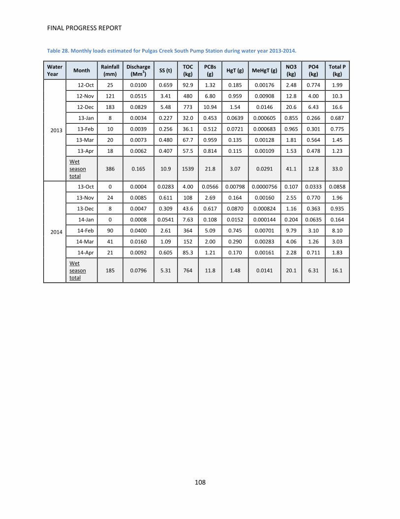
FINAL PROGRESS REPORT
108
Table 28. Monthly loads estimated for Pulgas Creek South Pump Station during water year 2013-2014.
Water Year Month Rainfall
(mm) Discharge
(Mm3) SS (t) TOC (kg)
PCBs (g) HgT (g) MeHgT (g) NO3
(kg) PO4 (kg)
Total P (kg)
2013
12-Oct 25 0.0100 0.659 92.9 1.32 0.185 0.00176 2.48 0.774 1.99
12-Nov 121 0.0515 3.41 480 6.80 0.959 0.00908 12.8 4.00 10.3
12-Dec 183 0.0829 5.48 773 10.94 1.54 0.0146 20.6 6.43 16.6
13-Jan 8 0.0034 0.227 32.0 0.453 0.0639 0.000605 0.855 0.266 0.687
13-Feb 10 0.0039 0.256 36.1 0.512 0.0721 0.000683 0.965 0.301 0.775
13-Mar 20 0.0073 0.480 67.7 0.959 0.135 0.00128 1.81 0.564 1.45
13-Apr 18 0.0062 0.407 57.5 0.814 0.115 0.00109 1.53 0.478 1.23
Wet season total
386 0.165 10.9 1539 21.8 3.07 0.0291 41.1 12.8 33.0
2014
13-Oct 0 0.0004 0.0283 4.00 0.0566 0.00798 0.0000756 0.107 0.0333 0.0858
13-Nov 24 0.0085 0.611 108 2.69 0.164 0.00160 2.55 0.770 1.96
13-Dec 8 0.0047 0.309 43.6 0.617 0.0870 0.000824 1.16 0.363 0.935
14-Jan 0 0.0008 0.0541 7.63 0.108 0.0152 0.000144 0.204 0.0635 0.164
14-Feb 90 0.0400 2.61 364 5.09 0.745 0.00701 9.79 3.10 8.10
14-Mar 41 0.0160 1.09 152 2.00 0.290 0.00283 4.06 1.26 3.03
14-Apr 21 0.0092 0.605 85.3 1.21 0.170 0.00161 2.28 0.711 1.83
Wet season total
185 0.0796 5.31 764 11.8 1.48 0.0141 20.1 6.31 16.1

FINAL PROGRESS REPORT
109
Attachment 1. Quality Assurance information Table A1: Summary of QA data at all sites. This table includes the top eight PAHs found commonly at all sites , the PBDE congeners that account for 75% of the sum of all PBDE congeners, the top nine PCB congeners found at all sites, and the pyrethroids that were detected at any site.
Analyte Unit AverageLabBlank
Detection Limit
(MDL) (range; mean)
Average Reporting Limit
(RL)
RSD of Lab
Duplicates (% range; % mean)
RSD of Field
Duplicates (% range; % mean)
Percent Recovery of CRM
(% range; % mean)
Percent Recovery of Matrix Spike (% range; %
mean)
Carbaryl ng/L 0 9.9-10; 10 20
75.71-75.71; 75.71
1.39-83.55; 42.47 NA
66.64-120.25; 94.99
Fipronil ng/L 0 0.5-5; 0.945 4.34 NA
0.00-141.42; 28.84 NA
51.52-150.00; 86.24
NH4 mg/L 0
0.015-0.04; 0.024 0.0486 NA
0.00-11.79; 4.47 NA
80.00-120.00; 102.41
NO3 mg/L 0
0.002-0.05;
0.0113 0.0488 0.00-0.00;
0.00 0.00-
42.43; 2.51 NA
90.00-105.00; 98.98
PO4 mg/L 0
0.0035-0.06;
0.00599 0.0112 0.00-1.61;
0.90 0.00-5.29;
1.51 NA
83.50-126.06; 97.94
Total P mg/L 0 0.007-0.1;
0.016 0.01 0.00-2.40;
0.79 0.00-
33.17; 3.90 NA
86.00-113.00; 97.30
SSC mg/L 0 0.23-6.8;
2.28 3 NA
0.00-85.48; 12.61
80.99-114.49; 100.72 NA
Benz(a)anthracenes/Chrysenes, C1- ng/L 0.245 0.0364-
75.5; 2.64 NA NA NA NA NA Benz(a)anthracenes/Chrysenes, C2- ng/L 0.177 0.046- NA NA NA NA NA

FINAL PROGRESS REPORT
110
Analyte Unit AverageLabBlank
Detection Limit
(MDL) (range; mean)
Average Reporting Limit
(RL)
RSD of Lab
Duplicates (% range; % mean)
RSD of Field
Duplicates (% range; % mean)
Percent Recovery of CRM
(% range; % mean)
Percent Recovery of Matrix Spike (% range; %
mean) 43.1; 1.98
Fluoranthene ng/L 0.152
0.0382-2.58; 0.446 NA NA NA NA NA
Fluoranthene/Pyrenes, C1- ng/L 0.531 0.103-
25.4; 2.08 NA NA NA NA NA
Fluorenes, C3- ng/L 1.42 0.0451-
29.4; 1.47 NA NA NA NA NA
Naphthalenes, C4- ng/L 1.86
0.0461-3.54; 0.751 NA NA NA NA NA
Phenanthrene/Anthracene, C4- ng/L 1.44 0.0891-
27.1; 2.72 NA NA NA NA NA
Pyrene ng/L 0.133
0.0376-5.96; 0.562 NA NA NA NA NA
PBDE 047 ng/L 0.0363
0.000368-0.000872; 0.000414 NA NA NA NA NA
PBDE 099 ng/L 0.0379
0.000472-0.0124; 0.00366 NA NA NA NA NA
PBDE 209 ng/L 0.101
0.0127-0.24;
0.0771 NA NA NA NA NA
PCB 087 ng/L 0.00147
0.000184-0.0337; 0.00142 NA NA NA NA NA

FINAL PROGRESS REPORT
111
Analyte Unit AverageLabBlank
Detection Limit
(MDL) (range; mean)
Average Reporting Limit
(RL)
RSD of Lab
Duplicates (% range; % mean)
RSD of Field
Duplicates (% range; % mean)
Percent Recovery of CRM
(% range; % mean)
Percent Recovery of Matrix Spike (% range; %
mean)
PCB 095 ng/L 0.0013
0.000184-0.0372; 0.0016 NA NA NA NA NA
PCB 110 ng/L 0.00184
0.000184-0.029;
0.00122 NA NA NA NA NA
PCB 138 ng/L 0.0018
0.000214-0.149;
0.00441 NA NA NA NA NA
PCB 149 ng/L 0.00101
0.00022-0.151;
0.00469 NA NA NA NA NA
PCB 151 ng/L 0.000445
0.000184-0.0195; 0.00115 NA NA NA NA NA
PCB 153 ng/L 0.00178
0.000209-0.132;
0.00392 NA NA NA NA NA
PCB 174 ng/L 0.0000338
0.000184-0.0118; 0.00106 NA NA NA NA NA
PCB 180 ng/L 0.000603
0.000184-0.00952; 0.000908 NA NA NA NA NA
Bifenthrin ng/L 0.0457 0.05-5.52;
0.761 1.53 NA NA NA NA
Cypermethrin ng/L 0 0.1-5.29;
0.815 1.53 NA NA NA NA

FINAL PROGRESS REPORT
112
Analyte Unit AverageLabBlank
Detection Limit
(MDL) (range; mean)
Average Reporting Limit
(RL)
RSD of Lab
Duplicates (% range; % mean)
RSD of Field
Duplicates (% range; % mean)
Percent Recovery of CRM
(% range; % mean)
Percent Recovery of Matrix Spike (% range; %
mean)
Delta/Tralomethrin ng/L 0.155 0.1-1; 0.258 3.05 NA NA NA NA
Total Cu ug/L 0
0.042-0.421; 0.114 0.527
0.20-2.68; 0.88
0.00-3.72; 1.06
100.66-106.15; 102.50
80.00-200.00; 97.76
Dissolved Cu ug/L 0
0.042-0.421; 0.096 0.5 NA
0.00-12.65; 3.92 NA
85.50-98.00; 92.24
Total Hg ng/L 0 0.2-2; 0.234 0.526
2.12-2.12; 2.12
0.00-63.15; 13.84
91.93-106.84; 99.17
92.99-119.87; 104.34
Total MeHg ng/L 0.00354 0.01-0.02;
0.0177 0.0401 0.97-5.87;
3.35 0.00-
37.52; 8.84 NA
58.99-137.27; 95.64
Total Se ug/L 0.0094
0.024-0.06;
0.0503 0.0925
0.29-26.96; 5.76
0.00-33.12; 6.97
92.56-103.84; 100.00
80.78-121.22; 95.67
Dissolved Se ug/L 0
0.024-0.06;
0.0523 0.124 6.18-6.18;
6.18 0.00-6.18;
3.03 NA
87.20-96.22; 91.35
TOC mg/L 0.0197 0.035-0.3;
0.249 0.481 NA 0.00-
15.71; 3.49 NA
0.03-123.00; 96.59

FINAL PROGRESS REPORT
113
Table A2: Field blank data from all sites.
Analyte Unit Average MDL RL Minimum Field
Blank Maximum Field Blank
Average Field Blank
Carbaryl ng/L 10 20 ND ND ND Fipronil ng/L 0.714 3.14 ND ND ND NO3 mg/L 0.0123 0.047 ND 0.039 0.00279 PO4 mg/L 0.00583 0.01 ND 0.008 0.001 Total P mg/L 0.00719 0.01 ND 0.057 0.00519 SSC mg/L 2 3 ND ND ND Acenaphthene ng/L 0.31 - ND ND ND Acenaphthylene ng/L 0.0803 - ND 0.0663 0.0133 Anthracene ng/L 0.143 - ND ND ND Benz(a)anthracene ng/L 0.0394 - ND 0.0406 0.00812 Benz(a)anthracenes/Chrysenes, C1- ng/L 0.0293 - ND 0.173 0.0814 Benz(a)anthracenes/Chrysenes, C2- ng/L 0.0515 - ND 0.393 0.186 Benz(a)anthracenes/Chrysenes, C3- ng/L 0.0457 - ND 0.389 0.174 Benz(a)anthracenes/Chrysenes, C4- ng/L 0.0478 - ND 1.03 0.329 Benzo(a)pyrene ng/L 0.111 - ND ND ND Benzo(b)fluoranthene ng/L 0.0509 - ND 0.121 0.0407 Benzo(e)pyrene ng/L 0.102 - ND 0.0695 0.0139 Benzo(g,h,i)perylene ng/L 0.0671 - ND ND ND Benzo(k)fluoranthene ng/L 0.11 - ND ND ND Chrysene ng/L 0.0407 - ND 0.151 0.0704 Dibenz(a,h)anthracene ng/L 0.0693 - ND ND ND Dibenzothiophene ng/L 0.0688 - ND 0.289 0.0974 Dibenzothiophenes, C1- ng/L 0.089 - ND ND ND Dibenzothiophenes, C2- ng/L 0.052 - 0.266 0.71 0.486 Dibenzothiophenes, C3- ng/L 0.0524 - 0.484 0.782 0.637 Dimethylnaphthalene, 2,6- ng/L 0.247 - ND 0.854 0.327

FINAL PROGRESS REPORT
114
Analyte Unit Average MDL RL Minimum Field
Blank Maximum Field Blank
Average Field Blank
Fluoranthene ng/L 0.0333 - 0.104 0.343 0.238 Fluoranthene/Pyrenes, C1- ng/L 0.113 - 0.0828 0.716 0.387 Fluorene ng/L 0.103 - ND 0.229 0.098 Fluorenes, C2- ng/L 0.122 - 1.39 3.5 2.37 Fluorenes, C3- ng/L 0.133 - 2.95 4.13 3.58 Indeno(1,2,3-c,d)pyrene ng/L 0.0417 - ND ND ND Methylnaphthalene, 2- ng/L 0.233 - ND 5.56 1.7 Methylphenanthrene, 1- ng/L 0.119 - ND 0.12 0.0419 Naphthalene ng/L 0.145 - 1.7 22.4 10.5 Naphthalenes, C1- ng/L 0.093 - ND 8.71 2.69 Naphthalenes, C3- ng/L 0.167 - 0.601 3.94 2.15 Perylene ng/L 0.116 - ND ND ND Phenanthrene ng/L 0.0885 - 0.436 0.717 0.543 Phenanthrene/Anthracene, C1- ng/L 0.119 - ND 0.533 0.256 Phenanthrene/Anthracene, C2- ng/L 0.068 - 0.0581 0.843 0.485 Pyrene ng/L 0.0323 - 0.0763 0.229 0.164 Trimethylnaphthalene, 2,3,5- ng/L 0.11 - ND 0.385 0.176 PBDE 007 ng/L 0.000474 - ND 0.00164 0.000328 PBDE 008 ng/L 0.000434 - ND 0.0013 0.00026 PBDE 010 ng/L 0.000561 - ND ND ND PBDE 011 ng/L - - - - - PBDE 012 ng/L 0.000417 - ND 0.000793 0.000159 PBDE 013 ng/L - - - - - PBDE 015 ng/L 0.000401 - ND 0.00416 0.000832 PBDE 017 ng/L 0.000483 - ND 0.0236 0.00503 PBDE 025 ng/L - - - - - PBDE 028 ng/L 0.000772 - ND 0.029 0.00609 PBDE 030 ng/L 0.000457 - ND ND ND

FINAL PROGRESS REPORT
115
Analyte Unit Average MDL RL Minimum Field
Blank Maximum Field Blank
Average Field Blank
PBDE 032 ng/L 0.00042 - ND ND ND PBDE 033 ng/L - - - - - PBDE 035 ng/L 0.000939 - ND ND ND PBDE 047 ng/L 0.000478 - 0.0156 1.04 0.266 PBDE 049 ng/L 0.0009 - ND 0.0863 0.0187 PBDE 051 ng/L 0.000521 - ND 0.00865 0.00173 PBDE 066 ng/L 0.00136 - ND 0.0494 0.00988 PBDE 071 ng/L 0.000579 - ND 0.0143 0.00286 PBDE 075 ng/L 0.00102 - ND ND ND PBDE 077 ng/L 0.000537 - ND ND ND PBDE 079 ng/L 0.000484 - ND ND ND PBDE 085 ng/L 0.00151 - ND 0.0578 0.0137 PBDE 099 ng/L 0.000743 - 0.0295 1.2 0.308 PBDE 100 ng/L 0.000564 - 0.00597 0.281 0.0726 PBDE 105 ng/L 0.0012 - ND ND ND PBDE 116 ng/L 0.00189 - ND 0.0113 0.00226 PBDE 119 ng/L 0.00109 - ND 0.00686 0.00149 PBDE 120 ng/L - - - - - PBDE 126 ng/L 0.000751 - ND 0.00121 0.000242 PBDE 128 ng/L 0.00495 - ND ND ND PBDE 140 ng/L 0.000817 - ND 0.00677 0.00154 PBDE 153 ng/L 0.000892 - 0.00334 0.135 0.0316 PBDE 155 ng/L 0.000608 - ND 0.00943 0.00207 PBDE 166 ng/L - - - - - PBDE 181 ng/L 0.00218 - ND ND ND PBDE 183 ng/L 0.00253 - ND 0.0437 0.00874 PBDE 190 ng/L 0.00454 - ND ND ND PBDE 197 ng/L 0.00387 - 0.00236 0.0973 0.0498

FINAL PROGRESS REPORT
116
Analyte Unit Average MDL RL Minimum Field
Blank Maximum Field Blank
Average Field Blank
PBDE 203 ng/L 0.00308 - ND 0.123 0.0266 PBDE 204 ng/L - - - - - PBDE 205 ng/L 0.00563 - ND ND ND PBDE 206 ng/L 0.0222 - ND 1.4 0.287 PBDE 207 ng/L 0.0177 - ND 2.33 0.488 PBDE 208 ng/L 0.0265 - ND 1.69 0.338 PBDE 209 ng/L 0.0512 - ND 22.9 4.99 PCB 008 ng/L 0.00134 - ND 0.0204 0.00303 PCB 018 ng/L 0.000722 - ND 0.109 0.0112 PCB 020 ng/L - - - - - PCB 021 ng/L - - - - - PCB 028 ng/L 0.000465 - 0.00121 0.065 0.00967 PCB 030 ng/L - - - - - PCB 031 ng/L 0.000515 - ND 0.0477 0.00667 PCB 033 ng/L 0.000523 - ND 0.0115 0.00202 PCB 044 ng/L 0.000904 - ND 0.0494 0.00645 PCB 047 ng/L - - - - - PCB 049 ng/L 0.00102 - ND 0.0245 0.00277 PCB 052 ng/L 0.000668 - ND 0.0431 0.0062 PCB 056 ng/L 0.00056 - ND 0.00776 0.00112 PCB 060 ng/L 0.000608 - ND 0.0013 0.000306 PCB 061 ng/L - - - - - PCB 065 ng/L - - - - - PCB 066 ng/L 0.000699 - ND 0.00817 0.00176 PCB 069 ng/L - - - - - PCB 070 ng/L 0.000534 - 0.00121 0.02 0.00467 PCB 074 ng/L - - - - - PCB 076 ng/L - - - - -

FINAL PROGRESS REPORT
117
Analyte Unit Average MDL RL Minimum Field
Blank Maximum Field Blank
Average Field Blank
PCB 083 ng/L - - - - - PCB 086 ng/L - - - - - PCB 087 ng/L 0.000815 - ND 0.00809 0.00283 PCB 090 ng/L - - - - - PCB 093 ng/L - - - - - PCB 095 ng/L 0.000997 - ND 0.0115 0.00335 PCB 097 ng/L - - - - - PCB 098 ng/L - - - - - PCB 099 ng/L 0.000777 - ND 0.00753 0.00189 PCB 100 ng/L - - - - - PCB 101 ng/L 0.00155 - ND 0.00392 0.00246 PCB 102 ng/L - - - - - PCB 105 ng/L 0.000877 - ND 0.0033 0.000927 PCB 108 ng/L - - - - - PCB 110 ng/L 0.00099 - ND 0.0113 0.00416 PCB 113 ng/L - - - - - PCB 115 ng/L - - - - - PCB 118 ng/L 0.000824 - ND 0.00796 0.00237 PCB 119 ng/L - - - - - PCB 125 ng/L - - - - - PCB 128 ng/L 0.000753 - ND 0.00127 0.000397 PCB 129 ng/L - - - - - PCB 132 ng/L 0.00104 - ND 0.00272 0.00113 PCB 135 ng/L - - - - - PCB 138 ng/L 0.00124 - ND 0.012 0.00353 PCB 141 ng/L 0.000792 - ND 0.00096 0.000246 PCB 147 ng/L - - - - - PCB 149 ng/L 0.00126 - ND 0.00828 0.00237

FINAL PROGRESS REPORT
118
Analyte Unit Average MDL RL Minimum Field
Blank Maximum Field Blank
Average Field Blank
PCB 151 ng/L 0.000754 - ND 0.00463 0.00103 PCB 153 ng/L 0.00193 - ND 0.00341 0.00154 PCB 154 ng/L - - - - - PCB 156 ng/L 0.000731 - ND 0.000581 0.000132 PCB 157 ng/L - - - - - PCB 158 ng/L 0.000607 - ND 0.000602 0.000117 PCB 160 ng/L - - - - - PCB 163 ng/L - - - - - PCB 166 ng/L - - - - - PCB 168 ng/L - - - - - PCB 170 ng/L 0.000802 - ND 0.00131 0.000401 PCB 174 ng/L 0.000818 - ND 0.00139 0.000347 PCB 177 ng/L 0.000731 - ND 0.000988 0.000278 PCB 180 ng/L 0.00137 - ND 0.00274 0.000713 PCB 183 ng/L 0.000725 - ND 0.00208 0.000442 PCB 185 ng/L - - - - - PCB 187 ng/L 0.00096 - ND 0.00509 0.000853 PCB 193 ng/L - - - - - PCB 194 ng/L 0.000832 - ND 0.000731 0.0000522 PCB 195 ng/L 0.000803 - ND 0.000261 0.0000186 PCB 201 ng/L 0.000633 - ND ND ND PCB 203 ng/L 0.000903 - ND ND ND Allethrin ng/L 0.465 1.5 ND ND ND Bifenthrin ng/L 0.202 1.5 ND ND ND Cyfluthrin, total ng/L 1.14 1.5 ND ND ND Cyhalothrin,lambda, total ng/L 0.24 1.5 ND 0.11 0.0157 Cypermethrin, total ng/L 0.276 1.5 ND ND ND Delta/Tralomethrin ng/L 0.21 3 ND ND ND

FINAL PROGRESS REPORT
119
Analyte Unit Average MDL RL Minimum Field
Blank Maximum Field Blank
Average Field Blank
Esfenvalerate/Fenvalerate, total ng/L 0.254 3 ND ND ND Fenpropathrin ng/L 0.386 1.5 ND ND ND Permethrin, total ng/L 1.37 15 ND ND ND Phenothrin ng/L 0.525 - ND ND ND Prallethrin ng/L 7.02 - ND ND ND Resmethrin ng/L 0.653 - ND ND ND Total Cu ug/L 0.066 0.444 ND 1.4 0.45 Dissolved Cu ug/L 0.066 0.444 ND 1.4 0.297 Total Hg ng/L 0.199 0.482 ND 4.4 0.271 Total MeHg ng/L 0.0192 0.04 ND 0.021 0.00162 Dissolved Se ug/L 0.0549 0.096 ND ND ND Total Se ug/L 0.0549 0.096 ND ND ND Total Hardness (calc) mg/L 1.46 4.3 ND ND ND TOC mg/L 0.3 0.5 ND ND ND

FINAL PROGRESS REPORT
120
Table A3: Average RSD of field and lab duplicates at each site.
San Leandro
Creek East Sunnyvale
Channel Lower Marsh
Creek Guadalupe
River Richmond
Pump Station Pulgas Creek
Analyte
Avg Field RSD
Avg Lab RSD
Avg Field RSD
Avg Lab RSD
Avg Field RSD
Avg Lab RSD
Avg Field RSD
Avg Lab RSD
Avg Field RSD
Avg Lab RSD
Avg Field RSD
Avg Lab RSD
Carbaryl - - - - - - 83.50% 75.70% - - 1.40% -
Fipronil 53.00% - 31.40% - 9.20% - 10.90% - 10.90% - - -
NO3 0.00% 0.00% 9.90% 0.00% 0.50% - 0.00% 0.00% 1.80% - 0.40% -
PO4 0.50% 0.80% 1.90% 0.90% 0.30% - 1.40% 1.10% 1.50% - 3.70% -
Total P 3.60% 0.00% 0.90% 0.00% 3.00% 2.40% 12.40% 0.00% 1.70% - 2.70% -
SSC 11.00% - 6.20% - 11.90% - 36.20% - 12.40% - 10.00% -
Acenaphthene 20.10% - 6.30% 3.70% - - 10.00% 0.40% 2.10% 1.50% - -
Acenaphthylene 10.70% - 8.50% 5.00% - - 31.80% 18.10% 5.70% 5.50% - -
Anthracene 14.20% - 14.10% 5.00% 43.40% - 39.10% 23.40% 5.60% 4.10% - -
Benz(a)anthracene 15.30% - 18.70% 11.40% - - - - - - - -
Benz(a)anthracenes/Chrysenes, C1- 5.70% - 6.70% 2.30% 2.90% - 17.30% 6.80% 1.30% 1.30% - -

FINAL PROGRESS REPORT
121
San Leandro
Creek East Sunnyvale
Channel Lower Marsh
Creek Guadalupe
River Richmond
Pump Station Pulgas Creek
Analyte
Avg Field RSD
Avg Lab RSD
Avg Field RSD
Avg Lab RSD
Avg Field RSD
Avg Lab RSD
Avg Field RSD
Avg Lab RSD
Avg Field RSD
Avg Lab RSD
Avg Field RSD
Avg Lab RSD
Benz(a)anthracenes/Chrysenes, C2- 4.30% - 7.80% 7.70% 6.00% - 19.00% 16.40% 2.80% 1.70% - -
Benz(a)anthracenes/Chrysenes, C3- 23.60% - 15.80% 13.50% 11.10% - 40.20% 8.90% 2.50% 3.40% - -
Benz(a)anthracenes/Chrysenes, C4- 5.90% - 23.90% 26.40% 10.60% - 16.70% 7.00% 4.00% 0.40% - -
Benzo(a)pyrene 16.70% - 11.80% 5.10% 20.80% - 23.60% 6.50% 3.60% 4.80% - -
Benzo(b)fluoranthene 9.30% - 9.70% 6.70% 26.60% - 17.50% 5.20% 4.60% 4.70% - -
Benzo(e)pyrene 13.50% - 7.50% 7.20% 9.90% - 28.40% 5.90% 2.00% 1.00% - -
Benzo(g,h,i)perylene 16.60% - 5.50% 0.60% 4.60% - 14.20% 5.30% 3.50% 3.20% - -
Benzo(k)fluoranthene 36.40% - 20.60% 1.80% - - 33.00% 2.80% - - - -
Chrysene 8.40% - 8.90% 3.50% 9.50% - 19.00% 7.50% 4.00% 5.00% - -
Dibenz(a,h)anthracene 39.90% - 25.20% 10.90% - - - - 2.00% 1.20% - -
Dibenzothiophene - - 7.20% 5.20% - - 15.90% 13.00% - - - -
Dibenzothiophenes, C1- 8.90% - 5.90% 3.90% 5.10% - 24.60% 2.90% 7.00% 2.60% - -

FINAL PROGRESS REPORT
122
San Leandro
Creek East Sunnyvale
Channel Lower Marsh
Creek Guadalupe
River Richmond
Pump Station Pulgas Creek
Analyte
Avg Field RSD
Avg Lab RSD
Avg Field RSD
Avg Lab RSD
Avg Field RSD
Avg Lab RSD
Avg Field RSD
Avg Lab RSD
Avg Field RSD
Avg Lab RSD
Avg Field RSD
Avg Lab RSD
Dibenzothiophenes, C2- 4.50% - 7.20% 5.70% 10.20% - 12.20% 2.90% 4.40% 4.90% - -
Dibenzothiophenes, C3- 4.80% - 8.90% 2.30% 8.00% - 14.70% 0.80% 3.70% 3.80% - -
Dimethylnaphthalene, 2,6- 22.20% - 5.10% 3.70% 0.40% - 12.20% 13.80% 4.20% 3.90% - -
Fluoranthene 16.00% - 10.60% 3.30% 33.20% - 17.20% 16.00% 5.50% 3.50% - -
Fluoranthene/Pyrenes, C1- 16.30% - 9.90% 2.80% 8.70% - 17.40% 2.90% 2.00% 2.30% - -
Fluorene 15.30% - 15.00% 4.00% - - 15.80% 9.10% 2.70% 2.90% - -
Fluorenes, C2- 14.00% - 7.30% 8.90% 0.80% - 9.40% 1.20% 3.30% 4.30% - -
Fluorenes, C3- 7.00% - 11.30% 2.80% 9.00% - 12.30% 0.10% 2.00% 2.50% - -
Indeno(1,2,3-c,d)pyrene 21.90% - 8.80% 2.30% 14.90% - 18.10% 5.30% 6.70% 6.70% - -
Methylnaphthalene, 2- 9.30% - 4.10% 2.60% 2.10% - 10.60% 6.30% 2.40% 1.90% - -
Methylphenanthrene, 1- 16.70% - 14.40% 9.50% 11.60% - 14.60% 10.70% 0.80% 0.80% - -
Naphthalene 10.30% - 5.20% 1.90% 3.20% - 2.10% 3.80% 2.40% 0.50% - -
Naphthalenes, C1- 14.50% - 6.40% 3.70% 0.50% - 7.50% 5.70% 2.30% 1.70% - -
Naphthalenes, C3- 17.20% - 7.80% 7.90% 0.60% - 8.90% 11.20% 5.30% 5.80% - -

FINAL PROGRESS REPORT
123
San Leandro
Creek East Sunnyvale
Channel Lower Marsh
Creek Guadalupe
River Richmond
Pump Station Pulgas Creek
Analyte
Avg Field RSD
Avg Lab RSD
Avg Field RSD
Avg Lab RSD
Avg Field RSD
Avg Lab RSD
Avg Field RSD
Avg Lab RSD
Avg Field RSD
Avg Lab RSD
Avg Field RSD
Avg Lab RSD
Perylene 17.60% - 13.70% 5.80% 5.00% - 25.60% 8.60% 3.50% 4.30% - -
Phenanthrene 5.80% - 20.20% 5.30% 29.00% - 21.30% 26.50% 2.50% 2.10% - -
Phenanthrene/Anthracene, C1- 28.70% - 10.30% 3.00% 13.70% - 13.00% 0.20% 2.60% 2.00% - -
Phenanthrene/Anthracene, C2- 15.60% - 9.10% 7.30% 7.10% - 12.90% 8.10% 2.80% 2.80% - -
Pyrene 16.70% - 9.00% 3.00% 19.50% - 19.20% 14.40% 4.60% 3.90% - -
Trimethylnaphthalene, 2,3,5- 22.10% - 7.80% 3.40% 2.30% - 17.60% 9.00% 3.30% 4.50% - -
PBDE 007 - - - - - - - 11.20% 15.40% 15.60% 2.00% 2.00%
PBDE 008 - - - - - - - - - - - -
PBDE 010 - - - - - - - - - - - -
PBDE 012 - - - - - - - - - - - -
PBDE 015 11.20% 9.50% 0.70% - - - 3.20% 4.30% 12.30% 15.40% 7.50% 7.50%
PBDE 017 - - - - - - - - - - - -
PBDE 028 - - - - - - - - - - - -
PBDE 030 - - - - - - - - - - - -

FINAL PROGRESS REPORT
124
San Leandro
Creek East Sunnyvale
Channel Lower Marsh
Creek Guadalupe
River Richmond
Pump Station Pulgas Creek
Analyte
Avg Field RSD
Avg Lab RSD
Avg Field RSD
Avg Lab RSD
Avg Field RSD
Avg Lab RSD
Avg Field RSD
Avg Lab RSD
Avg Field RSD
Avg Lab RSD
Avg Field RSD
Avg Lab RSD
PBDE 032 - - - - - - - - - - - -
PBDE 035 - - - - - - - - - - - -
PBDE 047 8.30% 1.20% 4.40% - - - 13.80% 18.20% 6.40% 0.70% 4.60% 4.60%
PBDE 049 4.10% 0.70% 1.50% - - - 10.20% 8.60% 5.40% 3.20% 12.40% 12.40%
PBDE 051 5.70% 5.70% 0.70% - - - - - 10.50% 6.70% 15.30% 15.30%
PBDE 066 2.00% 0.50% 1.10% - - - 13.80% 14.10% 6.30% 2.80% 8.40% 8.40%
PBDE 071 1.90% 1.90% 2.30% - - - - - 18.20% 19.60% 32.70% 32.70%
PBDE 075 0.70% 0.70% 9.80% - - - - - 0.80% 0.60% 22.00% 22.00%
PBDE 077 15.80% 15.80% - - - - - - - - - -
PBDE 079 16.40% 16.40% - - - - - - 21.80% 15.60% - -
PBDE 085 12.50% 5.20% 5.00% - - - 4.60% 5.70% 12.40% 3.70% 2.90% 2.90%
PBDE 099 8.90% 3.90% 3.30% - - - 8.10% 9.90% 9.30% 2.40% 4.80% 4.80%
PBDE 100 5.20% 0.30% 3.80% - - - 9.20% 11.70% 8.90% 1.10% 6.00% 6.00%
PBDE 105 - - - - - - - - - - - -

FINAL PROGRESS REPORT
125
San Leandro
Creek East Sunnyvale
Channel Lower Marsh
Creek Guadalupe
River Richmond
Pump Station Pulgas Creek
Analyte
Avg Field RSD
Avg Lab RSD
Avg Field RSD
Avg Lab RSD
Avg Field RSD
Avg Lab RSD
Avg Field RSD
Avg Lab RSD
Avg Field RSD
Avg Lab RSD
Avg Field RSD
Avg Lab RSD
PBDE 116 - - - - - - - - - - - -
PBDE 119 - - - - - - - - - - - -
PBDE 126 - - - - - - - - - - - -
PBDE 128 - - - - - - - - - - - -
PBDE 140 - - 30.00% - - - 12.10% 12.50% 15.70% 2.70% 9.80% 9.80%
PBDE 153 11.20% 6.60% 9.90% - - - 6.20% 7.10% 9.50% 3.80% 3.50% 3.50%
PBDE 155 9.20% 12.50% - - - - 6.40% 7.80% 17.60% 3.70% 6.00% 6.00%
PBDE 181 - - - - - - - - - - - -
PBDE 183 16.40% 1.50% 18.50% - - - 27.40% 32.60% 15.40% 6.10% 11.00% 11.00%
PBDE 190 - - - - - - - - - - 1.70% 1.70%
PBDE 197 34.70% 12.30% 15.80% - - - - - - - - -
PBDE 203 25.10% 17.60% 14.80% - - - - 3.30% 22.40% 12.70% 4.60% 4.60%
PBDE 205 - - - - - - - - - - - -
PBDE 206 18.40% 23.90% 10.60% - - - 6.10% 7.60% 21.90% 10.50% 37.30% 37.30%
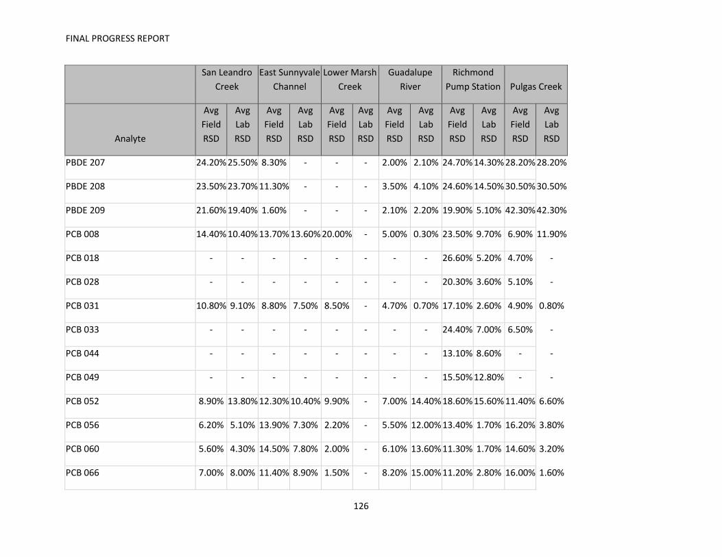
FINAL PROGRESS REPORT
126
San Leandro
Creek East Sunnyvale
Channel Lower Marsh
Creek Guadalupe
River Richmond
Pump Station Pulgas Creek
Analyte
Avg Field RSD
Avg Lab RSD
Avg Field RSD
Avg Lab RSD
Avg Field RSD
Avg Lab RSD
Avg Field RSD
Avg Lab RSD
Avg Field RSD
Avg Lab RSD
Avg Field RSD
Avg Lab RSD
PBDE 207 24.20% 25.50% 8.30% - - - 2.00% 2.10% 24.70% 14.30% 28.20% 28.20%
PBDE 208 23.50% 23.70% 11.30% - - - 3.50% 4.10% 24.60% 14.50% 30.50% 30.50%
PBDE 209 21.60% 19.40% 1.60% - - - 2.10% 2.20% 19.90% 5.10% 42.30% 42.30%
PCB 008 14.40% 10.40% 13.70% 13.60% 20.00% - 5.00% 0.30% 23.50% 9.70% 6.90% 11.90%
PCB 018 - - - - - - - - 26.60% 5.20% 4.70% -
PCB 028 - - - - - - - - 20.30% 3.60% 5.10% -
PCB 031 10.80% 9.10% 8.80% 7.50% 8.50% - 4.70% 0.70% 17.10% 2.60% 4.90% 0.80%
PCB 033 - - - - - - - - 24.40% 7.00% 6.50% -
PCB 044 - - - - - - - - 13.10% 8.60% - -
PCB 049 - - - - - - - - 15.50% 12.80% - -
PCB 052 8.90% 13.80% 12.30% 10.40% 9.90% - 7.00% 14.40% 18.60% 15.60% 11.40% 6.60%
PCB 056 6.20% 5.10% 13.90% 7.30% 2.20% - 5.50% 12.00% 13.40% 1.70% 16.20% 3.80%
PCB 060 5.60% 4.30% 14.50% 7.80% 2.00% - 6.10% 13.60% 11.30% 1.70% 14.60% 3.20%
PCB 066 7.00% 8.00% 11.40% 8.90% 1.50% - 8.20% 15.00% 11.20% 2.80% 16.00% 1.60%

FINAL PROGRESS REPORT
127
San Leandro
Creek East Sunnyvale
Channel Lower Marsh
Creek Guadalupe
River Richmond
Pump Station Pulgas Creek
Analyte
Avg Field RSD
Avg Lab RSD
Avg Field RSD
Avg Lab RSD
Avg Field RSD
Avg Lab RSD
Avg Field RSD
Avg Lab RSD
Avg Field RSD
Avg Lab RSD
Avg Field RSD
Avg Lab RSD
PCB 070 - - - - - - - - 6.00% 9.90% - -
PCB 087 - - - - - - - - 18.40% 22.40% 9.30% -
PCB 095 - - - - - - - - 21.10% 29.80% 16.10% -
PCB 099 - - - - - - - - 20.60% 24.70% 22.30% -
PCB 101 - - - - - - - - 17.10% 23.90% 20.10% -
PCB 105 7.40% 7.90% 19.30% 11.00% 13.40% - 7.70% 19.20% 14.90% 11.40% 17.30% 22.50%
PCB 110 - - - - - - - - 16.60% 20.90% 11.00% -
PCB 118 7.70% 8.60% 21.00% 8.70% 15.00% - 8.10% 20.80% 15.20% 13.60% 16.30% 27.90%
PCB 128 19.80% 19.80% - - - - - - 7.20% 15.00% 3.30% -
PCB 132 9.70% 9.20% 20.00% 4.70% 18.50% - 11.80% 25.80% 13.20% 18.40% 5.30% 11.40%
PCB 138 - - - - - - - - 6.60% 10.80% 1.40% -
PCB 141 9.40% 10.30% 19.40% 3.50% 14.80% - 14.00% 22.90% 15.50% 15.60% 7.70% 15.90%
PCB 149 - - - - - - - - 4.80% 10.40% 3.90% -
PCB 151 - - - - - - - - 3.00% 5.90% 3.50% -

FINAL PROGRESS REPORT
128
San Leandro
Creek East Sunnyvale
Channel Lower Marsh
Creek Guadalupe
River Richmond
Pump Station Pulgas Creek
Analyte
Avg Field RSD
Avg Lab RSD
Avg Field RSD
Avg Lab RSD
Avg Field RSD
Avg Lab RSD
Avg Field RSD
Avg Lab RSD
Avg Field RSD
Avg Lab RSD
Avg Field RSD
Avg Lab RSD
PCB 153 - - - - - - - - 6.40% 7.60% 2.70% -
PCB 156 - - - - - - - - 8.00% 18.60% - -
PCB 158 8.90% 11.00% 18.50% 3.80% 16.70% - 11.10% 24.80% 15.60% 16.00% 9.40% 16.70%
PCB 170 7.30% 4.70% 15.90% 1.40% 11.30% - 13.20% 24.70% 20.80% 7.90% 5.30% 7.70%
PCB 174 5.60% 1.70% 14.20% 2.20% 11.50% - 21.80% 36.30% 13.80% 1.50% 6.30% 7.20%
PCB 177 6.00% 3.70% 13.30% 3.40% 18.90% - 20.10% - 16.60% 4.30% 4.90% 6.00%
PCB 180 - - - - - - 23.70% 29.50% 15.00% 4.40% - -
PCB 183 - - - - - - 33.10% 31.60% 13.40% 5.50% - -
PCB 187 5.20% 3.80% 11.00% 3.90% 6.40% - 23.80% 34.90% 15.00% 5.00% 8.60% 10.50%
PCB 194 7.40% 3.30% 19.00% 5.60% 14.40% - 16.10% 38.70% 22.70% 12.20% 5.90% 8.20%
PCB 195 5.50% 2.00% 18.10% 3.40% 29.70% - 15.30% 26.90% 24.80% 12.70% 4.30% 3.80%
PCB 201 8.80% 2.40% 13.20% 1.10% 10.10% - 23.30% - 13.20% 6.80% 8.00% 8.20%
PCB 203 7.70% 6.70% 15.50% 5.40% 14.30% - 18.20% 44.10% 17.80% 17.10% 9.60% 12.90%
Allethrin - - - - - - - - - - - -
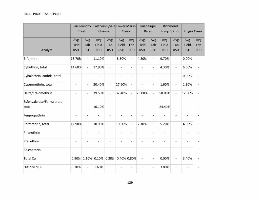
FINAL PROGRESS REPORT
129
San Leandro
Creek East Sunnyvale
Channel Lower Marsh
Creek Guadalupe
River Richmond
Pump Station Pulgas Creek
Analyte
Avg Field RSD
Avg Lab RSD
Avg Field RSD
Avg Lab RSD
Avg Field RSD
Avg Lab RSD
Avg Field RSD
Avg Lab RSD
Avg Field RSD
Avg Lab RSD
Avg Field RSD
Avg Lab RSD
Bifenthrin 18.70% - 11.10% - 8.50% - 4.80% - 9.70% - 0.00% -
Cyfluthrin, total 14.60% - 17.90% - - - - - 4.30% - 6.60% -
Cyhalothrin,lambda, total - - - - - - - - - - 0.00% -
Cypermethrin, total - - 30.40% - 27.60% - - - 1.60% - 1.30% -
Delta/Tralomethrin - - 39.50% - 32.40% - 23.00% - 58.00% - 12.90% -
Esfenvalerate/Fenvalerate, total - - 10.10% - - - - - 24.40% - - -
Fenpropathrin - - - - - - - - - - - -
Permethrin, total 12.90% - 10.90% - 10.60% - 2.10% - 5.20% - 4.00% -
Phenothrin - - - - - - - - - - - -
Prallethrin - - - - - - - - - - - -
Resmethrin - - - - - - - - - - - -
Total Cu 0.90% 1.10% 0.10% 0.20% 0.40% 0.80% - - 0.00% - 3.40% -
Dissolved Cu 6.30% - 1.60% - - - - - 3.80% - - -

FINAL PROGRESS REPORT
130
San Leandro
Creek East Sunnyvale
Channel Lower Marsh
Creek Guadalupe
River Richmond
Pump Station Pulgas Creek
Analyte
Avg Field RSD
Avg Lab RSD
Avg Field RSD
Avg Lab RSD
Avg Field RSD
Avg Lab RSD
Avg Field RSD
Avg Lab RSD
Avg Field RSD
Avg Lab RSD
Avg Field RSD
Avg Lab RSD
Total Hg 18.70% 2.10% 11.80% - 4.50% - 12.30% - 9.70% - 16.90% -
Total MeHg 10.00% 4.10% 11.90% - 2.70% - 10.60% 2.60% 10.70% - 1.40% -
Dissolved Se 3.10% 6.20% 1.60% - - - - - 5.20% - - -
Total Se 11.60% 10.10% 0.00% - 4.10% 1.50% 1.40% 1.40% 0.00% - 6.40% -
Total Hardness (calc) 1.20% - 8.30% - - - - - 0.00% - 6.30% -
TOC 1.50% - 3.00% - 3.80% - 6.10% - 6.40% - 1.50% -

FINAL PROGRESS REPORT
131
Attachment 2. Intercomparison Studies
Due to the change in analytical labs for 2013 and 2014 from those used previously in loading studies, a limited number of split samples were analyzed for intercomparison with results from laboratories contracted in previous years.
In general, the intra-lab variation from replicate analyses performed on these samples for both the current and previous contract labs, was much smaller than the inter-lab variation. This is to be expected; analytical biases (e.g., from mis-calibration, incomplete extraction, matrix interferences, etc.) will tend to recur and be more consistent within a lab than among labs. Even if both labs perform within typical acceptance limits for CRMs or other performance tests, the net difference between labs can sometimes be exacerbated by biases in opposite directions, or interferences present in specific field matrices but not reference materials, and in limited studies, it may be possible only to estimate a typical difference, not establish which lab’s results are more accurate. Differences in results between years and between sites analyzed by different labs that are smaller than or similar to the inter-lab measurement differences may not be real or significant and may only reflect measurement differences between labs.
Even in larger intercomparison exercises with multiple labs, there is no assurance provided that the certified or consensus value is absolutely accurate, only a weight of evidence that more or most labs get a similar result. Such a consensus may in part reflect a common bias among labs encountering a similar interference or bias of choosing a particular extraction or analytical method.
The following section will discuss results on split samples analyzed for this project in 2013 and 2014 for various analytes. In most cases the differences among labs were within common precision acceptance limits (e.g., 25% RPD for intra-lab replicates for trace metals in RMP or SWAMP) or within the expected combined (propagated) error for separate measurements of recovery (e.g. within 25% of target values for 2 independent labs for reference materials or matrix spikes for trace elements; propagated error = square root ((25%)^2+ (25%)^2 ) = ~35% ). In cases where the results between labs show a consistent bias, it may be possible to adjust for the bias in evaluating interannual or inter-site differences, but in cases where the inter-lab differences appear more randomly distributed, smaller interannual or inter-site differences may not be distinguishable from measurement uncertainty.
In cases where more random or less systematic differences were found between the labs’ results, it is often difficult to diagnose the cause without extensive investigation. Causes of the discrepancies may be particular to specific samples, or sporadic and hard to reproduce. However, because the data in this study are compiled to develop overall pictures of concentrations and loads from the various watersheds, the impact of measurement errors or variations in any individual samples is lessened; random errors will partially offset and the aggregate statistics will reasonably allow estimation of the central tendency of the data. For many of the analytes, the results were often in good agreement (near a 1:1 line) for all but 1 of the split sample pairs, so the data can, in many cases, be compared with acknowledgement of measurement uncertainty but without requiring adjustment, which is suitable only for cases of systematic bias. Results for specific analytes are discussed below.

FINAL PROGRESS REPORT
132
Trace Elements
Copper Copper was measured by Caltest (the “Target Lab”) in 2013 and 2014, and by Brooks Rand (the “IC Lab”) in previous years. Three samples each of dissolved and total copper were split and analyzed by both labs in the course of the study. For both labs, the within lab RPDs were within 5% or better for these split samples, suggesting that individually, neither of the labs had noticeable issues with subsampling the provided samples uniformly for replicate analysis. In general, the IC lab reported concentrations higher than the target lab for any given sample (Figure 9). For dissolved copper, the average difference in slope (fitting a linear regression through the origin, vs. an “ideal” 1:1 line) was 28%, and for total copper, the average difference in slope was 15%. For individual result pairs, the target lab result was always lower, ranging 65% to 89% (average 74%) of the IC lab result for dissolved samples and 83% to 95% (average 87%) for total samples; average RPD was 31% for dissolved copper, and 14% for total copper. These data hint at a systematic bias, but because of the small number of samples in the comparison and differences between labs within or nearly within common acceptance limits for within lab variation (e.g., 25% RPD for metals) more evidence of a systematic bias would be recommended before attempting to develop an adjustment factor between labs.
Figure 9 Target versus IC lab dissolved and total copper in split water samples for 2013 to 2014.
y = 0.72x
y = 0.85x
0
5
10
15
0 5 10 15
Targ
et La
b Co
pper
IC Lab Copper
Diss Copper

FINAL PROGRESS REPORT
133
Total Mercury Total mercury was measured by Caltest (the “Target Lab”) in 2013 and 2014, and by Moss Landing Marine Labs (the “IC Lab”) in previous years. Seven total (unfiltered) water samples were split and analyzed for total mercury by both labs in the course of the study. For both labs, none of these split samples were analyzed as lab replicates, but precision on lab replicate analyses averaged 16% RSD in 2014 for the target lab and 3% in 2014 for the IC lab. Similar to copper, the IC lab generally reported concentrations higher than the target lab for any given sample (Figure 10), although the bias is less consistent. For total mercury, the target lab result ranged 51% to 105% (average 82%) of the IC lab result; the average RPD was 25%. Much of this difference was driven by a single result pair in 2014, where the IC lab result was nearly double that of the target laboratory; without that pair, the slope would have been near 1:1 (1.03), so correction is not warranted given the overall deviation depending largely on that one sample pair.
Figure 10 Target versus IC lab total mercury in split water samples for 2013 to 2014.
y = 0.82x
0
0.05
0.1
0.15
0.00 0.05 0.10 0.15
Targ
et La
b M
ercu
ry
IC Lab Mercury
Total Mercury

FINAL PROGRESS REPORT
134
Methylmercury Methyl mercury was measured by Caltest (the “Target Lab”) in 2013 and 2014, and by Moss Landing Marine Labs (the “IC Lab”) in previous years. Four total (unfiltered) water samples were split and analyzed for methylmercury by both labs in the course of the study. Only the IC lab analyzed one of these split samples directly in lab replicates, with <1% RSD, but the target lab also had acceptable precision with average 16% RSD in 2014 for other samples in the project. Unlike the other metals, the results for the IC lab averaged slightly lower than the target lab (Figure 11). For methylmercury, the target lab ranged 90% to 132% (average 105%) of the IC lab result. The average RPD was 12%, with some points both above and below the 1:1 line. Similar to copper, the differences are neither large enough nor consistent enough to warrant a correction factor.
Figure 11 Target versus IC lab methylmercury in split water samples for 2013 to 2014.
y = 1.05x
0
0.2
0.4
0.6
0.00 0.20 0.40 0.60
Targ
et La
b M
ethy
lmer
cury
IC Lab Methylmercury
Methylmercury

FINAL PROGRESS REPORT
135
Selenium Selenium was measured by Caltest (the “Target Lab”) in 2013 and 2014, and by Brooks Rand (the “IC Lab”) in previous years. Two samples each of dissolved and total selenium were split and analyzed by both labs in the course of the study. For both labs, the within lab replicate RPDs were good, within 10% or better for these split samples. In general, the IC lab reported concentrations very slightly higher than the target lab for any given sample (Figure 12), but results were nearly identical among labs, and very similar between dissolved and total phase for any given sampling event. For dissolved selenium, the target lab results were 89% to 97% (average 92%) of the IC lab, and for total selenium 88% to 98% (average 95%). Averages of individual result pair RPDs were 9% for dissolved selenium, and 5% for total selenium. Corrections for selenium are clearly not warranted given the very good agreement.
Figure 12 Target versus IC lab dissolved and total selenium in split water samples for 2013 to 2014.
y = 0.96x
y = 0.97x
0
1
2
3
0 1 2 3
Targ
et La
b Se
leni
um
IC Lab Selenium
Diss Selenium
Total Selenium

FINAL PROGRESS REPORT
136
Hardness Hardness was measured by Caltest (the “Target Lab”) in 2013 and 2014, and by Brooks Rand (the “IC Lab”) in previous years by a calculation from Ca and Mg concentrations. Three samples were split for analysis by both labs in the course of the study. For the target lab, the within lab replicate RPDs or RSDs were 6% to 12% for these split samples, and for the IC lab 3% on the one sample they analyzed in replicate. There was no consistent bias, with the target lab reporting 85% to 116% (average 100%) of the IC lab result. Although recovery errors in lab control samples (a clean lab matrix) by the target lab were generally within 10% or better of the target value, for field sample matrix spikes, recoveries were highly variable, as low as 30% recovery (70% error), averaging over 20% error. The moderately large average recovery error and sporadic large excursions suggest uncertainties in the target lab hardness data, leading 2013 results to be censored (although raw results remain in the database, and are plotted in Figure 13 here). The IC lab did not report recovery on hardness directly, but recovery was good on Ca and Mg, with modest errors (from 8% to 12%). Given a lack of consistent bias, a correction factor is not warranted for hardness measurements.
Figure 13 Target versus IC lab hardness in split water samples for 2013 to 2014.
y = 1.11x
0
100
200
300
400
0 100 200 300 400
Targ
et La
b Ha
rdne
ss
IC Lab Hardness (mg/L CaCO3 equiv)

FINAL PROGRESS REPORT
137
Suspended Sediment Concentration Suspended sediment concentration (SSC) was measured by Caltest (the “Target Lab”) in 2013 and 2014, and by EBMUD (the “IC Lab”) in previous years. Three samples were split for analysis by both labs in the course of the study. For the target lab, the lab replicate RSDs were 6% to 12% for these split samples, and for the IC lab 3% on the one sample they analyzed in replicate. There was no consistent bias between labs (Figure 14). The target lab reported results 41% to 150% (average 101%) those of the IC lab, with the largest relative differences on the lower concentration samples. Recoveries on LCS samples by the target lab were within 10% of the expected values. The IC lab reported recovery on performance testing reference materials, with recovery errors for different materials of 1% to 19%. Despite the large variations in the comparison of results between labs, the differences were not consistently biased and thus would not justify application of a correction factor.
Figure 14 Target versus IC lab SSC in split water samples for 2013 to 2014.
y = 1.08x
0
50
100
150
0 50 100 150
Targ
et La
b SS
C
IC Lab SSC (mg/L)

FINAL PROGRESS REPORT
138
Nutrients Nutrients were measured by Caltest (the “Target Lab”) in 2013 and 2014, and by EBMUD (the “IC Lab”) in previous years. Seven samples were split for analysis of nitrate by both labs. For the IC lab, the lab replicate RSDs were 1% or better for these split samples. The target lab did not analyze any of these split samples in replicate, but RSDs for lab replicates on other field samples averaged 5%. The target lab generally reported lower concentrations except for the highest sample (Figure 14), ranging 76% to 108% (average 90%) of those from the IC lab, with the largest relative differences mostly on the lowest concentration samples (RPDs on paired splits of 2% to 28%, averaging 15%). Recoveries on LCS samples by the target lab averaged within 3% of the expected values, while the IC lab LCS sample recovery errors averaged 24%. The IC lab spiked at much lower levels however (around 0.05 mg/L vs ~4 for the target lab) which may in large part explain the seemingly poorer recoveries. Differences among the labs results were not systematic and do not warrant a correction factor for comparison.
Figure 15 Target versus IC lab nitrate in split water samples for 2013 to 2014.
y = 1.05x
0
1
2
3
0 1 2 3
Targ
et La
b N
itrat
e
IC Lab Nitrate (mg/L)

FINAL PROGRESS REPORT
139
Orthophosphate was measured in seven split samples by both labs. For both labs, lab replicate RSDs were <1% for these split samples. The target lab reported a much lower concentration (69% of the IC lab result on one sample), but otherwise had similar results (Figure 16), around 92% to 101% of those from the IC lab (average 93% including all samples). Reported as RPDs on paired splits, the differences ranged from 0% to 37%, averaging 8%. Recoveries on IC lab LCS samples were biased high an average 14%, which may explain in part the differences among labs, but without the one sample with the target lab at 69% of the IC results, results would be near 1:1 between the labs.
Figure 16 Target versus IC lab orthophosphate in split water samples for 2013 to 2014.
y = 0.89x
0
0.05
0.1
0.15
0.2
0 0.05 0.1 0.15 0.2
Targ
et La
b O
rtho
phos
phat
e
IC Lab Orthophosphate (mg/L)

FINAL PROGRESS REPORT
140
Phosphorus was reported for four split samples. For 3 of the 4 samples results generally agreed (target lab results 70% to 96% of the IC lab’s), but for one, the concentration for the target lab was 4x lower (Figure 17). RPDs ranged from 140% for the latter sample pair, to 4% for the best paired results. Although the IC lab 2013 sample batch was flagged for low recovery (86%), below the target MQO of 10% error (90% recovery), that would not explain the discrepancy between the labs since the IC lab result was biased high relative to the target lab. The lab replicate precision was good for both the target and IC labs for these split samples (RSDs <5%), so measurement variation also seems unlikely to explain the difference, but the specific pair with the largest difference was not analyzed in replicate by either lab. Field sampling variation (more likely with total phase samples) might also contribute to differences in inter-lab splits, which are taken sequentially in the field rather than by truly splitting a larger sample. Again, aside from the poor agreement on one pair, the results show no clear bias among labs and do not require any adjustment.
Figure 17 Target versus IC lab orthophosphate in split water samples for 2013 to 2014.
y = 0.5095x
0
0.2
0.4
0.6
0 0.2 0.4 0.6
Targ
et La
b Ph
osph
orus
IC Lab Phosphorus (mg/L)

FINAL PROGRESS REPORT
141
Pyrethroids Pyrethroids were measured by Caltest (the “Target Lab”) in 2013 and 2014, and by Axys Analytical (the “IC Lab”) in previous years. Three water samples were split and analyzed for pyrethroids by both labs in the course of the study. For both labs, none of these split samples were analyzed as lab replicates. Some field replicates were analyzed by the target lab with RSDs 31% or better for analytes detected over 3x the MDL; the IC lab reports an ongoing precision and recovery (LCS) sample replicated across batches, with recovery errors 23% or less in 2014 samples. Only three analytes were detected in at least two of the split samples: bifenthrin, deltamethrin/tralomethrin, and total cypermethrin (Figure 18). The target lab reported higher concentrations slightly over half the time, but the ratio of target to IC lab concentrations was highly variable between samples for any given analyte; 54% to 120% for bifenthrin, 38% and 86% for deltamethrin/tralomethrin, and 105% and 149% for total permethrin. These differences are equivalent to an RPD range of 5% to 90%; as would be expected, the worst correspondence occurred in lower concentration samples where the relative impact of a nominal difference is larger. A larger number of samples would be needed to state with certainty, but within this small set of samples there does not appear to be any consistent bias, with the few results with concentrations above 10,000 pg/L (10 ng/L) being generally very similar between labs.
Figure 18 Target versus IC lab pyrethroids in split water samples for 2013 to 2014.
y = 1.16x
0
10000
20000
30000
0 10000 20000 30000
Targ
et La
b
IC Lab Pyrethroids(pg/L)
Bifenthrin
Deltamethrin/TralomethrinTotal Permethrin

FINAL PROGRESS REPORT
142
Overall the results of these intercomparison samples show general agreement between labs. For most analytes, there was not consistent bias between the labs; even where there seemed to be some bias, many of the results still showed nearly a 1:1 correspondence, so with the small number of split samples reported for most analytes, one or two random measurement errors could create the appearance of a net bias. If there are needs to more definitively quantify differences in sites or among events reported by different labs in different years, a greater number of split samples would be needed to assure a lack of bias from changing labs, but the current data suggest other than for sporadic excursions for individual samples, the data generally agree between labs, within the usual intra-lab acceptance ranges for precision and recovery for the various analytes. As noted before, most of the field sample data for this study will be considered in aggregated statistics, so even in cases where sporadic large differences appeared, the net impact will be small so long as these excursions are not the rule rather than the exception. Data subsampling techniques (e.g., including and excluding subsets of the best or worst data) can be used to further explore the need to reduce uncertainty of inter-lab differences for decision-making, before devoting time and resources to more rigorously quantify these differences.


