67
2/10/2003 1 SE 203 Structural Dynamics Professor Ahmed Elgamal Structural Identification Project

2/10/2003 1
SE 203Structural Dynamics
Professor Ahmed Elgamal
Structural Identification Project
2/10/2003 2
SE 203Structural Dynamics
Professor Ahmed Elgamal
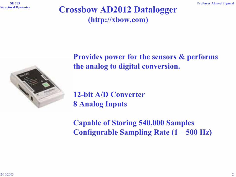
Crossbow AD2012 Datalogger(http://xbow.com)
Provides power for the sensors & performs the analog to digital conversion.
12-bit A/D Converter8 Analog Inputs
Capable of Storing 540,000 SamplesConfigurable Sampling Rate (1 – 500 Hz)
2/10/2003 3
SE 203Structural Dynamics
Professor Ahmed Elgamal
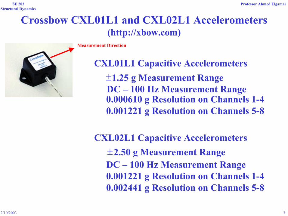
CXL01L1 Capacitive Accelerometers
Crossbow CXL01L1 and CXL02L1 Accelerometers(http://xbow.com)
1.25 g Measurement Range±
0.000610 g Resolution on Channels 1-40.001221 g Resolution on Channels 5-8
CXL02L1 Capacitive Accelerometers2.50 g Measurement Range
DC – 100 Hz Measurement Range0.001221 g Resolution on Channels 1-40.002441 g Resolution on Channels 5-8
DC – 100 Hz Measurement Range
±
Measurement Direction
2/10/2003 4
SE 203Structural Dynamics
Professor Ahmed Elgamal
Field-Testing
Using the Datalogger and accelerometers, you will need to go and record acceleration time histories at various locations on your structure.
You will need to choose these locations carefully (allowing you to capture the 1st couple of modes).
Once you have recorded your data, you will need to bring the datalogger back to the IT lab (SERF 154) and download the data.
We will then save the acceleration time histories onto a CD allowing you to perform the structural identification on your own.
2/10/2003 5
SE 203Structural Dynamics
Professor Ahmed Elgamal
Checking In and Out the Equipment
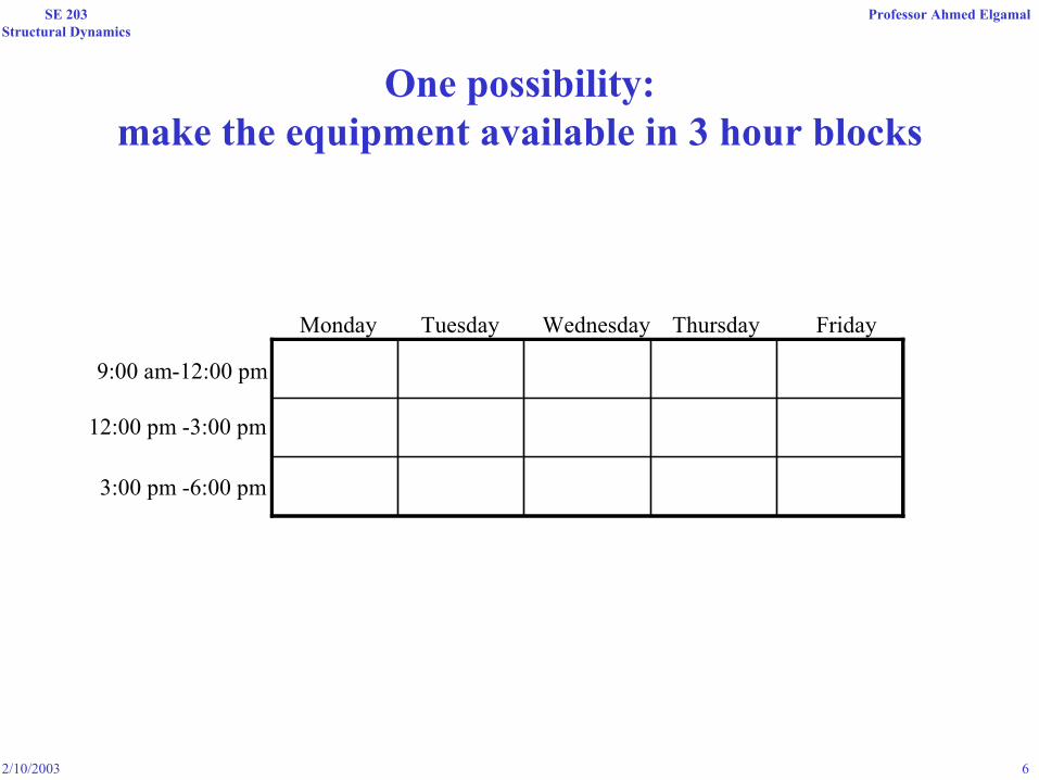
As there is only one set of testing equipment, we will set up a series of time slots. Each group will sign up for one of these and will be
expected to do their testing during this time. If more time is needed, you may either trade times with another group or try to find and
unused time slot.
Each group will be responsible for checking in the equipment before it is due back. This will allow us to service the equipment and ensure
that everything is working for the next group.
Any data left on the datalogger will be erased once it is returned.
In order to allow sufficient time for analysis, all testing must be completed by February 28. The equipment cannot be checked out
after this date!!!
2/10/2003 6
SE 203Structural Dynamics
Professor Ahmed Elgamal
Monday Tuesday Wednesday Thursday Friday
9:00 am-12:00 pm
12:00 pm -3:00 pm
3:00 pm -6:00 pm
One possibility:make the equipment available in 3 hour blocks

2/10/2003 7
SE 203Structural Dynamics
Professor Ahmed Elgamal
Crossbow AD2012 Datalogger
Crossbow CXL01L1 Accelerometer
SERF Building Rm. 154
Canon A40 PowerShot Digital Camera
2/10/2003 8
SE 203Structural Dynamics
Professor Ahmed Elgamal
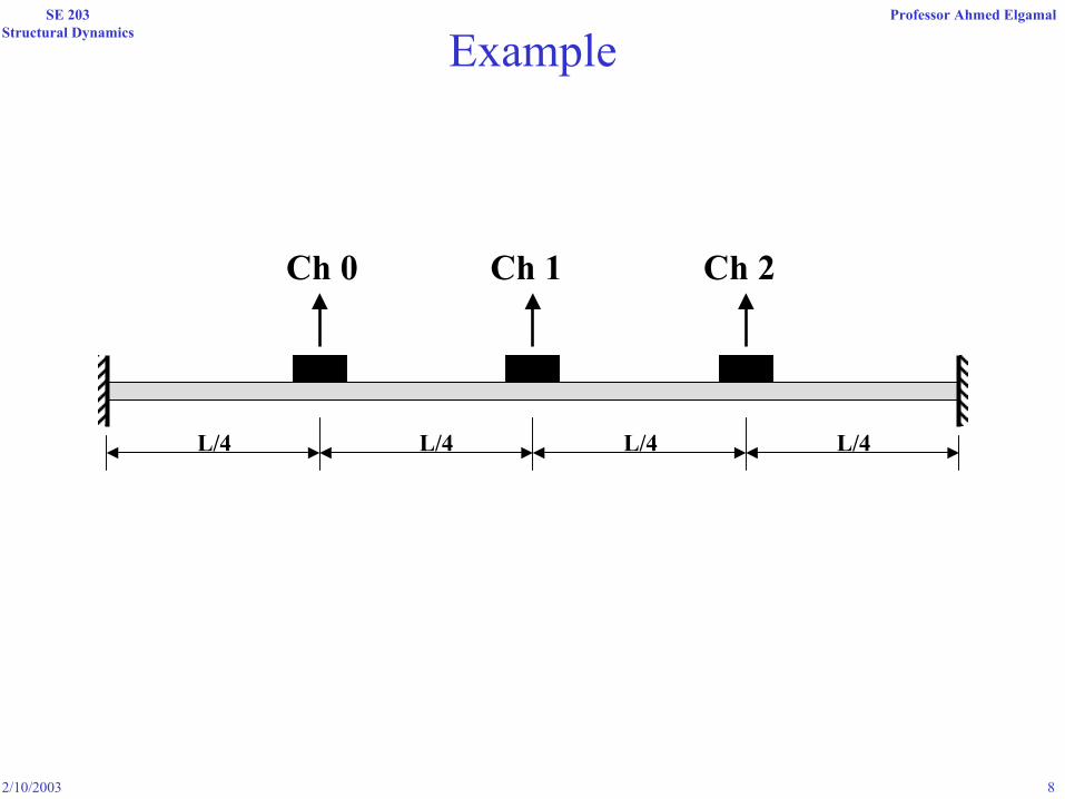
Ch 0 Ch 1 Ch 2
L/4 L/4 L/4L/4
Example

2/10/2003 9
SE 203Structural Dynamics
Professor Ahmed Elgamal
Time Domain Data

2/10/2003 10
SE 203Structural Dynamics
Professor Ahmed Elgamal
Structural Identification Tools
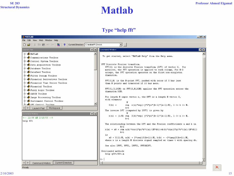
The Fast Fourier Transform (FFT) and the Power Spectrum are powerful tools for analyzing and measuring signals.
FFTs and the Power Spectrum are useful for measuring the frequency content of stationary or transient signals. FFTs produce the average frequency content of a signal over the entire time that the signal was
acquired.
∆tN1∆f⋅
=Note: the frequency resolution
where, N is in the number of samples and ∆t is the time increment.
Additional Resource: http://zone.ni.com/devzone/conceptd.nsf/webmain/C045A890751303A6862568650061EA98/$File/AN041.pdf
2/10/2003 11
SE 203Structural Dynamics
Professor Ahmed Elgamal
Power Spectrum
The units of a power spectrum are often referred to as quantity squared rms, where quantity is the unit of the time-domain signal.
The power spectrum shows power as the mean squared amplitude at each frequency line but includes no phase information.
Because the power spectrum loses phase information, you may want to use the FFT to view both the frequency and the phase
information of a signal.
2/10/2003 12
SE 203Structural Dynamics
Professor Ahmed Elgamal
Fourier Transform
The phase information the FFT yields is the phase relative to the start of the time-domain signal. For this reason, you must trigger from the same point in the signal to obtain consistent phase readings. In many cases, your concern is the relative phases between components, or the
phase difference between two signals acquired simultaneously.
The FFT returns a two-sided spectrum in complex form (real and imaginary parts), which you must scale and convert to polar form to
obtain magnitude and phase. The frequency axis is identical to that of the two-sided power spectrum. The amplitude of the FFT is related to
the number of points in the time-domain signal.

2/10/2003 13
SE 203Structural Dynamics
Professor Ahmed Elgamal
Cross Power Spectrum
Cross Power Spectrum ( )2AB N
AFFTFFT(B)(f)S∗×
=
The cross power spectrum is a useful tool for determining the phase difference between two signals.
The two-sided cross power spectrum of two time-domain signals A and B is computed as:

2/10/2003 14
SE 203Structural Dynamics
Professor Ahmed Elgamal
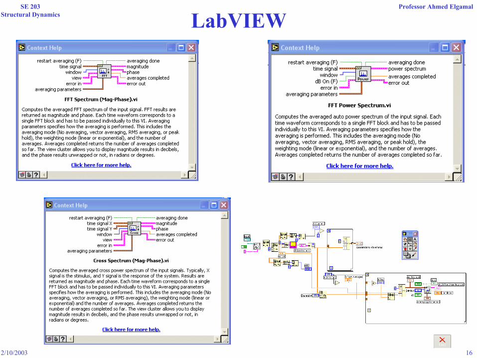
LabVIEW
Excel
Fortran
Matlab
These operations can be done in:
2/10/2003 15
SE 203Structural Dynamics
Professor Ahmed Elgamal
Matlab
Type “help fft”
2/10/2003 16
SE 203Structural Dynamics
Professor Ahmed Elgamal
LabVIEW

2/10/2003 17
SE 203Structural Dynamics
Professor Ahmed Elgamal
ExcelThis operation requires the Analysis ToolPak
2/10/2003 18
SE 203Structural Dynamics
Professor Ahmed Elgamal
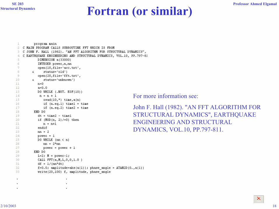
Fortran (or similar)
For more information see:
John F. Hall (1982). "AN FFT ALGORITHM FOR STRUCTURAL DYNAMICS", EARTHQUAKE ENGINEERING AND STRUCTURAL DYNAMICS, VOL.10, PP.797-811.
.
.
.
.
.
.

2/10/2003 19
SE 203Structural Dynamics
Professor Ahmed Elgamal
Example: Power Spectrum
0.0000080000
0.0000000000
0.0000010000
0.0000020000
0.0000030000
0.0000040000
0.0000050000
0.0000060000
0.0000070000
50.00.0 10.0 20.0 30.0 40.0
Ch 0
Power Spectrum

2/10/2003 20
SE 203Structural Dynamics
Professor Ahmed Elgamal
Averaging
To smooth the spectrum, we need to average the data.
This can be done by:
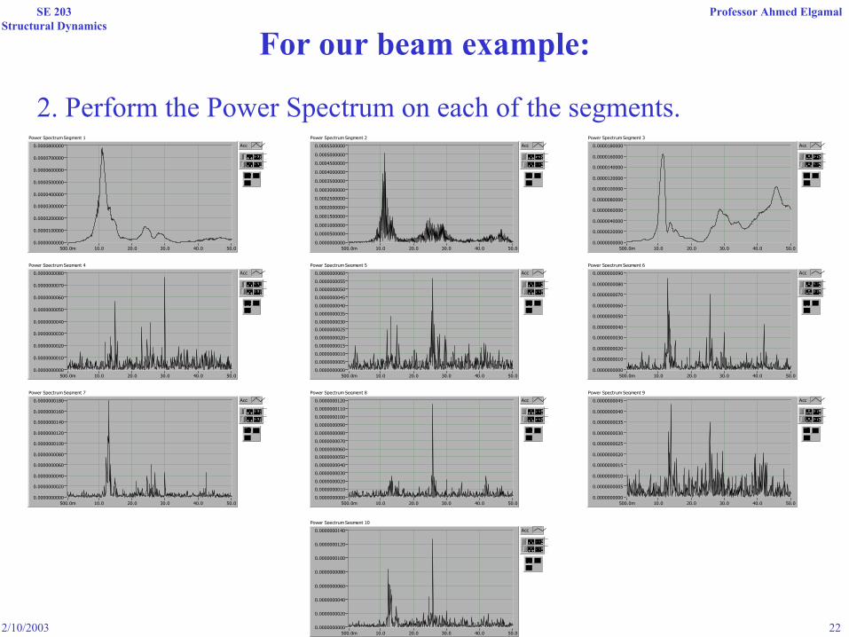
1. Splitting the time history into a number of equally sized segments.
2. Performing an FFT (or Cross Spectrum) on each of the segments.
3. Averaging each of these segments (Magnitude & Phase). Start by converting to complex form (Real and Imaginary). Then sum the two real components at each increment of frequency and then divide by the number of averages. Do the same for the imaginary. When you are done, convert back to magnitude and phase.

2/10/2003 21
SE 203Structural Dynamics
Professor Ahmed Elgamal
For our beam example:
1. Split the time history into 10 segments each 12 seconds long.1.0000000000
-1.2000000000
-1.0000000000
-0.8000000000
-0.6000000000
-0.4000000000
-0.2000000000
0.0000000000
0.2000000000
0.4000000000
0.6000000000
0.8000000000
12.00.0 2.0 4.0 6.0 8.0 10.0
Acc
Acceleration Segment 1
1.0000000000
-1.2000000000
-1.0000000000
-0.8000000000
-0.6000000000
-0.4000000000
-0.2000000000
0.0000000000
0.2000000000
0.4000000000
0.6000000000
0.8000000000
24.012.0 14.0 16.0 18.0 20.0 22.0
Acc
Acceleration Segment 2
1.0000000000
-1.0000000000
-0.8000000000
-0.6000000000
-0.4000000000
-0.2000000000
0.0000000000
0.2000000000
0.4000000000
0.6000000000
0.8000000000
36.024.0 26.0 28.0 30.0 32.0 34.0
Acc
Acceleration Segment 3
0.0035000000
-0.0030000000
-0.0025000000
-0.0020000000
-0.0015000000
-0.0010000000
-0.0005000000
0.0000000000
0.0005000000
0.0010000000
0.0015000000
0.0020000000
0.0025000000
0.0030000000
48.036.0 38.0 40.0 42.0 44.0 46.0
Acc
Acceleration Segment 4
0.0025000000
-0.0025000000
-0.0020000000
-0.0015000000
-0.0010000000
-0.0005000000
0.0000000000
0.0005000000
0.0010000000
0.0015000000
0.0020000000
60.048.0 50.0 52.0 54.0 56.0 58.0
Acc
Acceleration Segment 5
0.0025000000
-0.0025000000
-0.0020000000
-0.0015000000
-0.0010000000
-0.0005000000
0.0000000000
0.0005000000
0.0010000000
0.0015000000
0.0020000000
72.060.0 62.0 64.0 66.0 68.0 70.0
Acc
Acceleration Segment 6
0.0030000000
-0.0025000000
-0.0020000000
-0.0015000000
-0.0010000000
-0.0005000000
0.0000000000
0.0005000000
0.0010000000
0.0015000000
0.0020000000
0.0025000000
84.072.0 74.0 76.0 78.0 80.0 82.0
Acc
Acceleration Segment 7
0.0025000000
-0.0020000000
-0.0015000000
-0.0010000000
-0.0005000000
0.0000000000
0.0005000000
0.0010000000
0.0015000000
0.0020000000
96.084.0 86.0 88.0 90.0 92.0 94.0
Acc
Acceleration Segment 8
0.0025000000
-0.0025000000
-0.0020000000
-0.0015000000
-0.0010000000
-0.0005000000
0.0000000000
0.0005000000
0.0010000000
0.0015000000
0.0020000000
108.096.0 98.0 100.0 102.0 104.0 106.0
Acc
Acceleration Segment 9
0.0025000000
-0.0030000000
-0.0025000000
-0.0020000000
-0.0015000000
-0.0010000000
-0.0005000000
0.0000000000
0.0005000000
0.0010000000
0.0015000000
0.0020000000
120.0108.0 110.0 112.0 114.0 116.0 118.0
Acc
Acceleration Segment 10
2/10/2003 22
SE 203Structural Dynamics
Professor Ahmed Elgamal
For our beam example:
2. Perform the Power Spectrum on each of the segments.0.0000800000
0.0000000000
0.0000100000
0.0000200000
0.0000300000
0.0000400000
0.0000500000
0.0000600000
0.0000700000
50.0500.0m 10.0 20.0 30.0 40.0
Acc
Power Spectrum Segment 1
0.0005500000
0.0000000000
0.0000500000
0.0001000000
0.0001500000
0.0002000000
0.0002500000
0.0003000000
0.0003500000
0.0004000000
0.0004500000
0.0005000000
50.0500.0m 10.0 20.0 30.0 40.0
Acc
Power Spectrum Segment 2
0.0000180000
0.0000000000
0.0000020000
0.0000040000
0.0000060000
0.0000080000
0.0000100000
0.0000120000
0.0000140000
0.0000160000
50.0500.0m 10.0 20.0 30.0 40.0
Acc
Power Spectrum Segment 3
0.0000000080
0.0000000000
0.0000000010
0.0000000020
0.0000000030
0.0000000040
0.0000000050
0.0000000060
0.0000000070
50.0500.0m 10.0 20.0 30.0 40.0
Acc
Power Spectrum Segment 4
0.0000000060
0.0000000000
0.0000000005
0.0000000010
0.0000000015
0.0000000020
0.0000000025
0.0000000030
0.0000000035
0.0000000040
0.0000000045
0.0000000050
0.0000000055
50.0500.0m 10.0 20.0 30.0 40.0
Acc
Power Spectrum Segment 5
0.0000000090
0.0000000000
0.0000000010
0.0000000020
0.0000000030
0.0000000040
0.0000000050
0.0000000060
0.0000000070
0.0000000080
50.0500.0m 10.0 20.0 30.0 40.0
Acc
Power Spectrum Segment 6
0.0000000180
0.0000000000
0.0000000020
0.0000000040
0.0000000060
0.0000000080
0.0000000100
0.0000000120
0.0000000140
0.0000000160
50.0500.0m 10.0 20.0 30.0 40.0
Acc
Power Spectrum Segment 7
0.0000000120
0.0000000000
0.0000000010
0.0000000020
0.0000000030
0.0000000040
0.0000000050
0.0000000060
0.0000000070
0.0000000080
0.0000000090
0.0000000100
0.0000000110
50.0500.0m 10.0 20.0 30.0 40.0
Acc
Power Spectrum Segment 8
0.0000000045
0.0000000000
0.0000000005
0.0000000010
0.0000000015
0.0000000020
0.0000000025
0.0000000030
0.0000000035
0.0000000040
50.0500.0m 10.0 20.0 30.0 40.0
Acc
Power Spectrum Segment 9
0.0000000140
0.0000000000
0.0000000020
0.0000000040
0.0000000060
0.0000000080
0.0000000100
0.0000000120
50.0500.0m 10.0 20.0 30.0 40.0
Acc
Power Spectrum Segment 10

2/10/2003 23
SE 203Structural Dynamics
Professor Ahmed Elgamal
For our beam example:3. Average each of the segments
0.0000080000
0.0000000000
0.0000010000
0.0000020000
0.0000030000
0.0000040000
0.0000050000
0.0000060000
0.0000070000
50.00.0 10.0 20.0 30.0 40.0
Ch 0
Averaged Power Spectrum (1 Average)
0.0000180000
0.0000000000
0.0000020000
0.0000040000
0.0000060000
0.0000080000
0.0000100000
0.0000120000
0.0000140000
0.0000160000
50.00.0 10.0 20.0 30.0 40.0
Ch 0
Averaged Power Spectrum (2 Averages)
0.0000350000
0.0000000000
0.0000050000
0.0000100000
0.0000150000
0.0000200000
0.0000250000
0.0000300000
50.00.0 10.0 20.0 30.0 40.0
Ch 0
Averaged Power Spectrum (3 Averages)
0.0000500000
0.0000000000
0.0000050000
0.0000100000
0.0000150000
0.0000200000
0.0000250000
0.0000300000
0.0000350000
0.0000400000
0.0000450000
50.00.0 10.0 20.0 30.0 40.0
Ch 0
Averaged Power Spectrum (4 Averages)
0.0000700000
0.0000000000
0.0000100000
0.0000200000
0.0000300000
0.0000400000
0.0000500000
0.0000600000
50.00.0 10.0 20.0 30.0 40.0
Ch 0
Averaged Power Spectrum (5 Averages)0.0000900000
0.0000000000
0.0000100000
0.0000200000
0.0000300000
0.0000400000
0.0000500000
0.0000600000
0.0000700000
0.0000800000
50.00.0 10.0 20.0 30.0 40.0
Ch 0
Averaged Power Spectrum (6 Averages)
0.0000650000
0.0000000000
0.0000050000
0.0000100000
0.0000150000
0.0000200000
0.0000250000
0.0000300000
0.0000350000
0.0000400000
0.0000450000
0.0000500000
0.0000550000
0.0000600000
50.00.0 10.0 20.0 30.0 40.0
Ch 0
Averaged Power Spectrum (7 Averages)
0.0000800000
0.0000000000
0.0000100000
0.0000200000
0.0000300000
0.0000400000
0.0000500000
0.0000600000
0.0000700000
50.00.0 10.0 20.0 30.0 40.0
Ch 0
Averaged Power Spectrum (8 Averages)
0.0000350000
0.0000000000
0.0000050000
0.0000100000
0.0000150000
0.0000200000
0.0000250000
0.0000300000
50.00.0 10.0 20.0 30.0 40.0
Ch 0
Averaged Power Spectrum (9 Averages)
0.0000350000
0.0000000000
0.0000050000
0.0000100000
0.0000150000
0.0000200000
0.0000250000
0.0000300000
50.00.0 10.0 20.0 30.0 40.0
Ch 0
Averaged Power Spectrum (10 Averages)
Do the Same for the Phase Angle
2/10/2003 24
SE 203Structural Dynamics
Professor Ahmed Elgamal
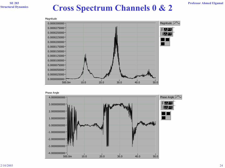
Cross Spectrum Channels 0 & 20.0000300000
0.0000000000
0.0000025000
0.0000050000
0.0000075000
0.0000100000
0.0000125000
0.0000150000
0.0000175000
0.0000200000
0.0000225000
0.0000250000
0.0000275000
50.0500.0m 10.0 20.0 30.0 40.0
Magnitude
Magnitude
4.0000000000
-4.0000000000
-3.0000000000
-2.0000000000
-1.0000000000
0.0000000000
1.0000000000
2.0000000000
3.0000000000
50.0500.0m 10.0 20.0 30.0 40.0
Phase Angle
Phase Angle

2/10/2003 25
SE 203Structural Dynamics
Professor Ahmed Elgamal
Cross Spectrum Channels 0 & 10.0000300000
0.0000000000
0.0000025000
0.0000050000
0.0000075000
0.0000100000
0.0000125000
0.0000150000
0.0000175000
0.0000200000
0.0000225000
0.0000250000
0.0000275000
50.0500.0m 10.0 20.0 30.0 40.0
Magnitude
Magnitude
4.0000000000
-4.0000000000
-3.0000000000
-2.0000000000
-1.0000000000
0.0000000000
1.0000000000
2.0000000000
3.0000000000
50.0500.0m 10.0 20.0 30.0 40.0
Phase Angle
Phase Angle

2/10/2003 26
SE 203Structural Dynamics
Professor Ahmed Elgamal
Construct the Mode Shapes
1. From the Magnitude, determine the relative amplitude.
2. From the Phase Angle, determine the sign.
For our example, let’s start with the 1st mode
2/10/2003 27
SE 203Structural Dynamics
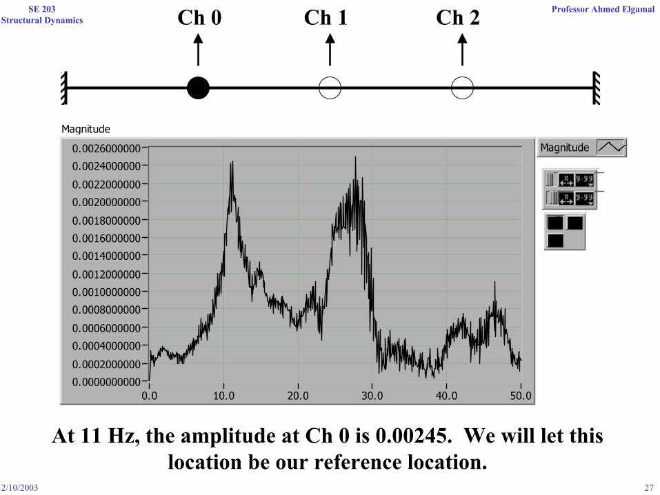
Professor Ahmed ElgamalCh 0 Ch 1 Ch 2
0.0026000000
0.0000000000
0.0002000000
0.0004000000
0.0006000000
0.0008000000
0.0010000000
0.0012000000
0.0014000000
0.0016000000
0.0018000000
0.0020000000
0.0022000000
0.0024000000
50.00.0 10.0 20.0 30.0 40.0
Magnitude
Magnitude
At 11 Hz, the amplitude at Ch 0 is 0.00245. We will let this location be our reference location.

2/10/2003 28
SE 203Structural Dynamics
Professor Ahmed ElgamalCh 0 Ch 1 Ch 2
At 11 Hz, the amplitude at Ch 1 is 0.00382.
2/10/2003 29
SE 203Structural Dynamics
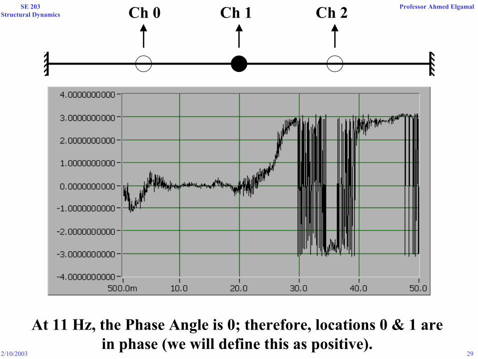
Professor Ahmed ElgamalCh 0 Ch 1 Ch 2
At 11 Hz, the Phase Angle is 0; therefore, locations 0 & 1 are in phase (we will define this as positive).
2/10/2003 30
SE 203Structural Dynamics
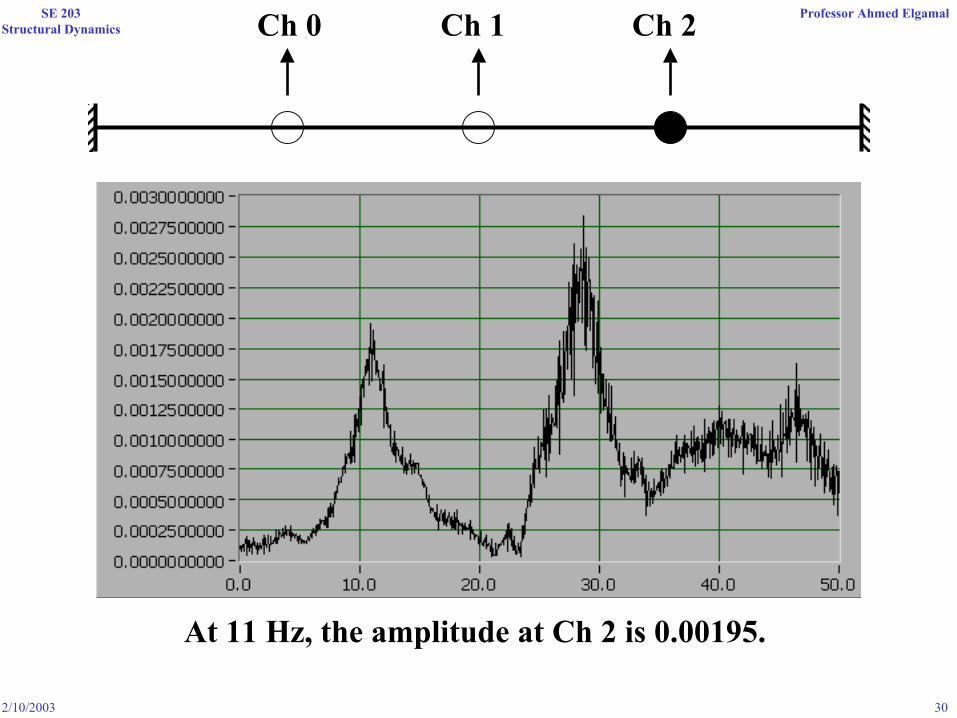
Professor Ahmed ElgamalCh 0 Ch 1 Ch 2
At 11 Hz, the amplitude at Ch 2 is 0.00195.
2/10/2003 31
SE 203Structural Dynamics
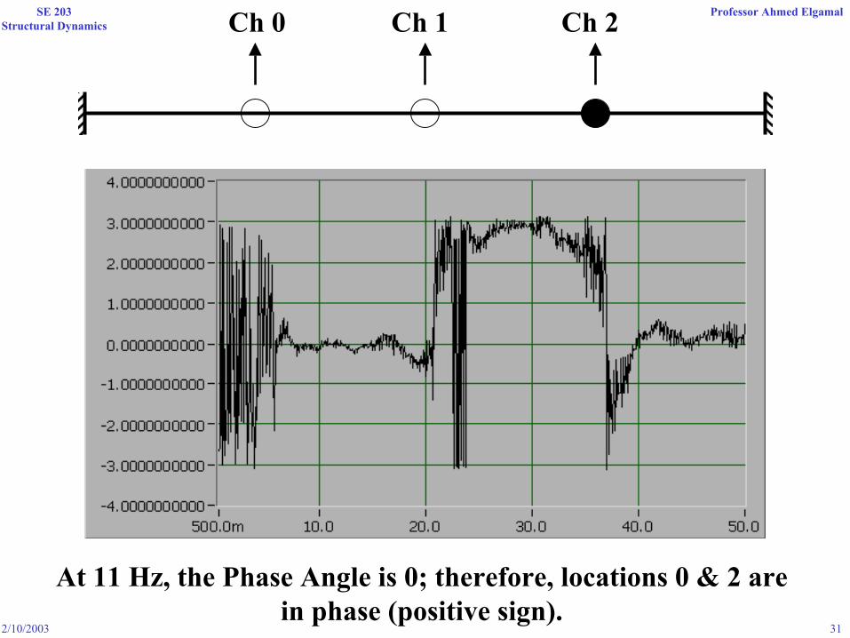
Professor Ahmed ElgamalCh 0 Ch 1 Ch 2
At 11 Hz, the Phase Angle is 0; therefore, locations 0 & 2 are in phase (positive sign).

2/10/2003 32
SE 203Structural Dynamics
Professor Ahmed Elgamal
0.002450.00382
0.00195
First Mode Shape
2/10/2003 33
SE 203Structural Dynamics
Professor Ahmed Elgamal
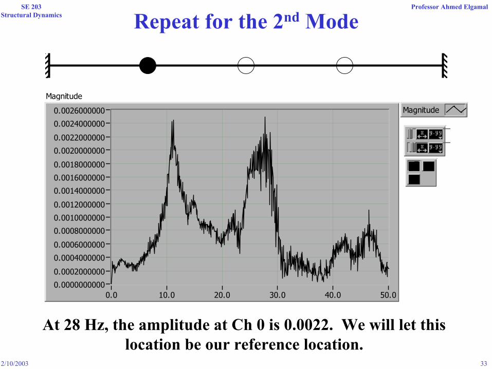
Repeat for the 2nd Mode
0.0026000000
0.0000000000
0.0002000000
0.0004000000
0.0006000000
0.0008000000
0.0010000000
0.0012000000
0.0014000000
0.0016000000
0.0018000000
0.0020000000
0.0022000000
0.0024000000
50.00.0 10.0 20.0 30.0 40.0
Magnitude
Magnitude
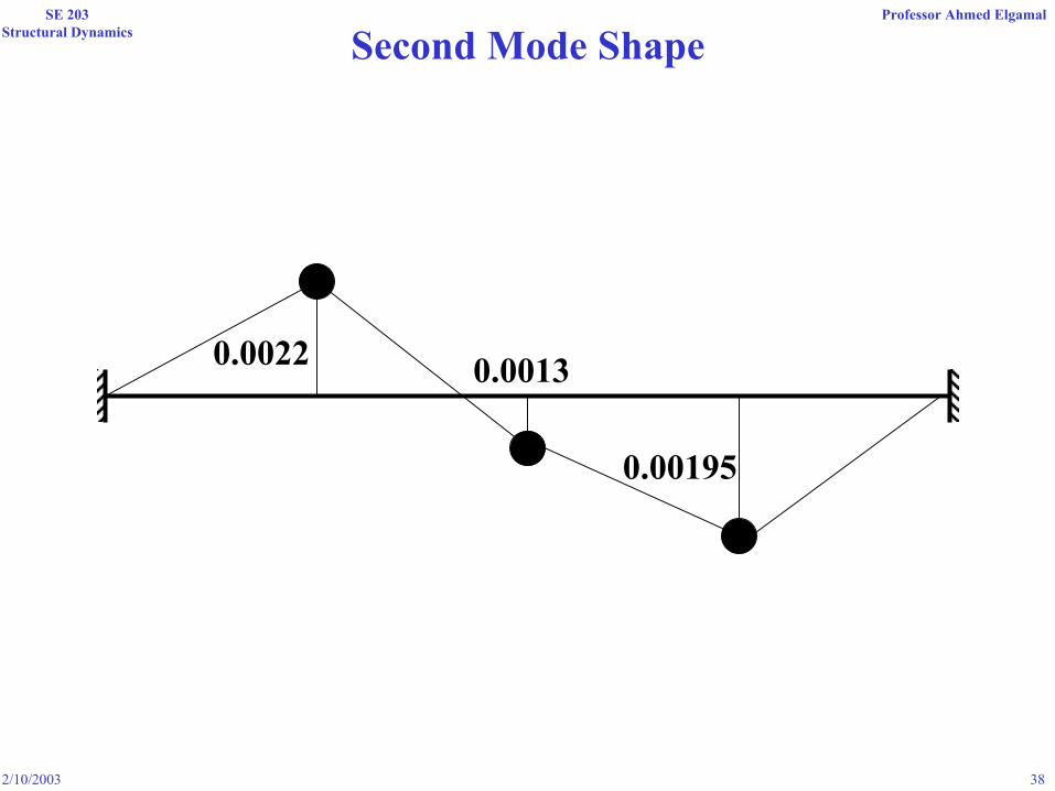
At 28 Hz, the amplitude at Ch 0 is 0.0022. We will let this location be our reference location.
2/10/2003 34
SE 203Structural Dynamics
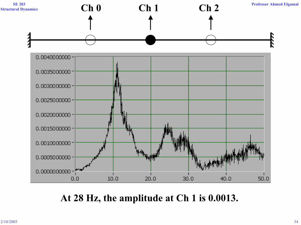
Professor Ahmed ElgamalCh 0 Ch 1 Ch 2
At 28 Hz, the amplitude at Ch 1 is 0.0013.
2/10/2003 35
SE 203Structural Dynamics
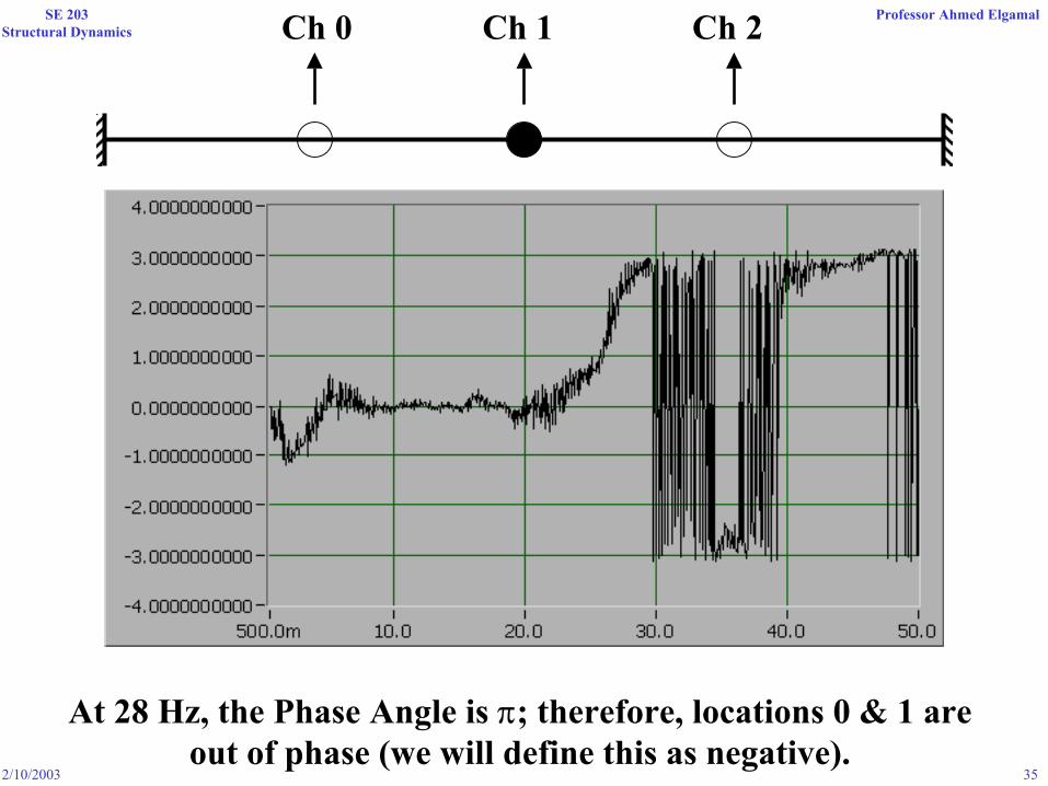
Professor Ahmed ElgamalCh 0 Ch 1 Ch 2
At 28 Hz, the Phase Angle is π; therefore, locations 0 & 1 are out of phase (we will define this as negative).

2/10/2003 36
SE 203Structural Dynamics
Professor Ahmed ElgamalCh 0 Ch 1 Ch 2
At 28 Hz, the amplitude at Ch 2 is 0.0026.

2/10/2003 37
SE 203Structural Dynamics
Professor Ahmed ElgamalCh 0 Ch 1 Ch 2
At 28 Hz, the Phase Angle is π; therefore, locations 0 & 2 are out of phase (negative sign).
2/10/2003 38
SE 203Structural Dynamics
Professor Ahmed Elgamal
0.0022 0.0013
0.00195
Second Mode Shape
2/10/2003 39
SE 203Structural Dynamics
Professor Ahmed Elgamal
Hints
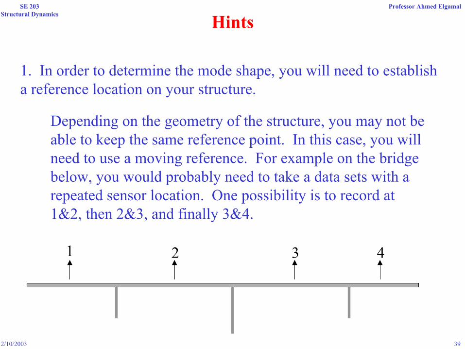
1. In order to determine the mode shape, you will need to establish a reference location on your structure.
Depending on the geometry of the structure, you may not be able to keep the same reference point. In this case, you will need to use a moving reference. For example on the bridge below, you would probably need to take a data sets with a repeated sensor location. One possibility is to record at 1&2, then 2&3, and finally 3&4.
1 2 3 4
2/10/2003 40
SE 203Structural Dynamics
Professor Ahmed Elgamal
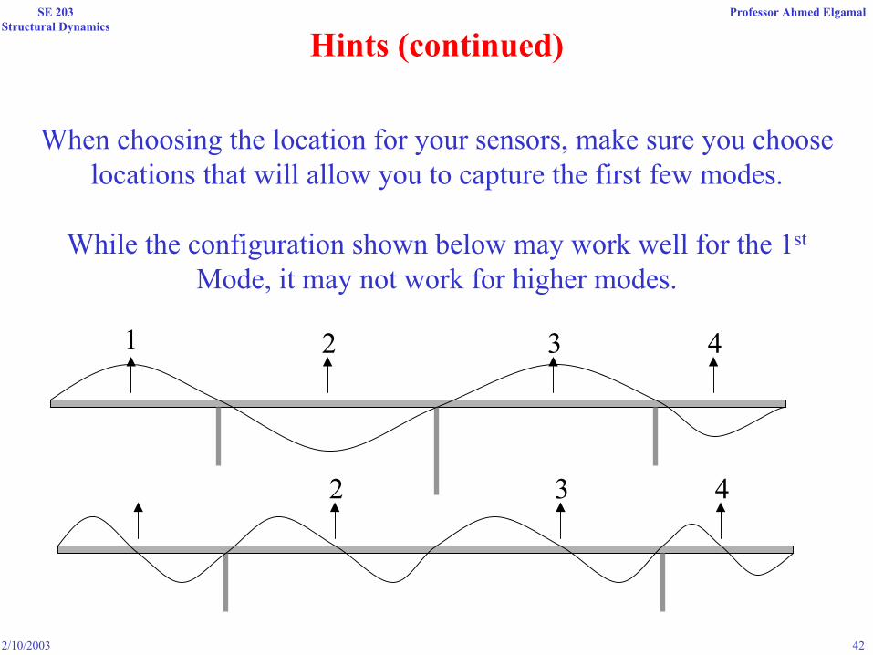
Hints (continued)
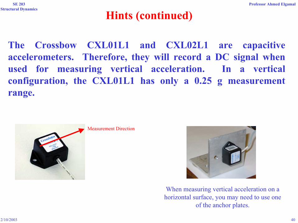
The Crossbow CXL01L1 and CXL02L1 are capacitive accelerometers. Therefore, they will record a DC signal when used for measuring vertical acceleration. In a vertical configuration, the CXL01L1 has only a 0.25 g measurement range.
Measurement Direction
When measuring vertical acceleration on a horizontal surface, you may need to use one
of the anchor plates.
2/10/2003 41
SE 203Structural Dynamics
Professor Ahmed Elgamal
Hints (continued)
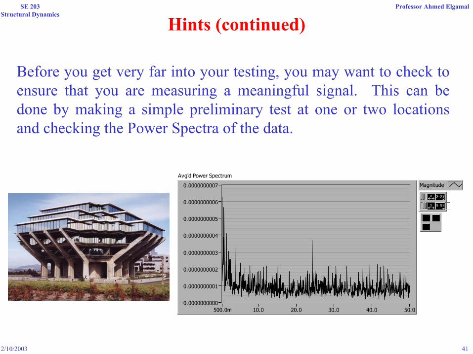
Before you get very far into your testing, you may want to check to ensure that you are measuring a meaningful signal. This can be done by making a simple preliminary test at one or two locationsand checking the Power Spectra of the data.
0.0000000007
0.0000000000
0.0000000001
0.0000000002
0.0000000003
0.0000000004
0.0000000005
0.0000000006
50.0500.0m 10.0 20.0 30.0 40.0
Magnitude
Avg'd Power Spectrum
2/10/2003 42
SE 203Structural Dynamics
Professor Ahmed Elgamal
Hints (continued)
1 2 3 4
When choosing the location for your sensors, make sure you choose locations that will allow you to capture the first few modes.
While the configuration shown below may work well for the 1st
Mode, it may not work for higher modes.
2 3 4

2/10/2003 43
SE 203Structural Dynamics
Professor Ahmed Elgamal
Running theCrossbow DataReady Software
2/10/2003 44
SE 203Structural Dynamics
Professor Ahmed Elgamal
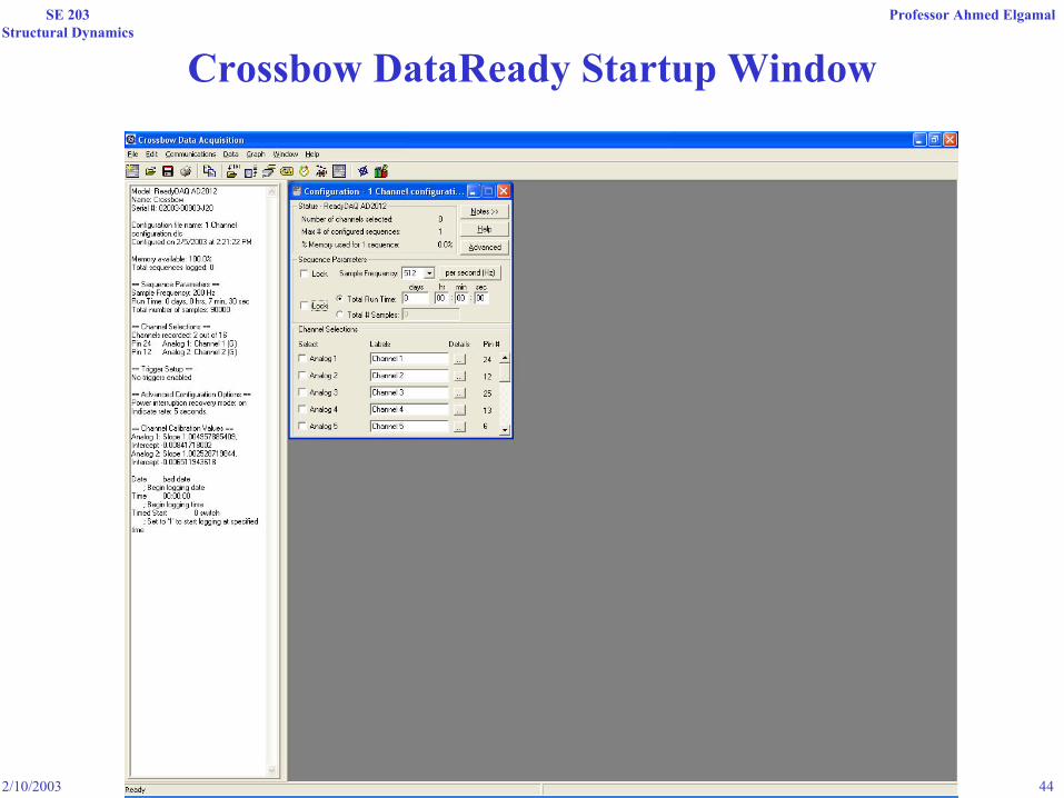
Crossbow DataReady Startup Window

2/10/2003 45
SE 203Structural Dynamics
Professor Ahmed Elgamal
Datalogger Status

2/10/2003 46
SE 203Structural Dynamics
Professor Ahmed Elgamal
Current Datalogger Configuration
2/10/2003 47
SE 203Structural Dynamics
Professor Ahmed Elgamal
Configuring the Datalogger
Select Active ChannelsConfigure each of the channels
Set Sampling Frequency
Set Total Run Time
2/10/2003 48
SE 203Structural Dynamics
Professor Ahmed Elgamal
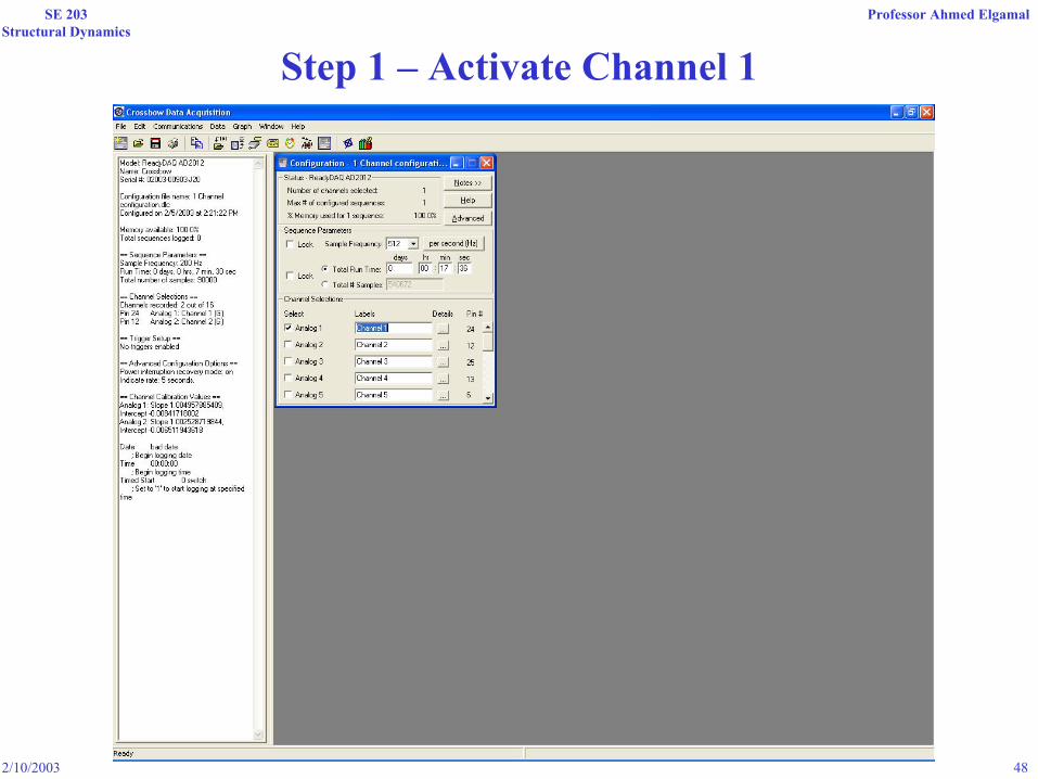
Step 1 – Activate Channel 1
2/10/2003 49
SE 203Structural Dynamics
Professor Ahmed Elgamal
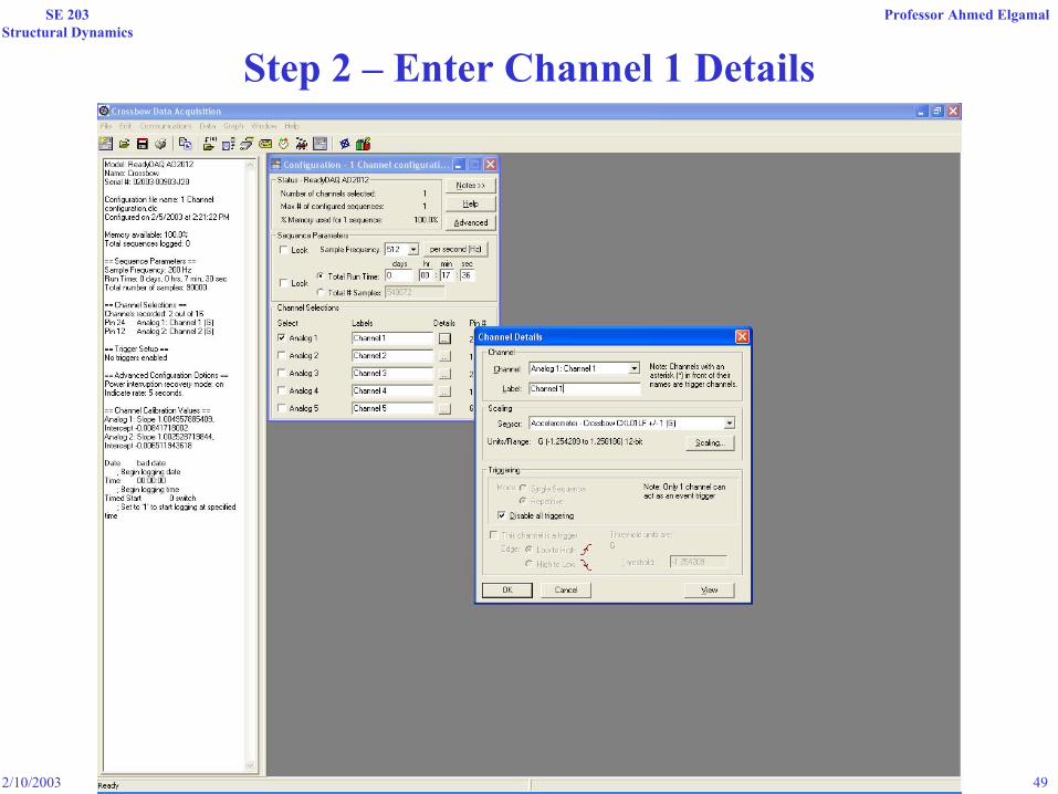
Step 2 – Enter Channel 1 Details
2/10/2003 50
SE 203Structural Dynamics
Professor Ahmed Elgamal
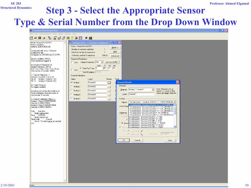
Step 3 - Select the Appropriate Sensor Type & Serial Number from the Drop Down Window
2/10/2003 51
SE 203Structural Dynamics
Professor Ahmed Elgamal
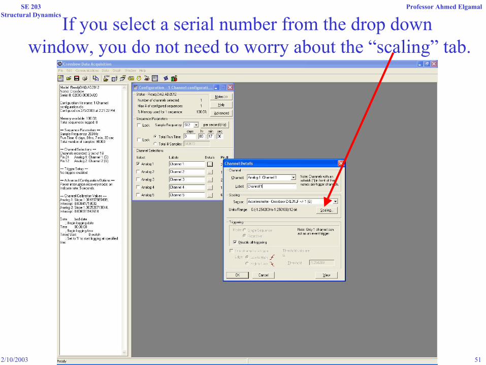
If you select a serial number from the drop downwindow, you do not need to worry about the “scaling” tab.
2/10/2003 52
SE 203Structural Dynamics
Professor Ahmed Elgamal
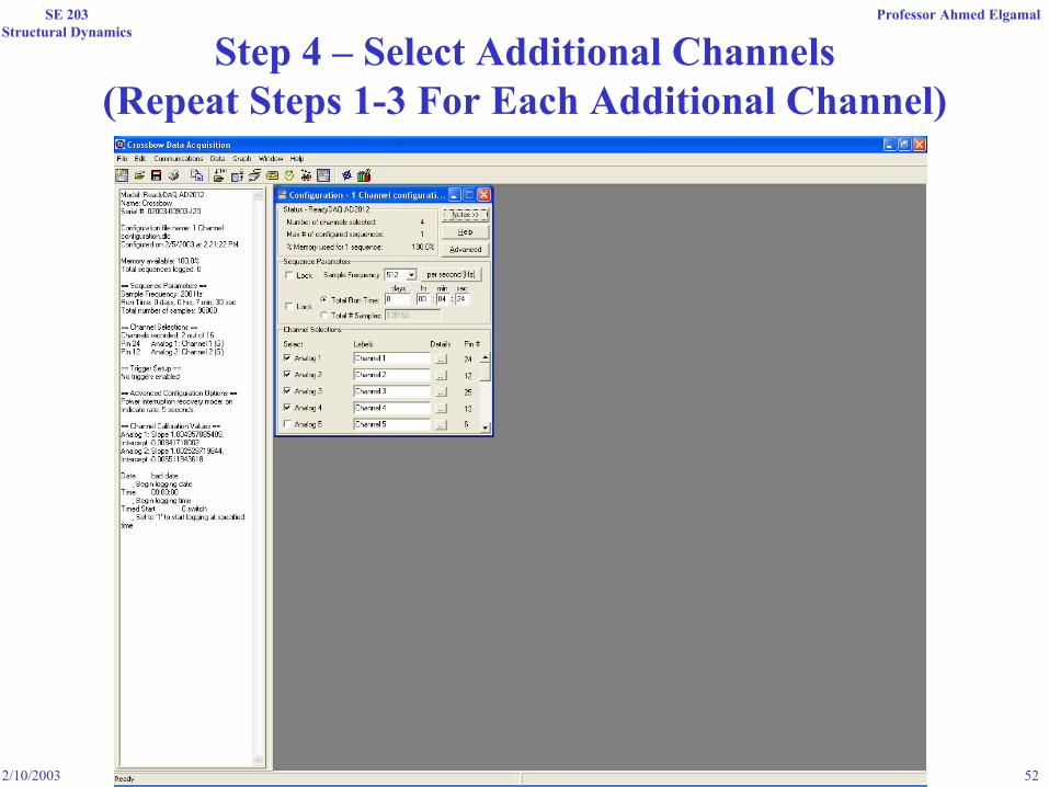
Step 4 – Select Additional Channels (Repeat Steps 1-3 For Each Additional Channel)

2/10/2003 53
SE 203Structural Dynamics
Professor Ahmed Elgamal
Step 5 – Set Desired “Sample Frequency” In the Drop Down Window

2/10/2003 54
SE 203Structural Dynamics
Professor Ahmed Elgamal
Step 6 – Enter “Total Run Time”
The “Total Run Time” is limited by the
maximum number of
samples that the data logger
can store.
2/10/2003 55
SE 203Structural Dynamics
Professor Ahmed Elgamal
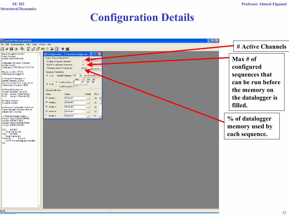
Configuration Details
# Active Channels
Max # of configured sequences that can be run before the memory on the datalogger is filled.
% of dataloggermemory used by each sequence.
2/10/2003 56
SE 203Structural Dynamics
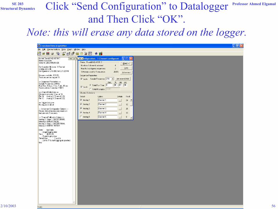
Professor Ahmed ElgamalClick “Send Configuration” to Datalogger and Then Click “OK”.
Note: this will erase any data stored on the logger.
2/10/2003 57
SE 203Structural Dynamics
Professor Ahmed Elgamal
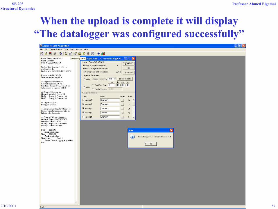
When the upload is complete it will display“The datalogger was configured successfully”
2/10/2003 58
SE 203Structural Dynamics
Professor Ahmed Elgamal
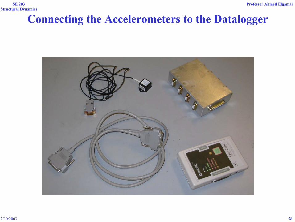
Connecting the Accelerometers to the Datalogger

2/10/2003 59
SE 203Structural Dynamics
Professor Ahmed Elgamal
Plug the accelerometer into the desired port on the junction box.
Ports on the junction box are numbered
2/10/2003 60
SE 203Structural Dynamics
Professor Ahmed Elgamal
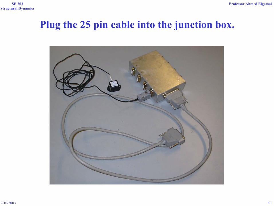
Plug the 25 pin cable into the junction box.
2/10/2003 61
SE 203Structural Dynamics
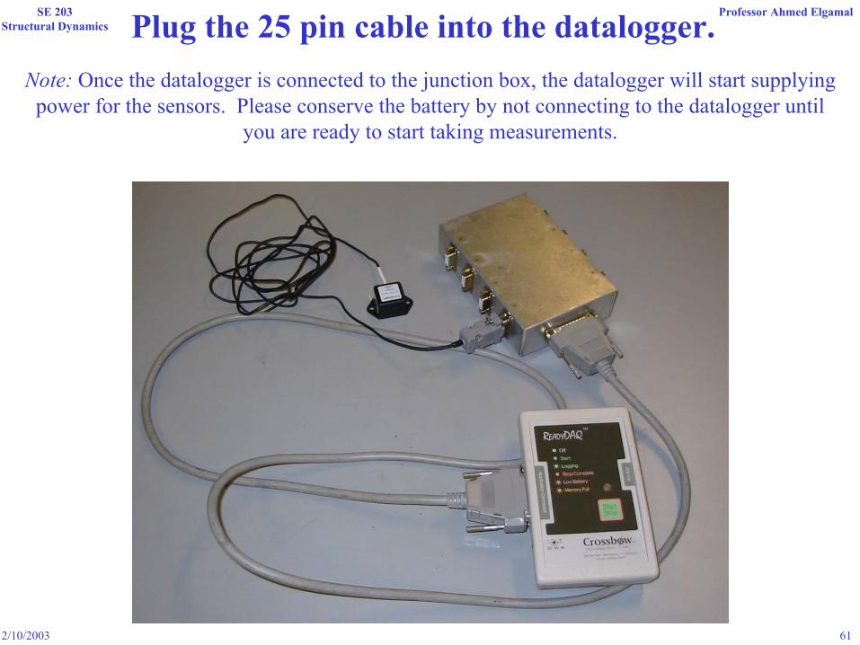
Professor Ahmed ElgamalPlug the 25 pin cable into the datalogger.Note: Once the datalogger is connected to the junction box, the datalogger will start supplying
power for the sensors. Please conserve the battery by not connecting to the datalogger until you are ready to start taking measurements.
2/10/2003 62
SE 203Structural Dynamics
Professor Ahmed Elgamal
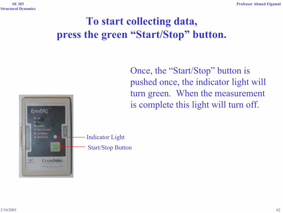
To start collecting data, press the green “Start/Stop” button.
Indicator Light
Start/Stop Button
Once, the “Start/Stop” button is pushed once, the indicator light will turn green. When the measurement is complete this light will turn off.
2/10/2003 63
SE 203Structural Dynamics
Professor Ahmed Elgamal
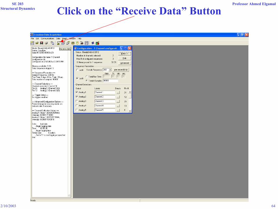
Uploading Recorded Data
1. Connect the datalogger to a PC using the RS-232 cable
2. Run the Crossbow DataReady Software
2/10/2003 64
SE 203Structural Dynamics
Professor Ahmed Elgamal
Click on the “Receive Data” Button

2/10/2003 65
SE 203Structural Dynamics
Professor Ahmed Elgamal
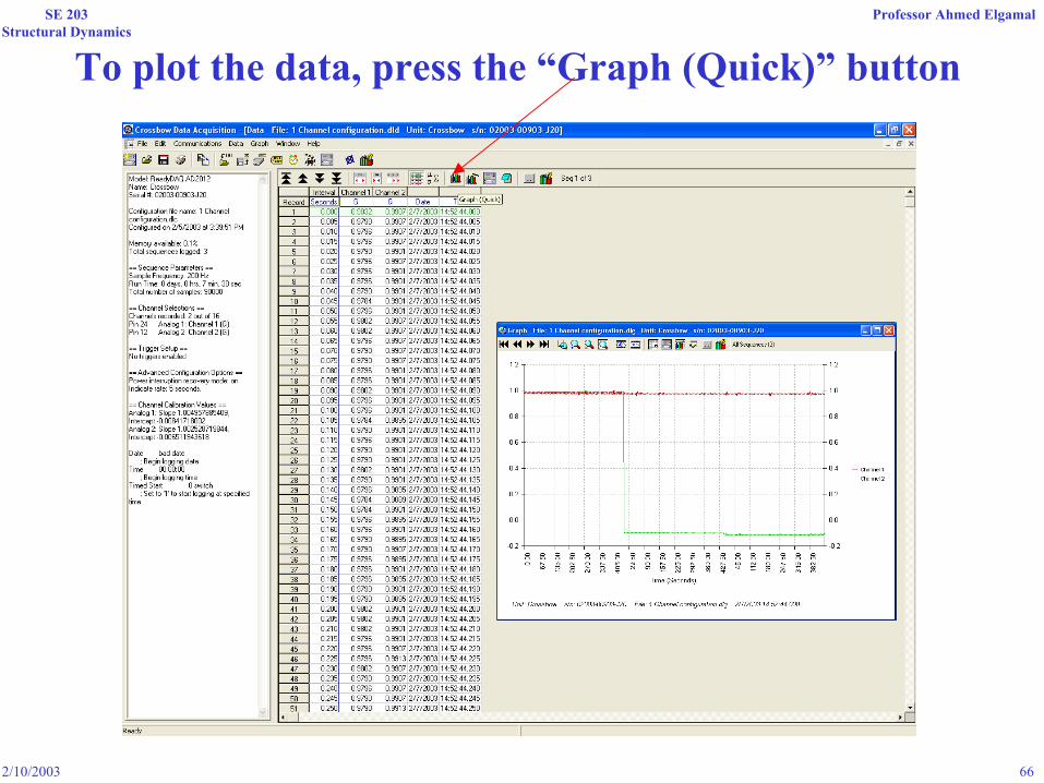
Recorded Data
2/10/2003 66
SE 203Structural Dynamics
Professor Ahmed Elgamal
To plot the data, press the “Graph (Quick)” button
2/10/2003 67
SE 203Structural Dynamics
Professor Ahmed Elgamal
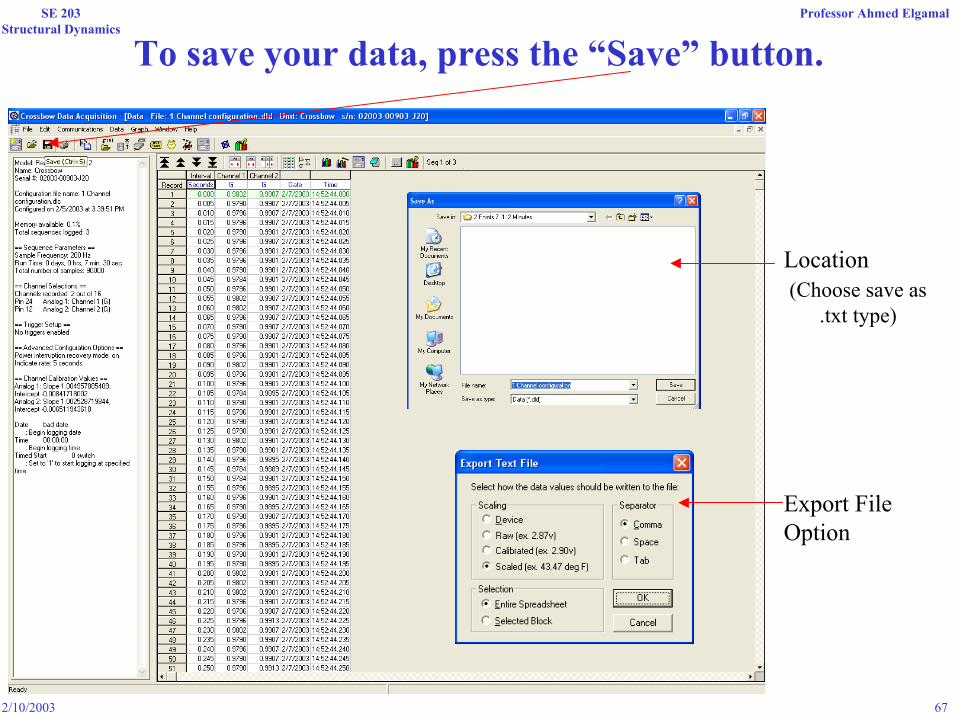
To save your data, press the “Save” button.
Location(Choose save as
.txt type)
Export File Option


