SEA WATER CONVERSION LABORATORY UNIVERSITY OF CALIFORNIA BERKELEY, CALIFORNIA FILE OPY "Study of Permeability Characteristics of Membranes" Combined Quarterly Reports Nos. 15 and 16 January 15, 1972 K. S. Spiegler, Principal Investigator R. J. Moore J. Leibovitz (part-time) R. M. Messalem (part-time) Contract No. 952109 Jet Propulsion Laboratory Pasadena, California . https://ntrs.nasa.gov/search.jsp?R=19720015450 2018-06-13T10:57:28+00:00Z
Transcript
SEA WATER CONVERSION LABORATORY
UNIVERSITY OF CALIFORNIA
BERKELEY, CALIFORNIA FILEOPY
"Study of Permeability Characteristics of Membranes"
Combined Quarterly Reports Nos. 15 and 16
January 15, 1972
K. S. Spiegler, Principal InvestigatorR. J. MooreJ. Leibovitz (part-time)R. M. Messalem (part-time)
Contract No. 952109Jet Propulsion LaboratoryPasadena, California .
"Study of Permeability Characteristics of Membranes"
Combined Quarterly Reports Nos. 15 and 16
January 15, 1972
K. S. Spiegler, Principal InvestigatorR. J. MooreJ. Leibovitz (part-time)R. M. Messalem (part-time)
Contract No. 952109Jet Propulsion LaboratoryPasadena, California
This work was performed for the Jet PropulsionLaboratory, California Institute of Technology,as sponsored by the National Aeronautics andSpace Administration under Contract NAS 7-100.
"This report contains information prepared by the University ofCalifornia, Sea Water Conversion Laboratory, Berkeley, under JPLsubcontract. Its content is not necessarily endorsed by the JetPropulsion Laboratory, California Institute of Technology, or theNational Aeronautics and Space Administration."
-TABLE.-OF CONTENTS-
Abstract, Conclusions and Recommendations 1
List of Symbols 5
Theory 7
The Duncan Transformation . 11
The Michaeli-Kedem Transformation . 19
Experimental Results 21
Method for Calculation of the L-Conductance Coefficients for theM-K Transport Equations . . . . . 25
Conclusions 37
Appendix . 42
A. 1. Relation of electrical potential differnnce, A<f>,across the membrane, to potential difference, A<j>_,between two Ag/AgCl electrodes T . . 42
A. 2. Calculation of M-K Conductivity Coefficients, L . . . 47
References 55
IV
ABSTRACT. CONCLUSIONS AND RECOMMENDATIONS
The purpose of combining two Quarterly Progress Reports under one
cover is twofold; first,the breadth of the topic treated here (viz.
bridging the gap between theory and experiment) is such that the task
was not completed at the end of the first quarter, and breaking the
results into two parts would only have caused unnecessary detouring of
the readers' effort; second, the degree of work intensity was less than
before since some staff was on summer vacation during the first quarter,
while a portion of the second quarter was in the period of the no-cost
extension of this contract, when one of the investigators (Mr. Messalem)
had left for another appointment. It is of interest that in spite of
these factors, the progress achieved in the last two quarters seems to
us of decisive importance.
A method of evaluation of the transport experiments was'worked out
which is based entirely on conservative fluxes, i.e. fluxes of quantities
which do not vary across the membrane in the steady state (the "volume
flux" and "separation flux" which have been used frequently in the past
by other investigators are not conservative). Using this procedure the
conductance coefficients for the systemi * i0.05 N NaCl C-103 cation-exchange membrane 0.1 N NaCl
were calculated. In these calculations two reciprocity relations (one
relating to salt flow - water flow coupling in osmosis and hyperfiltra-
tion L = L , the other relating membrane potential to cation transferenceo W Wo
number L = L ) were assumed to be satisfied; the third (relating streamingSc 6 J
potential to electrQQsmpsjs, L .. = .L..J was proven to hold, with.in .6 per-.. ._C W We
cent, at least up to a pressure difference of one atmosphere. In the
future it should be possible to obtain sufficiently accurate membrane
potential measurements to determine the range of validity of the reci-
procity relation L = L . We do not expect to be able to verify theoc "o
reciprocity relation LSW = LWS in our apparatus, since the pressures
necessary to determine the hyperfiltration coefficient, L , with reasonable*
accuracy are higher than our apparatus can support.
The calculation of the conductance coefficients, L, which characterize
the transport properties of the membrane, was performed with the experi-
mental data available from recent and earlier experiments. Not all of
these data were of the high accuracy which we can now achieve; moreover
some of the data came from experiments in which the membrane was in con-
tact with 0.1 N NaCl solutions on both sides, rather than 0.1 N on one
and 0.05 N on the other; but several importants points emerge from con-,
sideration of the calculated L-values (Table 4) and the methods used to
calculate these values; viz. (a) The coefficients related to a larger ex-
tent to water, w, than to salt, s, are larger (Lgw» Les; LWW » LWS; LSW » LSS;
subscript e stands for the electric current). This is probably due to the
much higher concentration of water than of salt in the ion-exchange membrane,
for the coefficients L-. increase in general with increasing c.. This propertyI j jof the set of L-coefficients thus probably reflects the exclusion of salt
from the ion-exchange membrane ("Donnan effect").
This limitation was known since the principal investigator's early high-pressure hyperfiltration experiments performed in steel vessels (1). The
— advantages-of--a-pl as tic -cell -for- the-concent-ration-el amp-apparatus -seemedso large, however, that it was decided at the start of this research toforego the determination of the validity range of the reciprocity relationLws = Lsw> tne other two reciprocity relationships can be checked in ourconcentration-clamp apparatus.
(b) The numerical calculations in section A. 2. of the Appendix show the
large dependence of all L-coefficients on the membrane conductance. In
fact, membrane conductance emerges as the most decisive transport charac-
teristic, thus justifying a posteriori the time-honored decision of battery
technologists to use conductance measurements as primary screening tests
for separator materials. The implication of this conclusion for future
experiments is the emphasis on refinements of .the technique of membrane
conductance measurements. A more elaborate and more accurate technique
than the one used in the past is being developed. It uses the existing
apparatus described in Progress Report No. 12. Apparatus and procedure
were modified to yield much more accurate measurements of the distances
of the electrodes from the membrane, (c) Consideration of the numerical
values of all terms in the calculation of the conductance parameter, L ,5
which relates the rate of electrolyte diffusion through the membrane to
the "electrolyte diffusion force", -Ay , (determined by the concentration
gradient of the electrolyte) leads one to the conclusion that osmosis +-»•
dialysis with shorted electrodes (rather than with unconnected electrodes)
should be tried, in an attempt to improve the accuracy of this determination.
Also it would be worthwhile to investigate under what conditions, if any,
the planned,'simultaneous application of several independent forces improves
the accuracy of the determination of the conductance coefficients, L.
Finally, the methods developed here for calculating a set
of L-coefficients from specified transport measurements lead to the unequi-
vocal characterization of any system of the type: solution | membrane | solution
provided only that these specified measurements can be performed with
sufficient accuracy. The "concentration-clamp" apparatus developed in
this project represents a large step towards the attainment of this experi-
mental aim.
In the future we propose to (A) measure those transport coefficients
(e.g. electrical conductance) for the system
0.05 N NaCl C-103 0.1 N NaCl
which we had previously measured only for the system
0.1 N NaCl C-103 | 0.1 N NaCl,
(B) use the method described in this report for systematic studies of
other solution-membrane systems and (C) investigate the points mentioned
under (c) above.
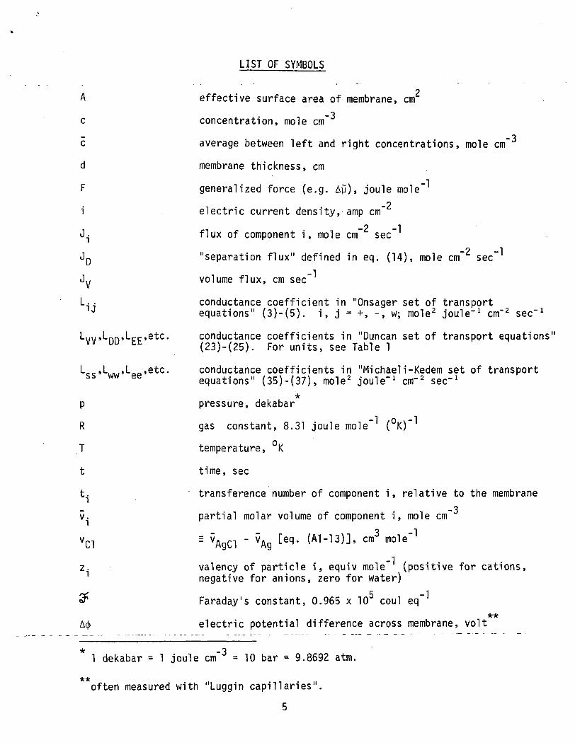
LIST OF SYMBOLS
A effective surface area of membrane, cm
c concentration, mole cm
c average between left and right concentrations, mole cm
d membrane thickness, cm
F generalized force (e.g. AM), joule mole"2
i electric current density, amp cm-2 -1J.j flux of component i, mole cm sec
o iJp "separation flux" defined in eq. (14), mole cm sec
Jy volume flux, cm sec"
L. . conductance coefficient in "Onsager set of transportJ equations" (3)-(5). i, j = +, -, w; mole2 joule"1 cm"2 sec"1
L,n;,Lnn,Lrr,etc. conductance coefficients in "Duncan set of transport equations"vv uu Lt (23)-(25). For units, see Table 1
L ,L ,L ,etc. conductance coefficients in "Michaeli-Kedem set of transport55 *"* ee equations" (35)-(37), mole2 joule"1 cnr2 sec"1
*p pressure, dekabar
R gas constant, 8.31 joule mole" (°K)"
T temperature, °K
t time, sec
t. transference number of component i, relative to the membrane-3v. partial molar volume of component i, mole cm
vcl = vAgC1 - vAg [eq. (Al-13)], cm3 mole"
z. valency of particle i, equiv mole" (positive for cations,1 negative for anions, zero for water)
f^ r _i
9" Faraday's constant, 0.965 x 10 coul eq"
**A<J> electric potential difference across membrane, volt
* 1 dekabar = 1 joule cm"3 = 10 bar = 9.8692 atm.
often measured with "Luggin capillaries".
K
P
Subscripts'
potential difference between two Ag/AgCl (anion-reversible)electrodes in solutions adjacent to membrane, volt
conductivity, ohm" cm
resistivity, ohm cm
total potential of component i [eq. (26)], joule mole-1
chemical potential of component i (includes pressure-volumeterm), joule mole"1
concentration-dependent part of chemical potential ofcomponent i, joule mole'1
w
s
cation
anion (Cl~ in this report)
water
electrolyte (NaCl in this report). Theequations refer to an electrolyte composed of a cation ofvalency +1 and an anion of valency -1 ("1-1" electrolyte)
Sign Conventions
(1) Positive direction is from left to right. (2) Fluxes from leftto right are counted positive. (3) The operator, A, for finite differencesrefers to the value on the right (double primes) minus the value on the left(single primes), as does conventionally the differential operator, d.
Driving forces are of the general form (-dy/dz). Thus positive valuesof the driving force, (-djj/dz) > 0, lead to positive fluxes. For example,Ohm's law is
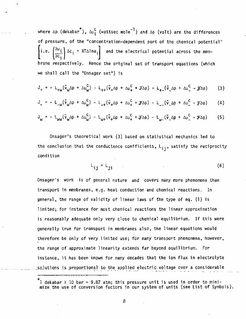
Onsager's theoretical work (3) based on statistical mechanics led to
the conclusion that the conductance coefficients, L.., satisfy the reciprocity' J
condition
Lij = Lji (6)
Onsager's work is of general nature and covers many more phenomena than
transport in membranes, e.g. heat conduction and chemical reactions. In
general, the range of validity of linear laws of the type of eq. (1) is
limited; for instance for most chemical reactions the linear approximation
is reasonably adequate only very close to chemical equilibrium. If this were
generally true for transport in membranes also, the linear equations would
therefore be only of very limited use; for many transport phenomena, however,
the range of approximate linearity extends far beyond equilibrium. For
instance, it has been known for many decades that the ion flux in electrolyte
_so]u_tio_ns is proportional to the applied electric voltage over a considerable
1 dekabar s 10 bar - 9.87 atm; this pressure unit is used in order to mini-mize the use of conversion factors in our system of units (see List of Symbols)
voltage range,provided proper electrodes and stirring devices are used
("Kohlrausch's law"). Also self-diffusion of particles follows a strictly
linear relationship between flux and force even in solutions and gases
which are very far from isotopic equilibrium [Pick's law of diffusion can
be shown to be a linear law in the sense of eq. (1); see, for instance
refs. (5) and (6)]. Moreover, many membranes and porous media satisfy
d'Arcy's law (proportionality between water flux and pressure difference,
Ap) up to quite high values of Ap. Therefore the range of applicability
of the linear transport equations (3) - (5) might prove to be appreciable,
at least with respect to variations of pressure, Ap and electrical potential
differences, A4> (7). As for Ayc, the situation is more complex. There
are membranes in which some conductance coefficients are only mildly
affected by changes in the concentrations of the solutions bracketing the
membrane. For instance, present knowledge on the nature of ion-exchange
membranes leads one to believe that changes in the concentrations of
dilute solutions (up to about 0.5 N NaCl) should only very moderately
change the cation conductance coefficient, L++ in high-capacity cation-
exchange membranes (such as C-103 used here).since the "Donnan-effect"
excludes the anions from the membrane to a large extent. On the other hand,
a relatively much larger change of the _aniojL transport coefficient, L__,
with the concentration of the bracketing solutions is expected; this coeffi-
cient varies very strongly with the concentration, c_, of the anions in the
membrane (8, eq. 17), and, while of small magnitude, percentage-wise c_
varies considerably with the concentrations of the bracketing solutions.
In other words, the electrical conductivities of these membranes when
equilibrated with pure water and 0.1 N NaCl vary only by a few percent
since in both cases the electric current is carried primarily by cations
whose concentration in the membrane varies relatively little in the two
cases. On the other hand, anion transport and salt diffusion are controlled
by the anion concentration distribution in the membrane which varies rela-
tively much in the two cases, being zero for the membrane equilibrated
with pure water and small, but finite, for the membrane equilibrated with 0.1 N
NaCl (7). In non-permselective membranes, both L+ . and L__ vary strongly
with the concentration. Therefore one can not a priori expect constancy
of all the conductance coefficients with respect to variations in the
solution concentrations. (The "concentration-clamp" method was invented
with this thought in mind; it keeps the solution concentrations constant
at least while each experiment for the measurement of transport parameters*is in progress). Since one is interested in an invariant set of transport
parameters for each system consisting of a given membrane and a preferably
wide concentration range of solutions of a given electrolyte, attempts
have been made to break down the conductance coefficients into products
of concentrations and so-called "friction coefficients" in the hope that
the latter vary only mildly with the concentration (8,9). Preliminary
results of this type of analysis by many investigators [summarized in ref.
(10)] look quite promising; this report does not present this analysis,
however, since we don't have enough experimental data on our system yet.
i.e. independent of the concentrations and all forces.
10
The practical application of the Onsager set of transport equations
[eqs. (3) - (5)] is hampered by the lack of knowledge of the partial
ionic volumes v+ and v (as opposed to the partial molar volumes of
water and electrolyte which can be unequivocally defined from macro-
scopic measurements and often found in tables of properties of electro-
lyte solutions). Moreover, the electrical potential difference across the*
membrane, A<|>, appears in two of the three forces , whereas the potential
difference actually measured, Acf>_, is that between two Ag/AgCl electrodes
placed at some distance from the membrane. Therefore previous investigators
have performed certain transformations of the Onsager set of equations to
make it directly amenable to evaluation of the experimental results. We shall
critically discuss two transformations, one by Duncan (11) who initiated
this project, and one found in the text of Katchalsky and Curran (2).
We shall then justify the use of a modification of the latter transformation**
for the evaluation of our measurements and demonstrate this evaluation.
The Duncan Transformation (11)
The purpose of this transformation is the use of driving forces which
can be readily measured instead of the generalized forces in the original
Onsager equations (3) - (5) which involve ionic volumes and the electrical
potential difference across the membrane. The "price" paid for this simpli-
fication of the forces is the introduction of two non-conservative fluxes
(i.e. fluxes which are not uniform across the membrane even in the steady
state). The impact of this problem will be discussed after presenting
*—It-is-not-easy to -measure-A<j>-accurately-when a-current-passes -through
the membrane.**
This transformation is referred to as the "Michaeli-Kedem" ("M-K") trans-formation in this report.
11
the transformation in elementary manner. In the following derivation
consider a membrane bracketed by two solutions of the same electrolyte
with a concentration difference, Ac, so small that in the steady state
the difference between the volume flux, Jv, leaving one solution to
enter the membrane at one face, and, after passage through the membrane,*
entering the other solution, is negligible . (A similar consideration
is to hold with respect to the "difference flux", JD, to be defined
later). With this reservation, it is possible to define a volume flux,•3 _<-> _i _-i
On (cm cm" sec~ = cm sec" ) without specifying the location at which
it is considered:
v J = u V ' u V ' w V ( / )V W W i t* ~ ~
The v.'s are the partial molar volumes of the components; one takes
the average of their values in the two solutions bracketing the mem-
brane. Substituting for the fluxes J+, J_ and Jw from equations (3) - (5)
respectively, we obtain:
Jv = -
Lvv
L+_v+
LVE*At first sight, it might seem as if in the steady state the volume loss of one
"solution were-numericaMy-equal to the- volume-gai n -of- the -other-:-- -Inasmuch as -the-partial molar volumes of water and electrolyte differ somewhat with the solutionconcentration, volume conservation does not prevail, however, i.e. the volume lossof one solution does not quite equal the gain of the other especially if Ac isappreciable.
12
Now transform the center term of eq. (8) which contains the chemical
potential differences, Ayc, by using the Gibbs-Duhem relation [ref. 2,
eq. (9-4) to substitute for Ay^ in terms of the chemical potential of
the salt, Ayc:
-. - !§. ' (9)
(valid for small concentration differences between the two solutions).
cg and cw are the averages of the salt and water concentrations in the
two solutions respectively. Also substitute for the potential difference
across the membrane, A<j>, in terms of the measured potential difference
between the Ag/AgCl electrodes, A<j>_, from eq. (A! -17):
Summarizing, the transformed set of flux equations (31), (33) and
(34) is:
Js =
Jw = Lws("Ays) + Lww('Ayw)"Modified M-Kset of fluxequations"
(35)
(36)
(37)
where the meaning of the new L conductance coefficients in terms of those
of the original set, eqs. (3)-(5) is shown in Table 2. Note that when
reciprocity [eq. (6)] is satisfied in the original set, reciprocity also
prevails in the transformed one. We conclude that in eqs. (35)-(37) fluxes
and forces are properly conjugated.
Experimental Results
Since the "concentration-clamp" apparatus and the operating procedure
have been described in detail in previous reports and in a recent publication
from this project (16), no details about these aspects of the work are
presented here. The cell for the measurement of the membrane conductivity
and the measurement procedure have been described in Quarterly Report No. 12,
Section A. III. 4 (p. 15-17) and therefore they are not repeated here either.
The results used for the calculation of the L-coefficients are listed in
Table 3. In addition, we shall use the value of 5.7 ± 0.8 ohm cm for thep
resistance of one cm of active (uncovered) membrane area. This value
21
TABLE 2
Relations Between Conductance Coefficients in Onsager-Type Flux Equations
(3)-(5) and Transfonned Set (.1. Michaeli and 0. Kedem) Eqs. (35)-(37)
Lss
ww ww
Lee
Lsw ~ L+w
Lws Lw+
Lse
Les
we w+ w-
L = L - Lew +w -w
2 -1 -2 -1All coefficients have the units mole joule cm" sec" .
22
TABLE 3
Experimental Results Used to Calculate M-K Conductance Coefficients, L
Experiment No.
Type
Pressure difference, Ap, atm*Salt concentration on right ,
c" , mole cm-3
*Salt concentration on left ,c', mole cm"3
Concentration difference, Ac ,mole cm-3
,**Current density, i, ma cm"2
*** 6Jy cm sec" x 10
Salt flux, J ,mole cm"2 sec"1
x IO9 s
Water flux, 0,,, mole cm"2 sec"1
x IO9 w
Potential difference, A<f> , voltx IO6
Cation transport number, t+
Water transport number, t
Streaming potential, A<|> , voltx IO3
163 159
Permeation underpressure
-1
io-4
io-4
0
0
0.374
0.174
-0.8
io-4
io-4
0
0
0.304
0.146
150
Electromigration- electroosmosis
0
1C"4
io-4
0
-0.971-1.805
-8.69
-99.79
0.864
9.63
145
Dialysis-*-*osmosis
0
l .OOlg x 10"4
0.4954 x 10"4
0.5062 x 10"4
0
0.284
-0.0713
15.3
*[**
Buret side, right; column side, left; see Figure 1. c determined by chloride titration,
Positive electrode on right side. Active membrane area 8.13 cm .
Calculated from data on the right (buret) side only.
23
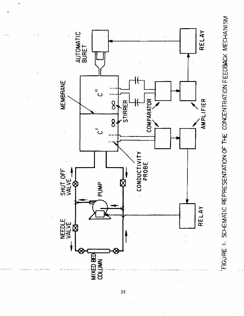
-IoQJ
QLULU
O
O
LU
Ozo
LUinLUoro_KO
UJI
LUo:ou_
24
corresponds to recent results obtained in the conductance cell described
i,n Progress Report No. 12. [The active area of the membrane (not covered2
by perforated supports) was 20.2 cm and the membrane thickness 0.017 cm].
A recent critical reexamination of the raw data from the measurements,
described in Progress Report No. 13, and observation of a progressive change
in the color of the active'areas of the membrane made it seem advisable to
remeasure the resistance. In the process of remeasurement, the procedure
was refined and additional measurements by this new procedure are in pro-
gress. (It should be noted that exact measurements of the resistance of
thin, conductive membranes are by no means a simple matter.) Results of
the newest measurements evaluated, which will hopefully be more accurate,
should be available soon.
Method for Calculation of the L-Conductance Coefficients for the M-K
Transport Equations
In the strict sense the Michaeli-Kedem ("M-K") transport equations,
(35)-(37) apply to the total system between the electrodes, i.e. the mem-
brane plus the two adjacent solutions. Since we are primarily interested
in the transport coefficients of the membrane proper, we inquire first
which of the fluxes and forces would be appreciably affected if we progressively
reduced the thickness of the solution layers in series with the membrane.
Since the solutions are well-stirred, concentration gradients in them
are negligible. Thus the generalized forces -Ays and -Auw which represent
.the chemical potential differences between the solutions near the electrodes
25
are identical with the corresponding differences across the membranes
only. As for the electrical potential difference, A<j>_, it will depend
on the magnitude of the current density, i. When the latter is zero,
A<j>_ will be independent of the position of the electrodes, and hence
the experimental A<j>_ measured at a finite distance, can be substituted
for the corresponding potential difference of electrodes in very close
vicinity of the membranes. When the current density is finite, however,
and kept constant, moving the electrodes towards the membrane will
decrease the absolute value of A<f> , since the ip drop through the solu-
tions is decreased. Therefore, if we want to calculate transport coeffi-
cients for the membrane only, without contribution of the solution layers,
we have to make allowance for this ip drop, i.e. instead of using the
measured values of A<j>_, we use the value corrected for infinitesimally
small distance from the membrane:
( across membrane = ^-'measured + P'2' + '"z"> <38>
where the p's are the specific resistances of the solutions and the z's
the distances between the membrane surfaces and the electrode surfaces
in the two solutions respectively.
This is exactly what our method of measuring the membrane conductancei*
in the cell with the movable electrodes makes possible. Moreover, when
the current is negligible (e.g. in measurements of streaming potentials
or membrane potentials),it is seen from eq. (38) that the measured potential
differences are independent of the position of the electrodes.
The celTis described "in Quarterly-Report-No. -12-
26
In a thought experiment one can reduce all the L-coefficients
to a system in which the electrodes are so close to the membrane sur-
face that the mass and ion-transfer resistances of the remaining thin
solution layers are entirely negligible. The L-coefficients calculated
for this system may be considered as the transport coefficients for the
membrane.
The methods of calculation of the conductance coefficients from
the experiments described in Table 3 are presented in this section.
The numerical calculations are in Section A. 2. of the Appendix.
When the solutions are of the same concentration and at the same
pressure, the algebraic sum of the two Ag/AgCl electrode potentials
(i.e. of the potential drops between each silver metal and the solution
in contact with it) is zero. Therefore in this case AcJ> = A<|>. Since
the conductivity of the membrane is defined as
K = H/A<j>)d (39)
if follows from eq. (37) that
1 (40)
In the determination of the membrane resistance (per unit active
area), pd, the solution resistance is eliminated by extrapolation to
zero solution thickness. Hence (Lee)A =0 1S a transP°rt characterization
The negative sign derives from the convention that for positive potentialdifference (<j>" > 4>'), the current. direction (always taken as the flowdirection of positive carriers) is negative.- _ _______
27
constant of the membrane alone. In this measurement, platinized platinum
electrodes" carrying alternating current were used, but for Ay=0 this makes
no difference, since in this case, the electric potential difference be-
tween these electrodes is the same as A<j>_.
Dividing eq. (35) by (37) for Au=0, we obtain
Lse/Lee = [Js/(1/30]Ay=0 E t+ (41)
Hence
<Lse Vo = MLee Vo <4 2>
(JSK _0 is experimentally determined in an electromigration - electro-
osmosis experiment (e.g. No. 150, Table 1). The calculation of (L e). =0
from a membrane resistance measurement has already been described [eq. (40)],
Hence L can be calculated from eq. (42).
we
Dividing eq. (36) by (37) for Ay=0, we obtain
Lwe/Lee = /^ V'O E *W C43)
Hence
(L) = tO- (44)
Thus (L ). _n can be determined from an electromigration - electroWG A|I~U
osmosis experiment, simultahedusly~with~and-simi-Tar- to the ^determi nation
of Lse.
28
LesandLew
In eq. (37) we substitute for Ay from the Gibbs-Duhem equation (9),W
and setting
= Au^ + vAp (45)
[from eq. (26), with z = 0], we obtain the following equation for theW*
electric current density
cw(46)
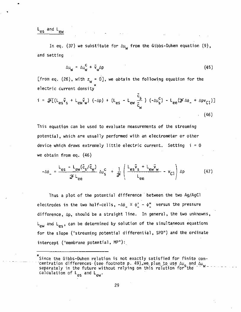
This equation can be used to evaluate measurements of the streaming
potential, which are usually performed with an electrometer or other
device which draws extremely little electric current. Setting i = 0
we obtain from eq. (46)
Ap (47)
Thus a plot of the potential difference between the two Ag/AgCl
electrodes in the two half-cells, -A<)>_ = <$>'_ - <j>" versus the pressure
difference, Ap, should be a straight line. In general, the two unknowns,
Lew and L£S, can be determined by solution of the simultaneous equations
for the slope ("streaming potential differential, SPD") and the ordinate
intercept ("membrane potential, MP"):
6S GW S W
<* ee
1 c 1-An +S ^K
L v + L ves s ew w
Lee- vci
*Since the Gibbs-Duhem relation is not exactly satisfied for finite con-centration differences (see footnote .p.. 49)_,we. plan__tp._use Ay and Ayseparately in the future without relying on this relation for thecalculation of L and L .
29
, / L v + L v~= SPD . - 1 - es s ew w .
5 MP . Les - Lew W Ayc (4g)
At the present stage of this research, we have reliable streaming
potential lines only for a system without concentration gradient (i.e.
Ay^ = 0). Such lines are shown in Figs. 2 and 3. Inasmuch as the
membrane potential is zero these data can yield only L v + L v ,es s ew wrather than L and L separately. Therefore, for the purpose of this
c o c W
interim report, we have assumed (rather than proven) that the following*
reciprocity is satisfied, as the theory demands :
Las ' Lse
Since L could be calculated from the measured transport number
of the cation [eq. (42)], L could then be calculated by rearranging
eq. (48)
*This amounts essentially to assuming that the cation transport numberdetermined by an electromigration - electroosmosis experiment agreeswith that calculated from a suitable measurement of the membrane poten-tial (17). This assumption has been made long ago for many membranes[see, for instance, (18)], although the relatively small contributionof the water transport to the membrane potential has not always beenduly taken into account.
30
UJccUJ
UJ
feQ.
LJ
0.25
< 0.20
UJo
0.15
0.10
^ 0.05
00 0.2 0.4 0.6 0.8 1.0
PRESSURE DIFFERENCE,^, aim
1.2
FIGURE 2. Streaming Potential Across C-1Q3 Membrane (Experiment 157)Solutions 0.1 M NaCl. Short vertical and slanted lines connectingpoints referring to same pressure setting indicate hysteresis effectafter removal and re-application of pressure. All points correctedfor small asymetry potentials between Ag/AgCl electrodes separatedby the membrane, observed at the time of pressure release.
31
LulOzUJct:LJ
LJ
CL
UJ
0.20
0.15
Ox
0.10
E 0.05I-oLU
00 0.2 0.4 0.6 0.8 1.0
PRESSURE DIFFERENCE, Ap,otm
FIGURE 3. Streaming Potential Across C-103 Membrane (Experiment 162)Solutions 0.1 M NaCl. Pressure was increased in steps without inter-mediate pressure release after each step. Line is corrected for smallinitial asymetry potential between Ag/AgCl electrodes separated by themembrane.
32
) - Lse5s] (52)
In this manner we tested the reciprocity relation
and found it to hold within six percent over the limited pressure
range investigated (up to Ap = -1 atm). The numerical calculations
are presented in Appendix 2.
In the future we plan to measure streaming potential curves (in-
cluding measurements at Ap=0, i.e. membrane potential measurements) for sys-
tems with a concentration gradient. The assumption L = L can theno C Co
be tested experimentally.
Lss' Lww' Lsw and Lws
These remaining four coefficients can in principle be calculated from
the following four ratios of flux to driving force:
)._ n A n Osmotic water flux (osmosis -*-»• dialysis experiment)W 51 *™U jtip"~U
(J /Avr). 0 A 0 Dialytic salt flux (osmosis -*-»• dialysis experiment)
(J /Ap)^_n Water flux (hyperfiltration experiment)W I "~U
(J /Ap)-_Q Salt flux (hyperfiltration experiment)
The first three of these measurements can be performed in the present
"concentration-clamp" apparatus, but the accurate determination of the
salt flux due to a pressure difference is not possible in this apparatus
33
which for a number of good reasons was built from a translucent poly-
carbonate plastic. The latter is not mechanically stable at pressures
high enough to measure the salt-filtering effect in hyperfiltration
("reverse osmosis") with a reasonable degree of accuracy . Therefore
we assume, rather than prove, that L = L ; as a result we have only5W W5
three unknowns to be determined from the first three measurements.
The relevant equations are derived in the following.
For i=0, we rearrange eq. (37) as follows:
-(#Ac}>_ - vclAp) = j-Si Ays + £§* Ayw (54)ee ee
Applying this equation to the calculation of the salt flux in a
dialysis «-»• osmosis experiment (where i=0) from eq. (35) in which we
substitute -(v.Ap + Ay?) = -Ay. for the first two driving forces,
Since the dialysis •«-*• osmosis experiment is performed at uniform
pressure, this reduces to
/ Js
K_ i' Lss
1=0Ap=0
L Lse es +
Lee
L L. es ewsw .
ee
(56)
The principal investigator has at his disposal a complete tubular hyper-filtration apparatus in.which this, salt rejection effect is being measuredsimultaneous with the hyperfiltration rate ancl withf streaming potentials-across modified cellulose acetate membranes at pressures up to 100 atm (19).This apparatus is in use for another project, however, and would have to bemodified to provide the data necessary here, and this could not be done in the past.
34
The determination of L and L has already been described--- - _ CC CW
see eqs. (40) and (52) respectively. Lgs could not be determined by
experiments, but has been assumed equal to L [eq. (42)] in view ofSc
the reciprocity relation (50). The salt flux, (J c )^_n A__ n wasS 1 U j AP"~U
determined in the dialysis experiment. Hence the only two unknowns
in eq. (56) are l_ss and l_sw.
In the same manner we obtain from eq. (36) for the water flux:
C57)
Since the pressure is uniform, this reduces to
/ oww
we ew ,
Leews
we es
Lee ;
(58)
The unknowns in this equation are L and LW$ .
To evaluate the hyperfiltration experiment, we divide eq. (57) by -Ap:
-L v +wsss -- + L v + es "es s ew
Ap Ap+ L v )ew w'
(59)
The water flux, J , is measured as a function of the pressure difference,w-Ap. The unknowns in this equation are L and L .
WS WW
Thus it is possible to determine the three unknowns , LWS= LSW and
L$s by solution of the three equations (56), (58) and (59), provided all
*Note that the method of calculation for L has already been 'described [eq-. (44)-].We
35
experiments were performed under the same concentration gradient.
Our hyperfiltration experiments were performed at conditions of
uniform concentration (i.e. y£ = 0 = y^; no osmosis) by "clamping"
the concentrations of the two solutions adjacent to the membrane at
equal concentrations of about 0.1 M KC1. For this case eq. (59)
reduces to the simple form
0 = ("-wsVo *s + (LwwVo *w ' (Lwe/LeeVoAp=0
(60)
In principle it is not permissible to solve the triplet of
equations (56), (57) and (60) for L, L = LC1(, and Lcc, because theww ws sw ss
first two equations refer to a dialysis experiment which, by definition
requires a concentration gradient, while the last equation refers to
an experiment at uniform concentration. In the future,we plan to main-
tain the finite concentration difference in all experiments (as we have
indeed occasionally done in the past), but for the purpose of this report
we shall utilize the results of the latest measurements, as presented in
Table I, in which the water flux under pressure was measured under con-
ditions of Ay=0. Since L is similar to a d'Arcy permeability constant,WW
and since it is known that these "constants" vary but little with concen-
tration (provided the concentration is below about 1 M), we do not think
that the value of L^ would have been appreciably different if the concen-
trations of the solutions in the hyperfiltration experiment had been identi*
cal with those in the dialysis «-»• osmosis experiment . In fact it
The water flux, as opposed to the coefficient L^ would change very appre-ciably, however, .since, in addition to the pressure force, the osmoticforce would drive the water through the membrane.
36
is usually tacitly assumed that the conductance coefficient L is
independent of the concentrations of the solutions bracketing the
membrane (1). As for the coefficient L = L , some dependence onws sw
the solution concentrations is expected (20), but this dependence is
neglected in this report. Consequently, the three coefficients L ,Li,c = Lcl. and L are determined by solution of the simultaneousWo SW So
equations (56), (58) and (60). The calculations are presented in
part A. 2. of the Appendix. The results of the calculations of all
conductance coefficients in the M-K matrix are presented in Table 4.
Conclusions
While it is not easy to draw immediate conclusions on the transport*
mechanism from the phenomenological conductance coefficients, L , several
important points emerge from consideration of the L-values in Table 4 and
the methods used to calculate these values:
First, the coefficients related to a larger extent to the solvent
than to the salt are larger Uew » Lgs; L^ » LW$; L$w » LSS). This
is probably due to the much higher concentration of water than of salt
in the ion-exchange membrane, for the coefficients L. . increase in general' J
with increasing c. [while the flux equations in ref. (8) are not identicalJ
with equations (35)-(37) used here, some insight into the physical meaning
of the L-coefficients, and in particular the above conclusion about their
*On the other hand, friction coefficients, which can be calculated from thecomplete group of L-coefficients are useful for this purpose (8-10). Weplan to perform such calculations in the future. We expect that it will
- be~useful to invert-the flux-force equations-first, -i.e. -present- the .forcesas sums of terms linear with respect to the fluxes, and calculate the frictioncoefficients from the resulting resistance coefficients, R —
1 ' J
37
TABLE 4
Phenomenological Coefficients for System 0.05 N NaCl lc-103 I 0.1 N NaCl
These conductivity coefficients, L, refer to the flux equations (35)-
(37). All coefficients have the units joule" mole cm sec1 Jd"
"ee
'se
"we
"ew
ws
"ss
ww
1.89 x 10_1]***
1.64 x 10⁻¹¹***
1.88 x 10_10***
1.77X10"10*
1.73 x 10"10
**
1.42 x 10"
1.31 x 10⁻⁸
L assumed equal to Les se
reciprocal pair
L assumed equal to Lws
Cation-exchange membrane made by American Machine and Foundry Company,Stamford, Connecticut.
** 31 joule = 1 wattsec = 1 dekabar cm .
***Determined from measurements on system without concentration gradient,0.1 N NaCl | C-103 | 0.1 N NaCl.
38
variation with c. (borne out by the results) may be obtained from thatJ
reference; see eqs. (17) or (32) of reference (8)]. This property of
the set of L-coefficients thus probably reflects the exclusion of salt
from the ion-exchange membrane ("Donnan effect").
Second, one of the three reciprocity relations was tested by the
results of our experiments, and was confirmed within about six percent
for the conditions used in these measurements.
Third, the numerical calculations in section A. 2. of the Appendix
show the large dependence of all L-coefficients on the membrane conductance
(Figure 4). In fact, membrane conductance emerges as the most decisive
transport characteristic, thus justifying a posteriori the time-honored
decision of battery technologists to use conductance measurements as pri-
mary screening tests for separator materials. The implication of this
conclusion for future experiments is the emphasis on refinements of the
technique of membrane conductance measurements. A more elaborate and more
accurate technique than the one used in the past is being developed. It
uses the existing apparatus described in Progress Report No. 12. Apparatus
and procedure were modified to yield much more accurate measurements of
the distances of the electrodes from the membrane. In case future measure-
ments yield a somewhat different conductance value, all L-coefficients in
Table 4 will be different, but their ratios will not change much.
Fourth, consideration of the numerical values of all terms in the
calculation of the conductance parameter, LSS, which relates the rate of
electrolyte diffusion through the membrane to the "electrolyte diffusion
force."., _-Ay _, „(determined by .the^concentration gradient of the electrolyte)
39
Without Membrane
DISTANCE, cm
FIGURE "4. C-103~Membrane7 "Evaluation" of Resistance (25°C). "Solution 0.1 N NaCl. Active area = 20.25 cm . Abscissa repre-sents distance from point of closest approach of electrodes tomembrane' (upper line) or electrode distance (lower line). Re-sistance of membrane is determined from ordinate distance ofthe two parallel lines. For lower line ordinate intercept rep-resents circuit impedance. ,
40
leads one to the conclusion that osmosis +->• dialysis with shorted electrodes
(rather than with unconnected electrodes) should be tried, in an attempt
to improve the accuracy of this determination. Also it would be worth-
while to investigate under what conditions, if any, the planned, simul-
taneous application of several independent forces improves the accuracy
of the determination of the conductance coefficients, L.
Finally, the methods developed here for calculating a set
of L-coefficients from specified transport measurements lead to the unequi-
vocal characterization of any system of the type: solution membrane | solution,
provided only that these specified measurements can be performed with suf-
ficient accuracy. The "concentration-clamp" apparatus developed in this
project represents a large step towards the attainment of this experimental
aim; the following next steps are desirable: (a) further refinements of
the apparatus and procedure in order to obtain this desired accuracy in a
few types of transport measurements in which we still need these improve-
ments, and (b) the systematic collection of transport data.
Acknowledgement
The Principal Investigator and his collaborators thank Mrs. J. Worthington
for her valuable editorial help.
41
APPENDIX
A. 1. Relation of electrical potential difference, A<j>, across the membrane^to potential difference, Aft., between two Ag/AgCl electrodes.
Consider the isothermal system
Ag/AgCl Nad solution, c', p1 Membrane Nad solution, c", p' Ag/AgCl
The condition for equilibrium between each solution and the Ag/AgCl*
electrode in contact with it is that the sum of the total potentials
of the reactants equals that of the products. The electrochemical electrode
equilibrium is
Ag + Cl~^ AgCl + e" (Al-4)
where e" stands for one mole of electrons in the silver metal. Thus the
equilibrium conditions for the two electrodes respectively are
The total potential of component i, y^ is the sum of the contributions ofthe pressure-dependent, concentration-dependent, and electric field-dependentparts of the (chemical) potential (12, p. 94, 469, 480)
vlj = y + (P - 0.1013) v1 + RTlnai + z^. (Al-1)
Mp^fwhere ft. is the standard potential, z- the valency of the particle (+1 for+ -Ag , -1 for Cl , zero for species carrying no appreciable net charge, e.g.
Ag and AgCl ) and <j> the electrical potential (volt) at the locations considered:
= yAgCl
and similarly for silver:
Note that the pressure is measured in dekabar (0.1013 dekabar = 1 atm)
42
ii" + fi"yAg yCl= ii
- uiAgCl
n (Al-5)
(Al-6)
Subtract (Al-6) from (Al-5)
AV (Al-7)
Because of the small volume of the (non-hydrated) electrons,the .
effect of pressure on the total potential of the electrons is assumed to
be negligible. Also, since the electron concentration in the wire,and
hence yj .are nearly uniform, it follows from (Al-1) that
Ay (= Ay - 3 Acj> ) - - Atf) (Al-8)6 c ~ ™
where A<J> is the electrical potential difference between the electrodes.
Substitute for Aye_ in eq, (Al-8) from (Al-7)
Aye- = - = Aycl_ - - Ay.J (Al-9)
According to "Poynting's equation" (12, p. 304), the variation with
pressure of the free energy of one mole, G^/h^ of a pure component i,
is related to the total volume, V.., of n.. mole of this component by:
9p • Vni (Al-10)
Applying (Al-10) to pure AgCl and Ag respectively, we obtain:
/"AgClIT- =_ AyAgCl_ (Al-11)
43
Here we have used the fact that, by definition of the partial molar
quantities, the molar free energies, G./n- and the molar volumes V./n^
of pure substances are identical with the partial molar free energies,
y., (chemical potentials) and partial molar volumes, v^, respectively.
Substituting AyA c, ar]d AyA ^rom (A!-11) and (Al-12) respec-
tively in (Al-9), we obtain
AV = -3^_ = Aycr - Ap(vAgC1 - VAg) (A
Therefore the potential difference, A<j>_, between the two Ag/AgCl
electrodes is
A* = -(l/^)[Ay f l- - Ap(vA n - V. )] = -u i *»y^' i »»y — •
where the symbol vcl replaces (VA pi ~ VA ) and symbol y_ replaces
Ur-i-» for the sake of brevity.
Comparison of this result with equation (12-6) p. 150 of ref. (2) shows
that in the latter, the term AP(VA C1 - VA ) has been neglected.
Let us examine to which extent this term affects the evaluation of
the results of our experiments. To do so, we calculate first the numeri-
cal magnitude of the expression Ap(vA -.-j - VA ):
From ref. (13), p. 648, the specific gravity and molecular weight3
of silver are 10.5 g cm and 107.88 respectively. Hence
- ^-107.88. g,mole"1 = 10 28 ° "A9 " 10.5 gem'3
44
143 34 3 -1and, from the same source v. r, = = 25.8 cm moleAgu 5.56
Hence -j>Ap(vAgC]
J r (25.8 - 10.28) cm3 mole"1 Ap
0.965 x 10 amp sec eq s ^ '-15.5
For Ap = -0.2 dekabar (about 2 atm) this yields
(*Aori - VA>P - 1 - 6 1 x ""O" x °-2 = 3.22 x lO'5 volt& 9 9 amp sec
i.e. -0.032 millivolt for 2 dekabar.
The streaming potential for the C-103 membrane considered in this
report was more than one order of magnitude higher. We conclude that as
a very first approximation, eq. (12-6) of ref. (2) may be used, but that
the correction term Ap(vA cl - v. ) is not entirely negligible.
Returning to eq. (Al-14), we substitute for Ay^- in terms of
the definition of the total potential [eq. (Al-1)]:
Ap(vAgC1 - vAg)]
vAg
45
Now, if the volume change in the electrochemical reactions at the
electrodes [eq. (Al-4)] is negligible, then the last term of equation
(Al-15) is negligible (15b).*
Therefore :
14 _ * -(Ay./^) + A* (
One can calculate the potential drop across the membrane, A<f>,
which represents the difference in electrical potential between the
two solutions in the immediate vicinity of the membrane surfaces. by
simply adding a "concentration correction", (Ay£,_/£0 = (RT/ OlnUp..-
to the potential difference, A<J>_, measured between the Ag/AgCl electrodes
£4 - A<f>_ + (Ayr./3f) (AT -17).
A(j> appears as a component of the general driving force of the Onsager
set of flux equations (3)-(5). Note that eq. (Al-17) was presented (without
proof) in the 1968 Annual Progress Report.
Note that this term is likely to be much smaller than the term Ap(v^ cl - v. )discussed in connection with eq. (Al-14). 9 9
46
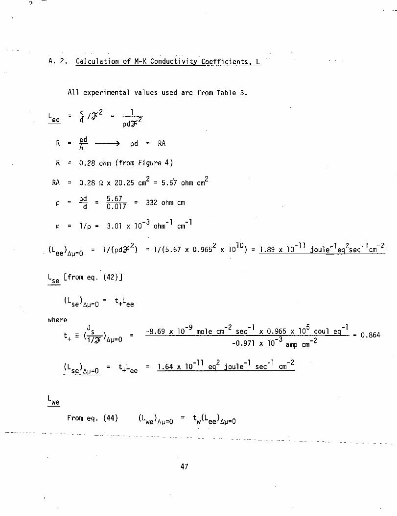
A. 2. Calculation of M-K Conductivity Coefficients. L
All experimental values used are from Table 3.
= jp pd = RA
R =
RA =
p =
< =
0.28 ohm (from Figure 4)
o o
0.28 n x 20.25 cm = 5. 67 ohm cm
OT7 = 332 ohm cm
1/p = 3.01 x 10"3 ohm"1 cm"1
(Lee)A]J=0 = l/(5.67 x 0.9652 x 1010) = 1.89 x 10"11
L [from eq.(42)]se
where-8.69 x 10"9 mole cm"2 sec"1 x 0.965 x 10 coul eg
(Lse)Ay=0 t+Lee
_
-0.971 x 10 amp cm
= 1.64 x IP"11 eg2 joule"1 sec"1 cm"2
O"2
we
From eq. (44) 'Ay=0 " VLee'Ay=0
47
where
t , = I J,,/ ( i ar ; j AW W 'JAy=t E [J /(iSK)] = "99-79 x 10"9 mo1e cm"2 sec"1 x 0.965 x 105 coul eg"1 _ g g2
0.971 x 10 amo cm"
(Lwe)Ay=Q = twLee = 9.92 x 1.89 x 10"11 = 1.88 x IP"10 joule"1 eg2 sec"1 cm"2
ew
From eq. (52) :
<LewVo ' rW
From streaming-potential line.SPD = 0.176 x 10"3 f- x 9.87
SPD = 1.737 x 10"3 volt dekabar"1
(Lew )Ay=0 = TO?1"0168 Cm" °'965 X 10' COUl mole" 1.898 x l(f3
/ 3 - 1 * *i ? 1 9 1 15.5 c m mole
~ ' r.^^-<-r./-~ I m~^- ix 1.89 x 10 " joule 'eq'sec 'cm fc. '1.737 x 10 J volt dekabar ' + Q>965 x 1Q5coul
- 1.64 x 10"11 eq^oule^sec'^m"2 x 17.2 cm3 mole"1***!
(Lew)Ay=Q = ^i^ [348 x 10"11 - 28.2 x 10"11] = 1.77 x IP"10 Jou1e"1mo1e2cm"2sec"1
* 1 dekabar = 10 bar = 9.8 atm. This unit was introduced (8-) because iteliminates conversion factors when all electrical and osmotic measurementsare expressed in units containing the practical wattsec = joule (1).
**From appendix A.I.
Ref. 21, p. 250, eq. (8-5-4). Parameters for equation from p. 253, Table 8-5-1
48
Lww» Lws' = Lswand Lss
To calculate these coefficients (all at Ay ^ 0), we first calculate
Aus and Ay^.
c£ = l.OOlg x 10"4 mole cm"3 (= O.lOOlgN)
c' = 0.495. x 10"4 mole cm"3 (= 0.0495,N)
The mean activity coefficients, y+» of Na (or Cl~) are obtained by
interpolation from ref.(22, Appendix 8.9, p. 466 ). Since the solutions are
rather dilute, ratios of molar concentrations are sometimes substituted for
ratios of molality throughout the following calculations:
c1 = 0.0495 x 10"3 mole cm"3(m' = 0.0497 mole NaCl/1000 g H2Q, Jm = 0.223); y± = 0-821
c" = 0.1001 x 10"3 mole cm"3(m" = 0.1005 mole NaCl/1000 g HgO.'yfiT* 0.317); y+ = 0.780
[a!/aj= C'Y;/(C"Y") = (0.0497 x 0.821)7(0.1006 x 0.780) = 0.52i s S/.J. - -
y^ = RTln(a^/a;)2 = 2 x 8.13 joule mole"1(°K)"1 x 298(°K)[-ln(0.52)] = 3169 joule mole"1
0.65393
The water activities are found by linear interpolation of published data
(ref. 22, Appendix 8.3).
Comparison with other references" showed-that--the-term, "activity coefficient ofelectrolyte" used in the heading of this table stands for the mean'activity -coefficient, y±> of the Na+ ions (equal to the mean activity coefficient of theCl- ions). The activity coefficient of the salt, YNaC1» equals Y± (14, Table 1)
49
m = 0.0497 mole NaCl/1000 g hLO: a1 = 0.998332
m = 0.1006 mole NaCl/1000 g H20: a" = 0.996626
~1 "1= -8.13 joule mo1e~{deg K)" x 298 K x (0.001706/0.997)
c -1*Ay = -4.15 joule mole
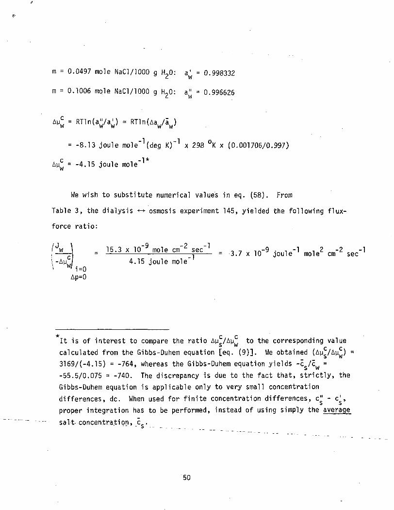
We wish to substitute numerical values in eq. [58). From
Table 3, the dialysis •*-> osmosis experiment 145, yielded the following flux-
force ratio:
/Jw
1
i=0!\p=0
_ 15.3 x 10"9 mole cm"2 sec"1
4.15 joule mole"1Q-9 JQule-l cm-2 sec-l
* c cIt is of interest to compare the ratio Au /Au^ to the corresponding valuecalculated from the Gibbs-Duhem equation [eq. (9)]. We obtained (Ay^/Ay^) =3169/(-4.15) = -764, whereas the Gibbs-Duhem equation yields -c/c1( =5 W
-55.5/0.075 = -740. The discrepancy is due to the fact that, strictly, theGibbs-Duhem equation is applicable only to very small concentrationdifferences, dc. When used for finite concentration differences, c^ - c^,proper integration has to be performed, instead of using simply the averagesalt concentration, cg.
50
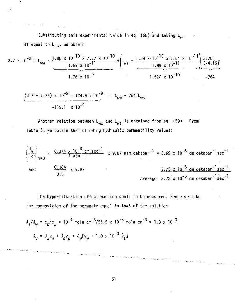
Substituting this experimental value in eq. (58) and taking L
as equal to L , we obtain
3 7 x 10"9 = L x 1' X lt88 x 1.64 x
1.89 x 10-11 WS 1.89
1.76 x 10"9
1.627 x 10"10
3170
-764
(.3.7 + 1.76) x 10~9 - 124.6 x 10"9 = L, - 764 Lj W W W o
---- — -------- ,- " " • •
-119.1 x 10~9
Another relation between L and L is obtained from eq. (59). From
Table 3, we obtain the following hydraulic permeability values:
-APM=O= 0-374 x 10" cm sec~ I
and0.8
1 atm
x 9.87
atm dekabar-l = 3>69 x 1Q-6 cm
3.75 x IP"6 cm dekabar'^ec"1
6 V IAverage 3.72 x 10 cm dekabar sec
The hyperfiltration effect was too small to be measured. Hence we take
the composition of the permeate equal to that of the solution
Jc/J,, = cc/c,, = 10~4 mole cm"3/55.5 x 10"3 mole cm"3 = 1.8 x 10"35 W S W
Jv =
51
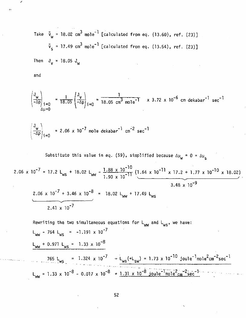
Take v = 18.02 cm3 mole"1 [calculated from eq. (13.60), ref. (23)]
v = 17.49 cm3 mole"1 [calculated from eq. (13.54), ref. (23)]
Then J = 18.05
and
w-Ap i=Q 18.05 [ -Ap
Ay=0
1
i=0 18.05 cm mole" x 3.72 x 10"6 cm dekabar"1 sec"1
w : = 2.06 x 10"7 mole dekabar"1 cm"2 sec"1
i=0
Substitute this value in eq. (59), simplified because Ay = 0 = Ay
2.06 x 10"7 = 17.2 Lws + 18.02 1t88 X 10 11 (1.64 x 10"11 x 17.2 + 1.77 x 10"10 x 18.02)1.90x10"" N /
3.48 x 10⁻⁹
2.06 x 10"7 + 3.46 x 10"8 = 18.02 l_ww + 17.49 LWS
2.41 x 10⁻⁷
Rewriting the two simultaneous equations for L and L , we have:WW WS
-7L - 764 L = -1.191 x 10WW WS
L in i + 0.971 L = 1.33 x 10"8
WW WS
765 I = 1.324 x 10"7 ->• L.C(=LCJ = 1.73 x 10"10 joule"1mole2cm"2sec"1
— — - Wd Wi> o W
L = 1.33 x 10"8 - 0.017 x 10"8 = 1.31 x IP"8 Jou1e"1mo1e2cm'''2se'c"1""' "ww '
52
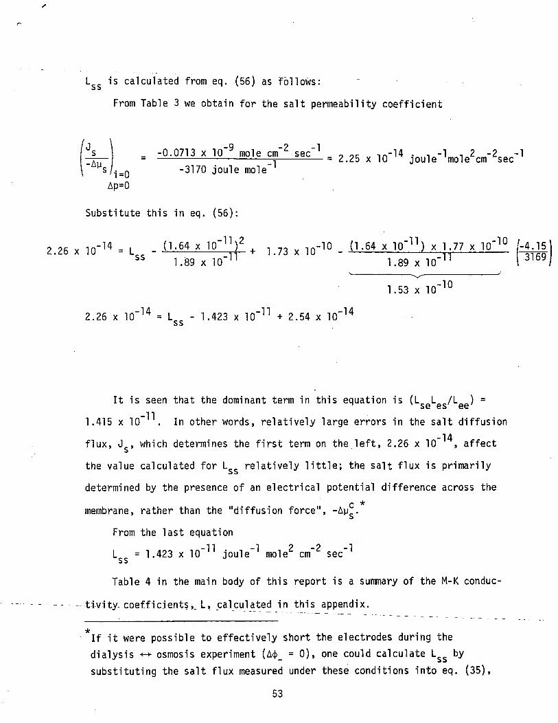
L is calculated from eq. (56) as follows:
From Table 3 we obtain for the salt permeability coefficient
-0.0713 x 10"9 mole cm"2 sec"1 0 oc ,rt-14 . , - 1 , 2 - 2 -1= 2.25 x 10 joule mole cm sec-Ay -3170 joule mole"Ap=0
Substitute this in eq. (56):
2 26 x 10"14 = L - d-64 x IP"11)2 . ,--10 _ (1.64 x IP"11) x 1 77 x IP"10C.tU A IU L J r t T I./O X IU JT-* -
SS 1.89 x 10 M 1.89 X 10 " 1
1.53 x 10"10
2.26 x 10"14 = Lss - 1.423 x 10"11 + 2.54 x 10"14
It is seen that the dominant term in this equation is (L L /L ) =OC CO CC
1.415 x 10" . In other words, relatively large errors in the salt diffusion
flux, J , which determines the first term on the left, 2.26 x 10" , affect
the value calculated for L relatively little; the salt flux is primarilyj o
determined by the presence of an electrical potential difference across thec *membrane, rather than the "diffusion force", -Ays-
From the last equation
LSS = 1.423 x 10"11 joule"1 mole2 cm"2 sec"1
Table 4 in the main body of this report is a summary of the M-K conduc-
tivity-coefficients,. L, calculated in this appendix.
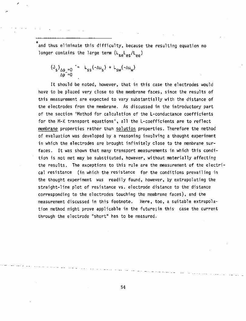
If it were possible to effectively short the electrodes during thedialysis •*-»• osmosis experiment (A<j>_ = 0), one could calculate Lgs bysubstituting the salt flux measured under these conditions into eq. (35),
53
*arid thus eliminate this difficulty, because the resulting equation nolonger contains the large term (L L /L )
oG C d v*v*
Ap"=0
It should be noted, however, that in this case the electrodes wouldhave to be placed very close to the membrane faces, since the results of
this measurement are expected to vary substantially with the distance ofthe electrodes from the membrane. As discussed in the introductory partof the section "Method for calculation of the L-conductance coefficientsfor the M-K transport equations", all the L-coefficients are to reflectmembrane properties rather than solution properties. Therefore the methodof evaluation was developed by a reasoning involving a thought experimentin which the electrodes are brought infinitely close to the membrane sur-faces. It was shown that many transport measurements in which this condi-tion is not met may be substituted, however, without materially affectingthe results. The exceptions to this rule are the measurement of the electri-cal resistance (in which the resistance for the conditions prevailing inthe thought experiment was readily found, however, by extrapolating thestraight-line plot of resistance vs. electrode distance to the distancecorresponding to the electrodes touching the membrane faces), and themeasurement discussed in this footnote. Here, too, a suitable extrapola-tion method might prove applicable in the futurejin this case the current
through the electrode "short" has to be measured.
54
REFERENCES
(1) J. G. McKelvey, Jr., K. S. Spiegler and M. R. J. Wyllie, Chem. Eng.Progr. Rep. Symposia Series 55_ (No. 24), 199 (1959).
(2) A. Katchalsky and P. Curran, "Non-Equilibrium Thermodynamics forBiophysicists", Harvard University Press, Boston, Mass., 1966.
(4) L. Onsager, Annals New York Acad. Sci. 46_, 24 (1945).
(5) R. M. Barrer in "Membrane Phenomena", Disc. Faraday Soc. 21, 138-9(1956). ~~
(6) K. S. Spiegler, Ind. Eng. Chem. (Fundamentals) 5_, 529 (1966).
(7) F. Helfferich, "ion Exchange", McGraw Hill, New York (1962).
(8) K. S. Spiegler, Trans. Faraday Soc. 54_, 1408 (1958).
(9) I. W. Richardson, Bull. Math. Biophys. 3£, 237 (1970); J. MembraneBiol. 4_, 3 (1971).
(10) P. Meares, J. F. Thain and D. G. Dawson, "Transport Across Ion-ExchangeMembranes; The Frictional Model of Transport", Ch. 2 in "Membranes",G. Eisenman, ed., Marcel Dekker, Inc., New York, 1972.
(11) B. C. Duncan, (a) J. Res. National Bureau Standards, 66A, 83 (1962);(b) "Progress Report for Membrane Characterization Work", December31, 1965.
(12) G. N. Hatsopoulos and J. H. Keenan, "Principles of General Thermo-dynamics", J. Wiley and Sons, New York, 1965.
(13) C. D. Hodgman, ed., "Handbook of Chemistry and Physics", 43rd ed.,Chemical Rubber Publishing Co., Cleveland, Ohio, 1961.
(14) K. S. Spiegler and M. R. J. Wyllie, "Electrical Potential Differences",Ch. 7 in "Physical Techniques in Biology", 2nd ed., Vol. II, D. H. Moore,ed., Academic Press, New York, 1968.
(15) (a) I. Michaeli and 0. Kedem, Trans. Farad. Soc. 5J7_, 1185 (1961);(b) 0. Kedem and A. Katchalsky, ibid. 59_, 1918 (1963).
(16) A. Zelman, J. C. T. Kwak, J. Leibovitz and K. S. Spiegler, "The Concentration-_ . j;iamp Method for Transport Measurements in Membranes", in "Biological Aspects
(17) G. Scatchard, J. Amer. Chem. Soc. 75_, 2883 (1953).
(18) K. Sollner, J. Electrochem. Soc. 9_7, 139C (1950).
(19) Saline Water Conversion Report 1970-71, Office of Saline Water,U. S. Department of the Interior, p. 335; obtainable fromSuperintendent of Documents, Washington, D.C. 20402.
(20) K. S. Spie.gler and 0. Kedem, Desalination ]_, 311 (1966).
(21) H. S. Harned and B. B. Owen, "The Physical Chemistry of Electro-lytic Solutions", 2nd ed., Reinhold, New York (1952).
(22) R. A. Robinson and R. H. Stokes, "Electrolyte Solutions", Butterworths,London, 1955.
(23) I. M. Klotz, "Chemical Thermodynamics", Revised edition, W. A.Benjamin Co., San Francisco (1964).