Abstract This paper develops a new pair trading method to detect inefficiencies inexchange ratesmovements and arbitrage opportunities using a convergence/divergenceindicator (CDI) belonging to the oscillatory class. The proposed technique is applied to11 exchange rates over the period 2010–2015, and trading rules based on CDI signalsare obtained. The CDI indicator is shown to outperform others of the oscillatory classand in some cases (for EURAUD and AUDJPY) to generate profits. The suggestedapproach is of general interest and can be applied to different financial markets andassets.
Pair trading is a technique often used by practitioners to predict short-term pricemovements and detect arbitrage opportunities. It searches for statistically linked assetpairs and any mis-pricings that can be exploited through arbitrage trading until thedivergence in prices disappears.
This paper develops a new pair trading method to detect inefficiencies in exchangerate dynamics and arbitrage opportunities that is based on a convergence/divergenceindicator (CDI) belonging to the oscillatory class. The proposed technique is appliedto 11 exchange rates over the period 2010–2015, and trading rules based on CDIsignals are obtained. The suggested approach is of general interest and can be appliedto different financial markets and assets.
The basic idea is as follows: the degree of correlation between financial assetsvaries over time, and can be very high in certain periods. For example, the averagecorrelation between EURUSD and AUDUSD in 2015 has been higher than 0.9 atthe daily frequency, and in the range [0.8–0.9] if considering hourly intraday data,but at times the hourly correlation has dropped below 0 and even below −0.5 beforereverting to “normal” values. We investigate the reasons for such abnormal situationsin the case of the FOREXmarket using a convergence/divergence indicator (CDI) andshow its efficiency in comparison to other popular methods.
The layout of the paper is as follows. Section 2 briefly reviews the literature ontechnical analysis. Section 3 describes the data and outlines themethodology. Section 4presents the empirical results, while Sect. 5 offers some concluding remarks.
2 Literature Review
Forecasting asset price movements is a challenging task. According to the EfficientMarket Hypothesis (EMH—see Fama 1970), prices should follow a random walk.However, several studies have tried to detect exploitable profit opportunities whichwould constitute evidence of market inefficiencies. Statistical arbitrage is a very pop-ular trading strategy that was first used by Morgan Stanley in the 1980s (see Gatevet al. 2006 for details). It can be described as follows: the investor selects a pair ofassets for which the mean spread between prices is relatively constant, and in caseof deviations from this value he keeps selling one asset and buying the other till thespread reverts to its equilibrium level; then opened positions are closed.
This method was subsequently analysed in academic studies (Burgess 1999; Bon-darenko 2003; Hogan et al. 2004, etc.), mainly for stock markets (Hong and Susmel2003; Nath 2003; Gatev et al. 2006; Perlin 2009; Do and Faff 2010; Avellaneda andLee 2010; Broussard and Vaihekoski 2012 and others). There is plenty of evidencethat pair trading allows to generate abnormal profits in various financial markets, forinstance in the US (Gatev et al. 2006) and Finnish (Broussard and Vaihekoski 2012)stock markets. This approach was further investigated by Enders and Granger (1998),Vidyamurthy (2004), Dunis and Ho (2005), Lin et al. 2006 and Khandani and Lo(2011) among others. A variety of methods have been used for statistical arbitrage,including: cointegration analysis; correlation analysis; regression analysis; neural net-works; pattern recognition methods; factor models; subjective approaches (when thetrader/investor selects pairs based on their fundamentals or other characteristics whichmake them “similar”—see Vidyamurthy 2004 for details).
Standard cointegration tests (see Engle and Granger 1987; Johansen 1988) are fre-quently carried out to devise trading strategies based on long-run linkages betweenasset prices. However, these might not be particularly useful in the presence of struc-
123
Searching for Inefficiencies in Exchange Rate Dynamics 407
Fig. 1 Daily data, EURUSD, 2014
tural change. For instance, the correlation between oil andEURUSDwas−0.7 in 2005,but 0.9 in 2007–2008, the average for the period 2005–2008 being in the 0.7–0.8 range.Clearly, statistical arbitrage based on cointegration analysis will not work in such acase. In fact Capocci (2005) found that during the financial crisis of 2007–2009 fundsemploying a pair trading strategy did not perform well. One possibility is to use inperiods of instability the Kalman filter (see Dunis and Shannon 2005). The alternativeis correlation analysis focusing on the short-run statistical properties of asset prices(see Alexander and Dimitriu 2002).
Once profitable trading strategies become well-known to the financial community,they cease to generate profits (see Chan 2009). Indeed Gatev et al. (2006) have shownthat returns from pair trading strategies have been declining over time. Thus, it isimportant to develop new techniques, which is the aim of this paper.
3 Data and Methodology
Correlation analysis is a very popular method in financial markets, especially in stockmarkets (the degree of correlation between the S&P 500 and Dow Jones indices ishigher than 0.9), less so in the FOREX market because linkages between currencypairs are much more volatile, as can be seen in Figs. 1 and 2 in the case of EURUSDand AUDUSD in 2014.
However, this was not the case in 2013 (see Figs. 3, 4).Annual correlations are reported in Table 1.As can be seen, the two series are generally positively and strongly correlated, but
their correlation can suddenly become negative as it did in 2013, when it dropped to−0.41. Correlations for other financial assets are reported in Table 2, which confirmsthat from time to time divergence can occur [more information about correlationsbetween financial assets can be found in Plastun and Kozmenko (2011)]. The questionarises whether this type of information can be used to predict future price movements.
123
408 G. M. Caporale et al.
Fig. 2 Daily data, AUDUSD, 2014
Fig. 3 Daily data, EURUSD, 2013
In this paper we focus on exchange rate dynamics. Having discussed the cases ofthe EURAUD and AUDUSD rate as an example, we then move on to the remainingrates.
Let us consider first the dynamics of EURUSDandAUDUSDover the period 20–23February 2015 (see Fig. 5). The daily correlation between the two series wasmore than0.9 (see Fig. 6) and positive, but on 20 February, at 8pm prices started to move in theopposite directions, before converging again on 23 February at 3am. Specifically, thehourly correlation dropped to −0.8 before reverting a few hours later to its “typical”range 0.8–0.9 (see Fig. 7).
The biggest negative hourly correlation (−0.96) occurred at 2pmon20February, thedaily correlation being instead strongly positive (0.9—see Table 3 for details). Duringthis period EURUSD fell and AUDUSD rose. This would suggest that a trader should
123
Searching for Inefficiencies in Exchange Rate Dynamics 409
Fig. 4 Daily data, AUDUSD, 2013
Table 1 Correlations betweenEURUSD and AUDUSD in2004–2014
Year Correlation
2004 0.71
2005 0.81
2006 0.78
2007 0.88
2008 0.96
2009 0.98
2010 0.58
2011 0.81
2012 0.47
2013 −0.41
2014 0.76
Table 2 Correlation analysis for different financial assets in 2005 and 2008
Financial assets EURUSD USDJPY AUDUSD
2005 2008 2005 2008 2005 2008
Oil futures −0.66 0.82 0.62 −0.55 −0.37 0.84
Gold spot −0.63 0.27 0.83 −0.49 −0.56 0.39
US Stock market (Dow Jones Index) −0.13 0.11 0.26 0.32 −0.11 0.15
buy EURUSD at 1.1313 and sell AUDUSD at 0.7841 till the anomaly disappears(at 3am on 23 February), and then any open positions should be closed by closingEURUSD at 1.1386 and AUDUSD at 0.7834. This generates a profit of +0.65 % forEURUSD and +0.09 % for AUDUSD, and therefore an aggregate profit of +0.73 %.
123
410 G. M. Caporale et al.
Fig. 5 Hourly price dynamics of EURUSD and AUDUSD on 20–23 February 2015
0.860.865
0.870.875
0.880.885
0.890.895
0.90.905
0.91
02-0
2-20
15
04-0
2-20
15
06-0
2-20
15
08-0
2-20
15
10-0
2-20
15
12-0
2-20
15
14-0
2-20
15
16-0
2-20
15
18-0
2-20
15
20-0
2-20
15
22-0
2-20
15
24-0
2-20
15
26-0
2-20
15
Fig. 6 Daily correlation between EURUSD and AUDUSD in February 2015 (period 90)
Let us consider next the EURAUD dynamics in the period 20–23 February 2015(see Fig. 8). EURAUD dropped sharply in the early morning of 20 February, butreverted to a more typical value a few hours later.
Let us see how this was reflected in the hourly correlation between EURUSDand AUDUSD (see Fig. 9): this dropped to −0.8 from its daily average of +0.9,which suggests that double correlation (daily and hourly) analysis as a criterion forconvergence/divergence can be useful to detect “fake” price movements.
Specifically, we propose first to measure the average correlation using daily dataover different time periods (30, 60, 90 days etc.—the correlation could changesignificantly)—we define this “slow” correlation. Values higher than 0.5 indicate syn-chronisation. Then we use as an indicator of convergence/divergence the correlationcoefficient computed with intraday data—the “fast” correlation. A degree of “slow”correlation above 0.5 combined with one of “fast” correlation below zero can be inter-preted as a clear signal of divergence, which implies that positions should be opened.
123
Searching for Inefficiencies in Exchange Rate Dynamics 411
-1
-0.8
-0.6
-0.4
-0.2
0
0.2
0.4
0.6
0.8
1
17:0
021
:00
01:0
005
:00
09:0
013
:00
17:0
021
:00
01:0
005
:00
09:0
013
:00
17:0
021
:00
01:0
005
:00
09:0
013
:00
17:0
021
:00
01:0
005
:00
Fig. 7 Hourly correlation between EURUSD and AUDUSD on 20–23 February 2015 (period 12)
When after some time the degree of “fast” correlation reverts back to that of “slow”correlation, then open positions should be closed.
Figure 10 shows that the shorter the period is, the more volatile daily correlation is.The same is true of hourly correlation (see Fig. 11).Such anomalies are not specific to the EURUSD and AUDUSD co-movement, but
can be detected, for instance, in other cross-currency pairs such as EURGBP, CHFJPYetc.As a tool for easydetectionof suchdivergence/convergence situations (“fake” pricemovements) we propose to use a new Convergence/Divergence indicator (CDI) of theoscillatory type, programmed using the MetaQuotes Language 4 (MQL4). This is alanguage for programming trading strategies built in the client terminal. The syntax ofMQL4 is quite similar to that of the C language. It allows to programme trading robotsthat automate trade processes and is ideally suited for the implementation of tradingstrategies; it can also check their efficiency using historical data. These are saved inthe MetaTrader terminal as bars and represent records appearing as TOHLCV (HSTformat).
The trading terminal allows to test experts by various methods. By selecting smallerperiods it is possible to examine price fluctuations within bars, i.e., price changes willbe reproduced more precisely. For example, when an expert is tested on one-hourdata, price changes for a bar can be modelled using one-minute data. The price historystored in the client terminal includes only Bid prices. In order to model Ask prices, thestrategy tester uses the current spread at the beginning of testing. However, a user canset a custom spread for testing in the “Spread”, thereby approximatingmore accuratelyactual price movements.
123
412 G. M. Caporale et al.
Table 3 Data for analyzing the anomaly which appeared on 20.02.2015
Date Time EURUSD AUDUSD Hourly correlation(period = 12)
Daily correlation(period = 90)
20.02.2015 7:00 1.136 0.781 0.48 0.90
20.02.2015 8:00 1.1355 0.7827 0.30 0.90
20.02.2015 9:00 1.133 0.7831 −0.30 0.90
20.02.2015 10:00 1.1331 0.7837 −0.73 0.90
20.02.2015 11:00 1.1335 0.7832 −0.83 0.90
20.02.2015 12:00 1.1321 0.7844 −0.89 0.90
20.02.2015 13:00 1.1313 0.7845 −0.92 0.90
20.02.2015 14:00 1.1313 0.7841 −0.96 0.90
20.02.2015 15:00 1.1293 0.7818 −0.95 0.90
20.02.2015 16:00 1.137 0.7832 −0.69 0.90
20.02.2015 17:00 1.137 0.7831 −0.53 0.90
20.02.2015 18:00 1.1392 0.7832 −0.41 0.90
20.02.2015 19:00 1.1387 0.7839 −0.23 0.90
20.02.2015 20:00 1.1396 0.7844 −0.01 0.90
20.02.2015 21:00 1.1377 0.7843 0.17 0.90
20.02.2015 22:00 1.1379 0.784 0.20 0.90
23.02.2015 23:00 1.138 0.7839 0.23 0.90
23.02.2015 0:00 1.138 0.7844 0.22 0.90
23.02.2015 1:00 1.1377 0.7836 0.35 0.90
23.02.2015 2:00 1.1377 0.784 0.57 0.90
23.02.2015 3:00 1.1386 0.7834 0.82 0.90
23.02.2015 4:00 1.1383 0.7832 0.29 0.90
23.02.2015 5:00 1.1382 0.7833 0.12 0.90
Fig. 8 EURAUD dynamics on 20–23 February 2015
123
Searching for Inefficiencies in Exchange Rate Dynamics 413
1.425
1.43
1.435
1.44
1.445
1.45
1.455
1.46
1.465
1.47
1.475
-1
-0.8
-0.6
-0.4
-0.2
0
0.2
0.4
0.6
0.8
1
1.217
:00
20:0
023
:00
02:0
005
:00
08:0
011
:00
14:0
017
:00
20:0
023
:00
02:0
005
:00
08:0
011
:00
14:0
017
:00
20:0
023
:00
02:0
005
:00
08:0
011
:00
14:0
017
:00
20:0
023
:00
02:0
005
:00
Correla�on EURAUD price
Fig. 9 EURAUD dynamics and hourly correlation between EURUSD and AUDUSD (period 24) on 20–23February 2014
-1
-0.8
-0.6
-0.4
-0.2
0
0.2
0.4
0.6
0.8
1
1.2
01-0
1-20
14
15-0
1-20
14
29-0
1-20
14
12-0
2-20
14
26-0
2-20
14
12-0
3-20
14
26-0
3-20
14
09-0
4-20
14
23-0
4-20
14
07-0
5-20
14
21-0
5-20
14
04-0
6-20
14
18-0
6-20
14
02-0
7-20
14
16-0
7-20
14
30-0
7-20
14
13-0
8-20
14
27-0
8-20
14
10-0
9-20
14
24-0
9-20
14
08-1
0-20
14
22-1
0-20
14
05-1
1-20
14
19-1
1-20
14
03-1
2-20
14
17-1
2-20
14
31-1
2-20
14
30 60 90
Fig. 10 Dynamics of daily correlation between EURUSD and AUDUSD during 2014 (periods 30, 60 and90)
The algorithm for CDI is as follows:
1. The daily correlation with period 90 (default value) is calculated2. The hourly correlation with period 24 (default value) is calculated3. Different colours are used to display them.
The results are shown in Fig. 12 (this is a screenshot from MetaTrader 4).The indicator consists of two lines:
– Red line—it shows the daily correlation dynamics (the period can be set by theuser, the default value is 90);
– Blue line—it shows the hourly correlation dynamics (here the default value for theperiod is 24).
123
414 G. M. Caporale et al.
-1.5
-1
-0.5
0
0.5
1
1.517
:00
20:0
023
:00
02:0
005
:00
08:0
011
:00
14:0
017
:00
20:0
023
:00
02:0
005
:00
08:0
011
:00
14:0
017
:00
20:0
023
:00
02:0
005
:00
08:0
011
:00
14:0
017
:00
20:0
023
:00
02:0
005
:00
12 24 36
Fig. 11 Dynamics of hourly correlation between EURUSD and AUDUSD during 2014 (periods 12, 24and 36)
Fig. 12 Indicator CDI (screenshot from the MetaTrader 4 trading platform; the price is shown in the tophalf and the Indicator in the bottom half of the chart)
123
Searching for Inefficiencies in Exchange Rate Dynamics 415
Fig. 13 Input parameters of CDI (screenshot from the MetaTrader 4 trading platform)
Fig. 14 Testing results for the convergence/divergence parameters. Axis X—Hourly correlation value(it should be multiplied by −1) for anomaly detection (extreme level of divergence). Axis Y—Hourlycorrelation value for detecting the disappearance of the anomaly (convergence level)
More lines can be added (see the red line in the indicator window) to help interpretthe divergence zones.
The inputs of CDI are presented in Fig. 13 (screenshot of the input parameters ofCDI from MetaTrader 4).
4 Testing the CDI
Preliminary testing is carried out to determine the basic parameters of the indicatorto detect the divergence/convergence zones (the sample is 2010). The results of theoptimization of hourly correlation (in order to find the entry and exit criterions to openand close positions) are presented in Fig. 14.
The darker the green is, the better the trading results are. As can be seen, thefollowing intervals for hourly correlation can be used as basic parameters for conver-gence/divergence:
– Divergence—[(−0.5) to (−0.7)];– Convergence [0.3–0.6].
123
416 G. M. Caporale et al.
Fig. 15 Testing results for the daily and hourly correlation periods. Axis X—daily correlation period. AxisY—hourly correlation period
In the next round of testing we search for the most appropriate periods for the dailyand hourly correlation calculations. The results are presented in Fig. 15.
As can be seen the best periods are:
– for daily correlation: [60–90];– for hourly correlation: [12–20].
We carry out bothwithin-sample (2010) and out-of-sample (2011–2015) testing (forthe full sample results, 2010–2015, see Appendix 1) using the following parameters:daily correlation period=90, hourly correlation period=12, divergence criterion =−0.5, convergence criterion = 0.5, criterion of “equality” of assets daily correlation>0.7.
4.1 CDI Versus RSI
Next we compare the performance of CDI to that of the Relative Strengthen Index(RSI—one of the most popular indicators of the oscillatory type) in the case of theEURAUD pair during 2010–2014. For RSI we build standard trading algorithms: sellin the overbought zone (when the RSI value is 70 or above), buy in the oversold one(when the RSI value is 30 or below). Positions should be closed in the opposite zone.Short positions are closed near the oversold zone, when the RSI value reaches 40, longpositions in the overbought zones, when the RSI value reaches 60. The period is 14,as recommended for the RSI indicator by its developer [see Wilder (1978)]. The CDItrading parameters are as follows: daily correlation >0.7, hourly correlation <−0.5(for open), hourly correlation >0.5 (for position close). The daily correlation period is90, and the hourly one is 12.
We trade 0.1 standard lot (this is trade size; it represents 100,000 units of currencyused to fund the trading account). The minimum deposit for this volume is USD200,but we use a USD10000 deposit to cover all possible losses during testing and to avoidpossible margin calls because of lack of money (in the case of unprofitable trading,there may be insufficient funds to trade and as a result the testing process could bestopped).
Detailed test results for CDI and RSI are presented in Appendices 1 and 2, whilstsome key results are displayed in Table 4.
It can be seen that CDI generates 20 times less signals than RSI, but leads to profits77%of the times. RSI exhibits themain problemof oscillatory indicators: in the case ofa trend they generate losses, and should be used only with additional trend indicators.
123
Searching for Inefficiencies in Exchange Rate Dynamics 417
Table 4 Testing results for RSIand CDI: case of EURAUD2010–2014
Parameter CDI RSI
Total net profit 500.5 −6373
Profit trades (% of total) 77 58
Total trades 26 457
Average profit trade 35.5 40
Average loss trade −35 −89
Fig. 16 Illustration of CDI trading rules work in practice (screenshot from MetaTrader 4)
CDI manages to avoid this trap by detecting “fake” price movements. Of course it isimpossible to generate 100 % profitable trades because the daily correlation is not 1,and also there are losses if market behavior changes when the correlation begins tofade. Therefore it is necessary to carry out additional checks to make sure that thedaily correlation during the last few days was not falling constantly.
4.2 Trading Rules
The above analysis suggests adopting the following trading rules:
(1) positions should be opened in zones of divergence;(2) positions should be closed in zones of convergence;(3) to open trading the daily correlation should be >0.7;(4) the daily correlation during the last few days should have been increasing;(5) positions should be opened in the opposite direction to “fake”movement (a “fake”
price movement occurs when there is divergence)
An example is shown in Fig. 16.A divergence situation in the EURAUD dynamics appeared on 26 January 2015.
The hourly correlation dropped below −0.5, whilst the daily correlation was >0.8.
123
418 G. M. Caporale et al.
Table 5 Results of the correlation analysis (period 60), 2010–2015
Cross rate Total number ofestimations
Number of estimationswith correlation >0.7
% of estimations withcorrelation >0.7
EURGBP 4084 2704 66
EURAUD 4084 1997 49
EURJPY 4084 1207 30
EURCHF 4084 3702 91
EURCAD 4084 1358 33
GBPAUD 4084 1171 29
GBPJPY 4084 850 21
GBPCHF 4084 2350 58
AUDCAD 4084 2208 54
AUDJPY 4084 727 18
CHFJPY 4084 1496 37
At 8am CDI generated a signal for opening a long position at 1.4150. The divergencedisappeared at 11pmwhen the hourly correlation reached +0.5; at that time the positionshould be closed at 1.4330. The net profit from trading would then exceed 1 %.
4.3 Empirical Results
Next we extend the analysis to check the robustness of the results. Specifically, weconsider themost liquid currency pairs in the FOREX, i.e. EURUSD,GBPUSD,USD-CHF, USDJPY, as well as some rather liquid ones such as USDCAD and AUDUSD,the so-called commodity pairs. Their combinations give the following cross rates:EURGBP, EURAUD,EURJPY, EURCHF, EURCAD,GBPAUD,GBPJPY,GBPCHF,AUDCAD, AUDJPY, CHFJPY. The sample period is 2010–2015.
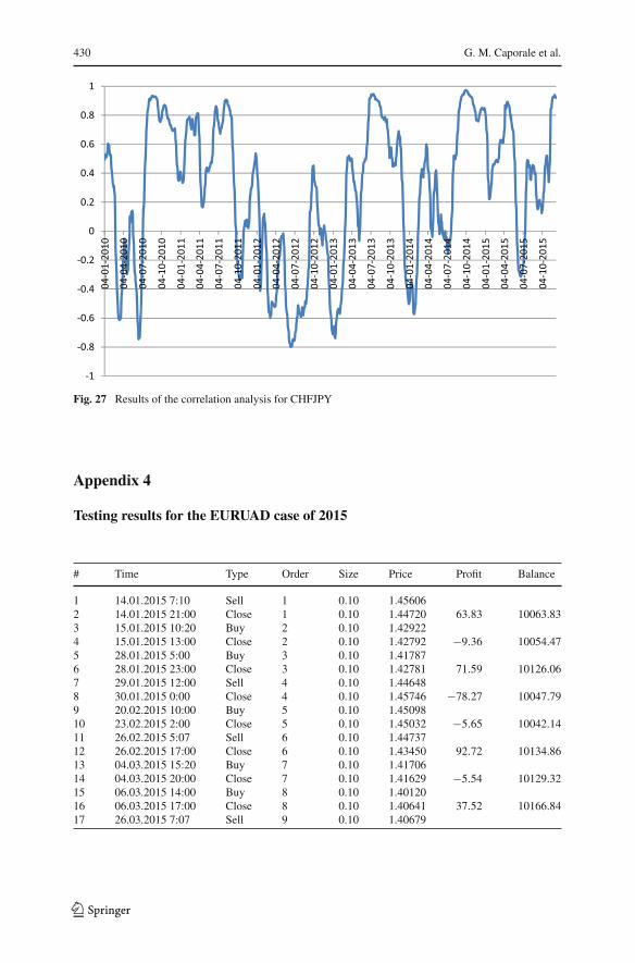
As a first step, we carry out simple correlation analysis. Values of the correla-tion coefficient >0.7 are defined as high correlation. Detailed results are presented inAppendix 3 Figs. 17–27. A summary is provided in Table 5.
As can be seen, the degree of correlation varies considerably across pairs. The fol-lowing analysis is carried out for the following ones: EURGBP, EURAUD, EURJPY,EURCHF, EURCAD, GBPAUD, GBPJPY, GBPCHF, AUDCAD, AUDJPY, CHFJPY.
The sample period for the obtaining the optimal parameters is 2010–2012. Out-of-the-sample testing is conducted for 2013, 2014 and 2015. The final testing of theoverall procedure is continuous testing for the 2010–2015 period.
For the optimisation procedure over the period 2010–2012 the slow correlation(based on daily data) equals 60 and the fast one 12 (based on hourly data). We usedthe slow correlation period 60 instead of 90 to obtain a bigger number of deals. Themain criterion to choose the best performer is total net profit (financial result of alltrades—it represents the difference between “Gross profit” and “Gross loss”), totaltrades (total amount of trade positions), profit factor (the ratio between total profit andtotal loss in per cents). A value of one implies that total profit is equal to total loss.The expected payoff is the average profit/loss factor of one trade. It also measures the
123
Searching for Inefficiencies in Exchange Rate Dynamics 419
Table 6 Optimisation results: period 2010–2012
Cross rate Optimal parameters* Results
Cor_day Cor_In Cor_Out Total profit Total trades Profit trades (%)
EURGBP 0.9 0.7 0.9 32 6 50
EURAUD 0.5 0.5 0.5 274 18 61
EURJPY 0.5 0.1 0.9 484 52 56
EURCHF 0.9 0.3 0.1 −25 13 54
EURCAD 0.6 0.2 0.1 388 64 66
GBPAUD 0.5 0.5 0.6 105 35 51
GBPJPY 0.6 0.4 0.6 570 35 60
GBPCHF 0.5 0.8 0.9 1196 14 64
AUDCAD 0.5 0.7 0.9 245 12 75
AUDJPY 0.6 0.7 0.9 609 20 70
CHFJPY 0.8 0.6 0.6 118 10 80
* Cor_day—daily correlation; Cor_In and Cor_Out—divergence and convergence criterions accordingly(based on hourly correlation)
expected profitability/unprofitability of the next trade and drawdown (the maximumdrawdown being related to the initial deposit).
The results of the optimisation procedure are presented in Table 6.As can be seen, the optimal parameters inmost cases generate profits. However, this
could be the result of data snooping, and therefore out-of-sample tests should be donebefore reaching any conclusions. The “optimal parameters” are used for out-of-sampletesting (2013, 2014, 2015). The results are presented in Table 7.
As can be seen, the results are rather unstable and confirm our suspicion of datasnooping affecting the optimization over the period 2010–2012. Nevertheless we alsoconduct the overall testing analysis (see Table 8).
The results are consistent with the previous ones, suggesting that data snoopingpossibly occurs in the case ofGBPCHF, EURJPY andAUDCAD.Therefore additionaltests are needed.
With the aim of establishing whether the trading results are statistically differentfrom the random trading ones we carry out t-tests. We chose this approach instead ofz-test because the sample size is less than 100. A t-test compares the means from twosamples to see whether they come from the same population. In our case the first isthe average profit/loss factor of one trade applying the trading strategy, and the secondis equal to zero because random trading (without transaction costs) should generatezero profit. In order to provide results which are closer to the real world we alsoincorporate the spread (as the biggest component of transaction costs) in the randomtrading results. This implies that the average profit per deal in random trading is not0, but equals the size of the spread.
The null hypothesis (H0) is that the mean is the same in both samples, and thealternative (H1) that it is not. The computed values of the t-test are compared with thecritical one at the 5 % significance level. Failure to reject H0 implies that there areno advantages from exploiting the trading strategy we test, whilst a rejection suggests
123
420 G. M. Caporale et al.
Table7
Out-of-sampletestingresults:p
eriods
2013
,201
4,20
15
Cross
rate
2013
2014
2015
Totalp
rofit
Totaltrades
Profi
ttrades(%
)To
talp
rofit
Totaltrades
Profi
ttrades(%
)To
talp
rofit
Totaltrades
Profi
ttrades(%
)
EURGBP
00
0−7
73
0−2
12
50
EURAUD
−205
956
−424
6744
327
59
EURJPY
−634
3037
325
2548
−310
2635
EURCHF
−51
40
03
67−1
637
43
EURCAD
326
67−4
4528
32−3
5235
46
GBPA
UD
−192
1735
−347
2232
461
2070
GBPJPY
−663
2945
−416
1650
−70
425
GBPC
HF
−456
30
−197
944
209
650
AUDCAD
−148
1155
−28
63−1
19
33
AUDJPY
−117
1338
414
1060
100
838
CHFJPY
346
5033
850
−225
633
123
Searching for Inefficiencies in Exchange Rate Dynamics 421
Table 8 Overall testing results:period 2010–2015
Cross rate Results
Total profit Total trades Profit trades (%)
EURGBP −60 11 36
EURAUD 503 78 62
EURJPY 339 133 50
EURCHF −213 27 48
EURCAD −193 135 54
GBPAUD 48 93 48
GBPJPY −133 82 54
GBPCHF 691 32 50
AUDCAD 81 40 58
AUDJPY 980 50 54
CHFJPY −50 30 53
Table 9 Example of t-test forthe EURAUD results in 2015
Parameter Value
Number of the trades 27
Total profit (points) 442.79
Average profit per trade (points) 16.39
Spread size (points) 5
Standard deviation (points) 46.49
t-test 2.39
t critical (0.95) 2.05
Null hypothesis Rejected
that a trading strategy focusing on the convergences/divergences in exchange ratedynamics can generate extra profits and therefore can be used to predict prices.
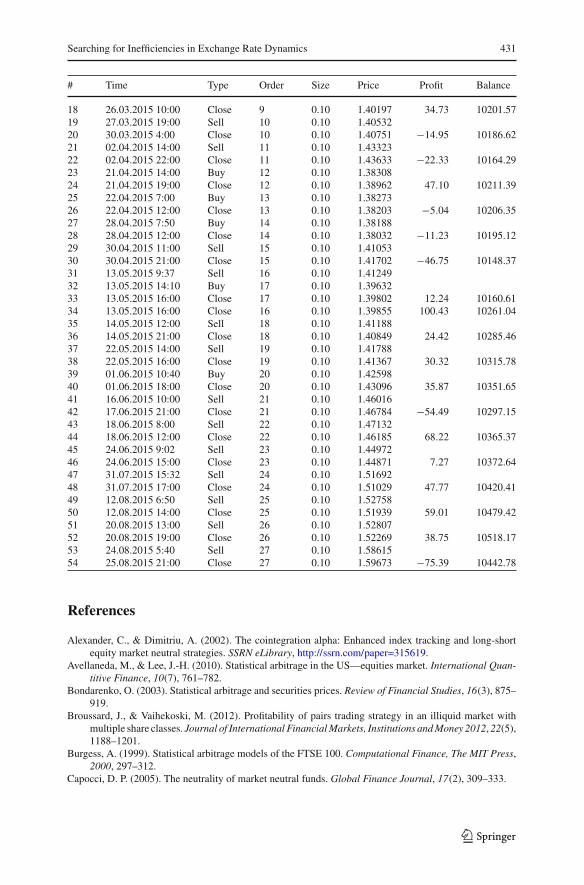
As an illustration, the complete trading results for the EURAUD in 2015 are pre-sented in Appendix 4. The t-test results are reported in Table 9.
Aswe can be seen,H0 is rejected,which implies that the trading results of EURAUDin 2015 are statistically different from the random ones and therefore the tradingstrategy is effective. The Overall testing results for the periods 2010–2012; 2013;2014; 2015; 2010–2015 are presented in Table 10.
Most of the trading results fail the test, i.e. they are not statistically different fromthe random ones, and therefore the trading strategy cannot beat the market. The twoexceptions are EURAUD and AUDJPY: in these two cases a trading strategy basedon the convergence/divergence indicator generates profits, providing at least someevidence in favour of its effectiveness.
Future research will consider extensions of the present analysis, namely the estima-tion of GARCH and stochastic volatility (SV) models, Kalman filtering etc. insteadof simple correlation analysis; the use of more sophisticated software for the test-ing procedures and programming the trading robots, such as Mathlab or R insteadof MetaTrader; refinements of the trading algorithm, checking for the absence of
daily correlation drop, incorporating “trend detection”, doing additional checks beforethe position opening; performing White’s Bootstrap Reality Check test and Hansen’sSuperior Predictive Ability test instead of simple t-tests and z-tests.
5 Conclusions
In this paper we develop a new approach to detecting inefficiencies in exchange ratedynamics based on double correlation analysis of financial asset dynamics. Dailycorrelations are taken to represent the “normal” behavior of asset prices, whilst hourlycorrelations are used to detect divergence/convergence and devise appropriate tradingstrategies.
The general rule is as follows: if the daily correlation between two assets is higherthan 0.5–0.7, they are considered to be diverging if their hourly correlation is lower than−0.5 and converging if it is higher than 0.5. On the basis of this rule we construct a newtechnical indicator (convergence/divergence indicator or CDI), which visualises bothtypes of correlation (daily and hourly) and provides the user with information aboutthe current state (divergence/convergence); divergence is defined as an inefficiencyin price movements. This indicator is shown to outperform other indicators of theoscillatory class and to generate profits (in the case of the EURAUD pair) withoutthe need for incorporating additional algorithms in the trading strategy. Testing of thetrading strategy based on CDI rules shows that in general it cannot beat the market.However, there a few exceptions (EURAUD and ADUJPY) providing at least someevidence supporting the profitability of such a trading strategy.
Open Access This article is distributed under the terms of the Creative Commons Attribution 4.0 Interna-tional License (http://creativecommons.org/licenses/by/4.0/), which permits unrestricted use, distribution,and reproduction in any medium, provided you give appropriate credit to the original author(s) and thesource, provide a link to the Creative Commons license, and indicate if changes were made.
Alexander, C., & Dimitriu, A. (2002). The cointegration alpha: Enhanced index tracking and long-shortequity market neutral strategies. SSRN eLibrary, http://ssrn.com/paper=315619.
Avellaneda, M., & Lee, J.-H. (2010). Statistical arbitrage in the US—equities market. International Quan-titive Finance, 10(7), 761–782.
Bondarenko, O. (2003). Statistical arbitrage and securities prices. Review of Financial Studies, 16(3), 875–919.
Broussard, J., & Vaihekoski, M. (2012). Profitability of pairs trading strategy in an illiquid market withmultiple share classes. Journal of International FinancialMarkets, Institutions andMoney 2012, 22(5),1188–1201.
Burgess, A. (1999). Statistical arbitrage models of the FTSE 100. Computational Finance, The MIT Press,2000, 297–312.
Capocci, D. P. (2005). The neutrality of market neutral funds. Global Finance Journal, 17(2), 309–333.
Chan, E. (2009). Quantitative trading: How to build your own algorithmic trading business. Hoboken, NJ:Wiley. 208 p.
Do, B., & Faff, R. (2010). Does simply pairs trading still work? Financial Analysts Journal, 66(4), 83–95.Dunis, C., & Ho, R. (2005). Cointegration portfolios of European equities for index tracking and market
neutral strategies. Journal of Asset Management, 6(1), 33–52.Dunis, C. L., & Shannon, G. (2005). Emerging markets of South-East and Central Asia: Do they still offer
a diversification benefit? Journal of Asset Management, 6(3), 168–190.Enders, W., & Granger, C. (1998). Unit-root tests and asymmetric adjustment with an example using the
term structure of interest rates. Journal of Business & Economic Statistics, 16(3), 304–311.Engle, R. F., & Granger, C. W. J. (1987). Co-integration and error correction: Representation, estimation,
and testing. Econometrica, 55(2), 251–276.Fama, E. F. (1970). Efficient markets: A review of theory and empirical work. Journal of Finance, 25(2),
383–417.Gatev, G., Goetzmann, N., & Rouwenhorst, K. (2006). Pairs trading: Performance of a relative value
arbitrage rule. Review of Financial Studies, 19(3), 797–827.Hogan, S., Jarrow, R., Teo, M., & Warchka, M. (2004). Testing market efficiency using statistical arbitrage
with applications to momentum and value strategies. Journal of Financial Economics, 73(3), 525–565.Hong, G., & Susmel, R. (2003). Pairs-trading in the Asian ADRMarket, Working Paper. http://www.bauer.
uh.edu/rsusmel/Academic/ptadr.pdf.Johansen, S. (1988). Statistical analysis of cointegration vectors. Journal of Economic Dynamics and Con-
trol, 12, 231–254.Khandani, A. E., & Lo, A. W. (2011). What happened to the quants in August 2007? Evidence from factors
and transactions data. Journal of Financial Markets, 14(1), 1–46.Lin,Y.-X.,Mccrae,M.,&Gulati, C. (2006). Loss protection in pairs trading throughminimumprofit bounds:
A cointegration approach. Journal of Applied Mathematics and Decision Sciences, 2006, 1–14.Nath, P. (2003). High frequency pairs trading with U.S. Treasury Securities: Risks and Rewards for Hedge
Funds. SSRN: http://ssrn.com/abstract=565441 or doi:10.2139/ssrn.565441.Perlin, M. (2009). Evaluation of pairs-trading strategy at the Brazilian financial market. Journal of Deriv-
atives & Hedge Funds, 15(2), 122–136.Plastun, A., & Kozmenko, S. (2011). Mutual influence of exchange assets: analysis and estimation. Banks
and Bank Systems; International Research Journal, No 2, 52–58.Vidyamurthy, G. (2004). Pairs trading, quantitative methods and analysis. Mississauga: Wiley. 224 p.Wilder, W. (1978). New concepts in technical trading systems. Pristine: Trend Research. 141 p.