72
. . . . . . Discrete-event-dynamic pump control Sebastian Roll & Heinz A Preisig Dept of Chemical Engineering NTNU, Trondheim Norway January 27, 2012

. . . . . .
Discrete-event-dynamic pump control
Sebastian Roll & Heinz A Preisig
Dept of Chemical EngineeringNTNU, Trondheim
Norway
January 27, 2012

. . . . . .
Contents
Project
DEDS Basics
Hybrid - automaton
Properties
Distillation pump control
. . . . . .
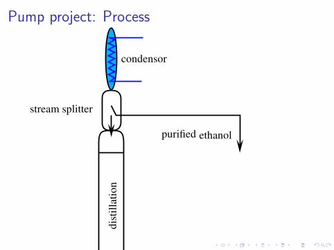
Pump project: Process
condensor
ethanol
waterboiler
dis
till
atio
n
purified
stream splitter

. . . . . .
Pump project: Process
ethanol
water
condensor
boiler
dis
till
atio
n
sensor tube
pump
purified
valve
b probe access

. . . . . .
Retrofit distillation
I Move condenser down and to the side
I Pump reflux back up to header
I Meter flux
I Provide sample point

. . . . . .
Retrofit distillation
I Move condenser down and to the side
I Pump reflux back up to header
I Meter flux
I Provide sample point

. . . . . .
Retrofit distillation
I Move condenser down and to the side
I Pump reflux back up to header
I Meter flux
I Provide sample point

. . . . . .
Retrofit distillation
I Move condenser down and to the side
I Pump reflux back up to header
I Meter flux
I Provide sample point

. . . . . .
Pump : peristaltic
I Volume transporter
I Calibrate →meter
I Kind control →accuracy

. . . . . .
Pump : peristaltic
I Volume transporter
I Calibrate →meter
I Kind control →accuracy

. . . . . .
Pump : peristaltic
I Volume transporter
I Calibrate →meter
I Kind control →accuracy

. . . . . .
Flow measurement: discretely observed volume
I Most instrumentation →expensive
I Discrete volume measure →cheap
I Provides average measure between two eventsI Event period not fixedI →PROCESS IS CLOCKI →depends on process dynamicsI →acceleration as uncertainty

. . . . . .
Flow measurement: discretely observed volume
I Most instrumentation →expensive
I Discrete volume measure →cheap
I Provides average measure between two eventsI Event period not fixedI →PROCESS IS CLOCKI →depends on process dynamicsI →acceleration as uncertainty

. . . . . .
Flow measurement: discretely observed volume
I Most instrumentation →expensive
I Discrete volume measure →cheapI Provides average measure between two events
I Event period not fixedI →PROCESS IS CLOCKI →depends on process dynamicsI →acceleration as uncertainty

. . . . . .
Flow measurement: discretely observed volume
I Most instrumentation →expensive
I Discrete volume measure →cheapI Provides average measure between two eventsI Event period not fixed
I →PROCESS IS CLOCKI →depends on process dynamicsI →acceleration as uncertainty

. . . . . .
Flow measurement: discretely observed volume
I Most instrumentation →expensive
I Discrete volume measure →cheapI Provides average measure between two eventsI Event period not fixedI →PROCESS IS CLOCK
I →depends on process dynamicsI →acceleration as uncertainty

. . . . . .
Flow measurement: discretely observed volume
I Most instrumentation →expensive
I Discrete volume measure →cheapI Provides average measure between two eventsI Event period not fixedI →PROCESS IS CLOCKI →depends on process dynamics
I →acceleration as uncertainty

. . . . . .
Flow measurement: discretely observed volume
I Most instrumentation →expensive
I Discrete volume measure →cheapI Provides average measure between two eventsI Event period not fixedI →PROCESS IS CLOCKI →depends on process dynamicsI →acceleration as uncertainty

. . . . . .
Pump project: Level glass

. . . . . .
Hybrid plant
plant quantizero-hold
discrete-event plant
u(k) u(t) x(t) x(k)
discrete-event input
continuous input signalcontinuous state
discrete-event state

. . . . . .
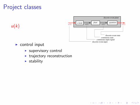
Project classes
plant quantizero-hold
discrete-event plant
u(k) u(t) x(t) x(k)
discrete-event input
continuous input signalcontinuous state
discrete-event state
u(k)
I control input
I supervisory controlI trajectory reconstructionI stability
I persistent fault
I fault detectionI fault isolationI fault counteraction supervisory controlI hazop analysis

. . . . . .
Project classes
plant quantizero-hold
discrete-event plant
u(k) u(t) x(t) x(k)
discrete-event input
continuous input signalcontinuous state
discrete-event state
u(k)
I control inputI supervisory control
I trajectory reconstructionI stability
I persistent fault
I fault detectionI fault isolationI fault counteraction supervisory controlI hazop analysis

. . . . . .
Project classes
plant quantizero-hold
discrete-event plant
u(k) u(t) x(t) x(k)
discrete-event input
continuous input signalcontinuous state
discrete-event state
u(k)
I control inputI supervisory controlI trajectory reconstruction
I stability
I persistent fault
I fault detectionI fault isolationI fault counteraction supervisory controlI hazop analysis
. . . . . .
Project classes
plant quantizero-hold
discrete-event plant
u(k) u(t) x(t) x(k)
discrete-event input
continuous input signalcontinuous state
discrete-event state
u(k)
I control inputI supervisory controlI trajectory reconstructionI stability
I persistent fault
I fault detectionI fault isolationI fault counteraction supervisory controlI hazop analysis

. . . . . .
Project classes
plant quantizero-hold
discrete-event plant
u(k) u(t) x(t) x(k)
discrete-event input
continuous input signalcontinuous state
discrete-event state
u(k)
I control inputI supervisory controlI trajectory reconstructionI stability
I persistent faultI fault detection
I fault isolationI fault counteraction supervisory controlI hazop analysis

. . . . . .
Project classes
plant quantizero-hold
discrete-event plant
u(k) u(t) x(t) x(k)
discrete-event input
continuous input signalcontinuous state
discrete-event state
u(k)
I control inputI supervisory controlI trajectory reconstructionI stability
I persistent faultI fault detectionI fault isolation
I fault counteraction supervisory controlI hazop analysis

. . . . . .
Project classes
plant quantizero-hold
discrete-event plant
u(k) u(t) x(t) x(k)
discrete-event input
continuous input signalcontinuous state
discrete-event state
u(k)
I control inputI supervisory controlI trajectory reconstructionI stability
I persistent faultI fault detectionI fault isolationI fault counteraction supervisory control
I hazop analysis

. . . . . .
Project classes
plant quantizero-hold
discrete-event plant
u(k) u(t) x(t) x(k)
discrete-event input
continuous input signalcontinuous state
discrete-event state
u(k)
I control inputI supervisory controlI trajectory reconstructionI stability
I persistent faultI fault detectionI fault isolationI fault counteraction supervisory controlI hazop analysis

. . . . . .
Discretising the state space 1
1. define state discretisation: vector of lists
2. yields discrete state space : a set of hypercubes
xa
xb
xc

. . . . . .
Discretising the state space 1
1. define state discretisation: vector of lists
2. yields discrete state space : a set of hypercubes
xa
xb
xc
. . . . . .
Discretising the state space 1
1. define state discretisation: vector of lists
2. yields discrete state space : a set of hypercubes
xa
xb
xc

. . . . . .
Discretising the state space 1
1. define state discretisation: vector of lists
2. yields discrete state space : a set of hypercubes
xa
xb
xc

. . . . . .
Event
.Event definition..
......
An event is defined as the crossing of a boundary surface of adiscrete state hypercube. The boundary itself is dynamicallyallocated, that the boundary point itself belongs to the statefrom which one enters the boundary. In case the trajectoryfollows the boundary for a piece of the way, it is the exit pointthat determines the state transition.

. . . . . .
Discretising the state space 2
xa
xb
xc
xc = 0
0 = fc(xa, xb, xc)
a stencil
direction of gradient in xc

. . . . . .
Model system

. . . . . .
The trajectories

. . . . . .
The discrete state space

. . . . . .
The zero surfaces - here lines

. . . . . .
The directions of change
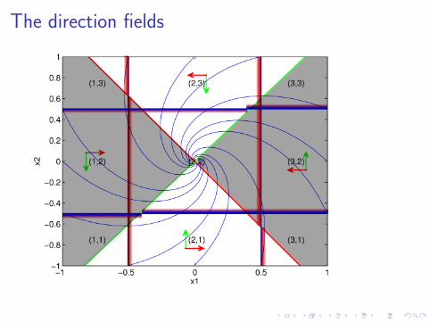
. . . . . .
The direction fields

. . . . . .
The directions

. . . . . .
Automaton table/graph
I adjacency matrix or
I state transition matrix
I output matrix

. . . . . .
Automaton table/graph
change in x1 change in x2state -1 1 -1 11,1 1,21,2 2,2 1,31,3 2,32,1 1,1 2,22,2 1,2 3,2 2,1 2,32,3 3,3 2,23,1 2,13,2 2,2 3,13,3 3,2
next state

. . . . . .
Stability ???
I circle
I converging
I diverging
I Liapunov function in continuous domain: ellipse
I Discrete: if having made a circle inside a boxsystem stays in the box.

. . . . . .
Does it work for more complex systems ?

. . . . . .
Applications
I Fault detection / isolation with K W Lim, NUS(Singapore)
I Supervisory control with Lunze TUHH (Hamburg) nowBochum: application Bosch carburettor control
I Student experiment (coffee machine ETH, washingmachine UNSW, saft machine (TUE, NTNU))
I Pump control (NTNU)

. . . . . .
Applications
I Fault detection / isolation with K W Lim, NUS(Singapore)
I Supervisory control with Lunze TUHH (Hamburg) nowBochum: application Bosch carburettor control
I Student experiment (coffee machine ETH, washingmachine UNSW, saft machine (TUE, NTNU))
I Pump control (NTNU)

. . . . . .
Applications
I Fault detection / isolation with K W Lim, NUS(Singapore)
I Supervisory control with Lunze TUHH (Hamburg) nowBochum: application Bosch carburettor control
I Student experiment (coffee machine ETH, washingmachine UNSW, saft machine (TUE, NTNU))
I Pump control (NTNU)

. . . . . .
Applications
I Fault detection / isolation with K W Lim, NUS(Singapore)
I Supervisory control with Lunze TUHH (Hamburg) nowBochum: application Bosch carburettor control
I Student experiment (coffee machine ETH, washingmachine UNSW, saft machine (TUE, NTNU))
I Pump control (NTNU)

. . . . . .
Pump project: Process
ethanol
water
condensor
boiler
dis
till
atio
n
sensor tube
pump
purified
valve
b probe access
. . . . . .
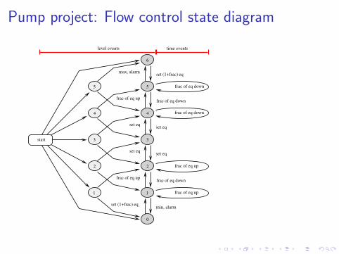
Pump project: Flow control state diagram
5
4
3
2
1
6
0
5
4
3
2
1
max, alarm
frac of eq up
frac of eq up
set (1+frac) eq
set (1+frac) eqmin, alarm
frac of eq down
frac of eq down
set eqset eq
set eqset eq
frac of eq down
frac of eq down
frac of eq up
frac of eq up
start
level events time events

. . . . . .
I First level event: do nothing
I All level events after first:
Vk := Vposition
tk := tevent
I all level events after second:
∆tk := tk − tk−1
∆V :=Vk − Vk−1
∆tk
Vc := Vp +∆V

. . . . . .
Pump project: Calibration supervisory control state
diagram
fill
callibrate
end
start
set min speed
set overfill timer
start pump
close feed valve
overfill timer
take time, volume, speed
level 6,5,4,3,2,1
level 0
compute flow rates
increment speed
level 6
speed > max
open feed valve
open feed valve

. . . . . .
Pump project: Calibration results

. . . . . .
Conclusion DEDS modelling
I analysis is based on system’s vector field
I component-wise analysis
I limits scopeI thus dimensionI local automata
I local refinement is possible
I property: deterministic continuous system →non-deterministic automaton
I property: Liapunov functions can be discretised too

. . . . . .
Conclusion DEDS modelling
I analysis is based on system’s vector field
I component-wise analysisI limits scope
I thus dimensionI local automata
I local refinement is possible
I property: deterministic continuous system →non-deterministic automaton
I property: Liapunov functions can be discretised too

. . . . . .
Conclusion DEDS modelling
I analysis is based on system’s vector field
I component-wise analysisI limits scopeI thus dimension
I local automata
I local refinement is possible
I property: deterministic continuous system →non-deterministic automaton
I property: Liapunov functions can be discretised too

. . . . . .
Conclusion DEDS modelling
I analysis is based on system’s vector field
I component-wise analysisI limits scopeI thus dimensionI local automata
I local refinement is possible
I property: deterministic continuous system →non-deterministic automaton
I property: Liapunov functions can be discretised too

. . . . . .
Conclusions: pump control
I Works fine
I Cheap
I Adapts to dynamics ←nature of DEDS

. . . . . .
Conclusions: pump control
I Works fine
I Cheap
I Adapts to dynamics ←nature of DEDS

. . . . . .
Conclusions: pump control
I Works fine
I Cheap
I Adapts to dynamics ←nature of DEDS

. . . . . .
Conclusions: issues
I Volume measurement is dead volume
I →periodic emptying
I →reduce volume
I →compromise accuracy vs refreshing hold-up

. . . . . .
Conclusions: issues
I Volume measurement is dead volume
I →periodic emptying
I →reduce volume
I →compromise accuracy vs refreshing hold-up

. . . . . .
Conclusions: issues
I Volume measurement is dead volume
I →periodic emptying
I →reduce volume
I →compromise accuracy vs refreshing hold-up

. . . . . .
Conclusions: issues
I Volume measurement is dead volume
I →periodic emptying
I →reduce volume
I →compromise accuracy vs refreshing hold-up

. . . . . .
End
Questions ?


