SeborgCSTR basics - openmodelica.org · Modelica code for original Seborg et al model...

SeborgCSTR_basics

March 13, 2018

1 Use of Modelica + Python in Process Systems Engineering Education

1.1 Basic analysis of “Seborg reactor”

1.1.1 Bernt Lie

1.1.2 University College of Southeast Norway

Basic import and definitions

In [1]: from OMPython import ModelicaSystem

import numpy as np

import numpy.random as nr

%matplotlib inline

import matplotlib.pyplot as plt

import pandas as pd

LW1 = 2.5

LW2 = LW1/2

Cb1 = (0.3,0.3,1)

Cb2 = (0.7,0.7,1)

Cg1 = (0,0.6,0)

Cg2 = (0.5,0.8,0.5)

Cr1 = "Red"

Cr2 = (1,0.5,0.5)

LS1 = "solid"

LS2 = "dotted"

LS3 = "dashed"

figpath = "../figs/"

1.1.3 Nonlinear reactor model from Seborg et al.

Process diagram

Original state space model We consider the original Seborg et al. model, written as:

dcA

dt=

V̇i

V(cA,i − cA)− a · r

1

CpdTdt

=V̇i

VCp,i (Ti − T) +

(−∆rH̃

)rV + Q̇

Here:

r = kcaA

k = k0 exp(− E

RT

)Q̇ = UA (Tc − T)

In the original Seborg et al. model, a = 1, while ∆r is constant, V̇e = V̇i, and Cp = Cp,i isconstant.

Modelica code for original Seborg et al model “ModSeborgCSTRorg” within package “Se-borgCSTR”

model ModSeborgCSTRorg

// Model of ORiGinal Seborg CSTR in ode form

// author: Bernt Lie

// University of Southeast Norway

// November 7, 2017

//

// Parameters

parameter Real V = 100 "Reactor volume, L";

parameter Real rho = 1e3 "Liquid density, g/L";

parameter Real a = 1 "Stoichiometric constant, -";

parameter Real EdR = 8750 "Activation temperature, K";

parameter Real k0 = exp(EdR/350) "Pre-exponential factor, 1/min";

parameter Real cph = 0.239 "Specific heat capacity of mixture, J.g-1.K-1";

parameter Real DrHt = -5e4 "Molar enthalpy of reaction, J/mol";

parameter Real UA = 5e4 "Heat transfer parameter, J/(min.K)";

// Initial state parameters

parameter Real cA0 = 0.5 "Initial concentration of A, mol/L";

parameter Real T0 = 350 "Initial temperature, K";

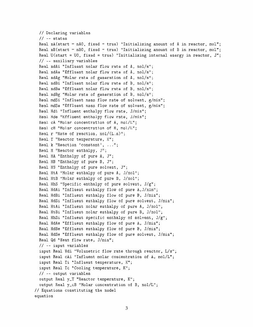
// Declaring variables

// -- states

Real cA(start = cA0, fixed = true) "Initializing concentration of A in reactor, mol/L";

Real T(start = T0, fixed = true) "Initializing temperature in reactor, K";

// -- auxiliary variables

Real r "Rate of reaction, mol/(L.s)";

Real k "Reaction 'constant', ...";

Real Qd "Heat flow rate, J/min";

// -- input variables

input Real Vdi "Volumetric flow rate through reactor, L/min";

input Real cAi "Influent molar concentration of A, mol/L";

2

input Real Ti "Influent temperature, K";

input Real Tc "Cooling temperature', K";

// -- output variables

output Real y_T "Reactor temperature, K";

// Equations constituting the model

equation

// Differential equations

der(cA) = Vdi*(cAi-cA)/V- a*r;

der(T) = Vdi*(Ti-T)/V + (-DrHt)*r/(rho*cph) + Qd/(rho*V*cph);

// Algebraic equations

r = k*cAâ;

k = k0*exp(-EdR/T);

Qd = UA*(Tc-T);

// Outputs

y_T = T;

end ModSeborgCSTRorg;

1.1.4 Nominal model study

Instantiating model

In [2]: sr_org = ModelicaSystem("SeborgCSTR.mo","SeborgCSTR.ModSeborgCSTRorg")

2018-03-13 14:45:03,198 - OMPython - INFO - OMC Server is up and running at file:///c:/users/bernt_~1/appdata/local/temp/openmodelica.port.7aeb88afd36e4ddcac9a04160acc3f3b

Checking quantity names for model

In [3]: pd.DataFrame(sr_org.getQuantities())

Out[3]: Changeable Description Name \

0 false Initializing temperature in reactor, K T

1 false Initializing concentration of A in reactor, mol/L cA

2 false der(Initializing temperature in reactor, K) der(T)

3 false der(Initializing concentration of A in reactor... der(cA)

4 false None $cse1

5 false Heat flow rate, J/min Qd

6 true Cooling temperature', K Tc

7 true Influent temperature, K Ti

8 true Volumetric flow rate through reactor, L/min Vdi

9 true Influent molar concentration of A, mol/L cAi

10 false Reaction 'constant', ... k

11 false Rate of reaction, mol/(L.s) r

12 false Reactor temperature, K y_T

13 true Molar enthalpy of reaction, J/mol DrHt

14 true Activation temperature, K EdR

15 true Initial temperature, K T0

16 true Heat transfer parameter, J/(min.K) UA

17 true Reactor volume, L V

3

18 true Stoichiometric constant, - a

19 true Initial concentration of A, mol/L cA0

20 true Specific heat capacity of mixture, J.g-1.K-1 cph

21 false Pre-exponential factor, 1/min k0

22 true Liquid density, g/L rho

Value Variability alias aliasvariable

0 None continuous noAlias None













13 -50000.0 parameter noAlias None

14 8750.0 parameter noAlias None







21 None parameter noAlias None


Observe the artifically named variable “$cse1” this is a variable that the system has created,and is not found in the underlying Modelica code.

Setting simulation length

In [4]: sr_org.getSimulationOptions()

Out[4]: {'solver': 'dassl',

'startTime': 0.0,

'stepSize': 0.002,

'stopTime': 1.0,

'tolerance': 1e-06}

In [5]: sr_org.setSimulationOptions(stopTime=15,stepSize=0.05)

Checking input

In [6]: u = sr_org.getInputs()

4

In [7]: u

Out[7]: {'Tc': None, 'Ti': None, 'Vdi': None, 'cAi': None}

In [8]: u.keys()

Out[8]: ['Vdi', 'cAi', 'Tc', 'Ti']

In [9]: u.values()

Out[9]: [None, None, None, None]

Setting nominal inputs

In [10]: sr_org.setInputs(Tc=300)

sr_org.setInputs(Ti=350)

sr_org.setInputs(Vdi=100)

sr_org.setInputs(cAi=1)

In [11]: u = sr_org.getInputs()

u.keys()

Out[11]: ['Vdi', 'cAi', 'Tc', 'Ti']

In [12]: u["Ti"]

Out[12]: [(0.0, 350), (15.0, 350)]

Simulating system for three cases of inputs, and extracting results


sr_org.simulate()

tm_org0, T_org0, Tc_org0, cA_org0 = sr_org.getSolutions("time","T","Tc","cA")

sr_org.setInputs(Tc=300+5)

sr_org.simulate()

tm_org0p, T_org0p, Tc_org0p, cA_org0p = sr_org.getSolutions("time","T","Tc","cA")

sr_org.setInputs(Tc=300-10)

sr_org.simulate()

tm_org0m, T_org0m, Tc_org0m, cA_org0m = sr_org.getSolutions("time","T","Tc","cA")

Plotting results

In [14]: plt.plot(tm_org0,T_org0-273.15,LW=LW1,color=Cg1,label=r"$T_{\mathrm{c,org}}^{\ast}$")

plt.plot(tm_org0p,T_org0p-273.15,LW=LW1,color=Cr1,label=r"$T_{\mathrm{c,org}}^{\ast}+5$")

plt.plot(tm_org0m,T_org0m-273.15,LW=LW1,color=Cb1,label=r"$T_{\mathrm{c,org}}^{\ast}-10$")

plt.legend(ncol=3)

plt.title("Reactor temperature")

plt.xlabel(r"time $t$ [min]")

plt.ylabel(r"$T$ [${}^\circ \mathrm{C}$]")

plt.grid()

plt.xlim(0,15)

figfile = "tempSeborgCSTRorg.pdf"

plt.savefig(figpath+figfile)

5

In [15]: plt.plot(tm_org0,cA_org0,LW=LW1,color=Cg1,label=r"$T_{\mathrm{c,org}}^{\ast}$")

plt.plot(tm_org0p,cA_org0p,LW=LW1,color=Cr1,label=r"$T_{\mathrm{c,org}}^{\ast}+5$")

plt.plot(tm_org0m,cA_org0m,LW=LW1,color=Cb1,label=r"$T_{\mathrm{c,org}}^{\ast}-10$")

plt.legend(ncol=3,loc=7)

plt.title("Concentration of $\mathrm{A}$")


plt.ylabel(r"$c_{\mathrm{A}}$ [mol/L]")

plt.grid()

plt.xlim(0,15)

figfile = "concSeborgCSTRorg.pdf"


6

In [16]: plt.plot(tm_org0,Tc_org0-273.15,LW=LW1, color=Cg1, label=r"$T_\mathrm{c}^{\ast}$")

plt.plot(tm_org0p,Tc_org0p-273.15,LW=LW1,color=Cr1, label=r"$T_\mathrm{c}^{\ast}+5$")

plt.plot(tm_org0m,Tc_org0m-273.15,LW=LW1,color=Cb1, label=r"$T_\mathrm{c}^{\ast}-10$")

plt.title("Cooling liquid temperature")


plt.ylabel(r"$T_\mathrm{c}$ [${}^\circ \mathrm{C}$]")

plt.grid()

plt.axis(ymin=15,ymax=35)

plt.xlim(0,15)


figfile = "coolSeborgCSTRorg.pdf"


7

1.1.5 Analysis: why oscillations?

Steady state model: steady concentration gives

dcA

dt= 0 ⇒ 0 =

V̇i

V(cA,i − cA)− kcA ⇒ cA(T) =

V̇i/V

k0 exp(− E/R

T

)+ V̇i/V

cA,i

while steady temperature gives

CpdTdt

= 0 ⇒ 0 =V̇i

VCp (Ti − T) +

(−∆rH̃

)rV + Q̇ ⇒

0 =V̇i

VCp (Ti − T) + UA (Tc − T)︸︷︷︸

=−Q̇rm(T)

+(−∆rH̃

)k0 exp

(−E/R

T

)cA(T) · V︸︷︷︸

=Q̇gen(T)

We now plot “removed heat rate” Q̇rm(T) and “generated heat rate” Q̇gen(T): at equilibrium,they must be equal.

In [17]: EdR = 8750

k0 = np.exp(EdR/350)

VdidV = 1

cAi = 1

def cA(T):

8

return VdidV/(k0*np.exp(-EdR/T) + VdidV)*cAi

#

rho = 1e3

V = 100

cph = 0.239

Cp = rho*V*cph

DrHt = -5e4

UA = 5e4

Ti = 350

Tc = 300

def Qdrm(T,Tc):

return -(VdidV*Cp*(Ti-T) + UA*(Tc-T))

def Qdgen(T):

return (-DrHt)*k0*np.exp(-EdR/T)*cA(T)*V

In [18]: TT = np.linspace(50,100)

plt.plot(TT, Qdgen(TT+273.15)/1e6,LW=LW1, color=Cr1, label=r"$\dot{Q}_\mathrm{gen}$")

plt.plot(TT, Qdrm(TT+273.15,Tc)/1e6,LW=LW1, color=Cb1, label=r"$\dot{Q}_\mathrm{rm}$")

plt.plot((350-273.15)*np.array([1,1]), [0,5],LW=LW1,color=Cg1,LS=LS2)

plt.plot([50,100], Qdrm(350,Tc)/1e6*np.array([1,1]),LW=LW1,color=Cg1,LS=LS2)

plt.plot((50.8)*np.array([1,1]), [0,5],LW=LW2,color=Cg2,LS=LS2)

plt.plot([50,100], Qdrm(50.8+273.15,Tc)/1e6*np.array([1,1]),LW=LW2,color=Cg2,LS=LS2)

plt.plot((97.2)*np.array([1,1]), [0,5],LW=LW2,color=Cg2,LS=LS2)


plt.title("Generated vs. removed heat rates")

plt.xlabel(r"temperature $T$ [C]")

plt.ylabel(r"$\dot{Q}$ [MJ/min]")

plt.grid()

plt.xlim(50,100)

plt.ylim(np.min(Qdrm(TT+273.15,Tc)/1e6), np.max(Qdrm(TT+273.15,Tc)/1e6))

plt.legend()

figfile = "equilSeborgCSTRorg.pdf"


9

Observe that the system has 3 equilibrium points. For the Seborg reactor, we start the systemat T = 350 − 273.15 [C], which is at the intersection of the thick green, dotted lines. If the reactoris operated so that the temperature becomes higher than 350 − 273.15 [C], a higher heat rate isgenerated than removed, and the temperature increases. If, on the other hand, the temperatureis operated so that the temperature becomes lower than 350 − 273.15 [C], then the removal heatrate is higher than the generated heat rate, and the reactor is cooled. In summary: the equilibriumpoint given by the green cross is unstable. Similar arguments leads to the conclusion that the othertwo equilibrium points (at ca. T = 50.8 [C] and ca. T = 97.2 [C]) are stable. This analysis doesnot explain oscillations, but it seems reasonable that oscillations may occur: * If the temperatureincreases, generated heat rate (Q̇gen) will first increase. However, concentration of species A dropsand eventually the reaction rate will draw to a halt - and generated heat rate will drop. Thus, thereactor temperature will drop. * As the reactor cools down, species A will increase in concentrationdue to addition of fresh A in the influent. Then, eventually, the reaction rate will “ignite” again,and the generated heat rate will again increase, leading to increasing temperature. * This will takeplace cyclically.



plt.plot(TT, Qdrm(TT+273.15,Tc)/1e6,LW=LW2, color="blue", LS = LS2, label=r"$\dot{Q}_\mathrm{rm}$, $T_\mathrm{c}$")

plt.plot(TT, Qdrm(TT+273.15,Tc+5)/1e6,LW=LW1, color=Cb2, label=r"$\dot{Q}_\mathrm{rm}$, $T_\mathrm{c}+5$")

plt.plot(TT, Qdrm(TT+273.15,Tc-10)/1e6,LW=LW1, color=Cb1, label=r"$\dot{Q}_\mathrm{rm}$, $T_\mathrm{c}-10$")

#

plt.plot((350-273.15)*np.array([1,1]), [-1,6],LW=LW1,color=Cg1,LS=LS2)

plt.plot([30,110], Qdrm(350,Tc)/1e6*np.array([1,1]),LW=LW1,color=Cg1,LS=LS2)

10

plt.plot((50.8)*np.array([1,1]), [-1,6],LW=LW2,color=Cg2,LS=LS2)




#




plt.grid()

plt.xlim(35,110)

plt.ylim(np.min(Qdrm(TT+273.15,Tc+5)/1e6), np.max(Qdrm(TT+273.15,Tc-10)/1e6))

plt.legend()

figfile = "equil_1_SeborgCSTRorg.pdf"


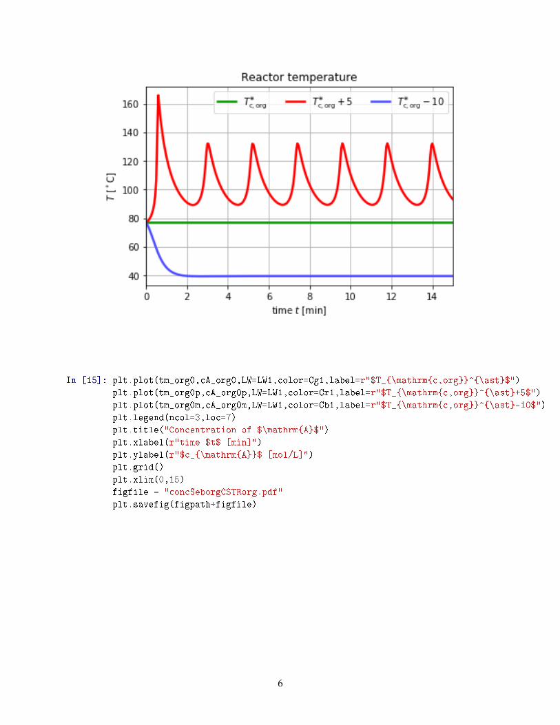
Observe that for cooling temperature Tc − 10, the initial temperature leads to reduced temper-ature until the single equilibrium point at ca. Tc = 40 [C] is reached. For the warmer cooling tem-perature (= less cooling) of Tc + 5, the initial temperature leads to increased temperature. Whileit may seem like there is a single, stable equilibrium at ca. Tc = 103 [C] (and possibly a pointwhich is difficult to interpret at ca. Tc = [60, 65] [C], it is important to realize that this analysis ispurely based on steady state analysis, and that the dynamics may (and: in fact does!) influencethe behavior.

11

1.1.6 Time varying inputs

In [20]: uTc = [(0,300),(2,300),(2,300-10),(5,300-10),(5,300),(7,300),(7,300+5),(30,300+5)]

uTi = [(0,350),(15,350),(15,340),(20,340),(20,360),(30,360)]

In [21]: sr_org.setInputs(Tc=uTc)

sr_org.setInputs(Ti=uTi)

In [22]: sr_org.setSimulationOptions(stopTime=30)

sr_org.simulate()

In [23]: tm, T, Tc, Ti = sr_org.getSolutions("time","T","Tc","Ti")

plt.plot(tm,Tc-273.15,LW=LW1,color=Cg1,label=r"$T_{\mathrm{c}}$")

plt.plot(tm,Ti-273.15,LW=LW1,color=Cb1,label=r"$T_{\mathrm{i}}$")

plt.plot(tm,T-273.15,LW=LW1,color=Cr1,label=r"$T$")

plt.title("Temperatures, original model")



plt.grid()

plt.xlim(0,30)

plt.legend()

figfile = "varInputSeborgCSTRorg.pdf"


12

SeborgCSTR_control_basic

March 13, 2018


1.1 Basic control of “Seborg reactor”

1.1.1 Bernt Lie




import numpy as np


%matplotlib inline


import pandas as pd

LW1 = 2.5

LW2 = LW1/2

Cb1 = (0.3,0.3,1)

Cb2 = (0.7,0.7,1)

Cg1 = (0,0.6,0)

Cg2 = (0.5,0.8,0.5)

Cr1 = "Red"

Cr2 = (1,0.5,0.5)

LS1 = "solid"

LS2 = "dotted"

LS3 = "dashed"


1.1.3 Basic control design

Instantiating models and setting inputs


2018-03-13 16:09:31,720 - OMPython - INFO - OMC Server is up and running at file:///c:/users/bernt_~1/appdata/local/temp/openmodelica.port.8ef95b56c9d44764834290989a4a104e

1

In [3]: sr_org.setSimulationOptions(stopTime=15,stepSize=0.05)

#

sr_org.setInputs(Tc=300)




Linearizing model

In [4]: sr_org.getLinearizationOptions()

Out[4]: {'numberOfIntervals': 500.0,

'startTime': 0.0,

'stepSize': 0.002,

'stopTime': 1.0,

'tolerance': 1e-08}

In [5]: A_org, B_org, C_org, D_org = sr_org.linearize()

2018-03-13 16:09:39,717 - OMPython - INFO - OMC Server is up and running at file:///c:/users/bernt_~1/appdata/local/temp/openmodelica.port.13c75508c0b947d79baae3689c8f328c

In [6]: A_org

Out[6]: array([[ 4.37955768e+00, 2.09205021e+02],

[ -3.57142857e-02, -2.00000000e+00]])

In [7]: B_org

Out[7]: array([[ 2.09205021e+00, 1.00000000e+00, 1.70530257e-15,

0.00000000e+00],

[ 0.00000000e+00, 0.00000000e+00, 5.00000000e-03,

1.00000000e+00]])

In [8]: C_org

Out[8]: array([[ 1., 0.]])

In [9]: D_org

Out[9]: array([[ 0., 0., 0., 0.]])

In [10]: sr_org.getLinearInputs()

Out[10]: ['Tc', 'Ti', 'Vdi', 'cAi']

In [11]: sr_org.getLinearStates()

Out[11]: ['T', 'cA']

In [12]: sr_org.getLinearOutputs()

Out[12]: ['y_T']

2

Theoretical results With x = (T, nA), u = (Tc,i, Ti, V̇, cA,i) and y = cA, the linearized model is:

dxδ

dt= Axδ + Buδ

yδ = Cxδ + Duδ

where:

A =

(4.3796 2.0921−3.5714 −2

)

B =

(2.0921 1 0 0

0 0 0.5 100

)

C =(

0 0.01)

D =(

0 0 0 0)

This means that OMPython/the Python API has correctly linearized the model.

In [13]: np.linalg.eig(A_org)

Out[13]: (array([ 2.83388381, -0.45432613]), array([[ 0.99997271, -0.99973316],

[-0.00738812, 0.0230998 ]]))

Transfer function from Tc to T (from MATLAB due to some lack of support for control toolboxin Python):

Observe. . . At the initial state, the system is open loop unstable due to the eigenvalue at+2.83388381. Observe also that with Tc as the control input/manipulatable variable and T as thecontrolled output, the system has a zero at 2.092 · s + 4.184 = 0 ⇒ s = −2; in other words, thezero dynamics is stable!

Tuning P-controller A P-controller for controlling output y = T via control input u = Tc willhave form u = T∗

c + Kp(Tref − T). This will change the expression for Q̇rm to:

−Q̇rm =V̇i

VCp (Ti − T) + UA

(T∗

c + Kp(Tref − T)− T)

In [14]: EdR = 8750

k0 = np.exp(EdR/350)

VdidV = 1

cAi = 1

def cA(T):

return VdidV/(k0*np.exp(-EdR/T) + VdidV)*cAi

#

3

rho = 1e3

V = 100

cph = 0.239

Cp = rho*V*cph

DrHt = -5e4

UA = 5e4

Ti = 350

Tcast = 300

Tref = 350

Kp = 0

def Qdrm(T,Kp):

return -(VdidV*Cp*(Ti-T) + UA*(Tcast+Kp*(Tref-T)-T))

def Qdgen(T):

return (-DrHt)*k0*np.exp(-EdR/T)*cA(T)*V



plt.plot(TT, Qdrm(TT+273.15,Kp)/1e6,LW=LW1, color=Cb1, label=r"$\dot{Q}_\mathrm{rm}$, $K_\mathrm{p} = 0$")

plt.plot(TT, Qdrm(TT+273.15,1)/1e6,LW=LW1, color=Cb2, label=r"$\dot{Q}_\mathrm{rm}$, $K_\mathrm{p} = 1$")

plt.plot(TT, Qdrm(TT+273.15,3)/1e6,LW=LW1, color=Cb2, LS = LS2, label=r"$\dot{Q}_\mathrm{rm}$, $K_\mathrm{p} = 3$")


#


plt.plot([30,110], Qdrm(350,Kp)/1e6*np.array([1,1]),LW=LW1,color=Cg1,LS=LS2)


plt.plot([30,110], Qdrm(50.8+273.15,Kp)/1e6*np.array([1,1]),LW=LW2,color=Cg2,LS=LS2)



#




plt.grid()

plt.xlim(35,110)

plt.ylim(np.min(Qdrm(TT+273.15,Kp)/1e6), np.max(Qdrm(TT+273.15,Kp)/1e6))

plt.legend()

figfile = "equil_controlled_SeborgCSTRorg.pdf"


4

In [16]: plt.plot(TT, Qdgen(TT+273.15)/1e6,LW=LW1, color=Cr1, label=r"$\dot{Q}_\mathrm{gen}$")

plt.plot(TT, Qdrm(TT+273.15,Kp)/1e6,LW=LW1, color=Cb1, label=r"$\dot{Q}_\mathrm{rm}$, $K_\mathrm{p} = 0$")

plt.plot(TT, Qdrm(TT+273.15,1)/1e6,LW=LW1, color=Cb2, label=r"$\dot{Q}_\mathrm{rm}$, $K_\mathrm{p} = 1$")



#


plt.plot([30,110], Qdrm(350,Kp)/1e6*np.array([1,1]),LW=LW1,color=Cg1,LS=LS2)





#




plt.grid()

plt.xlim(76,78)

plt.ylim(2.2,2.8)

plt.legend()

figfile = "equil_detail_controlled_SeborgCSTRorg.pdf"


5

Observe. . . With Kp = 0, we have seen that the system is (open loop) unstable. With Kp = 1,the system appears to have a stable equilibrium point, and the larger the value for the gain is, thelarger the stability margin becomes. (This is contrary to open-loop stable systems.) However, aswe will see below: the choice Kp = 1 is not sufficient go guarantee stability: we need to considerboth the effect in temperature and in concentration!

Root locus diagram for system with P-controller

In [17]: A_ol = A_org

B_ol = np.zeros((A_ol.shape[0],1))

B_ol[:,0] = B_org[:,0]

C_ol = C_org

#

KKp = np.linspace(-1,1.2)

Eig = np.zeros((KKp.size,2),np.dtype(complex))

#

for (i,Kp) in enumerate(KKp):

A_cl = A_org - Kp*B_ol*C_ol

Eig[i,:] = np.linalg.eig(A_cl)[0]

#

plt.plot(np.real(Eig)[:,0],np.imag(Eig)[:,0],"x",color=Cr1,markersize=5)

plt.plot(np.real(Eig)[:,1],np.imag(Eig)[:,1],"x",color=Cr1,markersize=5, label=r"$K_\mathrm{p} < 1.2$")

#

6

KKp = np.linspace(1.2,8)

Eig = np.zeros((KKp.size,2),np.dtype(complex))

#

for (i,Kp) in enumerate(KKp):

A_cl = A_org - Kp*B_ol*C_ol

Eig[i,:] = np.linalg.eig(A_cl)[0]

#

plt.plot(np.real(Eig)[:,0],np.imag(Eig)[:,0],"+",color=Cb1,markersize=5)

plt.plot(np.real(Eig)[:,1],np.imag(Eig)[:,1],"+",color=Cb1,markersize=5, label=r"$K_\mathrm{p} > 1.2$")

#

Eig0 = np.linalg.eig(A_ol)[0]

plt.plot(np.real(Eig0)[0],np.imag(Eig0)[0],"x",color=Cg1,markersize=8)

plt.plot(np.real(Eig0)[1],np.imag(Eig0)[1],"x",color=Cg1,markersize=8, label=r"$K_\mathrm{p} = 0$")

#

Eig1 = np.linalg.eig(A_org - 5.7*B_ol*C_ol)[0]

plt.plot(np.real(Eig1)[0],np.imag(Eig1)[0],"o",color=Cg1,markersize=8)

plt.plot(np.real(Eig1)[1],np.imag(Eig1)[1],"o",color=Cg1,markersize=8, label=r"$K_\mathrm{p} = 5.7$")

#

plt.grid()

plt.xlabel(r"$\Re [ \lambda (A_\mathrm{cl}) ]$")

plt.ylabel(r"$\Im [ \lambda (A_\mathrm{cl}) ]$")

plt.title(r"Closed loop eigenvalues as a function of $K_\mathrm{p}\in\{-1,8\}$")

plt.legend()

figfile = "ClosedLoop_Eigenvals_SeborgCSTRorg.pdf"


7

Observe. . . The system appears to be stable with a P-controller when Kp > 1.2 or so. WithKp ≈ 5.7, both eigenvalues become real with similar values. Some modification may be needed ifwe add integral action, but probably not much. We could probably choose Ti ∈ {2, 5} or so (some10 times closed loop timeconstant of ca. 1/5).

1.1.4 Simulation of system with P-controller

Modelica model for PI control system

model PIconSeborgCSTRorg

// Simulation of Seborg Reactor



// January 10, 2018

//

// Instantiate model of Seborg Reactor (sr)

ModSeborgCSTRorg srORG;

// Declaring parameters

parameter Real Kp = 0 "Proportional gain in P-controller";

parameter Real Tc_min = 273.15 "Minimum cooling temperature (freezing point), K";


// -- inputs

Real _Vdi "Volumetric flow rate through reactor, L/s";

Real _cAi "Influent molar concentration of A, mol/s";

Real _Ti "Influent temperature, K";

Real _Tc_nom "Nominal cooling temperature, K";

Real T_ref "Temperature reference, K";

// -- outputs

output Real _cA_org "Molar concentration of A, mol/L";

output Real _T_org "Reactor temperature, K";

output Real _Tc_org "Controlled cooling temperature, K";

// Equations

equation

// -- input values

_Vdi = 100;

_cAi = 1;

_Ti = 350;

_Tc_nom = 300;

T_ref = if time < 3 then 350 else 360;

// -- injecting input functions to model inputs

srORG.Vdi = _Vdi;

srORG.cAi = _cAi;

srORG.Ti = _Ti;

srORG.Tc = max(Tc_min,_Tc_nom + Kp*(T_ref - _T_org));

// -- outputs

8

_cA_org = srORG.cA;

_T_org = srORG.T;

_Tc_org = srORG.Tc;

end PIconSeborgCSTRorg;

Instantiating controlled system

In [18]: c_sr_org = ModelicaSystem("SeborgCSTR.mo","SeborgCSTR.PIconSeborgCSTRorg")

2018-03-13 16:09:44,849 - OMPython - INFO - OMC Server is up and running at file:///c:/users/bernt_~1/appdata/local/temp/openmodelica.port.9c0e681e2b52473890d3ed263e827839

In [19]: pd.DataFrame(c_sr_org.getQuantities())

Out[19]: Changeable Description \

0 false Initializing temperature in reactor, K

1 false Initializing concentration of A in reactor, mol/L

2 false der(Initializing temperature in reactor, K)

3 false der(Initializing concentration of A in reactor...

4 false None

5 false Temperature reference, K

6 false Reactor temperature, K

7 false Nominal cooling temperature, K

8 false Controlled cooling temperature, K

9 false Influent temperature, K

10 false Volumetric flow rate through reactor, L/s

11 false Molar concentration of A, mol/L

12 false Influent molar concentration of A, mol/s

13 false Heat flow rate, J/min

14 false Reaction 'constant', ...

15 false Rate of reaction, mol/(L.s)

16 true Proportional gain in P-controller

17 true Minimum cooling temperature (freezing point), K

18 true Molar enthalpy of reaction, J/mol

19 true Activation temperature, K

20 true Initial temperature, K

21 true Heat transfer parameter, J/(min.K)

22 true Reactor volume, L

23 true Stoichiometric constant, -

24 true Initial concentration of A, mol/L

25 true Specific heat capacity of mixture, J.g-1.K-1

26 false Pre-exponential factor, 1/min

27 true Liquid density, g/L

28 false Cooling temperature', K

29 false Influent temperature, K

30 false Volumetric flow rate through reactor, L/min

31 false Influent molar concentration of A, mol/L

32 false Reactor temperature, K

9

Name Value Variability alias aliasvariable

0 srORG.T None continuous noAlias None

1 srORG.cA None continuous noAlias None

2 der(srORG.T) None continuous noAlias None

3 der(srORG.cA) None continuous noAlias None

4 $cse1 None continuous noAlias None

5 T_ref 350.0 continuous noAlias None

6 _T_org None continuous noAlias None

7 _Tc_nom None continuous noAlias None

8 _Tc_org None continuous noAlias None

9 _Ti None continuous noAlias None

10 _Vdi None continuous noAlias None

11 _cA_org None continuous noAlias None

12 _cAi None continuous noAlias None

13 srORG.Qd None continuous noAlias None

14 srORG.k None continuous noAlias None

15 srORG.r None continuous noAlias None

16 Kp 0.0 parameter noAlias None

17 Tc_min 273.15 parameter noAlias None

18 srORG.DrHt -50000.0 parameter noAlias None

19 srORG.EdR 8750.0 parameter noAlias None

20 srORG.T0 350.0 parameter noAlias None

21 srORG.UA 50000.0 parameter noAlias None

22 srORG.V 100.0 parameter noAlias None

23 srORG.a 1.0 parameter noAlias None

24 srORG.cA0 0.5 parameter noAlias None

25 srORG.cph 0.239 parameter noAlias None

26 srORG.k0 None parameter noAlias None

27 srORG.rho 1000.0 parameter noAlias None

28 srORG.Tc None continuous alias _Tc_org

29 srORG.Ti None continuous alias _Ti

30 srORG.Vdi None continuous alias _Vdi

31 srORG.cAi None continuous alias _cAi

32 srORG.y_T None continuous alias srORG.T

In [20]: c_sr_org.setSimulationOptions(stopTime=15,stepSize=0.05)

Parameters & Simulation

In [21]: c_sr_org.getParameters()

Out[21]: {'Kp': 0.0,

'Tc_min': 273.15,

'srORG.DrHt': -50000.0,

'srORG.EdR': 8750.0,

'srORG.T0': 350.0,

'srORG.UA': 50000.0,

10

'srORG.V': 100.0,

'srORG.a': 1.0,

'srORG.cA0': 0.5,

'srORG.cph': 0.239,

'srORG.k0': None,

'srORG.rho': 1000.0}

Plotting results

In [22]: c_sr_org.setParameters(Tc_min = -1e3)

c_sr_org.setParameters(Kp=0)

c_sr_org.simulate()

tm_corg, T_corg, Tc_corg, cA_corg, T_ref = c_sr_org.getSolutions("time","_T_org","_Tc_org","_cA_org","T_ref")

plt.plot(tm_corg,T_corg-273.15,LW=LW1,color=Cr1,label=r"$T; K_\mathrm{p} = 0$")

#


c_sr_org.simulate()



#


c_sr_org.simulate()


plt.plot(tm_corg,T_corg-273.15,LW=LW1,color=Cb1,label=r"$T; K_\mathrm{p} = 4$")

#


c_sr_org.simulate()


plt.plot(tm_corg,T_corg-273.15,LW=LW1,color=Cg1,label=r"$T; K_\mathrm{p} = 8$")

#

plt.plot(tm_corg,T_ref-273.15,LW=LW1,color=Cr1,LS=LS2,label=r"$T_{\mathrm{ref}}$")

#




plt.legend()

plt.grid()

plt.xlim(0,15)

figfile = "T_PIconSeborgCSTRorg.pdf"


11

In [23]: c_sr_org.setParameters(Kp=0)

c_sr_org.simulate()


plt.plot(tm_corg,cA_corg,LW=LW1,color=Cr1,label=r"$c_\mathrm{A}; K_\mathrm{p} = 0$")

#


c_sr_org.simulate()



#


c_sr_org.simulate()


plt.plot(tm_corg,cA_corg,LW=LW1,color=Cb1,label=r"$c_\mathrm{A}; K_\mathrm{p} = 4$")

#


c_sr_org.simulate()


plt.plot(tm_corg,cA_corg,LW=LW1,color=Cg1,label=r"$c_\mathrm{A}; K_\mathrm{p} = 8$")

#

plt.title("Reactor concentration ")


plt.ylabel(r"$c_\mathrm{A}$ [mol/L]")

12

plt.legend()

plt.grid()

plt.xlim(0,15)

figfile = "cA_PIconSeborgCSTRorg.pdf"



c_sr_org.simulate()


plt.plot(tm_corg,Tc_corg-273.15,LW=LW1,color=Cr1,label=r"$T_\mathrm{c}; K_\mathrm{p} = 0$")

#


c_sr_org.simulate()



#


c_sr_org.simulate()


plt.plot(tm_corg,Tc_corg-273.15,LW=LW1,color=Cb1,label=r"$T_\mathrm{c}; K_\mathrm{p} = 4$")

#


c_sr_org.simulate()

13


plt.plot(tm_corg,Tc_corg-273.15,LW=LW1,color=Cg1,label=r"$T_\mathrm{c}; K_\mathrm{p} = 8$")

#

plt.title("Control signal: cooling temperature ")



plt.legend()

plt.grid()

plt.xlim(0,15)

figfile = "Tc_PIconSeborgCSTRorg.pdf"


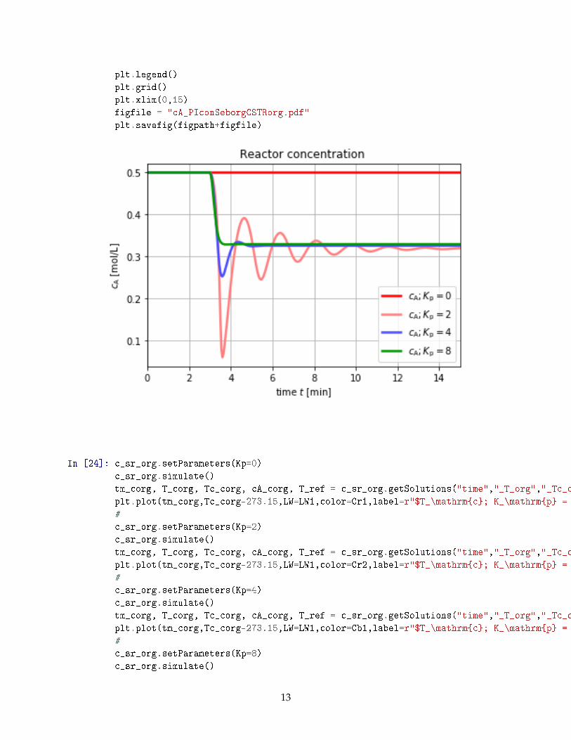
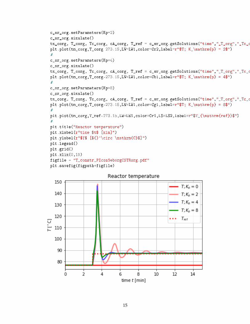
Observe. . . The design value for Kp based on a linear model does not give good performance;a larger control gain should be chosen to ensure decent performance for the nonlinear system. Wealso see that the controllers give negative cooling temperature, which is not realistic. Let us seewhat happens if we constrain the cooling temperature (the control input) to Tc > 4 [C].

In [25]: c_sr_org.setParameters(Tc_min = 4+273.15)


c_sr_org.simulate()



#

14


c_sr_org.simulate()



#


c_sr_org.simulate()


plt.plot(tm_corg,T_corg-273.15,LW=LW1,color=Cb1,label=r"$T; K_\mathrm{p} = 4$")

#


c_sr_org.simulate()


plt.plot(tm_corg,T_corg-273.15,LW=LW1,color=Cg1,label=r"$T; K_\mathrm{p} = 8$")

#

plt.plot(tm_corg,T_ref-273.15,LW=LW1,color=Cr1,LS=LS2,label=r"$T_{\mathrm{ref}}$")

#




plt.legend()

plt.grid()

plt.xlim(0,15)

figfile = "T_constr_PIconSeborgCSTRorg.pdf"


15


c_sr_org.simulate()



#


c_sr_org.simulate()



#


c_sr_org.simulate()


plt.plot(tm_corg,cA_corg,LW=LW1,color=Cb1,label=r"$c_\mathrm{A}; K_\mathrm{p} = 4$")

#


c_sr_org.simulate()


plt.plot(tm_corg,cA_corg,LW=LW1,color=Cg1,label=r"$c_\mathrm{A}; K_\mathrm{p} = 8$")

#

plt.title("Reactor concentration ")


plt.ylabel(r"$c_\mathrm{A}$ [mol/L]")

plt.legend()

plt.grid()

plt.xlim(0,15)

figfile = "cA_constr_PIconSeborgCSTRorg.pdf"


16


c_sr_org.simulate()



#


c_sr_org.simulate()



#


c_sr_org.simulate()


plt.plot(tm_corg,Tc_corg-273.15,LW=LW1,color=Cb1,label=r"$T_\mathrm{c}; K_\mathrm{p} = 4$")

#


c_sr_org.simulate()


plt.plot(tm_corg,Tc_corg-273.15,LW=LW1,color=Cg1,label=r"$T_\mathrm{c}; K_\mathrm{p} = 8$")

#

plt.title("Control signal: cooling temperature ")



17

plt.legend()

plt.grid()

plt.xlim(0,15)

figfile = "Tc_constr_PIconSeborgCSTRorg.pdf"


Observe. . . The constraint in the control input dramatically reduces the performance of thecontroller.

18

SeborgCSTR_complex_models

March 13, 2018


1.1 Complex models of “Seborg reactor”

1.1.1 Bernt Lie




import numpy as np


%matplotlib inline


import pandas as pd

LW1 = 2.5

LW2 = LW1/2

Cb1 = (0.3,0.3,1)

Cb2 = (0.7,0.7,1)

Cg1 = (0,0.6,0)

Cg2 = (0.5,0.8,0.5)

Cr1 = "Red"

Cr2 = (1,0.5,0.5)

LS1 = "solid"

LS2 = "dotted"

LS3 = "dashed"


1.1.3 Nonlinear reactor models based on Seborg et al.

Process diagram

Original state space model The original model is based on several simplifying assumptions: *Reaction species A, B are diluted in a solvent S. * The solvent dominates totally in the mixture, andwe can assume constant density in the reaction medium. * Due to constant density (and constantreactor volume), the influent and effluent volumetric flow rates are equal. * Because of dominanceof solvent, thermal parameters (heat capacities) are constant and independent of presence of A

1

and B. * The reaction order is set to unity, α = 1. * The heat of reaction is assumed independent oftemperature. * We need to include information about the amount of species B in the model.

Complex model 1: rho We maintain that the mixture density is constant, with constant volumet-ric flow rate through the reactor. However, * The thermal parameters (heat capacities) are allowedto vary with the concentrations of A and B. * We allow for general model order α. * With generalmodel order, the reaction enthalpy may vary with composition and temperature.

Complex model 1 will be given descriptive name related to rho, which indicates constant den-sity (ρ). The following is a DAE implementation in Modelica.

model ModSeborgCSTRrho

// Model of Seborg CSTR when assuming dominant solvent and Constant flow rate Vd



// November 7, 2017

//

// Parameters


parameter Real rho = 1e3 "Liquid density, g/L";

parameter Real m = rho*V "Reactor content mass, g";

parameter Real mS = m "Reactor solvent mass, g";





//

parameter Real HtA_o = 5e4 "Molar enthalpy of A at std state, J/mol";

parameter Real HtB_o = 0 "Molar enthalpy of B at std state, J/mol";

parameter Real HhS_o = 0 "Specific enthalpy of solvent at std state, J/g";

parameter Real cptA = 5 "Molar heat capacity of A, J/(mol.K)";

parameter Real cptB = cptA "Molar heat capacity of B, J/(mol.K)";

parameter Real cphS = 0.239 "Specific heat capacity of solvent, J/(g.K)";

parameter Real cph = cphS "Specific heat capacity of mixture, J/(g.K)";

parameter Real T_o = 293.15 "Temperature in std state, K";

parameter Real p_o = 1.01e5 "Pressure in std state, Pa";



parameter Real nA0 = cA0*V "Initial number of moles of A, mol";

parameter Real nB0 = 0 "Initial number of moles of B, mol";


parameter Real HtA0 = HtA_o + cptA*(T0-T_o) "Initial pure molar enthalpy of A, J/mol";

parameter Real HtB0 = HtB_o + cptB*(T0-T_o) "Initial pure molar enthalpy of B, J/mol";

parameter Real HhS0 = HhS_o + cphS*(T0-T_o) "Initial pure specific enthalpy of solvent, J/g";

parameter Real HA0 = nA0*HtA0 "Initial pure enthalpy of A, J";

parameter Real HB0 = nB0*HtB0 "Initial pure enthalpy of B, J";

parameter Real HS0 = mS*HhS0 "Initial pure enthalpy of solvent, J";

parameter Real H0 = HA0 + HB0 + HS0 "Initial total enthalpy of ideal solution, J";

parameter Real U0 = H0 - p_o*V "Initial internal energy, J";

2


// -- states

Real nA(start = nA0, fixed = true) "Initializing amount of A in reactor, mol";

Real nB(start = nB0, fixed = true) "Initializing amount of B in reactor, mol";

Real U(start = U0, fixed = true) "Initializing internal energy in reactor, J";


Real ndAi "Influent molar flow rate of A, mol/s";

Real ndAe "Effluent molar flow rate of A, mol/s";

Real ndAg "Molar rate of generation of A, mol/s";

Real ndBi "Influent molar flow rate of B, mol/s";

Real ndBe "Effluent molar flow rate of B, mol/s";

Real ndBg "Molar rate of generation of B, mol/s";

Real mdSi "Influent mass flow rate of solvent, g/min";

Real mdSe "Effluent mass flow rate of solvent, g/min";

Real Hdi "Influent enthalpy flow rate, J/min";

Real Hde "Effluent enthalpy flow rate, J/min";

Real cA "Molar concentration of A, mol/L";

Real cB "Molar concentration of B, mol/L";


Real T "Reactor temperature, K";


Real H "Reactor enthalpy, J";

Real HA "Enthalpy of pure A, J";

Real HB "Enthalpy of pure B, J";

Real HS "Enthalpy of pure solvent, J";

Real HtA "Molar enthalpy of pure A, J/mol";

Real HtB "Molar enthalpy of pure B, J/mol";

Real HhS "Specific enthalpy of pure solvent, J/g";

Real HdAi "Influent enthalpy flow of pure A,J/min";

Real HdBi "Influent enthalpy flow of pure B, J/min";

Real HdSi "Influent enthalpy flow of pure solvent, J/min";

Real HtAi "Influent molar enthalpy of pure A, J/mol";

Real HtBi "Influent molar enthalpy of pure B, J/mol";

Real HhSi "Influent specific enthalpy of solvent, J/g";

Real HdAe "Effluent enthalpy flow of pure A, J/min";

Real HdBe "Effluent enthalpy flow of pure B, J/min";

Real HdSe "Effluent enthalpy flow of pure solvent, J/min";



input Real Vdi "Volumetric flow rate through reactor, L/s";



input Real Tc "Cooling temperature, K";



output Real y_cB "Molar concentration of B, mol/L";


equation

3


der(nA) = ndAi - ndAe + ndAg;

der(nB) = ndBi - ndBe + ndBg;

der(U) = Hdi - Hde + Qd;


nA = cA*V;

nB = cB*V;

ndAi = cAi*Vdi;

ndBi = 0;

mdSi = rho*Vdi;

ndAe = cA*Vdi;

ndBe = cB*Vdi;

mdSe = mdSi;

ndAg = -a*r*V;

ndBg = r*V;

r = k*cAâ;

k = k0*exp(-EdR/T);

U = H-p_o*V;

H = HA + HB + HS;

HA = nA*HtA;

HB = nB*HtB;

HS = mS*HhS;

HtA = HtA_o + cptA*(T-T_o);

HtB = HtB_o + cptB*(T-T_o);

HhS = HhS_o + cphS*(T-T_o);

Hdi = HdAi + HdBi + HdSi;

HdAi = ndAi*HtAi;

HdBi = ndBi*HtBi;

HdSi = mdSi*HhSi;

HtAi = HtA_o + cptA*(Ti-T_o);

HtBi = 0;

HhSi = HhS_o + cphS*(Ti-T_o);

Hde = HdAe + HdBe + HdSe;

HdAe = ndAe*HtA;

HdBe = ndBe*HtB;

HdSe = mdSe*HhS;

Qd = UA*(Tc-T);

// Outputs

y_T = T;

y_cB = cB;

end ModSeborgCSTRrho;

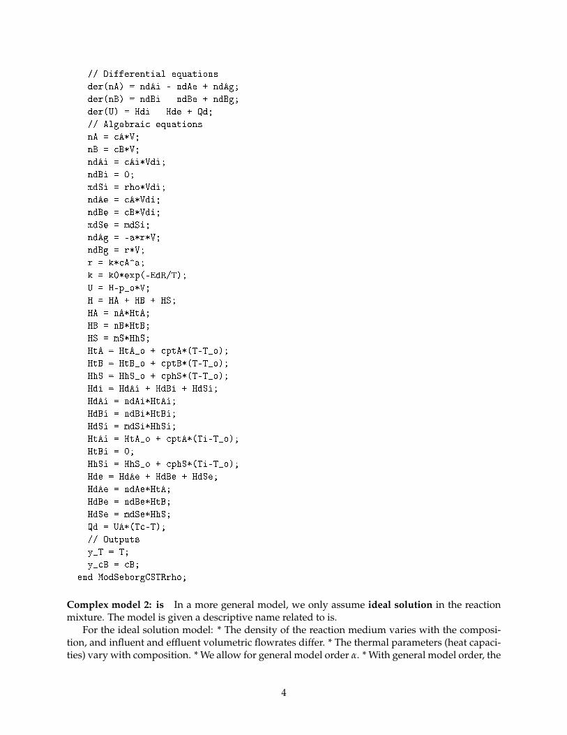
Complex model 2: is In a more general model, we only assume ideal solution in the reactionmixture. The model is given a descriptive name related to is.

For the ideal solution model: * The density of the reaction medium varies with the composi-tion, and influent and effluent volumetric flowrates differ. * The thermal parameters (heat capaci-ties) vary with composition. * We allow for general model order α. * With general model order, the

4

reaction enthalpy will vary with composition and temperature. * We need to include informationabout the amount of species B in the model.

It is relatively straightforward to develop a DAE model for this case. It is also possible todevelop an ODE model: this time, we need three states (we need to include information aboutspecies B). The ODE formulation is simpler than the DAE model, but it is relatively complicatedto develop the ODE model. The DAE model is as follows:

model ModSeborgCSTRis

// Model of Seborg CSTR when assuming Ideal Solution, only



// November 7, 2017

//

// Parameters

parameter Real rhoS_o = 1e3 "Density of pure S, g/L";

parameter Real rhoA_o = 1.5e3 "Density of pure A, g/L";

parameter Real rhoB_o = 2.5e3 "Density of pure B, g/L";

parameter Real MA = 50 "Molar mass of A, g/mol";

parameter Real MB = MA*a "Molar mass of B, g/mol";





parameter Real p_o = 1.01e5 "Pressure in std state, Pa";

//

parameter Real HhS_o = 0 "Specific enthalpy of solvent at std state, J/g";

parameter Real HtA_o = 5e4 "Molar enthalpy of A at std state, J/mol";

parameter Real HtB_o = 0 "Molar enthalpy of B at std state, J/mol";

//

parameter Real cphS = 0.239 "Specific heat capacity of solvent, J/(g.K)";

parameter Real cptA = 5 "Molar heat capacity of A, J/(mol.K)";

parameter Real cptB = cptA "Molar heat capacity of B, J/(mol.K)";

//

parameter Real T_o = 293.15 "Temperature in std state, K";

//




parameter Real nA0 = cA0*V "Initial number of moles of A, mol";

parameter Real nB0 = 0 "Initial number of moles of B, mol";

parameter Real mA0 = nA0*MA "Initial mass of A, g";

parameter Real mB0 = nB0*MB "Initial mass of B, g";

parameter Real VA0 = mA0/rhoA_o "Initial volume of A, L";

parameter Real VB0 = mB0/rhoB_o "Initial volume of B, L";

parameter Real VS0 = V - VA0 - VB0 "Initial volume of S, L";

parameter Real mS0 = VS0*rhoS_o "Initial mass of S, g";


parameter Real HhS0 = HhS_o + cphS*(T0-T_o) "Initial pure specific enthalpy of solvent, J/g";

5

parameter Real HtA0 = HtA_o + cptA*(T0-T_o) "Initial pure molar enthalpy of A, J/mol";

parameter Real HtB0 = HtB_o + cptB*(T0-T_o) "Initial pure molar enthalpy of B, J/mol";

parameter Real HS0 = mS0*HhS0 "Initial pure enthalpy of solvent, J";

parameter Real HA0 = nA0*HtA0 "Initial pure enthalpy of A, J";

parameter Real HB0 = nB0*HtB0 "Initial pure enthalpy of B, J";

parameter Real H0 = HS0 + HA0 + HB0 "Initial total enthalpy of ideal solution, J";

parameter Real U0 = H0 - p_o*V "Initial internal energy, J";


// -- states

Real mS(start = mS0) "Initial amount of S in reactor, kg";

Real nA(start = nA0, fixed = true) "Initializing amount of A in reactor, mol";

Real nB(start = nB0, fixed = true) "Initializing amount of B in reactor, mol";

Real U(start = U0, fixed = true) "Initializing internal energy in reactor, J";


// Real mS "Mass of S, g";

Real V_x;

Real mdSi "Influent mass flow rate of S, g/s";

Real mdSe "Effluent mass flow rate of S, g/s";

Real ndAi "Influent molar flow rate of A, mol/s";

Real ndAe "Effluent molar flow rate of A, mol/s";

Real ndAg "Molar rate of generation of A, mol/s";

Real ndBi "Influent molar flow rate of B, mol/s";

Real ndBe "Effluent molar flow rate of B, mol/s";

Real ndBg "Molar rate of generation of B, mol/s";

Real Hdi "Influent enthalpy flow rate, J/min";

Real Hde "Effluent enthalpy flow rate, J/min";


//

Real VS "Volume of pure S, L";

Real VA "Volume of pure A, L";

Real VB "Volume of pure B, L";

Real mA "Mass of A, g";

Real mB "Mass of B, g";

//

Real Vde "Effluent volumetric flow rate, L/min";

//

Real rhoS "Specific concentration of S, g/L";

Real cA "Molar concentration of A, mol/L";

Real cB "Molar concentration of B, mol/L";



Real T "Absolute temperature, K";

//

Real H "Reactor enthalpy, J";

Real HS "Enthalpy of pure solvent, J";

Real HA "Enthalpy of pure A, J";

Real HB "Enthalpy of pure B, J";

Real HhS "Specific enthalpy of pure solvent, J/g";

6

Real HtA "Molar enthalpy of pure A, J/mol";

Real HtB "Molar enthalpy of pure B, J/mol";

Real HdSi "Influent enthalpy flow of pure solvent, J/min";

Real HdAi "Influent enthalpy flow of pure A,J/min";

Real HdBi "Influent enthalpy flow of pure B, J/min";

Real HhSi "Influent specific enthalpy of solvent, J/g";

Real HtAi "Influent molar enthalpy of pure A, J/mol";

Real HtBi "Influent molar enthalpy of pure B, J/mol";

Real HdSe "Effluent enthalpy flow of pure solvent, J/min";

Real HdAe "Effluent enthalpy flow of pure A, J/min";

Real HdBe "Effluent enthalpy flow of pure B, J/min";

//

Real mdSi_x;


input Real Vdi "Volumetric flow rate through reactor, L/s";



input Real Tc "Cooling temperature, K";



output Real y_cB "Molar concentration of B, mol/L";


equation


mdSi_x = mdSe + der(mS);

der(mS) = mdSi - mdSe;

der(nA) = ndAi - ndAe + ndAg;

der(nB) = ndBi - ndBe + ndBg;

der(U) = Hdi - Hde + Qd;


V = VS + VA + VB;

VS = mS/rhoS_o;

VA = mA/rhoA_o;

VB = mB/rhoB_o;

mS = rhoS*V;

V_x = mS/rhoS_o + nA*MA/rhoA_o + nB*MB/rhoB_o;

mA = nA*MA;

mB = nB*MB;

nA = cA*V;

nB = cB*V;

//

mdSi = rhoS_o*(1-cAi*MA/rhoA_o)*Vdi;

ndAi = cAi*Vdi;

ndBi = 0;

mdSe = rhoS*Vde;

ndAe = cA*Vde;

ndBe = cB*Vde;

7

ndAg = -a*r*V;

ndBg = r*V;

r = k*cAâ;

k = k0*exp(-EdR/T);

//

U = H-p_o*V;

H = HS + HA + HB;

HS = mS*HhS;

HA = nA*HtA;

HB = nB*HtB;

//

HhS = HhS_o + cphS*(T-T_o);

HtA = HtA_o + cptA*(T-T_o);

HtB = HtB_o + cptB*(T-T_o);

//

Hdi = HdSi + HdAi + HdBi;

HdSi = mdSi*HhSi;

HdAi = ndAi*HtAi;

HdBi = ndBi*HtBi;

//

HhSi = HhS_o + cphS*(Ti-T_o);

HtAi = HtA_o + cptA*(Ti-T_o);

HtBi = 0;

//

Hde = HdAe + HdBe + HdSe;

HdSe = mdSe*HhS;

HdAe = ndAe*HtA;

HdBe = ndBe*HtB;

//

Qd = UA*(Tc-T);

// Outputs

y_T = T;

y_cB = cB;

end ModSeborgCSTRis;

1.1.4 Comparing models

Instantiating models

In [2]: sr_is = ModelicaSystem("SeborgCSTR.mo","SeborgCSTR.ModSeborgCSTRis")

sr_rho = ModelicaSystem("SeborgCSTR.mo","SeborgCSTR.ModSeborgCSTRrho")

sr_org = ModelicaSystem("SeborgCSTR.mo","SeborgCSTR.ModSeborgCSTRorg")

2018-03-13 14:58:39,841 - OMPython - INFO - OMC Server is up and running at file:///c:/users/bernt_~1/appdata/local/temp/openmodelica.port.64db13e12d244d7a81c9dd908e64251d

2018-03-13 14:58:43,240 - OMPython - INFO - OMC Server is up and running at file:///c:/users/bernt_~1/appdata/local/temp/openmodelica.port.2b67f6301a2747e29cf7bef13161385c

2018-03-13 14:58:46,236 - OMPython - INFO - OMC Server is up and running at file:///c:/users/bernt_~1/appdata/local/temp/openmodelica.port.18969db823ec44319522b5f7ad280ca6

8

Setting up simulations

In [3]: sr_is.setSimulationOptions(stopTime=15,stepSize=0.05)

sr_rho.setSimulationOptions(stopTime=15,stepSize=0.05)

sr_org.setSimulationOptions(stopTime=15,stepSize=0.05)

#

sr_is.setInputs(Tc=300)

sr_is.setInputs(Ti=350)

sr_is.setInputs(Vdi=100)

sr_is.setInputs(cAi=1)

sr_rho.setInputs(Tc=300)

sr_rho.setInputs(Ti=350)

sr_rho.setInputs(Vdi=100)

sr_rho.setInputs(cAi=1)

sr_org.setInputs(Tc=300)




Simulating system for three cases of inputs, and extracting results

In [4]: sr_is.setInputs(Tc=300)

sr_is.simulate()

tm_is0, T_is0, Tc_is0, cA_is0 = sr_is.getSolutions("time","T","Tc","cA")

sr_is.setInputs(Tc=300+5)

sr_is.simulate()

tm_is0p, T_is0p, Tc_is0p, cA_is0p = sr_is.getSolutions("time","T","Tc","cA")

sr_is.setInputs(Tc=300-10)

sr_is.simulate()

tm_is0m, T_is0m, Tc_is0m, cA_is0m = sr_is.getSolutions("time","T","Tc","cA")

In [5]: sr_rho.setInputs(Tc=300)

sr_rho.simulate()

tm_rho0, T_rho0, Tc_rho0, cA_rho0 = sr_rho.getSolutions("time","T","Tc","cA")

sr_rho.setInputs(Tc=300+5)

sr_rho.simulate()

tm_rho0p, T_rho0p, Tc_rho0p, cA_rho0p = sr_rho.getSolutions("time","T","Tc","cA")

sr_rho.setInputs(Tc=300-10)

sr_rho.simulate()

tm_rho0m, T_rho0m, Tc_rho0m, cA_rho0m = sr_rho.getSolutions("time","T","Tc","cA")


sr_org.simulate()

tm_org0, T_org0, Tc_org0, cA_org0 = sr_org.getSolutions("time","T","Tc","cA")

sr_org.setInputs(Tc=300+5)

sr_org.simulate()

tm_org0p, T_org0p, Tc_org0p, cA_org0p = sr_org.getSolutions("time","T","Tc","cA")

sr_org.setInputs(Tc=300-10)

sr_org.simulate()

tm_org0m, T_org0m, Tc_org0m, cA_org0m = sr_org.getSolutions("time","T","Tc","cA")

9

Plotting results

In [7]: plt.plot(tm_org0,T_org0-273.15,LW=LW1,color=Cg1,label=r"$T_{\mathrm{c,org}}^{\ast}$")

plt.plot(tm_org0p,T_org0p-273.15,LW=LW1,color=Cr1,label=r"$T_{\mathrm{c,org}}^{\ast}+5$")

plt.plot(tm_org0m,T_org0m-273.15,LW=LW1,color=Cb1,label=r"$T_{\mathrm{c,org}}^{\ast}-10$")

plt.plot(tm_rho0,T_rho0-273.15,LW=LW1,LS=LS2,color=Cg2,label=r"$T_{\mathrm{c,\rho}}^{\ast}$")

plt.plot(tm_rho0p,T_rho0p-273.15,LW=LW1,LS=LS2,color=Cr2,label=r"$T_{\mathrm{c,\rho}}^{\ast}+5$")

plt.plot(tm_rho0m,T_rho0m-273.15,LW=LW1,LS=LS2,color=Cb2,label=r"$T_{\mathrm{c,\rho}}^{\ast}-10$")

plt.plot(tm_is0,T_is0-273.15,LW=LW1,LS=LS3,color=Cg2,label=r"$T_{\mathrm{c,is}}^{\ast}$")

plt.plot(tm_is0p,T_is0p-273.15,LW=LW1,LS=LS3,color=Cr2,label=r"$T_{\mathrm{c,is}}^{\ast}+5$")

plt.plot(tm_is0m,T_is0m-273.15,LW=LW1,LS=LS3,color=Cb2,label=r"$T_{\mathrm{c,is}}^{\ast}-10$")

plt.legend(ncol=3)




plt.grid()

plt.xlim(0,15)

figfile = "tempSeborgCSTR.pdf"


In [8]: plt.plot(tm_org0,cA_org0,LW=LW1,color=Cg1,label=r"$T_{\mathrm{c,org}}^{\ast}$")

plt.plot(tm_org0p,cA_org0p,LW=LW1,color=Cr1,label=r"$T_{\mathrm{c,org}}^{\ast}+5$")

plt.plot(tm_org0m,cA_org0m,LW=LW1,color=Cb1,label=r"$T_{\mathrm{c,org}}^{\ast}-10$")

plt.plot(tm_rho0,cA_rho0,LW=LW1,LS=LS2,color=Cg2,label=r"$T_{\mathrm{c,\rho}}^{\ast}$")

10

plt.plot(tm_rho0p,cA_rho0p,LW=LW1,LS=LS2,color=Cr2,label=r"$T_{\mathrm{c,\rho}}^{\ast}+5$")

plt.plot(tm_rho0m,cA_rho0m,LW=LW1,LS=LS2,color=Cb2,label=r"$T_{\mathrm{c,\rho}}^{\ast}-10$")

plt.plot(tm_is0,cA_is0,LW=LW1,LS=LS3,color=Cg2,label=r"$T_{\mathrm{c,is}}^{\ast}$")

plt.plot(tm_is0p,cA_is0p,LW=LW1,LS=LS3,color=Cr2,label=r"$T_{\mathrm{c,is}}^{\ast}+5$")

plt.plot(tm_is0m,cA_is0m,LW=LW1,LS=LS3,color=Cb2,label=r"$T_{\mathrm{c,is}}^{\ast}-10$")


plt.title("Concentration of $\mathrm{A}$")


plt.ylabel(r"$c_{\mathrm{A}}$ [mol/L]")

plt.grid()

plt.xlim(0,15)

figfile = "concSeborgCSTR.pdf"


In [9]: plt.plot(tm_org0,Tc_org0-273.15,LW=LW1, color=Cg1, label=r"$T_\mathrm{c}^{\ast}$")

plt.plot(tm_org0p,Tc_org0p-273.15,LW=LW1,color=Cr1, label=r"$T_\mathrm{c}^{\ast}+5$")

plt.plot(tm_org0m,Tc_org0m-273.15,LW=LW1,color=Cb1, label=r"$T_\mathrm{c}^{\ast}-10$")

plt.title("Cooling liquid temperature")

plt.xlabel(r"time $t$ [s]")


plt.grid()

plt.axis(ymin=15,ymax=35)

plt.xlim(0,15)

11


figfile = "coolSeborgCSTR.pdf"


12

SeborgCSTR_sensitivity

March 13, 2018


1.1 Sensitivity analysis of “Seborg reactor”

1.1.1 Bernt Lie




import numpy as np


%matplotlib inline


import pandas as pd

LW1 = 2.5

LW2 = LW1/2

Cb1 = (0.3,0.3,1)

Cb2 = (0.7,0.7,1)

Cg1 = (0,0.6,0)

Cg2 = (0.5,0.8,0.5)

Cr1 = "Red"

Cr2 = (1,0.5,0.5)

LS1 = "solid"

LS2 = "dotted"

LS3 = "dashed"


1.1.3 Reactor temperature sensitivity to UA from Monte Carlo simulations

Instantiating models and setting inputs

In [2]: srp = ModelicaSystem("SeborgCSTR.mo","SeborgCSTR.ModSeborgCSTRorg")

srm = ModelicaSystem("SeborgCSTR.mo","SeborgCSTR.ModSeborgCSTRorg")

2018-03-13 14:56:13,187 - OMPython - INFO - OMC Server is up and running at file:///c:/users/bernt_~1/appdata/local/temp/openmodelica.port.87eccc84be1c43f98348f84d164621a8

2018-03-13 14:56:16,158 - OMPython - INFO - OMC Server is up and running at file:///c:/users/bernt_~1/appdata/local/temp/openmodelica.port.e8697dcbd5f045fe9acb19fa0d0f0480

1

In [3]: srp.setSimulationOptions(stopTime=10,stepSize=0.05)

srm.setSimulationOptions(stopTime=10,stepSize=0.05)

#

srp.setInputs(Tc=300+5)

srm.setInputs(Tc=300-10)

srp.setInputs(Ti=350,Vdi=100,cAi=1)

srm.setInputs(Ti=350,Vdi=100,cAi=1)

Finding parameter names, and generating random variations of UA with uniform distributionand 5% variation

In [4]: p = srp.getParameters()

p.keys()

Out[4]: ['a', 'cph', 'DrHt', 'cA0', 'T0', 'EdR', 'k0', 'rho', 'V', 'UA']

In [5]: p.values()

Out[5]: [1.0, 0.239, -50000.0, 0.5, 350.0, 8750.0, None, 1000.0, 100.0, 50000.0]

In [6]: UA = p["UA"]

UA

Out[6]: 50000.0

In [7]: nr.seed(0)

UUAA = UA*(1 + (nr.rand(20)-0.5)/2)

Simulating for nominal values UA of UA, as well as for random variations in UA

In [8]: srp.simulate()

tm0p,T0p = srp.getSolutions("time","T")

srm.simulate()

tm0m,T0m = srm.getSolutions("time","T")

#

for ua in UUAA:

srp.setParameters(UA=ua);

srp.simulate()

tm0p1,T0p1 = srp.getSolutions("time","T")

srm.setParameters(UA=ua);

srm.simulate()

tm0m1,T0m1 = srm.getSolutions("time","T")

plt.plot(tm0p1,T0p1-273.15,LW=LW2,color=Cr1,LS=LS2,label="_nolabel_")

plt.plot(tm0m1,T0m1-273.15,LW=LW2,color=Cb1,LS=LS2,label="_nolabel_")

#

plt.plot(tm0p,T0p-273.15,LW=LW1,color=Cr1,label=r"$\overline{UA} : T_c^{\ast}+5$")

plt.plot(tm0m,T0m-273.15,LW=LW1,color=Cb1,label=r"$\overline{UA} : T_c^{\ast}-10$")

plt.title("Reactor temperature Monte Carlo study")

plt.xlabel(r"time $t$ [s]")

2


plt.grid()

plt.xlim(0,10)

plt.legend()

figfile = "sensitivitySeborgCSTRorg.pdf"


1.1.4 Sensitivity of quantities wrt. parameters


2018-03-13 14:56:28,186 - OMPython - INFO - OMC Server is up and running at file:///c:/users/bernt_~1/appdata/local/temp/openmodelica.port.7b7305021dca41b9a2e4f92b2ab828d7

In [10]: sr_org.setSimulationOptions(stopTime=20)





In [12]: sr_org.simulate()

tm = sr_org.getSolutions("time")

3

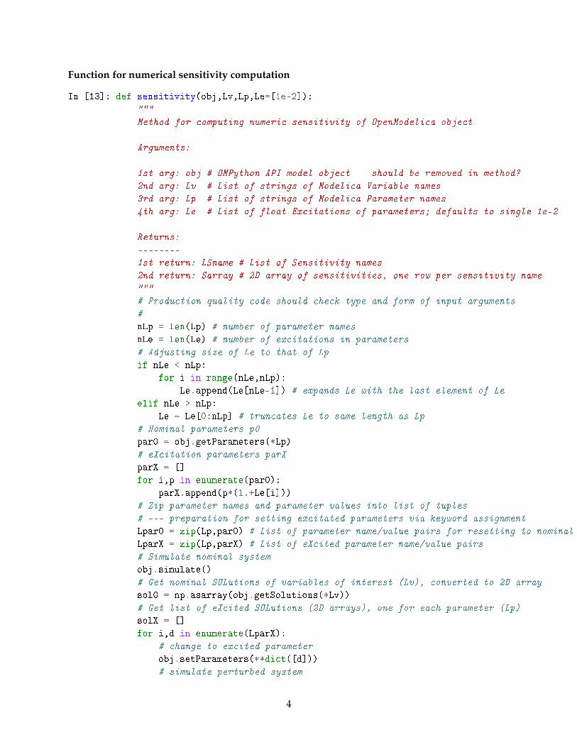
Function for numerical sensitivity computation

In [13]: def sensitivity(obj,Lv,Lp,Le=[1e-2]):

"""

Method for computing numeric sensitivity of OpenModelica object

Arguments:

----------

1st arg: obj # OMPython API model object -- should be removed in method?

2nd arg: Lv # List of strings of Modelica Variable names

3rd arg: Lp # List of strings of Modelica Parameter names

4th arg: Le # List of float Excitations of parameters; defaults to single 1e-2

Returns:

--------

1st return: LSname # List of Sensitivity names

2nd return: Sarray # 2D array of sensitivities, one row per sensitivity name

"""

# Production quality code should check type and form of input arguments

#

nLp = len(Lp) # number of parameter names

nLe = len(Le) # number of excitations in parameters

# Adjusting size of Le to that of Lp

if nLe < nLp:

for i in range(nLe,nLp):

Le.append(Le[nLe-1]) # expands Le with the last element of Le

elif nLe > nLp:

Le = Le[0:nLp] # truncates Le to same length as Lp

# Nominal parameters p0

par0 = obj.getParameters(*Lp)

# eXcitation parameters parX

parX = []

for i,p in enumerate(par0):

parX.append(p*(1.+Le[i]))

# Zip parameter names and parameter values into list of tuples

# --- preparation for setting excitated parameters via keyword assignment

Lpar0 = zip(Lp,par0) # List of parameter name/value pairs for resetting to nominal case

LparX = zip(Lp,parX) # List of eXcited parameter name/value pairs

# Simulate nominal system

obj.simulate()

# Get nominal SOLutions of variables of interest (Lv), converted to 2D array

sol0 = np.asarray(obj.getSolutions(*Lv))

# Get list of eXcited SOLutions (2D arrays), one for each parameter (Lp)

solX = []

for i,d in enumerate(LparX):

# change to excited parameter

obj.setParameters(**dict([d]))

# simulate perturbed system

4

obj.simulate()

# get eXcited SOLutions (Lv) as 2D array, and append to list

solX.append(np.asarray(obj.getSolutions(*Lv)))

# reset parameters to nominal values

obj.setParameters(**dict(Lpar0))

# Compute sensitivities and add to list, one 2D array per parameter (Lp)

LSname = [] # Preparing list of names of sensitivities

LSarray = [] # Preparing list of 2d sensitivity arrays, 1 per parameter

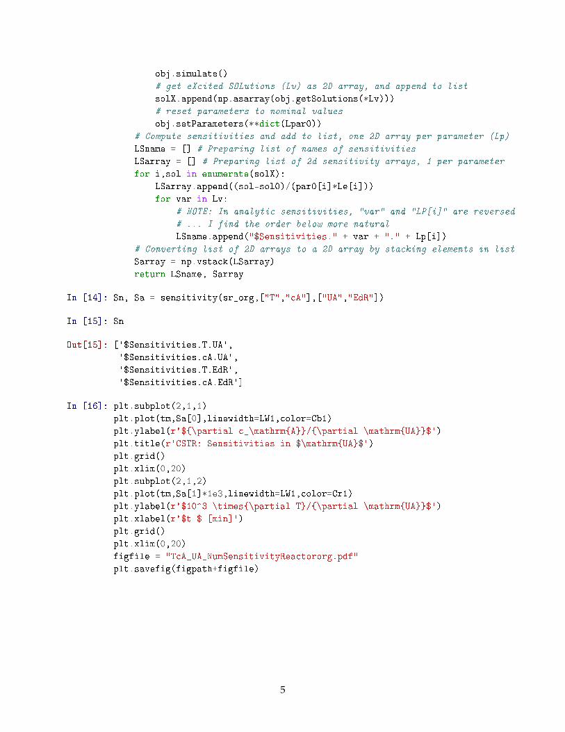
for i,sol in enumerate(solX):

LSarray.append((sol-sol0)/(par0[i]*Le[i]))

for var in Lv:

# NOTE: In analytic sensitivities, "var" and "LP[i]" are reversed

# ... I find the order below more natural

LSname.append("$Sensitivities." + var + "." + Lp[i])

# Converting list of 2D arrays to a 2D array by stacking elements in list

Sarray = np.vstack(LSarray)

return LSname, Sarray

In [14]: Sn, Sa = sensitivity(sr_org,["T","cA"],["UA","EdR"])

In [15]: Sn

Out[15]: ['$Sensitivities.T.UA',

'$Sensitivities.cA.UA',

'$Sensitivities.T.EdR',

'$Sensitivities.cA.EdR']

In [16]: plt.subplot(2,1,1)

plt.plot(tm,Sa[0],linewidth=LW1,color=Cb1)

plt.ylabel(r'${\partial c_\mathrm{A}}/{\partial \mathrm{UA}}$')

plt.title(r'CSTR: Sensitivities in $\mathrm{UA}$')

plt.grid()

plt.xlim(0,20)

plt.subplot(2,1,2)

plt.plot(tm,Sa[1]*1e3,linewidth=LW1,color=Cr1)

plt.ylabel(r'$10^3 \times{\partial T}/{\partial \mathrm{UA}}$')

plt.xlabel(r'$t $ [min]')

plt.grid()

plt.xlim(0,20)

figfile = "TcA_UA_NumSensitivityReactororg.pdf"


5

In [17]: plt.subplot(2,1,1)

plt.plot(tm,Sa[2],linewidth=LW1,color=Cb1)

plt.ylabel(r'${\partial c_\mathrm{A}}/{\partial (E/R)}$')

plt.title(r'CSTR: Sensitivities in $E/R$')

plt.grid()

plt.xlim(0,20)

plt.subplot(2,1,2)

plt.plot(tm,Sa[3]*1e3,linewidth=LW1,color=Cr1)

plt.ylabel(r'$10^3 \times{\partial T}/{\partial (E/R)}$')

plt.xlabel(r'$t $ [min]')

plt.grid()

plt.xlim(0,20)

figfile = "TcA_EdR_NumSensitivitySeborgCSTRorg.pdf"


6

Here, numerical sensitivity has been computed. OpenModelica has support for computinganalytic sensitivities, but that has not been properly interfaced to the Python API at the moment.

7

Date post:	01-Sep-2018
Category:	Documents
Upload:	phungque
View:	235 times
Download:	0 times

SeborgCSTR basics - openmodelica.org · Modelica code for original Seborg et al model...

Documents