Second-harmonic generation and the conservationof spatiotemporal orbital angular momentum oflightGuan Gui 

JILA, University of Colorado BoulderNathan Brooks 

JILA, University of Colorado BoulderHenry Kapteyn 

Joint Institute for Laboratory AstrophysicsMargaret Murnane 

JILA, University of Colorado BoulderChen-Ting Liao  ( chenting.liao@gmail.com )

University of Colorado Boulder https://orcid.org/0000-0002-3423-277X

Article

Keywords: Space-time Spiral Phase Structure, Nonlinear Scaling Rule, Spatiotemporal Astigmatism,Multiple Phase Singularities, Nonlinear Conversion

Posted Date: December 10th, 2020

DOI: https://doi.org/10.21203/rs.3.rs-116263/v1

License: This work is licensed under a Creative Commons Attribution 4.0 International License.  Read Full License

Version of Record: A version of this preprint was published at Nature Photonics on July 5th, 2021. See thepublished version at https://doi.org/10.1038/s41566-021-00841-8.

1  

SECOND-HARMONIC GENERATION AND THE CONSERVATION OF

SPATIOTEMPORAL ORBITAL ANGULAR MOMENTUM OF LIGHT

GUAN GUI,1 NATHAN J. BROOKS,1 HENRY KAPTEYN,1,2 MARGARET MURNANE,1 AND CHEN-TING LIAO1*

1JILA, University of Colorado and NIST, 440 UCB, Boulder, Colorado 80309, USA

2KMLabs Inc., 4775 Walnut Street, Suite 102, Boulder, Colorado 80301, USA

*chenting.liao@colorado.edu

Abstract

Light with spatiotemporal orbital angular momentum (ST-OAM) is a recently discovered type of

structured electromagnetic field with characteristic space-time spiral phase structure and

transverse OAM. In this work, we present the first generation and characterization of the second-

harmonic of ST-OAM pulses. By uncovering the conservation of transverse OAM in a second-

harmonic generation process, where the space-time topological charge of the fundamental field is

doubled along with the optical frequency, we establish a general nonlinear scaling rule—

analogous to that describing the spatial topological charges associated with the conventional

longitudinal OAM of light. Furthermore, we observe that the topology of a second-harmonic ST-

OAM pulse can be modified by complex spatiotemporal astigmatism, giving rise to multiple phase

singularities separated in space and time. Our finding thus confirms that a spatiotemporal phase

winding, surrounding one or many phase singularities in space and time, can be interpreted as a

new class of topological charge. Our study opens a new route for nonlinear conversion and scaling

of light carrying ST-OAM with the potential for driving other secondary ST-OAM sources of

electromagnetic fields, electron pulses, and beyond.

2  

Introduction

The orbital angular momentum (OAM) of light is a type of angular momentum associated with

phase front vortices in the electromagnetic field1,2. For a propagating paraxial wave, the

longitudinal OAM of light means that the OAM is parallel to the averaged wavevector and

propagation direction of the beam. In addition, OAM can be intrinsic or extrinsic –-intrinsic OAM

implies that the angular momentum is independent of the choice of the reference frame and can be

described by an integer quantum number called the (spatial) topological charge ℓ . The intrinsic

longitudinal OAM (here referred to as conventional OAM) of light has an OAM of ℏℓ per photon

and a spiral phase structure 𝑒 ℓ , , surrounding a phase singularity in the x-y plane (see Fig.

1a). Most research efforts over the past three decades have focused on conventional OAM of light,

which has impacted many important applications –– including optical tweezers, super resolution

imaging, quantum and classical communication, and others3–5 ,9. Very recently, pulses with time-

varying OAM, or self-torque, have been discovered18.

In contrast, a transverse OAM of light implies that the OAM is perpendicular to the

averaged wavevector of the beam. This means that a spiral phase structure resides in space-time,

e.g., the x-t (or equivalently, the x-z) plane in a simplified 2D case (see Fig. 1a), and is thus referred

to as spatiotemporal orbital angular momentum (ST-OAM). By analogy with conventional OAM,

we can designate an integer ℓ as the spatiotemporal topological charge to describe the space-time

winding phase 𝑒 ℓ , , . The scalar field of an ST-OAM pulse reads - 𝐸 𝑥, 𝑦, 𝑧, 𝑡 ∝ 𝐸 𝑥,𝑦, 𝑧 𝑒 ℓ , , 𝑒 ,

where 𝐸 is the field envelope including the assumed Gaussian profile in the y-axis for simplicity.

This transverse OAM of light was theoretically predicted8,9, and generated through a nonlinear

self-focusing process10. Very recently, optical pulses with ST-OAM were experimentally realized

3  

in the linear regime for the first time11,12. We note that the ST-OAM of light was only recently

discovered, and many of its properties are still not known. Therefore, the extent to which they can

be described by an analogy with the conventional OAM of light remains unclear.

In nonlinear frequency conversion, the conventional OAM of light follows a simple scaling

rule, where the N-th harmonic has a topological charge Nℓ , reflecting OAM conservation. This

rule has been verified for SHG 13,14, non-perturbative high-order (N >10) harmonic generation15,

and can be generalized to describe sum- or difference-frequency generation processes16. Note that

this rule only applies to scalar fields without spin angular momentum, otherwise total angular

momentum conservation must be included17.

In this manuscript, we experimentally investigate the behavior of ST-OAM pulses during

the frequency up-conversion process of second-harmonic generation (SHG). By experimentally

uncovering the conservation of ST-OAM in a second-harmonic generation process, where the

space-time topological charge of the fundamental field is doubled along with the optical frequency,

we establish a general nonlinear scaling rule for the first time—analogous to that describing the

spatial topological charges in conventional OAM of light. We also investigate the effects of

spatiotemporal astigmatism in SHG, which leads to non-conserved topological changes of the

spiral phase structure, and the creation of multiple phase singularities separated in space-time. Our

finding thus confirms that this spatiotemporal phase winding, surrounding one or many phase

singularities in space and time, can be interpreted as a new class of topological charge.

4  

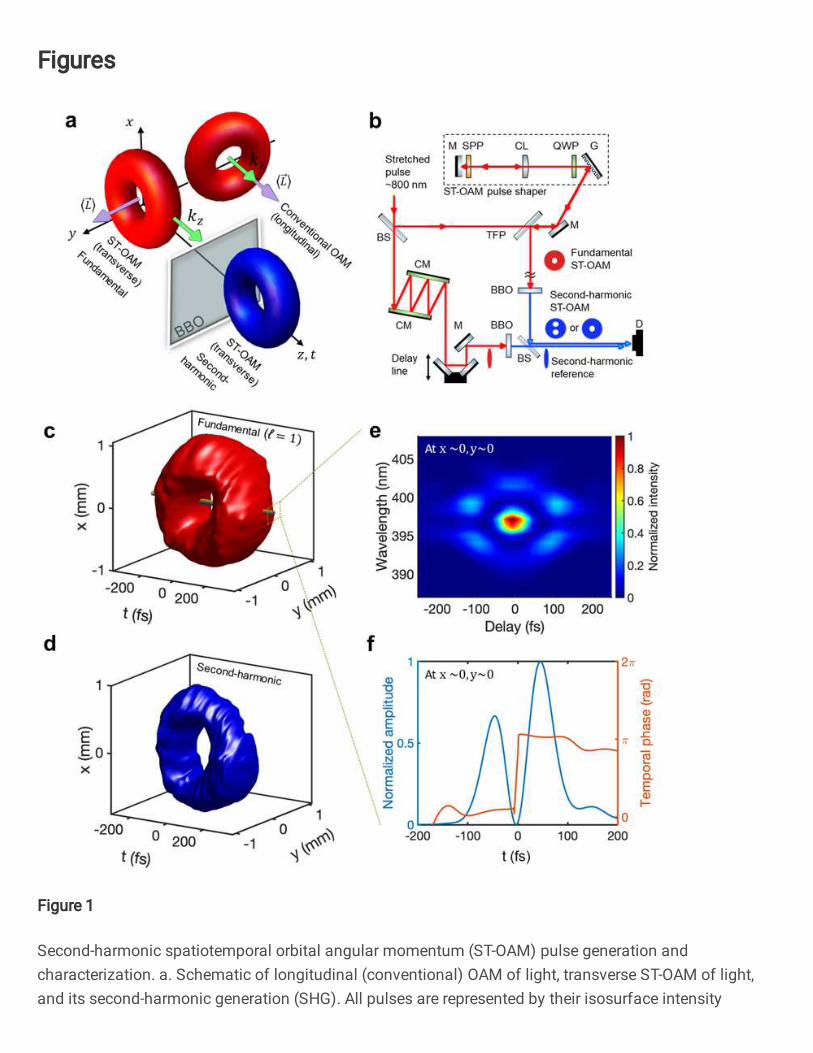
Fig.1 | Second-harmonic spatiotemporal orbital angular momentum (ST-OAM) pulse generation and characterization. a. Schematic of longitudinal (conventional) OAM of light, transverse ST-OAM of light, and its second-harmonic generation (SHG). All pulses are represented by their isosurface intensity profiles. The averaged OAM ⟨𝐿⟩ (purple arrows) in a conventional OAM pulse is parallel to or aligned with the propagation direction 𝑘⃑ (green arrows), and thus named longitudinal OAM, while the averaged OAM in an ST-OAM pulse is perpendicular to the propagation direction and thus named transverse OAM. b. In the experiment, fundamental ST-OAM pulses of topological charge ℓ =1 are generated by a custom pulse shaper. The pulses carry an azimuthal spatiotemporal phase swirl structure in the x-z plane, parallel to the beam propagation direction along the z-axis. Second-harmonic ST-OAM pulses are generated in a BBO crystal and then characterized by interference with a reference Gaussian pulse. c. Experimentally reconstructed 3D intensity isosurface profile of the fundamental ST-OAM pulse and its second-harmonic shown in d. The intensity profile shows a singularity structure in space and time at the center. The center part of the fundamental ST-OAM pulse (indicated by the brown bar) was experimentally sampled and charactered by a FROG setup, where the measured FROG trace and the reconstructed temporal electric field envelope and the temporal phase are shown in e and f, respectively. M: mirror; DM: dichroic mirror; CM: chirped mirror; CL: cylindrical lens; BS: beam splitter; TFP: thin film polarizer; QWP: quarter wave plate; SPP: spiral phase plate; G: grating; BBO: beta barium borate crystal; D: detectors including a beam profiler and a FROG setup.

5  

Results

The generation and measurement of light with ST-OAM and its second-harmonic. The

generation of ST-OAM pulsed beams is depicted in Fig. 1b. A fundamental pulse at central

wavelength λ = 800 nm from a Ti:Sapphire amplifier is sent to a custom ST-OAM pulse shaper to

generate light with ST-OAM of ℓ = 1 (see Methods). Unlike conventional OAM beams which can

be characterized by space-based methods such as fork hologram19, coherent diffractive imaging20,

structured apertures21, ST-OAM pulses require a space-time or equivalently space-frequency based

characterization method. Figures 1c and 1d show experimentally measured and reconstructed 3D

intensity isosurface profiles of the fundamental and second-harmonic ST-OAM pulse,

respectively.

Interestingly, we realized that a common frequency-resolved optical gating (FROG) setup

can also be used to measure the spatiotemporal phase structure of an ST-OAM pulse by carefully

placing an entrance pinhole at different positions of the beam and scanning over it. Figures 1e and

1f show a typical FROG trace and its reconstruction from a fundamental ST-OAM pulse of ℓ = 1,

measured at the beam center. In Fig. 1f, the field amplitude envelope reconstruction clearly shows

a double-pulse structure in the time domain, and the retrieved temporal phase shows a clear π phase

jump between the front and rear ends, consistent with the expected 2π phase shift along the azimuth

in the x-t plane and a centered phase singularity. Although doable, a spatially resolved FROG

measurement is tedious with slow throughput and known to have ambiguities on nontrivial time

direction, absolute phase, and temporal shift. Therefore, we used a Mach-Zehnder-like scanning

interferometer to optically gate an ST-OAM pulse to fully characterize an ST-OAM pulse and its

second-harmonic.

6  

Briefly, a long, 800-nm fundamental, ST-OAM pulse of ~500 fs of ℓ = 1 was interfered

with a short, 800-nm fundamental, Gaussian reference pulse of ~45 fs to form interference fringes.

These fringes characterize the portion of the ST-OAM pulse gated by the >10x shorter reference

pulse. By scanning the time delay, the spatiotemporal profile of the ST-OAM pulse can be

reconstructed computationally from the delay-dependent fringes, where each delay is a time frame

of the reconstruction (See Methods). Some representative fringe patterns of ST-OAM pulses are

shown in Fig. 2, with two black markers added to each time frame as a visual guide to the eye to

observe the fringe shift. The discontinuous phase jump (or phase dislocation) around the

singularity happens close to delay zero. When the reference pulse was scanned towards the ST-

OAM phase singularity (-300 to 0 fs), the fringes are first tilted, and then shifted by a π phase

difference at the center of the singularity. When the reference pulse was scanned away (0 to 300

fs), the fringes become straight again, but the upper and lower fringes were shifted by one fringe.

Such a fringe shift is a feature of an ST-OAM pulse of ℓ = 1. The reconstructed spatiotemporal

amplitude and phase of the fundamental ST-OAM pulse are shown in Fig. 2a-c, based on the fringe

data shown in Fig. 2d. Figure 2a is the amplitude envelope, 2b is the phase, and 2c is a complex

field representation where the amplitude and phase are represented by brightness and hue,

respectively. Our experimentally reconstructed spatiotemporal profiles clearly confirm the

generation of a vortex-shaped ST-OAM pulse with a 2π azimuthal phase swirl in space and time. 

7  

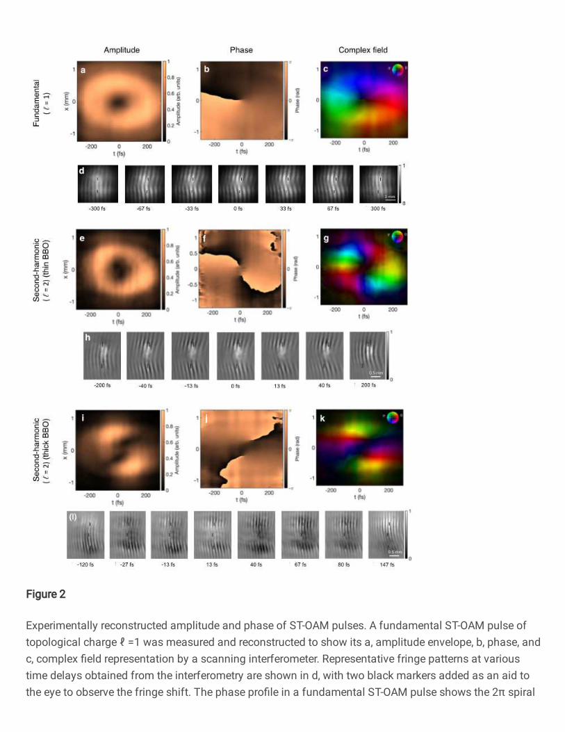
Fig.2 | Experimentally reconstructed amplitude and phase of ST-OAM pulses. A fundamental ST-OAM pulse of topological charge ℓ =1 was measured and reconstructed to show its a, amplitude envelope, b, phase, and c, complex field representation by a scanning interferometer. Representative fringe patterns at various time delays obtained from the interferometry are shown in d, with two black markers added as an aid to the eye to observe the fringe shift. The phase profile in a fundamental ST-OAM pulse shows the 2π spiral phase accumulation on traversing a closed spatiotemporal path around the singularity. A second-harmonic ST-OAM pulse generated by a thin BBO crystal was measured and reconstructed using the same method to show its d, amplitude envelope, e, phase, f, complex field representation, and g. representative fringe patterns. The results show that the spatiotemporal topological charge is also doubled after frequency doubling, evidenced by the 4π phase accumulation. The SHG with topological charge ℓ =2 indicates the conservation of ST-OAM. A second-harmonic ST-OAM pulse was also generated by a thick BBO crystal and measured in h, amplitude envelope, i, phase, j, complex field representation, and k, representative fringe patterns. The OAM is still conserved in this case, but the two singularities are generated and separated further in both space and time, comparing to the case in a thin BBO crystal. The color wheels for complex field representation are shown at the top right corners of a, g, k, where amplitude and phase are represented by brightness and hue, respectively.

8  

Second-harmonic fields were generated by sending the fundamental pulses through

individual BBO crystals on two arms of a similar interferometer. Therefore, we obtained a long,

400-nm second-harmonic, ST-OAM pulse of an unknown, to-be-determined charge ℓ, and a short,

400-nm second-harmonic, Gaussian reference pulse to form interference fringes. A second-

harmonic ST-OAM pulse generated by a thin BBO crystal (20 µm in thickness) is experimentally

reconstructed and shown in Fig. 2e, 2f, and 2g. Figure 2h shows the fringe patterns used for

reconstruction, also with black markers added as visual aids, where we can see the upper and the

lower parts of the pattern are shifted by two fringes, indicating a 4π phase shift when moving

across the singularity. The amplitude envelope profile of the second-harmonic pulse still looks

close to a simple vortex shape, which shares the same topology with the fundamental ST-OAM

pulse: a torus of genus close to one. Although the reconstructed phase profile shows two

singularities, they are almost overlapped in the time domain and slightly dislocated in space by

only ~200 µm, approximating a single phase singularity with 4π azimuthal spiral phase in space-

time. The small singularity separation can be attributed to a slight offset of the laser central

wavelength to the design SPP wavelength, and/or a slight amount of astigmatism of the initial

Gaussian beam. Also, the generation of the fundamental spatial OAM beams are far from perfect

inside the pulse shaper—they are generated slightly off the Fourier plane of the 4-f pulse shaper

because we relied on the beam double passing through the same SPP by retroreflection.

The 4π spiral phase we observed indicates that the second-harmonic ST-OAM pulse has a

confirmed spatiotemporal topological charge of ℓ = 2 after frequency doubling. Therefore, we

established a nonlinear scaling rule and uncovered that the spatiotemporal angular momentum is

conserved during an SHG process.

9  

Spatiotemporal astigmatism and modal analysis. We also investigated a case with

strong spatiotemporal astigmatism by generating second-harmonic ST-OAM pulses using a thick

(1 mm) BBO crystal, as shown in Figs. 2i, j, and k. Unlike the thin BBO case, the second-harmonic

pulse from a thick BBO crystal has a different topology in the pulse profile – there are two

amplitude holes (two phase singularities) close to the center with two outer lobes —  a case

resembling a torus of genus two. The phase profile in Fig. 2j shows two phase singularities with a

2π spiral phase individually, giving rise to a 4π accumulated phase. This again demonstrates ST-

OAM conservation in an SHG process, although the topology is not conserved. The two phase

singularities are dislocated in both time, by ~50 fs, and in space, by ~500 µm. We note that this

separation is recently predicted and presented in a simulation22. Such separation of phase

singularities in the x-t plane can also be observed directly from the fringe patterns in Fig. 2l, where

the upper, middle, and lower parts of the pattern are shifted at various time and spatial locations.

The use of a thicker BBO crystal leads to spatiotemporal astigmatism including phase mismatch

and group velocity mismatch. The phase mismatch narrows the frequency conversion bandwidth

and the group velocity mismatch stretches the second-harmonic pulse duration. Consequently, the

second-harmonic ST-OAM pulses are distorted in space and time, causing a change in topology

of the vortices.

10  

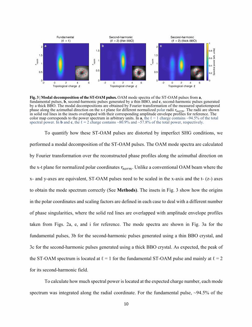
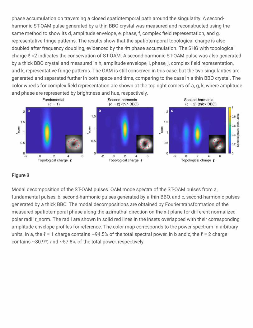
Fig. 3 | Modal decomposition of the ST-OAM pulses. OAM mode spectra of the ST-OAM pulses from a, fundamental pulses, b, second-harmonic pulses generated by a thin BBO, and c, second-harmonic pulses generated by a thick BBO. The modal decompositions are obtained by Fourier transformation of the measured spatiotemporal phase along the azimuthal direction on the x-t plane for different normalized polar radii 𝑟 . The radii are shown in solid red lines in the insets overlapped with their corresponding amplitude envelope profiles for reference. The color map corresponds to the power spectrum in arbitrary units. In a, the ℓ = 1 charge contains ~94.5% of the total spectral power. In b and c, the ℓ = 2 charge contains ~80.9% and ~57.8% of the total power, respectively.

 To quantify how these ST-OAM pulses are distorted by imperfect SHG conditions, we

performed a modal decomposition of the ST-OAM pulses. The OAM mode spectra are calculated

by Fourier transformation over the reconstructed phase profiles along the azimuthal direction on

the x-t plane for normalized polar coordinates 𝑟 . Unlike a conventional OAM beam where the

x- and y-axes are equivalent, ST-OAM pulses need to be scaled in the x-axis and the t- (z-) axes

to obtain the mode spectrum correctly (See Methods). The insets in Fig. 3 show how the origins

in the polar coordinates and scaling factors are defined in each case to deal with a different number

of phase singularities, where the solid red lines are overlapped with amplitude envelope profiles

taken from Figs. 2a, e, and i for reference. The mode spectra are shown in Fig. 3a for the

fundamental pulses, 3b for the second-harmonic pulses generated using a thin BBO crystal, and

3c for the second-harmonic pulses generated using a thick BBO crystal. As expected, the peak of

the ST-OAM spectrum is located at ℓ = 1 for the fundamental ST-OAM pulse and mainly at ℓ = 2

for its second-harmonic field.

To calculate how much spectral power is located at the expected charge number, each mode

spectrum was integrated along the radial coordinate. For the fundamental pulse, ~94.5% of the

11  

total spectral power is located at ℓ = 1 (Fig. 3a). For the second-harmonic pulses generated using

a thin BBO crystal in Fig. 3b, the majority (~80.9%) of the total power is at ℓ = 2 (Fig. 3b),

reflecting the conservation of ST-OAM in the SHG process. However, in the case of a thick BBO

crystal, we observed severe degradation or increased impurity of the modal spectrum, where only

~57.8% of the total power is at ℓ = 2 and a significant DC peak appears (Fig. 3c). This result

indicates that the second-harmonic ST-OAM field is distorted after the generation and propagation

through the thicker crystal due to spatiotemporal astigmatism.

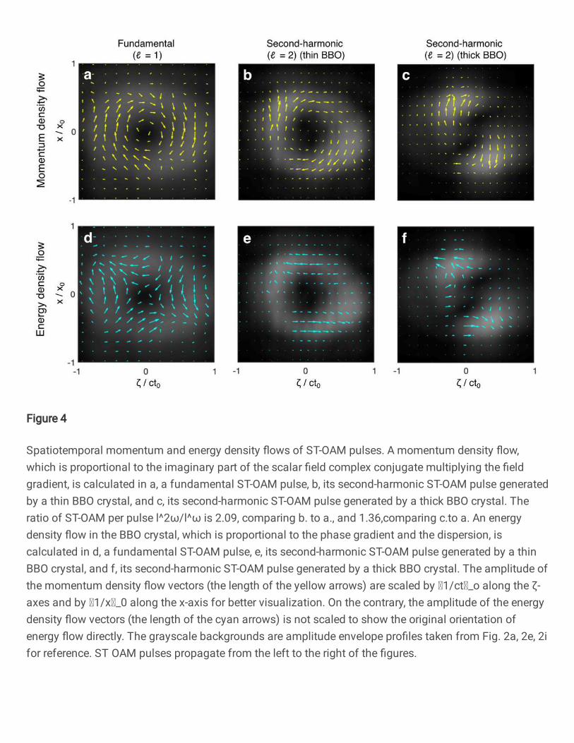
Fig.4 | Spatiotemporal momentum and energy density flows of ST-OAM pulses. A momentum density flow, which is proportional to the imaginary part of the scalar field complex conjugate multiplying the field gradient, is calculated in a, a fundamental ST-OAM pulse, b, its second-harmonic ST-OAM pulse generated by a thin BBO crystal, and c, its second-harmonic ST-OAM pulse generated by a thick BBO crystal. The ratio of ST-OAM per pulse ℓ /ℓ is 2.09, comparing b. to a., and 1.36, comparing c. to a. An energy density flow in the BBO crystal, which is proportional to the phase gradient and the dispersion, is calculated in d, a fundamental ST-OAM pulse, e, its second-harmonic ST-OAM pulse generated by a thin BBO crystal, and f, its second-harmonic ST-OAM pulse generated by a thick BBO crystal. The amplitude of the momentum density flow vectors (the length of the yellow arrows) are scaled by 1/𝑐𝑡 along the 𝜁-axes and by 1/𝑥 along the x-axis for better visualization. On the contrary, the amplitude of the energy density flow vectors (the length of the cyan arrows) is not scaled to show the original orientation of energy flow directly. The grayscale backgrounds are amplitude envelope profiles taken from Fig. 2a, 2e, 2i for reference. ST OAM pulses propagate from the left to the right of the figures.

12  

The momentum and energy density flow of second-harmonic ST-OAM of light. We next

investigated the momentum and energy density flow of the fundamental and its second-harmonic

ST-OAM pulses to better understand the SHG process including spatiotemporal astigmatism.

Given a scalar field 𝐸 𝐸 𝑒 , the momentum density flow is defined by �⃗� Im 𝐸∗𝛻𝐸 .23 Such

momentum density flow can be further used to calculate a single quantity, ST-OAM per

pulse ℓ (see Methods). Adopting this definition, Figs. 4a-4c show our experimentally measured

“spatiotemporal” momentum density flows for a fundamental pulse in 4a, and its second-harmonic

pulse generated using a thin and a thick BBO crystal in 4c and 4b. respectively. The amplitude of

the momentum density flows |�⃗�|, the length of the yellow arrows) are scaled by 1/𝑐𝑡 and by 1/𝑥

in the horizontal and vertical axes for a better visualization.

The momentum density flows of a fundamental ST-OAM pulse follow the gradient of the

phase and form a vortex around the singularity. For a second-harmonic ST-OAM pulse in a thin

BBO crystal, the momentum density flows are no longer uniformly distributed, but they still form

a vortex. In this case, we obtain the ratio of ST-OAM per pulse ℓ /ℓ 2.09, the scenario of a

perfect SHG process. However, for case in a thick BBO, the momentum density flows are

redistributed following the distorted amplitude profile, resulting in the reduced ratio ℓ /ℓ 1.36. The smaller ST-OAM per pulse ratio is consistent with the appearance of a significant DC

peak in the modal spectrum in Fig. 3c, similarly reflecting the degradation and the reduced mode

purity due to spatiotemporal astigmatism in a thick crystal.

To further understand the physical mechanism responsible for this astigmatism, we

calculated the energy density flow in our ST-OAM pulses. The spatiotemporal energy density flow

can be written as 𝚥 E ∇𝜓 GVD 𝜕𝜓/𝜕𝜁 𝜁 /k, following references8,10, where GVD is the

dimensionless group velocity dispersion of the material. In Fig. 4d-4f, the amplitude of the energy

13  

density flows (|𝚥|⃗, the length of the cyan arrows) are presented without rescaling, so we can observe

the energy flow directly. In a fundamental ST-OAM pulse, the energy flows form a saddle-shaped

antivortex structure around the singularity, given the positive GVD at this wavelength for BBO.

As a fundamental ST-OAM pulse propagates through a thin BBO crystal, the SHG process, as well

as a small amount of dispersion, leads to minor energy redistribution. In the case of a thick BBO

crystal, larger dispersion can significantly reshape the ST-OAM pulses, leading to strong

spatiotemporal astigmatism in the second-harmonic ST-OAM pulse. In Fig. 4d-4f, our calculated

energy density flows in the BBO crystal show a tendency to reshape the ST-OAM pulse into a

two-lobe structure upon continued propagation, resulting in the higher degree of distortion

observed for the pulse emerging from the thick BBO crystal.

Discussion

The conservation of ST-OAM and space-time topological charges. The second harmonic ST-

OAM pulse generated using a thin BBO can be described by a simple theory. In a simple scenario

with perfect phase matching and an undepleted pump approximation, assuming a lossless medium,

the second-harmonic field is proportional to the square of the complex input fundamental field,

namely,

𝐸 𝑥,𝑦, 𝜁 𝐸 𝑒 ℓ , , ∝ 𝐸 𝑥,𝑦, 𝜁 ∝ 𝑒 ℓ ∝ 𝑒 ℓ , [2]

where 𝜁 ≡ 𝑧 v 𝑡 is the space coordinate in the moving reference frame of a pulse traveling with

the group velocity v . The definition of the field follows Eq. 1. As a result, 𝑒ℓ 𝑒 ℓ and we

obtain ℓ 2ℓ , indicating that space-time topological charge doubling when the optical

frequency is doubled. In this scenario, the field profile of the second-harmonic wave should mimic

the fundamental pulse. Because the pulse duration and the beam size of a fundamental pulse can

14  

be shortened and reduced in a perfect SHG process due to its quadratic response, it partially

explains the fact that the second-harmonic ST-OAM pulse shown is thinner as shown in Figs. 1c

and d, and Figs. 2e and c.

It is worth mentioning that in the recent study12, the authors argue that the spatiotemporal

topological charge ℓ, which is associated with the total OAM, includes both intrinsic OAM and

extrinsic OAM. Specifically, the intrinsic part still has OAM in the expression of ℏℓ per photon,

as the conventional OAM of light. The other part expressed as 𝑘 ℏ𝑥, is the extrinsic OAM, which

depends on the reference frame but not the charge ℓ . That is, ℏℓ 𝑖𝑛𝑡𝑟𝑖𝑛𝑠𝑖𝑐 OAM 𝑒𝑥𝑡𝑟𝑖𝑛𝑠𝑖𝑐 OAM ℏℓ 𝑘 ℏ𝑥 [3]

Thus, this expression implies that the ST-OAM of light carries the same amount of intrinsic OAM

as the conventional OAM of light, but with an added, reference-frame dependent term. As a result,

we argue that this viewpoint implicitly suggests and agrees with the conservation of ST-OAM in

an SHG process we observed: in a second-harmonic or N-th harmonic generation process, we thus

get 𝑁ℏℓ 𝑁ℏℓ 𝑘 ℏ𝑥, because the integration of the second term around the phase singularity

and the y-axis vanishes for either fundamental or the harmonic field, regardless of its dependence

(or independence) of the nonlinear conversion. Consequently, this result provides the other

perspective in the SHG and the conservation of ST-OAM of light and agrees with our simple SHG

theory in Eq. 2, given an ideal, phase-matched case.

The nonlinear relationship between the electric field amplitudes of a fundamental and its

second-harmonic field means that the amplitude profile of the ST-OAM pulse changes during

frequency doubling. Beyond the simple scenario, the SHG process is further complicated by

additional factors in addition to phase mismatches, such as group velocity mismatch, intrapulse

group velocity dispersion, absorption or losses, and pump depletion24,25. A rigorous theoretical

15  

study of a final second-harmonic ST-OAM pulse profile must take the above factors into account

and is the subject of further detailed investigation, which is beyond the scope of this manuscript.

Implications and applications of ST-OAM of light and its second-harmonic field. There could

be many potential applications in ST-OAM pulses carrying transverse OAM. Conventional OAM

beams carry spatial wavefront structures and are suitable for spatial domain applications such as

enhanced imaging and novel scatterometry5. ST-OAM pulsed beams could enable new

spatiotemporal applications using its temporal profiles for mechanical and thermal acoustic

manipulation of particles, charges, phonon, or spins—space-time singular optics and its

interactions with matter. For instance, even a simple photoemission or photoionization experiment

using a conventional OAM beam provides a wealth of new phenomena26, so we expect new effects

and potentially new selection rules could be revealed by ST-OAM beams. It has also been

demonstrated that the angular momentum carried by conventional OAM beams can be transferred

to objects, leading to applications such as optical tweezers or spanners27–29. In analogy to this idea,

it is theoretically possible to design a “spatiotemporal optical tweezer or spanner” with ST-OAM

pulses for ultrafast manipulation of particles in both spatial and time domain, including new

applications such as microtexturization of implant surfaces. Other applications based on the unique

space-time momentum and energy density flows could be demonstrated in particle acceleration

using structured spatiotemporal nonlinear wakefields30. Conventional OAM beams also provide a

new degree of freedom in photons that can be utilized for multiplexing in telecommunication and

quantum entanglement –– therefore, we anticipate that the ST-OAM of light provides yet another

degree of freedom that could unveil new routes in multiplexing—with a time domain perspective

added such as phase and time-bin encoding31.

16  

Importantly, our demonstration of the ST-OAM nonlinear conversion and the ST-OAM

conservation shows that a new avenue of secondary sources with ST-OAM can be realized

experimentally in up-converted and likely down-converted electromagnetic waves. For example,

it would be of interest to investigate the stimulated OAM Raman scattering,32 harmonic spin-orbit

angular momentum cascade,33 or entangled photons generated by parametric processes with ST-

OAM pulses. It is also possible that other matter waves such as electron vortex beams or electron

bunches with ST-OAM can be generated through photoelectron generation or other means to

improve accelerator technologies and electron microscopy34.

Conclusion. In summary, we report the first experimental observation of a second-harmonic ST-

OAM pulsed beam and its space-time topological charge conversation during frequency doubling.

The charge of the ST-OAM pulse, corresponding to the space-time spiral phase structure, was

observed to double in the SHG process. Our finding also confirms that the spatiotemporal phase

singularities in an ST-OAM pulse can be interpreted as a new class of space-time topological

charges carrying transverse OAM, the term coined in analogy to the spatial topological charges in

a conventional OAM beam carrying longitudinal OAM—both types of OAM follow the same

charge conservation and scaling rules. We also found that the topological structure of the space-

time phase swirl in a second-harmonic field may not be conserved and an SHG process can

generate additional phase singularities, depending on spatiotemporal astigmatism due to group

velocity mismatch or phase mismatch condition. SHG is the foundation of any nonlinear optics

textbook. Our work thus opens a new avenue of light carrying ST-OAM in nonlinear conversion

and scaling, and it further suggests the possibilities to drive secondary ST-OAM sources from

electromagnetic waves, thermoacoustic waves, to matter waves.  

17  

Methods

ST-OAM pulse generation. A stretched (full width at half maximum pulse duration ~ 500 fs)

optical pulse at a central wavelength ~800 nm from a regenerative Ti:sapphire amplifier at 1 kHz

repetition rate (KMLabs Wyvern HE) was first split into two paths before entering into a

homemade Mach-Zehnder-type scanning interferometer. One path is for generating a short (~45

fs), Gaussian reference pulse, and the other is for generating a long (~500 fs) ST-OAM pulse. The

reference Gaussian pulses were compressed using dispersive chirped mirrors (CM, Ultrafast

Innovations) with multiple bounces to shorten the pulse duration. The ST-OAM pulses were

generated by a custom pulse shaper we designed, consisting of a reflective grating (600

grooves/mm), a cylindrical lens (f = 25 cm), a multi-faceted spiral phase plate (SPP, HoloOr, 16-

steps per phase wrap), and a high-reflectance end mirror for retroreflection. To generate

fundamental ST-OAM pulses of spatiotemporal topological charge ℓ = 1, an SPP with designed

spatial topological charge ℓ = 0.5 at the design wavelength 790 nm was used. Upon a

retroreflection from the end mirror, the pulse passes through the SPP twice and generates the

desired spatial topological charge ℓ . Note that an SPP is a non-reciprocal

optical component and a mirror reflection changes the sign of the ℓ , thus, the double-passing of

the SPP from the opposite direction makes the ℓ charge addition possible, when the two passes

are very close. A Fourier transform in the spectral domain of the pulse shaper converts a spatially

chirped beam with a spatial spiral phase into a pulsed beam with a spatiotemporal spiral phase.

Beta barium borate (BBO) crystals with thickness 20 µm (thin BBO) and 1 mm (thick BBO) cut

and oriented to phase match type-I SHG are used to generate the second-harmonic at 400 nm,

which are placed in the far field from the pulse shaper. The second-harmonic Gaussian reference

pulse was generated by another 200-µm thick type-I SHG BBO crystal. To avoid any distortion

and diffraction of the spatiotemporal phase structure after focusing the pulse, we used a nearly

collimated ST-OAM beam in the SHG process, without additional optics that will cause

astigmatism in space and time35.

The amplitude and phase reconstruction-FROG. Fundamental ST-OAM pulses were first

measured using an SHG frequency-resolved optical gating (FROG) setup (videoFROG,

MesaPhotonics) with an added small aperture to spatially sample the center of the beam. The field

amplitude |𝐸 𝑥 0,𝑦 0, 𝑡 | and the phase 𝛷 𝑥 0, 𝑦 0, 𝑡 were then iteratively

18  

reconstructed using the measured FROG trace. In the FROG measurements, we used a compressed

ST-OAM pulse with a shorter pulse duration for easier implementation in the FROG setup, in

comparison with the longer ST-OAM pulse shown in Fig. 1c. Note that given sufficient spatial

samplings over the beam, a FROG setup can characterize the spatiotemporal field profile of an ST-

OAM pulse, although the procedure is tedious and time consuming. Also, the SHG FROG used

here is known to have ambiguities on nontrivial time direction, absolute phase, and temporal shift.

The amplitude and phase reconstruction-interferometer. Both fundamental and second-

harmonic pulse amplitude |𝐸 | and phase 𝛷 were measured using a Mach-Zehnder-type scanning

interferometer. When scanning the time delay between a short reference pulse and a long ST-OAM

pulse, the reference pulse serves as an optical gating pulse that provides spatial information of both

amplitude and phase at the given time delay. We used 38 delays to reconstruct fundamental ST-

OAM pulses and >50 delays for second-harmonic ST-OAM pulses. To reconstruct the 3D

amplitude profile |𝐸 𝑥,𝑦, 𝑡 |, we first extracted the envelope of the fringe patterns at various time

delays. At each time delay, the fringe envelope was then divided by the amplitude of the reference

beam, which gives the 2D amplitude of the ST-OAM pulse at each delay. By stacking 2D

amplitude profiles at various time delays, a 3D amplitude reconstruction is retrieved. We then used

them to calculate and present 3D intensity isosurface profiles, with 37% energy of the wave

contained in the torus-shaped isosurface, as shown in Fig. 1c & 1d. On the other hand, the 2D

amplitude profiles shown in Fig. 2 are projections along the y-axis of the 3D amplitude profiles on

to the x-t plane, |𝐸 𝑥, 𝑡 |. To reconstruct the phase, we first applied 1D Fourier transform to the

original fringe patterns along the y-axis. By extracting the phase of the AC peak in the Fourier

domain, we obtained a 1D phase profile from each 2D fringe pattern, representing 𝛷 𝑥 at each

time delay. The 2D phase reconstruction is retrieved by stacking 1D profiles at each time delay.

It is worth mentioning that due to the instability of the interferometer, the position of the fringe

patterns can vary shot-to-shot. To overcome this problem, the delay-dependent 1D phase profiles

were numerically shifted by constant phases, which are calculated by the amplitude-weighted least

square method to achieve the best phase continuity (smoothness) in the time domain. Besides, all

phase profiles were subtracted by the same background to minimize linear phases and the trivial

temporal phase 𝑒 is omitted. Both amplitude and phase reconstructions in Fig.2 were further

interpolated for better visualization.

19  

OAM modal decomposition. OAM mode spectra are obtained by calculating the azimuthal

Fourier transform of the measured spatiotemporal phase along the azimuthal direction in the x-t

plane using normalized polar coordinates, 𝑟 𝑥/𝑥 𝑐𝑡/𝑐𝑡 and 𝜙 tan 𝑥/𝑥 / 𝑐𝑡/𝑐𝑡 . To calculate the normalization factors 𝑥 and 𝑡 for normalization, we first defined

the origin of the polar coordinate as the position of the phase singularity (or the midpoint of

multiple singularity positions), corresponding to the central minimum in the amplitude profile.

Then a cross-section of the vortex, including the origin, was plotted along the x-axis and the t-axis.

These cross-sections show two peaks, i.e., the front and rear ends of the wheel. We defined 𝑥 and 𝑡 to be one half of the peak-to-peak separation along the x- and t-axis, respectively. In Fig. 3c,

the scaling factors were inherited from Fig. 3b, since the amplitude profile shown in Fig. 3c is not

in an ideal vortex shape. The spectral resolution is limited to one, a quantized integer for the

spatiotemporal topological charges. The plots are interpolated for smoothness.

Spatiotemporal momentum and energy density flows. The momentum and energy density flows

are calculated based on the reconstructed phase in the x-t plane. The gradient operation is achieved

by numerically calculating the differential of the phase, and applying a moving average to the

resultant vector field to remove high frequency noise. The amplitude of the momentum density

flow vectors |�⃗�|, the length of the yellow arrows in Fig. 4a-4c, are scaled by 1/𝑥 , 𝑥 1.25 𝑚𝑚,

on the x-axes and 1/𝑐𝑡 , 𝑡 300 𝑓𝑠, on the 𝜁-axes for better visualization. On the contrary, the

amplitude of the energy density flow vectors |𝚥|, the length of the cyan arrows in Fig. 4d-4f, are

not scaled to show the original orientation of energy flow directly. The dominant but trivial linear

momentum and energy density flow in the t (or z) direction is removed, respectively. The quantized

charge ℓ is calculated by the 2D “volume” integration of the momentum density flows following

the equation12: ℓ ≡ ℏ 𝑟 𝑃 𝑑𝑉 / 𝐸∗𝐸𝑑𝑉.

Data Availability

The datasets utilized to prepare the data presented in this manuscript are available and free of

charge from the corresponding author under reasonable request.

20  

Reference

1. Coullet, P., GIL, L. & Rocca, F. Optical Vortices. Opt. Commun. 73, 403–408 (1989).

2. Allen, L., Beijersbergen, M. W., Spreeuw, R. J. C. & Woerdman, J. P. Orbital angular

momentum of light and the transformation of Laguerre-Gaussian laser modes. Phys. Rev.

A 45, 31–35 (1992).

3. Curtis, J. E. & Grier, D. G. Structure of Optical Vortices. Phys. Rev. Lett. 90, 4 (2003).

4. Vaziri, A., Pan, J. W., Jennewein, T., Weihs, G. & Zeilinger, A. Concentration of higher

dimensional entanglement: Qutrits of photon orbital angular momentum. Phys. Rev. Lett.

91, 1–4 (2003).

5. B. Wang, M. Tanksalvala, Z. Zhang, Y. Esashi, N. Jenkins, M. Murnane, H. Kapteyn, and

C.-T. L. Coherent Fourier scatterometry using orbital angular momentum beams for defect

detection. Submitted (2020).

6. Padgett, M. J. Orbital angular momentum 25 years on. Opt. Express 25, 11265 (2017).

7. Shen, Y. et al. Optical vortices 30 years on: OAM manipulation from topological charge

to multiple singularities. Light Sci. Appl. 8, (2019).

8. Sukhorukov, A. P. & Yangirova, V. V. Spatio-temporal vortices: properties, generation

and recording. Nonlinear Opt. Appl. 5949, 594906 (2005).

9. Bliokh, K. Y. & Nori, F. Spatiotemporal vortex beams and angular momentum. Phys. Rev.

A 86, 1–8 (2012).

10. Jhajj, N. et al. Spatiotemporal optical vortices. Phys. Rev. X 6, 1–13 (2016).

11. Hancock, S. W., Zahedpour, S., Goffin, A. & Milchberg, H. M. Free-space propagation of

spatiotemporal optical vortices. Optica 6, 1547 (2019).

12. Chong, A., Wan, C., Chen, J. & Zhan, Q. Generation of spatiotemporal optical vortices

with controllable transverse orbital angular momentum. Nat. Photonics 14, 350–354

(2020).

13. Dholakia, K.; Simpson, N. B.; Padgett, M. J.; and Allen, L. Second-harmonic generation

and the orbital angular momentum of light. Phys. Rev. A 54, 3742–3745 (1996).

14. Courtial, J., Dholakia, K., Allen, L. & Padgett, M. J. Second-harmonic generation and the

conservation of orbital angular momentum with high-order Laguerre-Gaussian modes.

Phys. Rev. A 56, 273–276 (1997).

15. Hernández-García, C., Picón, A., San Román, J. & Plaja, L. Attosecond extreme

21  

ultraviolet vortices from high-order harmonic generation. Phys. Rev. Lett. 111, 1–5

(2013).

16. Strohaber, J. et al. Coherent transfer of optical orbital angular momentum in multi-order

Raman sideband generation. Opt. Lett. 37, 3411 (2012).

17. Dorney, K. M. et al. Controlling the polarization and vortex charge of attosecond high-

harmonic beams via simultaneous spin–orbit momentum conservation. Nat. Photonics 13,

123–130 (2019).

18. Rego, L. et al. Generation of extreme-ultraviolet beams with time-varying orbital angular

momentum. Science. 364, (2019).

19. Bazhenov, V. Y., Soskin, M. S. & Vasnetsov, M. V. Screw dislocations in light

wavefronts. J. Mod. Opt. 39, 985–990 (1992).

20. Esashi, Y. et al. Ptychographic amplitude and phase reconstruction of bichromatic vortex

beams. Opt. Express 26, 34007 (2018).

21. Hickmann, J. M., Fonseca, E. J. S., Soares, W. C. & Chávez-Cerda, S. Unveiling a

truncated optical lattice associated with a triangular aperture using light’s orbital angular

momentum. Phys. Rev. Lett. 105, 1–4 (2010).

22. Hancock, S. W., Zahedpour, S. & Milchberg, H. M. Orbital angular momentum

conservation in second- harmonic generation with spatiotemporal optical vortices. Front.

Opt. + Laser Sci. APS/DLS, OSA Tech. Dig. (Optical Soc. Am. 2020), Pap. FM7C.6.

23. Speirits, F. C. & Barnett, S. M. Do waves carrying orbital angular momentum possess

azimuthal linear momentum? Phys. Rev. Lett. 111, 4–6 (2013).

24. Sidick, E., Knoesen, A. & Dienes, A. Ultrashort-pulse second-harmonic generation. I .

Transform-limited fundamental pulses. J. Opt. Soc. Am. B 12, 1704–1712 (1995).

25. Sidick, E., Dienes, A. & Knoesen, A. Ultrashort-pulse second-harmonic generation. II.

Non-transform-limited fundamental pulses Erkin. J. Opt. Soc. Am. B 12, 1713–1722

(1995).

26. Picón, A. et al. Photoionization with orbital angular momentum beams. Opt. Express 18,

3660 (2010).

27. He, H., Friese, M. E. J., Heckenberg, N. R. & Rubinsztein-Dunlop, H. Direct observation

of transfer of angular momentum to absorptive particles from a laser beam with a phase

singularity. Phys. Rev. Lett. 75, 199–202 (1995).

22  

28. Paterson, L. et al. Controlled rotation of optically trapped microscopic particles. Science.

292, 912–914 (2001).

29. MacDonald, M. P. et al. Creation and manipulation of three-dimensional optically trapped

structures. Science. 296, 1101–1103 (2002).

30. Vieira, J. & Mendonça, J. T. Nonlinear laser driven donut wakefields for positron and

electron acceleration. Phys. Rev. Lett. 112, 1–5 (2014).

31. Karimi, E., Marrucci, L., de Lisio, C. & Santamato, E. Time-division multiplexing of the

orbital angular momentum of light. Opt. Lett. 37, 127 (2012).

32. Vieira, J. et al. Amplification and generation of ultra-intense twisted laser pulses via

stimulated Raman scattering. Nat. Commun. 7, 1–7 (2016).

33. Tang, Y. et al. Harmonic spin–orbit angular momentum cascade in nonlinear optical

crystals. Nat. Photonics 14, 658–662 (2020).

34. Verbeeck, J., Tian, H. & Schattschneider, P. Production and application of electron vortex

beams. Nature 467, 301–304 (2010).

35. Chen, J., Wan, C., Chong, A. & Zhan, Q. Subwavelength focusing of a spatio-temporal

wave packet with transverse orbital angular momentum. Opt. Express 28, 18472 (2020).

 

Acknowledgments

The JILA authors gratefully acknowledge funding from an AFOSR MURI (FA9550-16-1-0121).

Author contributions

C.-T.L. conceived the project, G.G. conducted and designed the experiment, and both analyzed

the data. M. M. M. and H. C. K. proposed the research thrust, supervised the research, developed

the generation and measurement capabilities, and applications. All authors contributed to the

discussion and writing of the manuscript. 

23  

Competing interests

M. M. M. and H. C. K. have a financial interest in KMLabs. The other authors declare no

competing financial interests.

Corresponding Authors

Please address all correspondence to Chen-Ting Liao. 

 

Figures

Figure 1

Second-harmonic spatiotemporal orbital angular momentum (ST-OAM) pulse generation andcharacterization. a. Schematic of longitudinal (conventional) OAM of light, transverse ST-OAM of light,and its second-harmonic generation (SHG). All pulses are represented by their isosurface intensity

pro�les. The averaged OAM L (purple arrows) in a conventional OAM pulse is parallel to or alignedwith the propagation direction (k_z ) (green arrows), and thus named longitudinal OAM, while theaveraged OAM in an ST-OAM pulse is perpendicular to the propagation direction and thus namedtransverse OAM. b. In the experiment, fundamental ST-OAM pulses of topological charge ℓ =1 aregenerated by a custom pulse shaper. The pulses carry an azimuthal spatiotemporal phase swirl structurein the x-z plane, parallel to the beam propagation direction along the z-axis. Second-harmonic ST-OAMpulses are generated in a BBO crystal and then characterized by interference with a reference Gaussianpulse. c. Experimentally reconstructed 3D intensity isosurface pro�le of the fundamental ST-OAM pulseand its second-harmonic shown in d. The intensity pro�le shows a singularity structure in space and timeat the center. The center part of the fundamental ST-OAM pulse (indicated by the brown bar) wasexperimentally sampled and charactered by a FROG setup, where the measured FROG trace and thereconstructed temporal electric �eld envelope and the temporal phase are shown in e and f, respectively.M: mirror; DM: dichroic mirror; CM: chirped mirror; CL: cylindrical lens; BS: beam splitter; TFP: thin �lmpolarizer; QWP: quarter wave plate; SPP: spiral phase plate; G: grating; BBO: beta barium borate crystal; D:detectors including a beam pro�ler and a FROG setup.

Figure 2

Experimentally reconstructed amplitude and phase of ST-OAM pulses. A fundamental ST-OAM pulse oftopological charge ℓ =1 was measured and reconstructed to show its a, amplitude envelope, b, phase, andc, complex �eld representation by a scanning interferometer. Representative fringe patterns at varioustime delays obtained from the interferometry are shown in d, with two black markers added as an aid tothe eye to observe the fringe shift. The phase pro�le in a fundamental ST-OAM pulse shows the 2π spiral

phase accumulation on traversing a closed spatiotemporal path around the singularity. A second-harmonic ST-OAM pulse generated by a thin BBO crystal was measured and reconstructed using thesame method to show its d, amplitude envelope, e, phase, f, complex �eld representation, and g.representative fringe patterns. The results show that the spatiotemporal topological charge is alsodoubled after frequency doubling, evidenced by the 4π phase accumulation. The SHG with topologicalcharge ℓ =2 indicates the conservation of ST-OAM. A second-harmonic ST-OAM pulse was also generatedby a thick BBO crystal and measured in h, amplitude envelope, i, phase, j, complex �eld representation,and k, representative fringe patterns. The OAM is still conserved in this case, but the two singularities aregenerated and separated further in both space and time, comparing to the case in a thin BBO crystal. Thecolor wheels for complex �eld representation are shown at the top right corners of a, g, k, where amplitudeand phase are represented by brightness and hue, respectively.

Figure 3

Modal decomposition of the ST-OAM pulses. OAM mode spectra of the ST-OAM pulses from a,fundamental pulses, b, second-harmonic pulses generated by a thin BBO, and c, second-harmonic pulsesgenerated by a thick BBO. The modal decompositions are obtained by Fourier transformation of themeasured spatiotemporal phase along the azimuthal direction on the x-t plane for different normalizedpolar radii r_norm. The radii are shown in solid red lines in the insets overlapped with their correspondingamplitude envelope pro�les for reference. The color map corresponds to the power spectrum in arbitraryunits. In a, the ℓ = 1 charge contains ~94.5% of the total spectral power. In b and c, the ℓ = 2 chargecontains ~80.9% and ~57.8% of the total power, respectively.

Figure 4

Spatiotemporal momentum and energy density �ows of ST-OAM pulses. A momentum density �ow,which is proportional to the imaginary part of the scalar �eld complex conjugate multiplying the �eldgradient, is calculated in a, a fundamental ST-OAM pulse, b, its second-harmonic ST-OAM pulse generatedby a thin BBO crystal, and c, its second-harmonic ST-OAM pulse generated by a thick BBO crystal. Theratio of ST-OAM per pulse l^2ω/l^ω is 2.09, comparing b. to a., and 1.36,comparing c.to a. An energydensity �ow in the BBO crystal, which is proportional to the phase gradient and the dispersion, iscalculated in d, a fundamental ST-OAM pulse, e, its second-harmonic ST-OAM pulse generated by a thinBBO crystal, and f, its second-harmonic ST-OAM pulse generated by a thick BBO crystal. The amplitude ofthe momentum density �ow vectors (the length of the yellow arrows) are scaled by 1/ct_o along the ζ-axes and by 1/x_0 along the x-axis for better visualization. On the contrary, the amplitude of the energydensity �ow vectors (the length of the cyan arrows) is not scaled to show the original orientation ofenergy �ow directly. The grayscale backgrounds are amplitude envelope pro�les taken from Fig. 2a, 2e, 2ifor reference. ST OAM pulses propagate from the left to the right of the �gures.