C H A P T E R 4 Second-Order Equations We are ready to move on to differential equations of higher order. We will start with those of second order. These are especially important since so many of the equations that arise in science and engineering are of second order. In Section 4.2 we will completely solve homogeneous, second-order, linear equations with constant coefficients, and in Section 4.3 we will apply this to the analysis of harmonic motion. We then examine methods of solution for inhomoge- neous equations and apply these methods to the study of forced harmonic motion. 4.1 Definitions and Examples A second-order differential equation is an equation involving the independent vari- able t and an unknown function y along with its first and second derivatives. We will assume it is possible to solve for the second derivative, in which case the equation has the form y = f (t , y , y ). A solution to such an equation is a twice continuously differentiable function y (t ) such that y (t ) = f (t , y (t ), y (t )). Many problems in physics give rise to models that are second-order equations. For example, in the study of motion, almost all models start with Newton’s second law, F = ma . Here we are modeling the displacement x (t ) of a body from some reference point. The derivative of x is the velocity v and the second derivative is the acceleration Polking/Boggess/Arnold: Differential Equations 1/E [Second Pages] 1/25/97 11:35 Page 1 163
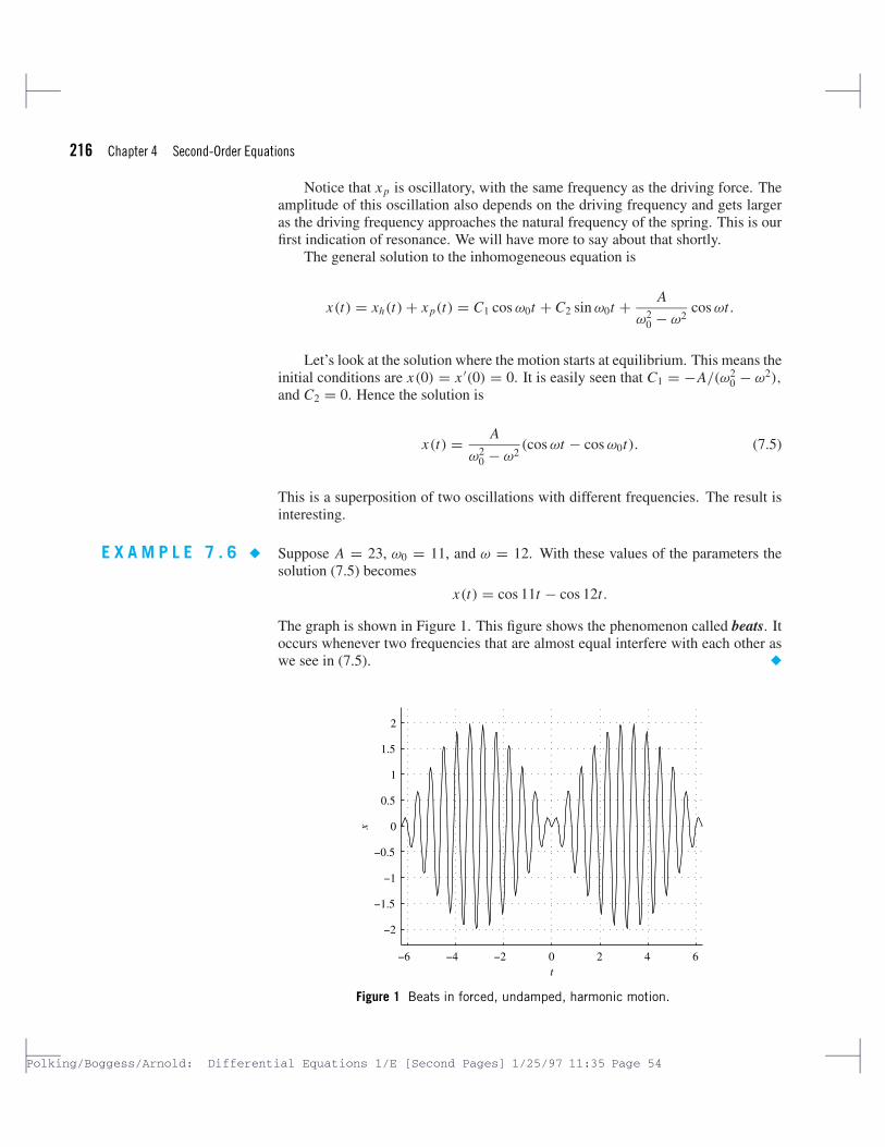
Transcript
CH
AP
TE
R4
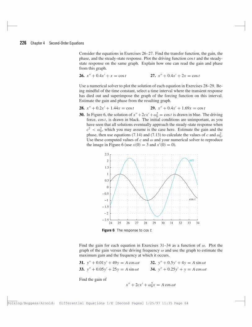
Second-Order Equations
We are ready to move on to differential equations of higher order. We will startwith those of second order. These are especially important since so many of theequations that arise in science and engineering are of second order.
In Section 4.2 we will completely solve homogeneous, second-order, linearequations with constant coefficients, and in Section 4.3 we will apply this to theanalysis of harmonic motion. We then examine methods of solution for inhomoge-neous equations and apply these methods to the study of forced harmonic motion.
4.1 Definitions and ExamplesA second-order differential equation is an equation involving the independent vari-able t and an unknown function y along with its first and second derivatives. We willassume it is possible to solve for the second derivative, in which case the equationhas the form
y′′ = f (t, y, y′).
A solution to such an equation is a twice continuously differentiable function y(t)such that
y′′(t) = f (t, y(t), y′(t)).
Many problems in physics give rise to models that are second-order equations.For example, in the study of motion, almost all models start with Newton’s secondlaw,
F = ma.
Here we are modeling the displacement x(t) of a body from some reference point.The derivative of x is the velocity v and the second derivative is the acceleration
a. The force F acting on the body is usually a function of time t , the displacementx , and the velocity v, or F = F(t, x, v). Thus Newton’s second law gives us thedifferential equation
md2x
dt2= F(t, x, dx/dt),
an equation of second order. We will discuss an important example in this section.
Linear equationsWe will spend most of our time discussing linear equations. These have the specialform
y′′ + p(t)y′ + q(t)y = g(t). (1.1)
The coefficients p, q, and g can be arbitrary functions of the independent variablet , but y, y′, and y′′ must all appear to first order. This means we do not allowproducts of these to occur, nor any powers higher than 1, nor any complicated func-tions like cos y′. For example, when the coefficients p and q are positive constants,equation (1.1) is the equation for the harmonic oscillator, which we will derive laterin this section. On the other hand, the equation for the angular displacement of apendulum bob is
θ ′′ + k sin θ = 0.
Because of the sin θ term this equation is nonlinear.The function g(t) on the right of equation (1.1) is called the forcing term. This
is because in physical systems such a term usually arises from an external force. Forexample, such is the case in the equation of the harmonic oscillator. If the forcingterm is equal to 0, the resulting equation is said to be homogeneous. Thus thehomogeneous equation
y′′ + p(t)y′ + q(t)y = 0. (1.2)
will be called the homogeneous equation associated to (1.1).
An example—the vibrating springAn important example of a second-order differential equation occurs in the model ofthe motion of a vibrating spring. The mathematical principles behind the vibratingspring appear in many areas of science and engineering. The differential equationthat we derive here is the paradigm of oscillatory behavior.
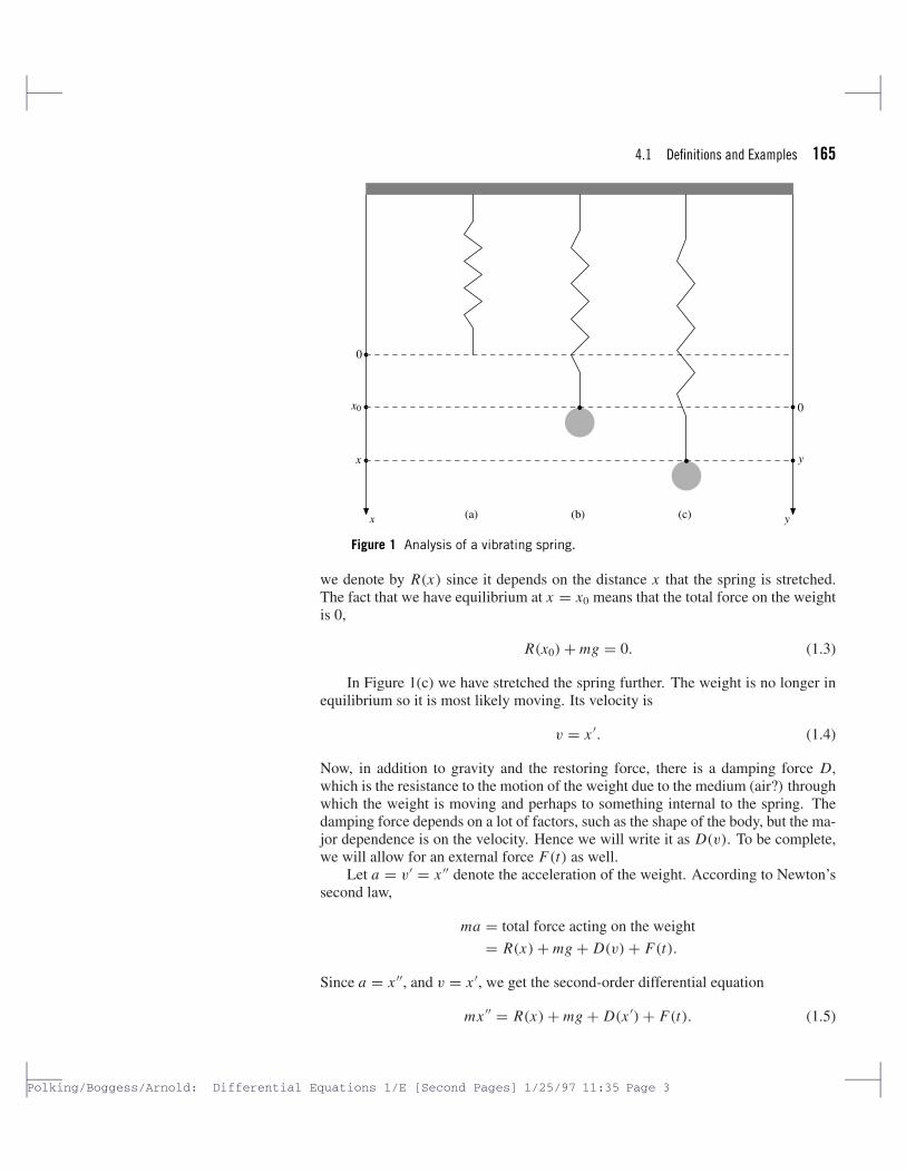
The situation is illustrated in Figure 1. We consider the spring suspended froma beam. In Figure 1(a) we see the spring with no mass attached. It is assumed tobe in equilibrium, so there is no motion. This is called the spring equilibrium. Theposition of the bottom of the spring is the reference point from which we measuredisplacement, so it corresponds to x = 0. We will orient our measurements bymaking x positive below the spring equilibrium.
In Figure 1(b) we have attached a weight of mass m to the spring. This weighthas stretched the spring until it is once more in equilibrium at x = x0. This is calledthe spring-mass equilibrium. At this point there are two forces acting on the mass.There is the force of gravity mg, and there is the restoring force of the spring, which
Delete homogeneous, leaving only "equation" on this line.
4.1 Definitions and Examples 165
x
x
x0
0
y
y
0
(a) (b) (c)
Figure 1 Analysis of a vibrating spring.
we denote by R(x) since it depends on the distance x that the spring is stretched.The fact that we have equilibrium at x = x0 means that the total force on the weightis 0,
R(x0) + mg = 0. (1.3)
In Figure 1(c) we have stretched the spring further. The weight is no longer inequilibrium so it is most likely moving. Its velocity is
v = x ′. (1.4)
Now, in addition to gravity and the restoring force, there is a damping force D,which is the resistance to the motion of the weight due to the medium (air?) throughwhich the weight is moving and perhaps to something internal to the spring. Thedamping force depends on a lot of factors, such as the shape of the body, but the ma-jor dependence is on the velocity. Hence we will write it as D(v). To be complete,we will allow for an external force F(t) as well.
Let a = v′ = x ′′ denote the acceleration of the weight. According to Newton’ssecond law,
ma = total force acting on the weight
= R(x) + mg + D(v) + F(t).
Since a = x ′′, and v = x ′, we get the second-order differential equation
To discover the form of the restoring force we resort to experimentation. Formany springs, it turns out that the restoring force is proportional to the displacement.This experimental fact is referred to as Hooke’s law. It says that
R(x) = −kx . (1.6)
We use the minus sign because the restoring force is acting to decrease the displace-ment, and this allows us to say that the spring constant k is positive. It is importantto realize that Hooke’s law is an experimental fact. There are some springs for whichit is not true, even for small displacements. Test it for a bungee cord, for example.Furthermore, for any spring Hooke’s law is valid only for small displacements. As-suming Hooke’s law, (1.5) becomes
mx ′′ = −kx + mg + D(x ′) + F(t). (1.7)
Assuming, for the moment, that there is no external force and that the weight isat spring-mass equilibrium where x = x0, and x ′ = x ′′ = 0, then the damping forceis D = 0, and we have (see (1.3))
0 = R(x0) + mg = −kx0 + mg or mg = kx0. (1.8)
E X A M P L E 1 . 9 � In an experiment, a 4 kg weight is suspended from a spring. The displacement ofthe spring-mass equilibrium from the spring equilibrium is measured to be 49 cm.What is the spring constant?
This example will give us an opportunity to discuss units. We will use theInternational System, in which the unit of length is the meter (abbreviated m),that of time is the second (abbreviated s), and the unit of mass is the kilogram(abbreviated kg). Other units are derived from these. For example, the unit forvelocity is m/s, and that for acceleration is m/s2. Thus, the acceleration due togravity near the earth is g = 9.8 m/s2. According to this system, the unit for forceis kg·m/s2, but this is called a Newton (abbreviated N).
We can determine the spring constant in our example by solving (1.8) for k,
k = mg
x0.
According to our data, the mass m = 4 kg, and x0 = 49 cm = 0.49 m. Usingg = 9.8 m/s2, we find that the spring constant is
k = 4 kg × 9.8 m/s2
0.49 m= 80 kg/s2. �
Using (1.8) to substitute for mg in equation (1.7), it becomes
mx ′′ = −k(x − x0) + D(x ′) + F(t).
This motivates us to introduce the new variable y = x − x0. Notice that y is thedisplacement of the weight from the spring-mass equilibrium (see Figure 1). Sincey′ = x ′ and y′′ = x ′′, our equation becomes
The damping force D(v) always acts against the velocity. Hence we can writeit as
D(v) = −µv, (1.11)
where µ = µ(v) is a non-negative function of the velocity. Again it is an exper-imental fact that for objects of many shapes and for small velocities, the dampingforce is proportional to the velocity. In such cases µ is a nonnegative constant,called the damping constant. Again there are examples when the dependence of Don v is more complicated.
If we use (1.11) in equation (1.10) it becomes
my′′ = −ky − µy′ + F(t) (1.12)
or
my′′ + µy′ + ky = F(t). (1.13)
If µ is a constant, this is a second-order, linear differential equation for the dis-
disp
lace
men
t
2
0 5 10 15 20
1
−2
−1
0
Figure 2 A vibrating spring withno damping.
placement y(t). We can compute the solution numerically. With k = 3, m = 1, nodamping (µ = 0), and no external force (F(t) = 0), a solution is plotted in Figure 2.In Figures 3 and 4, we see the results with damping—in Figure 3 µ = 0.4, and inFigure 4 µ = 4.
Let’s look at the case when the spring is undamped (µ = 0) and unforced(F(t) = 0). Then our equation reduces to
y′′ = − k
my. (1.14)
Can we solve this equation? We will develop systematic methods to solve suchequations later, but for now we can only use our knowledge of calculus. It mighthelp to look at the solution plotted in Figure 2. To solve equation (1.14) we mustfind a function whose second derivative is a negative multiple of itself. When wethink in those terms (and look at Figure 2) we are led to consider the sine and cosine.With a little experimentation we can discover that
disp
lace
men
t 1
2
0 5 10 15 20
−1
0
Figure 3 A vibrating spring withsmall damping.
cos(√
k/m t)
and sin(√
k/m t)
are solutions to (1.14). In fact, direct substitution shows that any function of theform
y(t) = a cos(√
k/m t)
+ b sin(√
k/m t)
(1.15)
where a and b are constants is a solution to (1.14).
disp
lace
men
t
2
1
0 5 100
Figure 4 A vibrating spring withlarge damping.
From (1.15) we see that our solutions are periodic functions. If we introducethe natural frequency
ω0 = √k/m,
the solution can be written as
y(t) = a cos ω0t + b sin ω0t. (1.16)
If
T = 2π/ω0 = 2π√
m/k
cos ω0(t + T ) = cos(ω0t + ω0T ) = cos(ω0t + 2π) = cos(ω0t)
and the same is true for sin ω0(t + T ). Hence y(t + T ) = y(t), so y is periodic andT is the period.
Existence and uniquenessThe existence and uniqueness results for second-order equations are very similar tothose for first-order equations. We will state a result for linear equations, which wewill find quite useful.
THEOREM 1.17 Suppose the functions p(t), q(t), and g(t) are continuous on the interval (α, β). Lett0 be any point in (α, β). Then for any real numbers y0 and y1 there is one and onlyone function y(t) defined on (α, β), which is a solution to
y′′ + p(t)y′ + q(t)y = g(t) for α < t < β,
and satisfies the initial conditions y(t0) = y0 and y′(t0) = y1.
The major difference between this result and the corresponding theorem forfirst-order linear equations in Section 7 of Chapter 2 is that an initial condition isneeded not only for the function y, but also for its derivative y′. It is important tonotice that we can be sure that a solution exists, and furthermore that it exists overthe entire interval where the coefficients are defined and continuous.
Structure of the general solutionWe will use Theorem 1.17 to find the form of the general solution to a homogeneouslinear equation. It is based on the following result, which is the defining feature oflinearity.
PROPOSITION 1.18 Suppose that y1 and y2 are both solutions to the equation
y′′ + p(t)y′ + q(t)y = 0. (1.19)
Then the function y = C1 y1 + C2 y2, is also a solution to (1.19) for any constantsC1 and C2.
Proof We notice that y′ = C1 y′1 + C2 y′
2, and y′′ = C1 y′′1 + C2 y′′
2 . Consequently,by simply rearranging the terms we get
y′′ + py′ + qy = (C1 y′′
1 + C2 y′′2
) + p(C1 y′
1 + C2 y′2
) + q (C1 y1 + C2 y2)
= C1(y′′
1 + py′1 + qy1
) + C2(y′′
2 + py′2 + qy2
)= 0.
As an example, direct substitution will show that y1(t) = e−t and y2(t) = e−2t
are solutions to the linear equation y′′− y′−2y = 0. In light of Proposition 1.18, weknow that any linear combination y(t) = C1e−t + C2e−2t is also a solution. Againthis can be checked by direct substitution.
The general linear combination, y = C1 y1 + C2 y2, of two solutions y1 and y2,contains two arbitrary constants. One might be led to expect that this is the generalsolution. This is often the case, but not always. This will be the content of our maintheorem. However, to state it we need some terminology.
DEFINITION 1.20 Two functions u and v are said to be linearly indepen-dent if neither is a constant multiple of the other. If one is a constant multipleof the other they are said to be linearly dependent.
Thus, the functions u(t) = t and v(t) = t2 are linearly independent. It is truethat v(t) = tu(t), but the factor t is not a constant. On the other hand u(t) = sin tand v(t) = −4 sin t are obviously linearly dependent.
We are going to use Theorem 1.17 to prove the following result, which willprovide us with our solution strategy for homogeneous equations.
THEOREM 1.21 Suppose that y1 and y2 are linearly independent solutions to the equation
y′′ + p(t)y′ + q(t)y = 0. (1.22)
Then the general solution to (1.19) is
y = C1 y1 + C2 y2,
where C1 and C2 are arbitrary constants.
Theorem 1.21 will be proved after some discussion of the result. We will find itadvantageous to define some more terminology.
DEFINITION 1.23 A linear combination of the two functions u and v isany function of the form
w = Au + Bv,
where A and B are constants.
With this definition we can express Proposition 1.18 by saying that a linearcombination of two solutions is also a solution. Theorem 1.21 says that the generalsolution is the general linear combination of the solutions y1 and y2, provided that y1
and y2 are linearly independent. Because of this result we will say that two linearlyindependent solutions form a fundamental set of solutions.
Notice that Theorem 1.21 defines a strategy to be used in solving homogeneousequations. It says that it is only necessary to find two linearly independent solutionsto find the general solution. That is what we will do in what follows.
E X A M P L E 1 . 2 4 � Find a fundamental set of solutions to the equation for simple harmonic motion,
x ′′ + ω2x = 0.
It can be shown by substitution that
x1(t) = cos ωt and x2(t) = sin ωt
are solutions. (See equation (1.14) and what follows.) It is clear that these functionsare not multiples of each other, so they are linearly independent. It follows from
Theorem 1.21 that x1 and x2 are a fundamental set of solutions. Therefore, everysolution to the equation for simple harmonic motion is a linear combination of x1
and x2. �
To prove Theorem 1.21, we need to know a little more about the impact oflinear independence. The best way to determine if two given functions are linearlyindependent is by simple observation. For example, in Example 1.24 it is prettyobvious that cos ωt and sin ωt are not multiples of each other and therefore arelinearly independent. However, we will need a way of making this determination inmore difficult cases. The Wronskian of two functions u and v is defined to be
W (t) = det
(u(t) v(t)u′(t) v′(t)
)= u(t)v′(t) − v(t)u′(t).
The relationship of the Wronskian to linear independence is summed up in the nexttwo propositions.
PROPOSITION 1.25 Suppose the functions u and v are solutions to the linear, homogeneous equation
y′′ + p(t)y′ + q(t)y = 0
in the interval (α, β). Then the Wronskian of u and v is either identically equal tozero on (α, β) or it is never equal to zero there.
Proof To prove this result, we differentiate the Wronskian W = uv′ −vu′. We get
W ′ = u′v′ + uv′′ − v′u′ − vu′′ = uv′′ − vu′′.
Since u and v are solutions to y′′ + py′ + qy = 0, we can solve for their secondderivatives and substitute. We get
W ′ = u(−pv′ − qv
) − v(−pu′ − qu
)= −p(uv′ − vu′)= −pW.
This is a separable first-order equation for W . If t0 is a point in (α, β), the solutionis
W (t) = W (t0)e− ∫ t
t0p(s) ds for α < t < β.
If W (t0) = 0, then W (t) = 0 for α < t < β. On the other hand, if W (t0) �= 0, thenW (t) �= 0, since the exponential term is never zero.
Consider the solutions x1(t) = cos ωt and x2(t) = sin ωt we found in Exam-ple 1.24. The Wronskian of x1 and x2 is
W (t) = x1(t)x ′2(t) − x ′
1(t)x2(t) = ω0 cos2 ω0t + ω0 sin2 ω0t = ω0.
Thus for these two solutions the Wronskian is never equal to zero. This is alwaysthe case for a fundamental set of solutions, as we will prove in the next result.
PROPOSITION 1.26 Suppose the functions u and v are solutions to the linear, homogeneous equation
y′′ + p(t)y′ + q(t)y = 0 (1.27)
in the interval (α, β). Then u and v are linearly dependent if and only if their Wron-skian is identically zero in (α, β).
Proof Suppose first that u and v are linearly dependent in (α, β). Then one ofthem is a constant multiple of the other. Suppose u = Cv. Then u′ = Cv′ as well,so
Conversely, suppose that W (t) = 0 for α < t < β. It remains to show that uand v are linearly dependent. First, if v(t) = 0 for α < t < β, then v = 0u, so uand v are linearly dependent. Suppose, therefore, that v is not identically equal to 0on (α, β). Suppose that v(t1) �= 0. Since v is continuous, there is an interval (c, d)
containing t1 on which v �= 0. On this interval we have
d
dt
u
v= u′v − uv′
v2= −W
v2= 0.
Hence, on the interval (c, d), u/v is equal to a constant C , or u = Cv. In particular,at t1 we have u(t1) = Cv(t1) and u′(t1) = Cv′(t1). By Proposition 1.18 both u andCv are solutions to the differential equation y′′ + py′ + qy = 0. Since they have thesame initial conditions at t1, it follows from Theorem 1.17 that u = Cv everywherein (α, β). Consequently, u and v are linearly dependent.
Let’s restate the results of these two propositions to highlight the points we willneed.
PROPOSITION 1.28 Suppose the functions u and v are solutions to the linear, homogeneous equation
y′′ + p(t)y′ + q(t)y = 0
in the interval (α, β). If W (t0) �= 0 for some t0 in the interval (α, β), then u andv are linearly independent in (α, β). On the other hand, if u and v are linearlyindependent in (α, β), then W (t) never vanishes in (α, β).
Proof If W (t0) �= 0 for some t0 in the interval (α, β), then by Proposition 1.26, uand v cannot be linearly dependent. Hence they are linearly independent.
If u and v are linearly independent in (α, β), then by Proposition 1.26 the Wron-skian is not identically equal to 0. By Proposition 1.25 it is never equal to 0 in (α, β).
Now we are ready to prove Theorem 1.21.
Proof of Theorem 1.21 Suppose that y1 and y2 are linearly independent solutionsto the equation y′′ + py′ + qy = 0, and suppose that y(t) is any solution. We needto find the constants C1 and C2 such that y = C1 y1 + C2 y2. Let t0 be any point in(α, β). We choose the constants so that
However, this determinant will be recognized as the Wronskian W of y1 and y2.Since y1 and y2 are linearly independent, by Proposition 1.28 we know that W (t0) �=0. Therefore we can find C1 and C2 solving (1.29).
We know that y and C1 y1 + C2 y2 are both solutions to the differential equationy′′ + p(t)y′ + q(t)y = 0, and by (1.29) they have the same initial conditions at t0.By the uniqueness part of Theorem 1.17, we have
y(t) = C1 y1(t) + C2 y2(t) for α < t < β.
Initial value problemsLet’s give some thought to formulating the initial value problem for the second-orderequation y′′ = F(t, y, y′). We see in Theorem 1.17 that to determine a solution yuniquely it is necessary to specify both y(t0) and y′(t0). While the theorem appliesonly to linear equations, this is true for all second-order equations.
E X A M P L E 1 . 3 0 � Find the solution to the equation for simple harmonic motion x ′′ + 4x = 0, withinitial conditions x(0) = 4 and x ′(0) = 2.
We know from Example 1.24 that the general solution has the form
x(t) = a cos 2t + b sin 2t,
where a and b are arbitrary constants. Substituting the initial conditions we get
4 = x(0) = a, and 2 = x ′(0) = 2b.
Thus a = 4 and b = 1 and our solution is
x(t) = 4 cos 2t + sin 2t. �
................EXERCISESIn Exercises 1–4, show, by direct substitution, that the given functions y1(t) andy2(t) are solutions of the given differential equation. Then verify, again by directsubstitution, that any linear combination of the two given solutions is also a solution.
1. y′′ − y′ − 6y = 0, y1(t) = e3t , y2(t) = e−2t
2. y′′ + 4y = 0, y1(t) = cos 2t , y2(t) = sin 2t
3. y′′ − 2y′ + 2y = 0, y1(t) = et cos t , y2(t) = et sin t
In Exercises 5–8, use Definition 1.20 to explain why y1(t) and y2(t) are linearlyindependent solutions of the given differential equation. In addition, calculate theWronskian and use it to explain the independence of the given solutions.
y1(t) = t2 and y2(t) = t |t |are linearly independent on (−∞, +∞). Next, show that the Wronskian of thetwo functions is identically zero on the interval (−∞, +∞). Why doesn’t thisresult contradict Proposition 1.26?
10. Show that y1(t) = et and y2(t) = e−3t form a fundamental set of solutions fory′′ + 2y′ − 3y = 0, then find a solution satisfying y(0) = 1 and y′(0) = −2.
11. Show that y1(t) = cos 4t and y2(t) = sin 4t form a fundamental set of solutionsfor y′′ + 16y = 0, then find a solution satisfying y(0) = 2 and y′(0) = −1.
12. Show that y1(t) = e−t cos 2t and y2(t) = e−t sin 2t form a fundamental set ofsolutions for y′′ + 2y′ + 5y = 0, then find a solution satisfying y(0) = −1 andy′(0) = 0.
13. Show that y1(t) = e−4t and y2(t) = te−4t form a fundamental set of solutionsfor y′′+8y′+16y = 0, then find a solution satisfying y(0) = 2 and y′(0) = −1.
14. Unfortunately, Theorem 1.21 does not show us how to find two independent so-lutions. However, there is a technique that can be used to find a second solutionwhen one solution is known.
(a) Show that y1(t) = t2 is a solution of
t2 y′′ + t y′ − 4y = 0. (1.31)
(b) Let y2(t) = vy1(t) = vt2, where v is a yet to be determined functionof t . Note that if y2/y1 = v, and v is nonconstant, then y1 and y2 areindependent. Show that the substitution y2 = vt2 reduces equation (1.31)to the separable equation
5v′ + tv′′ = 0. (1.32)
Solve equation (1.32) for v, form the solution y2 = vt2, then state thegeneral solution of equation (1.31).
Use the technique shown in Exercise 14 to find the general solution of the secondorder equations in exercises 15–18.
John, Is equation correct? y2 = vt2? The equation $y_2 = vt^2$ is correct. JCP
174 Chapter 4 Second-Order Equations
4.2 Second-Order Equations and SystemsA planar system of first-order equations is a set of two first-order differential equa-tions involving two unknown functions. It might be written as
x ′ = f (t, x, y)
y′ = g(t, x, y),
where f and g are functions of the independent variable t and the two unknowns xand y.
There is a close connection between higher-order equations and first-order sys-tems. In this section, we will begin to explore that connection. Then we will exploreways to visualize solutions to second-order equations. One of those ways involvesthe use of the phase plane, which is really a way of visualizing solutions to planarsystems of equations. We will begin a systematic study of first-order systems inChapter 8.
Second-order equations and planar systemsLet’s look again at the second order equation
y′′ = F(t, y, y′). (2.1)
If we introduce a new variable v = y′, then, in terms of v, equation (2.1) can bewritten v′ = F(t, y, v). We see that the functions y and v are related by the systemof first-order equations
y′ = v
v′ = F(t, y, v)(2.2)
If y is a solution to the second-order equation (2.1), and we set v = y′, thenthe pair of functions y and v solve the first-order system (2.2). The converse is alsotrue. If the pair of functions y and v solve the first-order system (2.2), then y isa solution to the second-order equation (2.1). To see this, notice that by the firstequation in (2.2), y′ = v. Differentiating this and using the second equation in (2.2)we get
y′′ = v′ = F(t, y, v) = F(t, y, y′),which is equation (2.1).
Thus the second-order equation (2.1) and the first-order system (2.2) are equiv-alent in the sense that a solution of either leads to a solution of the other. This factis important for two reasons. First, when solving higher-order equations numeri-cally, it is often necessary to solve the equivalent first-order system, since numericalmethods are typically designed only to solve first-order systems. Second, the equiv-alence allows us to study first-order systems and deduce from them results abouthigher-order equations. This procedure will be illustrated when we begin the studyof first-order systems in Chapter 8.
E X A M P L E 2 . 3 � Let’s look first at one of the most important examples, the single, second-order,linear equation. The general such equation has the form
To find an equivalent system we introduce the new variable v = y′. Thensolving (2.4) for y′′ we see that v′ = y′′ = F(t)− p(t)y′ −q(t)y = F(t)− p(t)v −q(t)y. Hence, y and v solve the system
y′ = v
v′ = F(t) − p(t)v − q(t)y. �
Visualization of solutionsThe simplest and most obvious way to visualize a solution to a second-order differ-ential equation is to graph it. We have already seen examples of this in Figures 2, 3,and 4 in Section 4.1.
Sometimes it is of interest to graph both the solution y and its first derivative,which is especially true if the derivative has physical significance, which is oftenthe case in applications. For example, if we are solving for a displacement y, theny′ = v is the velocity. If we are solving for the charge Q on a condenser, then thederivative Q′ = I is the current. In both of these cases it might be of interest to seegraphs of both the solution and its derivative.
0 10 20 30
−2
2
t
y
Figure 1 The graph of thedisplacement.
0 10 20 300
2
t
− 2
Figure 2 The graph of thevelocity.
Let’s use as an example a damped unforced spring. The equation is
my′′ + µy′ + ky = 0.
Let’s use m = 1, µ = 0.4, and k = 3. We will look at the solution y whichsatisfies the initial conditions y(0) = 2 and v(0) = y′(0) = −1. The graph of thedisplacement y alone is shown in Figure 1, and the graph of the velocity alone isin Figure 2. Sometimes it is useful to see both plotted together. This is shown inFigure 3.
Another type of figure that is often useful is the plot of the curve
t → (y(t), v(t))
in the yv-plane. The yv-plane is called the phase plane, and this is called a phaseplane plot. For our example the phase plane plot is shown in Figure 4. Noticehow this curve spirals into the origin. This gives an interesting visual interpretationof the effect of the damping. Missing from a phase plane plot is any indicationof the dependence on t . However, it does show nicely the interplay between thedisplacement and the velocity.
Also illuminating is a three dimensional (3D) plot of the three variables t , y,and v. These can be plotted either of the orders
t → (t, y(t), v(t)) or t → (y(t), v(t), t).
Which is more effective is often a matter of taste. The latter is shown in Figure 5.The 3D plots show the interplay of all three variables. However, some people findthem difficult to understand. Often they become clearer simply by changing theorientation slightly.
Finally, there is the composite plot, shown in Figure 6. In this one figure we seeplots of y and v versus t , the phase plane plot, and the 3D plot. The relationshipsamong all of these become clearer by looking at this figure. The 3D plot is centralto the figure, and it is shown plotted in blue. This curve will be seen to be the sameas the curve in Figure 5. The plot of the displacement y versus t is shown on theback. It is the projection of the 3D plot onto the back panel. Similarly, the plot of
0 2020
30
y
t
2−2−
Figure 5 A 3D plot oft → (y (t ), v (t ), t ).
v versus t is on the right panel, and it too is a projection of the 3D plot. Finally thephase plane plot is shown on the bottom, and, again, it is the projection of the 3Dplot onto the bottom panel.
John, the "v"s in the art are fine; if they look funny on the screen, increase magnification. Betsy
John C Polking
These can be plotted in either of the orders. Insert "in".
John C Polking
This figure looks out of place here. Would it not look better in the margin? I will leave this to you.
4.2 Second-Order Equations and Systems 177
We see that there are many possible ways to represent solutions. In particularsituations, one of these might be much better than the others. There might also bead hoc representations that are better than any of those shown here.
................EXERCISESIn Exercises 1–6, use the substitution v = y′ to write each second-order equation asa system of two first-order differential equations (planar system).
1. y′′ + 2y′ − 3y = 0 2. 4y′′ + 4y′ + y = 0
3. y′′ + 3y′ + 4y = 2 cos 2t 4. y′′ + 2y′ + 2y = sin 2π t
5. y′′ + µ(t2 − 1)y′ + y = 0 6. y′′+cy′−ay+by3 = A cos ωt
7. Sometimes the physical situation aids in the selection of substitution variables.For example, in an LRC circuit, the current is the derivative of the charge. Inthe LRC circuit governed by the equation
L Q′′ + RQ′ + 1
CQ = E(t),
show that the substitution I = Q′ transforms the equation into the planar system
Q′ = I,
I ′ = − R
LI − 1
LCQ + 1
LE(t).
8. In general, when changing a second order equation to a planar system, thechoice of variables for substitution is arbitrary. If
y′′ = 2y′ − 3y + 2 cos 3t,
show that the substitutions x1 = y and x2 = y′ lead to the planar system
x ′1 = x2,
x ′2 = 2x2 − 3x1 + 2 cos 3t.
In Exercises 9–16, you are given the mass, damping, and spring constants of anundriven spring-mass system
my′′ + µy′ + ky = 0.
You are also given initial conditions. Use a numerical solver to(i) provide separate plots of the position versus time (y vs. t) and the velocity
versus time (v vs. t), and(ii) provide a combined plot of both position and velocity versus time, and
(iii) provide a plot of the velocity versus position (v vs. y) in the yv phase plane.In each exercise, choose a viewing window that highlights the important features ofthe solutions.
9. m = 1 kg, µ = 0 kg/s, k = 4 kg/s, y(0) = −2 m, y′(0) = −2 m/s
10. m = 1 kg, µ = 0 kg/s, k = 9 kg/s2, y(0) = 3 m, y′(0) = 2 m/s
11. m = 1 kg, µ = 2 kg/s, k = 1 kg/s2, y(0) = −3 m, y′(0) = −2 m/s
12. m = 4 kg, µ = 4 kg/s, k = 1 kg/s2, y(0) = 3 m, y′(0) = 1 m/s
13. m = 1 kg, µ = 0.5 kg/s, k = 4 kg/s2, y(0) = 2 m, y′(0) = 0 m/s
14. m = 1 kg, µ = 2 kg/s, k = 1 kg/s2, y(0) = −1 m, y′(0) = −5 m/s
15. m = 1 kg, µ = 3 kg/s, k = 1 kg/s2, y(0) = −1 m, y′(0) = −5 m/s
16. m = 1 kg, µ = 0.2 kg/s, k = 1 kg/s2, y(0) = −3 m, y′(0) = −2 m/s
17. Consider carefully the graphs of v and y versus t , pictured in Figure 3.
(a) Why do the peaks of the curve t → v(t) occur where the curve t → y(t)crosses the t-axis? What is the physical significance of this fact?
(b) Why do the peaks of the curve t → y(t) occur where the curve t → v(t)crosses the t-axis? What is the physical significance of this fact?
18. Consider carefully the phase plane plot of the spring-mass system given in Fig-ure 4.
(a) What physical configuration of the spring-mass system is represented bythe points where the solution curve t → (y(t), v(t)) crosses the y-axis?
(b) What physical configuration of the spring-mass system is represented bythe points where the solution curve t → (y(t), v(t)) crosses the v-axis?
(c) What physical significance can be attached to the fact that the solution curvet → (y(t), v(t)) spirals towards the origin with the passage of time?
If your software supports 3D capability, sketch the solution curve t → (y(t), v(t), t)for the spring-mass system with constants and initial conditions given in the indi-cated exercise.
19. Exercise 9 20. Exercise 10
21. Exercise 15 22. Exercise 16
In Exercises 23–28, you are given the inductance, resistance, and capacitance of adriven LRC circuit
L Q′′ + RQ′ + 1
CQ = 2 cos 2t.
You are also given initial conditions. Use a numerical solver to(i) provide separate plots of the charge on the capacitor versus time (Q vs. t) and
the current in the circuit versus time (I vs. t), and(ii) provide a combined plot of both charge and the current versus time, and
(iii) provide a plot of the current versus the charge (I vs. Q) in the Q I phase plane.See Exercise 7 for aid in setting up the system. In each exercise, choose a viewingwindow that highlights the important features of the solutions.
23. L = 1 H, R = 0 �, C = 1 F, Q(0) = −3 C, I (0) = −2 A
24. L = 1 H, R = 0 �, C = 1/4 F, Q(0) = 1 C, I (0) = 2 A
25. L = 1 H, R = 5 �, C = 1 F, Q(0) = 1 C, I (0) = 2 A
John, in 14 and 15, should the -1's be positive 1's? betsy No. John
John C Polking
Exercise 17 should be changed to: \ex Consider carefully the graphs of $v$ and $y$ versus $t$, shown in Figure~\ref{f4.visyv}. \pt Why do the peaks of the of the curve $t\to y(t)$ occur where the curve $t\to v(t)$ crosses the $t$-axis? What is the physical significance of this fact? \pt Do the peaks of the of the curve $t\to v(t)$ occur where the curve $t\to y(t)$ crosses the $t$-axis?
4.3 Linear, Homogeneous Equations with Constant Coefficients 179
26. L = 2 H, R = 4 �, C = 1 F, Q(0) = −1 C, I (0) = −2 A
27. L = 1 H, R = 0.5 �, C = 1 F, Q(0) = 1 C, I (0) = 2 A
28. L = 1 H, R = 0.2 �, C = 1 F, Q(0) = −11 C, I (0) = −1 A
If your software supports 3D capability, sketch the solution curve t → (Q(t), I (t), t)for the LRC circuit with constants and initial conditions given in the indicated exer-cise.
29. Exercise 23 30. Exercise 24
31. Exercise 27 32. Exercise 28
4.3 Linear, Homogeneous Equations with Constant CoefficientsThis a class of equations which we can solve easily. They are equations of the form
y′′ + py′ + qy = 0, (3.1)
where p and q are constants. If p ≥ 0 and q > 0, this is the equation for unforcedharmonic motion, which we will discuss in the next section. We show there that itincludes the equation for the unforced motion of a vibrating spring, and the equationfor the behavior of an RLC circuit.
Remember the solution strategy we devised in the previous section using The-orem 1.21. It is only necessary to find two linearly independent solutions, whichwe call a fundamental set of solutions. The general solution is the general linearcombination of these.
The key ideaThe analogous first-order, linear, homogeneous equation with constant coefficientsis the equation
y′ + px = 0.
This is the exponential equation. It is separable and easily solved. Its general solu-tion is
y(t) = Ce−pt ,
where C is an arbitrary constant.Motivated by the fact that the first-order equation has an exponential solution,
let’s see if we can find an exponential solution to the second-order equation (3.1).We will look for a solution of the type
y(t) = eλt ,
where λ is a constant, as yet unknown. Inserting this function into our differentialequation, we obtain
y′′ + py′ + qy = λ2eλt + pλeλt + qeλt
= (λ2 + pλ + q)eλt .
Since eλt �= 0, we will have solution to 3.1 if and only if
Change "in the previous section" to in Section 4.1.
John C Polking
Change "y' + px" to y' + py
180 Chapter 4 Second-Order Equations
This is called the characteristic equation for the differential equation in (3.1). Thepolynomial λ2 + pλ + q is called the characteristic polynomial for the equation. Aroot of the characteristic equation is called a characteristic root. If λ is a character-istic root, then y = eλt is a solution to the differential equation.
It is illuminating to write the differential equation and its characteristic equationin proximity,
y′′ + py′ + qy = 0,
λ2 + pλ + q = 0.
This indicates clearly how to pass from the differential equation to its characteristicequation.
Since the characteristic equation is a quadratic equation, its roots are given bythe quadratic formula
λ = −p ± √p2 − 4q
2.
Looking at the discriminant p2 − 4q, we see that there are three cases to consider:
1. two distinct real roots if p2 − 4q > 0;
2. two distinct complex roots if p2 − 4q < 0;
3. one repeated real root if p2 − 4q = 0.
We will look at each of these in what follows. Our way will be guided byTheorem 1.21 in Section 1. We know that if we find a fundamental set of solutions,then the general solution is the general linear combination of these. Thus we needto find two linearly independent solutions.
Distinct real rootsIf λ1 and λ2 are distinct real roots of the characteristic equation, then y1 = eλ1t
and y2 = eλ2t are both solutions. Since the roots are not equal, the solutions arenot constant multiples of each other. Hence, they are linearly independent, and byTheorem 1.21 we have the following result.
PROPOSITION 3.3 If the characteristic equation λ2 + pλ + q = 0 has two distinct real roots λ1 and λ2,then the general solution to y′′ + py′ + qy = 0 is
y(t) = C1eλ1t + C2eλ2t ,
where C1 and C2 are arbitrary constants.
The particular solution for an initial value problem can be found by evaluatingthe constants C1 and C2 using the initial conditions.
E X A M P L E 3 . 4 � Find the general solution to the equation
y′′ − 3y′ + 2y = 0.
Find the unique solution corresponding to the initial conditions y(0) = 2 andy′(0) = 1.
4.3 Linear, Homogeneous Equations with Constant Coefficients 181
Letting y = eλt and inserting this into our differential equation, we obtain
0 = y′′ − 3y′ + 2y = (λ2 − 3λ + 2)eλt .
Thus the characteristic equation is
0 = λ2 − 3λ + 2 = (λ − 2)(λ − 1),
with solutions λ1 = 2 and λ2 = 1. According to Proposition 3.3, the generalsolution is
y(t) = C1e2t + C2et . (3.5)
To find the particular solution for the initial conditions y(0) = 2 and y′(0) = 1,we differentiate the general solution,
y′(t) = 2C1e2t + C2et . (3.6)
Then we substitute t = 0 into (3.5) and (3.6) to obtain the system of equations
2 = y(0) = C1 + C2
1 = y′(0) = 2C1 + C2.
The solutions are C1 = −1 and C2 = 3, so the solution to our initial value problemis
y(t) = −e2t + 3et . �
Complex numbersBefore going into complex roots, let’s spend a little time reviewing complex arith-metic. A complex number is one of the form z = x + iy, where x and y are realnumbers. The number i satisfies i2 = −1. In the complex number z = x + iy,
the real number x is called the real part of z and is denoted by x = Re z. The realnumber y is called the imaginary part of z and is denoted by y = Im z.
Complex addition and multiplication satisfy the usual rules for real numbers.For example,
In multiplication it is necessary to use i2 = −1. For example,
(3 + 5i) · (4 − 2i) = 3(4 − 2i) + 5i(4 − 2i)
= 12 − 6i + 20i − 10i2
= 12 + 14i + 10
= 22 + 14i.
The complex conjugate of the complex number z = x + iy is the numberz = x − iy. Notice that conjugation affects only the imaginary part of the complexnumber, replacing the imaginary part with its negative. In particular, we see that
We can solve the two equations z = x + iy and z = x − iy for x and y obtaining
x = Re z = z + z
2and
y = Im z = z − z
2i.
(3.7)
The process of conjugation preserves algebraic combinations. Suppose thatz = x + iy and w = u + iv are complex numbers. Then the following facts areproved directly from the definition of the conjugate.
z + w = z + w
z − w = z − w
zw = z · w( z
w
)= z
w
The absolute value of a complex number z = x + iy is the real number
|z| =√
x2 + y2.
The absolute value of a complex number has many uses. It is also called the magni-tude of the number, and for many purposes that name is highly illuminating. Noticethat
zz = |z|2. (3.8)
Formula (3.8) provides the secret to computing the reciprocal of a complex number.We have
1
z= 1
z· z
z= z
zz= z
|z|2 . (3.9)
For example,1
4 − 3i= 4 + 3i
|4 − 3i |2 = 4 + 3i
25.
Knowing how to compute reciprocals and products, we can also compute quotients.Thus, using (3.9) we have
w
z= w · 1
z= wz
|z|2 .
Other important properties of the absolute value follow most easily from (3.8).If z and w are two complex numbers, then
|zw| = |z||w| and∣∣∣ z
w
∣∣∣ = |z||w| . (3.10)
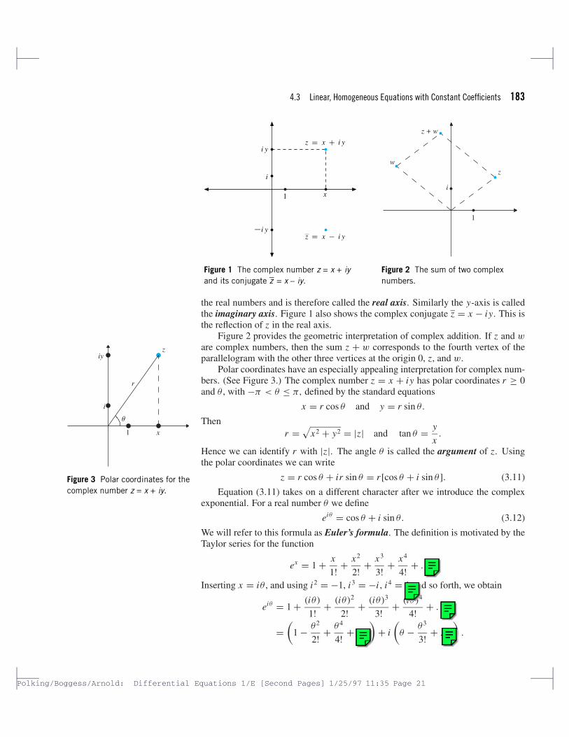
Most people feel more comfortable with complex numbers when they are rep-resented as points in the complex plane. We will identify the complex numberz = x + iy with the point in the plane having cartesian coordinates (x, y). Thisidentification is illustrated in Figure 1. Under this identification the x-axis contains
4.3 Linear, Homogeneous Equations with Constant Coefficients 183
i y
x
z = x + i y
i
1
−i yz = x − i y
Figure 1 The complex number z = x + iyand its conjugate z = x – iy.
1
i
zw
z + w
Figure 2 The sum of two complexnumbers.
the real numbers and is therefore called the real axis. Similarly the y-axis is calledthe imaginary axis. Figure 1 also shows the complex conjugate z = x − iy. This isthe reflection of z in the real axis.
Figure 2 provides the geometric interpretation of complex addition. If z and w
are complex numbers, then the sum z + w corresponds to the fourth vertex of theparallelogram with the other three vertices at the origin 0, z, and w.
Polar coordinates have an especially appealing interpretation for complex num-bers. (See Figure 3.) The complex number z = x + iy has polar coordinates r ≥ 0and θ , with −π < θ ≤ π, defined by the standard equations
x = r cos θ and y = r sin θ.
Thenr =
√x2 + y2 = |z| and tan θ = y
x.
Hence we can identify r with |z|. The angle θ is called the argument of z. Usingthe polar coordinates we can write
z = r cos θ + ir sin θ = r [cos θ + i sin θ ]. (3.11)
Equation (3.11) takes on a different character after we introduce the complex
1
i
z
r
x
iy
θ
Figure 3 Polar coordinates for thecomplex number z = x + iy.
exponential. For a real number θ we define
eiθ = cos θ + i sin θ. (3.12)
We will refer to this formula as Euler’s formula. The definition is motivated by theTaylor series for the function
ex = 1 + x
1! + x2
2! + x3
3! + x4
4! + . . . .
Inserting x = iθ , and using i2 = −1, i3 = −i , i4 = 1 and so forth, we obtain
In this equation and in three following situations the ellipses chould be raised. In TeX notation, use \cdots instead of \dots.
John C Polking
\cdots instead of \dots
John C Polking
\cdots instead of \dots
John C Polking
\cdots instead of \dots
184 Chapter 4 Second-Order Equations
The real part is the Taylor series for cos θ and the imaginary part is the Taylor seriesfor sin θ . Thus eiθ = cos θ + i sin θ .
As a result of Euler’s formula, we can rewrite equation (3.11) as
z = reiθ . (3.13)
This very concise formula expresses the polar coordinates of a complex number.Its usefulness is enhanced after we learn about the full complex exponential and itsproperties. We define the exponential of a complex number by assuming that theaddition formula for the exponential is still valid. The exponential of the complexnumber z = x + iy is defined to be
ez = ex+iy = ex eiy = ex(cos y + i sin y). (3.14)
Thus ex+iy is the complex number with real part ex cos y and imaginary part ex sin y.The complex exponential satisfies all the familiar rules for real exponents. We
set these rules down in the following proposition. The proof is left to the exercises.
PROPOSITION 3.15 The complex exponential satisfies the following properties:
1. ez1+z2 = ez1ez2
2. ez1−z2 = ez1/ez2
3. (ez)r = erz for any real number r
4. ez = ez
5. |ez| = eRe z
6.d
dt{eλt} = λeλt for any complex number λ
Proof As we said previously, the complete proof will be in the exercises. Fornow we will only verify the last property in the special case when λ = i . Thederivative of such a complex valued function is computed by differentiating the realand imaginary parts in the ordinary way. We have
d
dt{eit} = d
dt{cos t + i sin t} by definition of eit
= d
dtcos t + i
d
dtsin t
= − sin t + i cos t
= i(cos t + i sin t)
= ieit .
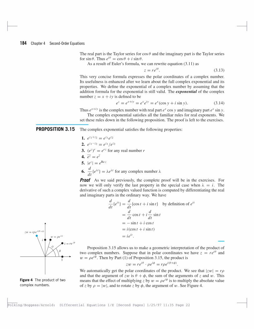
Proposition 3.15 allows us to make a geometric interpretation of the product oftwo complex numbers. Suppose that in polar coordinates we have z = reiθ andw = ρeiφ. Then by Part (1) of Proposition 3.15, the product is
zw = reiθ · ρeiφ = rρei(θ+φ).
We automatically get the polar coordinates of the product. We see that |zw| = rρand that the argument of zw is θ + φ, the sum of the arguments of z and w. Thismeans that the effect of multiplying z by w = ρeiφ is to multiply the absolute valueof z by ρ = |w|, and to rotate z by φ, the argument of w. See Figure 4.
4.3 Linear, Homogeneous Equations with Constant Coefficients 185
Complex rootsIf the roots to the characteristic equation (3.2) are complex, then, since the coeffi-cients of the characteristic polynomial are real, the roots are complex conjugates.They have the form λ = a + ib and λ = a − ib. The corresponding solutions are
z(t) = e(a+ib)t = eat (cos(bt) + i sin(bt)) , and
z(t) = e(a−ib)t = eat (cos(bt) − i sin(bt)) .(3.16)
Clearly the solutions z and z are not multiples of each other, so they are linearlyindependent. Hence using Theorem 1.21, we see that the general solution is
y(t) = C1z(t) + C2z(t). (3.17)
The solutions z and z are complex valued. Such solutions are often preferred (forexample, in circuit analysis). However, we are aiming for real valued solutions.
Notice from (3.16) that z and z are complex conjugates. Written in terms oftheir real and imaginary parts, we have
y1(t) = Re z(t) = eat cos(bt) and y2(t) = Im z(t) = eat sin(bt). (3.19)
From (3.7), we have
y1(t) = 1
2(z(t) + z(t)) and y2(t) = 1
2i(z(t) − z(t)) .
Thus by Proposition 1.18, y1(t) and y2(t), the real and imaginary parts of z(t), aresolutions. Furthermore, these are real valued solutions. Clearly they are not constantmultiples of each other, so they are linearly independent. Hence by Theorem 1.21,they form a fundamental set of solutions, and the general solution can be written as
4.3 Linear, Homogeneous Equations with Constant Coefficients 187
Repeated rootsIf the roots of the characteristic equation (3.2) are repeated, then it becomes
0 = λ2 + pλ + q = (λ − λ1)2
where λ1 is the repeated root. By the quadratic formula,
λ1 =(−p ±
√p2 − 4q
)/2 = −p/2. (3.24)
In order for λ1 to be a double root, we must have p2 −4q = 0. This value of λ givesone solution to the differential equation, namely
y1 = eλ1t .
To use Theorem 1.21, we need to find another solution that is not a constantmultiple of this one. We will use a method of finding the second solution that can beused in many other circumstances when multiple roots give rise to cases that needto be handled separately.
First we point out that in terms of the characteristic roots, the characteristicpolynomial can be written as
λ2 + pλ + q = (λ − λ1)(λ − λ2)
= λ2 − (λ1 + λ2)λ + λ1λ2.
Thus p = −(λ1 + λ2) and q = λ1λ2. This means that the characteristic roots deter-mine the differential equation. The key to our method is to perturb the differentialequation slightly. Instead of looking at our case where λ2 = λ1, we look at theequation where λ2 = λ1 + s, for s a small real number.
The equation with these characteristic roots is
y′′ + (p − s)y′ + (q + λ1s)y = 0, (3.25)
where p = 2λ1 and q = λ21. The characteristic roots for this equation are λ1 and
λ1 + s, so the functions eλ1t and e(λ1+s)t are solutions. In particular, for s �= 0 thefunction
us(t) = 1
s
[e(λ1+s)t − eλ1t
]is a solution to (3.25). Let’s rewrite that as
u′′s + (p − s)u′
s + (q + λ1s)us = 0. (3.26)
We now let s tend to 0 in (3.26). Assuming for the moment that everything makessense, and in particular that u(t) = lims→0 us(t) exists, then in the limit (3.26)becomes
u′′ + pu′ + qu = 0. (3.27)
If everything makes sense, we have discovered a solution to our original equa-tion. Let’s find out what u is by computing the limit
The limit can be computed using either the limit quotient definition of the derivativeor l’Hopital’s rule to get
u(t) = teλ1t .
We suspect that u is actually a solution to (3.27), but that needs verification.There are two ways to do this. The easy way is simply to verify it by direct substi-tution. The harder way is to show that the limit in (3.26) does make sense, and thatthe limit is (3.27). We will leave both of these as exercises.
Thus our second solution is
y2(t) = u(t) = teλ1t .
Since y2 = t y1 and t is not a constant, y2 is not a constant multiple of y1. They arelinearly independent. Theorem 1.21 now gives us the form of the general solution,and we summarize our discussion in the following proposition.
PROPOSITION 3.28 If the characteristic equation λ2 + pλ+ q = 0 has only one double root λ1, then thegeneral solution to y′′ + py′ + qy = 0 is
y(t) = (C1 + C2t) eλ1t ,
where C1 and C2 are arbitrary constants.
The constants C1 and C2 can be found from initial conditions to solve initialvalue problems.
E X A M P L E 3 . 2 9 � Find the general solution to
y′′ − 2y′ + y = 0.
Find the solution corresponding to the initial conditions y(0) = 2 and y′(0) = −1.
The characteristic equation is
0 = λ2 − 2λ + 1 = (λ − 1)2,
so λ = 1 is a double root. Hence, et and tet form a fundamental set of solutions tothis differential equation, and the general solution is
y(t) = C1et + C2tet . (3.30)
To find the solution corresponding to the initial conditions y(0) = 2 andy′(0) = −1, we differentiate y,
y′(t) = C1et + C2tet + C2et . (3.31)
At t = 0, equations (3.30) and (3.31) become
2 = y(0) = C1
−1 = y′(0) = C1 + C2.
This system has solutions C1 = 2 and C2 = −3, so the solution to the initial valueproblem is
4.3 Linear, Homogeneous Equations with Constant Coefficients 189................EXERCISESThe equations in Exercises 1–6 have distinct, real, characteristic roots. Find thegeneral solution in each case.
1. y′′ − y′ − 2y = 0 2. y′′ + 5y′ + 6y = 0
3. y′′ + y′ − 12y = 0 4. 2y′′ − y′ − y = 0
5. 6y′′ + y′ − y = 0 6. 6y′′ + 5y′ − 6y = 0
The equations in Exercises 7–12 have complex characteristic roots. Find the generalsolution in each case.
7. y′′ + y = 0 8. y′′ + 4y = 0
9. y′′ + 4y′ + 5y = 0 10. y′′ + 2y′ + 17y = 0
11. y′′ + 2y = 0 12. y′′ + 2y′ + 2y = 0
The equations in Exercises 13–18 have repeated, real, characteristic roots. Find thegeneral solution in each case.
13. y′′ − 4y′ + 4y = 0 14. y′′ − 6y′ + 9y = 0
15. 4y′′ + 4y′ + y = 0 16. 4y′′ + 12y′ + 9y = 0
17. 16y′′ + 8y′ + y = 0 18. y′′ + 8y′ + 16y = 0
In Exercises 19–28, find the solution of the given initial value problem.
19. y′′ − y′ − 2y = 0, y(0) = −1, y′(0) = 2
20. y′′ − 2y′ + 17y = 0, y(0) = −2, y′(0) = 3
21. y′′ + 25y = 0, y(0) = 1, y′(0) = −1
22. y′′ + 10y′ + 25y = 0, y(0) = 2, y′(0) = −1
23. y′′ − 2y′ − 3y = 0, y(0) = 2, y′(0) = −3
24. y′′ − 4y′ − 5y = 0, y(1) = −1, y′(1) = −1
25. 8y′′ + 2y′ − y = 0, y(−1) = 1, y′(−1) = 0
26. 4y′′ + y = 0, y(1) = 0, y′(1) = −2
27. y′′ + 12y′ + 36y = 0, y(1) = 0, y′(1) = −1
28. y′′ − 4y′ + 13y = 0, y(0) = 4, y′(0) = 0
29. Given that the characteristic equation λ2+pλ+q = 0 has a double root, λ = λ1,show, by direct substitution, that y = teλ1t is a solution of y′′ + py′ + qy = 0.
30. We need to complete some details in the proof of Proposition (3.28). Recallthat we made the following definition.
us(t) = 1
s
[e(λ1+s)t − eλ1t
](3.32)
(a) Use l’Hopital’s rule to show that u(t) = lims→0 us(t) = teλ1t .
(b) Show that u′(t) = lims→0 u′s(t). Again, l’Hopital’s rule is helpful.
(d) Show that the limit of equation (3.26) is equation (3.27), so that u really isa solution to (3.27).
31. Use Euler’s identity to prove that
cos θ = eiθ + e−iθ
2and sin θ = eiθ − e−iθ
2i.
32. Verify equation 3.10. That is, show that if z and w are complex numbers, then
|zw| = |z||w| and∣∣∣ z
w
∣∣∣ = |z||w| .
33. Prove property (1) of Proposition 3.15. The addition formulas for the sine andcosine will be useful.
34. Prove property (2) of Proposition 3.15. This will be easy if you use what youlearned in the previous exercise.
35. Prove property (4) of Proposition 3.15.
36. Prove property (5) of Proposition 3.15.
37. Prove property (6) of Proposition 3.15. Remember that λ = µ+iν is a complexnumber.
4.4 Harmonic MotionIn Section 4.1 we derived the equation for the motion of a vibrating spring. It is (seeequation (1.13))
my′′ + µy′ + ky = F(t), (4.1)
where the constant coefficients are m, the mass, µ, the damping constant, and k, thespring constant, and the function F(t) is an external force.
In Section 3.4 of Chapter 3 we derived differential equations that modeled sim-ple RLC circuits. If the circuit consisted of a resistor of resistance R, a condenser ofcapacitance C , and an inductor of inductance L and had a source voltage E(t), thenthe current I satisfies the equation
Ld2 I
dt2+ R
d I
dt+ 1
CI = d E
dt. (4.2)
The coefficients R, C , and L are all constants.It is interesting to compare equations (4.1) and (4.2). They are almost identical,
differing only in the letters chosen to represent the coefficients and the unknownfunctions. If we compare the coefficients, we see that the inductance L acts like themass m, the resistance R like the damping constant, and the reciprocal of the capac-itance 1/C like the spring constant. Finally, the derivative of the source voltage actslike the external force on the spring.
It is important to keep these analogies in mind. Physically it means that the twophenomena have similar behavior. Mathematically it means that when we discoverfacts about solutions to one of these equations, we also have related facts about the
others. For example, if we have a circuit without resistance (R = 0) and no sourcevoltage, then equation (4.2) simplifies to
Ld2 I
dt2+ 1
CI = 0. (4.3)
This corresponds to the equation for an unforced, undamped spring. Earlier we dis-covered solutions to that equation (see equation (1.15)). Replacing the mass m withthe inductance L , and the spring constant k with the reciprocal of the capacitance1/C , we see that any function of the form
I (t) = a cos(t/√
LC) + b sin(t/√
LC)
is a solution to (4.3).If we divide equations (4.1) and (4.2) by their leading coefficient (L or m), they
become
d2 y
dt2+ µ
m
dy
dt+ k
my = 1
mF(t), and
d2 I
dt2+ R
L
d I
dt+ 1
LCI = 1
L
d E
dt.
If we make the identifications c = µ/2m, ω0 = √k/m, f (t) = F(t)/m, and x = y
in the first equation, or c = R/2L , ω0 = √1/LC, f (t) = (d E/dt)/L , and x = I
in the second, we get the equation
x ′′ + 2cx ′ + ω20 y = f (t), (4.4)
where c ≥ 0 and ω0 > 0 are constants. We will refer to this equation as the equationfor harmonic motion. It includes the vibrating spring and the arbitrary RLC circuit,but there are many other phenomena that lead to this equation.
It is common to use the terminology of the vibrating spring when discussingharmonic motion. In particular, c is called the damping constant, and f is theforcing term.
In this section we will study unforced harmonic motion. This means that f (t) =0 in (4.4), so we will be studying the homogeneous equation
x ′′ + 2cx ′ + ω20x = 0, (4.5)
where c ≥ 0 and ω0 > 0 are constants. This is the type of equation we considered inthe previous section, so we are in a position to analyze unforced harmonic motion.
Simple harmonic motionIn the special case when there is no damping (so c = 0) the motion is called simpleharmonic motion. Equation (4.5) simplifies to
The characteristic roots are λ = ±iω0. According to Proposition 3.20, the generalsolution is
x(t) = a cos ω0t + b sin ω0t, (4.7)
where a and b are constants.If we define T = 2π/ω0, so that ω0T = 2π , then the periodicity of the trigono-
metric functions implies that x(t + T ) = x(t) for all t . Thus, the solution x is itselfperiodic with period T . For this reason, ω0 is called the natural frequency of thespring. We will continue with this terminology even in the damped case.
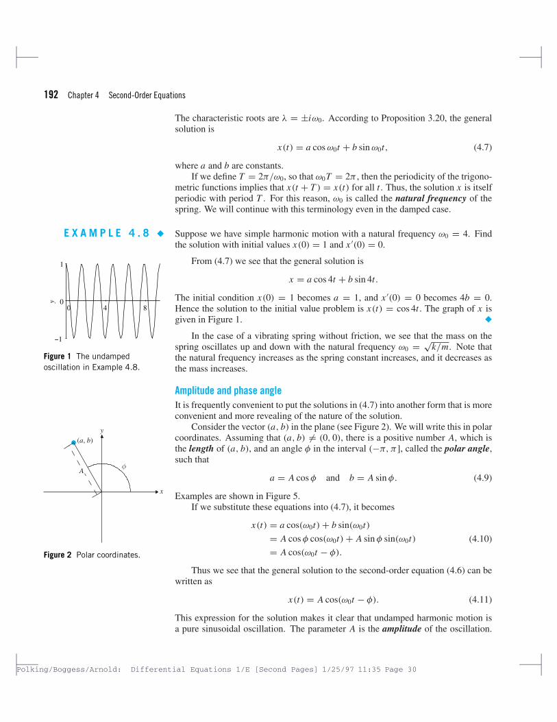
E X A M P L E 4 . 8 � Suppose we have simple harmonic motion with a natural frequency ω0 = 4. Findthe solution with initial values x(0) = 1 and x ′(0) = 0.
From (4.7) we see that the general solution is
0 4 8
−1
0
1
y
Figure 1 The undampedoscillation in Example 4.8.
x = a cos 4t + b sin 4t.
The initial condition x(0) = 1 becomes a = 1, and x ′(0) = 0 becomes 4b = 0.Hence the solution to the initial value problem is x(t) = cos 4t. The graph of x isgiven in Figure 1. �
In the case of a vibrating spring without friction, we see that the mass on thespring oscillates up and down with the natural frequency ω0 = √
k/m. Note thatthe natural frequency increases as the spring constant increases, and it decreases asthe mass increases.
Amplitude and phase angleIt is frequently convenient to put the solutions in (4.7) into another form that is moreconvenient and more revealing of the nature of the solution.
Consider the vector (a, b) in the plane (see Figure 2). We will write this in polar
x
y
A
(a, b)
φ
Figure 2 Polar coordinates.
coordinates. Assuming that (a, b) �= (0, 0), there is a positive number A, which isthe length of (a, b), and an angle φ in the interval (−π, π ], called the polar angle,such that
a = A cos φ and b = A sin φ. (4.9)
Examples are shown in Figure 5.If we substitute these equations into (4.7), it becomes
x(t) = a cos(ω0t) + b sin(ω0t)
= A cos φ cos(ω0t) + A sin φ sin(ω0t)
= A cos(ω0t − φ).
(4.10)
Thus we see that the general solution to the second-order equation (4.6) can bewritten as
x(t) = A cos(ω0t − φ). (4.11)
This expression for the solution makes it clear that undamped harmonic motion isa pure sinusoidal oscillation. The parameter A is the amplitude of the oscillation.
Since the cosine term oscillates between ±1, the limits of the oscillation in (4.11)are ±A. The parameter φ represents the phase of the oscillation. A positive phaseshifts the graph of the cosine to the right. This effect is shown in Figure 3. It canbest be understood by writing (4.11) as
x(t) = A cos
(ω0
(t − φ
ω0
)).
Notice that there are still two undetermined constants in (4.11). Now they are theamplitude A and the phase φ.
This is all very well and good, but it is not very useful unless we can find the
t
x
−A
A
ω00x (t) = A cos ω t
2ω0
x (t) = A cos(ω0t )−
φ
φ
π
Figure 3 The phase angle shiftsthe graph of the cosine
constants A and φ when we know a and b. Equations (4.9) tell us how to compute aand b if we know A and φ. They also can be solved for A and φ. First, if we squareeach equation and add, we get
A2 = a2 + b2 or A =√
a2 + b2. (4.12)
Next, if we divide the second equation by the first, we get
tan φ = b
a. (4.13)
While it is tempting to “solve” this last equation for φ and write φ =arctan(b/a), this would be a mistake. As Figure 4 shows, the arctan takes val-ues between −π/2 and π/2, whereas we know that φ can be any angle between−π and π . The range −π/2 < φ < π/2 corresponds to the points (a, b) wherea = A cos φ > 0. These are points (a, b) in the right half-plane. How do wecompute φ when a < 0?
When (a, b) is in the left half-plane, then (−a, −b) is in the right half-plane,
/2
−
−20 −10 0 10 20
−2
−1
0
1
2y = arctan(x)
π
/2π
Figure 4 The arctangent takesvalues between −π /2 and π /2.
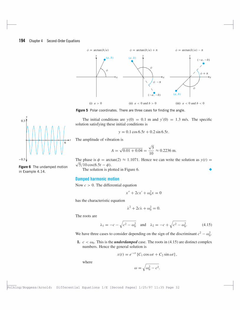
and clearly arctan(b/a) = arctan(−b/ − a). Thus arctan(b/a) is measuring thepolar angle of (−a, −b), which differs by ±π from the polar angle of (a, b) (seeFigure 5). There are three cases depending on the signs of a and b, as shown inFigure 5. Following the angles in Figure 5, we see that the polar angle is given by
φ =
arctan(b/a), if a > 0;arctan(b/a) + π, if a < 0 and b > 0;arctan(b/a) − π, if a < 0 and b < 0.
E X A M P L E 4 . 1 4 � A mass of 4 kg is attached to a spring with a spring constant of k = 169 kg/s2.It is then stretched 10 cm from the spring-mass equilibrium and set to oscillatingwith an initial velocity of 130 cm/s. Assuming it oscillates without damping, findthe frequency, amplitude, and phase of the vibration.
The differential equation is
4y′′ + 169y = 0 or y′′ + 42.25y = 0.
The natural frequency is ω0 = √42.25 = 6.5 and the general solution is
2. c > ω0. This is the overdamped case. Now the roots in (4.15) are distinct and
real. Further, since√
c2 − ω20 <
√c2 = c, we have λ1 < λ2 < 0. The general
solution isx(t) = C1eλ1t + C2eλ2t .
3. c = ω0. This is the critically damped case, and in this case, the root in (4.15) isa double root,
λ = −c.
The general solution is
x(t) = C1e−ct + C2te−ct .
In all of the cases the solution decays to zero as t → ∞ due to the exponentialterm in the solution, and the coefficient c > 0. In the critically damped case, thisfollows since, for r > 0, limt→∞ t/ert = 0 by l’Hopital’s rule.
In the underdamped case the cosine and sine terms cause the solution to oscil-late with frequency ω as it converges to zero. Notice that this frequency is alwayssmaller than the natural frequency of the spring. In the other two cases there is nooscillation.
Let’s look at specific examples of damping phenomena.
E X A M P L E 4 . 1 6 � Consider the spring in Example 4.14 with damping constant µ = 12.8 kg/s. Findthe solution with initial conditions y(0) = 0.1 m and y′(0) = 1.3 m/s.
Since m = 4, k = 169 and µ = 12.8, the differential equation is
The characteristic polynomial λ2 + 3.2λ + 42.25 has roots −1.6 ± i√
42.25 − 1.62
= −1.6 ± 6.3i . Thus, ω = 6.3 and the general solution is
y(t) = e−1.6t(C1 cos 6.3t + C2 sin 6.3t).
For the initial conditions we have
0.1 = y(0) = C1
1.3 = y′(0) = −1.6 C1 + 6.3 C2.
Hence C1 = 0.1 and C2 = 1.46/6.3 ≈ 0.2317. The solution is
y(t) = e−1.6 t(0.1 cos 6.3t + 0.2317 sin 6.3t).
This can also be written as
y(t) = 0.2524e−1.6t cos(6.3t − 1.1634).
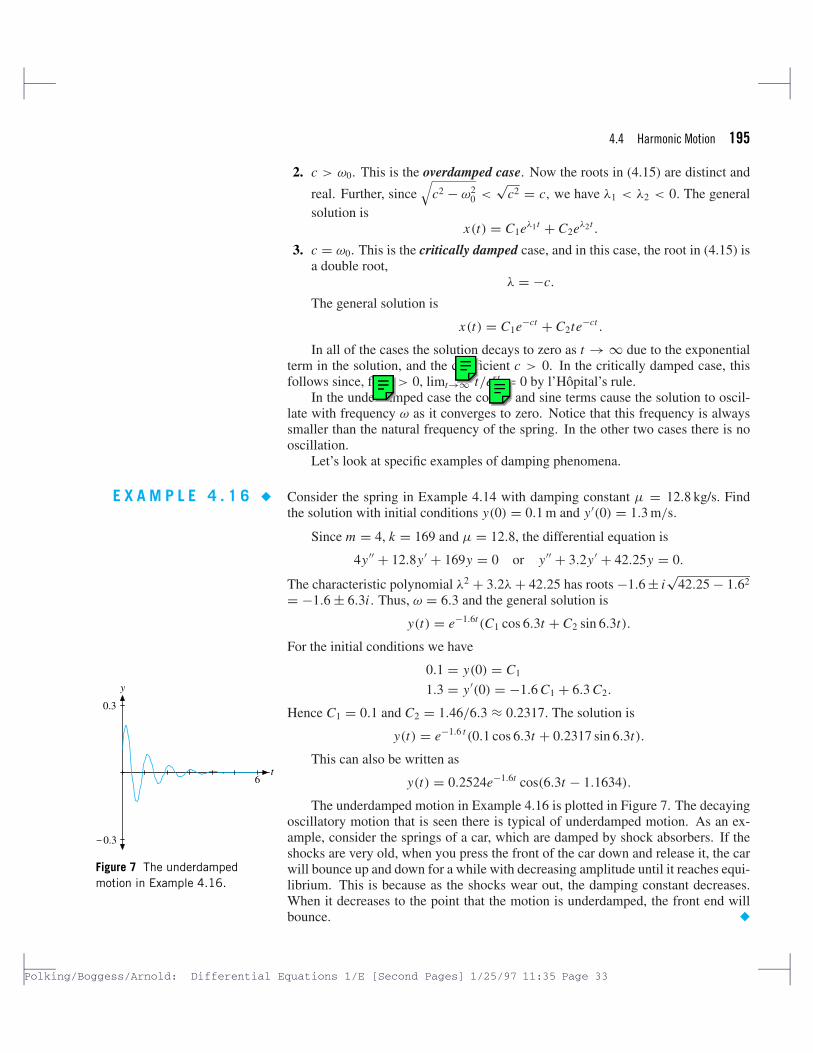
The underdamped motion in Example 4.16 is plotted in Figure 7. The decayingoscillatory motion that is seen there is typical of underdamped motion. As an ex-ample, consider the springs of a car, which are damped by shock absorbers. If theshocks are very old, when you press the front of the car down and release it, the carwill bounce up and down for a while with decreasing amplitude until it reaches equi-librium. This is because as the shocks wear out, the damping constant decreases.
t
y
6
−
0.3
0.3
Figure 7 The underdampedmotion in Example 4.16.
When it decreases to the point that the motion is underdamped, the front end willbounce. �
change "the coefficient $c > 0$" to the fact that $c > 0$
John C Polking
Change $r > 0$ to $c > 0$
John C Polking
Change $t/e^{rt}$ to $t/e^{ct}$
196 Chapter 4 Second-Order Equations
E X A M P L E 4 . 1 7 � Consider the spring in Example 4.14 with damping constant µ = 77.6 kg/s. Findthe solution with initial conditions y(0) = 0.1 m and y′(0) = 1.3 m/s.
Since m = 4, k = 169 and µ = 77.6, the differential equation is
The characteristic polynomial λ2 + 19.4λ + 42.25 has roots
−9.7 ±√
9.72 − 42.25 = −9.7 ± 7.2.
Set λ1 = −16.9 and λ2 = −2.5. This is the overdamped case. The general solutionis
y(t) = C1e−16.9t + C2e−2.5t .
For the initial conditions we have
0.1 = y(0) = C1 + C2
1.3 = y′(0) = −16.9C1 − 2.5C2.
Hence C1 = −31/288, and C2 = 299/1440. The solution is given by
y(t) = − 31
288e−16.9t + 299
1440e−2.5t .
The overdamped motion in Example 4.17 is plotted in Figure 8. Typical of suchbehavior, the displacement decreases to its equilibrium without the oscillation wesee in Example 4.16. It is possible with properly chosen initial conditions that thedisplacement passes through the equilibrium just once before decaying to it. Anexample of overdamped motion is provided by the springs of a car with brand new
t
y
6
−
0.3
0.3
Figure 8 The overdamped motionin Example 4.17.
shock absorbers. When you press the front of the car down and release it, the carsimply rises to its original position without any oscillation. �
E X A M P L E 4 . 1 8 � For the spring in Example 4.14, find the value of the damping constant µ for whichthere is critical damping. Find the solution with initial conditions y(0) = 0.1 m andy′(0) = 1.3 m/s.
Critical damping occurs when c = ω0. Since c = µ/2m and ω0 = √k/m,
we need µ = 2m√
k/m = 2√
mk = 52 kg/s With this value of µ, the equationbecomes
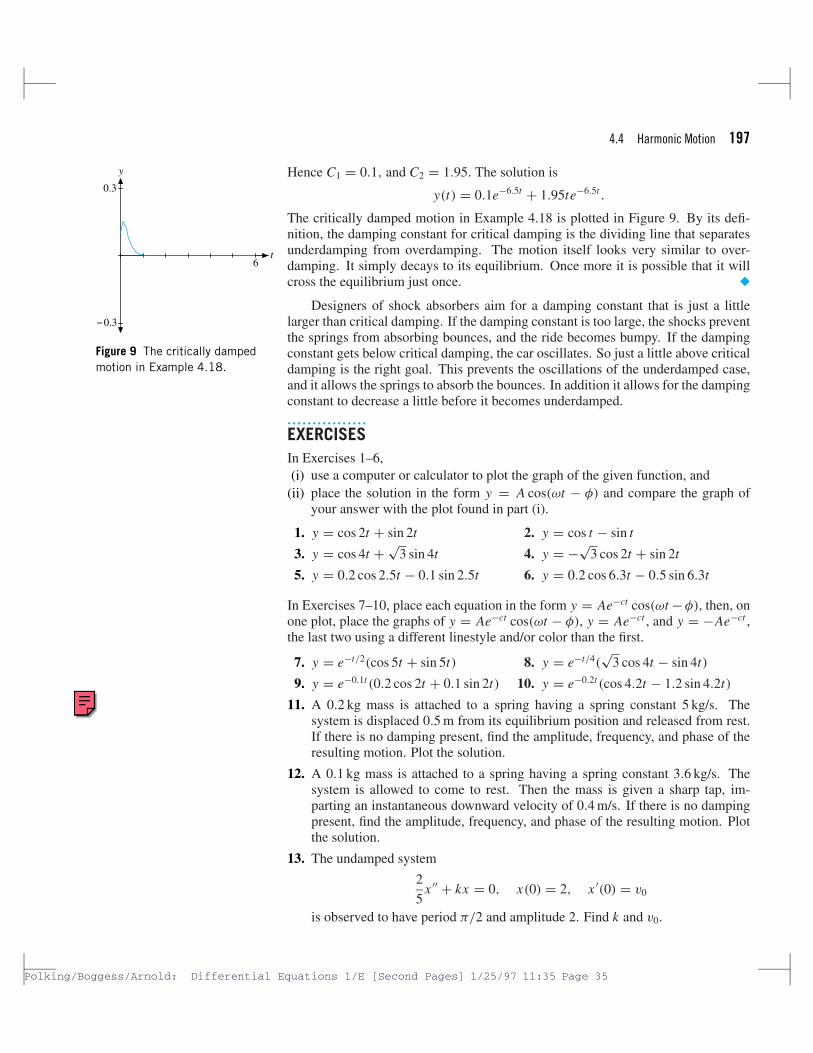
The critically damped motion in Example 4.18 is plotted in Figure 9. By its defi-nition, the damping constant for critical damping is the dividing line that separatesunderdamping from overdamping. The motion itself looks very similar to over-damping. It simply decays to its equilibrium. Once more it is possible that it willcross the equilibrium just once. �
Designers of shock absorbers aim for a damping constant that is just a littlelarger than critical damping. If the damping constant is too large, the shocks preventthe springs from absorbing bounces, and the ride becomes bumpy. If the dampingconstant gets below critical damping, the car oscillates. So just a little above criticaldamping is the right goal. This prevents the oscillations of the underdamped case,
t
y
6
−
0.3
0.3
Figure 9 The critically dampedmotion in Example 4.18.
and it allows the springs to absorb the bounces. In addition it allows for the dampingconstant to decrease a little before it becomes underdamped.................EXERCISESIn Exercises 1–6,(i) use a computer or calculator to plot the graph of the given function, and
(ii) place the solution in the form y = A cos(ωt − φ) and compare the graph ofyour answer with the plot found in part (i).
1. y = cos 2t + sin 2t 2. y = cos t − sin t
3. y = cos 4t + √3 sin 4t 4. y = −√
3 cos 2t + sin 2t
5. y = 0.2 cos 2.5t − 0.1 sin 2.5t 6. y = 0.2 cos 6.3t − 0.5 sin 6.3t
In Exercises 7–10, place each equation in the form y = Ae−ct cos(ωt −φ), then, onone plot, place the graphs of y = Ae−ct cos(ωt − φ), y = Ae−ct , and y = −Ae−ct ,the last two using a different linestyle and/or color than the first.
7. y = e−t/2(cos 5t + sin 5t) 8. y = e−t/4(√
3 cos 4t − sin 4t)
9. y = e−0.1t(0.2 cos 2t + 0.1 sin 2t) 10. y = e−0.2t(cos 4.2t − 1.2 sin 4.2t)
11. A 0.2 kg mass is attached to a spring having a spring constant 5 kg/s. Thesystem is displaced 0.5 m from its equilibrium position and released from rest.If there is no damping present, find the amplitude, frequency, and phase of theresulting motion. Plot the solution.
12. A 0.1 kg mass is attached to a spring having a spring constant 3.6 kg/s. Thesystem is allowed to come to rest. Then the mass is given a sharp tap, im-parting an instantaneous downward velocity of 0.4 m/s. If there is no dampingpresent, find the amplitude, frequency, and phase of the resulting motion. Plotthe solution.
13. The undamped system
2
5x ′′ + kx = 0, x(0) = 2, x ′(0) = v0
is observed to have period π/2 and amplitude 2. Find k and v0.
first lines of 11 and 12. spring constants are measured in kg/s2 (squared) 5 kg/s2 3.6 kg/s2 pex2
198 Chapter 4 Second-Order Equations
14. Consider the undamped oscillator
mx ′′ + kx = 0, x(0) = x0, x ′(0) = v0.
Show that the amplitude of the resulting motion is√
x20 + mv2
0/k.
15. A 2 µF capacitor (1 µF = 1 × 10⁻⁶ F) is charged to 20 V and then connectedacross a 6 µH inductor (1 µH = 1 × 10⁻⁶ H), forming an LC circuit.
(a) Find the initial charge on the capacitor.(b) At the time of connection, the initial current is zero. Assuming no resis-
tance, find the amplitude, frequency, and phase of the current. Plot thegraph of the current versus time. [Use equations (4.2) and (4.3) in Section3.4.]
16. A 1 kg mass, when attached to a large spring, stretches the spring a distance of4.9 m.
(a) Calculate the spring constant.(b) The system is placed in a viscous medium that supplies a damping constant
µ = 3 kg/s. The system is allowed to come to rest. Then the mass isdisplaced 1 m in the downward direction and given a sharp tap, impartingan instantaneous velocity of 1 m/s in the downward direction. Find theposition of the mass as a function of time and plot the solution.
17. Prove that an overdamped solution of my′′ + µy′ + ky = 0 can cross the timeaxis no more than once, regardless of the initial conditions. Use a numericalsolver to create a plot of an overdamped system that crosses the time axis onetime and a second plot where the plot does not cross the time axis.
18. A 50 g mass (1 kg = 1000 g) stretches a spring 20 cm (1 m = 100 cm). Finda damping constant µ so that the system is critically damped. If the mass isdisplaced 15 cm from its equilibrium position and released from rest, find theposition of the mass as a function of time and plot the solution.
19. Prove that a critically damped solution of my′′ + µy′ + ky = 0 can cross thetime axis no more than once, regardless of the initial conditions. Use a numer-ical solver to create a plot of an overdamped system that crosses the time axisone time and a second plot where the plot does not cross the time axis.
20. A spring mass system is modeled by the equation
x ′′ + µx ′ + 4x = 0.
(a) Show that the system is critically damped when µ = 4 kg/s.(b) Suppose that the mass is displaced upward 2 m and given an initial velocity
of 1 m/s. Use a numerical solver to plot the solution for c = 3.0, 3.5, 4.0,
. . . , 4.5, 5.0. Plot all solution curves on one figure. What is special aboutthe critically damped solution in comparison to the other solutions? Whywould you want to adjust the spring on a screen door so that it was criticallydamped?
21. If µ > 2√
km, the system mx ′′ + µx ′ + kx = 0 is overdamped. The system isallowed to come to equilibrium. Then the mass is given a sharp tap, impartingan instantaneous downward velocity v0.
remove dots in third line of 20(b). 4.5, 5.0. Plot pe
4.5 Inhomogeneous Equations; the Method of Undetermined Coefficients 199
(a) Show that the position of the mass is given by
x(t) = v0
γe−µt/(2m) sinh γ t, where γ =
√µ2 − 4mk
2m.
(b) Show that the mass reaches its lowest point at
t = 1
γtanh−1 2mγ
µ,
a time independent of the initial conditions.
(c) Show that, in the critically damped case, the time it takes the mass to reachits lowest point is given by t = 2m/µ.
22. A 100 g mass (1 kg = 1000 g) is hung from a spring having spring constant9.8 kg/s2. The system is placed in a viscous medium that imparts a force of0.3 N when the mass is moving at 0.2 m/s. Assume that the force applied bythe medium is proportional, but opposite, the mass’s velocity. The mass isdisplaced 10 cm from its equilibrium position and released from rest. Find theamplitude, frequency, and phase of the resulting motion. Plot the solution.
23. A capacitor (0.008 F) is charged to 50 V then connected in series with an induc-tor (4 H) and a resistor (20 �). Initially, there is no current in the circuit. Findthe amplitude, frequency, and phase of the current and plot its graph.
24. A 10 kg mass stretches a spring 1 m. The system is placed in a viscous mediumthat provides a damping constant µ = 20 kg/s. The system is allowed to attainequilibrium. Then a sharp tap to the mass imparts an instantaneous downwardvelocity of 1.2 m/s. Find the amplitude, frequency, and phase of the resultingmotion. Plot the solution.
25. A capacitor (0.02 F) is charged to 1 V then connected in series with an inductor(10 H) and a resistor (40 �). Initially, there is no current in the circuit. Find theamplitude, frequency, and phase of the current and plot its graph.
4.5 Inhomogeneous Equations; the Method of Undetermined CoefficientsWe now turn to the solution of inhomogeneous linear equations. These are equationsof the form
y′′ + py′ + qy = f, (5.1)
where p = p(t), q = q(t), and f = f (t) are functions of the independent variable.Remember that f is called the inhomogeneous term, or the forcing term.
Our solution strategy comes from the understanding of the structure of the gen-eral solution, which is contained in the next theorem.
THEOREM 5.2 Suppose that yp is a particular solution to the inhomogeneous equation (5.1), andthat y1 and y2 form a fundamental set of solutions to the associated homogeneousequation
Change the last sentence in Exercise 25 to: Find the amplitude, frequency, and phase of the charge on the capacitor and plot its graph.
200 Chapter 4 Second-Order Equations
Then the general solution to the inhomogeneous equation (5.1) is given by
y = yp + C1 y1 + C2 y2
where C1 and C2 are arbitrary constants.
Notice that the general solution can be written as y = yp + yh , where yh =C1 y1 + C2 y2 is the general solution to the corresponding homogeneous equation.Thus, to find the general solution to the inhomogeneous equation (5.1) we first findthe general solution, yh , to the corresponding homogeneous equation (5.3). Next,we find a particular solution, yp, to the inhomogeneous equation. The general solu-tion to the inhomogeneous equation is then y = yp + yh .
Proof Suppose that y is a solution to (5.1). We are given that yp is also a solution,so we have the two equations
y′′ + py′ + qy = f, and
y′′p + py′
p + qyp = f,
Subtracting we get
(y − yp)′′ + p(y − yp)
′ + q(y − yp) = 0.
Therefore, y − yp is a solution to the associated homogeneous equation (5.3). Sincey1 and y2 form a fundamental set of solutions, there are constants C1 and C2 suchthat
y − yp = C1 y1 + C2 y2.
Consequently,y = yp + C1 y1 + C2 y2
as promised.
For equations with constant coefficients, we already know how to solve the ho-mogeneous equation, so in this section we will concentrate on finding one particularsolution to the inhomogeneous equation.
The method of undetermined coefficientsWe will be looking at the inhomogeneous equation
y′′ + py′ + qy = f, (5.4)
where p and q are constants and f = f (t) is a function of the independent variable.The method of undetermined coefficients only works if the coefficients are con-stants. Second-order equations are the most important applications of the method,but the method works for higher-order equations in exactly the same way that it doesfor second-order equations. For simplicity and convenience we will emphasize thesecond-order case.
The method of undetermined coefficients is based on the fact that there are somesituations where the form of the forcing term in (5.4) allows us to almost guess theform of a particular solution. Let’s highlight the key idea.
4.5 Inhomogeneous Equations; the Method of Undetermined Coefficients 201
If the forcing term f has a form that is replicated under differen-tiation, then look for a solution with the same general form as theforcing term.
Exponential forcing termsThe easiest example of such a forcing term is an exponential function f (t) = eat .Then f ′(t) = aeat , which is also an exponential function. The method is illustratedby our first example.
E X A M P L E 5 . 5 � Find a particular solution to the equation
y′′ − y′ − 2y = 2e−2t . (5.6)
The forcing term is f (t) = 2e−2t . We look for a particular solution with thesame form as f , or
y(t) = ae−2t ,
where a is an as yet undetermined coefficient. Its derivatives are
y′(t) = −2ae−2t and y′′(t) = 4ae−2t .
If we insert these expressions into the left-hand side of (5.6), we get
As we will see, we will need both the cosine and the sine terms, even though only asine term appears in the forcing term.
The derivatives of y are
y′ = −3a sin 3t + 3b cos 3t and
y′′ = −9a cos 3t − 9b sin 3t.
Insert these expressions into the left-hand side of (5.8).
y′′ + 2y′ − 3y = (−9a cos 3t − 9b sin 3t) + 2(−3a sin 3t + 3b cos 3t)
− 3(a cos 3t + b sin 3t)
= (−12a + 6b) cos 3t + (−6a − 12b) sin 3t.
(5.9)
Equating the coefficients of the sine and cosine terms in (5.8) and (5.9) gives twoequations for a and b,
−12a + 6b = 0
−6a − 12b = 5,
with solutions a = −1/6 and b = −1/3. Hence, a particular solution is
y = −1
6cos 3t − 1
3sin 3t. (5.10)
�
The complex methodThere is another way to find a particular solution in situations where the forcingfunction contains a trigonometric term. We will illustrate the method by solving thesame equation as we did in Example 5.7.
E X A M P L E 5 . 1 1 � Use the complex method to find a particular solution to the equation
y′′ + 2y′ − 3y = 5 sin 3t. (5.12)
Notice that the right-hand side of (5.12) is 5 sin 3t = Im(5e3i t). Instead ofsolving (5.12) directly as we did in Example 5.7, we will look for a solution to
z′′ + 2z′ − 3z = 5e3i t (5.13)
using the techniques of Example 5.5. If z(t) = x(t) + iy(t) is that solution, thenformally we have
4.5 Inhomogeneous Equations; the Method of Undetermined Coefficients 203
On the other hand, expanding the right-hand side of (5.13) using Euler’s formula,we get
z′′ + 2z′ − 3z = 5e3i t = 5[cos 3t + i sin 3t]. (5.15)
Equating the imaginary parts of (5.14) and (5.15), we see that y(t) = Im z(t) isa solution to (5.12). We notice in passing that x(t) = Re z(t) is a solution to theequation
x ′′ + 2x ′ − 3x = 5 cos 3t.
Our solution to (5.13) should have the same form as the forcing term, so we tryz(t) = ae3i t . Substituting this into the left-hand side of (5.13), we get
z′′ + 2z′ − 3z = (3i)2ae3i t + 2(3i)ae3i t − 3ae3i t = −6(2 − i)ae(3i)t .
For z to be a solution of (5.13) we must have −6(2 − i)a = 5. Therefore,
a = −1
6
5
2 − i= −1
6
5
2 − i
2 + i
2 + i= −1
6
10 + 5i
5= −2 + i
6.
Hence the complex solution is
z(t) = −2 + i
6e3i t
= −1
6(2 + i)(cos 3t + i sin 3t)
= −1
6{[2 cos 3t − sin 3t] + i[cos 3t + 2 sin 3t]} .
The solution y to (5.12) is the imaginary part of z, or
y(t) = −1
6[cos 3t + 2 sin 3t],
which agrees with (5.10). �
It is up to the individual to decide which of these methods is preferable. Ifyou are comfortable with complex arithmetic, then the complex method is probablyquicker. The complex method is preferred by some engineers and physicists becauseof the insight the answers provide.
Polynomial forcing termsThe derivative of a polynomial is another polynomial of lower degree. Conse-quently, a polynomial forcing term
f (t) = a0tn + a1tn−1 + · · · + an−1t + an
has a form which is replicated under differentiation. We can find a particular solu-tion by the method of undetermined coefficients.
E X A M P L E 5 . 1 6 � Find a particular solution to the differential equation
y′′ + 2y′ − 3y = 3t + 4. (5.17)
The right-hand side is a polynomial of degree 1, so we look for a particularsolution of the same form. In this case that means a polynomial of the same degree,or
y = at + b,
where a and b are constants to be determined. The derivatives of y are
y′ = a and y′′ = 0.
Inserting these into our differential equation gives
Equating the coefficient of t and the constant term in (5.17) and (5.18) gives twoequations for a and b
−3a = 3,
2a − 3b = 4.
The solutions are a = −1 and b = −2, and our particular solution is
y = −t − 2.
We encourage the reader to check that y is indeed a solution. �
Exceptional casesThe method of undetermined coefficients looks straightforward. There are, however,some exceptional cases to look out for. Suppose we change the forcing term inequation (5.6) in Example 5.5 to 3e−t , getting the equation
y′′ − y′ − 2y = 3e−t .
If we look for a solution of the indicated form, y(t) = ae−t , we run into trouble. Tosee this, let’s insert y into the left-hand side of the differential equation. We get
y′′ − y′ − 2y = ae−t + ae−t − 2ae−t = 0.
There is no choice of the constant a which will make this equal to 3e−t .The problem arises because the forcing term, and hence the proposed solution,
is a solution to the associated homogeneous equation. This is the source of thedifficulty in all exceptional cases. However, even if the solution to the homogeneousequation is only a part of the forcing term, we can have an exceptional case. As wewill see, exceptional cases do arise in applications, and they are often the mostinteresting cases.
What do we do? In this case we look for a solution of the form y(t) = ate−t .We multiply the usual general form by t . This is the way to find a solution wheneverthe usual form does not work. If this method does not work, multiply by t once moreand try again.
4.5 Inhomogeneous Equations; the Method of Undetermined Coefficients 205
E X A M P L E 5 . 1 9 � Find a particular solution to the equation
y′′ − y′ − 2y = 3e−t . (5.20)
We know from the preceding discussion that the forcing term is a solution tothe homogeneous equation, so we look for a solution of the form y(t) = ate−t .Substituting into the left-hand side of the equation, we get
Therefore, we need a = −1, and our particular solution is y(t) = −te−t . �
Typically, we do not notice that the forcing function is exceptional. The firstindication that arises is when we are presented with equations for the undeterminedcoefficients that are inconsistent. At this point apply the remedy—multiply the trialsolution by t and try again. If that still leads to inconsistent equations, multiplyby t2.
Combination forcing termsThe method we just used can be used whenever the forcing term is a linear combi-nation of expressions of the forms we have already handled.
E X A M P L E 5 . 2 1 � Find a particular solution to the equation
y′′ − y′ − 2y = e−2t − 3e−t . (5.22)
The forcing term is a sum, f (t) = f1(t) + f2(t), where f1(t) = e−2t , andf2(t) = −3e−t . Suppose we break up the equation and solve the equations sepa-rately for each part of the forcing term. This means that we find functions y1 and y2
such that
y′′1 − y′
1 − 2y1 = e−2t , and
y′′2 − y′
2 − 2y2 = −3e−t .(5.23)
Adding these two equations, we get
(y1 + y2)′′ − (y1 + y2)
′ − 2(y1 + y2) = e−2t − 3e−t ,
so y = y1 + y2 is a solution to (5.22).It remains to solve the two equations in (5.23). The first is solved using the
method in Example 5.5. We find that y1(t) = e−2t/4. In the second equation wehave an exceptional case, so we use the method of Example 5.19. The solution isy2(t) = te−t . Hence the solution to (5.22) is
As the example illustrates, when the forcing term is a linear combination of theterms, we need only solve the equation for each individual term and take the linearcombination of the solutions.
Let’s look at one more example.
E X A M P L E 5 . 2 4 � Find a particular solution to the equation
y′′ + 4y = cos 2t − 2 sin 2t. (5.25)
We will use the complex method. It is easiest to treat the two summands inthe forcing term separately. This means that we look for solutions y1 and y2 to theequations
y′′1 + 4y1 = cos 2t and
y′′2 + 4y2 = −2 sin 2t.
(5.26)
Then it is easily seen that y = y1 + y2 is a solution to (5.25).To solve the first equation in (5.26), we notice that cos 2t = Re(e2i t), so we
solve the complex equation
z′′ + 4z = e2i t . (5.27)
The forcing term is a solution to the homogeneous equation, so we look for a solu-tion of the form z(t) = ate2i t . In the usual way we find that the solution is
z(t) = − i t
4e2i t .
The solution to the first equation in (5.26) is
y1(t) = Re z(t) = Re
(− i t
4e2i t
)= t sin 2t
4.
Notice that the imaginary part of z,
u(t) = Im z(t) = Im
(− i t
4e2i t
)= − t cos 2t
4,
is a solution to the equation
u′′ + 4u = Im e2i t = sin 2t.
The similarity between this equation and the second equation in (5.26) allows us toconclude that
4.5 Inhomogeneous Equations; the Method of Undetermined Coefficients 207
More complicated forcing termsIn addition to the three cases we have considered so far, we could have forcing termswhich are products of two of these, or of all three. The most general situation wouldbe a forcing term of the form
f (t) = ert P(t) cos ωt + ert Q(t) sin ωt,
where P(t) and Q(t) are polynomials. Again f ′(t) has the same form, so we canuse undetermined coefficients.
The method of undetermined coefficients is summarized in Table 1, whichshows the allowed forcing functions and the type of particular solution to be used.Even for the most general case the method works in the way we have indicated inour examples.
Table 1 The method of undetermined coefficients
Forcing function f (t) Trial solution yp(t) Comments
ert aert
cos ωt or sin ωt a cos ωt + b sin ωt
P(t) p(t) P is a polynomial;p is a polynomial
of the same degree
P(t) cos ωt or p(t) cos ωt+ P is a polynomial;P(t) sin ωt q(t) sin ωt p & q are polynomials
of the same degree
ert cos ωt or ert [a cos ωt+ert sin ωt b sin ωt]
ert P(t) cos ωt or ert [p(t) cos ωt+ P is a polynomial;ert P(t) sin ωt q(t) sin ωt] p & q are polynomials
of the same degree
................EXERCISES
In Exercises1–4, use the technique demonstrated in Example 5.5 to find a particularsolution for the given differential equation.
In Exercises 18–23, use the technique of Section 4.3 to find a solution of the as-sociated homogeneous equation, then use the technique of this section to find aparticular solution. Use Theorem 5.2 to form the general solution. Then find thesolution satisfying the given initial conditions.
21. y′′ − 2y′ + 5y = 3 cos t , y(0) = 0, y′(0) = −2
22. y′′ + 4y′ + 4y = 4 − t , y(0) = −1, y′(0) = 0
23. y′′ − 2y′ + y = t3, y(0) = 1, y′(0) = 0
In Exercises 24–29, the forcing term is also a solution of the associated homoge-neous solution. Use the technique of Example 5.19 to find a particular solution.
show that z(t) = αy f (t) + βyg(t) is a solution of
y′′ + py′ + qy = α f (t) + βg(t),
where α and β are any real numbers.
Use the technique suggested by Examples 5.21 and 5.24, as well as Exercise 30, tohelp find particular solutions for the differential equations in Exercises 31–38.
31. y′′ + 2y′ + 2y = 2 + cos 2t 32. y′′ − y = t − e−t
44. Use the form yp = e−2t(a cos t + b sin t) in an attempt to find a particularsolution of y′′ + 2y′ + 2y = e−2t sin t .
45. If z(t) = x(t) + iy(t) is a solution of
z′′ + pz′ + qz = Ae(a+bi)t ,
show that x(t) and y(t) are solutions of
x ′′ + px ′ + qx = Aeat cos bt and y′′ + py′ + qy = Aeat sin bt,
respectively.
46. Use the technique suggested by Exercise 45 to find a particular solution of theequation in Exercise 44.
47. Prove that the imaginary part of the solution of z′′ + z′ + z = teit is a solution ofy′′ + y′ + y = t sin t . Use this idea to find a particular solution of y′′ + y′ + y =t sin t .
4.6 Variation of ParametersIn this section we introduce a technique called variation of parameters. This tech-nique is used to find a particular solution to more general higher-order equations,provided we know a fundamental set of solutions to the associated homogeneousequation. As we did in the previous section, we will illustrate the method for second-order equations. The method also works for higher-order equations, but it is usuallymore efficient to solve the associated first-order system using variation of parame-ters. This will be discussed in a later chapter.
Notice that we are allowing the coefficients p(t) and q(t) to be functions of t . Inparticular, we are not restricting them to be constants. This might seem to be a greatincrease in generality, but there is a rather strong constraint. We will have to assumethat we have computed a fundamental set of solutions y1 and y2 to the associatedhomogeneous equation
y′′ + p(t)y′ + q(t)y = 0. (6.2)
Then the general solution to the homogeneous equation is
yh = C1 y1 + C2 y2, (6.3)
where C1 and C2 are arbitrary constants.The idea behind variation of parameters is to replace the constants C1 and C2
in (6.3) by unknown functions v1(t) and v2(t) and look for a particular solution tothe inhomogeneous equation (6.1) of the form
yp = v1 y1 + v2 y2. (6.4)
You will notice the similarity with the method of variation of parameters as it wasused to solve first-order linear equations in Chapter 2.
E X A M P L E 6 . 5 � Find a particular solution to the equation
y′′ + y = tan t. (6.6)
The right side, tan t , is not one of the forms that can be handled with undeter-mined coefficients. We will find a solution by the method of variation of parameters.First, note that y1(t) = cos t and y2(t) = sin t are a fundamental set of solutionsto the associated homogeneous equation y′′ + y = 0. So we look for a particularsolution of the form
yp = v1 cos t + v2 sin t. (6.7)
We start by computing the first derivative of yp.
y′p = v′
1 cos t − v1 sin t + v′2 sin t + v2 cos t
= (v′1 cos t + v′
2 sin t) − v1 sin t + v2 cos t(6.8)
The differential equation (6.6) puts only one constraint on the two functions v1
and v2. We can impose one more constraint. Notice that if we set the term inparentheses on the right in (6.8) equal to zero, then the expression simplifies, andwe will eliminate the first derivatives of v1 and v2. Then when we compute y′′
p nosecond derivatives of v1 and v2 will appear. Hence we set
Inserting these expressions for yp and y′′p into the left-hand side of our differential
equation, we obtain
y′′p + yp = (−v′
1 sin t + v′2 cos t − v1 cos t − v2 sin t
) + (v1 cos t + v2 sin t)
= −v′1 sin t + v′
2 cos t.
Comparing this with (6.6), we see that yp is a solution to (6.6) provided −v′1 sin t +
v′2 cos t = tan t. This is our second equation for v′
1 and v′2. Let’s restate it along
with (6.9).
v′1 cos t + v′
2 sin t = 0
−v′1 sin t + v′
2 cos t = tan t
This is a system of two linear equations for the unknowns v′1 and v′
2. Thecoefficient matrix is (
cos t sin t− sin t cos t
).
The system can be solved provided the determinant of this matrix is nonzero. Sincethe determinant is cos2 t +sin2 t = 1, we can solve. Let’s solve them by elimination.Multiply the first by sin t and the second by cos t to get
sin t (v′1 cos t + v′
2 sin t) = 0
cos t (−v′1 sin t + v′
2 cos t) = sin t.
When added together, the term involving v′1 is eliminated:
v′2(sin2 t + cos2 t) = sin t or v′
2 = sin t.
Similarly, if we multiply the first equation by cos t and the second by sin t and thensubtract the second from the first, we get
v′1(cos2 t + sin2 t) = v′
1 = − sin t tan t or v′1 = −sin2 t
cos t.
When we integrate the equations for v′1 and v′
2, we get
v1(t) = − ln | sec t + tan t | + sin t and v2(t) = − cos t. (6.10)
Notice that we have left off the constants of integration. Since we are after oneparticular solution, we can set the constants equal to zero.
Substituting the formulas for v1 and v2 into 6.7 gives our particular solution
yp(t) = (− ln | sec t + tan t | + sin t) cos t − cos t sin t
This is a system of two linear equations for v′1 and v′
2. The coefficient matrix is(y1 y2
y′1 y′
2
).
The system can be solved provided that the determinant of this matrix is nonzero.The determinant will be recognized as the Wronskian of y1 and y2,
W = y1 y′2 − y2 y′
1.
Since y1 and y2 form a fundamental set of solutions to the homogeneous equation,they are linearly independent and we know by Proposition 1.26 that the WronskianW (t) �= 0.
These equations can be solved by elimination (multiply the first by y′1 and the
second by y1 and then subtract) to obtain
v′2 = y1g
y1 y′2 − y′
1 y2and v′
1 = −y2g
y1 y′2 − y′
1 y2.
Notice that the denominator in the above expressions is the Wronskian of y1 and y2
and is always nonzero.We can integrate these equations:
v1(t) =∫ −y2(t)g(t) dt
y1(t)y′2(t) − y′
1(t)y2(t), and
v2(t) =∫
y1(t)g(t) dt
y1(t)y′2(t) − y′
1(t)y2(t).
(6.16)
When they are inserted into (6.12), we get a particular solution.
SummaryTo find a particular solution to the inhomogeneous equation y′′ + py′ + qy = g,follow these steps.
1. Find a fundamental set of solutions y1, y2 to the associated homogeneous equa-tion y′′ + py′ + qy = 0.
2. Form yp = v1 y1 + v2 y2 where v1 and v2 are functions to be determined.
3. Find v1 and v2. Here there are two possible ways to proceed. The first way is touse the formulas in (6.16). This requires that you remember these formulas orthat you have the use of a book that contains the formulas.
The second way is to follow the procedure of the method of variation of param-eters. The procedure has the following steps:(a) Differentiate yp:
y′p = (v′
1 y1 + v′2 y2) + v1 y′
1 + v2 y′2
and set the first term on the right equal to zero.
(b) Take the second derivative of yp and insert yp, y′p, and y′′
p into the differen-tial equation. After simplifying, a second equation will appear:
v′1 y′
1 + v′2 y′
2 = g(t). (6.18)
(c) Solve (6.17) and (6.18) for v′1 and v′
2 by elimination.
(d) Integrate to find v1 and v2.
4. Substitute v1 and v2 into yp = v1 y1 + v2 y2.
It is up to the reader to decide which of the methods to use in step 3.Although variation of parameters always works theoretically, its success re-
quires a fundamental set of solutions to the homogeneous equation and the abilityto compute the integrals in (6.16). The method is of significant theoretical impor-tance, however.
................EXERCISES
For Exercises 1–12, find a particular solution to the given second-order differentialequation.
1. y′′ + 9y = tan(3t) 2. y′′ + 4y = sec(2t)
3. y′′ − y = t + 3 4. x ′′ − 2x ′ − 3x = 4e3t
5. y′′ − 2y′ + y = et 6. x ′′ − 4x ′ + 4x = e2t
7. x ′′ + x = tan2 t 8. x ′′ + x = sec2 t
9. x ′′ + x = tan3 t 10. x ′′ + x = sec3 t
11. y′′ + y = tan t + sin t + 1 12. y′′ + y = sec t + cos t − 1
13. Verify that y1(t) = t and y2(t) = t−3 are solutions to the homogeneous equa-tion
t2 y′′(t) + 3t y′(t) − 3y(t) = 0.
Use variation of parameters to find the general solution to
t2 y′′(t) + 3t y′(t) − 3y(t) = 1
t.
14. Verify that y1(t) = t−1 and y2(t) = t−1 ln t are solutions to the homogeneousequation
t2 y′′(t) + 3t y′(t) + y(t) = 0, for t > 0.
Use variation of parameters to find the general solution to
4.7 Forced Harmonic MotionIn this section, we apply the technique of undetermined coefficients to analyze har-monic motion with an external sinusoidal forcing term. We derived the model inSection 4.4, and with a sinusoidal forcing term, equation (4.4) becomes
x ′′ + 2cx ′ + ω20x = A cos ωt. (7.1)
The constant A is the amplitude of the driving force, and ω is the driving frequency.To focus our thinking, we may suppose that we have an iron mass m suspended
on a spring, with the top of the spring attached to a motor that moves the top ofthe spring up and down. We can also consider an RLC circuit in which the sourcevoltage is sinusoidal.
We will first treat the case with no damping.
Forced undamped harmonic motionThe equation we will deal with here comes from (7.1) with c = 0 or
x ′′ + ω20x = A cos ωt. (7.2)
The associated homogeneous equation is
x ′′ + ω20x = 0, (7.3)
with general solutionxh = C1 cos ω0t + C2 sin ω0t.
We have to consider separately the cases when the driving frequency ω is equalto the natural frequency and when it is not.
Case 1: ω �= ω0. If the driving frequency is not equal to the natural frequency, welook for a particular solution of the form
x p = a cos ωt + b sin ωt, (7.4)
where a and b are undetermined constants. Substituting x p into the left-hand sideof the inhomogeneous differential equation (7.2) gives
x ′′p + ω2
0x p = a(ω20 − ω2) cos ωt + b(ω2
0 − ω2) sin ωt.
Comparing this with (7.2), we see that we have a solution provided that
Notice that x p is oscillatory, with the same frequency as the driving force. Theamplitude of this oscillation also depends on the driving frequency and gets largeras the driving frequency approaches the natural frequency of the spring. This is ourfirst indication of resonance. We will have more to say about that shortly.
The general solution to the inhomogeneous equation is
x(t) = xh(t) + x p(t) = C1 cos ω0t + C2 sin ω0t + A
ω20 − ω2
cos ωt.
Let’s look at the solution where the motion starts at equilibrium. This means theinitial conditions are x(0) = x ′(0) = 0. It is easily seen that C1 = −A/(ω2
0 − ω2),
and C2 = 0. Hence the solution is
x(t) = A
ω20 − ω2
(cos ωt − cos ω0t). (7.5)
This is a superposition of two oscillations with different frequencies. The result isinteresting.
E X A M P L E 7 . 6 � Suppose A = 23, ω0 = 11, and ω = 12. With these values of the parameters thesolution (7.5) becomes
x(t) = cos 11t − cos 12t.
The graph is shown in Figure 1. This figure shows the phenomenon called beats. Itoccurs whenever two frequencies that are almost equal interfere with each other aswe see in (7.5). �
−6 −4 −2 0 2 4 6
−2
−1.5
−1
−0.5
0
0.5
1
1.5
2
t
x
Figure 1 Beats in forced, undamped, harmonic motion.
We can understand the phenomenon of beats better after a little algebra. Weintroduce ω = (ω0 + ω)/2, which is the mean frequency, and δ = (ω0 − ω)/2, thehalf difference. Then
ω = ω − δ and ω0 = ω + δ.
The relationship between these variables is shown in Figure 2. If we substitute theseequations into (7.5) and use the addition law for the cosine, we get
x(t) = A sin δt
2ωδsin ωt. (7.7)
In Example 7.6, δ = −1/2 and ω = 23/2. In that case the factor sin δt =sin(−t/2) oscillates very slowly, especially in comparison with the faster oscillation
ω ω ω0
δ δ
Figure 2 The relationship of ω
and ω0 to ω and δ.
with frequency ω = 23/2. Thus the solution in (7.7) can be seen to be a fastoscillation with a frequency ω and an amplitude∣∣∣∣ A sin δt
2ωδ
∣∣∣∣ , (7.8)
which oscillates much more slowly. If we were to superimpose a graph of this slowoscillating amplitude on the graph in Figure 1, it would appear as a curve through themaxima of the faster oscillation. This is called the envelope of the faster oscillation.(See Exercise 2.)
The phenomenon of beats illustrated in Figure 1 occurs in many situations. Forexample, it is used by a piano tuner to be sure that particular piano strings are prop-erly tuned. The tuner strikes a tuning fork, which vibrates at the correct frequency.He next hits the poorly tuned piano key, which vibrates at a slightly different fre-quency. The two sounds interfere in a way modeled by (7.5), and therefore by (7.7).The tuner hears the mean frequency with an amplitude that is modulated by the dif-ference frequency, as shown in Figure 1. This modulation gives rise to beats in thetone that are readily audible. When the string is properly tuned, the beats go away.
Case 2: ω = ω0. In this case, the particular solution given in (7.4) is a solution tothe homogeneous equation. Therefore, we look for a particular solution of the form
x p = t (a cos ω0t + b sin ω0t).
Inserting x p into the left-hand side of the differential equation in 7.2, we get
x ′′p + ω2
0x p = [2ω0(−a sin ω0t + b cos ω0t) + tω2
0(−a cos ω0t − b sin ω0t)]
+ ω20t (a cos ω0t + b sin ω0t)
= 2ω0(−a sin ω0t + b cos ω0t).
Setting the right side equal to A cos ω0t , we see that we have a solution providedthat
and the general solution to the inhomogeneous equation is
x(t) = xh(t) + x p(t) = C1 cos ω0t + C2 sin ω0t + A
2ω0t sin ω0t.
In the special case where x(0) = C1 = 0, x ′(0) = C2 = 0, A = 8, and ω0 = 4,this reduces to
x(t) = t sin 4t.
The graph of this function is shown in Figure 3. Notice how the solution growswith time. This growth is due to the fact that the frequency of the forcing termequals the natural vibrating frequency of the spring. The force pulls and pushesat a frequency equal to the natural frequency of the spring. Thus the amplitudeof the oscillatory motion of the mass increases. This type of behavior is calledresonance, and engineers try to eliminate it in the design of mechanical systems,since oscillations that grow in amplitude can eventually cause the system to break.
0 2 4 6 8 10 12
−15
−10
−5
0
5
10
15
t
x
Figure 3 Forced, undamped, harmonic motion where thedriving frequency equals the natural frequency.
In reality, mechanical systems always have some damping (friction) that willkeep the solution from getting infinitely large. However, resonance can still causemechanical motions to become large enough to cause major structural damage. Acommon example of the destructiveness of resonance is the shattering of a glass bythe voice of a singer. The singer has to sing a note at a frequency that is very closeto the natural frequency of the glass in order to cause it to resonate and eventuallyshatter. Another example involves the behavior of a troop of soldiers marching overa bridge. If they were to continue to march in perfect step, they might be marchingat the natural frequency of some component of the bridge and cause it to resonateand eventually break. Consequently, since time immemorial troops of soldiers havebroken ranks when marching over a bridge.
On the other hand, resonance is exploited in electrical systems that are governedby the same model as (7.2) in order to tune radios, for example.
Forced damped harmonic motionIf we add a damping term to the system, interesting things happen. Now we aredealing with the equation in (7.1),
x ′′ + 2cx ′ + ω20x = A cos ωt. (7.9)
The associated homogeneous equation is
x ′′ + 2cx ′ + ω20x = 0. (7.10)
The characteristic roots are
λ = −c ±√
c2 − ω20.
Let’s suppose that we are in the underdamped case, where c < ω0. We found inSection 4.4 that the general solution is
xh = e−ct (C1 cos(ηt) + C2 sin(ηt)) ,
where
η =√
ω20 − c2.
To find a particular solution to the inhomogeneous equation, we use undeter-mined coefficients, but this time it is easier to use the complex method. This meanswe look for a solution z(t) = aeiωt to the equation
z′′ + 2cz′ + ω20z = Aeiωt (7.11)
and then set x p = Re(z). Let’s substitute z(t) into the left side of (7.11). We get
z′′ + 2cz′ + ω20z = [
(iω)2 + 2c(iω) + ω20
]aeiωt = P(iω)z,
where the polynomialP(λ) = λ2 + 2cλ + ω2
0
is the characteristic polynomial of the differential equation in (7.11) or (7.10). Thusequation (7.11) becomes
P(iω)z(t) = Aeiωt .
The solution is
z(t) = 1
P(iω)Aeiωt = H(iω)Aeiωt , (7.12)
where we have set
H(iω) = 1
P(iω).
The function H(iω) is called the transfer function. To see what it is like, welook at its reciprocal
We want to write this complex number in polar form, which means that we want tofind a positive number R and an angle φ such that
P(iω) = Reiφ = R[cos φ + i sin φ].We need
R cos φ = ω20 − ω2 and R sin φ = 2cω.
This is just polar coordinates, so
R =√
(ω20 − ω2)2 + 4c2ω2,
while the angle φ is defined by the pair of equations
cos φ = ω20 − ω2√
(ω20 − ω2)2 + 4c2ω2
and sin φ = 2cω√(ω2
0 − ω2)2 + 4c2ω2.
(See the discussion of amplitude and phase in Section 4.4.) Notice that 2cω > 0, sosin φ > 0. This means that the phase always satisfies 0 < φ < π . Furthermore, wehave
cot φ = ω20 − ω2
2cωor φ = φ(ω) = arccot
(ω2
0 − ω2
2cω
). (7.13)
The last equation defines φ uniquely because 0 < φ < π .Now we see that the transfer function can be written as
H(iω) = 1
P(iω)= 1
Re−iφ.
We will define the gain G by
G(ω) = 1
R= 1√
(ω20 − ω2)2 + 4c2ω2
, (7.14)
and then the transfer function is
H(iω) = G(ω)e−iφ(ω). (7.15)
From (7.12) we see that the solution to (7.11) is
z(t) = H(iω)Aeiωt = G(ω)Aei(ωt−φ).
Finally, the solution to (7.9) is
x p(t) = Re z(t) = G(ω)A cos(ωt − φ). (7.16)
This form makes it clear that x p is sinusoidal with the same frequency as the drivingforce. It also shows that the amplitude of x p is the product of the gain G(ω) timesthe amplitude of the driving force. In addition, x p is out of phase with the drivingforce by the amount φ = φ(ω), given in (7.13).
Notice that xh has the factor e−ct , which quickly decays to 0 as t → ∞. For thisreason, this term is called the transient term. The rate of the decay of the transientterm is governed by the exponential factor e−ct . After the passage of time equal toTc = 1/c, this decreases to e−1 ≈ 0.3679, and the amplitude of the transient termhas decreased to e−1 times its original value. Tc is called the time constant, and itis defined by this property. Notice that after the passage of time equal to 4Tc theamplitude of the transient is reduced to e−4 ≈ 0.0183 times its original value, afterwhich the effect of the transient term is usually negligible.
The particular solution x p in (7.16) does not decay. It is therefore called thesteady-state term. It is this term that is driven by the external force A cos ωt . Afterthe passage of time equal to a few time constants, it is the only term that is important.
E X A M P L E 7 . 1 8 � Consider a forced vibrating spring where m = 5kg, µ = 7 kg/s, and k = 3 kg/s2,with a forcing term 2 cos 4t . Suppose the initial conditions are such that the con-stants in (7.17) are C1 = 0 and C2 = 1. Find the amplitude and the phase of thesteady-state solution. Plot the displacement of the resulting oscillation versus time.Add a plot of the steady-state oscillation.
The equation for the vibrating spring with the given parameters is
5x ′′ + 7x ′ + 3x = 2 cos 4t.
Dividing by the mass 5, we get
x ′′ + 7
5x ′ + 3
5x = 2
5cos 4t.
This is the form of the equation for the forced harmonic oscillator. The naturalfrequency is ω0 = √
3/5 ≈ 0.7746. In addition, c = 7/10. With the assumptions ofthe example, the transient solution is
xh(t) = e−ct sin ηt,
where η =√
ω20 − c2 ≈ 0.3317. The gain is computed from (7.14) to be G(4) ≈
0.0610. Hence the amplitude of the steady-state solution is G(4)× (2/5) ≈ 0.0244.
Finally, we compute the phase from (7.13) and get φ = φ(4) = 2.7928. A plot ofthe solution together with its steady-state term is given in Figure 4. Note how thesolution x converges to the steady-state solution as t gets large. �
Transient solutions can be quite large in comparison to the steady-state solution,as we have seen in Example 7.18, as shown in Figure 4. Such large transient currentsin electrical circuits can be destructive. It is almost certain that you have experiencedthis. Transients arise whenever an electrical circuit is turned on or off. How oftenhave you turned on a light and one of the bulbs burned out immediately? This iscaused by a large transient current flowing through an already weakened bulb. How
Figure 4 The motion of a forced spring. The steady-statesolution is in blue.
often have you turned on a light and one of the bulbs was burned out, although ithad been working fine the last time you used the light? This time the bulb mostlikely burned out when the lights were turned out, and again it was a large transientcaused by the shutdown that did the job.
The destructive effect of transients is the reason why it is often a good idea toleave electrical equipment running even when it is not being used. For example, it ishighly recommended that computers be always left on, unless it is known that theywill not be used for a couple of days at the minimum. Transients are particularlyharmful to hard disks.
We now examine the steady-state term (7.16) more closely. We will concentrateon the amplitude. We will examine how the gain G depends on the driving frequencyω. There are too many terms in the formula (7.14) for G to easily understand whatwill happen for all possible values of the parameters. We remedy this by lumpingparameters. First, we will want to see how G changes as the driving frequencychanges relative to the natural frequency, so we will introduce s = ω/ω0 by settingω = sω0 and consider G as a function of s. Then we introduce D = 2c/ω0, bysubstituting c = Dω0/2. The new constant D measures the effect of the dampingforce. When these changes are introduced, the gain takes the simpler form
G = 1
ω20
√(1 − s2)2 + D2s2
, where s = ω
ω0and D = 2c
ω0.
While still somewhat complicated, this expression for the gain is much easier tounderstand than (7.14). It allows us to easily see how the gain varies as the quotients = ω/ω0 varies. Because the natural frequency is fixed, let’s look at the quantity
ω20G = 1√
(1 − s2)2 + D2s2.
The behavior of ω20G as a function of s and D is shown in Figure 5. If the natural
frequency ω0 is also fixed, then D = 2c/(mω0) is proportional to the damping con-stant. Notice that for small damping constants, the gain has a significant maximum
Change the sentence "If the natural frequency $\omega_0$ is also fixed, then $D = 2c/(m\omega_0)$ is proportional ..." to "Since the natural frequency $\omega_0$ is fixed, $D = 2c/\omega_0$ is proportional ..."
4.7 Forced Harmonic Motion 223
for a driving frequency that is close to the natural frequency (when s = ω/ω0 isnear 1). The maximum gets larger as the damping constant decreases. This is an-other example of resonance. As we see in Figure 5, the resonance increases as thedamping constant decreases.
00.5
11.5
20
0.5
1
0
5
10
Ds
ω2 0G
Figure 5 The gain of a forced harmonic oscillator with damping.s = ω/ω0 and D = 2c/ω0.
Notice from Figure 5 that the maximum gain is at a frequency that is slightlysmaller than the natural frequency. We will leave it as an exercise to determine theprecise frequency at which the maximum gain occurs.
................EXERCISES
1. In the narrative (Case 1), the substitution x p = a cos ωt + b sin ωt produced
x p = A
ω20 − ω2
cos ωt
as a particular solution of x ′′ + ω20x = A cos ωt , when ω �= ω0.
(a) Use the substitution x p = a cos ωt to produce the same result.
(b) Use the complex method to produce the same result.
2. The function x = cos 6t − cos 7t has mean frequency ω = 13/2 and halfdifference δ = 1/2. Thus,
Can we change the location of the axes labels to be more closely centered on the axes? I.e., move the s to be near the 1 on the axis, and move the D to be near 0.5 on its axes.
224 Chapter 4 Second-Order Equations
Plot the graph of x , and superimpose the “envelope” of the beats, which is theslow frequency oscillation y(t) = ±2 sin(1/2)t . Use different line styles orcolors to differentiate the curves.
In Exercises 3–6, plot the given graph on on an appropriate time interval. Use thetechnique of Exercise 2 to superimpose the plot of the envelope of the beats in adifferent linestyle and/or color.
3. cos 10t − cos 11t 4. cos 9t − cos 10t
5. sin 12t − sin 11t 6. sin 11t − sin 10t
7. Use a computer to plot the graph of the solution
x(t) = cos 11t − cos ωt (7.19)
for ω = 9, 10, 10.5, 10.9, and 10.99 on the time interval [0, 24]. Is the lastcase (ω = 10.99) an example of resonance? Hint: Use the suggestions in thenarrative to place equation (7.19) in the form x(t) = A sin δt sin ωt . Use thisresult to justify your conclusion.
8. If the system doesn’t start from equilibrium, the beats might not be as pro-nounced, but they are still there. Use a numerical solver to plot the solutionof
y′′ + 144y = cos 11t, y(0) = y0, y′(0) = 0,
for each y0 = 0, 0.1, 0.2, 0.3, 0.4, and 0.5. Plot the solutions on the same timeinterval [0, 4π ] and compare the plots. Are the “slow” and “fast” frequenciesstill present?
9. A 1 kg mass is attached to a spring (k = 4 kg/s2) and the system is allowedto come to rest. The spring mass system is attached to a machine that suppliesan external driving force f (t) = 4 cos ωt Newtons. The system is started fromequilibrium, the mass having no initial displacement nor velocity. Ignore anydamping forces.
(a) Find the position of the mass as a function of time.
(b) Place your answer in the form x(t) = A sin δt sin ωt . Select an ω near thenatural frequency of the system to demonstrate the “beating” of the system.Sketch a plot that shows the “beats” and include the envelope of the beatingmotion in your plot (see Exercise 2).
10. An undamped spring-mass system with external driving force is modeled with
x ′′ + 25x = 4 cos 5t.
The parameters of this equation are “tuned” so that the frequency of the drivingforce equals the natural frequency of the undriven system. Suppose that themass is displaced one positive unit and released from rest.
(a) Find the position of the mass as a function of time. What part of the solutionguarantees that this solution resonates, rather than showing the “beating”character of previous exercises?
11. An inductor (1 H) and a capacitor (0.25 F) are connected in series with a signalgenerator that provides an emf E(t) = 12 cos ωt . Assume that the system isstarted from equilibrium (no initial charge on the capacitor, no initial current)and ignore any damping effects.
(a) Find the current in the system as a function of time, assuming that the signalgenerator provides a driving force at near resonant frequency. Plot a samplesolution, including the “envelope” of the beats.
(b) Find the current in the system as a function of time, this time assuming thatthe signal generator provides a driving force at resonant frequency. Plotyour solution.
In Exercises 12–15, place the transfer function in the form
H(iw) = 1
Re−iφ.
Use this result to find the steady state solution of the given equation.
12. x ′′ + x ′ + 4x = 3 cos 2t 13. x ′′ + 2x ′ + 2x = 3 sin 4t
14. x ′′ + 2x ′ + 4x = 2 sin 2π t 15. x ′′ + 4x ′ + 8x = 3 cos 2π t
In Exercises 16–19, sketch the solution of the given spring-mass system and super-impose the plot of the transient response and the steady state solution. Use differentline styles or colors to differentiate the curves.
16. x ′′ + 5x ′ + 4x = 2 sin 2t , x(0) = 1, x ′(0) = 0
17. x ′′ + 7x ′ + 10x = 3 cos 3t , x(0) = −1, x ′(0) = 0
18. x ′′ + 2x ′ + 2x = cos 2t , x(0) = 0, x ′(0) = 2
19. x ′′ + 4x ′ + 5x = 3 sin t , x(0) = 0, x ′(0) = −3
For each equation in Exercises 20–23, calculate the time constant Tc. Plot the tran-sient response over [0, 4Tc], showing that this response dies out in 4Tc, as advertisedin the narrative.
20. The equation in Exercise 16 21. The equation in Exercise 17
22. The equation in Exercise 18 23. The equation in Exercise 19
An underdamped, driven, spring-mass system is modeled with the equations in Ex-ercises 24–25.(i) Find the steady-state solution and place your answer in the form x p(t) =
A cos(ωt − φ). Use a computer to plot this solution.(ii) Use a numerical solver to plot solutions of the model with initial conditions
(x(0), x ′(0)) = (−2, 0), (−1, 0), (0, 0), (1, 0), and (2, 0). Select a time in-terval that shows all of these solutions approaching the steady-state solution ast → ∞.
24. x ′′ + 2x ′ + 4x = 3 cos t 25. x ′′ + 2x ′ + 5x = 2 cos 3t
hyphenate steady-state solution in instruction before 12 ea
John C Polking
Change the instructions before Exercise 16 to: In Exercises~\ref{exer4.7.3}--\ref{exer4.7.4}, find a particular solution to the differential equation using undetermined coefficients as in Examples~\ref{e4.udc3} or \ref{e4.udc6}. Find and plot the solution of the initial value problem. Superimpose the plots of the transient response and the steady-state solution. Use different line styles or colors to differentiate the curves. My calculation is that this will add one line to the text. I hope that it will be possible to fit it in. The four references are to Exercises 16--23 and to Examples 5.7 or 5.11
226 Chapter 4 Second-Order Equations
Consider the equations in Exercises 26–27. Find the transfer function, the gain, thephase, and the steady-state response. Plot the driving function cos t and the steady-state response on the same graph. Explain how one can read the gain and phasefrom this graph.
26. x ′′ + 0.4x ′ + x = cos t 27. x ′′ + 0.4x ′ + 2x = cos t
Use a numerical solver to plot the solution of each equation in Exercises 28–29. Be-ing mindful of the time constant, select a time interval where the transient responsehas died out and superimpose the graph of the forcing function on this interval.Estimate the gain and phase from the resulting graph.
28. x ′′ + 0.2x ′ + 1.44x = cos t 29. x ′′ + 0.4x ′ + 1.69x = cos t
30. In Figure 6, the solution of x ′′ +2cx ′ +ω20 = cos t is drawn in blue. The driving
force, cos t , is drawn in black. The initial conditions are unimportant, as youhave seen that all solutions eventually approach the steady-state response whenc2 < ω2
0, which you may assume is the case here. Estimate the gain and thephase, then use equations (7.14) and (7.13) to calculate the values of c and ω2
0.Use these computed values of c and ω and your numerical solver to reproducethe image in Figure 6 (use x(0) = 3 and x ′(0) = 0).
24 25 26 27 28 29 30 31 32 33 342.5
2
1.5
1
0.5
0
0.5
1
1.5
2
2.5
−
−
−
−
−
x(t)
cos t
Figure 6 The response to cos t.
Find the gain for each equation in Exercises 31–34 as a function of ω. Plot thegraph of the gain versus the driving frequency ω and use the graph to estimate themaximum gain and the frequency at which it occurs.
31. y′′ + 0.01y′ + 49y = A cos ωt 32. y′′ + 0.5y′ + 4y = A sin ωt
33. y′′ + 0.05y′ + 25y = A sin ωt 34. y′′ + 0.25y′ + y = A cos ωt
as a function of ω. If ω20 > 2c2, show that the maximum gain occurs at
ωres =√
ω20 − 2c2 (7.20)
known as the resonant frequency of the driven oscillator. In Exercises 35–38, useformula (7.20) to calculate the resonant frequency and compare with an estimatefound from the plot of the steady-state solution.
35. Exercise 31 36. Exercise 32
37. Exercise 33 38. Exercise 34
In Exercises 39–42, plot the gain versus the frequency ω and estimate the resonantfrequency from the graph. Use equation (7.20) to verify this estimate. Use a nu-merical solver to plot solutions of the given oscillator for selections of the drivingfrequency ω both near and far from the resonant frequency. Write a short paragraphdescribing what you learned from this exercise.
43. A driven LRC circuit is modeled by the equation
L I ′ + RI + 1
CQ = A cos ωt.
Assume the underdamped case.
(a) Show that the charge on the capacitor (once transients have died) willachieve a maximum when the driving frequency is
ω =√
1
LC− R2
2L2.
(b) Show that the current will achieve a maximum (again, after transients havedisappeared) when the driving frequency is
ω = 1√LC
.
44. An inductor (0.1 H), resistor (100 �), and capacitor (10−3 F) are connected inseries with an emf E(t) = 100 sin 120π t volts. At time t = 0, there is nocharge on the capacitor nor any current in the system. Find the current in thesystem as a function of time.
45. A 50 g mass (1000 g = 1 kg) stretches a spring 10 cm (100 cm = 1 m). Asthe system moves through the air, a resistive force is supplied that is pro-portional to, but opposite the velocity, with magnitude 0.01v. The system ishooked to a machine that applies a driving force to the mass that is equal toF(t) = 5 cos 4.4t Newtons. If the system is started from equilibrium (no dis-placement, no velocity), find the position of the mass as a function of time.Hint: Remember that 1000 g = 1 kg and 100 cm = 1 m.
Hooke’s law (see equation (1.6) in Section 4.1) says that the magnitude of the restor-ing force of a spring is proportional to the displacement. While this is often valid,it is not always so, and even when it is, it is only valid for small values of thedisplacement. Here we will discuss springs that do not obey Hooke’s law.
To be precise, we will study oscillators that are modeled by the equation
x ′′ + cx ′ + kx + lx3 = f (t). (8.1)
The implication of this equation is that the restoring force of the oscillator has theform
R(x) = −kx − lx3,
where x is the displacement from the equilibrium of the oscillator. Once we give upHooke’s law, there is a wide variety of possible restoring forces. This is just one ofmany possible choices. Notice that Hooke’s law is being assumed if l = 0. If l > 0the oscillator is said to be hard and if l < 0 it is soft. With l �= 0, equation (8.1) iscalled Duffing’s equation.
If an oscillator is hard or soft, it is said to be nonlinear, simply because inthese cases the differential equation (8.1) is nonlinear. The purpose of this projectis to discover differences between the behaviors of nonlinear and linear oscillators.The nonlinear equation (8.1) cannot be solved explicitly, so we will have to rely onnumerical solutions.
The period of undamped unforced oscillationFor a linear oscillator, modelled by equation (8.1) with l = 0, the natural frequencyis ω0 = √
k. This is the frequency of undamped, unforced oscillations. The periodof the oscillation is T = 2π/ω0. Notice that the period is completely independentof the amplitude of the oscillation. Is the same true for a hard oscillator?
1. Use the parameters k = 3 and l = 1. Since the motion is undamped, we havec = 0, and since it is unforced, f (t) = 0. For several values of the amplitudeA between 0.1 and 10, compute the solution to (8.1) with initial conditionsx(0) = A and x ′(0) = 0. In each case, discover the period of the oscillation.Make a graph of the period T versus the amplitude A.
2. Write a short paragraph summarizing your results, emphasizing how the motionof the nonlinear oscillator differs from that of the linear oscillator. In particulardescribe what is happening to the period as the amplitude approaches 0, and asit gets very large.
Some comments are in order about how to perform this numerical experiment.Perhaps the easiest way to determine the period is to estimate it from the graph ofthe solution. You can use the graph of the displacement to do this, but then you willhave to estimate where on the graph of the displacement a maximum occurs. If youuse the velocity v = x ′ instead, then it is necessary to estimate the time of a zerocrossing, since v = x ′ = 0 at a maximum. It is much easier to be precise aboutthe location of a zero crossing than that of a maximum. However, x ′ = v = 0 at
a minimum as well, so care will have to be taken to insure that the measurement isdone at a maximum.
If the period is determined by graphical estimation, there is a way to decreasethe measurement error. Instead of measuring one period, measure the time requiredfor a number of periods, say 3 or 4. Then divide by the number of periods to findthe period itself.
Depending on what software you are using, it might be possible to have thecomputer compute the period. If your computer has a routine that computes thezeros of functions, you might be able to define a function, using your differentialequation solver, that returns the velocity v(t) as a function of t for the oscillation.Of course, this function has to be defined in a format that is compatible with thezero finding routine, but this is possible in many mathematical software systems.
Frequency response of a hard oscillator
We examined the frequency response of a linear harmonic oscillator in Section 4.7.We discovered that the total response was the sum of a transient response and asteady-state response. The steady-state response was affected only by the drivingforce, and in no way depended on the initial conditions. (See equation (7.17) andthe discussion that follows it.) We discovered in particular that the amplitude of thesteady-state response has the form G(ω)A, where A is the amplitude of the drivingforce and G(ω) is the gain given in (7.14). It is the graph of the gain G(ω) versus ω
that we call the frequency response. Here we will see if the frequency response inthe nonlinear case has behavior similar to the linear case.
1. Use the parameters c = 1, k = 1, and l = 3 in (8.1). We will use the sinusoidalforcing term f (t) = 20 cos ωt. Experiment by solving the differential equationnumerically with a number of values of ω and various initial conditions untilyou are convinced that the motion settles into a steady-state solution after sometime. It is important for what follows that you take notice of about how longit takes to reach steady-state.1 Submit the plot of one solution that shows theemergence of the steady-state solution.
2. Use the initial conditions x(0) = 0 and v(0) = x ′(0) = 0 for several differentdriving frequencies ω between 2 and 6. Be sure that ω = 4 is one of thosevalues. In each case find the amplitude of the steady-state solution. Plot theamplitude versus the frequency.
3. Do the same for the initial conditions x(0) = 6 and v(0) = x ′(0) = 0.
4. Plot the frequency response curves from steps 2 and 3 together on one figure,using different line types or colors to distinguish them. The phenomenon thatyou see illustrated is called Duffing’s hysteresis.
5. Write a short paragraph describing what you have discovered. Emphasize howthe frequency response for the nonlinear oscillator is different from that of alinear oscillator.
1 Although the steady-state solution is periodic, it will be more complicated than a simple trigonometricfunction. In general it is not possible to compute the steady-state solution exactly.
The amplitude of the steady-state solution can be estimated from a plot of thesolution, or by examining the numerical data. However, in many computing circum-stances, it will be possible to have the computer do this for you. This can be done byremoving all values of the computed displacement that might still have a significanttransient content, and then finding the remaining value with the largest magnitude.