SECONDARY LOSS REDUCTION BY STREAMWISE FENCES …€¦ · SECONDARY LOSS REDUCTION BY STREAMWISE...

The 7th Jordanian International Mechanical Engineering Conference (JIMEC’7) 27 ‐ 29 September 2010, Amman – Jordan

SECONDARY LOSS REDUCTION BY STREAMWISE FENCES IN A REACTION TURBINE CASCADE

M. Govardhan, [email protected] Department of Mechanical Engineering, IIT Madras, Chennai 600

036, India

Pramod Kumar Maharia, [email protected] Department of Mechanical

Engineering, IIT Madras, Chennai 600 036, India

ABSTRACT

In the present investigations, a low speed cascade tunnel is used to study the effect of streamwise end

wall fences on the reduction of secondary losses. The fences with heights of 12 mm, 16 mm were

attached normal to the end wall and at a half pitch away from the blades. The end wall fences

remained effective in changing the path of pressure side of leg of horseshoe vortex and weaken the

cross flow. The total loss is reduced by 15%, 25% for fences of height 12 mm and 16 mm respectively.

The corresponding change was reflected in drag and lift coefficients.

Keywords: secondary flows, local loss coefficient, fences, flow angle

1. INTRODUCTION

Reduction of secondary flow losses has been investigated by many investigators. They could be

classified into active and passive methods. Passive method means reducing loss by making

geometrical modifications and active methods means changing flow features such as boundary layers,

by local blowing of air. In the present study only geometrical modification has been made, hence only

passive methods are discussed. Secondary flow losses are investigated in the present study by fixing

streamwise end wall fences on the end wall surface.

The streamwise fences effectively prevent the movement of the flow field in the end wall region. At

the leading edge, the flow field splits into two sections and moves either side of the blade. Fences

prevent the movement of pressure side leg of horseshoe vortex towards the suction side, and

effectively reduce the influence of passage and corner vortex on the flow near the end wall region.

Kawai et al. [1989] have done few experiments on measurement of total pressure losses and three

dimensional flow velocities for five different heights and seven different pitchwise locations of the

fences. They have suggested that the fences were most effective when the height of the fence is 1/3 of

the inlet boundary layer thickness and located half a pitch away from the blades. A critical fence


height above which the fence traps the pressure side legs of horseshoe vortices was found, and the

optimum fences proved to be fences of the minimum critical height. Moon and Koh, [2001]

investigated numerically the effect of height of fences (placed in the middle of the passage on end

wall) on the flow. Development of counter-rotating streamwise vortex was reported inside the blade

passage. This was maximum for δ/3 mm height case. Based on vorticity contours, they concluded

that δ/3 mm height fence is optimum. No quantitative results showing the effect of counter rotating

vortex were presented. Aunapu et al. [2000] performed tests on the end wall fence. The fence length

was modified with 30% from the upstream end and 20% from the downstream end. It was concluded

that vortex remains away from the blade and doesn’t climb the blade and its strength greatly decreased

from the baseline case. Total pressure loss increased by about 30% with fence, but the combined

coefficient of secondary kinetic energy (CSKE) and total pressure loss coefficient were 10% lower

with fence than in baseline case. Govardhan et al. [2006] applied stream wise fences on end wall of an

impulse turbine blade cascade with a fence of 0.7 mm thickness. Flow visualisation was made using

oil flow pattern. One unique feature in their visualisation was the formation of two separation saddle

points near the leading edge, as only one saddle point has been reported in most of the turbine cascade

experiments.

Chung and Simon [1993] haven studied effectiveness of the gas turbine end wall fences in secondary

flow control at elevated free stream turbulence levels. They have concluded that a boundary layer

fence on the end wall remains effective in changing the path of the horseshoe vortex and reducing the

influence of the vortex on the flow near the suction wall at the high free stream turbulence level. The

fence is more effective in reducing the secondary flow for the high turbulence case than for low

turbulence intensity case, probably because the vortex which has been deflected into core flow

diffuses and dissipates faster in the more turbulent flow.

The objective of the present investigations is to study the effect of streamwise boundary layer fence in

reducing the secondary flow and the associated pressure losses.

2. EXPERIMENTAL FACILITY AND INSTRUMENTATION

All the experimental investigations described in this report were carried out on a two-dimensional

linear cascade tunnel. The two-dimensional low speed cascade tunnel is a pressure operated type in

which air is compressed by a blower and is forced through the test section where the cascade of blades

is installed. The tunnel consists of diffuser, settling chamber, contraction cone, test section. For

supplying the air to the cascade, a centrifugal blower is used, driven by a 24 kW D.C. motor. The

volume flow rate through the tunnel was 3.5 m3/s at a pressure rise of about 5000 Pa. The details of


the cascade tunnel employed in the present investigations is shown in Fig.1. The arrangement of the

turbine blade with all the dimensions is shown in Fig. 2. Table 1 gives the details of the blade profile.

1) Motor 2) Blower 3) Diffuser 4) Wire guage 5) Honey comb 6) Settling chamber 7) Door 8) Contraction 9) Test section 10) Cascade

(All dimensions are in mm)

Fig. 1 Linear Turbine Cascade Tunnel

Fig. 2 Cascade Arrangement

Streamwise End Wall Fences

The streamwise end wall fences used in the present study were made of 0.6 mm thick brass sheet. The

heights of the fences were 12 mm and 16 mm respectively. The fences were designed such that the


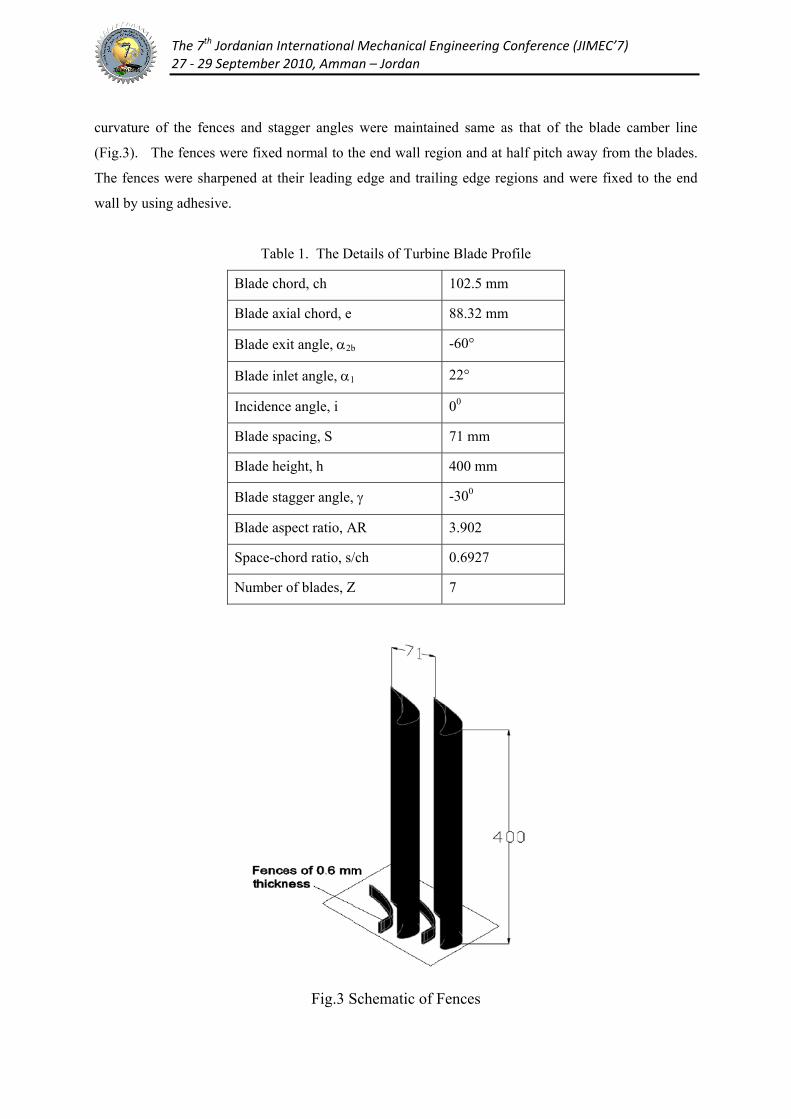
curvature of the fences and stagger angles were maintained same as that of the blade camber line

(Fig.3). The fences were fixed normal to the end wall region and at half pitch away from the blades.

The fences were sharpened at their leading edge and trailing edge regions and were fixed to the end

wall by using adhesive.

Table 1. The Details of Turbine Blade Profile

Blade chord, ch 102.5 mm

Blade axial chord, e 88.32 mm

Blade exit angle, α2b -60°

Blade inlet angle, α1 22°

Incidence angle, i 00

Blade spacing, S 71 mm

Blade height, h 400 mm

Blade stagger angle, γ -300

Blade aspect ratio, AR 3.902

Space-chord ratio, s/ch 0.6927

Number of blades, Z 7

Fig.3 Schematic of Fences


A traversing mechanism allowed the five-hole pressure probe (head diameter 2.4 mm) to move in

spanwise and pitchwise directions as well as in rotary motion about its longitudinal axis. A slot was

made normal to the cascade flow direction in top plate for the movement of traverse mechanism.

A digital type micro-manometer (type FC 012, Furness Controls Ltd., UK) together with a 20

channel scanning box (type FC 011, Furness Controls Ltd., UK) was used for recording the

pressures sensed by the miniature five-hole pressure probe. The scanning box facilitates reading 20

pressures sequentially without disturbing the connection of the sensor.

The probe was traversed in the spanwise direction from midspan to end wall region at 26 locations

with more measurement points in the end wall region. For each spanwise location, the probe was

traversed in the pitchwise direction at more than 25 locations covering one blade pitch. More readings

were obtained in the wake zone of the blade. For the present investigations, the flow studies were

made at the exit of the cascade as well as on the blade tip surface. Using total and static pressure

values along with the yaw and pitch angles, the flow velocity and its three components in axial,

pitchwise and spanwise directions were determined. The Reynolds number based on chord and exit

velocity was maintained at 1.5 x 105.

3. RESULTS AND DISCUSSION

The results obtained from the experimenal investigation on a two dimensional linear cascade using 82°

deflection turbine blades are presented and discussed. The results with a particular reference to

reduction in secondary losses in a turbine cascade using streamwise fences are highlighted.

Total Pressure Loss Coefficient

The local loss coefficient is calculated as the difference between midspan inlet total pressure (P01MS)

and local total pressure (P02) at each location downstream of the cascade, non-dimensionalised with

the dynamic pressure based on pitch and spanwise mass averaged velocity.

( )01MS 02local

22

2 p - pY =

Cρ (1)

The inlet total pressure was obtained at X/e = -0.4 and downstream survey was conducted at X/e =

1.06 where X is the distance in cascade axial direction and e is axial chord. X = 0.0 at the leading

edge of the blade and 1.0 at the trailing edge. As the two dimensionality of the flow was established

by Govardhan et al. [1994] for the same cascade, the flow survey was studied over one half of the


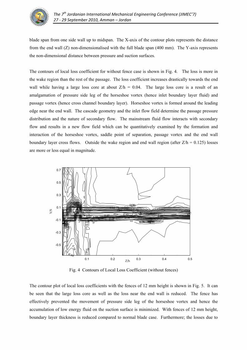
blade span from one side wall up to midspan. The X-axis of the contour plots represents the distance

from the end wall (Z) non-dimensionalised with the full blade span (400 mm). The Y-axis represents

the non-dimensional distance between pressure and suction surfaces.

The contours of local loss coefficient for without fence case is shown in Fig. 4. The loss is more in

the wake region than the rest of the passage. The loss coefficient increases drastically towards the end

wall while having a large loss core at about Z/h = 0.04. The large loss core is a result of an

amalgamation of pressure side leg of the horseshoe vortex (hence inlet boundary layer fluid) and

passage vortex (hence cross channel boundary layer). Horseshoe vortex is formed around the leading

edge near the end wall. The cascade geometry and the inlet flow field determine the passage pressure

distribution and the nature of secondary flow. The mainstream fluid flow interacts with secondary

flow and results in a new flow field which can be quantitatively examined by the formation and

interaction of the horseshoe vortex, saddle point of separation, passage vortex and the end wall

boundary layer cross flows. Outside the wake region and end wall region (after Z/h = 0.125) losses

are more or less equal in magnitude.

0.1 0.2 0.3 0.4 0.5Z/h

-0.5

-0.3

-0.1

0.1

0.3

0.5

0.7

Y/S

0.06

0.0

6 0.06

0.10

0.1

0 0

.10

0.1

0

0.10

0.15

0.15

0.15

0.19

0.19

0.19

0.24

0.24

0.24

0.28

0.28

0.33

0.33

0.37 0.37

0.42

0.42

0.46

0.46 0.51 0.51

0.5

6 0.56 0.56 0.60

0.60

0.65

0.69 0.7

4

0.78 0.83

Fig. 4 Contours of Local Loss Coefficient (without fences)

The contour plot of local loss coefficients with the fences of 12 mm height is shown in Fig. 5. It can

be seen that the large loss core as well as the loss near the end wall is reduced. The fence has

effectively prevented the movement of pressure side leg of the horseshoe vortex and hence the

accumulation of low energy fluid on the suction surface is minimized. With fences of 12 mm height,

boundary layer thickness is reduced compared to normal blade case. Furthermore; the losses due to


corner vortex are slightly reduced by the fences, as expected from the weakening of the end wall

cross-flow.

0.1 0.2 0.3 0.4 0.5Z/h

-0.5

-0.3

-0.1

0.1

0.3

0.5

0.7

Y/S

0.03

0.0

3 0.03

0.03

0.0

3

0.03 0.06

0.06

0.06

0.10

0.10

0.10 0.10

0.13

0.13

0.13

0.17

0.17

0.17

0.17

0.20

0.20

0.20

0.20

0.2

0

0.24

0.24

0.24 0.24

0.2

4

0.27

0.27

0.27

0.31

0.3

1

0.31

0.34 0.34

0.34

0.37 0.37

0.37

0.41 0.41

0.41

0.44 0.44

0.4

4 0.48

0.4

8 0.4

8 0.51 0.5

1

0.51

0.5

5 0.55

0.58

Fig. 5 Contours of Local Loss Coefficient with Fence of 12 mm Height

0.1 0.2 0.3 0.4 0.5Z/h

-0.5

-0.3

-0.1

0.1

0.3

0.5

0.7

Y/S 0.06

0.06

0.0

6

0.0

6

0.06

0.06

0.06

0.06

0.13

0.13

0.13

0.13

0.19

0.19

0.19

0.19

0.25

0.25

0.25

0.25

0.32

0.32

0.32

0.38

0.38 0.44

0.51 0.57

Fig. 6 Contours of Local Loss Coefficient with Fenced of 16 mm Height

The contour of local loss coefficients with fence of 16 mm height is plotted in the Fig. 6. The

contours are almost same as in the case with fence of 12 mm height. In this case the high loss core has

further reduced and it has split in to two small loss cores. The loss coefficient is reduced because of


reduction in the boundary layer thickness and resulting in overall reduction of loss in the end wall

region.

Using fences, the strength of the passage vortex and the loss associated with it has decreased. These

aspects are clearly seen when the pitchwise mass averaged total pressure loss coefficient is presented.

The local loss coefficients were pitchwise mass averaged, and the distribution of it along the span of

the blade is shown in Fig. 7. The losses are maximum slightly away from the end wall due to end

wall boundary layer. The end wall boundary layer loss is less when fences are incorporated. The loss

peak without fence case occurs at Z/h = 0.04 with a magnitude of 0.28. When the fences are fixed half

pitch away from the blades, the loss peak magnitude is reduced to 0.24, 0.19 for fence heights of 12

mm, and 16 mm respectively. With streamwise fences, the loss core not only reduced in magnitude

but also moved slightly away from the suction surface. The fences effectively prevented the

movement of pressure side leg of the horseshoe vortex and hence the accumulation of low energy fluid

on the suction surface is minimized. The fences are effective in preventing the vortex from growing to

its full strength and shifted the core of the vortex from the suction surface resulting in lesser

aerodynamic losses in the passage.

0.0 0.1 0.2 0.3 0.4 0.50.00

0.05

0.10

0.15

0.20

0.25

0.30

Loca

l Pre

ssur

e Lo

ss C

oeff

icie

nt, Y

Loca

l

Z/h

Without fences With Fences of 12 mm Height With Fences of 16 mm Height

Fig. 7 Spanwise Distribution of Pitchwise Mass Averaged Loss Coefficient


Exit Flow Angle

The blade angle at the inlet is 22° and at the exit angle is -60°. The exit angle increases close to end

wall. In a passage, whenever turning of fluid occurs, a balance is established between the static

pressure gradients and the centrifugal forces in the fluid. The pressure varies across the passage from

one surface of a blade to another surface of the nearest blade.

By radial equilibrium theory, it is assumed that for a turbine with annulus wall parallel to the axis, the

flow streamlines upstream and downstream of a blade row lie on concentric cylinders. Also a flow

radial shift takes places within the blade row. The relationship between the free stream velocity, radial

static pressure gradient and the radius of the curvature of the streamline gives required information

about the flow direction. The relationship can be written as

2

c

C dp = r dr

ρ (2)

Where C is freestream velocity and rc = radius of curvature

Towards the end wall, within the boundary layer, velocity decrease. The reduced kinetic energy

becomes insufficient to balance the imposed pressure gradient and the radius of curvature of

streamline becomes less resulting in overturning of the flow. The term ‘overturning’ is used to denote

the flow deflection, which is larger than the expected geometric deflection of the blade. If the flow

deflection is less than the geometric deflection of the blade, it is referred to as ‘underturning’.

The spanwise distribution of pitchwise mass averaged exit flow angles for all three cases (with and

without fences) is plotted in Fig. 8. The mass averaged angle for normal blade (without fences) case

overturns by about 7° on the end wall. The overturn is reduced to about 5° and 4° for fences of

heights 12 mm and 16 mm respectively. The amount of underturning in the region of loss core is

affected by the presence of fences. When the fences are incorporated, flow underturns more and the

midspan angle is also slightly reduced by the presence of fences. From spanwise distribution, the

flow angle has maximum slopes near the end wall region. The flow underturning decays faster

towards the midspan when the fences are incorporated.

Lift and Drag Coefficients

The local lift and drag coefficients are pitchwise mass averaged to get the spanwise distribution . The

variation of drag and lift coefficients along the span of the blade are plotted in Figs. 9 and 10. Figure


9 shows spanwise distribution of drag coefficient along the span of the blade. The drag coefficient is

more near the end wall for without fences, compared to fences height of 12 mm & 16 mm

respectively. The peak without fences occurs at Z/h = 0.04 with a magnitude of 0.21. The peak

reduces to 0.16, 0.15 for fences heights of 12 mm, and 16 mm respectively. Reduction in total

pressure losses with fences is primary reason for the reduction in drag coefficient. The drag

coefficient is more in the loss core region. From Fig. 10, it is clear that the lift coefficient is

significantly less in the boundary layer. Near the wall CD is very high, hence CL is expected to be less.

The lift coefficient gradually increases from the end wall and remains more or less constant after about

Z/h=0.09.

0.0 0.1 0.2 0.3 0.4 0.5

56

58

60

62

64

66

Exit

Flow

Ang

le

Z/h

without fencewith fences of 12 mm heightwith fences of 16 mm height

Fig. 8 Spanwise Distribution of Pitchwise Mass Averaged Exit Flow Angle

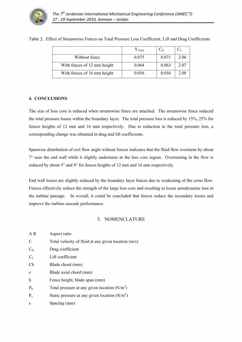
The overall effect of streamwise fence on reduction of total losses is shown in the following table.

The total loss is reduced by 15%, 25% for fences heights of 12 mm and 16 mm respectively compared

to without fence case. Due to reduction in the total pressure loss, a corresponding change is obtained

in drag and lift coefficients.


0.0 0.1 0.2 0.3 0.4 0.50.02

0.04

0.06

0.08

0.10

0.12

0.14

0.16

0.18

0.20

0.22

Dra

g C

oeff

icie

nt, C

D

Z/h

without fences with fences of 12 mm height with fences of 16 mm height

Fig. 9 Spanwise Distribution of Pitchwise Mass Averaged Drag Coefficient

0.0 0.1 0.2 0.3 0.4 0.51.85

1.90

1.95

2.00

2.05

2.10

2.15

Lift

Coe

ffic

ient

, CL

Z/h

withpot fencewith fences of 12 mm height with fences of 16 mm heigh

Fig. 10 Spanwise Distribution of Pitchwise Mass Averaged Lift Coefficient


Table 2. Effect of Streamwise Fences on Total Pressure Loss Coefficient, Lift and Drag Coefficients

YTotal CD CL

Without fence 0.075 0.071 2.06

With fences of 12 mm height 0.064 0.063 2.07

With fences of 16 mm height 0.056 0.056 2.08

4. CONCLUSIONS

The size of loss core is reduced when streamwise fence are attached. The streamwise fence reduced

the total pressure losses within the boundary layer. The total pressure loss is reduced by 15%, 25% for

fences heights of 12 mm and 16 mm respectively. Due to reduction in the total pressure loss, a

corresponding change was obtained in drag and lift coefficients.

Spanwise distribution of exit flow angle without fences indicates that the fluid flow overturns by about

7° near the end wall while it slightly underturns in the loss core region. Overturning in the flow is

reduced by about 5° and 4° for fences heights of 12 mm and 16 mm respectively.

End wall losses are slightly reduced by the boundary layer fences due to weakening of the cross flow.

Fences effectively reduce the strength of the large loss core and resulting in lesser aerodynamic loss in

the turbine passage. In overall, it could be concluded that fences reduce the secondary losses and

improve the turbine cascade performance.

5. NOMENCLATURE

A R Aspect ratio

C Total velocity of fluid at any given location (m/s)

CD Drag coefficient

CL Lift coefficient

Ch Blade chord (mm)

e Blade axial chord (mm)

h Fence height, blade span (mm)

P0 Total pressure at any given location (N/m2)

Ps Static pressure at any given location (N/m2)

s Spacing (mm)


X Distance along the cascade flow direction (mm)

Y Distance normal to the cascade flow direction (mm)

YLocal Local pressure loss coefficient

Z Longitudinal distance along the span of the blade (mm)

α1 Blade inlet angle (deg.)

α2b Blade exit angle (deg.)

γ Stagger angle (deg.)

6. REFERENCES

1. Kawai, T., (1994), “ Effect of combined boundary layer fences on turbine secondary flow and

losses”, JSME International Journal 37, 377-384.

2. Moon, Y. J. and Koh, S. R., (2001), “ Counter rotating streamwise vortex formation in the turbine

cascade with endwall fence”, Computer & Fluids 30, 473-490.

3. Aunapu, N V., Volino, R J., Flack, K A., and Stoddard, R. M., (2000), “Secondary flow

measurements in a turbine passage with end wall flow modification”, ASME J. of Turbomachinery

122, 651-658.

4. Govardhan, M., Rajender, A., and Umang, J. P., (2006), “ Effect of streamwise fences

on secondary flows and losses in a two-dimensional turbine rotor cascade” Journal of Thermal

Science 15, 296-305.

5. Chung J. T. & Simon T. W., (1993), “Effectiveness of the gas turbine endwall fences in

secondary flow control at elevated freestream turbulence levels”, ASME Paper No. 93-GT-51.

6. Govardhan, M., Venkatrayulu, N., and Vishnubhotla, V.S., (1994), “Influence of tip

clearance on the inter blade and exit flow field of a turbine rotor cascade", 39th ASME-

International Gas Turbine and Aeroengine Congress The Netherlands, Hague, pp. 1-8, (94-

GT-359).

Date post:	13-May-2018
Category:	Documents
Upload:	ledang
View:	220 times
Download:	1 times

SECONDARY LOSS REDUCTION BY STREAMWISE FENCES …€¦ · SECONDARY LOSS REDUCTION BY STREAMWISE...

Documents