ENGR 202 – Electrical Fundamentals II

SECTION 1: SINUSOIDAL STEADY-STATE ANALYSIS

K. Webb ENGR 202

Sinusoids2

K. Webb ENGR 202

3

Sinusoidal Signals

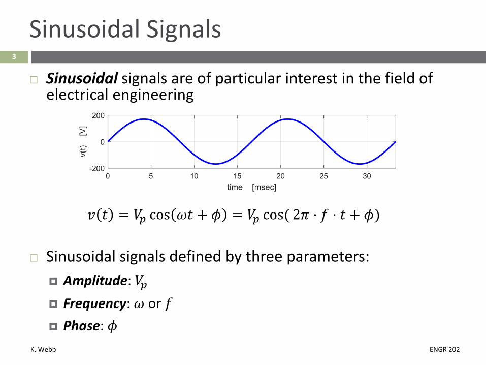
Sinusoidal signals are of particular interest in the field of electrical engineering

𝑣𝑣 𝑡𝑡 = 𝑉𝑉𝑝𝑝 cos 𝜔𝜔𝑡𝑡 + 𝜙𝜙 = 𝑉𝑉𝑝𝑝 cos(2𝜋𝜋 ⋅ 𝑓𝑓 ⋅ 𝑡𝑡 + 𝜙𝜙)

Sinusoidal signals defined by three parameters: Amplitude: 𝑉𝑉𝑝𝑝 Frequency: 𝜔𝜔 or 𝑓𝑓 Phase: 𝜙𝜙

K. Webb ENGR 202

4

Amplitude

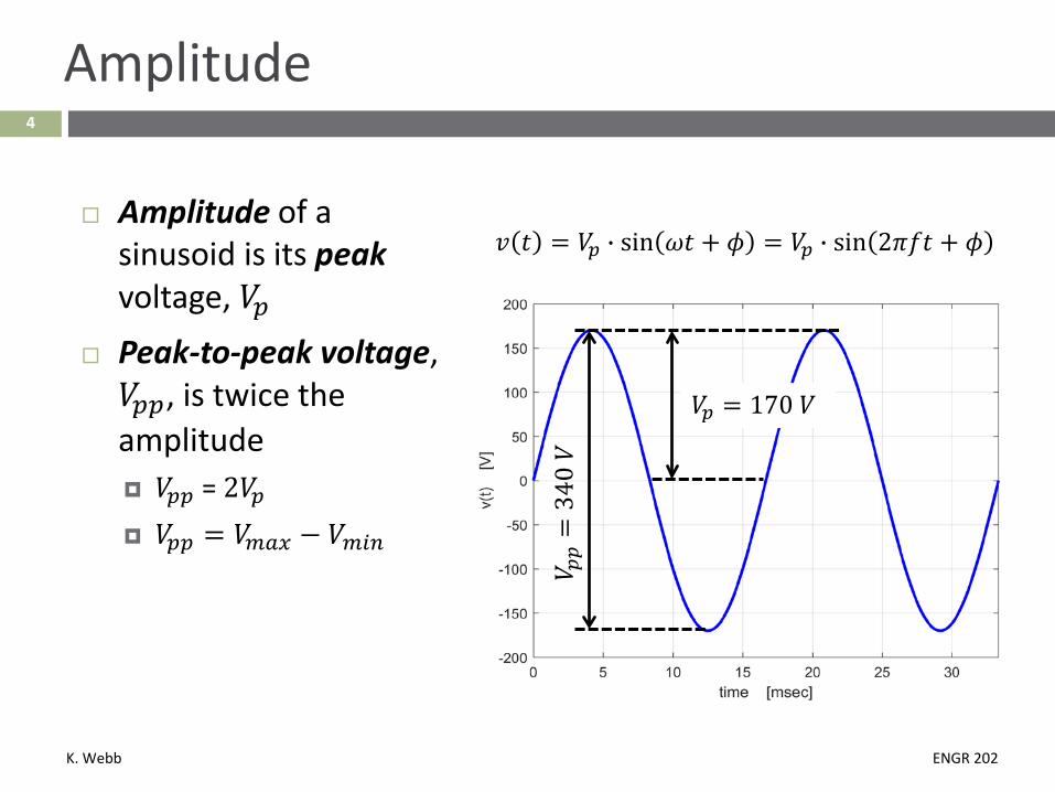
Amplitude of a sinusoid is its peakvoltage, 𝑉𝑉𝑝𝑝

Peak-to-peak voltage, 𝑉𝑉𝑝𝑝𝑝𝑝, is twice the amplitude 𝑉𝑉𝑝𝑝𝑝𝑝 = 2𝑉𝑉𝑝𝑝 𝑉𝑉𝑝𝑝𝑝𝑝 = 𝑉𝑉𝑚𝑚𝑚𝑚𝑚𝑚 − 𝑉𝑉𝑚𝑚𝑚𝑚𝑚𝑚

𝑣𝑣 𝑡𝑡 = 𝑉𝑉𝑝𝑝 � sin 𝜔𝜔𝑡𝑡 + 𝜙𝜙 = 𝑉𝑉𝑝𝑝 � sin 2𝜋𝜋𝑓𝑓𝑡𝑡 + 𝜙𝜙

𝑉𝑉𝑝𝑝 = 170 𝑉𝑉

𝑉𝑉 𝑝𝑝𝑝𝑝

=34

0𝑉𝑉

K. Webb ENGR 202

5

Frequency

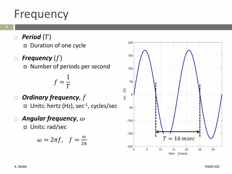
Period (𝑇𝑇) Duration of one cycle

Frequency (𝑓𝑓) Number of periods per second

𝑓𝑓 =1𝑇𝑇

Ordinary frequency, 𝑓𝑓 Units: hertz (Hz), sec-1, cycles/sec

Angular frequency, 𝜔𝜔 Units: rad/sec

𝜔𝜔 = 2𝜋𝜋𝑓𝑓, 𝑓𝑓 = 𝜔𝜔2𝜋𝜋

𝑇𝑇 = 16 𝑚𝑚𝑚𝑚𝑚𝑚𝑚𝑚

K. Webb ENGR 202

6

Phase

Phase Angular constant in signal expression, 𝜙𝜙

𝑣𝑣 𝑡𝑡 = 𝑉𝑉𝑝𝑝 sin 𝜔𝜔𝑡𝑡 + 𝜙𝜙 Requires a time reference

Interested in relative, not absolute, phase

Here, 𝑣𝑣1 𝑡𝑡 leads 𝑣𝑣2 𝑡𝑡 𝑣𝑣2 𝑡𝑡 lags 𝑣𝑣1 𝑡𝑡

Units: radians Not technically correct, but OK

to express in degrees, e.g.:

𝑣𝑣 𝑡𝑡 = 170 𝑉𝑉 sin 2𝜋𝜋 ⋅ 60𝐻𝐻𝐻𝐻 ⋅ 𝑡𝑡 + 34°

K. Webb ENGR 202

7

Sinusoidal Steady-State Analysis

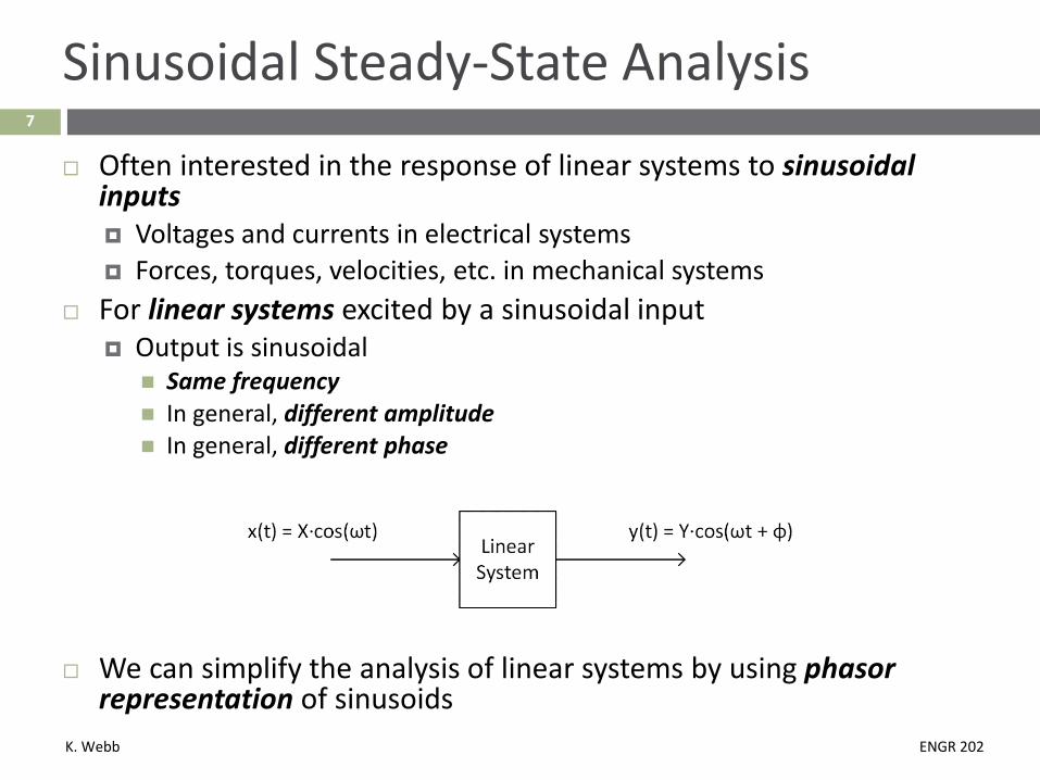
Often interested in the response of linear systems to sinusoidal inputs Voltages and currents in electrical systems Forces, torques, velocities, etc. in mechanical systems

For linear systems excited by a sinusoidal input Output is sinusoidal

Same frequency In general, different amplitude In general, different phase

We can simplify the analysis of linear systems by using phasor representation of sinusoids

K. Webb ENGR 202

8

Phasors

Phasor A complex number representing the amplitude and

phase of a sinusoidal signal Frequency is not included Remains constant and is accounted for separately System characteristics (frequency-dependent) evaluated at

the frequency of interest as first step in the analysis

Phasors are complex numbers Before applying phasors to the analysis of electrical

circuits, we’ll first review the properties of complex numbers

K. Webb ENGR 202

Complex Numbers9

K. Webb ENGR 202

10

Complex Numbers

A complex number can be represented as

𝐻𝐻 = 𝑥𝑥 + 𝑗𝑗𝑗𝑗

𝑥𝑥: real part (a real number) 𝑗𝑗: imaginary part (a real number) 𝑗𝑗 = −1 is the imaginary unit

Complex numbers can be represented three ways: Cartesian form: 𝐻𝐻 = 𝑥𝑥 + 𝑗𝑗𝑗𝑗 Polar form: 𝐻𝐻 = 𝑟𝑟𝑟𝜙𝜙 Exponential form: 𝐻𝐻 = 𝑟𝑟𝑚𝑚𝑗𝑗𝑗𝑗

K. Webb ENGR 202

11

Complex Numbers as Vectors

A complex number can be represented as a vector in the complex plane

Complex plane Real axis – horizontal Imaginary axis – vertical

A vector from the origin to 𝐻𝐻 Real part, 𝑥𝑥 Imaginary part, 𝑗𝑗

𝐻𝐻 = 𝑥𝑥 + 𝑗𝑗𝑗𝑗

Vector has a magnitude, 𝑟𝑟 And an angle, 𝜃𝜃

𝐻𝐻 = 𝑟𝑟𝑟𝜃𝜃

K. Webb ENGR 202

12

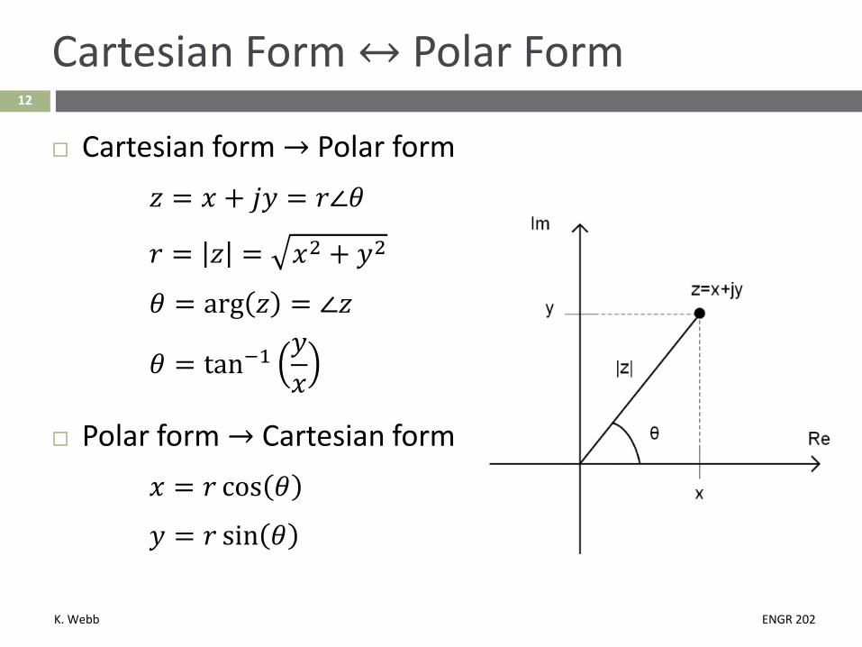
Cartesian Form ↔ Polar Form

Cartesian form → Polar form𝐻𝐻 = 𝑥𝑥 + 𝑗𝑗𝑗𝑗 = 𝑟𝑟𝑟𝜃𝜃

𝑟𝑟 = 𝐻𝐻 = 𝑥𝑥2 + 𝑗𝑗2

𝜃𝜃 = arg 𝐻𝐻 = 𝑟𝐻𝐻

𝜃𝜃 = tan−1𝑗𝑗𝑥𝑥

Polar form → Cartesian form𝑥𝑥 = 𝑟𝑟 cos 𝜃𝜃

𝑗𝑗 = 𝑟𝑟 sin 𝜃𝜃

K. Webb ENGR 202

13

Complex Numbers – Addition/Subtraction

Addition and subtraction of complex numbers Best done in Cartesian form Real parts add/subtract Imaginary parts add/subtract

For example:𝐻𝐻1 = 𝑥𝑥1 + 𝑗𝑗𝑗𝑗1𝐻𝐻2 = 𝑥𝑥2 + 𝑗𝑗𝑗𝑗2𝐻𝐻1 + 𝐻𝐻2 = 𝑥𝑥1 + 𝑥𝑥2 + 𝑗𝑗 𝑗𝑗1 + 𝑗𝑗2𝐻𝐻1 − 𝐻𝐻2 = 𝑥𝑥1 − 𝑥𝑥2 + 𝑗𝑗 𝑗𝑗1 − 𝑗𝑗2

K. Webb ENGR 202

14

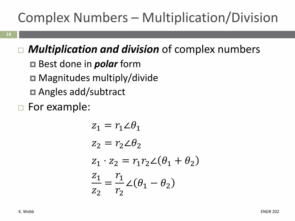
Complex Numbers – Multiplication/Division

Multiplication and division of complex numbers Best done in polar form Magnitudes multiply/divide Angles add/subtract

For example:𝐻𝐻1 = 𝑟𝑟1𝑟𝜃𝜃1𝐻𝐻2 = 𝑟𝑟2𝑟𝜃𝜃2𝐻𝐻1 ⋅ 𝐻𝐻2 = 𝑟𝑟1𝑟𝑟2𝑟 𝜃𝜃1 + 𝜃𝜃2𝐻𝐻1𝐻𝐻2

=𝑟𝑟1𝑟𝑟2𝑟 𝜃𝜃1 − 𝜃𝜃2

K. Webb ENGR 202

15

Complex Conjugate

Conjugate of a complex number Number that results from

negating the imaginary part

𝐻𝐻 = 𝑥𝑥 + 𝑗𝑗𝑗𝑗𝐻𝐻∗ = 𝑥𝑥 − 𝑗𝑗𝑗𝑗

Or, equivalently, from negating the angle

𝐻𝐻 = 𝑟𝑟𝑟𝜃𝜃

𝐻𝐻∗ = 𝑟𝑟𝑟 − 𝜃𝜃

K. Webb ENGR 202

16

Complex Fractions

Multiplying a number by its complex conjugate yields the squared magnitude of that number A real number

𝐻𝐻 ⋅ 𝐻𝐻∗ = 𝑥𝑥 + 𝑗𝑗𝑗𝑗 𝑥𝑥 − 𝑗𝑗𝑗𝑗 = 𝑥𝑥2 + 𝑗𝑗2

𝐻𝐻 ⋅ 𝐻𝐻∗ = 𝑟𝑟𝑟𝜃𝜃 ⋅ 𝑟𝑟𝑟 − 𝜃𝜃 = 𝑟𝑟2𝑟𝜃𝜃 − 𝜃𝜃 = 𝑟𝑟2

Rationalizing the denominator of a complex fraction: Multiply numerator and denominator by the complex conjugate

of the denominator

𝐻𝐻 =𝑥𝑥1 + 𝑗𝑗𝑗𝑗1𝑥𝑥2 + 𝑗𝑗𝑗𝑗2

⋅𝑥𝑥2 − 𝑗𝑗𝑗𝑗2𝑥𝑥2 − 𝑗𝑗𝑗𝑗2

𝐻𝐻 =𝑥𝑥1𝑥𝑥2 + 𝑗𝑗1𝑗𝑗2𝑥𝑥22 + 𝑗𝑗22

+ 𝑗𝑗𝑥𝑥2𝑗𝑗1 − 𝑥𝑥1𝑗𝑗2𝑥𝑥22 + 𝑗𝑗22

K. Webb ENGR 202

17

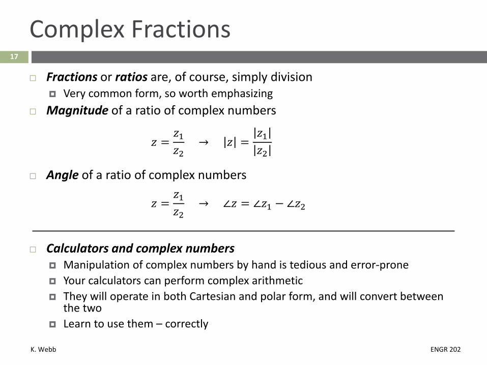
Complex Fractions

Fractions or ratios are, of course, simply division Very common form, so worth emphasizing

Magnitude of a ratio of complex numbers

𝐻𝐻 =𝐻𝐻1𝐻𝐻2

→ 𝐻𝐻 =𝐻𝐻1𝐻𝐻2

Angle of a ratio of complex numbers

𝐻𝐻 =𝐻𝐻1𝐻𝐻2

→ 𝑟𝐻𝐻 = 𝑟𝐻𝐻1 − 𝑟𝐻𝐻2

Calculators and complex numbers Manipulation of complex numbers by hand is tedious and error-prone Your calculators can perform complex arithmetic They will operate in both Cartesian and polar form, and will convert between

the two Learn to use them – correctly

K. Webb ENGR 202

Phasors18

K. Webb ENGR 202

19

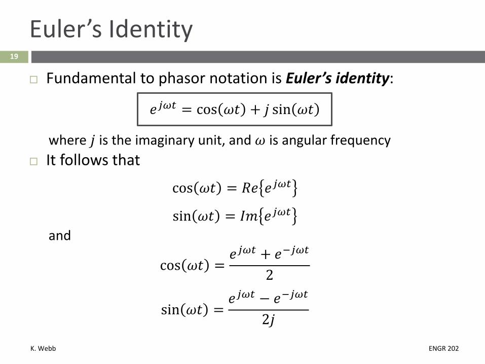
Euler’s Identity

Fundamental to phasor notation is Euler’s identity:

𝑚𝑚𝑗𝑗𝜔𝜔𝑗𝑗 = cos 𝜔𝜔𝑡𝑡 + 𝑗𝑗 sin 𝜔𝜔𝑡𝑡

where 𝑗𝑗 is the imaginary unit, and 𝜔𝜔 is angular frequency It follows that

cos 𝜔𝜔𝑡𝑡 = 𝑅𝑅𝑚𝑚 𝑚𝑚𝑗𝑗𝜔𝜔𝑗𝑗

sin 𝜔𝜔𝑡𝑡 = 𝐼𝐼𝑚𝑚 𝑚𝑚𝑗𝑗𝜔𝜔𝑗𝑗

and

cos 𝜔𝜔𝑡𝑡 =𝑚𝑚𝑗𝑗𝜔𝜔𝑗𝑗 + 𝑚𝑚−𝑗𝑗𝜔𝜔𝑗𝑗

2

sin 𝜔𝜔𝑡𝑡 =𝑚𝑚𝑗𝑗𝜔𝜔𝑗𝑗 − 𝑚𝑚−𝑗𝑗𝜔𝜔𝑗𝑗

2𝑗𝑗

K. Webb ENGR 202

20

Phasors

Consider a sinusoidal voltage𝑣𝑣 𝑡𝑡 = 𝑉𝑉𝑝𝑝 cos 𝜔𝜔𝑡𝑡 + 𝜙𝜙

Using Euler’s identity, we can represent this as

𝑣𝑣 𝑡𝑡 = 𝑅𝑅𝑚𝑚 𝑉𝑉𝑝𝑝𝑚𝑚𝑗𝑗 𝜔𝜔𝑗𝑗+𝑗𝑗 = 𝑅𝑅𝑚𝑚 𝑉𝑉𝑝𝑝𝑚𝑚𝑗𝑗𝑗𝑗𝑚𝑚𝑗𝑗𝜔𝜔𝑗𝑗

where 𝑉𝑉𝑝𝑝 represents magnitude 𝑚𝑚𝑗𝑗𝑗𝑗 represents phase 𝑚𝑚𝑗𝑗𝜔𝜔𝑗𝑗 represents a sinusoid of frequency 𝜔𝜔

Grouping the first two terms together, we have

𝑣𝑣 𝑡𝑡 = 𝑅𝑅𝑚𝑚 𝐕𝐕𝑚𝑚𝑗𝑗𝜔𝜔𝑗𝑗

where 𝐕𝐕 is the phasor representation of 𝑣𝑣 𝑡𝑡

K. Webb ENGR 202

21

Phasors

𝑣𝑣 𝑡𝑡 = 𝑅𝑅𝑚𝑚 𝐕𝐕𝑚𝑚𝑗𝑗𝜔𝜔𝑗𝑗

The phasor representation of 𝑣𝑣 𝑡𝑡

𝐕𝐕 = 𝑉𝑉𝑝𝑝𝑚𝑚𝑗𝑗𝑗𝑗

A representation of magnitude and phase only Time-harmonic portion (𝑚𝑚𝑗𝑗𝜔𝜔𝑗𝑗) has been dropped

Phasors greatly simplify sinusoidal steady-state analysis Messy trigonometric functions are eliminated Differentiation and integration transformed to algebraic operations

Time-domain representation:

𝑣𝑣 𝑡𝑡 = 𝑉𝑉𝑝𝑝 sin 𝜔𝜔𝑡𝑡 + 𝜙𝜙

Phasor-domain representation:

𝐕𝐕 = 𝑉𝑉𝑝𝑝𝑚𝑚𝑗𝑗𝑗𝑗 = 𝑉𝑉𝑝𝑝𝑟𝜙𝜙

K. Webb ENGR 202

22

Voltage & Current in the Phasor Domain

We will use phasors to simplify analysis of electrical circuits Need an understanding of electrical component behavior in the phasor domain Relationships between voltage phasors and current phasors for Rs, Ls, and Cs

Resistor Voltage across a resistor given by

𝑣𝑣 𝑡𝑡 = 𝑖𝑖 𝑡𝑡 𝑅𝑅

𝑖𝑖 𝑡𝑡 = 𝐼𝐼𝑝𝑝 cos 𝜔𝜔𝑡𝑡 + 𝜙𝜙

Converting to phasor form

𝐕𝐕 = 𝐼𝐼𝑝𝑝𝑚𝑚𝑗𝑗𝑗𝑗 𝑅𝑅

𝐕𝐕 = 𝐈𝐈𝑅𝑅 𝐈𝐈 =𝐕𝐕R

Ohm’s law in phasor form

K. Webb ENGR 202

23

V-I Relationships in the Phasor Domain

Capacitor Current through the capacitor given by

𝑖𝑖 𝑡𝑡 = 𝐶𝐶𝑑𝑑𝑣𝑣𝑑𝑑𝑡𝑡

𝑖𝑖 𝑡𝑡 = 𝐶𝐶𝑑𝑑𝑑𝑑𝑡𝑡 𝑉𝑉𝑝𝑝 cos 𝜔𝜔𝑡𝑡 + 𝜙𝜙

𝑖𝑖 𝑡𝑡 = −𝜔𝜔𝐶𝐶𝑉𝑉𝑝𝑝 sin 𝜔𝜔𝑡𝑡 + 𝜙𝜙

Applying a trig identity:

− sin 𝐴𝐴 = cos 𝐴𝐴 + 90°gives

𝑖𝑖 𝑡𝑡 = 𝜔𝜔𝐶𝐶𝑉𝑉𝑝𝑝 cos 𝜔𝜔𝑡𝑡 + 𝜙𝜙 + 90°

Converting to phasor form

𝐈𝐈 = 𝜔𝜔𝐶𝐶𝑉𝑉𝑝𝑝𝑚𝑚𝑗𝑗 𝑗𝑗+90° = 𝜔𝜔𝐶𝐶𝑉𝑉𝑝𝑝𝑚𝑚𝑗𝑗𝑗𝑗𝑚𝑚𝑗𝑗90°

K. Webb ENGR 202

24

V-I Relationships - Capacitor

Current phasor

𝐈𝐈 = 𝜔𝜔𝐶𝐶𝑉𝑉𝑝𝑝𝑚𝑚𝑗𝑗 𝑗𝑗+90° = 𝜔𝜔𝐶𝐶𝑉𝑉𝑝𝑝𝑚𝑚𝑗𝑗𝑗𝑗𝑚𝑚𝑗𝑗90°

Voltage phasor is

𝐕𝐕 = 𝑉𝑉𝑝𝑝𝑚𝑚𝑗𝑗𝑗𝑗

so𝐈𝐈 = 𝜔𝜔𝐶𝐶𝐕𝐕𝑚𝑚𝑗𝑗90°

Recognizing that 𝑚𝑚𝑗𝑗90° = 𝑗𝑗, we have

𝐈𝐈 = 𝑗𝑗𝜔𝜔𝐶𝐶𝐕𝐕 𝐕𝐕 =1𝑗𝑗𝜔𝜔𝐶𝐶

𝐈𝐈

K. Webb ENGR 202

25

V-I Relationships - Inductor

Inductor Voltage across an inductor given by

𝑣𝑣 𝑡𝑡 = 𝐿𝐿𝑑𝑑𝑖𝑖𝑑𝑑𝑡𝑡

𝑣𝑣 𝑡𝑡 = 𝐿𝐿𝑑𝑑𝑑𝑑𝑡𝑡

𝐼𝐼𝑝𝑝 cos 𝜔𝜔𝑡𝑡 + 𝜙𝜙

𝑣𝑣 𝑡𝑡 = −𝜔𝜔𝐿𝐿𝐼𝐼𝑝𝑝 sin 𝜔𝜔𝑡𝑡 + 𝜙𝜙 = 𝜔𝜔𝐿𝐿𝐼𝐼𝑝𝑝 cos 𝜔𝜔𝑡𝑡 + 𝜙𝜙 + 90°

Converting to phasor form

𝐕𝐕 = 𝜔𝜔𝐿𝐿𝐼𝐼𝑝𝑝𝑚𝑚𝑗𝑗 𝑗𝑗+90° = 𝜔𝜔𝐿𝐿𝐼𝐼𝑝𝑝𝑚𝑚𝑗𝑗𝑗𝑗𝑚𝑚𝑗𝑗90°

Again, recognizing that 𝑚𝑚𝑗𝑗90° = 𝑗𝑗, gives

𝐕𝐕 = 𝑗𝑗𝜔𝜔𝐿𝐿𝐈𝐈 𝐈𝐈 =1𝑗𝑗𝜔𝜔𝐿𝐿

𝐕𝐕

K. Webb ENGR 202

Impedance26

K. Webb ENGR 202

27

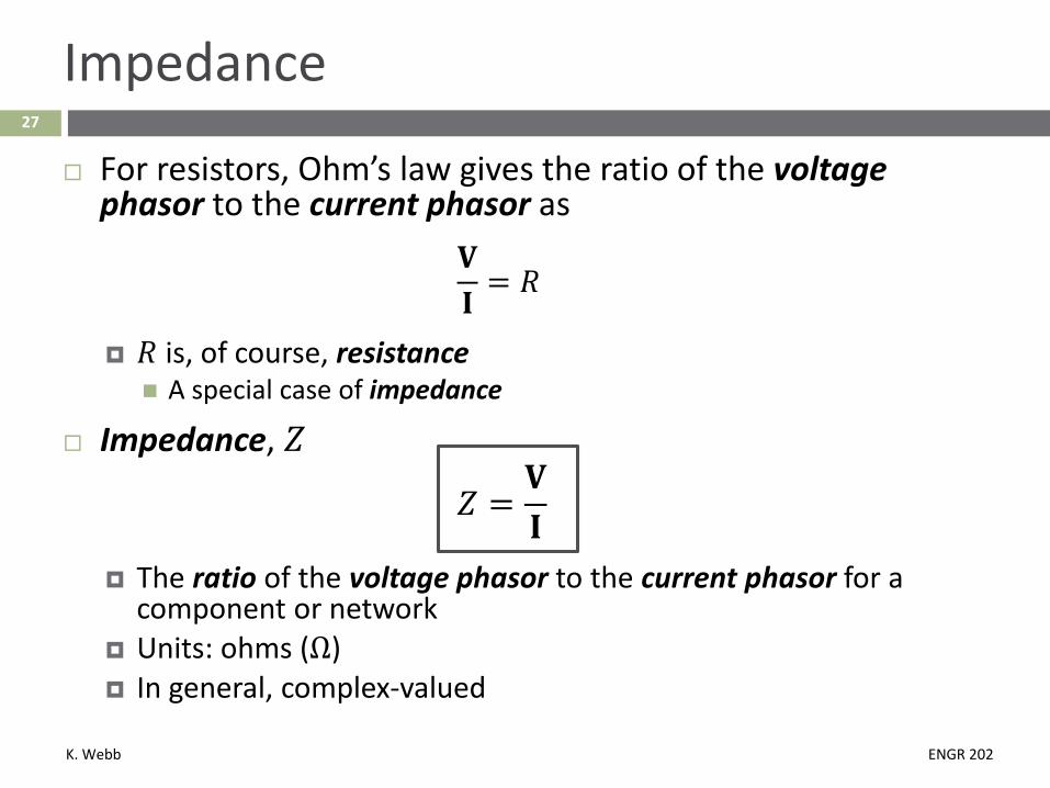
Impedance

For resistors, Ohm’s law gives the ratio of the voltage phasor to the current phasor as

𝐕𝐕𝐈𝐈 = 𝑅𝑅

𝑅𝑅 is, of course, resistance A special case of impedance

Impedance, 𝑍𝑍

𝑍𝑍 =𝐕𝐕𝐈𝐈

The ratio of the voltage phasor to the current phasor for a component or network

Units: ohms (Ω) In general, complex-valued

K. Webb ENGR 202

28

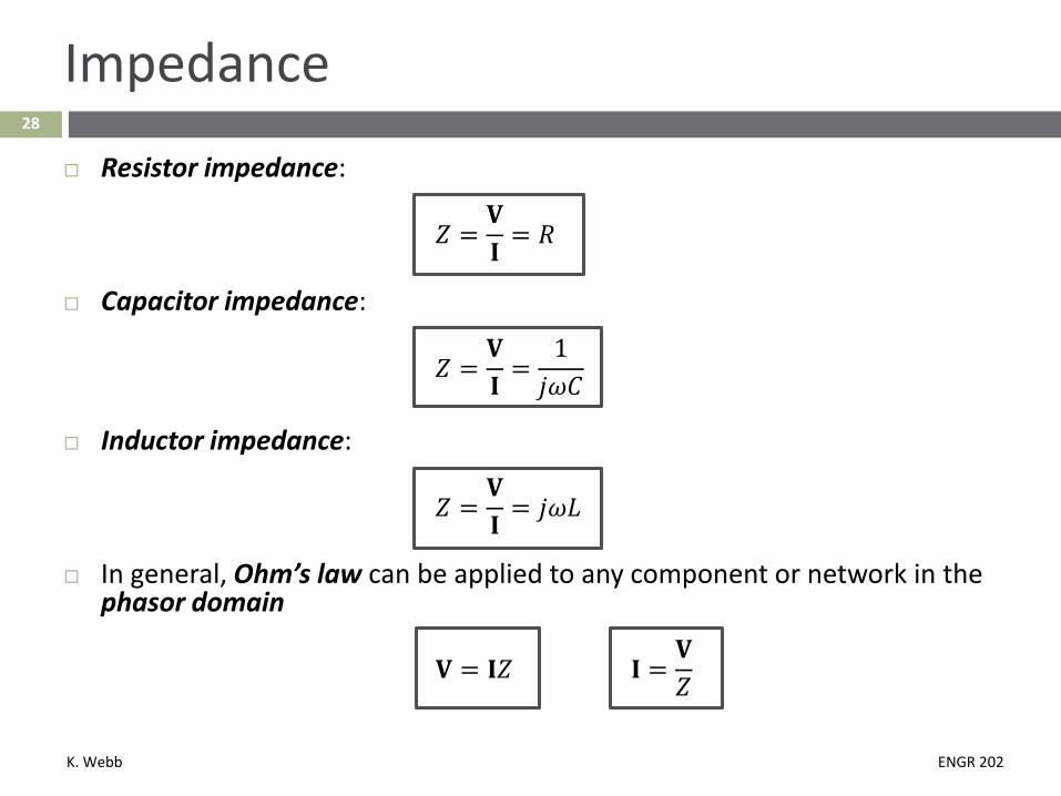
Impedance

Resistor impedance:

𝑍𝑍 =𝐕𝐕𝐈𝐈

= 𝑅𝑅

Capacitor impedance:

𝑍𝑍 =𝐕𝐕𝐈𝐈

=1𝑗𝑗𝜔𝜔𝐶𝐶

Inductor impedance:

𝑍𝑍 =𝐕𝐕𝐈𝐈 = 𝑗𝑗𝜔𝜔𝐿𝐿

In general, Ohm’s law can be applied to any component or network in the phasor domain

𝐕𝐕 = 𝐈𝐈𝑍𝑍 𝐈𝐈 =𝐕𝐕𝑍𝑍

K. Webb ENGR 202

Capacitor Impedance29

K. Webb ENGR 202

30

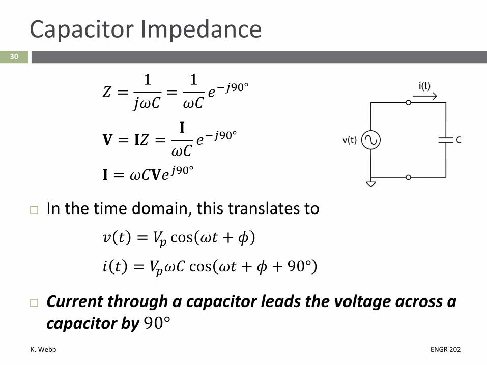
Capacitor Impedance

𝑍𝑍 =1𝑗𝑗𝜔𝜔𝐶𝐶

=1𝜔𝜔𝐶𝐶

𝑚𝑚−𝑗𝑗90°

𝐕𝐕 = 𝐈𝐈𝑍𝑍 =𝐈𝐈𝜔𝜔𝐶𝐶

𝑚𝑚−𝑗𝑗90°

𝐈𝐈 = 𝜔𝜔𝐶𝐶𝐕𝐕𝑚𝑚𝑗𝑗90°

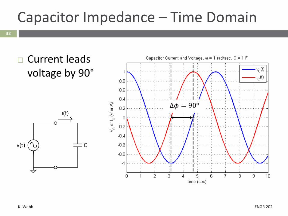
In the time domain, this translates to𝑣𝑣 𝑡𝑡 = 𝑉𝑉𝑝𝑝 cos 𝜔𝜔𝑡𝑡 + 𝜙𝜙

𝑖𝑖 𝑡𝑡 = 𝑉𝑉𝑝𝑝𝜔𝜔𝐶𝐶 cos 𝜔𝜔𝑡𝑡 + 𝜙𝜙 + 90°

Current through a capacitor leads the voltage across a capacitor by 90°

K. Webb ENGR 202

31

Capacitor Impedance – Phasor Diagram

Phasor diagram for a capacitor Voltage and current

phasors drawn as vectors in the complex plane

Current always leads voltage by 90°

K. Webb ENGR 202

32

Capacitor Impedance – Time Domain

Current leads voltage by 90°

Δ𝜙𝜙 = 90°

K. Webb ENGR 202

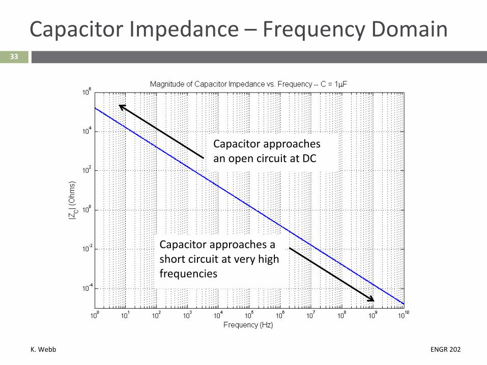
33

Capacitor Impedance – Frequency Domain

Capacitor approaches an open circuit at DC

Capacitor approaches a short circuit at very high frequencies

K. Webb ENGR 202

Inductor Impedance34

K. Webb ENGR 202

35

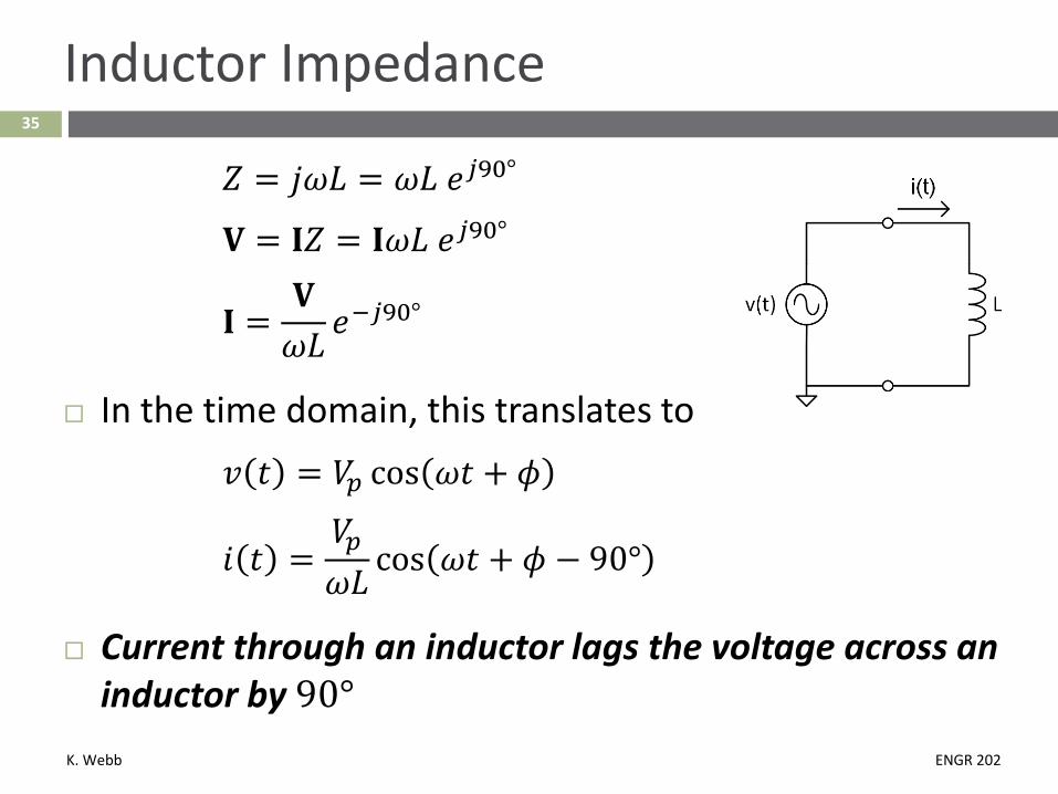
Inductor Impedance

𝑍𝑍 = 𝑗𝑗𝜔𝜔𝐿𝐿 = 𝜔𝜔𝐿𝐿 𝑚𝑚𝑗𝑗90°

𝐕𝐕 = 𝐈𝐈𝑍𝑍 = 𝐈𝐈𝜔𝜔𝐿𝐿 𝑚𝑚𝑗𝑗90°

𝐈𝐈 =𝐕𝐕𝜔𝜔𝐿𝐿

𝑚𝑚−𝑗𝑗90°

In the time domain, this translates to𝑣𝑣 𝑡𝑡 = 𝑉𝑉𝑝𝑝 cos 𝜔𝜔𝑡𝑡 + 𝜙𝜙

𝑖𝑖 𝑡𝑡 =𝑉𝑉𝑝𝑝𝜔𝜔𝐿𝐿

cos 𝜔𝜔𝑡𝑡 + 𝜙𝜙 − 90°

Current through an inductor lags the voltage across an inductor by 90°

K. Webb ENGR 202

36

Inductor Impedance – Phasor Diagram

Phasor diagram for an inductor Voltage and current

phasors drawn as vectors in the complex plane

Current always lags voltage by 90°

K. Webb ENGR 202

37

Inductor Impedance – Time Domain

Current lags voltage by 90°

Δ𝜙𝜙 = 90°

K. Webb ENGR 202

38

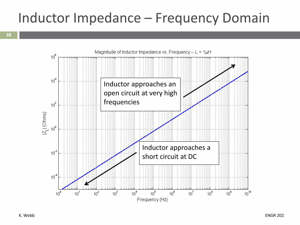
Inductor Impedance – Frequency Domain

Inductor approaches a short circuit at DC

Inductor approaches an open circuit at very high frequencies

K. Webb ENGR 202

39

Summary

Capacitor Impedance:

𝑍𝑍𝑐𝑐 =1𝑗𝑗𝜔𝜔𝐶𝐶

V-I phase relationship:

Current leads voltage by 90°

𝑣𝑣 𝑡𝑡 = 𝑉𝑉𝑝𝑝 cos 𝜔𝜔𝑡𝑡

𝑖𝑖 𝑡𝑡 = 𝑉𝑉𝑝𝑝𝜔𝜔𝐶𝐶 cos 𝜔𝜔𝑡𝑡 + 90°

Inductor Impedance:

𝑍𝑍𝐿𝐿 = 𝑗𝑗𝜔𝜔𝐿𝐿

V-I phase relationship:

Current lags voltage by 90°

𝑣𝑣 𝑡𝑡 = 𝑉𝑉𝑝𝑝 cos 𝜔𝜔𝑡𝑡

𝑖𝑖 𝑡𝑡 =𝑉𝑉𝑝𝑝𝜔𝜔𝐿𝐿

cos 𝜔𝜔𝑡𝑡 − 90°

K. Webb ENGR 202

40

ELI the ICE Man

Mnemonic for phase relation between current (I) and voltage (E) in inductors (L) and capacitors (C)

E L I the manI C EVoltage

leads current in an inductor

Current leads voltage

in a capacitor

K. Webb ENGR 202

Example Problems41

K. Webb ENGR 202

Convert each of the following time-domain signals to phasor form.

𝑣𝑣 𝑡𝑡 = 6𝑉𝑉 ⋅ cos 2𝜋𝜋 ⋅ 8𝑘𝑘𝐻𝐻𝐻𝐻 ⋅ 𝑡𝑡 + 12°

𝑖𝑖 𝑡𝑡 = 200𝑚𝑚𝐴𝐴 ⋅ sin 100 ⋅ 𝑡𝑡 − 38°

K. Webb ENGR 202

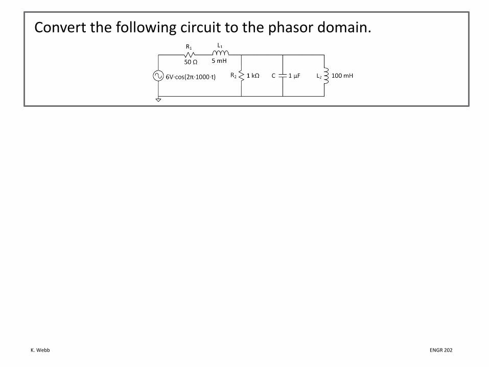
Convert the following circuit to the phasor domain.

K. Webb ENGR 202

K. Webb ENGR 202

The following current is applied to the capacitor. 𝑖𝑖 𝑡𝑡 = 100𝑚𝑚𝐴𝐴 ⋅ cos 2𝜋𝜋 ⋅ 50𝑘𝑘𝐻𝐻𝐻𝐻 ⋅ 𝑡𝑡

Find the voltage across the capacitor, 𝑣𝑣 𝑡𝑡 .

K. Webb ENGR 202

K. Webb ENGR 202

The following voltage is applied to the inductor. 𝑣𝑣 𝑡𝑡 = 4𝑉𝑉 ⋅ cos 2𝜋𝜋 ⋅ 800𝐻𝐻𝐻𝐻 ⋅ 𝑡𝑡

Find the current through the inductor, 𝑖𝑖 𝑡𝑡 .

K. Webb ENGR 202

A test voltage is applied to the input of an electrical network.

𝑣𝑣 𝑡𝑡 = 1𝑉𝑉 ⋅ sin 2𝜋𝜋 ⋅ 5𝑘𝑘𝐻𝐻𝐻𝐻 ⋅ 𝑡𝑡The input current is measured.

𝑖𝑖 𝑡𝑡 = 268𝑚𝑚𝐴𝐴 ⋅ sin 2𝜋𝜋 ⋅ 5𝑘𝑘𝐻𝐻𝐻𝐻 ⋅ 𝑡𝑡 − 46°What is the circuit’s input impedance, 𝑍𝑍𝑚𝑚𝑚𝑚?

K. Webb ENGR 202

Impedance of Arbitrary Networks49

K. Webb ENGR 202

50

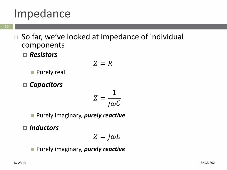
Impedance

So far, we’ve looked at impedance of individual components Resistors

𝑍𝑍 = 𝑅𝑅 Purely real

Capacitors

𝑍𝑍 =1𝑗𝑗𝜔𝜔𝐶𝐶

Purely imaginary, purely reactive

Inductors𝑍𝑍 = 𝑗𝑗𝜔𝜔𝐿𝐿

Purely imaginary, purely reactive

K. Webb ENGR 202

51

Impedance

Also want to be able to characterize the impedance of electrical networks Multiple components Some resistive, some reactive

In general, impedance is a complex value

𝑍𝑍 = 𝑅𝑅 + 𝑗𝑗𝑗𝑗where

𝑅𝑅 is resistance 𝑗𝑗 is reactance

So, in ENGR 201 we dealt with impedance all along Resistance is an impedance whose reactance (imaginary part) is

zero A purely real impedance

K. Webb ENGR 202

52

Reactance

For capacitor and inductors, impedance is purely reactive Resistive part is zero

𝑍𝑍𝑐𝑐 = 𝑗𝑗𝑗𝑗𝑐𝑐 and 𝑍𝑍𝐿𝐿 = 𝑗𝑗𝑗𝑗𝐿𝐿

where 𝑗𝑗𝑐𝑐 is capacitive reactance

𝑗𝑗𝑐𝑐 = − 1𝜔𝜔𝜔𝜔

and 𝑗𝑗𝐿𝐿 is inductive reactance

𝑗𝑗𝐿𝐿 = 𝜔𝜔𝐿𝐿

Note that reactance is a real quantity It is the imaginary part of impedance

Units of reactance: ohms (Ω)

K. Webb ENGR 202

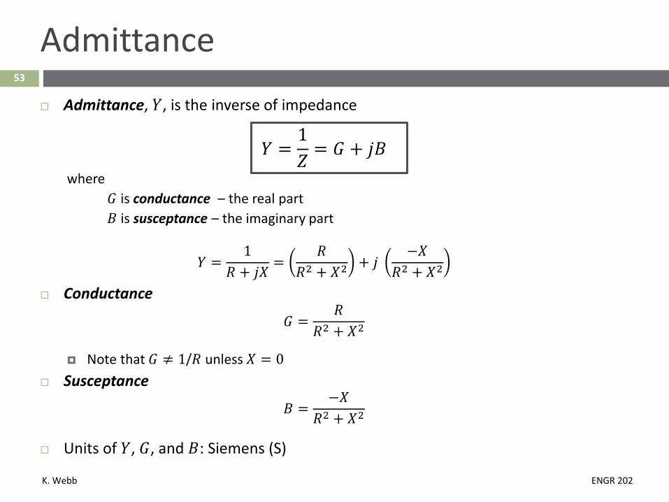
53

Admittance Admittance, 𝑌𝑌, is the inverse of impedance

𝑌𝑌 =1𝑍𝑍

= 𝐺𝐺 + 𝑗𝑗𝑗𝑗where

𝐺𝐺 is conductance – the real part𝑗𝑗 is susceptance – the imaginary part

𝑌𝑌 =1

𝑅𝑅 + 𝑗𝑗𝑗𝑗=

𝑅𝑅𝑅𝑅2 + 𝑗𝑗2

+ 𝑗𝑗−𝑗𝑗

𝑅𝑅2 + 𝑗𝑗2

Conductance

𝐺𝐺 =𝑅𝑅

𝑅𝑅2 + 𝑗𝑗2

Note that 𝐺𝐺 ≠ 1/𝑅𝑅 unless 𝑗𝑗 = 0 Susceptance

𝑗𝑗 =−𝑗𝑗

𝑅𝑅2 + 𝑗𝑗2

Units of 𝑌𝑌, 𝐺𝐺, and 𝑗𝑗: Siemens (S)

K. Webb ENGR 202

54

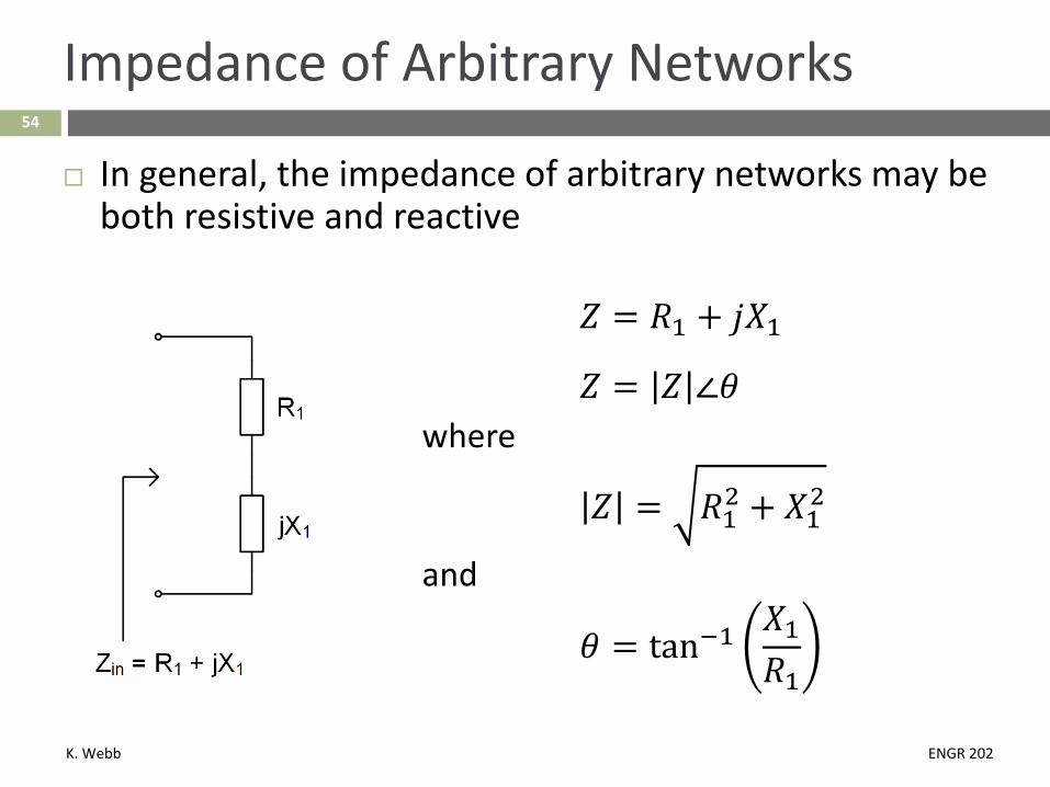
Impedance of Arbitrary Networks

In general, the impedance of arbitrary networks may be both resistive and reactive

𝑍𝑍 = 𝑅𝑅1 + 𝑗𝑗𝑗𝑗1

𝑍𝑍 = 𝑍𝑍 𝑟𝜃𝜃where

𝑍𝑍 = 𝑅𝑅12 + 𝑗𝑗12

and

𝜃𝜃 = tan−1𝑗𝑗1𝑅𝑅1

K. Webb ENGR 202

55

Impedances in Series

Impedances in series add

𝑍𝑍𝑒𝑒𝑒𝑒 = 𝑍𝑍1 + 𝑍𝑍2

𝑍𝑍𝑒𝑒𝑒𝑒 = 𝑅𝑅1 + 𝑅𝑅2 + 𝑗𝑗 𝑗𝑗1 + 𝑗𝑗2

K. Webb ENGR 202

56

Impedances in Parallel

Admittances in parallel add

𝑌𝑌𝑒𝑒𝑒𝑒 = 𝑌𝑌1 + 𝑌𝑌2

𝑍𝑍𝑒𝑒𝑒𝑒 =1𝑌𝑌𝑒𝑒𝑒𝑒

=1𝑍𝑍1

+1𝑍𝑍2

−1

𝑍𝑍𝑒𝑒𝑒𝑒 =𝑍𝑍1𝑍𝑍2𝑍𝑍1 + 𝑍𝑍2

K. Webb ENGR 202

Sinusoidal Steady-State Analysis57

K. Webb ENGR 202

58

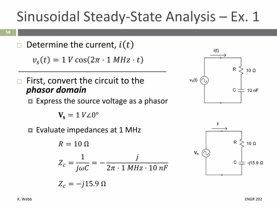
Sinusoidal Steady-State Analysis – Ex. 1

Determine the current, 𝑖𝑖 𝑡𝑡𝑣𝑣𝑠𝑠 𝑡𝑡 = 1 𝑉𝑉 cos 2𝜋𝜋 ⋅ 1 𝑀𝑀𝐻𝐻𝐻𝐻 ⋅ 𝑡𝑡

First, convert the circuit to the phasor domain Express the source voltage as a phasor

𝐕𝐕𝐬𝐬 = 1 𝑉𝑉𝑟0°

Evaluate impedances at 1 MHz

𝑅𝑅 = 10 Ω

𝑍𝑍𝑐𝑐 =1𝑗𝑗𝜔𝜔𝐶𝐶

= −𝑗𝑗

2𝜋𝜋 ⋅ 1 𝑀𝑀𝐻𝐻𝐻𝐻 ⋅ 10 𝑛𝑛𝑛𝑛

𝑍𝑍𝑐𝑐 = −𝑗𝑗15.9 Ω

K. Webb ENGR 202

59

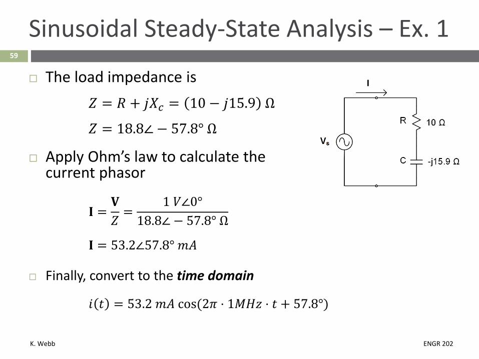
Sinusoidal Steady-State Analysis – Ex. 1

The load impedance is𝑍𝑍 = 𝑅𝑅 + 𝑗𝑗𝑗𝑗𝑐𝑐 = 10 − 𝑗𝑗15.9 Ω

𝑍𝑍 = 18.8𝑟 − 57.8° Ω

Apply Ohm’s law to calculate the current phasor

𝐈𝐈 =𝐕𝐕𝑍𝑍

=1 𝑉𝑉𝑟0°

18.8𝑟 − 57.8° Ω

𝐈𝐈 = 53.2𝑟57.8° 𝑚𝑚𝐴𝐴

Finally, convert to the time domain

𝑖𝑖 𝑡𝑡 = 53.2 𝑚𝑚𝐴𝐴 cos(2𝜋𝜋 ⋅ 1𝑀𝑀𝐻𝐻𝐻𝐻 ⋅ 𝑡𝑡 + 57.8°)

K. Webb ENGR 202

𝑣𝑣𝑠𝑠 𝑡𝑡 = 170 𝑉𝑉 sin 2𝜋𝜋 ⋅ 60𝐻𝐻𝐻𝐻 ⋅ 𝑡𝑡

60

Sinusoidal Steady-State Analysis – Ex. 2

Determine: The impedance, 𝑍𝑍𝑚𝑚𝑚𝑚, at 60 Hz Voltage across the load, 𝑣𝑣𝐿𝐿 𝑡𝑡 Current delivered to the load, 𝑖𝑖𝐿𝐿 𝑡𝑡

Consider the following circuit, modeling a source driving a load through a transmission line

K. Webb ENGR 202

61

Sinusoidal Steady-State Analysis – Ex. 2

First, convert to the phasor domain and evaluate impedances at 60 Hz

The line impedance is

𝑍𝑍𝑙𝑙𝑚𝑚𝑚𝑚𝑒𝑒 = 𝑅𝑅1 + 𝑗𝑗𝜔𝜔𝐿𝐿1 = 0.5 + 𝑗𝑗1.88 Ω

The load impedance is

𝑍𝑍𝑙𝑙𝑙𝑙𝑚𝑚𝑙𝑙 = 𝑅𝑅2 + 𝑗𝑗𝜔𝜔𝐿𝐿2 ||1𝑗𝑗𝜔𝜔𝐶𝐶 = 3 + 𝑗𝑗5.65 Ω || − 𝑗𝑗265 Ω

𝑍𝑍𝑙𝑙𝑙𝑙𝑚𝑚𝑙𝑙 =1

3 + 𝑗𝑗5.65 Ω +1

−𝑗𝑗265 Ω

−1

= 3.13 + 𝑗𝑗5.74 Ω

K. Webb ENGR 202

62

Sinusoidal Steady-State Analysis – Ex. 2

The impedance seen by the source is𝑍𝑍𝑚𝑚𝑚𝑚 = 𝑍𝑍𝑙𝑙𝑚𝑚𝑚𝑚𝑒𝑒 + 𝑍𝑍𝑙𝑙𝑙𝑙𝑚𝑚𝑙𝑙𝑍𝑍𝑚𝑚𝑚𝑚 = 0.5 + 𝑗𝑗1.88 Ω + 3.13 + 𝑗𝑗5.74 Ω

𝑍𝑍𝑚𝑚𝑚𝑚 = 3.63 + 𝑗𝑗7.62 Ω

In polar form:𝑍𝑍𝑚𝑚𝑚𝑚 = 8.44𝑟64.5° Ω

The impedance driven by the source looks resistive and inductive Resistive: non-zero resistance, 𝑟𝑍𝑍𝑚𝑚𝑚𝑚 ≠ ±90° Inductive: positive reactance, positive angle

K. Webb ENGR 202

63

Sinusoidal Steady-State Analysis – Ex. 2

𝐕𝐕𝐿𝐿 = 𝐕𝐕𝑆𝑆𝑍𝑍𝑙𝑙𝑙𝑙𝑚𝑚𝑙𝑙

𝑍𝑍𝑙𝑙𝑚𝑚𝑚𝑚𝑒𝑒 + 𝑍𝑍𝑙𝑙𝑙𝑙𝑚𝑚𝑙𝑙

𝐕𝐕𝐿𝐿 = 170𝑟0° 𝑉𝑉3.13 + 𝑗𝑗5.74 Ω3.63 + 𝑗𝑗7.62 Ω

𝐕𝐕𝐿𝐿 = 170𝑟0° 𝑉𝑉6.54𝑟61.4° Ω8.44𝑟64.5° Ω = 132𝑟 − 3.1° 𝑉𝑉

Converting to time-domain form

𝑣𝑣𝐿𝐿 𝑡𝑡 = 132 𝑉𝑉 sin 2𝜋𝜋 ⋅ 60𝐻𝐻𝐻𝐻 ⋅ 𝑡𝑡 − 3.1°

Apply voltage division to determine the voltage across the load

K. Webb ENGR 202

64

Sinusoidal Steady-State Analysis – Ex. 2

𝐈𝐈𝐿𝐿 =𝐕𝐕𝐿𝐿𝑍𝑍𝑙𝑙𝑙𝑙𝑚𝑚𝑙𝑙

𝐈𝐈𝐿𝐿 =132𝑟 − 3.1° 𝑉𝑉6.54𝑟61.4° Ω

𝐈𝐈𝐿𝐿 = 20.1𝑟 − 64.5° 𝐴𝐴

In time-domain form:𝑖𝑖𝐿𝐿 𝑡𝑡 = 20.1 𝐴𝐴 sin 2𝜋𝜋 ⋅ 60𝐻𝐻𝐻𝐻 ⋅ 𝑡𝑡 − 64.5°

Finally, calculate the current delivered to the load

K. Webb ENGR 202

Example Problems65

K. Webb ENGR 202

Determine the input impedance and an equivalent circuit model for the following network at 50 kHz.

K. Webb ENGR 202