153 Section Five: Cost-benefit analysis and priority setting 5.1 Methodology This cost-benefit analysis assesses the difference between two scenarios: ‘No change’ and ‘Actions implemented’ scenarios. The ‘No change’ scenario represents the prevailing situation at the beginning of the research period. It differs from a ‘do-nothing’ scenario because it takes into account salinity management strategies or actions that are in place. This is a regional level analysis that estimates the total benefits and costs of implementation of the recommendations for the entire Port Phillip and Western Port region. The analysis estimates a Net Present Value (NPV), Cost-Benefit Ratio (BCR) and Internal Rate of Return (IRR) of implementing the recommended salinity management programs. The analysis is based upon the recommended implementation targets in each of the 12 Salinity Management Zones described in Section 4. Data Collection Data sets used in this analysis were collected from a number of sources including the National Land and Water Resources Audit (NLWRA), the Geographical Information System Group of DPI, and other data sets held by DPI, DSE, ABS and ABARE. The major data sets used in this analysis were: • Regional Groundwater Flow Systems and land use data; • Roads, housing and other infrastructure within the Salinity Management Zones; • Regional gross margin, price and productivity figures (by enterprise) (sourced from ABS, DPI, and ABARE; • Area under shallow water tables in Salinity Management Zones; • Regional averages of production and prices - (pasture, cropping & horticulture); • Area with shallow watertables <2m, 2-5m, 5-10m, 10-15m, 15-20m; • Melbourne 2030 growth corridors and green wedges; • Distribution of production losses across different land uses; • Relationship between water table depth and production losses; and • Relationship between salinity and infrastructure maintenance costs. Assumptions The impacts of salinity were estimated and analysed against the estimated project costs. They included: • Agricultural production losses; • Extra costs to roads and urban infrastructure; • Environmental damages due to salinity; and • Any other quantifiable production benefits. The direct and quantifiable losses due to the salinity problem in the region, especially in the 12 identified Salinity Management Zones, were calculated for current and future conditions based on predictions of rising water tables.
Transcript
153
Section Five: Cost-benefit analysis and priority setting 5.1 Methodology This cost-benefit analysis assesses the difference between two scenarios: ‘No change’ and ‘Actions implemented’ scenarios. The ‘No change’ scenario represents the prevailing situation at the beginning of the research period. It differs from a ‘do-nothing’ scenario because it takes into account salinity management strategies or actions that are in place. This is a regional level analysis that estimates the total benefits and costs of implementation of the recommendations for the entire Port Phillip and Western Port region. The analysis estimates a Net Present Value (NPV), Cost-Benefit Ratio (BCR) and Internal Rate of Return (IRR) of implementing the recommended salinity management programs. The analysis is based upon the recommended implementation targets in each of the 12 Salinity Management Zones described in Section 4.
Data Collection Data sets used in this analysis were collected from a number of sources including the National Land and Water Resources Audit (NLWRA), the Geographical Information System Group of DPI, and other data sets held by DPI, DSE, ABS and ABARE. The major data sets used in this analysis were:
• Regional Groundwater Flow Systems and land use data; • Roads, housing and other infrastructure within the Salinity Management Zones; • Regional gross margin, price and productivity figures (by enterprise) (sourced from ABS, DPI, and
ABARE; • Area under shallow water tables in Salinity Management Zones; • Regional averages of production and prices - (pasture, cropping & horticulture); • Area with shallow watertables <2m, 2-5m, 5-10m, 10-15m, 15-20m; • Melbourne 2030 growth corridors and green wedges; • Distribution of production losses across different land uses; • Relationship between water table depth and production losses; and • Relationship between salinity and infrastructure maintenance costs.
Assumptions The impacts of salinity were estimated and analysed against the estimated project costs. They included:
• Agricultural production losses; • Extra costs to roads and urban infrastructure; • Environmental damages due to salinity; and • Any other quantifiable production benefits.
The direct and quantifiable losses due to the salinity problem in the region, especially in the 12 identified Salinity Management Zones, were calculated for current and future conditions based on predictions of rising water tables.
154
The ‘No change’ and ‘Actions implemented’ scenarios were compared to calculate the actual benefits or disadvantages of implementing actions. Estimations were heavily based on the findings of the National Land and Water Resources Audit: Theme 2 – Dryland Salinity (NLWR 2000), and this report’s analysis of Groundwater Flow Systems. Estimations of agricultural benefits were based on the potential value of lost agricultural production due to salinity (such losses would be partly ameliorated through the implementation of the recommended actions), and productivity gains due to the improved conditions for major agricultural industries in the Salinity Management Zones (i.e. improvements in the quality of farming land are likely to result in establishment of some higher value enterprises compared with the current situation). It is unlikely that the entire area within each Salinity Management Zone would be uniformly affected by shallow water tables and salinity. Agricultural losses could be grossly overestimated if it were assumed that the entire area was affected that way. Therefore, the following conservative assumptions were made when estimating agricultural and infrastructure losses caused by salinity: • Plant growth and agricultural production is assumed to be affected in only 50% of the area with a depth to water
table of less than two metres. Agricultural production within affected areas is assumed to be reduced, causing a 75% reduction in gross margins; and
Estimates of additional road costs due to salinity were based on local expert opinions and findings of the Audit report (NLWR 2000). It is assumed that about 25% of existing roads in all Salinity Management Zones are categorised as being ‘very slightly’ impacted by salinity in 2006. If there is no specific plan to manage salinity, then by 2016 that is estimated to increase to a ‘slight’ impact and by 2026, to a ‘moderate’ impact.
Data Analysis The potential benefits of implementing the recommended salinity management actions include: • Minimised financial losses to agricultural enterprises; • Generating agricultural productivity improvements and land use changes; • Reducing the repair and maintenance costs of roads and railways; • Reducing costs for buildings and other infrastructure developments; and • Other environmental and social benefits. Agricultural impacts were estimated using gross margins based on long-term farm gate prices of major agricultural commodities produced in the region. The impacts of salinity on infrastructure assets were estimated as were the additional costs to roads, railways, building and industrial assets and underground services (water, stormwater, sewerage, telecommunications, gas, electricity). Wherever possible the impacts of salinity and high watertables for parks and recreational venues and environmental and other social amenities were quantified and taken into consideration. However most of the environmental and social benefits from implementation of recommended actions from this report are difficult to quantify in monetary terms. Where possible those benefits are quantified in non-monetary terms, such as the area of wetlands protected and the number of native species protected. They are then considered in a priority setting process. The analysis undertakes an economic evaluation in terms of Net Present Value (NPV1), Internal Rate of Return (IRR2) and Cost-Benefit Ratio (BCR3). The higher the NPV and BCR, the more economically viable is the project.
1 Net present value (NPV) is the difference between the discounted values at a required discount rate of the future benefits
and costs associated with the project. The higher the NPV the more economically viable is the project because the project is earning at that rate plus some more. If the NPV is negative, the project is not economically viable.
155
A standard discounted cash flow analysis was used to calculate the Net Present Value, Cost-Benefit Ratio and Internal Rate of Return of the recommended actions. As required by Victorian State Government guidelines, 4% and 8% discount rates were applied. The 4% discount rate refers to the return Victorian State Government expects from its investment in natural resource management activities, while the 8% discount rate reflects the assumed financial return private landholders could expect from their investment. The lifespan of all project activities and impacts was assumed to be 30 years. To calculate the actual benefits and costs associated with salinity management, it is necessary to deal with net returns rather than gross returns for a region. Gross margins are the most appropriate measure of net returns from agricultural production. Limitations of the Study The analysis was limited by the availability of data and resources. Except for the agricultural production benefits and costs, other major possible benefits and costs components were mostly dependent on expert opinions, research findings and experiences from other regions and States. That may have resulted in over or under valuing certain costs and benefits. However the findings of the analysis gave an indication of the overall economic worthiness of implementing the recommended actions and a good indication of where data and information were lacking. The social benefits and costs such as lifestyle impacts, internal migration of communities due to salinity, and estimates of how well the community is working together to overcome the problem were not covered by this study. The following possible benefits were not quantitatively measured:
• Enhanced amenity; • Water quality benefits; • Improved safety on roads; • Improved quality of life ; • Reduced health risks to both humans and animals; • Increased property values due to improved drainage; and • Reduced water logging.
Additional costs to farmers, such as the value of equipment and materials they may need to buy in order to implement some activities, were not measured.
5.2 Economic impacts of salinity on the agriculture sector Assessment of the economic losses in agricultural production due to salinisation in Port Phillip and Western Port region involved the following steps:
• Estimating the total gross margin of agricultural production in the region; • Specifying the gross margin loss function, based on a relationship between the area under high watertables
and loss in production; and
2 Internal rate of return (IRR) is the break-even discount rate. It is the discount rate at which the present value of the
benefits from a project equals the present value of the costs of the project. The higher the IRR, the more economically attractive is the project.
3 Benefit-cost ratio (BCR) is the ratio of the present value of project benefits to the present value of project costs. The higher the BCR, the more economically viable is the project because it is earning more than the required rate of return. A BCR of 1.04 means that for every dollar spent on the project, the benefits generated were valued at $1.04.
156
• Applying the loss function by using the projected changes in the area of high watertables and calculating changes in total gross margins.
The agriculture industry in the Port Phillip and Western Port region covers approximately 240,000 hectares generating gross margins of about $69 million (Table 78). Pasture-based industries contribute 65% of the gross margins, 28% from horticulture and the balance from cereal, legume and oilseed crops. Table 78: Estimated total annual gross margins of agriculture industries in the region
Total 240,626 $68.67 Notes: Based on ABS 2004, DNRE GM publications and ABARE commodity reports. 2006 $ values. The area affected by salinisation in 2006 is estimated to be about 1.4% (3425ha) of the agricultural area in the region (Table 79). By 2016 it is estimated that the affected area will double, increasing to 12,000 hectares in 2026 in the absence of a plan to manage the problem. The value of these losses in 2006 is $900,000 increasing to $3 million by 2026 (Table 80). Table 79: Estimated area (ha) of agriculture affected by salinity in the region
Land use 2006 2016 2026 Pasture (dairy) 587 1,178 2,008 Pasture (beef & sheep mixed ) 2,348 4,711 8,023
Cereal, legume & oilseed crops 484 938 1,500
Fruits 3 28 78
Vegetables 3 41 116 Total area affected (ha) 3,425 6,897 11,736
157
Table 80: Estimated gross margin foregone in the region due to salinity
Land use 2006 2016 2026 Pasture (dairy) $527,420 $1,058,433 $1,804,188
Total gross margin foregone $855,103 $1,752,410 $3,025,934 Notes: These calculations are based on Audit Report’s (NLWR 2000) predicted 75% of GM losses due to salinity. 2006 $ values.
5.3 Economic impacts of salinity on the infrastructure sector Urban salinity affects the built environment in many ways, due to the chemical and physical impacts of salt on concrete, bricks and metal. This can result in considerable damage to buildings, roads and railways. All such impacts of salinity on public infrastructure contribute to high community costs. In the Murray Darling Basin it is estimated that approximately 60% of non-agricultural costs due to salinity are from road damage (Murray Darling Basin Salinity Audit 1999). Much of the cost of urban salinity is borne by local authorities in the form of increased infrastructure repair costs, asset maintenance and replacement costs, and decreased useability of assets. While it is not possible to directly transfer cost figures from one area to another, it is instructive to consider figures from Wagga Wagga City Council which indicate the potential magnitude of costs of salinity in an urban environment (Table 81). These figures indicate the annual recurring costs assuming that 1/9th of the urban area within Wagga Wagga City Council was affected by salinity, and that nothing is done to manage the salinity problem. Table 81: Estimated annual cost of salinity in an urban area
Infrastructure Annual Cost Roads $226,000
Footpaths $4,400
Parks $103,400
Houses $72,500
Industrial $6,000
Note: 1995 $ values (Christiansen, 1995)
158
Roads and railway infrastructure There are about 17,000 km of roads in the Port Phillip and Western Port region. Predictions using the findings of the Audit Report (NLWR 2000) estimate a very slight impact on the road and railways network in 2006, slight impact in 2016 and a moderate impact in 2026. The estimated length of roads and railways at risk from salinisation and waterlogging is about 1,200 km in 2006, 2,800 km in 2016 and 4,600 km in 2026 (Table 82). Table 82: Potential impact of salinity on major roads (affected km) in the region
Main road - sealed 1,157 81.0 196.7 324.0 Main road - unsealed 332 23.2 56.4 93.0
Other road - sealed 7,632 534.2 1297.4 2,137.0
Other road - unsealed 6,414 449.0 1090.4 1,795.9 Total road network 16,543 1,158.0 2,812.3 4,632.1 Railways 89 1.3 6.8 20.7
Wilson (2000) estimated that the additional repair and maintenance cost due to salinisation ranges from $101 to $42,000 per km depending on the severity of the impact and road classification (Table 83). Table 83: Estimated additional repair and maintenance cost due to salinity by road class and severity of damage
Road Class Very Slight
Impact ($/km/yr)
Slight Impact ($/Km/Yr)
Moderate Impact ($/Km/Yr)
Severe Impact ($/Km/yr)
National and State Highway $1,077 $1,615 $4,846 $41,975 Main Sealed Road $269 $606 $2,154 $23,319
Minor Sealed Road $135 $404 $942 $1,615
Unsealed Road $101 $269 $673 $1,077
Notes: CPI adjusted values - General Construction. 2006 $ values. (Wilson 2000) Using Tables 82 and 83, the estimated cost of additional repair and maintenance is $220,000 in 2006, $1.3 million in 2016 and $5.6 million in 2026 (Table 84).
159
Table 84: Estimated total annual extra cost for repair & maintenance of roads due to salinity
Infrastructure
Very Slight Impacts
2006
$/yr
Slight Impacts
2016
$/yr
Moderate Impacts
2026
$/yr
Free way - sealed $34,572 $125,809 $621,257
High way - sealed $41,465 $151,003 $746,284
Main road - sealed $21,789 $119,261 $698,111
Main road - unsealed $2,343 $15,172 $62,589
Other road - sealed $72,117 $524,150 $2,013,054
Other road - unsealed $45,349 $293,318 $1,208,641
Total road network $217,634 $1,228,711 $5,349,936
Railways $3,150 $66,817 $289,759
Total extra cost $220,784 $1,295,527 $5,639,695
Notes: These estimates take into account only the existing road & railway network in Salinity Management Zones. 2006 $ values.
Building and other infrastructure assets Estimates of watertable depths used in NLWRA reports on dryland salinity have indicated that a number of townships and parts of townships such as Romsey, Hastings and Ballan are in slight risk zones (groundwater 5 to 10 m). Projections by SKM and the Audit Report (NLWR 2000) indicate that those watertables are likely to rise further over the next 50 years. A study conducted in Wagga Wagga and Western Sydney indicated that new residential developments in high watertable urban areas could incur additional costs due to salinity and waterlogging. The cost ranges from $632 to $8,400 per building unit, depending on the severity of the salinity impact (Table 85). Table 85: Estimated additional expenditure for new residential development
Very Slight Impact Slight Impact Moderate impact Severe impact
Average value of range $1,159 $2,283 $4,110 $6,730
Notes: • Calculations based on information from: Impact of urban salinity in Wagga Wagga 1998, DLWC NSW,
Christensen 1995 and Planning Division of Casey City Council. • ABARE, costs of dryland salinity to local Government, consultancy for MDBC, Canberra 1995. • The 1998 values were adjusted by CPI - General Construction. • 2006 $ values.
160
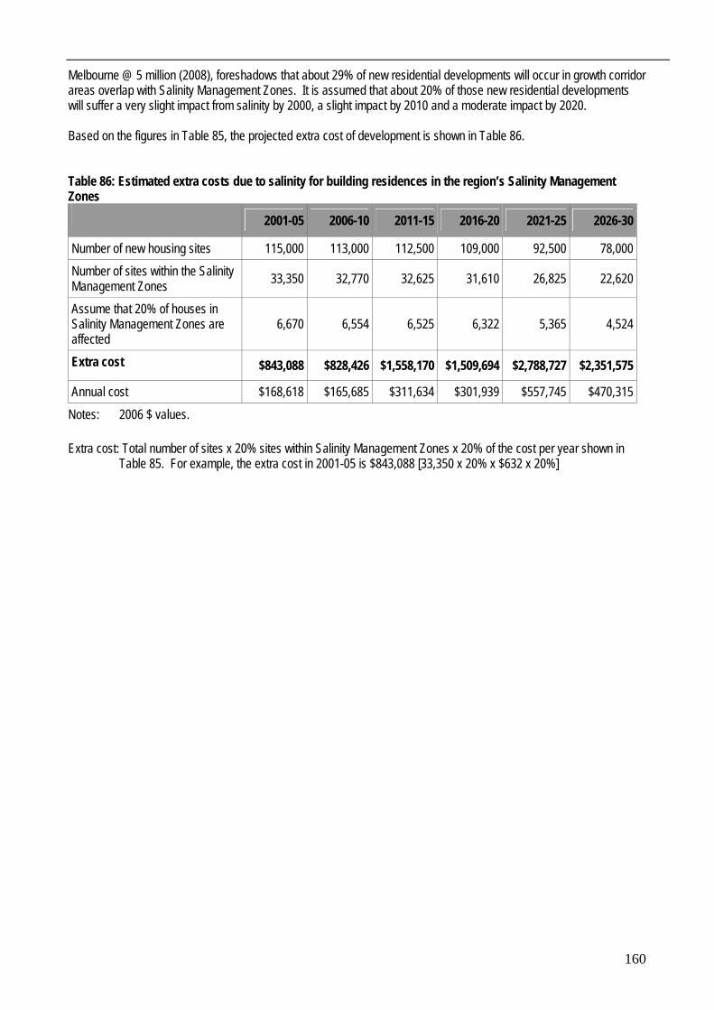
Melbourne @ 5 million (2008), foreshadows that about 29% of new residential developments will occur in growth corridor areas overlap with Salinity Management Zones. It is assumed that about 20% of those new residential developments will suffer a very slight impact from salinity by 2000, a slight impact by 2010 and a moderate impact by 2020. Based on the figures in Table 85, the projected extra cost of development is shown in Table 86. Table 86: Estimated extra costs due to salinity for building residences in the region’s Salinity Management Zones
2001-05 2006-10 2011-15 2016-20 2021-25 2026-30
Number of new housing sites 115,000 113,000 112,500 109,000 92,500 78,000 Number of sites within the Salinity Management Zones 33,350 32,770 32,625 31,610 26,825 22,620
Assume that 20% of houses in Salinity Management Zones are affected
6,670 6,554 6,525 6,322 5,365 4,524
Extra cost $843,088 $828,426 $1,558,170 $1,509,694 $2,788,727 $2,351,575
Annual cost $168,618 $165,685 $311,634 $301,939 $557,745 $470,315 Notes: 2006 $ values. Extra cost: Total number of sites x 20% sites within Salinity Management Zones x 20% of the cost per year shown in
Table 85. For example, the extra cost in 2001-05 is $843,088 [33,350 x 20% x $632 x 20%]
161
Underground services (water, stormwater, sewerage, telecommunications, gas, electricity) High watertables and salinity can affect the operating life and maintenance cost of most underground infrastructure services. Saline groundwater and high watertables can be corrosive towards underground pipes, reducing the life of these assets. Detailed studies on the impacts of salinity on underground services in the region have not been undertaken, however information gathered from other areas can be used to develop relevant estimates. Gippsland Water estimated the impact of high watertables on sewerage systems in the urban areas of Sale in 1998. They found that the need to operate additional pumps to pump groundwater infiltrating into sewerage mains adds considerably to the operating costs of sewerage systems in Sale and other townships in the area. With respect to these additional pumping costs, it is estimated that the average wastewater pumping cost was $10 per property in moderate risk zones and $4 per property in low risk zones. Wilson (2001) estimated that in the Goulburn Broken region the cost of the reduced lifespan of underground infrastructure services due to salinity are in the range of $48 – $160 per household in the urban areas. Analysis of feedback from infrastructure related companies and council officials in the region indicated that salinity and high watertables add an extra $26.204 to the cost of supplying underground services to new building sites in the region per site. Accordingly the estimated total extra cost is shown in Table 87. Table 87: Estimated extra costs for underground services in Salinity Management Zones due to salinity
Note: 2006 $ values The estimated additional cost of maintenance and development of infrastructure assets in the region due to salinity and waterlogging is shown in Table 88. Table 88: Estimated extra costs of maintenance and development of infrastructure in the SMZ’s
Infrastructure Year 10 Year 20 Year 30
Roads $1,188,050 $5,205,280 $5,639,695
Housing $303,878 $487,801 $470,315
Underground services $166,699 $122,935 $118,529 Total $1,658,627 $5,816,017 $6,228,539
Note: 2006 $ values
4 The extra cost was $24.-8 in 2004$ and was adjusted by CPI-General Construction to 2006$
162
5.4 Economic Analysis Generally, projects with a cost-benefit ratio of at least 1:1 and a positive net present value at 4 % over 30 years are considered economically attractive.
Benefits – Agriculture and Infrastructure Sectors The benefits of implementing recommended actions to the agriculture sector are mainly from losses avoided. However some activities are associated with dual benefits. For example, conversion from annual pasture to perennial pasture or lucerne will reduce the impact of salinity and at the same time increase gross production by introducing higher value crops (see Tables 89 and 90). It is also predicted that the productivity of existing enterprises will increase as greater confidence in the future of agriculture will result in a greater willingness for landholders to invest in higher value farming activities. The estimated value of agricultural losses due to salinity and waterlogging is about $900,000 in 2006 and $3 million in 2026. With the implementation of recommended actions, up to 50% of these losses can be avoided. Activities to reduce the effects of salinity, whilst beneficial overall, also incur some agricultural disadvantages as some agricultural land is turned over to permanent tree plantations for recharge control. The value of agricultural benefits (after subtracting the dis-benefits) ranges from $1 million in year 10 to $2.5 million in year 30 following implementation of recommended actions. Table 89: Estimated value of agricultural benefits in Year 10, Year 20 and Year 30
Benefits Year 10 Year 20 Year 30
Agricultural losses avoided through groundwater pumping, drainage, tree planting etc.
$822,813 $1,440,602 $2,246,773
Land use change (salt tolerant pasture, perennial pasture, lucerne) $264,306 $264,306 $264,306
Extra gross margin due to increase productivity $169,336 $271,363 $281,400
Lost production due to land retirement (for tree planting and revegetation) -$241,920 -$241,920 -$241,920
Net agricultural benefits $1,014,535 $1,734,351 $2,550,559 Note: 2006 $ values Table 90: Estimated annual extra gross margins of existing land use due to increased productivity within the Salinity Management Zones
Total $169,336 $271,363 $281,400 Notes: Pasture dairy includes additional dairy farm land. 2006 $ values.
163
The implementation of the recommended actions is predicted to reduce about 40% of additional cost of road and railway maintenance, housing development and other infrastructure assets. The value of these benefits in years 10, 20 and 30 following implementation of the recommended actions is shown in Table 91. Table 91: Estimated value infrastructure benefits in Year 10, Year 20 and Year 30
Total benefits $663,451 $2,326,407 $2,491,416 Note: 2006 $ values
Estimated costs of implementing actions Implementation of the recommended actions will cost about $17.2 million over five years. This report proposes five programs and each are individually costed (Tables 92 and 93) within each Salinity Management Zone (see Section 4). Table 92: Estimated cost of implementing the recommended programs
Recommended Programs 5-year cost % of total cost
Agriculture & Drainage $4.28 24.9%
Environment management $6.10 35.5%
Salinity Monitoring and R&D $3.22 18.7% Education $1.62 9.4%
Program support $1.98 11.5%
Total cost $17.20 100% Note: 2006 $ values Table 93: Estimated annual cost of implementing the recommended programs
Recommended Programs Year 1 Year 2 Year 3 Year 4 Year 5
Program support $396,000 $396,000 $396,000 $396,000 $396,000
Total cost $2,215,822 $4,393,999 $3,641,423 $3,641,423 $3,308,431
% of total cost 13% 26% 21% 21% 19%
Note: 2006 $ values
164
The estimated operation and maintenance cost of drains and groundwater pumps were not included in Tables 92 and 93. These costs however were included in the cash flow analysis. The downstream cost of the salinity was not calculated due to lack of data on salt loads in the streams in the region.
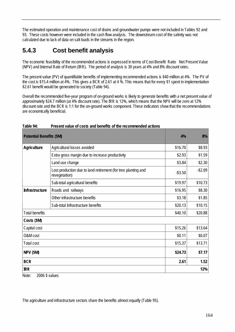
5.4.3 Cost benefit analysis The economic feasibility of the recommended actions is expressed in terms of Cost-Benefit Ratio Net Present Value (NPV) and Internal Rate of Return (IRR). The period of analysis is 30 years at 4% and 8% discount rates. The present value (PV) of quantifiable benefits of implementing recommended actions is $40 million at 4%. The PV of the cost is $15.4 million at 4%. This gives a BCR of 2.61 at 4 %. This means that for every $1 spent in implementation $2.61 benefit would be generated to society (Table 94). Overall the recommended five-year program of on-ground works is likely to generate benefits with a net present value of approximately $24.7 million (at 4% discount rate). The IRR is 12%, which means that the NPV will be zero at 12% discount rate and the BCR is 1:1 for the on-ground works component. These indicators show that the recommendations are economically beneficial. Table 94: Present value of costs and benefits of the recommended actions
Potential Benefits ($M) 4% 8%
Agricultural losses avoided $16.70 $8.93 Extra gross margin due to increase productivity $2.93 $1.59
Land use change $3.84 $2.30
Lost production due to land retirement (for tree planting and revegetation) -$3.50 -$2.09
Agriculture
Sub-total agricultural benefits $19.97 $10.73 Roads and railways $16.95 $8.30
Other infrastructure benefits $3.18 $1.85
Infrastructure
Sub-total Infrastructure benefits $20.13 $10.15
Total benefits $40.10 $20.88 Costs ($M) Capital cost $15.26 $13.64
O&M cost $0.11 $0.07
Total cost $15.37 $13.71
NPV ($M) $24.73 $7.17
BCR 2.61 1.52 IRR 12%
Note: 2006 $ values The agriculture and infrastructure sectors share the benefits almost equally (Table 95).
165
Table 95: Estimated percentage contribution to the benefits of recommended actions
Benefits % of total
Agricultural losses avoided 41.6%
Extra gross margin due to increase productivity 7.3% Land use change 9.6%
Lost production due to land retirement (for tree planting and revegetation) -8.7%
Agriculture
Sub-total agricultural benefits 49.8% Roads and railways 42.3% Other infrastructure benefits 7.9%
Infrastructure
Sub-total Infrastructure benefits 50.2% Total benefits 100%
5.4.4 Environmental and social benefits The economic feasibility of the recommended actions is expected to improve further if the benefits from environmental and social outcomes were included in the analysis. Estimates in the Shepparton Irrigation Region show that protection of environmental features has a significant financial value (Montecillo, 2006): • Protecting threatened or endangered species - $400,000 per species (2005$) per year for 20 years; • Protecting or restoring bushland - $45 per hectare per year for 20 years (2005$); and • Protecting or restoring wetlands - $580 per hectare per year (2005$, annualised at 4% for 30 years). The expected economic benefits from the implementation of the recommended actions at 8% discount rate are still attractive with a BCR of 2.61 and NPV of $24.7 million. However, it is important to note that unquantified environmental and social benefits remain a significant and important factor. The Port Phillip and Western Port region is one of the most biologically diverse in Victoria. Located at the boundary of four of Australia’s major bioregions and the junction of eight state bioregions it supports an extraordinary diversity of native plant and animal communities and environmentally valuable land and water resources. Recent studies conducted as part of the NLWRA Audit Report (NLWRA 2000) assessed the potential impacts of shallow watertables and dryland salinity on the natural environment of the State, including the Port Phillip and Western Port region. According to their findings, under the worst case scenario this region will have the greatest number of recorded Victorian Rare or Threatened (VROT) classified fauna in the areas threatened by shallow water tables (70 fauna and 48 flora species). Although it is stated that high watertables and salinity would threaten wetland health and environment quality, there has been no quantitative assessment of the extent to which such impacts might be realised in the region. Most of the environmental and social outcomes provided by improved salinity management (such as improved community health and well being, improved biodiversity etc.) are not traded in commercial markets and the values of those outcomes are difficult to estimate. Therefore such benefits are presented descriptively in this analysis (see Table 96).
166
Table 96: Likely environmental and social benefits of the recommended actions
Category Benefits resulting from the implementation of the recommended actions
Environmental Increase in terrestrial and aquatic biodiversity Improved environmental quality Protection of threatened ecological vegetation classes
Protection of rivers, wetlands and floodplain areas Protection of remnant vegetation Protection of fauna food sources and habitat Protection of natural resource assets Meeting international JAMBA / CAMBA / RAMSAR obligations Social Protection of recreational opportunities such as fishing, bushwalking and bird watching Protection of landscape aesthetics Protection of cultural heritage sites Improved community health and well-being Contributing factor to farm viability and rural life style: • Sporting and cultural networks
• Viability of community services
• Enhancement of social & cultural networks
Reduced need for off farm work leaving the rural communities Salinity management in the region will contribute to environmental protection in the region and hence supports: • 1,860 native flora species (vascular plants) and 616 native animals (vertebrate fauna); • 128 rare or threatened fauna species; of which 24 are listed under the Commonwealth EBPC Act (1999) and 61
are listed under the Victorian Flora and Fauna Guarantee Act (1988); • 302 rare or threatened flora species of which 25 are listed under the Commonwealth EBPC Act (1999) and 34
are listed under the Victorian Flora and Fauna Guarantee Act (1988); • 34 plants, 61 animals and 7 communities that are listed under the Flora and Fauna Guarantee Act 1988; • three sites listed under the Ramsar International Treaty on Wetlands; (Port Phillip Bay (Western Shoreline) and
Bellarine Peninsula, Edithvale-Seaford Wetlands and Western Port); and • 100 of Victoria’s 425 Ecological Vegetation Classes. 5.4.5 Conclusion The economic analysis indicates that the implementation program that this report proposes is a cost-effective method of protecting and enhancing the region’s agriculture, infrastructure, environmental and social values. It also shows that salinity management in the region would enhance the protection of regional infrastructure assets and improve agricultural productivity or protect the quality of agricultural areas for alternative future uses. It indicates that salinity management in the region can generate sufficient benefits to cover the cost of required management actions. The recommended actions are strongly economic but the foreshadowed benefits depend upon the timely implementation of both its agriculture and infrastructure programs.
167
5.4.6 Sensitivity Analysis Key variables used in the analysis were tested to determine the sensitivity of the economic indicators (BCR, NPV and IRR). Table 97 shows that the recommended actions will be economic under a range of scenarios. The exception is when the benefits are reduced to 60% and an 8% discount rate is applied. Table 97: Results of sensitivity analysis
Cost increase by 20% $21.64 $4.43 2.17 1.27 10% Cost increase by 40% $18.56 $1.69 1.86 1.09 9%
Note: 2006 $ values
5.5 Resource Allocation and Cost Sharing Salinity management is a challenge for rural and regional communities, industry and the government. Maintaining and enhancing a partnership approach is very important to successful salinity management. Implementation of the actions recommended in this report would require joint action among the community, industry and government as it produces benefits to both private individuals and the broader community. The process of priority setting in Salinity Management Zones took account of the responsiveness of groundwater flow systems, existing salinity and rising watertables, and the economic, environmental and social benefits associated with salinity management options. Details of public investments in key work components and cost sharing would need to be developed to reflect the outcomes of activities in accordance with Government Cost Sharing Guidelines. The Australian and Victorian Governments could contribute a share towards the cost of actions that generate wider community benefits. Local government, and service providers such as transport and power providers could contribute towards actions that protect their assets or generate other benefits to their constituents. Individuals and private businesses could contribute when they are the beneficiaries of action.
168
5.5.1 Program Costs and Benefits by Salinity Management Zones Table 98 is a summary of costs by recommended Program and by Salinity Management Zone in 2006 dollars. Table 98: Summary of the estimated cost of implementing actions over the first five years
12 Irrigation Areas $269,502 $0 $407,616 $139,392 $165,000 $981,510
TOTAL $4,280,514 $6,101,190 $3,217,369 $1,622,016 $1,980,000 $17,201,089 Notes: Excludes annual operation and maintenance of surface drains and groundwater pumps.
2006 $ values.
169
5.5.2 Cost Sharing An example of a cost share split for the implementation of the recommended actions is presented in Table 99, based on the projected distribution of projected benefits across major beneficiaries. Table 100 presents the annual cost share by major beneficiaries at 2006$ nominal value excluding the annual operation and maintenance of surface drains and groundwater pumps. Table 101 is based on the present value (2006 $ values) of all costs including implementation or capital cost, and operation and maintenance of drains and pumps. Table 99: Example of a cost share by major beneficiaries over five years
Yr 1 Yr 2 Yr 3 Yr 4 Yr 5 TOTAL ($M) % of total
State & Federal Governments $598,272 $1,186,380 $983,184 $983,184 $893,276 $4.64 27%
Local Governments $398,848 $790,920 $655,456 $655,456 $595,518 $3.10 18%
Ag Industries $155,108 $307,580 $254,900 $254,900 $231,590 $1.20 7%
Water Authorities $443,164 $878,800 $728,285 $728,285 $661,686 $3.44 20%
Utility Service Providers $243,740 $483,340 $400,557 $400,557 $363,927 $1.89 11%
Local landholders $376,690 $746,980 $619,042 $619,042 $562,433 $2.92 17%
Total ($M) $2.22 $4.39 $3.64 $3.64 $3.31 $17.20
Notes: Annual operation and maintenance of surface drains and groundwater pumps is not included. This will add 0.6% to the landholders’ share.
Table 100: Example of a cost share split by program over five years for implementation
Action Implementation Program
Total cost of implementation over 5 years
Major beneficiaries Cost share split for implementation over 5 years
% Split
State & Fed Gov’t $856,103 20% Local landholders $1,712,206 40% Ag industries $428,051 10% Water authorities $856,103 20%
Agriculture $4,280,514
Utility service providers $428,051 10% State & Fed Gov’t $1,830,357 30% Local landholders $915,179 15% LGA $1,525,298 25%
Environment $6 101 190
Water authorities $1,830,357 30% State & Fed Gov’t $321,737 10% Local landholders $160,868 5% Ag industries $482,605 15% Water authorities $321,737 10% LGA – Planning $965,210 30%
Salinity Monitoring and R&D
$3,217,368
Utility service providers $965,210 30% State & Fed Gov’t $486,605 30% Education &
Training $1,622,016
Local landholders $81,101 5%
170
Ag industries $81,101 5% Water authorities $243,302 15% LGA – Planning $405 504 25% Utility service providers $324 403 20% State & Fed Gov’t $1 108 800 56% Local landholders $59 400 3% Ag industries $297 000 15% Water authorities $118 800 6% LGA – Planning $198 000 10%
Support Services $1,980,000
Utility service providers $198 000 10% TOTAL $17,201,088
Notes: 2006 $ values.
Rounding-off errors.
Annual operation and maintenance of surface drains and groundwater pumps is not included.
Table 101: Present value of example cost share by major beneficiaries
Capital cost Operation & maintenance
Total
cost % of total
State & Federal Governments $4,120,821 $4,120,821 26.8%
Local Governments $2,747,214 $2,747,214 17.9%
Ag Industries $1,068,361 $1,068,361 6.9%
Water Authorities $3,052,460 $3,052,460 19.9%
Utility Service Providers $1,678,853 $1,678,853 10.9%
Local landholders $2,594,591 $113,615 $2,708,206 17.6%
TOTAL COST (PV) 4% $15,262,302 $113,615 $15,375,917
Note: 2006 $ values. Discount rate 4% over 30 years,
171
5.6 Prioritising the investment The cost of implementing all actions in every Salinity Management Zone would exceed the present or likely budget The value of implementation could be compromised if full implementation were attempted without a considerable increase in funding. For that reason priorities are identified so that the greatest benefit could be generated within a limited implementation budget. Some benefits from implementation can be estimated in dollar values and others are more difficult to measure. Those that can be valued in dollars are called “tangible benefits” and those without a market value are called “intangible benefits”. Economists are able to estimate a Cost-Benefit Ratio for implementing recommended actions as a whole and for each Salinity Management Zone by comparing the tangible benefits with the costs of investment. Cost-benefit Ratios for specific Salinity Management Zones can be used as a guide for investment priorities. Zones with higher Ratios suggest a greater return on investment. However, it is also important to take account of intangible benefits so that the recommended implementation priorities include benefits for which there are no dollar values; for example, the protection of sites with listed threatened flora and fauna. Both tangible and intangible benefits are used to develop recommended priorities for implementation (see Tables 102 and 103). Table 102 shows the Net Present Value and Cost-Benefit Ratio for each Salinity Management Zone at 4% discount rate over 30 years. On that basis, Salinity Management Zone 6 appears to be the most attractive investment opportunity and Salinity Management Zone 11 the least. Table 103 shows the estimated intangible benefits anticipated from investing in each Zone. On that basis, Salinity Management Zone 11 offers the most attractive investment and Zone 4 offers the least. Such a contrast emphasises the importance of identifying priorities based on a combination of costed and non-costed benefits. Table 104 combines the tangible and intangible benefits of implementing recommended actions within each Zone to produce a set of investment priorities. Table 102: Economic indicators and ranking of Salinity Management Zones
Notes: Discrepancy due to rounding errors. 4% discount rate over 30 years. 2006 $ values.
172
Table 103: Ranking of Salinity Management Zones by non-market criteria
Salinity Management Zone (SMZ) National and International
wetland management obligations
Number of sites with listed
threatened flora & fauna within SMZ
Response to land management
actions on GFS within SMZ
Index of Stream
Condition
% of Melbourne 2030 Urban
Growth Area within SMZ
% of
EVC-BCS remaining within SMZ
Non-Market Rank
1 Balliang 59 Slow High Low 1 11
2 Rowsley 36 Medium High Low 2 10
3 Rockbank 35 High Medium Low 10 6
4 Upper Maribyrnong 57 Slow-medium Medium Low 3 12
5 Whittlesea/Nillumbik 123 Medium Low Medium 22 4
6 Pakenham/Bunyip WP Ramsar 86 Medium-high High Medium 20 3
7 Cranbourne/Clyde WP Ramsar 61 Medium-high High High 6 2
8 Mornington Peninsula 70 Medium – high Medium High 8 5
9 Bass Valley 80 Medium-high Medium Low 5 9
10 Phillip Island WP Ramsar 88 Medium-high Medium Low 7 7
11 Wyndham/Melton PP Ramsar 155 Medium High Medium 8 1
12 Irrigation Areas 96 Medium-high High low 0 8
173
Table 104: Investment priorities based on economic and non-market values
Salinity Management Zone Cost-Benefit Ratio Non-market ranking
Investment priority ranking
6 Pakenham/Bunyip 3.97 3 1
7 Cranbourne/Clyde 3.14 2 2
2 Rowsley 3.61 10 3
3 Rockbank 2.92 6 4
9 Bass Valley 2.76 9 5
5 Whittlesea/Nillumbik 2.61 4 6
10 Phillip Island 2.70 7 7
1 Balliang 2.74 11 8
8 Mornington Peninsula 2.41 5 9
11 Wyndham/Melton 1.13 1 10
12 Irrigation Areas 1.94 8 11
4 Upper Maribyrnong 2.50 12 12
174
Appendix 1: Information sources Department of Natural Resources and Environment (DSE/DPI) • Ecological Vegetation Class database - The majority of datasets were accessed from NRE's Corporate Geospatial
Data Library (CGDL) as ArcInfo coverages.
• Deficiencies - Database relied on broad-scale mapping. • Assumptions - The scale (1:25,000) was appropriate for this exercise.
• Biological Conservation Status database
• Deficiencies - Database was incomplete within this Region. • Assumptions - Information was up-to-date at time of analysis.
• Fauna database - The datasets in NRE's Corporate Geospatial Data Library (CGDL) were used as ArcInfo
coverages and from BioMap, which showed data from all the Flora and Fauna databases.
• Deficiencies - Data were displayed on a 1:100,000 scale. • Assumptions - Information was up to date at time of analysis.
• Land Use database - Parks and Reserves were drawn from NRE's Corporate Geospatial Data Library as ArcInfo
coverages.
• Deficiencies - Dataset incomplete, some polygons not labelled • Assumptions - Information was correct at time of analysis.
• Victorian Data Warehouse (ISC data) - Stream condition data.
• Deficiencies - Limited number of sites within Salinity Management Zones. • Assumptions - Data had been collected in accordance with the appropriate QA/QC processes. Information
was current at time of analysis. Department of Infrastructure • Melbourne 2030 Urban Growth Boundary, Growth corridor
• Deficiencies - Final growth boundaries were yet to be confirmed. • Assumptions - Information was current at time of analysis.
Brewin and Associates • Groundwater Flow Systems
• Deficiencies - This mapping exercise had been conducted at a 1:100,000 resolution, which was of limited use to local planners. However, using this system, priority areas could be identified for further research at a higher scale.
• Assumptions - Broad scale actions were appropriate for the scale. Melbourne Water Corporation • Surface water EC
• Deficiencies - Discontinuous sampling; no event sampling; sampling not specifically performed to investigate salinity.
• Assumptions - Data collection and analysis were subject to appropriate QA/QC procedures.
• Deficiencies - Bore locations and reason for construction not necessarily coincidental with the needs of this report.
• Assumptions - Data collection and analysis were subject to appropriate QA/QC procedures. • Groundwater database
• Deficiencies - Concentration of bores in areas of shallow watertables; under-representation of ridge and upper slope areas; lack of accurate elevation information for a significant number of bores; errors in water level record; poor representation of parts of the state outside those traditionally considered to be at risk of salinity. Excluded from this database were major urban areas, large portions of irrigation areas and substantial areas of forest and woodland.
• Assumptions - Data collection and analysis were subject to appropriate QA/QC procedures. • Depth to groundwater - SKM CLPR.
• Deficiencies - This Corporate Library GIS layer had been developed by modelling. Some data were deficient or dated, and some points were derived by extrapolation.
• Assumptions - That this method provided adequate accuracy at the scale of this report. • Discharge, Recharge - CLPR, 1995, Landcare groups.
• Deficiencies - Data had been collected for the most part on an ad hoc basis. Not all data were captured on the database. Additional sites were unknown and unmapped.
• Assumptions - Mapped discharge sites may not have exhibited salinity due to dry conditions. Landcare data had been collected using appropriate QA/QC procedures.
176
Appendix 2: Abbreviations ABARE Australian Bureau of Agricultural and Resource Economics ABS Australian Bureau of Statistics BCA Cost-Benefit Analysis BCR Cost-Benefit Ratio CGDL Corporate Geospatial Data Library CLPR Centre for Land Protection Research DPI Department of Primary Industries DSE Department of Sustainability and Environment EC Electrical Conductivity EPA Environmental Protection Authority ETP Eastern Treatment Plant EVC Ecological Vegetation Class GFS Groundwater Flow System GMA Groundwater Management Area ha hectare IRR Internal Rate of Return ISC Index of Stream Condition km kilometre LG Local Government m metre mm millimetre MAT Management Action Target MAV Municipal Association of Victoria MWC Melbourne Water Corporation NLWRA National Land and Water Resources Audit (2001) NRM Natural Resource Management NPV Net Present Value PAV Permissible Annual Volume PPW CMA Port Phillip & Westernport Catchment Management Authority PP&WP Port Phillip and Western Port RCT Resource Condition Target RCS Regional Catchment Strategy SEPP State Environment Protection Policy (which sets the state-wide targets for environmental quality) SKM Sinclair Knight Merz SMO Salinity Management Officer SMZ Salinity Management Zone WSPA Water Supply Protection Area (declared when the Permissible Annual Volume exceeds 70%).
177
Appendix 3: Aquifers of the Port Phillip, Western Port and intersecting Highlands Basins
Province Geological Unit
forming Aquifer Main occurrence Aquifer
thickness Aquifer type and form Common
salinity range (EC)
Port Phillip Basin
Werribee Delta South of Werribee Up to 30 m Unconfined sand & gravel aquifer of shoe-string form, interbedded with clay
500 - 6000
Dune deposits S-E suburbs of Melbourne (Mordialloc to Frankston) and in Beaumaris area
< 6 m Unconfined sand aquifer, limited extent
<1,000
Bridgewater formation
Nepean Peninsula west of Selwyn Fault
200 m Unconfined sand aquifer, sheet-like form
300 -1200
Newer Volcanics Werribee Plains west of Melbourne
50-150 m Multi-layer fractured rock aquifer system with sheet-like basalt aquifers separated by clay layers, uppermost aquifer is unconfined, lower aquifers are confined
100 to less than 6000 mostly greater than 2500
Moorabool Viaduct formation
West of Melbourne, Geelong area and Bellarine Peninsula
< 30 m Unconfined aquifer in outcrop areas but confined where covered by basalt, sheet-like form
>3,000
Fyansford Formation Brighton group -Baxter sandstone
Eastern and south-eastern suburbs of Melbourne, and inland to the Dandenong-Cranbourne area
20-30 m Unconfined to confined, gravel and limestone aquifers - coursers sediments tend to be lenticular although the deposits as a whole are sheet-like
100 -6 800, average about 1,500
Older Volcanics South-east of Melbourne from Cranbourne to Port Phillip Bay
10-40 m Fractured rock aquifer, unconfined in Cranbourne area, elsewhere confined beneath younger sediments
300 to 8000, average about 2000
Werribee formation
West of Melbourne from Bacchus Marsh to Altona, Melbourne suburbs between Mentone and Frankston, Nepean Peninsula west of Selwyn fault
> 150m Bacchus Marsh area, 20 to 80m under Werribee Plains, 10 to 40m S-E of Melbourne, 250m Nepean Peninsula
Unconfined to confined aquifer of sand and gravel, sheet like form
2000 to 5000 west of Melbourne and Nepean Peninsula, 2 1500to 5,000 southeast of Melbourne
178
Province Geological Unit
forming Aquifer Main occurrence Aquifer
thickness Aquifer type and form Common
salinity range (EC)
Westernport Basin
Dune deposits Small occurrence s in the Cranbourne and Lang Lang areas
< 6 m Unconfined sand aquifer. Sheet-like form
<1,000
Alluvial deposits Longwarry to Dalmore
< 7 m Unconfined sand and gravel aquifer of shoe-string from interbedded in clay
Highly variable,500-5000
Western Port Group (Baxter, Sherwood and Yallock formation)
Widespread occurrence throughout basin
20-175 m Combined aquifer system of sheet-like form, which is generally unconfined except where overlain by clayey soils
300-3,000
Older Volcanics (Westernport)
Widespread occurrence throughout basin
10-75 m Fractured basalt aquifer confined by basaltic clay and overlaying sediments
<2000 west, 1000 - 2000 east
Childers formation Yallock-Yannathan-Lang Lang
5-50 m Confined sand and gravel aquifer
500 -2000
Highland Aquifers
Lower Cretaceous (Otway and Strzelecki groups)
Main rock units in the Otway and Strzelecki ranges
200-300 m Unconfined fractured rock
1,000 to 3,000 groundwater in Strzelecki tends to be at the higher end of the range
Older Volcanics and sub-basaltic sand
Silvan-Wandin area
Basalt, 20 to 50 m, sub-basaltic sand up to 20 m
Unconfined fractured basalt aquifer hydraulically connected with underlying sand aquifer
100 to 1300
Palaeozoic sedimentary and igneous rocks
Main rocks of the East Victorian Uplands
200-300 m Unconfined fractured rock aquifer
1000 to 5,000 generally less than 1,666 in the higher rainfall areas
Newer Volcanics Extensive in the Woodend-Kilmore and Ballarat-Daylesford-Maryborough areas
10m to 100m mostly around 50 m
Unconfined fractured rock aquifer
500 - 3500
179
Appendix 4: Flora and Fauna species predicted to be affected by rising watertables
This table includes flora and fauna species with at least one record located on land predicted to develop shallow watertables by 2050 in this report’s worst case scenario. Flora Fauna Acacia howittii Agrostis aemula var. setifolia Agrostis Avenacea var. perennis Allocasuarina luehmannii Atriplex billardiere Atriplex stipitata Austrodanthonia carphoides var angustior Austrostipa breviglumis Austrostipa exilis Austrostipa gibbosa Austrostipa hernipogon Austrostipa setacea Bulbine glauca Burnettia cuneata Callitris glaucophylla Cardamine tenuifolia Carex iynx Carex tasmanica Comesperma polygaloides Cullen parvum Cullen tenax Danthonia linkii varl linkii Danthonia procera Desmodium varians Diuris fragrantissima Diuris palustris Diuris punctata var.punctata Eleocharis pallens Epilobium pallidiflorum Eremophila deserti Harpactcoid copepod Eucalyptus crenulata Eucalyptus leucoxylon ssp. Connata Eucalyptus strzeleckii Eucalyptus yarraensis Euphrasia scabra Glycine latrobeana Grevillea steiglitziana Juncus phaenthus Juncus revolutus Lavatera plebeia var. tomentosa Lepidosperma gunnii Marsilea mutica Panicum decompositum Pimelea spinescens Pimelea spinescens ssp. Spinescens Ptilotus erubescens Pultenaea weindorferi
Australasian Bittern Australian Bustard Australian Grayling Baillon's Crake Barking Owl Black Falcon Blue-billed Duck Brolga Brush-tailed Phascogale Bush Stone-curlew Caddisfly Cape Barren Goose Common Dunnart Crested Tern Damselfly Darter Dwarf Galaxias Eastern Barred Bandicoot Eastern Curlew Fairy Tern Freckled Duck Freshwater Blackfish Giant Gippsland Earthworm Glossy Grass Skink Golden Perch Golden Sun Moth Great Egret Grey Goshawk Grey-crowned Babbler Helmeted Honeyeater Hooded Plover Intermediate Egret King Quail Large-footed Myotis Leadbeater's Possum Letter-winged Kite Lewin's Rail Little Bittern Little Tern Macquarie Perch Magpie Goose Major Mitchell's Cockatoo Masked Owl Mountain Galaxias Murray Cod Nankeen Night Heron Orange-bellied Parrot Painted Honeyeater Painted Snipe
180
Flora Fauna Rhagodia parabolica Rutidosis leptorrhynchoides Senecio macrocarpus Templetonia stenophylla Thesium australe Tripogon loliiformis (No species beyond the letter “T” are predicted to be affected))
Appendix 5: Glossary Aquifer A layer of soil or rock that contains and transmits water Depth to water table Depth from the land surface to the point where the soil profile is saturated by a water table Discharge Flow of groundwater to the earth's surface EC units A measure of electrical conductivity (EC) used to determine the salt concentration in
water. Measured in micro-Siemens per centimetre (mS/cm) at 25°C. One EC unit = one mS/cm = approximately 0.6 milligrams of salt per litre (mg/L).
Ecological Vegetation Class (EVC)
Vegetation communities classified by floristic, structural and ecological features. Each EVC includes a collection of communities that occur across a biogeographical range, and although different in species, have similar habitat and ecological processes operating.
Groundwater Flow System (GFS)
A set of aquifers with similar characteristics where the processes leading to salinity are similar.
Hydrogeology Study of groundwater. Salinity Management Area An area in which the processes contributing to salinity and to its management are similar.
Heavily based on hydrogeology. Primary Salinity (natural salinity)
Salinity occurring as a result of natural geology, biology, and the water cycle.
Recharge Surface water (rainfall, irrigation, etc) that enters groundwater. Recharge control Reducing the volume of water that enters the groundwater. Resource Condition Targets
Specific and measurable targets for the desired condition of catchment assets and their values.
Salinity severity Salinity has been characterised as Class 1 (low salting), Class 2 (moderate salting) or Class 3 (Severe salting). Vegetation characteristics can be used as a guide to soil Salinity Class.
Salt tolerant pastures Pasture that is more tolerant of soil salinity and waterlogging than regular pasture. Secondary Salinity (induced salinity)
Salinity caused by human-induced changes to land and/or water management, such as clearing native vegetation, irrigation, and blocking groundwater flow systems as a result of compaction under infrastructure, etc.
Shallow Aquifer An aquifer that is close to the surface. Of primary concern when dealing with salinity because high water tables often cause salinity to concentrate at the surface.
Sub-surface drainage Removal of groundwater by natural or built systems that increase flow. Common sub-surface drainage systems include tile drains and groundwater pumping. Other methods include deep drains to intercept the groundwater, and where groundwater is under pressure, the installation of free-flowing bores.
Transmissivity A measure of how readily water can move through an aquifer. Triple Bottom Line (TBL) assessment
An assessment of the benefits and costs of a project based on environmental, social and financial factors.
Whole Farm Planning (WFP)
Planning farming operations on a whole-of-property basis within their biophysical constraints that take account of the physical and ecological constraints of the land. A key component of best management practice.
182
Appendix 6: References • ABARE
• ABARE commodity reports • ABS 2001 • ABS 2004 Brewin and Associates • Christensen (1995) • Christiansen, 1995 • Christianson 1995 • Commonwealth EBPC Act (1999) • Coram et al, 2001 • Distribution of production losses across different land uses • DLWC NSW • DNRE GM publications • DSE Geospatial database, 2004 • Ecological Vegetation Class database Biological Conservation Status database Fauna database Historic sites database
Victorian Data Warehouse (ISC data) • MDBMC 2001 • Melbourne @ 5 million • Melbourne 2030 • Melbourne Water (MWC) and the Victorian Data Warehouse • Melbourne Water Corporation • Murray Darling Basin Salinity Audit 1999 • National Land and Water Resources Audit • NLWR 2000 • NLWRA (2000) • NSW Department of Land & Water Conservation (DLWC) • Pillai 2000 • Planning Division of Casey City Council • Regional averages of production and prices - (pasture, cropping & horticulture) • Regional gross margin, price and productivity (by enterprise) (sourced from ABS, DPI, & ABARE • Regional Groundwater Flow System report (2004) • Regional Groundwater Flow Systems and land use data • Relationship between salinity and infrastructure maintenance costs • Relationship between water table depth and production losses • Roads, housing and other infrastructure within the Salinity Management Zones • Reports and project documents of Salinity Management Plans of other regions, States and Commonwealth Departments. • Sinclair Knight Merz • SKM and the Audit Report (NLWR 2000) • Victorian Flora and Fauna Guarantee Act (1988) • Wilson (2000) • Wilson Land Management Services & Ivey ATP, 2002 • Wilson, S.M. 1999


![Principles and Standards for Benefit–Cost Analysis] Introduction- Professionalizing Benefit–Cost Analysis](https://static.documents.pub/doc/80x56/56d6beb21a28ab30169333bb/principles-and-standards-for-benefitcost-analysis-introduction-professionalizing.jpg)


