+ All Categories
Home > Documents > Sectoral Infrastructure Investment in an Unbalanced …icrier.org/pdf/working_paper_262.pdf ·  ·...

Sectoral Infrastructure Investment in an Unbalanced …icrier.org/pdf/working_paper_262.pdf ·  ·...

Date post: 22-Apr-2018
Category:
Upload: buiquynh
View: 216 times
Download: 3 times
Share this document with a friend
43
Working Paper 262 Sectoral Infrastructure Investment in an Unbalanced Growing Economy: The Case of India Chetan Ghate, Gerhard Glomm and Jialu Liu November 2012 INDIAN COUNCIL FOR RESEARCH ON INTERNATIONAL ECONOMIC RELATIONS
Transcript

Working Paper 262

Sectoral Infrastructure

Investment in an

Unbalanced Growing Economy:

The Case of India

Chetan Ghate, Gerhard Glomm and Jialu Liu

November 2012

INDIAN COUNCIL FOR RESEARCH ON INTERNATIONAL ECONOMIC RELATIONS

Contents

Abstract ......................................................................................................................... 1

1. Introduction ..............................................................................................................2

2. The Model .................................................................................................................5

3. Results........................................................................................................................8

3.1 Overall effects in the long run ...............................................................................8

3.2 Optimal split of government funding between two sectors - a ....................... 10

3.3 Optimal tax rates.................................................................................................. 11

4. Sensitivity analysis ................................................................................................. 13

5. Conclusions ............................................................................................................. 14

References ................................................................................................................... 15

1

Sectoral Infrastructure Investment in an Unbalanced Growing Economy:

The Case of India*

Chetan Ghate , Gerhard Glomm and Jialu Liu#

Abstract

We study the sectoral allocation of public infrastructure investments in the agriculture

and manufacturing sectors in India. In addition to the changing employment and

output shares of these two sectors, the capital output ratio in agriculture in India has

fallen, while it has risen in manufacturing. To match these observations we construct

a two sector OLG model with Cobb-Douglas technologies in both sectors. The

preferences are semi-linear. We later extend the analysis to allow for a CES

production function in the manufacturing sector. We conduct several policy

experiments on the sectoral allocation of infrastructure across agriculture and

manufacturing. We find: 1. The growth maximizing share of public capital going to

agricultural is small with about 10%. This fraction stays constant even in the face of

the relative decline of the agricultural sector. 2. The optimal funding level for public

infrastructure is far bigger than the one suggested by one sector growth models. 3.

Growth rates are decreasing in manufacturing tax rates and increasing in agricultural

tax rates.

____________________

JEL Classification: H2, O1, O2, O4.

Keywords: Indian Economic Growth, Structural Transformation, Unbalanced

Growth, Public Capital, Two-Sector OLG Growth Models.

E-mail: [email protected] / [email protected]

__________________

Disclaimer:

Opinions and recommendations in the paper are exclusively of the author(s) and not

of any other individual or institution including ICRIER.

* We are grateful to Partha Sen, K.P. Krishnan, Pawan Gopalakrishnan, Pedro de Araujo and seminar

participants at the World Bank Growth and Inclusion Workshop (New Delhi, January 2012) and the

Midwest Economic Association annual meeting (Chicago, March 2012) for useful comments. We

are also grateful to the Policy and Planning Research Unit Committee (PPRU) for financial

assistance related to this project. Gerhard Glomm gratefully acknowledges very generous hospitality

from the Indian Statistical Institute - Delhi during his visit in December 2008.

Corresponding author: Economics and Planning Unit, Indian Statistical Institute - Delhi Center, 7

Shaheed Jit Singh Marg, New Delhi, 110016; ICRIER, Core 6A, 4th Floor, India Habitat Center,

Lodhi Road, New Delhi. E-mail:[email protected]. Tel: 91-11-41493938. Fax: 91-11-41493981

Department of Economics, Indiana University-Bloomington, 107 S. Woodlawn Avenue,

Bloomington, IN 47405. E-mail: [email protected]. Tel: 1-812-855-7256 x # Department of Economics, Allegheny College, 520 N. Main Street, Meadville, PA 16066. E-mail:

[email protected]

1 Introduction

This paper studies the e�ects of public infrastructure investment in an unbalanced

growing economy that is undergoing fundamental changes in the structure of produc-

tion and employment.

Our paper is related to two literatures in the �eld of growth and development:

First, there is a large literature that studies how structural change and growth are re-

lated in the development process (see for example Caselli and Colman (2001), Glomm

(1992), Gollin, Parente and Rogerson (2002), Laitner (2000), Lucas (2004)). How-

ever, there has been relatively little work within this literature focusing on developing

countries in general and India in particular.

Second, there is a large literature studying the e�ects of infrastructure investment

on economic growth. Usually these types of analyses are carried out in a one sector

growth model with an aggregate production function, often of the Cobb-Douglas kind.

Examples here include Barro (1990), Turnovsky and Fischer (1995) Turnovsky (1996),

Glomm and Ravikumar (1994, 1997), Eicher (2000), Agenor and Morena-Dodson

(2006), Agenor (2008), Ott and Turnnovsky (2006), Angelopoulus, Economides and

Kammas (2007) and many others. There are also many empirical studies to go along

with the above theoretical investigations. Examples of such empirical papers include

papers by Barro (1990), Ai and Cassou (1995), Holtz-Eakin (1994), and Lynde and

Richmond (1992).1

Most economies have undergone substantial structural changes with large shifts of

resources across the three sectors, agriculture, manufacturing and services and with

very large changes in the capital-output ratios in the three sectors. In the context of

the developing process, India stands out for three reasons.2 First, India's service sector

has grown rapidly in the last three decades, constituting 51% of GDP in 2006 (Banga,

2005). This large size of the service sector growth in India is comparable to the size

1Combining these two areas of growth and development research, there is a smaller literaturethat analyses the e�ects of infrastructure investment in economies undergoing structural changessuch as large shifts or productive activity across from agriculture to manufacturing and then to ser-vices. Examples include Arcalean, Glomm, and Schiopu (2007), Carrera, Freire-Seren, and Manzano(2008), de la Fuente, Vives, Dolado and Faini (1995), Carminal (2004), and Ott and Soretz (2010).

2These structural shifts are documented in Verma (2012).

2

of the service sector in developed economies where services often provide more than

60% of total output and an even larger share of employment. Since many components

of services (such as �nancial services, business services, hotels and restaurants) are

income related and increase only after a certain stage of development, it is the fact that

India's service sector is very large relative to its level development that is puzzling.

Second, the entire decline in the share of agriculture in GDP in India in the last

two decades has been picked up by the service sector with manufacturing sector's

share almost remaining the same. In general, such a trend is experienced by high-

income countries and not by developing countries. In developing countries the typical

pattern is for the manufacturing sector to replace the agricultural sector at �rst. Only

at higher levels of aggregate income does the service sector play an increasingly large

role. In addition, in spite of the rising share of services in GDP and trade, there has

not been a corresponding rise in the share of services in total employment.

Third, unlike the case of aggregate data where capital-output ratios are often con-

stant over time, the sectoral capital-output ratios in India exhibit large changes over

time (see Verma (2012)). This is illustrated in Table 1. While agriculture's capital-

output ratio has fallen from 3.3 to 0.85 between 1970 and 2000, the manufacturing

sector's capital-output ratio has risen from 0.6 to 4.33, and the service sector capital-

output ratio has fallen from 11 to 1.82. India's overall capital-output ratio has fallen

from 2.43 in 1980 to 2.04 in 2005 thus exhibiting a relatively small decline over time.

In this paper we address the following question: what is the e�ect of the allocation

of infrastructure investment on economic growth in a dynamic general equilibrium

model where one sector, say agriculture, shrinks over time, and another sector, man-

ufacturing or services, rises over time. We then calibrate the model to India. We

use the calibrated version of the model to conduct a variety of counter-factual policy

experiments on the sectoral allocation of public infrastructure investment.

The model we employ for these purposes is a two-sector overlapping generations

(OLG) model where all individuals live for two periods. We refer to these two sectors

as "agriculture" and "manufacturing", although this identi�cation is not strictly nec-

essary. We just need two sectors whose output and employment shares in the total

economy rise and fall, respectively, and whose capital-output ratios are not constant

3

over relatively long time horizons. We assume that the utility function of all individu-

als is of the semi-linear variety so that the income elasticity for the agricultural good,

food, is small. In each production technology the stock of public infrastructure is a

productive input. The technology in both sectors is assumed to be Cobb-Douglas.

Later, in the sensitivity analysis, we deviate from the typical assumption of Cobb-

Douglas production functions in both sectors, by allowing one production technology,

the technology in the "manufacturing" sector to be of the CES variety. We assume

perfect mobility of both private factors of production, labor and capital, between the

two sectors.

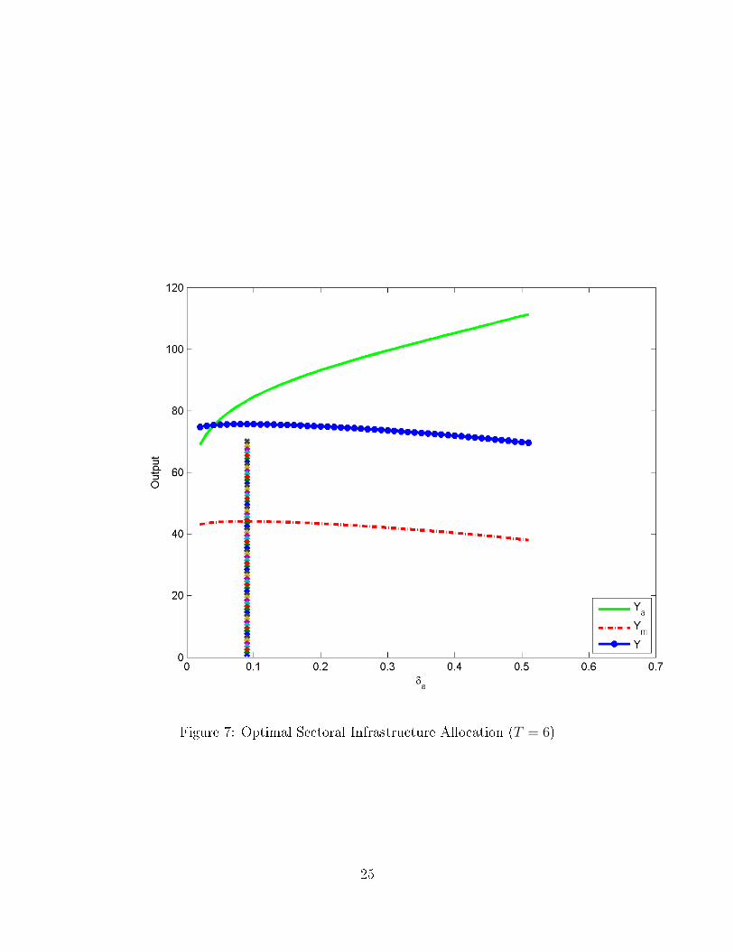
We �nd: First, the share of infrastructure going to agriculture that is GDP maxi-

mizing is rather small at around 10%. Consequently, larger public investment shares

in agriculture would not increase GDP, but only serve to depress the agricultural

price. Second, the e�ects of increasing the agricultural consumption subsidy holding

the other expenditure levels constant are qualitatively very similar to the e�ect of

increasing agriculture's share of infrastructure investment. A high subsidy of agri-

cultural consumption shifts resources away from manufacture into agriculture, which

depresses employment, capital accumulation and output in the former sector. Third,

manufacturing output is hump shaped in the fraction of public investment going to

agriculture. Evidently, the manufacturing sector bene�ts in terms of output from a

modest agricultural investment that supports a relatively sizeable agricultural sector.

Fourth, GDP is hump-shaped in public infrastructure funding. The growth maximiz-

ing funding level for infrastructure investment is much larger than the one suggested

by one-sector growth models. Exogenous �scal policies thus can thus potentially

play an important role in accounting for structural transformation in sectoral output

shares, sectoral capital-output ratios, and sectoral employment shares in the Indian

context.

4

2 The Model

The economy is populated by an in�nite number of generations. Each generation is

alive for two periods. The two periods are young age and old age, each accounts for 25

years. All individuals work when young and are retired when old. Within a generation

all individuals are identical. For simplicity we assume that all individuals consume

only in the second period of life. Thus all income from the �rst period is saved for

consumption when old. There are two sectors, one we call "agriculture" and a second

sector we call "manufacturing", although the names are not crucial. What is crucial

is that there are two sectors, with one sector declining and one sector increasing along

the development path. We chose a utility function which helps generate one declining

and one rising sector in equilibrium, namely the semi-linear utility function. The

utility function for all households is given by:

u(cm,t+1, ca,t+1) = cm,t+1 + φlnca,t+1, φ > 0, (2.1)

where cm,t+1 denotes the household consumption of the manufacturing good and ca,t+1

the consumption of the agricultural good. The semi-linear utility also captures the

observation that the income elasticities for the demand for food are (close to) zero.

Households working in the agricultural sector solve the following problem:

maxcm,ca

cm,t+1 + φlnca,t+1,

s.t. cm,t+1 + (1− ξ)pt+1ca,t+1 = (1− τa)ptwa,t(1 + rt)(2.2)

Here wa,t is the real wage rate, rt is the real interest rate, pt and pt+1 are the

prices of agricultural good relative to the manufacturing good in period t and t + 1

respectively, and ξ is the excise subsidy applied to agricultural goods.

Households working in the manufacturing sector solve the following problem:

5

maxcm,ca

cm,t+1 + φlnca,t+1,

s.t. cm,t+1 + (1− ξ)pt+1ca,t+1 = (1− τm)wm,t(1 + rt)(2.3)

The only di�erence in the two household problems are the sources of income.

Solving the problem of the households in the agricultural sector yields the demand

for the two consumption goods as:

caa,t+1 =φ

(1− ξ)pt+1

cam,t+1 = (1− τa)ptwa,t(1 + rt)− φ(2.4)

Similarly, the manufacturing sector households solve their maximization problem

which yields their demand function as:

cma,t+1 =φ

(1− ξ)pt+1

cmm,t+1 = (1− τm)wm,t(1 + rt)− φ(2.5)

The production functions in both sectors are:

Aa,tGψaa,tK

αa,tL

1−αa,t (2.6)

Am,tGψmm,tK

βm,tL

1−βm,t (2.7)

Here Aa,t and Am,t are total-factor-productivity (TFP) in the agricultural and

manufacturing sectors, respectively. Ka,t and Km,t are the total amount of physical

capital used and La,t and Lm,t stand for the total amount of labor employed in the

two sectors. Lastly, the production of the agricultural and manufacturing goods is

augmented by an investment in a public good (infrastructure), denoted by Ga,t and

6

Gm,t. The use of these types of technologies with public capital as an input was

pioneered by Barro (1990) and Turnovsky (1996) and others. We assume that such

investments in public infrastructure can be �nanced by a tax on (1) labor income in

the manufacturing sector, or (2) labor income in the agriculture sector, or (3) both.

In addition to �nancing the public good investment, the government also subsidies

consumption of agricultural products.

The government budget constraint can be written as

Ga,t +Gm,t + ξptca,t = τawa,tLa,t + τmwm,tLm,t (2.8)

where ξ is the subsidy for agricultural goods consumption. Note that τa ≥ 0 and

τm ≥ 0. We do not allow public debt in our model.

Letting δa ∈ [0, 1] denote the fraction of government revenue which is allocated to

agricultural infrastructure, we can write

Ga,t = δa[τawa,tLa,t + τmwm,tLm,t − ξptca,t] (2.9)

Gm,t = (1− δa)[τawa,tLa,t + τmwm,tLm,t − ξptca,t] (2.10)

The returns to factors in the two sectors are:

wa,t = (1− α)Aa,tGψaa,t(Ka,t/La,t)

α (2.11)

wm,t = (1− β)Am,tGψmm,t(Km,t/Lm,t)

β (2.12)

qa,t = αAa,tGψaa,t(Ka,t/La,t)

α−1 (2.13)

qm,t = βAm,tGψmm,t(Km,t/Lm,t)

β−1 (2.14)

Assuming costless mobility of labor, we can equate the wage rates across the two

7

sectors:

(1− τa)pt(1− α)Aa,tGψaa,t(Ka,t/La,t)

α = (1− τm)(1− β)Am,tGψmm,t(Km,t/Lm,t)

β (2.15)

Similarly, we equate interest rates across the two sectors:

ptαAa,tGψaa,t(Ka,t/La,t)

α−1 = βAm,tGψmm,t(Km,t/Lm,t)

β−1 (2.16)

The market clearing condition for the two goods are:

caa,tLa,t−1 + cma,tLm,t−1 = AaGψaa,tK

αa,tL

1−αa,t

cam,tLa,t−1 + cmm,tLm,t−1 = AmGψmm,tK

βm,tL

1−βm,t

(2.17)

The law of motion for capital:

Ka,t+1 +Km,t+1 = (1− τa)ptwa,tLa,t + (1− τm)wm,tLm,t (2.18)

Note that households only consume in the second period of life, therefore all income

is saved and funds the future capital stock. We assume that there is no population

growth so that the labor force is constant over time. Assuming competitive labor

markets, the labor allocations in the two sectors must add up to the total labor

supply.

La,t + Lm,t = Lt

Lt = Lt+1

(2.19)

3 Results

3.1 Overall e�ects in the long run

In this section we describe how changes in �scal policy measures in�uence the equi-

librium trajectories. Here we focus on the qualitative e�ects of the following policy

8

reforms:

1. Increasing the share of infrastructure investment going to agriculture (δa) with

a corresponding decrease in manufacturing's share (δm).

2. Increasing the agricultural subsidy (ξ), holding both tax rates constant.

3. Raising the agricultural tax (τa), while increasing all government expenditure

proportionately, holding the manufacturing tax rate �xed.

4. Raising the manufacturing tax (τm), while increasing all government expendi-

tures proportionately, holding the agricultural tax rate �xed.

5. Increasing both tax rates simultaneously, holding all expenditure shares con-

stant.

The parameter values used for our simulations are presented in Table 2. These

values, such as the income shares of capital and other production function parameters,

are standard in the literature. For India-speci�c values, such as the level and growth

rate of Total Factor Productivity (TFP), we have followed Verma (2012). The long

term trajectories are illustrated in Figures (1)-(4). Under the economic and policy

parameters chosen for the simulations, the dynamic equilibrium results generated by

our model are very similar with the data from Verma (2012). In particular aggregate

capital, aggregate labor, GDP and both sectoral outputs are increasing over time.

The fraction of labor employed in agriculture is declining over time, agriculture's

share of GDP is declining over time. Interestingly and consistent with the data, the

capital-output ratio falls in agriculture and rises in manufacturing over time. The

model matches the data for all �scal policies chosen for our simulations.

As is evident from Figure (1), increasing the share of agricultural infrastructure

investment from 0.1 to 0.4 shifts both capital and labor from manufacturing into

agriculture. As a consequence agricultural output rises, while manufacturing output

falls. The price of the agricultural good falls. The negative e�ect on manufacturing

outweighs the positive e�ect on agriculture and therefore overall GDP falls. The

e�ects of shifting infrastructure towards agriculture on the overall GDP are very

9

small. The four-fold increase in agriculture's share of infrastructure decreases GDP

after six periods only by 5.3%.

The e�ects of increasing the agricultural subsidy, see Figure (2), are qualitatively

very similar to the e�ect of increasing agriculture's share of infrastructure investment.

A high agricultural subsidy shifts resources away from manufacture into agriculture,

which depresses employment, capital accumulation and output in the former sector.

Quantitatively increasing the size of the agricultural subsidy on GDP seems very

small.

Figure (3) shows that, raising the tax rate in the agricultural sector massively

shifts resources out of the agricultural sector, agricultural output falls, manufacturing

output rises and overall GDP increases. The relative price of food rises. This e�ect

is large. Raising the tax on income from the manufacturing sector (see Figure (4)) is

just the �ip side of the policy considered in Figure (3). Since the income elasticity

for the agricultural good is zero and the income elasticity for the manufacturing good

is positive, we can think of manufacturing as the "dynamic" sector and agriculture

as the "stagnant" sector. From these last two experiments we learn that increasing

taxes on the stagnant (dynamic) sector increases (decreases) GDP.

3.2 Optimal split of government funding between two sectors

- δa

One of the important policy issues we consider is how public infrastructure investment

should be split between the modern dynamic manufacturing sector and the more tra-

ditional agricultural sector. Holding all other dimensions of �scal policy constant we

change the share of the infrastructure capital going to agriculture rather than man-

ufacturing and compute how the GDP growth rate depends upon δa. We calculate

the level of δa which maximizes the level of GDP. We do this in periods two, four and

six, and the corresponding results are illustrated in Figures (5), (6), and (7). What

stands out in these �gures is that the share of infrastructure going to agriculture

that is GDP maximizing is rather small at around 10%. This small fraction re�ects

the fact that given the speci�ed utility function the income elasticity for the demand

10

for the agricultural good is zero. Notice that in this experiment both coe�cients on

infrastructure in the two sectoral production functions are the same. With symmetric

treatment of both goods in the utility function the output maximizing share of agri-

cultural infrastructure will be around 50%. The small size of the optimal agricultural

share in infrastructure is entirely due to the semi-linear nature of the utility function.

Consequently larger public investment shares in agriculture would not increase GDP,

but only serve to depress the agricultural price. It is also noteworthy that this output

maximizing fraction stays rather constant at 10% over time even as the agricultural

sector shrinks relative to the modern manufacturing sector. Surprisingly, manufactur-

ing output is hump shaped in the fraction of public investment going to agriculture.

One might have expected that shifting resources away from manufacturing uniformly

decreases manufacturing output, but evidently the manufacturing sector bene�ts in

terms of output from a modest agricultural investment that supports a relatively

sizeable agricultural sector.

3.3 Optimal tax rates

To �nd the optimal tax rates, we conduct the following experiments:

1. Raising the agricultural tax rate (τa), while holding the manufacturing tax rate

(τm) constant.

2. Raising the manufacturing tax rate (τm), while holding the agricultural tax rate

(τa) constant.

3. Raising the two tax rates (τa, τm) at the same time.

When we vary the agricultural tax rate holding the manufacturing tax rate and

the split of infrastructure between the two sectors constant, the results are illustrated

in Figure (8). Increasing the agricultural tax rate decreases agricultural output and

increases manufacturing output by shifting resources out of agriculture sector. Since

the manufacturing sector is the dynamic sector, this policy increases the growth

rate of overall GDP. The results of increasing the tax in the manufacturing sector,

11

which are illustrated in Figure (9), are diametrically opposite: there is a decrease in

manufacturing output, an increase in agricultural production and a decrease in overall

GDP. Varying the sectoral tax rates has very large e�ects. Increasing the agricultural

tax rate from about 20% to 50% increases the level of GDP by over 40%. Similarly

large e�ects are found for changes in the manufacturing tax rate. Getting the sectoral

allocation of these tax burdens right thus has potentially large e�ects on GDP and

therefore on welfare.

Varying the two tax rates τa and τm simultaneously has the expected e�ects as

seen in Figure (10). Increasing the manufacturing tax rates decreases the level of

output, while increasing the agricultural tax rate increases the output level. Varying

both tax rates has the expected composite e�ect.

In Barro (1990) and similar papers the relationship between the funding level for

public infrastructure and the growth rate (or the level) of GDP is hump-shaped with

the peak occurring when the tax rate is equal to the coe�cient on public capital in the

production function. We now investigate to what extent that result carries over to the

two-sector setting. Since we have two tax rates we have to �x the relationship between

the two tax rates. First we set the agricultural tax rate equal to the manufacturing

tax rate and then increase both rates proportionately. As is illustrated in Figure (11),

this policy leads to a monotonic relationship between the tax rate and the growth rate

of GDP. Higher tax rates are associated with higher levels of income over the entire

relevant range suggested by the size of the infrastructure productivity coe�cients.

We next set τm = 1.5τa and scale up the size of the government. In this case, see

Figures (12)-(14), the relationship between tax rates and the level of income turns out

to be hump shaped. As the tax rates are increased, the size of agricultural production

rises, manufacturing output is hump shaped in the tax rates. Putting these e�ects

together generates the hump shaped relationship between tax rates and overall GDP.

It is noteworthy that the tax rate which maximizes the level of GDP is substantially

larger than the infrastructure coe�cient in the production function (ψa = ψm = 0.12

in this experiment). Moreover, it is apparent from Figures (12)-(14) that, unlike in

Barro (1990), the tax rate which maximizes GDP is not constant, but rising over

time. As the relative role of agriculture shrinks and the role of the modern dynamic

12

manufacturing sector rises, the funding requirement for public infrastructure rises as

well so that the GDP maximizing funding level increases over time.

In Figure (15), we show how the GDP maximizing tax rate depends upon the

infrastructure productivity coe�cients ψa and ψm assuming they are equal. If a

Barro like result had obtained in our model, the maximizing tax rate would line up

on the 45 degree line. As we can see from Figure (15), the maximizing tax rate is

higher than the one in Barro (1990) and the gap between the 45 degree line and the

GDP maximizing funding level increases as public capital becomes more productive.

4 Sensitivity analysis

In order to investigate the robustness of our results we relax the Cobb-Douglas as-

sumption for the production technologies and allow the manufacturing technology to

be of the CES variety. The production function is given by

Ym,t = Am,tGψmm,t((1− θ)K

ρm,t + θLρm,t)

1ρ , −∞ < ρ < 1 (4.1)

We now let the parameter ρ vary from -100 (almost perfect complements) to 0.5

(very close substitutes). In Figures (16)-(18) we illustrate how the output maximizing

share of public investment going to agriculture as opposed to manufacturing depends

upon the elasticity of substitution parameter ρ. The result is remarkably robust: For

all the values of ρ ranging from -100 to 0.5, the output maximizing share going to

agriculture is very close to 0.1. Figure (16) illustrates the case for T = 2. We have

also run this experiment for T = 4 and T = 6. The results for these two other periods

are basically the same.

In Figures (19)-(21) we show how output depends upon the change in the overall

tax rate for the same values of ρ going from -100 to 0.5. The case for period t = 2 is

illustrated in Figure (19). As ρ increases from -100 to 0.5 the output maximizing tax

rate rises from about 0.22 to about 0.24. This sensitivity is slightly more pronounced

in later periods. In period T = 6 (see Figure Figures (21)) the output maximizing

tax rate goes from around 0.25 to almost 0.3.

13

5 Conclusion

We constructed a tractable two-sector model to study the e�ects of sectoral infrastruc-

ture allocations on economic growth. The model we use �ts the growth observations

for Indian as documented by Verma (2012). In our simulations we show that pub-

lic infrastructure policies can play an important role in in�uencing the allocation of

private capital and labor across sector, which then in turn has a powerful in�uence

on overall economic growth. In particular we establish: First, the growth maximiz-

ing allocation of infrastructure invest to the agricultural sector is small. Second, the

growth e�ects of agricultural subsidies are large. Third, sectoral taxation can have

very large e�ects on economic growth. Lastly, the growth maximizing infrastructure

funding level is much larger than that suggested by the one sector growth model.

In this paper we have used the competitive market assumption and abstracted

from a variety of distortions in factor markets such as large public sector involvement

in the manufacturing production. We leave such extensions for future work.

14

References

[1] Agénor, P.R., 2008, "Fiscal Policy and Endogenous Growth with Public Infras-

tructure," Oxford Economic Papers, 60:57-87.

[2] Agénor, P.R., and Moreno-Dodson, B., 2006, "Public Infrastructure and

Growth: New Channels and Policy Implications," World Bank Policy Research

Working Paper No. 4064. http : //ssrn.com/abstract = 943921

[3] Ai, C., and Cassou, S.P., 1995, "A Normative Analysis of Public Capital,"

Applied Economics, 27:1201-1209.

[4] Angelopoulos, K., Economides, G., and Kammas, P., 2007, "Tax-Spending Poli-

cies and Economic Growth: Theoretical Predictions and Evidence from the

OECD," European Journal of Political Economy, 23:885-902.

[5] Arcalean, C., Glomm, G., and Schiopu, I., 2009, "Growth E�ects of Spa-

tial Redistribution Policies," CAEPR Working Paper No. 2007-002. http :

//ssrn.com/abstract = 960475

[6] Aschauer, D.A., 1989, "Is Public Expenditure Productive?" Journal of Mone-

tary Economics, 23:177-200.

[7] Banga, R., 2005, "Critical Issues in India's Service-Led Growth," Indian Council

for Research, Working Paper No. 171. http : //www.icrier.org/pdf/WP171.pdf

[8] Barro, R.J., 1991, "Economic Growth in a Cross Section of Countries," The

Quarterly Journal of Economics, 106:407-443.

[9] Barro, R.J., 1990, "Government Spending in a Simple Model of Endogenous

Growth," Journal of Political Economy, 98:S103-S125.

[10] Bhattacharjea, A., 2006, "Labour Market Regulation and Industrial Perfor-

mance in India: A Critical Review of the Empirical Evidence," Indian Journal

of Labour Economics, 39:211-232.

15

[11] Caminal, R., 2004, "Personal Redistribution and the Regional Allocation of

Public Investment," Regional Science and Urban Economics, 34:55-69.

[12] Carrera, J.A., Freire-Seren, M.J., and Manzano, B., 2000, "Macroeconomic Ef-

fects of the Regional Allocation of Public Capital Formation," Regional Science

and Urban Economics, 39:563-574.

[13] Casella, A., 2005, "Redistribution Policy: A European Model," Journal of Pub-

lic Economics, 89:1305-1331.

[14] Caselli, F., and Coleman, W.J., 2001, "The U.S. Structural Transformation

and Regional Convergence: A Reinterpretation," Journal of Political Economy,

109:584-616.

[15] de la Fuente, A., Vives, X., Dolado, J.J., and Faini, R., 1995, "Infrastructure

and Education as Instruments of Regional Policy: Evidence from Spain," Eco-

nomic Policy, 10:11-51.

[16] Eicher, T.S., 2000, "Scale, Congestion and Growth," Economica, 67:325-346.

[17] Fisher, W.H., and Turnovsky, S.J., 1998, "Public Investment, Congestion, and

Private Capital Accumulation," The Economic Journal, 108:399-413.

[18] Glomm, G., and Ravikumar, B., 1997 "Productive Government Expenditures

and Long-Run Growth," Journal of Economic Dynamics and Control, 21:183-

204.

[19] Glomm, G., and Ravikumar, B., 1994, "Public Investment in Infrastructure in

a Simple Growth Model," Journal of Economic Dynamics and Control, 18:1173-

1187.

[20] Glomm, G., 1992, "A Model of Growth and Migration," Canadian Journal of

Economics, 25:901-922.

[21] Gollin, D., Parente, S., and Rogerson, R., 2002, "The Role of Agriculture in

Development," American Economic Review, 92:160-164.

16

[22] Holtz-Eakin, D., 1994, "Public-Sector Capital and the Productivity Puzzle,"

Review of Economics and Statistics, 76:12-21.

[23] Laitner, John, 2000, "Structural Change and Economic Growth," Review of

Economic Studies, 67: 545-561.

[24] Lucas, R.E.J., 2004, "Life Earnings and Rural-Urban Migration," Journal of

Political Economy, 112:29-59.

[25] Lynde, C., and Richmond, J., 1992, "The Role of Public Capital in Production,"

Review of Economics and Statistics, 74:37-44.

[26] Maddison, A., 1982, Phases of Capitalist Development, Oxford: Oxford Uni-

versity Press.

[27] Marathe, S.S., 1986, Regulation and Development: India's Policy Experience

of Controls Over Industry, Sage Publications: New Delhi.

[28] Ott, I., and Soretz, S., 2010, "Productive Public Input, Integration and Ag-

glomeration," Regional Science and Urban Economics, 40:538-549.

[29] Ott, I., and Turnovsky, S.J., 2006, "Excludable and Non-excludable Public

Inputs: Consequences for Economic Growth," Economica, 73:725-748.

[30] Suedekum, J., 2005, "the Pitfalls of Regional Education Policy," FinanzArchiv:

Public Finance Analysis, 61:327-352.

[31] Turnovsky, S., 1996, "Optimal Tax, Debt, and Expenditure Policies in a Grow-

ing Economy," Journal of Public Economics, 60:21-44.

[32] Turnovsky, S., and Fischer, W., 1995 "The Composition of Government Ex-

penditure and Its Consequences for Macroeconomic Performance," Journal of

Economic Dynamics and Control, 19:747-786.

[33] Verma, R., 2012, "Structural Transformation and Jobless Growth in the Indian

Economy," The Oxford Handbook of the Indian Economy, Oxford University

Press.

17

Table 1: DataAgriculture Manufacturing Services1970 2000 1970 2000 1970 2000

Employment Shares(a) 77% 62% 12% 19% 12% 20%GDP Shares 48% 25% 23% 27% 29% 48%K/Y Ratios 3.3 0.85 0.6 4.33 11 1.82Gross Capital Formation 18% 9% 33% 30% 49% 61%

Source: Verma(2012)(a): the employment share data are for 1970 and 1997.

Table 2: Calibration ValuesDe�nition Normal Experiments

1 2 3 4

Aa initial TFP in agriculture 2Am initial TFP in manufacturing 1ga growth rate of agri TFP (20 yrs) 1.2gm growth rate of manuf TFP (20 yrs) 1.05α income share of K in agri 0.3β income share of K in manuf 0.4φ parameter in consumption func 2ψa power param of G in agri prod. 0.12∼ 0.2ψm power param of G in manuf prod. 0.12∼ 0.2

δa govt funding share for agri 0.5 {0.1, 0.4}ξ govt subsidy of agricultural prices 0.05 {0.01, 0.1}τa tax rate of agricultural income 0.3 {0.2,0.4}τm tax rate of manufacturing income 0.3 {0.01,0.35}

18

Figure 1: Policy experiment 1: raising δa (allocation of govt funding to agriculture)from 0.1 to 0.4. Green: agriculture; Red: Manufacturing; Solid line: before experi-ment; Dashed line: after experiment.

19

Figure 2: Policy experiment 2: raising ξ (subsidies of agriculture goods) from 0.01 to0.1. Green: agriculture; Red: Manufacturing; Solid line: before experiment; Dashedline: after experiment.

20

Figure 3: Policy experiment 3: raising τa (income tax rate on agricultural workers)from 0.2 to 0.4. Green: agriculture; Red: Manufacturing; Solid line: before experi-ment; Dashed line: after experiment.

21

Figure 4: Policy experiment 4: raising τm (income tax rate on manufacturing work-ers) from 0.01 to 0.35. Green: agriculture; Red: Manufacturing; Solid line: beforeexperiment; Dashed line: after experiment.

22

Figure 5: Optimal Sectoral Infrastructure Allocation (T = 2)

23

Figure 6: Optimal Sectoral Infrastructure Allocation (T = 4)

24

Figure 7: Optimal Sectoral Infrastructure Allocation (T = 6)

25

Figure 8: Varying agricultural tax rate, while holding manufacturing tax rate con-stant. (T = 2)

26

Figure 9: Varying manufacturing tax rate, while holding agricultural tax rate con-stant. (T = 2)

27

Figure 10: Output E�ects of Changes in Both Tax Rates (T=2)Note: Output is an increasing function of τa and a decreasing function of τm.

28

Figure 11: Optimal E�ects of Simultaneous Changes in the Two Tax Rates (T = 2,τm = τa)

29

Figure 12: Optimal E�ects of Simultaneous Changes in the Two Tax Rates (T = 2,τm = 1.5τa)

30

Figure 13: Optimal E�ects of Simultaneous Changes in the Two Tax Rates (T = 4,τm = 1.5τa)

31

Figure 14: Optimal E�ects of Simultaneous Changes in the Two Tax Rates (T = 6,τm = 1.5τa)

32

Figure 15: Output Maximizing Tax Rates for Varying Levels of ψ (T = 2, ψa =ψm, τm = 1.5τa)

33

Figure 16: Output Maximizing δa for the CES Production Function (T = 2)

34

Figure 17: Output Maximizing δa for the CES Production Function (T = 4)

35

Figure 18: Output Maximizing δa for the CES Production Function (T = 6)

36

Figure 19: Output E�ects of Simultaneous Changes in the Tax Rates for the CESProduction Function (T = 2, τm = 1.5τa)

37

Figure 20: Output E�ects of Simultaneous Changes in the Tax Rates for the CESProduction Function (T = 4, τm = 1.5τa)

38

Figure 21: Output E�ects of Simultaneous Changes in the Tax Rates for the CESProduction Function (T = 6, τm = 1.5τa)

39

Working Paper No. 236

INDIAN COUNCIL FOR RESEARCH ON INTERNATIONAL ECONOMIC RELATIONS

LATEST ICRIER’S WORKING PAPERS

NO. TITLE

AUTHOR YEAR

261

WHY WAS THE PARTICIPATION OF INDIAN STATES IN THE GROWTH TURNAROUND SO PATCHY? SOME EVIDENCE BASED ON ROBUSTNESS ANALYSIS

CHETAN GHATE AND STEPHEN WRIGHT

OCTOBER 2012

260

HAS INDIA EMERGED? BUSINESS CYCLE STYLIZED FACTS FROM A TRANSITIONING ECONOMY

CHETAN GHATE RADHIKA PANDEY ILA PATNAIK

JUNE 2012

259

AN ASSESSMENT OF INFLATION MODELLING IN INDIA

B. KARAN SINGH APRIL 2012

258

TOWARD A FRAMEWORK FOR IMPLEMENTATION OF CLIMATE CHANGE TREATY THROUGH SELF-ENFORCING MECHANISMS

MEETA KESWANI MEHRA SAPTARSHI MUKHERJEE MONICA DUTTA

JANUARY 2012

257

INDIA’S EXPERIENCE IN

NAVIGATING THE TRILEMMA: DO CAPITAL CONTROLS HELP?

R. KOHLI JUNE 2011

256

MONETARY POLICY AND CREDIT DEMAND IN INDIA AND SOME EMES

B L PANDIT PANKAJ VASHISHT

MAY 2011

255

ENHANCING INTRA-SAARC TRADE: PRUNING INDIA’S SENSITIVE LIST

UNDER SAFTA

NISHA TANEJA SAON RAY NEETIKA KAUSHAL DEVJIT ROY CHOWDHURY

APRIL 2011

254

FINANCIAL TRANSACTIONS TAXES

PARTHASARATHI SHOME

APRIL 2011

253

INDIAN ECONOMY: SELECTED METHODOLOGICAL ADVANCES

MATHEW JOSEPH KARAN SINGH RANJAN KUMAR DASH JYOTIRMOY BHATTACHARYA RITIKA TEWARI

FEBRUARY 2011

252

HEALTHCARE DELIVERY AND STAKEHOLDER’S SATISFACTION

UNDER SOCIAL HEALTH INSURANCE SCHEMES IN INDIA: AN EVALUATION OF CENTRAL GOVERNMENT HEALTH SCHEME (CGHS) AND EX-SERVICEMEN CONTRIBUTORY HEALTH SCHEME (ECHS)

SUKUMAR VELLAKKAL SHIKHA JUYAL ALI MEHDI

DECEMBER 2010

1

Working Paper No. 236

INDIAN COUNCIL FOR RESEARCH ON INTERNATIONAL ECONOMIC RELATIONS

About ICRIER

Established in August 1981, ICRIER is an autonomous, policy-oriented, not-for-profit, economic policy think tank. ICRIER's main focus is to enhance the knowledge content of policy making by undertaking analytical research that is targeted at informing India's policy makers and also at improving the interface with the global economy. ICRIER's office is located in the institutional complex of India Habitat Centre, New Delhi. ICRIER's Board of Governors include leading academicians, policymakers, and representatives from the private sector. Dr. Isher Ahluwalia is ICRIER's chairperson. Dr. Rajat Kathuria is Director and Chief Executive. ICRIER conducts thematic research in the following seven thrust areas:

Macro-economic Management in an Open Economy Trade, Openness, Restructuring and Competitiveness Financial Sector Liberalisation and Regulation WTO-related Issues Regional Economic Co-operation with Focus on South Asia Strategic Aspects of India's International Economic Relations Environment and Climate Change

To effectively disseminate research findings, ICRIER organises workshops, seminars and conferences to bring together academicians, policymakers, representatives from industry and media to create a more informed understanding on issues of major policy interest. ICRIER routinely invites distinguished scholars and policymakers from around the world to deliver public lectures and give seminars on economic themes of interest to contemporary India.


Recommended