Securitization and House Price Growth 1 Genevieve Nelson 2 University of Oxford December 31, 2019 Job Market Paper Please click here for latest version Abstract From 2000-2006 US house prices and mortgage credit grew substantially. Simultaneously, the relative cost of mortgage credit fell – particularly for privately securitized mortgages – suggesting the importance of credit supply factors. This paper explores two candidate (credit supply) shocks: an increase in the inflow of global savings into the US, and innovations in the securitization of mortgage credit. I model a two-layered mortgage market. This generates a novel balance sheet effect : changes in aggregate mortgage credit quantity are linked to changes in mortgage spreads via the interaction of financially constrained commercial banks and mortgage securitizers. Innovation in securitization matches mortgage credit market dynamics by directly relaxing the securitizers’ financial constraint. Conversely, the inflow of global savings leads to a counter-factual increase of mortgage spreads through the balance sheet effect. Keywords: Securitization, Mortgage Credit, House Prices, Non-Banks. JEL Codes: G01, G21, G23, E21, E44 1 I thank my advisor Andrea Ferrero for his guidance and support, as well as Michael McMahon, Andrea Tambalotti, Jeffrey Campbell and Jose Dorich. And James Vickery for helpful conversations and facilitating my access to data. For helpful discussions I thank Martin Ellison, Francesco Zanetti, Petr Sedlacek, Hamish Low, Klaus Adams, Guido Ascari, Myrto Oikonomou, Alexander Haas, Andrew Haughwout, Anna Kovner, Argia Sbordone, Nina Boyarchenko, David Lucca, Marco Del Negro, Keshav Dogra, Anna Paulson, Leonardo Melosi, Richard Rosen, Stefania D’Amico, Robert Barsky, Richard Harrison, David Aikman, Kristina Bluw- stein, Lien Laureys, Thomas Carter, Jason Allen, and H´ el` ene Desgagn´ es. This paper benefited greatly from time spent, presentations and many conversations with economists at the Bank of Canada, the Bank of England, the Federal Reserve Bank of Chicago and Federal Reserve Bank of New York. The views expressed in this paper are entirely my own as are any remaining errors. 2 University of Oxford, Manor Road Building, Manor Road, Oxford OX1 3UQ, [email protected]
Transcript
Securitization and House Price Growth1
Genevieve Nelson2University of Oxford
December 31, 2019
Job Market PaperPlease click here for latest version
Abstract
From 2000-2006 US house prices and mortgage credit grew substantially. Simultaneously, the
relative cost of mortgage credit fell – particularly for privately securitized mortgages – suggesting
the importance of credit supply factors. This paper explores two candidate (credit supply) shocks:
an increase in the inflow of global savings into the US, and innovations in the securitization of
mortgage credit. I model a two-layered mortgage market. This generates a novel balance sheet
effect : changes in aggregate mortgage credit quantity are linked to changes in mortgage spreads via
the interaction of financially constrained commercial banks and mortgage securitizers. Innovation
in securitization matches mortgage credit market dynamics by directly relaxing the securitizers’
financial constraint. Conversely, the inflow of global savings leads to a counter-factual increase of
mortgage spreads through the balance sheet effect.
Keywords: Securitization, Mortgage Credit, House Prices, Non-Banks.
JEL Codes: G01, G21, G23, E21, E44
1I thank my advisor Andrea Ferrero for his guidance and support, as well as Michael McMahon, AndreaTambalotti, Jeffrey Campbell and Jose Dorich. And James Vickery for helpful conversations and facilitatingmy access to data. For helpful discussions I thank Martin Ellison, Francesco Zanetti, Petr Sedlacek, HamishLow, Klaus Adams, Guido Ascari, Myrto Oikonomou, Alexander Haas, Andrew Haughwout, Anna Kovner,Argia Sbordone, Nina Boyarchenko, David Lucca, Marco Del Negro, Keshav Dogra, Anna Paulson, LeonardoMelosi, Richard Rosen, Stefania D’Amico, Robert Barsky, Richard Harrison, David Aikman, Kristina Bluw-stein, Lien Laureys, Thomas Carter, Jason Allen, and Helene Desgagnes. This paper benefited greatly fromtime spent, presentations and many conversations with economists at the Bank of Canada, the Bank ofEngland, the Federal Reserve Bank of Chicago and Federal Reserve Bank of New York. The views expressedin this paper are entirely my own as are any remaining errors.
The Great Recession was preceded by an unprecedented 48% boom in US real house prices
from 2000 to 2006. In contrast during the “Baby Boom” period from 1946 - 1964 real
house price growth peaked at 33%. US mortgages were increasingly being held not by
regulated commercial banks or the implicitly government backed Fannie Mae and Freddie
Mac but by the shadow banking sector. The vehicle for this shift was private mortgage
backed securitization3. The issuance of private mortgage backed securities grew from 126
Billion USD in 2000 to 1,145 Billion USD in 2006. This period was a culmination of a
series of “innovations” in private securitization, including increased use of tranching4 and
other credit enhancements, which drove investor willingness to treat private sector issued
mortgage backed securities as nearly substitutable to US Treasuries. My paper explores the
role of a securitization driven credit supply expansion during this period. My key finding is
that innovation in securitization drove at least 71% of the house price appreciation and 34 -
45% of the increase in non-conforming mortgage credit during this period.
The contribution of this paper is to explicitly model the private securitization of mortgage
credit. By doing so I get a new balance sheet effect missed by standard models. In my model
financial intermediaries face constraints on the size and composition of their balance sheets.
Shadow banks (the issuers of mortgage backed securities) face a constraint which limits the
total quantity of mortgage credit they can hold, relative to the profits (i.e. spread) they make.
They cannot exceed this limit because their liabilities (mortgage backed securities) would go
from being perceived as risk-less to being perceived as too risky to hold. Commercial banks
face a solvency constraint. This constraint forces them to diversify their assets by selling
the (idiosyncratically risky) mortgages they issue and buying mortgage backed securities
(which only have aggregate risk). The aggregate constraint on shadow banks is the ultimate
constraint on aggregate mortgage credit that the financial sector can absorb at a given
mortgage spread. Because of the balance sheet effect a relaxation of the constraint faced
3Securitization is the process of a financial entity buying a group of mortgages and issuing an asset, themortgage backed security (MBS), that pays out based on the underlying income stream from those mortgagesas borrowers repay.
4When you buy a mortgage backed security you can buy the right to be paid off first (senior tranche) orlast (equity tranche). Tranches are essentially your position in line to be paid back as borrowers repay theirmortgages.
1
by shadow banks is needed to explain the decline in mortgage spreads and increase in total
mortgage credit in the 2000 - 2006 U.S. data. This is “innovation in securitization”.
The U.S. experience of the Financial Crisis opened up a debate as to whether positive
shifts in credit demand or credit supply drove the boom in US house prices and mortgage
debt between 2000 and 2006. On credit demand, researchers suggest that some non-financial
factors, for example: optimism about future house prices (Kaplan, Mitman and Violante,
2017), or a speculative bubble (Shiller, 2007) drove an increase in house prices which in
turn drove an increase in the demand for credit – to finance the purchase of more expensive
housing. The credit supply view, advanced by Mian and Sufi (2017) and Justiniano, Primiceri
and Tambalotti (2019), points to the large increase in the quantity of mortgage credit along
with a decrease in the relative cost of mortgage credit, suggesting that the boom was driven
by a positive shift in credit supply (Figure 1).
Figure 1: Credit Supply View - Key Stylized Facts
1995 2000 2005 2010 201560
80
100
120
140
160
180
Index,20
00Q4=10
0
(a) Boom in Mortgage Credit
Non-Conforming/GDP
All Mortgages/GDP
2000 2001 2002 2003 2004 2005 2006
2
3
4
5
Spread
over
10YearTreasury
(b) Compression of Mortgage Spreads
Non-ConformingConforming
(a) All Mortgages/GDP: The total outstanding stock of mortgage credit relative to GDP, indexed to 2000Q4levels. Non-Conforming/GDP: Estimated as “All Mortgages” minus those mortgages held by GovernmentSponsored Enterprises (GSEs) and GSE & Agency backed pools, relative to GDP, indexed to 2000Q4 levels.Source: Board of Governors of the Federal Reserve System (US), Z1 Financial Accounts of the UnitedStates, retrieved from DDP; www.federalreserve.gov/datadownload/, August 15, 2019.(b) Conforming: Board of Governors of the Federal Reserve System (US), 30-Year Conventional Mort-gage Rate (DISCONTINUED) [MORTG], retrieved from FRED, Federal Reserve Bank of St. Louis;https://fred.stlouisfed.org/series/MORTG, September 1, 2019. Non-Conforming: average mortgage rateat origination for the near-universe of privately securitized mortgages, source: Justiniano, Primiceri, &Tambalotti (2017).
Capturing the balance sheet effect is key to distinguishing between different potential
2
drivers of the expansion in credit supply. A generic credit supply shift, driven by an increase
in savers’ demand for deposits, drives commercial banks to increase the size of their balance
sheet. Commercial banks issue more mortgage credit but also demand more mortgage backed
securities. This is because the financial constraint faced by commercial banks penalizes them
for holding their own originated mortgages. They choose to sell a portion of these mortgages
and hold mortgage backed securities instead. In this way the generic credit supply shock
translates into an increase in demand for mortgage backed securities - driving mortgage
spreads up because of the balance sheet effect. Furthermore the balance sheet effect magnifies
the positive impact on the mortgage spread that a credit demand shift (“Housing Demand”
shock) would have.
Not only is the the innovation in securitization channel necessary to explain mortgage
spread dynamics in the 2000 - 2006 data, it could have set the stage to amplify other
potential factors driving credit dynamics during this period. I show that, in a world where
mortgage securitizers face looser financial constraints, shifts in the demand for mortgage
backed securities increase the quantity of credit more with a smaller increase in the mortgage
spread. That is, the innovation in securitization driven boom could have amplified the
mortgage credit response to other credit supply or credit demand shifts during this period.
This suggests that the innovation in securitization driven boom story is complimentary
to other candidate credit supply and demand explanations explored by the literature - as
innovation in securitization amplifies the impact of these other shocks. The conclusion here is
not that innovation in securitization was the only driver of mortgage credit market dynamics
during this period, rather that innovation in securitization was necessary to set the stage for
these other shocks.
I build a model in which idiosyncratic mortgage default risk generates the existence of
the mortgage backed securitization market. I embed this model into the housing in DSGE
framework originated in Iacoviello and Neri (2010). The key innovation is the addition of
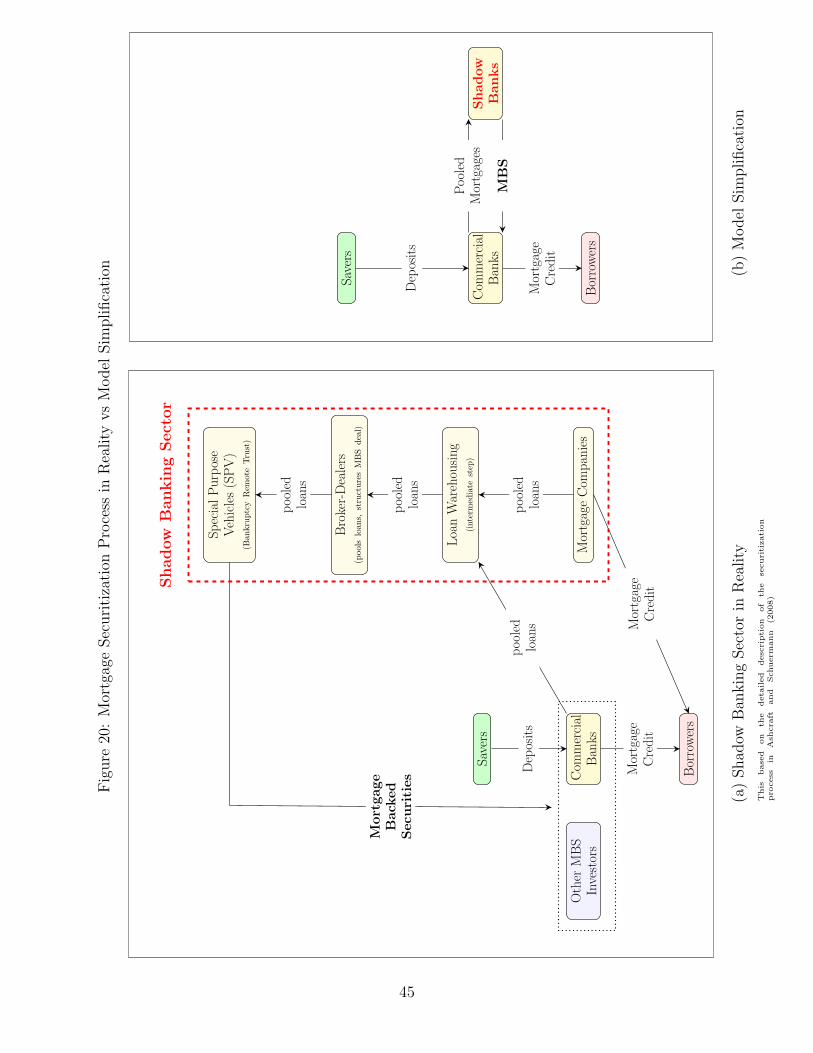
a two-layered mortgage securitizing financial sector comprised of mortgage issuing commer-
cial banks and mortgage securitizing shadow banks. Shadow banks in this context are the
Special Purpose Vehicles - the off-balance sheet entities owned by commercial or investment
3
banks who bought and packaged non-conforming5 mortgages into private mortgage backed
securities. This captures the institutional reality of this period, missed by standard mod-
els, that by providing an outlet for commercial banks to move their own lending off their
balance sheet shadow banks enabled commercial banks to loosen the regulatory constraints
that would limit a credit supply boom. Models that do not account for securitization as an
outlet for commercial banks will falsely reject the credit supply boom story.
The model captures the geographic dispersion of the US mortgage and housing markets
and idiosyncratic mortgage default risk by incorporating an island structure. There is a con-
tinuum of islands, and each island has a borrower, saver, and commercial bank. Households
can only interact with their island’s commercial bank. In each period a proportion of islands
receive a default shock which means borrowers on “hit” islands do not pay back a proportion
of debt. Commercial banks can choose to either hold the mortgages they issue or mortgage
backed securities. Shadow banks sit off-islands so can buy mortgages across islands and sell
to commercial banks an asset (the mortgage backed security) that pays the average mort-
gage return across islands. Because of the idiosyncratic risk involved in retaining individual
mortgages commercial banks hold mortgage backed securities as insurance. Without this id-
iosyncratic risk commercial banks would prefer to hold the mortgages they originate (earning
a greater return in expectation). Holding mortgage backed securities reassures savers that
the deposits issued by commercial banks will be paid back even on the default “hit” islands.
This allows commercial banks to intermediate more funds and expand total mortgage credit
provision on island - and thus overall mortgage credit supply.
The paper proceeds as follows. Section 2 presents the model. Section 3 presents the
calibration and simulation method. Section 4 explains the innovation in securitization mech-
anism. Section 5 presents and discusses the simulation results. And section 6 concludes.
5Those mortgages that fell outside the standards required for securitization by the Government SponsoredEnterprises (Fannie Mae & Freddie Mac).
4
2 The Model
2.1 Overview
I build a model in which idiosyncratic mortgage default risk micro-founds the existence
of mortgage backed securitization, and embed this model into a simplified version of the
housing in DSGE framework originated in Iacoviello and Neri (2010). The key innovation is
the addition of a two-layered mortgage securitizing financial sector comprised of mortgage
issuing commercial banks and mortgage securitizing shadow banks. Borrowers, savers, and
commercial banks exist in geographically disperse locations (islands). A commercial bank
can only take deposits from savers on their island and can only lend to borrowers on their
island. Each period a proportion of islands receive a default shock, on these “bad” islands
borrowers do not pay back a proportion (δ) of what they owe on their mortgage debt (RM,tbt).
Figure 2: The Model
Savers
Borrowers
Producers
FixedHousingSupply
Households
ShadowBanks
CommercialBanks
Deposits
MortgageCredit
Consumption Goods
LaborMBS
PooledMortgages
Housing
The model overlays an island structure onto a RBC model. Each island contains a bor-
rower household, a saver household, a commercial bank, and a producer who uses on island
labor to produce output that is 1-for-1 convertible into the consumption good. Households
can only interact with their local (on island) commercial bank.
Figure 3 illustrates the island structure of default. The commercial banking sector on
each island may only lend to households on their island. Every period a random fraction
ψ of islands are hit by a default shock, similar to Gertler and Kiyotaki (2010)’s island-
5
Figure 3: Risky Mortgage Lending
Full Repayment(RMtbt)
Full Repayment(RMtbt)
Partial Default((1− δ)RM,tbt)
1− ψ(Fraction of islands that are good)
ψ(Fraction of islands that are bad)
specific investment opportunity shock. On “bad” islands (those receiving a default shock)
the borrower only repays a fraction 1− δ of what they owe on their mortgage debt6. Where
RM,t is the mortgage rate and bt is the quantity of mortgage debt taken out by an individual
borrower.
The timing is as follows (see Figure 4): prior to the start of the period mortgages are
originated, commercial banks choose how to construct their balance sheet (between holding
their own mortgages and holding mortgage backed securities). And shadow banks choose
the quantity of pooled mortgages to buy and the quantity of mortgage backed securities to
issue. These decisions jointly determine the mortgage spread. At the start of a new period
the islands realize their default status. On a good island the borrower repays in full, on a
bad island the borrower defaults proportionally. Commercial banks across all islands repay
deposits, then commercial banks travel across islands to equalize credit conditions on islands
going into the next period7.
6This paper focuses on idiosyncratic risk, this framework could be extended to address aggregate mortgagemarket uncertainty by making ψ time-varying.
7Essentially there is a representative commercial banking sector but commercial banks across islandscannot insure each other until after deposits on island are repaid.
6
Figure 4: Default Timing
t t+ 1
Mort
gages O
rigina
ted
Mort
gages S
ecuritized
Default o
nBa
dIslands
Borro
wers:
repay
mortg
agesordefau
lt
All C
omme
rcialBanks:rep
aydeposits
Comm
ercial
Banks T
ravel
Repeats
...
Note on “Travel”: After deposits are repaid commercial banks move across islands to equalize credit condi-tions on all islands going into the next period. Essentially commercial banks are acting as a representativecommercial banking sector but they cannot insure each other against adverse island shocks until after de-posits are repaid.
Commercial banks can choose to retain the mortgages they issue on balance sheet (as
“portfolio loans”), or to sell them to the off-island securitizing shadow bank. The shadow
banking sector purchases mortgages from across all islands and packages them into “pass-
thru” mortgage backed securities (which payoff based on the aggregate mortgage market
return, averaged across islands). Shadow banks are able to divert funds, a la Gertler and
Kiyotaki (2010) and Meeks et al. (2017), and therefore are subject to an incentive compati-
bility constraint.
2.2 Households
There are two types of households. Savers are the ultimate source of funding for mortgage
debt. Borrowers are relatively impatient individuals who value housing and face a collateral
constraint when obtaining mortgage credit. Each household type risk shares in a large
family across islands an abstraction that focuses the idiosyncratic risk from island specific
default shocks entirely onto the financial sector in this model. Both household types have
log preferences in consumption, and borrowers have additively separable log preferences in
housing.
7
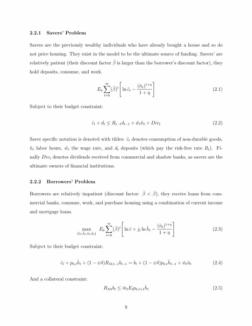
2.2.1 Savers’ Problem
Savers are the previously wealthy individuals who have already bought a house and so do
not price housing. They exist in the model to be the ultimate source of funding. Savers’ are
relatively patient (their discount factor β is larger than the borrower’s discount factor), they
hold deposits, consume, and work.
E0
∞∑t=0
(β)t
[ln ct −
(nt)1+η
1 + η
](2.1)
Subject to their budget constraint:
ct + dt ≤ Rt−1dt−1 + wtnt +Divt (2.2)
Saver specific notation is denoted with tildes: ct denotes consumption of non-durable goods,
nt labor hours, wt the wage rate, and dt deposits (which pay the risk-free rate Rt). Fi-
nally Divt denotes dividends received from commercial and shadow banks, as savers are the
ultimate owners of financial institutions.
2.2.2 Borrowers’ Problem
Borrowers are relatively impatient (discount factor: β < β), they receive loans from com-
mercial banks, consume, work, and purchase housing using a combination of current income
Where mt is the exogenous collateral value of housing, and ph,t is the price of housing.
Borrower specific notation is denoted with hats: ct denotes consumption of non-durable
goods, nt labor hours, wt the wage rate, and bt mortgage debt (RM,t is the mortgage rate).
jt is the borrower’s housing preference - shocks to jt are any factor unrelated to financing
conditions that move house prices.
Borrowers in this model risk share: the aggregate (across island) value of non-defaulted
housing and non-defaulted debt enters the borrower budget constraint (2.4). This means the
model abstracts from potentially interesting heterogeneity between borrowers with different
histories of default. This assumption is required for tractability outside of a heterogeneous
agent model of borrowers. However, this treatment still allows commercial banks to face
idiosyncratic risk from retaining their own lending, the focus of this paper.
Credit demand shocks are captured in two ways. One, via housing demand shocks (posi-
tive shocks to the housing preference parameter jt) which drive house prices up and therefore
push borrowers to demand larger mortgage balances to finance the purchase of more expen-
sive housing (via a collateral cycle effect this is possible). And two, housing collateral shocks
(positive shocks to the collateral value of housing mt) which directly expand the borrowers
ability to borrower via increasing the collateral value of their house.
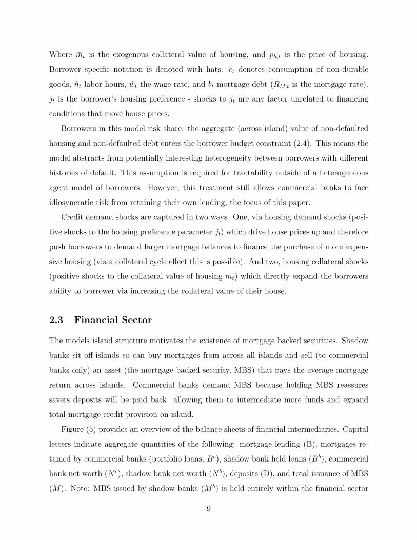
2.3 Financial Sector
The models island structure motivates the existence of mortgage backed securities. Shadow
banks sit off-islands so can buy mortgages from across all islands and sell (to commercial
banks only) an asset (the mortgage backed security, MBS) that pays the average mortgage
return across islands. Commercial banks demand MBS because holding MBS reassures
savers deposits will be paid back allowing them to intermediate more funds and expand
total mortgage credit provision on island.
Figure (5) provides an overview of the balance sheets of financial intermediaries. Capital
letters indicate aggregate quantities of the following: mortgage lending (B), mortgages re-
tained by commercial banks (portfolio loans, Bc), shadow bank held loans (Bb), commercial
bank net worth (N c), shadow bank net worth (N b), deposits (D), and total issuance of MBS
(M). Note: MBS issued by shadow banks (M b) is held entirely within the financial sector
9
Figure 5: Financial Sector Balance Sheet
Bb
Bc
Total MortgageCredit (B)
M
Bc
N c
D
Bb
N b
M
Mortgage Lending
assets
liabilitie
s
Commercial Banks
assets
liabilitie
s
Shadow Banks
Bb Pooled Loans Bc Portfolio Loans M Mortgage Backed Securities
D Deposits N c Commercial Bank Net Worth N b Shadow Bank Net Worth
Note: Portfolio Loans (Bc) are the loans originated and then retained by an individual commercial bank,these loans are subject to island specific default risk. In contrast the Pooled Loans (Bb) are the loanspurchased by shadow banks from across all islands, these loans are diversified so only have aggregate risknot island specific risk.
by commercial banks (M c), so that M =M c =M b.
2.3.1 Commercial Banking Sector
Commercial banks are constrained by the savers willingness to make deposits. Savers will
only make an additional deposit in their local commercial bank if they expect to be repaid
in full even in the event of being on a “bad” (default hit) island. This “solvency constraint”
requirement limits the ratio of portfolio mortgages to MBS the commercial bank can hold.
Commercial banks can can relax the solvency constraint via the securitization process selling
mortgages off their balance sheet and buying MBS which is diversified of their island specific
risk.
There exists a continuum of commercial banks indexed by c ∈[0, 1
]. Each period com-
mercial banks choose a specific island on which to locate for the purposes of mortgage lending
10
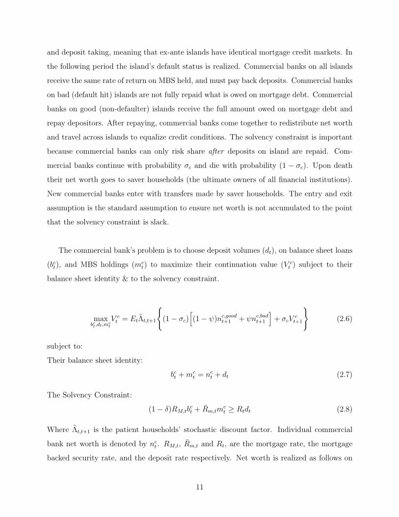
and deposit taking, meaning that ex-ante islands have identical mortgage credit markets. In
the following period the island’s default status is realized. Commercial banks on all islands
receive the same rate of return on MBS held, and must pay back deposits. Commercial banks
on bad (default hit) islands are not fully repaid what is owed on mortgage debt. Commercial
banks on good (non-defaulter) islands receive the full amount owed on mortgage debt and
repay depositors. After repaying, commercial banks come together to redistribute net worth
and travel across islands to equalize credit conditions. The solvency constraint is important
because commercial banks can only risk share after deposits on island are repaid. Com-
mercial banks continue with probability σc and die with probability (1 − σc). Upon death
their net worth goes to saver households (the ultimate owners of all financial institutions).
New commercial banks enter with transfers made by saver households. The entry and exit
assumption is the standard assumption to ensure net worth is not accumulated to the point
that the solvency constraint is slack.
The commercial bank’s problem is to choose deposit volumes (dt), on balance sheet loans
(bct), and MBS holdings (mct) to maximize their continuation value (V c
t ) subject to their
balance sheet identity & to the solvency constraint.
maxbct ,dt,m
ct
V ct = EtΛt,t+1
(1− σc)
[(1− ψ)nc,good
t+1 + ψnc,badt+1
]+ σcV
ct+1
(2.6)
subject to:
Their balance sheet identity:
bct +mct = nc
t + dt (2.7)
The Solvency Constraint:
(1− δ)RM,tbct + Rm,tm
ct ≥ Rtdt (2.8)
Where Λt,t+1 is the patient households’ stochastic discount factor. Individual commercial
bank net worth is denoted by nct . RM,t, Rm,t and Rt, are the mortgage rate, the mortgage
backed security rate, and the deposit rate respectively. Net worth is realized as follows on
11
good and bad islands.
nct+1 =
RM,tbct + Rm,tm
ct −Rtdt, if on a good island
(1− δ)RM,tbct + Rm,tm
ct −Rtdt, if on a bad island
(2.9)
The solvency constraint is the requirement that, when the banks island is hit with the default
shock, its revenue on mortgage lending and MBS holdings must exceed or be equal to its
obligation to depositors. Essentially the solvency constraint plays the role of a value-at-risk
(VaR) constraint8, where the probability of defaulting on deposits is 0.
Aggregate commercial banking sector net worth evolves according to:
N ct = (σc + ξc)
((1− δψ)RM,t−1B
ct−1 + Rm,t−1Mt−1
)− σcRt−1Dt−1 (2.10)
Where ξc is the proportional transfer saver households make to new entering commercial
banks.
2.3.2 Shadow Banking Sector
Shadow banks are constrained by the market’s willingness to hold their assets, the mortgage
backed security (MBS). This constraint is the Gertler and Kiyotaki (2010) running away
constraint. If this constraint exogenously loosens they are able to securitize more mortgage
credit, which allows commercial banks to provide more mortgage credit this is the innovation
in securitization credit supply shock.
Shadow Banks exist off-island. Each period they buy a perfectly diversified set of mort-
gages from every island and issue MBS which pay the average return on mortgage credit
across islands. They die with probability (1−σb) and survive with probability σb. They face
an agency problem that follows that in Meeks et al. (2017) and Gertler and Kiyotaki (2010).
The shadow bank’s problem is to purchased diversified (pooled) mortgage debt (bbt) and
issue MBS (mbt) to maximize their continuation value (V b
t ) subject to their balance sheet
identity and incentive compatibility constraint:
8Eg that in Adrian and Shin (2014).
12
maxbbt ,mb
tV bt = EtΛt,t+1
[(1− σb)n
bt+1 + σbV
bt+1
](2.11)
subject to:
Their balance sheet identity:
bbt = mbt + nb
t (2.12)
The incentive compatibility constraint:
V bt ≥ θb,tb
bt (2.13)
An individual shadow bank’s net worth evolves according to:
nbt+1 = (1− ψδ)RM,tb
bt︸ ︷︷ ︸
return on the diversified mortgage pool
− Rm,tmbt (2.14)
The shadow bank’s incentive compatibility constraint (2.13) captures the agency problem
between a shadow bank and the commercial banks that holds the MBS the shadow bank
issues. The literal interpretation of θb,t is as follows: each period the shadow bank is able
to choose to close down and take away a fraction θb,t of the amount repaid on the mortgage
debt the shadow bank owns. If the shadow bank chooses this they will never be trusted
again, they close down and forfeit their continuation value V bt . This constraint (2.13) limits
the quantity of MBS shadow banks can issue. Essentially θb,t indexes the trust that MBS
holders place in shadow banks. A fall in θb,t captures financial innovation of the sort expe-
rience prior to the financial crisis. Financial innovation in this context relates directly to
“credit enhancements”9- the implicit or explicit agreements such as tranching that were used
to reassure investors that MBS were nearly risk-free assets. An “innovation in securitiza-
tion” shock (exogenous drop in θb,t) captures in reduced form either: a) actual technological
improvements in credit enhancements, or b) an increase in investor’s perception about the
ability of credit enhancements to minimize MBS credit risk. With innovation in securiti-
zation shadow banks can hold mortgage credit in greater quantities with a lower spread,
9See Gorton and Souleles (2007) for a discussion of these Credit Enhancements.
13
meaning that the general equilibrium effect is lower mortgage spreads.
Aggregate shadow banking sector net worth evolves according to:
N bt = (σb + ξb)(1− δψ)RM,t−1B
bt−1 − σbRm,t−1Mt−1 (2.15)
Where ξb is the proportional transfer saver households make to new entering shadow banks.
2.4 Production
Production is based on labor and labor is differentiated across borrower and saver types.
This is a simplification of the Iacoviello and Neri (2010) framework.
Each island contains a goods producer who chooses saver (nt) and borrower (nt) labor to
maximize their profit (2.16) subject to their production function (2.17). Household members
can travel costlessly across islands to work and consume, so that wages and prices equalize
across islands (alternatively this can be considered as one aggregate producer), the producer
problem is:
maxnt,nt
Yt −[wtnt + wtnt
](2.16)
subject to:
Yt = Atnαt n
1−αt (2.17)
2.5 Market Clearing
Goods Market equilibrium
Yt − ph,t
[ht − (1− δψ)ht−1
]= ct + ct (2.18)
Total Housing:
H = ht (2.19)
Total lending:
Bt = Bct +Bb
t (2.20)
14
MBS market:
M ct =M b
t (2.21)
3 Calibration & Simulation
3.1 Calibration
Table 1: Calibrated Parameters
Parameter Value Description
Macroeconomic Parameters
β 0.9943 Saver’s discount factor
β 0.97 Borrower’s discount factorA 1 Steady state level of TFPα 0.64 Labor income share of saversη 1 Inverse of the Frisch elasticity of labor supplyHousing and Financial ParametersH 1 Total inelastic supply of housingσc, σb 0.95 Financial institution survival probabilitym 0.92 Housing collateral valuej 0.067 Borrower housing preference parameterψ 1.3% Quarterly mortgage delinquency rateδ 23.8% On island defaultθb 0.60 Fraction of pooled loans that are divertibleξc 0.0028 Fraction of assets transfered to new commercial banksξb 0.0042 Fraction of assets transfered to new shadow banks
3.1.1 Macroeconomic Parameters:
This set of parameters either match well established calibrations in the literature, or target
an average of the 1990s data. β is set to target the average real Fed Funds rate in the
1990s data (of 2.28% annualized10). β is set to match the calibration in Iacoviello and Neri
10The average nominal Fed Funds rate (FEDFUNDS) in this period is 5.14% and the average growth inthe Consumer Price Index (CPIAUSCSL) is 2.86%
15
(2010). The relative impatience has a minimal effect on the co-movement of house prices
and mortgage credit but does not effect the overall results appreciably. The level of TFP in
steady state is normalized to 1. The calibration of the labor income share going to savers
(α) comes from Justiniano et al. (2015) who identify borrowers as households whose liquid
assets are less than two months of their total income - using the 1992, 1995 and 1998 Survey
of Consumer Finances (SCF). Following Justiniano et al. (2015) the Frisch elasticity of labor
supply(
1η
)is set to 1.
3.1.2 Housing and Financial Parameters:
The supply of housing H is normalized to 1. σc and σb target an expected survival horizon
for commercial and shadow banks of 5 years, consistent with the literature (eg Gertler and
Kiyotaki, 2015). The collateral value of housing (m) and the borrower’s housing prefer-
ence parameter (j) jointly target a mortgage debt to borrower income ratio of 0.811, and a
calculated loan-to-value (LTV) ratio of 90%12.
3.1.3 Simulation Initialization Targets:
The remaining parameters: δ, θb, ξc, ξb, and ψ which pertain most directly to the financial
sector, jointly target the moments in the 2000 Q1 - 2000 Q4 data in table 2. This narrower
target period better reflects the condition of the private securitization market, because the
early 1990s were characterized by only a handful of private securitization deals. The first
four parameters target the spread and balance sheet moments in table 2 and then ψ is set so
that the product of ψ (the fraction of islands that are bad islands) and δ (the proportional
default on bad islands) jointly target the fraction of mortgage dollars entering serious (90+
day) delinquency in the Quarterly Report on Household Debt and Credit (0.3180%).
The data series on the mortgage spread is the spread of the average mortgage rate in
the PLSD over the 10 year US Treasury yield, using the adjusted for borrower quality series
in Justiniano et al. (2017). The commercial bank asset composition is that of depository
11This follows the target in Justiniano et al. (2019): they identify borrowers as households whose liquidassets are less than two months of their total income - using the 1992, 1995 and 1998 SCF.
12This is a compromise between the higher documented LTV ratios in the non-conforming mortgage pool,and maintaining consistency with similar targets eg Justiniano et al. (2015) in the literature.
16
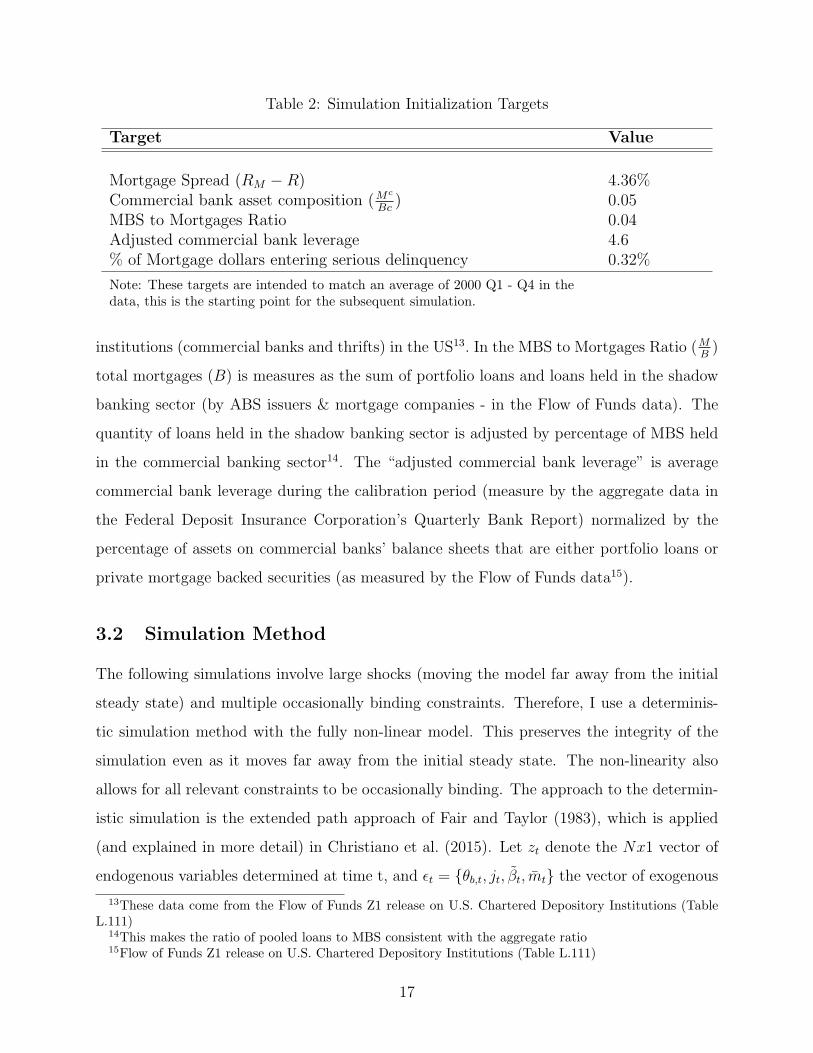
Table 2: Simulation Initialization Targets
Target Value
Mortgage Spread (RM −R) 4.36%Commercial bank asset composition (M
c
Bc) 0.05
MBS to Mortgages Ratio 0.04Adjusted commercial bank leverage 4.6% of Mortgage dollars entering serious delinquency 0.32%
Note: These targets are intended to match an average of 2000 Q1 - Q4 in thedata, this is the starting point for the subsequent simulation.
institutions (commercial banks and thrifts) in the US13. In the MBS to Mortgages Ratio (MB)
total mortgages (B) is measures as the sum of portfolio loans and loans held in the shadow
banking sector (by ABS issuers & mortgage companies - in the Flow of Funds data). The
quantity of loans held in the shadow banking sector is adjusted by percentage of MBS held
in the commercial banking sector14. The “adjusted commercial bank leverage” is average
commercial bank leverage during the calibration period (measure by the aggregate data in
the Federal Deposit Insurance Corporation’s Quarterly Bank Report) normalized by the
percentage of assets on commercial banks’ balance sheets that are either portfolio loans or
private mortgage backed securities (as measured by the Flow of Funds data15).
3.2 Simulation Method
The following simulations involve large shocks (moving the model far away from the initial
steady state) and multiple occasionally binding constraints. Therefore, I use a determinis-
tic simulation method with the fully non-linear model. This preserves the integrity of the
simulation even as it moves far away from the initial steady state. The non-linearity also
allows for all relevant constraints to be occasionally binding. The approach to the determin-
istic simulation is the extended path approach of Fair and Taylor (1983), which is applied
(and explained in more detail) in Christiano et al. (2015). Let zt denote the Nx1 vector of
endogenous variables determined at time t, and ϵt = θb,t, jt, βt, mt the vector of exogenous
13These data come from the Flow of Funds Z1 release on U.S. Chartered Depository Institutions (TableL.111)
14This makes the ratio of pooled loans to MBS consistent with the aggregate ratio15Flow of Funds Z1 release on U.S. Chartered Depository Institutions (Table L.111)
17
deterministic variables realized at time t. Each period the agents realize an unexpected
shock (to either θb,t, jt, βt or mt) and expect the economy to transition to a new steady state
consistent with the realization of that shock. In t=1 the starting point of the deterministic
simulation is the initial steady state, in t ≥ 2 the starting point is the vector of endogenous
variables in t− 1.
4 The Innovation in Securitization Channel
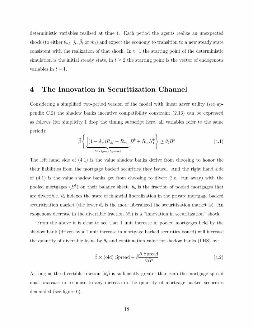
Considering a simplified two-period version of the model with linear saver utility (see ap-
pendix C.2) the shadow banks incentive compatibility constraint (2.13) can be expressed
as follows (for simplicity I drop the timing subscript here, all variables refer to the same
period):
β
[(1− δψ)RM − Rm
]︸ ︷︷ ︸
Mortgage Spread
Bb + RmNb1
≥ θbB
b (4.1)
The left hand side of (4.1) is the value shadow banks derive from choosing to honor the
their liabilities from the mortgage backed securities they issued. And the right hand side
of (4.1) is the value shadow banks get from choosing to divert (i.e. run away) with the
pooled mortgages (Bb) on their balance sheet. θb is the fraction of pooled mortgages that
are divertible. θb indexes the state of financial liberalization in the private mortgage backed
securitization market (the lower θb is the more liberalized the securitization market is). An
exogenous decrease in the divertible fraction (θb) is a “innovation in securitization” shock.
From the above it is clear to see that 1 unit increase in pooled mortgages held by the
shadow bank (driven by a 1 unit increase in mortgage backed securities issued) will increase
the quantity of divertible loans by θb and continuation value for shadow banks (LHS) by:
β × (old) Spread + β∂ Spread
∂Bb(4.2)
As long as the divertible fraction (θb) is sufficiently greater than zero the mortgage spread
must increase in response to any increase in the quantity of mortgage backed securities
demanded (see figure 6).
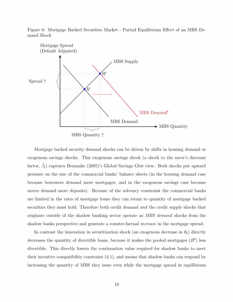
18
Figure 6: Mortgage Backed Securities Market - Partial Equilibrium Effect of an MBS De-mand Shock
MBS Quantity
Mortgage Spread(Default Adjusted)
MBS Supply
MBS Demand
MBS Demand′
H
H ′
MBS Quantity ↑
Spread ↑
Mortgage backed security demand shocks can be driven by shifts in housing demand or
exogenous savings shocks. This exogenous savings shock (a shock to the saver’s discount
factor, βt) captures Bernanke (2005)’s Global Savings Glut view. Both shocks put upward
pressure on the size of the commercial banks’ balance sheets (in the housing demand case
because borrowers demand more mortgages, and in the exogenous savings case because
savers demand more deposits). Because of the solvency constraint the commercial banks
are limited in the ratio of mortgage loans they can retain to quantity of mortgage backed
securities they must hold. Therefore both credit demand and the credit supply shocks that
originate outside of the shadow banking sector operate as MBS demand shocks from the
shadow banks perspective and generate a counter-factual increase in the mortgage spread.
In contrast the innovation in securitization shock (an exogenous decrease in θb) directly
decreases the quantity of divertible loans, because it makes the pooled mortgages (Bb) less
divertible. This directly lowers the continuation value required for shadow banks to meet
their incentive compatibility constraint (4.1), and means that shadow banks can respond by
increasing the quantity of MBS they issue even while the mortgage spread in equilibrium
19
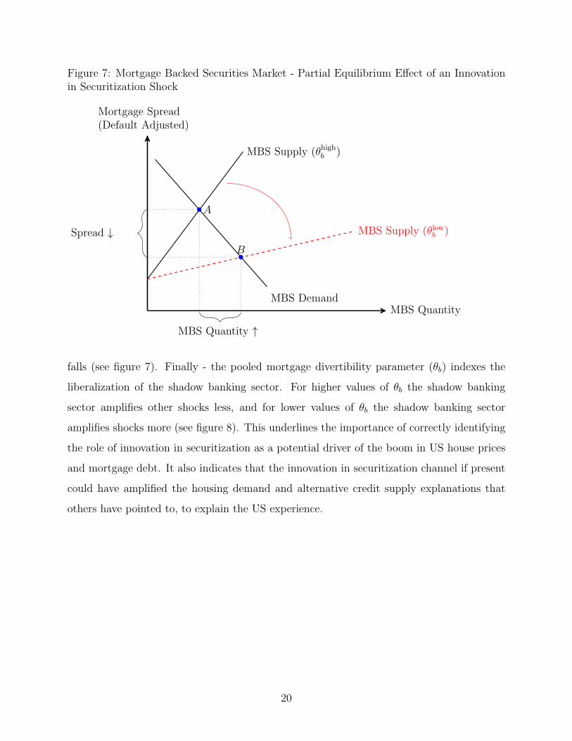
Figure 7: Mortgage Backed Securities Market - Partial Equilibrium Effect of an Innovationin Securitization Shock
MBS Quantity
Mortgage Spread(Default Adjusted)
MBS Supply (θhighb )
MBS Supply (θlowb )
MBS Demand
A
B
MBS Quantity ↑
Spread ↓
falls (see figure 7). Finally - the pooled mortgage divertibility parameter (θb) indexes the
liberalization of the shadow banking sector. For higher values of θb the shadow banking
sector amplifies other shocks less, and for lower values of θb the shadow banking sector
amplifies shocks more (see figure 8). This underlines the importance of correctly identifying
the role of innovation in securitization as a potential driver of the boom in US house prices
and mortgage debt. It also indicates that the innovation in securitization channel if present
could have amplified the housing demand and alternative credit supply explanations that
others have pointed to, to explain the US experience.
20
Figure 8: Mortgage Backed Securities Market - A More Liberalized Shadow Banking SectorMagnifies Other Shocks
MBS Quantity
Mortgage Spread(Default Adjusted)
MBS Supply (θhighb )
MBS Supply (θlowb )
MBS Demand
MBS Demand′
H
L
H ′
L′
∆MBS (θhighb ) ∆MBS (θlowb )
∆ Spread (θhighb )
∆ Spread (θlowb )
Figures 9, 10, and 11 make the qualitative amplification point in figure 8 quantitatively.
In each figure respectively I calibrate a 1-off permanent shock to housing preference, housing
collateral, and saver patience to generate a 1% increase in total outstanding mortgage credit
in the pre-boom (year 2000) version of the model. I then run the same shock at the Securiti-
zation Peak, Housing Demand Peak, and Exogenous Savings Peak (that is the model version
consistent with the various 2006 Q4 versions of the model in the following horse-race). The
qualitative point in figure 8 - for all three 1-off shocks the Securitization Peak amplifies the
impact of the shock on house prices and mortgage credit the most relative to the other peaks.
And in all three cases the response of the mortgage spread is least under the Securitization
Note the housing demand shock is an exogenous increase in the borrowers’ preference for housing parameter(jt), in their utility function - equation (2.3). The mortgage spread is plotted in basis points deviation fromsteady state.
Figure 10: Transmission of a Housing Collateral Shock
Note: The housing collateral shock is an exogenous increase in mt, the housing collateral value in theborrowers’ collateral constraint - equation (2.5).
22
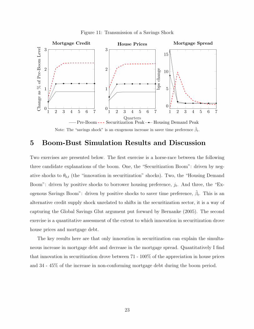
Figure 11: Transmission of a Savings Shock
1 2 3 4 5 6 70
1
2
3
Chan
geas
%of
Pre-B
oom
Level
Mortgage Credit
Pre-Boom Securitization Peak Housing Demand Peak
1 2 3 4 5 6 70
1
2
3
Quarters
House Prices
1 2 3 4 5 6 70
5
10
15
bpschan
ge
Mortgage Spread
Note: The “savings shock” is an exogenous increase in saver time preference βt.
5 Boom-Bust Simulation Results and Discussion
Two exercises are presented below. The first exercise is a horse-race between the following
three candidate explanations of the boom. One, the “Securitization Boom”: driven by neg-
ative shocks to θb,t (the “innovation in securitization” shocks). Two, the “Housing Demand
Boom”: driven by positive shocks to borrower housing preference, jt. And three, the “Ex-
ogenous Savings Boom”: driven by positive shocks to saver time preference, βt. This is an
alternative credit supply shock unrelated to shifts in the securitization sector, it is a way of
capturing the Global Savings Glut argument put forward by Bernanke (2005). The second
exercise is a quantitative assessment of the extent to which innovation in securitization drove
house prices and mortgage debt.
The key results here are that only innovation in securitization can explain the simulta-
neous increase in mortgage debt and decrease in the mortgage spread. Quantitatively I find
that innovation in securitization drove between 71 - 100% of the appreciation in house prices
and 34 - 45% of the increase in non-conforming mortgage debt during the boom period.
23
5.1 Horse-Race to Match House Price Growth
In each of the three competing simulations the individual shock series is calibrated to target
the peak in house prices during the boom (47% in 2006 Q4 according to the Case-Shiller Real
House Price Index). Figure 12 shows the target series and corresponding shock processes for
each simulation in the horse-race. The goal here is to match the boom in house prices, and
then ask how much of the bust can be matched by reversing the shock that drove the boom.
Figure 12: Matching Real House Price Growth
2000Q4 2006Q4 2012Q1
100
110
120
130
140
150
Index,20
00Q4=
100
Securitization Boom
2000Q4 2006Q4 2012Q1
100
110
120
130
140
150
Housing Demand Boom
Model Data
2000Q4 2006Q4 2012Q1
100
110
120
130
140
150
Exogenous Savings BoomReal House Prices, Data vs Model
2000Q4 2006Q4 2012Q10
0.2
0.4
0.6
Shock
Level
Securitization Shocks, θb,t
2000Q4 2006Q4 2012Q1
0.067
0.10
Housing Demand, jt
2000Q4 2006Q4 2012Q1
0.9943
1
Exogenous Savings, βShock Series
In this figure each column is a different simulation in the horse-race. The green shaded area indicates thehousing collateral constraint is slack, the red shaded area indicates the housing collateral constraint binds.The vertical blue line is 2006Q4 (the peak period for real house prices according to the Case-Shiller Index).
24
Figure 13: Only the Securitization Boom Explains Mortgage Spreads
2000Q4 2006Q4 2012Q1
2
4
6
AnnualPercentagePoints
Securitization Boom
2000Q4 2006Q4 2012Q1
2
4
6
Housing Demand Boom
Model Data
2000Q4 2006Q4 2012Q1
2
4
6
Exogenous Savings BoomModel vs Data: Mortgage Rate Spread over Risk-Free Rate
In this figure each column is a different simulation in the horse-race. The green shaded area indicates thehousing collateral constraint is slack, the red shaded area indicates the housing collateral constraint binds.The vertical blue line is 2006Q4 (the peak period for real house prices according to the Case-Shiller Index).
The key result, captured in figure 13 in this simulation is that only the innovation in
securitization shocks can match (the direction & magnitude) of the spread between the
mortgage rate and the risk free rate. Unsurprisingly the housing demand driven boom (a
demand for credit shock) puts upward pressure on the mortgage spread. More interestingly
the exogenous savings expansion, which operates like the inelastic credit supply shock in
Justiniano et al. (2019) and in this closed economy model stand in for an influx of foreign
credit, also generates upward pressure on the mortgage spread. This is because the exogenous
increase in savings drives deposits up, expanding the commercial banking sector’s aggregate
balance sheet. To expand their balance sheets commercial banks must hold more MBS to
continue to meet the solvency constraint - this increases the demand shadow banks face for
MBS, and because of the incentive compatibility constraint faced by shadow banks to increase
quantity of MBS they issue they require an increased spread. This result underlines the
necessity of modeling the securitization process, while the generalized credit supply expansion
– “exogenous savings boom” – is a credit supply shock, the counter-factual implications
suggest that it is likely not the credit supply shock that drove the US housing and mortgage
market during the 2000s.
25
Additionally the Securitization boom generates the most volatility in borrower and saver
consumption (figure 14) and is the only channel which generates a quantitatively reasonable
response of several moments in the private securitization market (see Figure 18 in Appendix
B). Lastly the three candidate booms are indistinguishable in the response of mortgage debt
and the borrower debt-to-annual income ratio (see Figure 17 in Appendix B).
Figure 14: Consumption is Most Volatile Under in the Securitization Boom
2000Q4 2006Q4 2012Q195
100
105
110
Index,20
00Q4=
100
Securitization Boom
2000Q4 2006Q4 2012Q195
100
105
110
Housing Demand Boom
Borrower Saver
2000Q4 2006Q4 2012Q195
100
105
110
Exogenous Savings BoomConsumption: Borrower vs Saver
The green shaded area indicates the housing collateral constraint is slack, the red shaded area indicates thehousing collateral constraint binds. The vertical blue line is 2006Q4 (the peak period for real house pricesaccording to the Case-Shiller Index).
5.2 Measuring the Contribution of Innovation in Securitization
In this section I put upper and lower bounds on the model’s prediction as to the extent to
which innovation in securitization could have driven house price growth. The data series
most closely related to the innovation in securitization shocks are: private mortgage backed
security issuance and the securitization rate. Issuance is the flow of private mortgage backed
securities produced by the shadow banking sector each quarter. This grew by over 790%
between 2000 Q4 and its peak in 2005 Q3 (See the leftmost subplot in Figure 15), matching
this data series gives a lower bound as to the magnitude of the innovation in securitization
channel (see sold black line in Figure 15). In contrast matching the securitization rate gives
an upper bound as to the magnitude of the innovation in securitization channel (see dotted
26
black line in Figure 15). The securitization rate is the ratio of private mortgage backed
security issuance to non-conforming mortgages originated in any given quarter. It is another
flow series that is closely related to the constraints faced by the shadow banking sector when
issuing private mortgage backed securities.
Figure 15: Matching Moments - Upper and Lower Bounds
2000Q4 2006Q4 2012Q10
200
400
600
800
1,000
1,200
Index,20
00Q4=
100
MBS Issuance
2000Q4 2006Q4 2012Q10
10
20
30percentage
pointchan
ge
Securitization Rate
Data Targeting MBS Issuance (Lower Bound) Targeting the Securitization Rate (Upper Bound)
2000Q4 2006Q4 2012Q10
0.2
0.4
0.6
level
Securitization Shocks, θb,t
Here the upper estimate of the securitization shock series (targeted to match the securitization rate - theratio of MBS issued to mortgage debt originated) is the dot-dashed black line. The lower estimate of thesecuritization shock series is the solid black line (targeted to match the growth in private mortgage backedsecurity issuance). The dashed red line is the data.
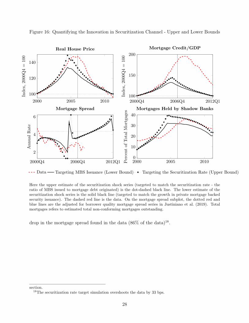
Figure 16 shows the upper and lower bounds the securitization rate target simulation and
the MBS issuance target simulation put on the extent to which innovation in securitization
drove the boom in house prices, mortgage credit, the mortgage spread, and the percentage
of the stock of (non-conforming) mortgages held by the shadow banking sector. The results
of the two simulations suggest that the innovation in securitization can explain between
72% and over 100% of the increase in real house prices seen in the data16. innovation in
securitization drives between 34.3% to 45.8% of the increase in mortgage credit relative to
GDP17. innovation in securitization explains at least 235 basis points of the 273 basis point
16The securitization rate target simulation overshoots the real house price peak by 3%.17The multiplier between house price growth and mortgage credit growth does not match the data. This
could be in part because the model’s supply of housing is fixed, adding housing investment may bring themultiplier more in line with the data. This would not change the qualitative point made in the proceeding
27
Figure 16: Quantifying the Innovation in Securitization Channel - Upper and Lower Bounds
2000 2005 2010
100
120
140
Index,20
00Q4=
100
Real House Price
2000Q4 2006Q4 2012Q1100
150
200
Index,20
00Q4=
100
Mortgage Credit/GDP
2000Q4 2006Q4 2012Q1
2
4
6
Annual
Rate
Mortgage Spread
Data Targeting MBS Issuance (Lower Bound) Targeting the Securitization Rate (Upper Bound)
2000 2005 20100
10
20
30
40
Percentof
Total
Mortgag
es
Mortgages Held by Shadow Banks
Here the upper estimate of the securitization shock series (targeted to match the securitization rate - theratio of MBS issued to mortgage debt originated) is the dot-dashed black line. The lower estimate of thesecuritization shock series is the solid black line (targeted to match the growth in private mortgage backedsecurity issuance). The dashed red line is the data. On the mortgage spread subplot, the dotted red andblue lines are the adjusted for borrower quality mortgage spread series in Justiniano et al. (2019). Totalmortgages refers to estimated total non-conforming mortgages outstanding.
drop in the mortgage spread found in the data (86% of the data)18.
section.18The securitization rate target simulation overshoots the data by 33 bps.
28
6 Conclusion
In this paper I build a model in which the interaction of regulated commercial banks and
the unregulated shadow banking sector is crucial. In the model the existence of mortgage
backed securitization is based on idiosyncratic mortgage default risk. Shadow banks face
a financial constraint on their balance sheet which relaxes over the boom period (2000 -
2006). This is “Innovation in Securitization”. This innovation captures a number of factors
including: the increased sophistication and use of tranching during this period, and increased
market familiarity with private mortgage backed securitization (relative to the much older
government associated securitization19). I find that this innovation was a primary driver
of the increase in house prices and mortgage debt in the US between 2000 and 2006. The
Innovation in Securitization shocks account for 71 - 100% of the increase in house prices and
34 - 45% of the increase in non-conforming mortgage debt observed in the data.
Additionally I show that other candidate explanations (a housing demand driven boom
or a savings driven boom – the Global Savings Glut view) cannot on their own match the
mortgage spread dynamics. For the housing demand driven boom the balance sheet effect
amplifies the upward pressure on the mortgage spread. For the exogenous savings boom
the balance sheet effect quantitatively reverses the initial negative impact on the mortgage
spread. Because of the feedback driven by the balance sheet effect, capturing it shows that
these two alternative explanations of the 2000 - 2006 US boom generate counter-factual
implications for the mortgage spread. This is not to say that the model rules out housing
demand and exogenous savings shocks as amplifiers of the securitization driven boom. I
find that in a more liberalized20 shadow banking sector the impact of housing demand and
savings shocks on mortgage credit growth and house price growth are amplified relative to the
pre-boom version of the model, and the response of the mortgage spread is moderated. The
amplification effect is particularly strong for the transmission of savings shocks - suggesting
securitization played an important role in amplifying the impact of inflows of foreign savings
into the U.S. during this period.
In ongoing work I am exploring the impact of macro-prudential regulation of commercial
19Mortgage backed securitization done by Fannie Mae, Freddie Mac, and Ginnie Mae.20The model after a series of positive innovation in securitization shocks.
29
banks in this model, particularly the potential leakages and interactions with the shadow
banking sector.
30
References
Adrian, Tobias and Hyun Song Shin, “Procyclical leverage and value-at-risk,” Review
of Financial Studies, 2014, 27 (2), 373–403. [Cited on page 12.]
Ashcraft, Adam B and Til Schuermann, “Federal Reserve Bank of New York Staff
Reports Understanding the Securitization of Subprime Mortgage Credit,” New York, 2008,
2 (318), 1779–1808. [Cited on page 45.]
Bernanke, Ben S., “The global saving glut and the U.S. current account deficit,” Technical
Report 2005. [Cited on pages 19 and 23.]
Christiano, Lawrence J., Martin S. Eichenbaum, and Mathias Trabandt, “Under-
standing the Great Recession,” American Economic Journal: Macroeconomics, January
2015, 7 (1), 110–167. [Cited on page 17.]
Fair, Ray C and John B Taylor, “Solution and Maximum Likelihood Estimation of
Dynamic Nonlinear Rational Expectations Models,” Econometrica, July 1983, 51 (4),
1169–1185. [Cited on page 17.]
Gertler, Mark and Nobuhiro Kiyotaki, Financial intermediation and credit policy in
business cycle analysis, Vol. 3, Elsevier Ltd, 2010. [Cited on pages 5, 7, and 12.]
and , “Banking, Liquidity, and Bank Runs in an Infinite Horizon Economy,” American
Economic Review, July 2015, 105 (7), 2011–2043. [Cited on page 16.]
Gorton, Gary B. and Nicholas S. Souleles, “Special Purpose Vehicles and Securiti-
zation,” in “The Risks of Financial Institutions” NBER Chapters, National Bureau of
Economic Research, Inc, May 2007, pp. 549–602. [Cited on page 13.]
Iacoviello, Matteo and Stefano Neri, “Housing Market Spillovers: Evidence from an
Estimated DSGE Model,” American Economic Journal: Macroeconomics, April 2010, 2
(2), 125–164. [Cited on pages 3, 5, 14, and 15.]
Justiniano, Alejandro, Giorgio E. Primiceri, and Andrea Tambalotti, “Household
leveraging and deleveraging,” Review of Economic Dynamics, January 2015, 18 (1), 3–20.
[Cited on page 16.]
, , and , “The Mortgage Rate Conundrum,” Working Paper Series WP-2017-23,
Federal Reserve Bank of Chicago August 2017. [Cited on page 16.]
31
, , and , “Credit Supply and the Housing Boom,” Journal of Political Economy,
2019, 127 (3), 1317–1350. [Cited on pages 2, 16, 25, and 28.]
Kaplan, Greg, Kurt Mitman, and Giovanni L. Violante, “The Housing Boom and
Bust: Model Meets Evidence,” NBER Working Papers 23694, National Bureau of Eco-
nomic Research, Inc August 2017. [Cited on page 2.]
Meeks, Roland, Benjamin Nelson, and Piergiorgio Alessandri, “Shadow Banks and
Macroeconomic Instability,” Journal of Money, Credit and Banking, 2017, 49 (7), 1483–
1516. [Cited on pages 7 and 12.]
Mian, Atif and Amir Sufi, Household Debt and Defaults from 2000 to 2010: The Credit
Supply View, Cambridge University Press, [Cited on page 2.]
Pozsar, Zoltan, Tobias Adrian, Adam B. Ashcraft, and Hayley Boesky, “Shadow
Banking,” Technical Report 458, Federal Reserve Bank of New York Staff Reports 2012.
[Cited on page 44.]
Shiller, Robert J., “Understanding recent trends in house prices and homeownership,”
Proceedings - Economic Policy Symposium - Jackson Hole, 2007, pp. 89–123. [Cited on
Incentive compatibility constraint (binding if λbt ≥ 0):
ϕbt ≤
vbmt
θb,t − µbM,t
(A.22)
Marginal Value of Loans (Note: µbM,t := vbMt − vbmt):
µbM,t = EtΛt,t+1Ω
bt+1
[(1− ψδ)RMt − Rm,t
](A.23)
Marginal Value of MBS:
vbmt = EtΛt,t+1Ωbt+1Rmt (A.24)
Balance Sheet Identity:
Bbt = N b
t +M bt (A.25)
Aggregate Shadow Bank Net Worth:
N bt = (σb + ξb)(1− ψδ)RM,t−1B
bt−1 − σbRm,t−1M
bt−1 (A.26)
Shadow Bank leverage:
ϕbt =
Bbt
N bt
(A.27)
Market Clearing:
H = ht (A.28)
ct + ct = Yt − ph,t
[ht − (1− δψt)ht−1
](A.29)
M ct =M b
t (A.30)
Bt = Bct +Bb
t (A.31)
35
B Boom-Bust Simulation Additional Results
Figure 17: Candidate Booms are Indistinguishable on Credit Growth and Change in Bor-rower Indebtedness
2000Q4 2006Q4 2012Q1
100
120
140
160
180
200
Index,200
0Q4=
100
Securitization Boom
2000 2005 2010
100
120
140
160
180
200
Housing Demand Boom
Model Data
2000Q4 2006Q4 2012Q1
100
120
140
160
180
200
Exogenous Savings BoomMortgage Credit to GDP Index
2000Q4 2006Q4 2012Q1
8
12
16
Ratio
Securitization Boom
2000Q4 2006Q4 2012Q1
8
12
16
Housing Demand Boom
2000Q4 2006Q4 2012Q1
8
12
16
Exogenous Savings BoomMortgage Debt to Borrower Annual Income
The green shaded area indicates the housing collateral constraint is slack, the red shaded area indicates thehousing collateral constraint binds. The vertical blue line is 2006Q4 (the peak period for real house pricesaccording to the Case-Shiller Index).
36
Figure 18: Horse-Race: Only the Securitization Boom can Match Secondary Market Mo-ments
2000Q4 2006Q4 2012Q10
10
20
30
percentage
pointchange
Securitization Boom
2000Q4 2006Q4 2012Q10
10
20
30
Housing Demand Boom
2000Q4 2006Q4 2012Q10
10
20
30
Exogenous Savings BoomModel vs Data: Securitization Rate
2000Q4 2006Q4 2012Q10
10
20
30
%pointchan
ge
Securitization Boom
2000Q4 2006Q4 2012Q10
10
20
Housing Demand Boom
2000Q4 2006Q4 2012Q10
10
20
Exogenous Savings BoomModel vs Data: % of Mortgages in Shadow Banking Sector
2000Q4 2006Q4 2012Q10
500
1,000
Index,200
0Q4=
100
Securitization Boom
2000Q4 2006Q4 2012Q10
500
1,000
Housing Demand Boom
Model Data
2000Q4 2006Q4 2012Q10
500
1,000
Exogenous Savings BoomModel vs Data: MBS Issuance
The green shaded area indicates the housing collateral constraint is slack, the red shaded area indicates thehousing collateral constraint binds. The vertical blue line is 2006Q4 (the peak period for real house pricesaccording to the Case-Shiller Index). The securitization rate is the ratio of mortgage backed securities issuedto mortgage debt originated in a given quarter, it is a flow measure of the extent to which mortgages werebeing originated and then quickly sold. 37
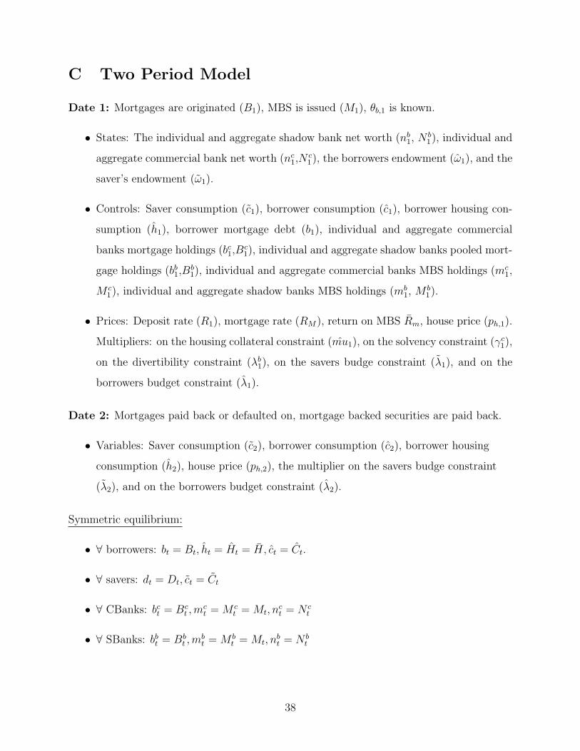
C Two Period Model
Date 1: Mortgages are originated (B1), MBS is issued (M1), θb,1 is known.
• States: The individual and aggregate shadow bank net worth (nb1, N